1

Statistical Inference

Dr fahd amjad

2

Why study statistics

“without data, you are just another person with an opinion.”

Statistics is the scientific discipline that provides us methods to make sense of data

Fields – Medicine, agriculture, engineering, social sciences etc.

3

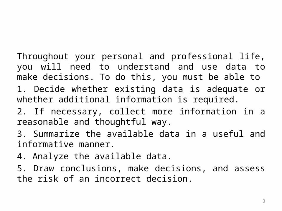
Throughout your personal and professional life, you will need to understand and use data to make decisions. To do this, you must be able to1. Decide whether existing data is adequate or whether additional information is required.2. If necessary, collect more information in a reasonable and thoughtful way.3. Summarize the available data in a useful and informative manner.4. Analyze the available data.5. Draw conclusions, make decisions, and assess the risk of an incorrect decision.

4

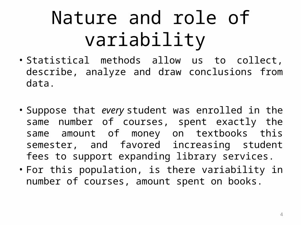
Nature and role of variability

• Statistical methods allow us to collect, describe, analyze and draw conclusions from data.

• Suppose that every student was enrolled in the same number of courses, spent exactly the same amount of money on textbooks this semester, and favored increasing student fees to support expanding library services.

• For this population, is there variability in number of courses, amount spent on books.

5

• The situation just described is obviously unrealistic. Populations with no variability are exceedingly rare, and they are of little statistical interest because they present no challenge! In fact, variability is almost universal.

• It is variability that makes life (and the life of a statistician, in particular) interesting. We need to understand variability to be able to collect, describe, analyze, and draw conclusions from data in a sensible way.

6

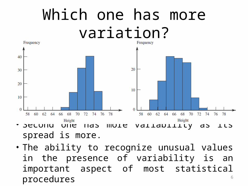
Which one has more variation?

• Second one has more variability as its spread is more.

• The ability to recognize unusual values in the presence of variability is an important aspect of most statistical procedures

7

Statistics and data analysis process

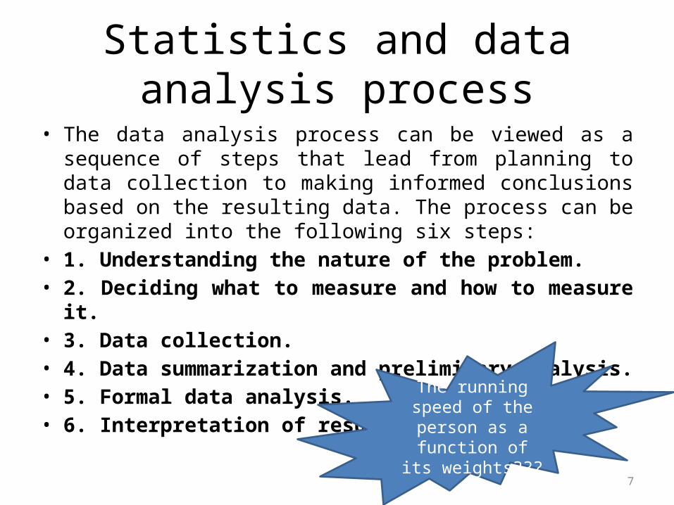
• The data analysis process can be viewed as a sequence of steps that lead from planning to data collection to making informed conclusions based on the resulting data. The process can be organized into the following six steps:

• 1. Understanding the nature of the problem.• 2. Deciding what to measure and how to measure it.• 3. Data collection.• 4. Data summarization and preliminary analysis.• 5. Formal data analysis.• 6. Interpretation of results. The running speed of

the person as a function of its

weights???

8

Sample and population

• The entire collection of individuals or objects about which information is desired is called the population of interest.

• A sample is a subset of the population, selected for study

9

Types of data

• The individuals or objects in any particular population typically possess many characteristics that might be studied.

• A variable is any characteristic whose value may change from one individual or object to another. For example, calculator brand is a variable, and so are number of textbooks purchased and distance to the university.

• Data result from making observations either on a single variable or simultaneously on two or more variables.

10

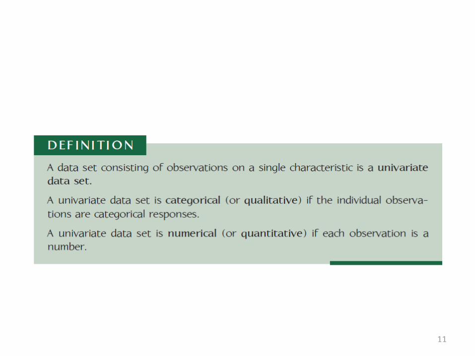
• A univariate data set consists of observations on a single variable made on individuals in a sample or population.

• There are two types of univariate data sets: categorical and numerical.

11

12

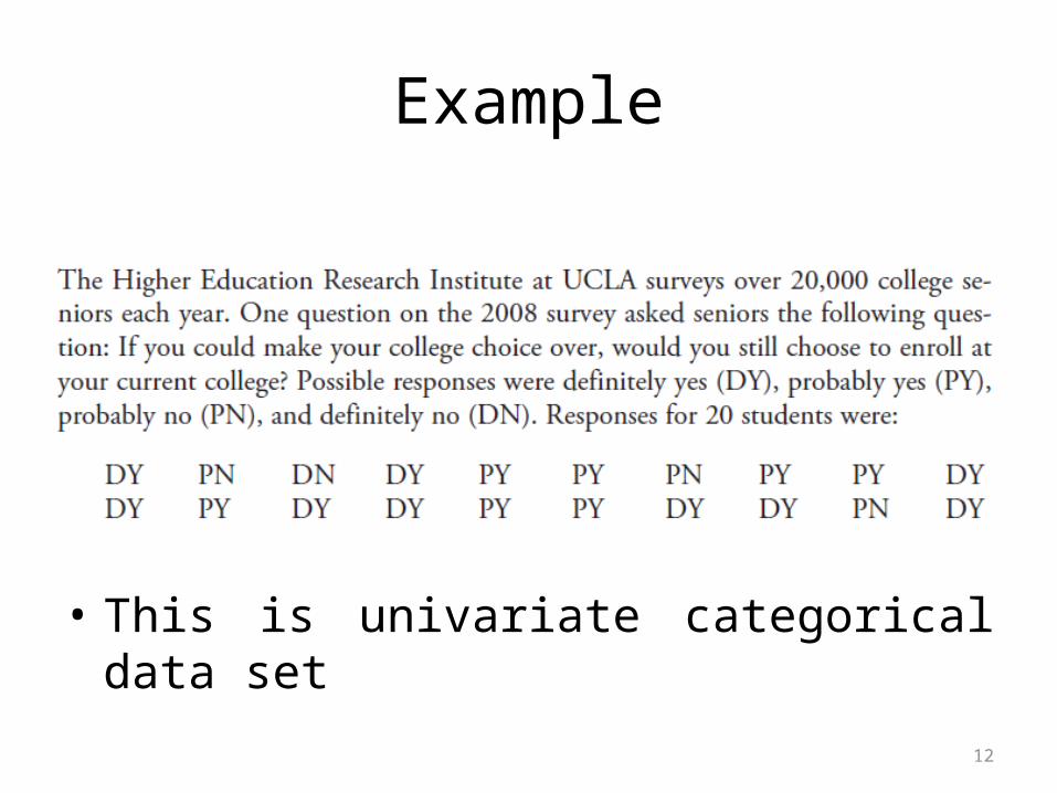
Example

• This is univariate categorical data set

13

Multivariate data

• This is called a bivariate data set. Multivariate data result from obtaining a category or value for each of two or more attributes (so bivariate data are a special case of multivariate data).

• For example, multivariate data would result from determining height, weight, pulse rate, and systolic blood pressure for each individual in a group.

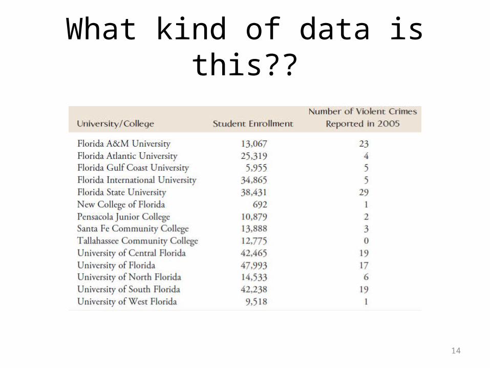
14

What kind of data is this??

15

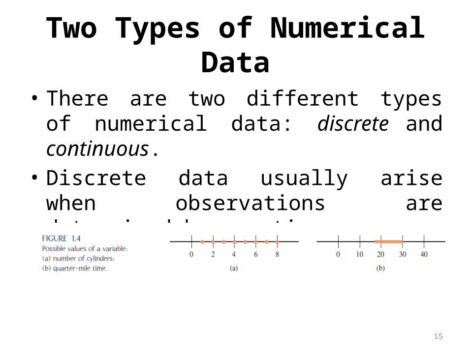
Two Types of Numerical Data

• There are two different types of numerical data: discrete and continuous.

• Discrete data usually arise when observations are determined by counting

16

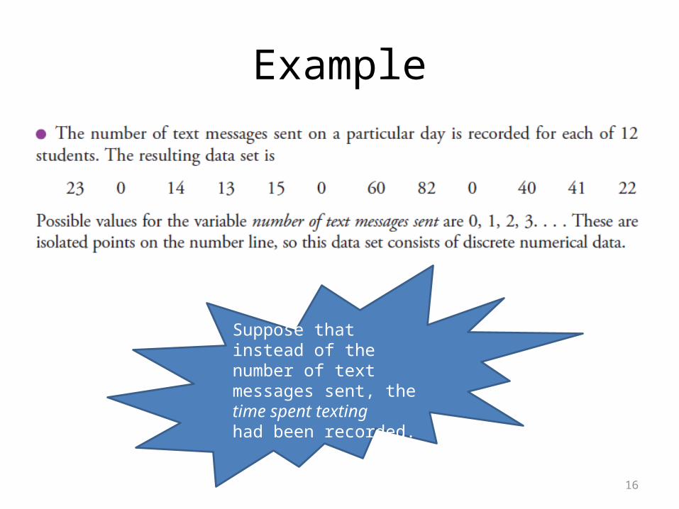
Example

Suppose that instead of the number of text messages sent, the time spent textinghad been recorded.

17

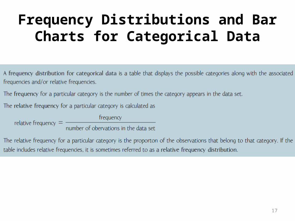
Frequency Distributions and Bar Charts for Categorical Data

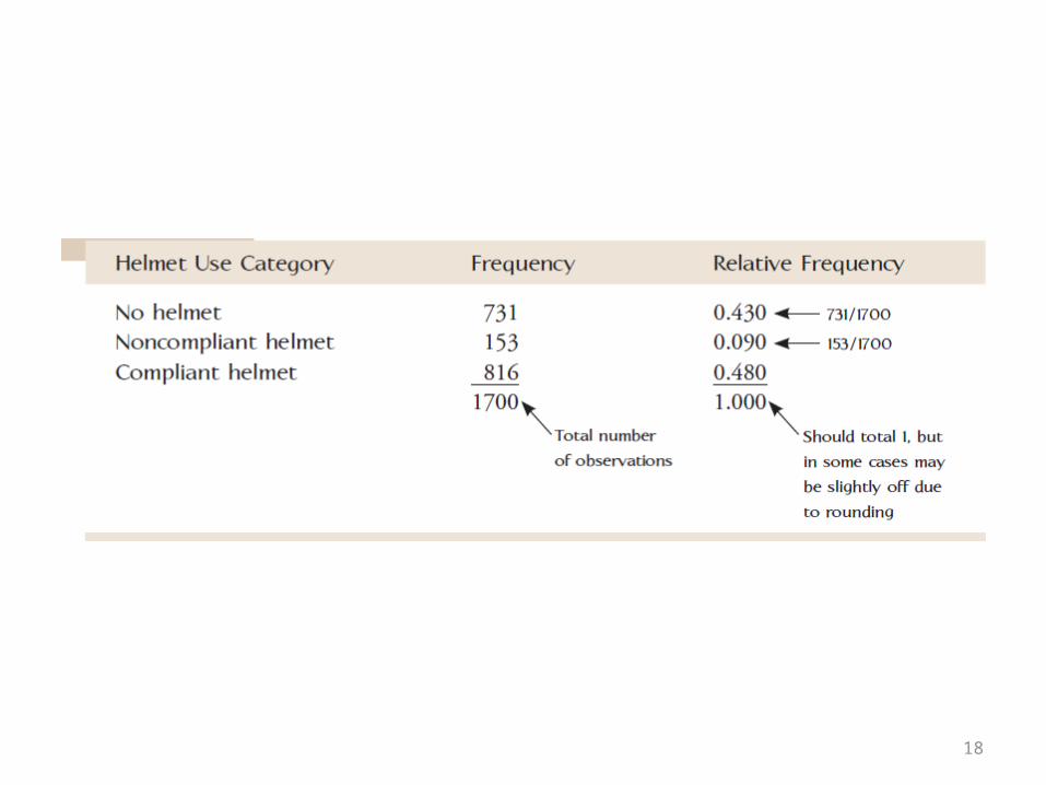
18

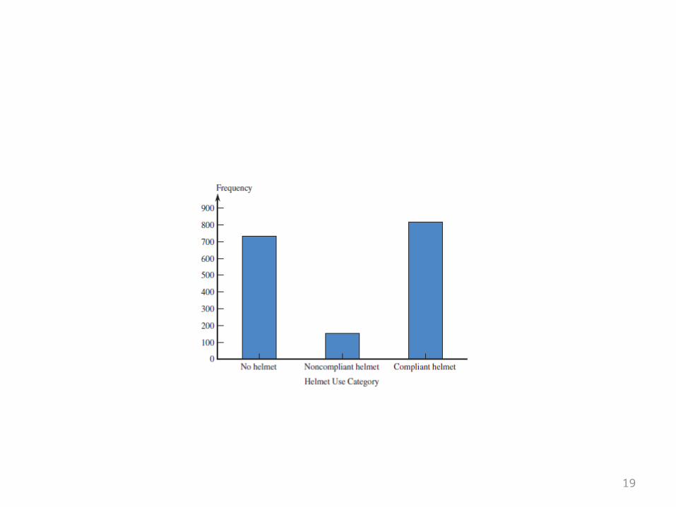
19

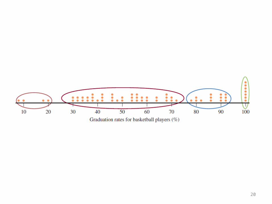
20

21

22

Displaying categorical data : Comparing pie chart with bar chart

• When constructing a comparative bar chart we use the relative frequency rather than the frequency to construct the scale on the vertical axis so that we can make meaningful comparisons even if the sample sizes are not the same.

23

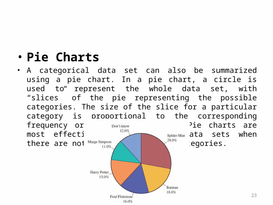
• Pie Charts• A categorical data set can also be summarized using a pie chart. In a pie

chart, a circle is used to represent the whole data set, with “slices” of the pie representing the possible categories. The size of the slice for a particular category is proportional to the corresponding frequency or relative frequency. Pie charts are most effective for summarizing data sets when there are not too many different categories.

24

25

26

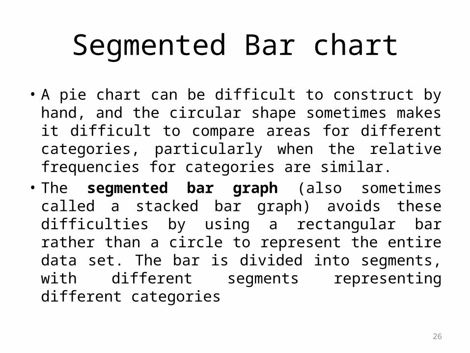
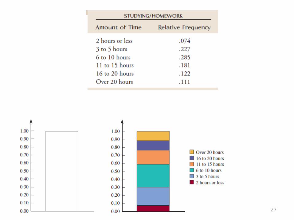
Segmented Bar chart

• A pie chart can be difficult to construct by hand, and the circular shape sometimes makes it difficult to compare areas for different categories, particularly when the relative frequencies for categories are similar.

• The segmented bar graph (also sometimes called a stacked bar graph) avoids these difficulties by using a rectangular bar rather than a circle to represent the entire data set. The bar is divided into segments, with different segments representing different categories

27

28

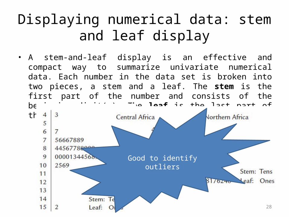
Displaying numerical data: stem and leaf display

• A stem-and-leaf display is an effective and compact way to summarize univariate numerical data. Each number in the data set is broken into two pieces, a stem and a leaf. The stem is the first part of the number and consists of the beginning digit(s). The leaf is the last part of the number and consists of the final digit(s).

Good to identify outliers

29

Frequency Distributions and Histograms for Continuous Numerical Data

30

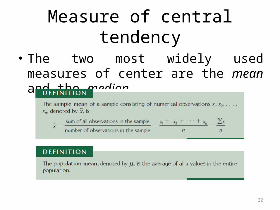
Measure of central tendency

• The two most widely used measures of center are the mean and the median.

31

32

33

34

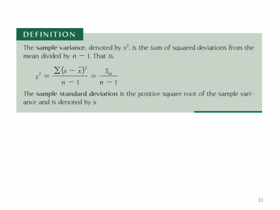
• These measures are called the population variance and the population standard deviation and are denoted by and µ , respectively. (We again use a lowercase Greek letter for a population characteristic.)