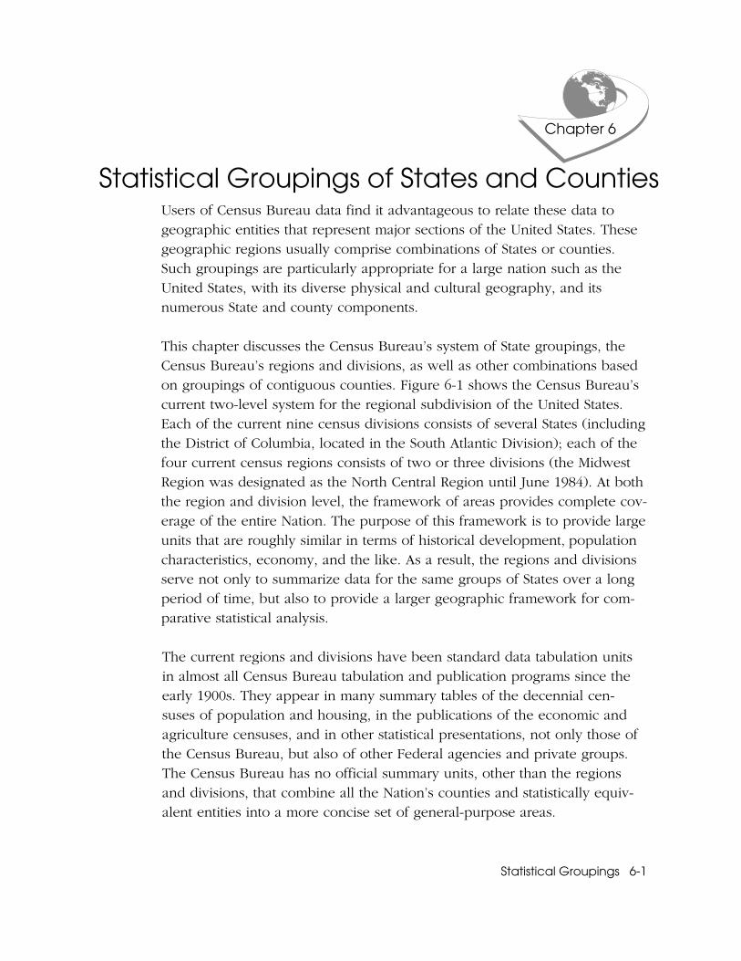
Users of Census Bureau data find it advantageous to relate these data togeographic entities that represent major sections of the United States. Thesegeographic regions usually comprise combinations of States or counties. Such groupings are particularly appropriate for a large nation such as theUnited States, with its diverse physical and cultural geography, and itsnumerous State and county components.

This chapter discusses the Census Bureau’s system of State groupings, theCensus Bureau’s regions and divisions, as well as other combinations basedon groupings of contiguous counties. Figure 6-1 shows the Census Bureau’scurrent two-level system for the regional subdivision of the United States.Each of the current nine census divisions consists of several States (includingthe District of Columbia, located in the South Atlantic Division); each of thefour current census regions consists of two or three divisions (the MidwestRegion was designated as the North Central Region until June 1984). At boththe region and division level, the framework of areas provides complete cov-erage of the entire Nation. The purpose of this framework is to provide largeunits that are roughly similar in terms of historical development, populationcharacteristics, economy, and the like. As a result, the regions and divisionsserve not only to summarize data for the same groups of States over a longperiod of time, but also to provide a larger geographic framework for com-parative statistical analysis.

The current regions and divisions have been standard data tabulation units in almost all Census Bureau tabulation and publication programs since theearly 1900s. They appear in many summary tables of the decennial cen-suses of population and housing, in the publications of the economic andagriculture censuses, and in other statistical presentations, not only those ofthe Census Bureau, but also of other Federal agencies and private groups.The Census Bureau has no official summary units, other than the regions and divisions, that combine all the Nation’s counties and statistically equiv-alent entities into a more concise set of general-purpose areas.

Statistical Groupings 6-1

Statistical Groupings of States and Counties

Chapter 6

6-2 Statistic

al G

rou

pin

gs

Figure 6-1. Census Regions and Divisions of the United States

Statistical Groupings 6-3

Historical PerspectiveThe recognition of geographic regions goes back to the colonial periodof American history. By the 18th century, the names New England, theMiddle Colonies, and the South had come to refer to major sections ofthe Atlantic seaboard. Each of these regions encompassed several adja-cent colonies or areas of settlement. The regional designations reflectedparticularities of location, climate, topography, economic systems, eth-nic composition of the settlers, and systems of local government. Oneearly use of these areas in a statistical compilation dates from before theAmerican Revolution, when the British Government grouped the NorthAmerican colonies into major colonial regions to summarize foreigntrade information. These regions were New England, Middle Colonies,Upper South, and Lower South.

These colonial groupings were the forerunners of the State combina-tions that appear in the census publications. In fact, the area called NewEngland in colonial times has maintained its geographic identity to thepresent day. Much the same is true of the Middle Colonies; except forDelaware, which is now in the Census Bureau’s South Atlantic Division,New Jersey, New York, and Pennsylvania remain the component Statesof the Middle Atlantic Division. (Maryland and Virginia constituted theUpper South; North Carolina, South Carolina, and Georgia, the LowerSouth.) On a smaller scale, there were other regional designations thatappeared in the geographic structure of later censuses; names such astidewater, coastal plain, piedmont, and the back country were knownand in general use even before the American Revolution. These group-ings were of interest from the standpoint of statistical presentationsbecause they referred to relatively homogeneous subareas within sev-eral colonies (or States). Such geographic subdivisions appeared inseveral U.S. publications, often as county groupings that representedareas having similar physical and socioeconomic characteristics.

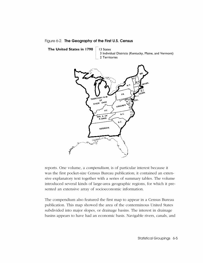
Regional Designations in Early U.S. CensusesAlthough 13 States were in place by the time of the first U.S. census in1790, they were treated as judicial districts in census publications and

6-4 Statistical Groupings

for purposes of data collection. The published data made no use of Statecombinations. Instead, the summary table listed the 13 States (Connecticut,Delaware, Georgia, Maryland, Massachusetts, New Hampshire, New Jersey,New York, North Carolina, Pennsylvania, Rhode Island, South Carolina,and Virginia) and three districts (Kentucky, Maine, and Vermont) underone heading, “Districts.” Two territories (Territory Northwest of RiverOhio, and Territory South of River Ohio) also were under the heading of“Districts” but below the grand totals for the 16 areas listed above.

In 1790, U. S. marshals conducted the decennial census within judicial dis-tricts (this method of enumeration continued until 1870) while TerritorySouth of River Ohio was enumerated by the Governor. Indian warfareprevented the 1790 enumeration of Territory Northwest of River Ohio.Figure 6-2 shows the major geographic entities of the first U.S. Census.

With one exception, the published returns of the 1790 census did notuse any geographic combinations of counties within States; the listingof counties within States was alphabetical, with minor civil divisions andsome incorporated places appearing in similar sequence. The table forMaryland was the exception; it arranged the county totals by westernshore and eastern shore. Although the geographic pattern of the Statesand territories shifted frequently over the next half-century, decennialcensus publications from 1800 to 1840 made no use of large-area sum-mary units. In general, States were listed in geographic order, beginningwith Maine.

The 1850 CensusThe 1850 decennial census brought considerable change to the enumera-tion process and the tabular presentation of statistical compilations. Thepublished reports received the attention of the well-known editor, jour-nalist, and statistician, James D. B. DeBow, who became the Superintend-ent of the Census in 1853. He directed the statistical compilations of the1850 decennial census and completed the publication of several printed

Statistical Groupings 6-5

Figure 6-2. The Geography of the First U.S. Census

The United States in 1790 13 States3 Individual Districts (Kentucky, Maine, and Vermont)2 Territories

reports. One volume, a compendium, is of particular interest because itwas the first pocket-size Census Bureau publication; it contained an exten-sive explanatory text together with a series of summary tables. The volumeintroduced several kinds of large-area geographic regions, for which it pre-sented an extensive array of socioeconomic information.

The compendium also featured the first map to appear in a Census Bureaupublication. This map showed the area of the conterminous United Statessubdivided into major slopes, or drainage basins. The interest in drainagebasins appears to have had an economic basis. Navigable rivers, canals, and

6-6 Statistical Groupings

overland railways were important elements in the Nation’s transportationand communication systems; the network of canals and railroads existing atthe time, along with the plans for expansion of these networks, dependedon drainage and topography as well as the population settlement pattern.This map and the several geographic divisions in the accompanying tableserved as the framework for summarizing the population totals from thefirst seven decennial censuses. This was the first time that a decennial cen-sus publication depicted large-area regions that combined entire Statesand territories (or portions of them) into summary units.

This publication is significant in that numerous statistical tables are pre-sented using the five great divisions, the first set of standard geographicgroupings to appear in a U.S. census publication. Some divisions consistedof several States, others of several States and territories. A more significantfact is that some of the divisions are quite similar to the current census divi-sions. New England still encompasses the same six States. With the excep-tion of Delaware, the District of Columbia, and Maryland, the Middle Statesof 1850 correspond to the present Middle Atlantic Division. With the addi-tion of these same three areas, today’s South Atlantic Division correspondsto the 1850 Southern Division (see Figure 6-3).

Although the 1850 compendium made extensive use of the five great divi-sions, DeBow was not satisfied, because Kentucky and Missouri were sepa-rated from Tennessee and Arkansas and included with the NorthwesternDivision associated with California, Oregon, and the other territories. Insearch of a better set of areas, DeBow devised a new geographic arrange-ment for future use. This classification divided the country into threegreat sections: (1) the Eastern on the Atlantic Coast; (2) the Western onthe Pacific Coast; and (3) the Interior, encompassing the States of Ala-bama, Arkansas, Illinois, Indiana, Iowa, Kentucky, Louisiana, Michigan,Mississippi, Missouri, Ohio, Tennessee, Texas, Wisconsin; the territoriesof Kansas, Minnesota, Nebraska; and the Unorganized Territory of Okla-homa (see Figure 6-3).

Statistical Groupings 6-7

Figure 6-3. The 1850 Groupings and DeBow’s Suggested Rearrangement

The Five Great Divisions of the 1850 Census Compendium (1850 Areas/Boundaries)

Three Great Sections Proposed for Census Use by DeBow (1854 Areas/Boundaries)

6-8 Statistical Groupings

Each great section had its own north and south divisions, designated asNortheastern, Southeastern, Northern Interior, Southern Interior, North-west, and Southwest. In effect, DeBow’s system was a sweeping new geo-graphic arrangement that restated the three major drainage areas: (1) theAppalachian or Atlantic; (2) the Mississippi Valley or Central; and (3) thePacific or Western, as combinations of entire States, or of entire Statesand territories.

In many respects, DeBow’s great sections and divisions anticipated thepresent arrangement of census regions and divisions (see Figure 6-1). TheNorthern Division of the Eastern Section is today’s Northeast Region, theSouthern Division of the Eastern Section comprises the present SouthAtlantic Division, the Southern Interior corresponds largely to today’sEast and West South Central Divisions, the Northern Interior resemblesthe Midwest Region, and the name Western Section still applies to muchthe same area now referred to as the West.

Geographic Summaries for the 1850 and 1860 CensusesOther tables (and consequently maps) from the 1850 and 1860 censusesarranged the States differently than the 1850 compendium. Map A inFigure 6-4 depicts the arrangement of States into sections or groupsaccording to geographical situation, production, climate, the pursuits ofthe inhabitants, and other prominent characteristics. Texas, the CentralSlave States, and the Coast Planting States approximated the South. Thesethree sections corresponded to DeBow’s Southeast and Southern Inter-ior, excluding the District of Columbia, Delaware, and Maryland. Someaspects of the sections or groups presented a rather unusual arrangement;for instance, the Middle States of the Atlantic seaboard also included Ohio,and the designation Northwestern States (often including all the territories)appears to be somewhat lacking in geographic precision. On an overallbasis, the arrangement probably proved less versatile than the five divi-sions of the 1860 census. It appeared only once in the 1850 publication,and was featured in one historical table in the 1860 summary volume.

Statistical Groupings 6-9

The summary tables in the 1860 census publication presented a differentapproach to large-area combinations. Map B in Figure 6-4 shows the stand-ard grouping as a general-purpose arrangement into five divisions, whichappeared in a number of statistical tables on agriculture and manufacturing.Two of the divisions, New England and the Middle States, were identical tothe official Great Divisions of 1850 (see Figure 6-3). One innovation of thispublication was the use of the word Western (in the Western Division)instead of Northwest to designate the interior part of the Nation; anotherwas the name Pacific, appearing for the first time to designate a combina-tion of States.

Another grouping of States (Map C in Figure 6-4) appeared in a specializedtable of railroad mileage and costs. This arrangement made some changes tothe framework of the five 1860 divisions. It combined Arkansas, Kentucky,and Tennessee into Interior South; it retitled much of the Western Divisionas Interior North; and it subdivided the remainder of the Southern Divisioninto Southern Atlantic and Gulf. New England and the Middle Divisions didnot change.

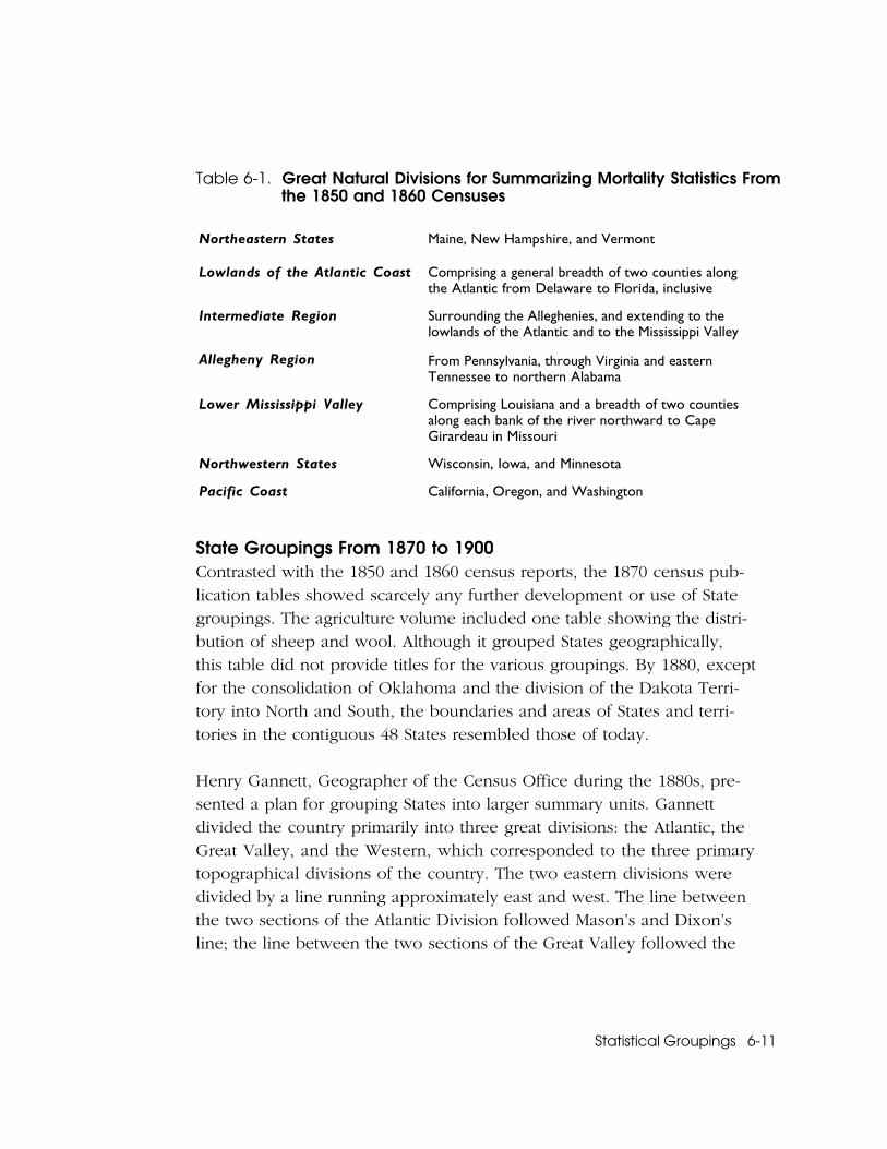
The 1850 and 1860 censuses involved a general enumeration of annualdeaths; the compilations appeared in several tables of mortality statisticsthat featured various kinds of large-area summary units. One table on mor-tality statistics used seven natural divisions for comparing 1850 and 1860information. This approach summarized information on the basis of thephysical aspects of the country (see Table 6-1). The geographic coverageis selective and includes only part of the Nation. Some categories repre-sent groups of entire States (Pacific Coast, Northeastern, and Northwest-ern States), while others refer to groups of counties or parts of States.This regional categorization reflected a continuation of DeBow’s attemptsto divide the Nation into natural regions, albeit from a different perspec-tive. The use of counties as building blocks cumulating to larger geographicareas foreshadowed later efforts in statistical and map presentations in the1870, 1880, 1890, and 1900 censuses.

6-10 Statistical Groupings

Figure 6-4. Other Groupings of States from the 1850 and 1860 Censuses

A. Groupings for Land Area, Population, and Density Table (1850/1860)

B. Five Divisions Used in Many Summary Tables (1860)

C. Areas for Summarizing Railroad Mileage and Costs (1860)

Source: Preliminary Report on the Eighth Census, 1862.

Statistical Groupings 6-11

Table 6-1. Great Natural Divisions for Summarizing Mortality Statistics Fromthe 1850 and 1860 Censuses

Northeastern States Maine, New Hampshire, and Vermont

Lowlands of the Atlantic Coast Comprising a general breadth of two counties alongthe Atlantic from Delaware to Florida, inclusive

Intermediate Region Surrounding the Alleghenies, and extending to thelowlands of the Atlantic and to the Mississippi Valley

Allegheny Region From Pennsylvania, through Virginia and easternTennessee to northern Alabama

Lower Mississippi Valley Comprising Louisiana and a breadth of two countiesalong each bank of the river northward to CapeGirardeau in Missouri

Northwestern States Wisconsin, Iowa, and Minnesota

Pacific Coast California, Oregon, and Washington

State Groupings From 1870 to 1900Contrasted with the 1850 and 1860 census reports, the 1870 census pub-lication tables showed scarcely any further development or use of Stategroupings. The agriculture volume included one table showing the distri-bution of sheep and wool. Although it grouped States geographically,this table did not provide titles for the various groupings. By 1880, exceptfor the consolidation of Oklahoma and the division of the Dakota Terri-tory into North and South, the boundaries and areas of States and terri-tories in the contiguous 48 States resembled those of today.

Henry Gannett, Geographer of the Census Office during the 1880s, pre-sented a plan for grouping States into larger summary units. Gannettdivided the country primarily into three great divisions: the Atlantic, theGreat Valley, and the Western, which corresponded to the three primarytopographical divisions of the country. The two eastern divisions weredivided by a line running approximately east and west. The line betweenthe two sections of the Atlantic Division followed Mason’s and Dixon’sline; the line between the two sections of the Great Valley followed the

6-12 Statistical Groupings

Ohio River and the southern boundary of Missouri. The east-west line sep-arated districts that were very sharply distinguished from one another bypopulation, social conditions, and interests, as well as climate.

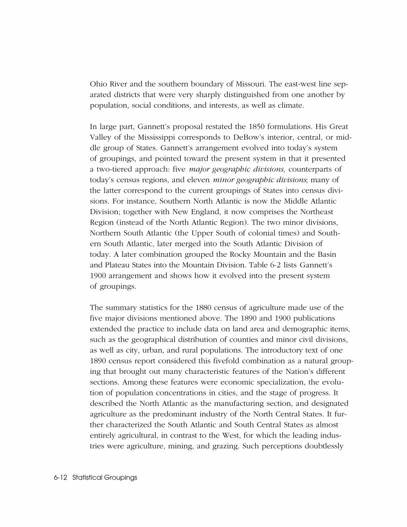
In large part, Gannett’s proposal restated the 1850 formulations. His GreatValley of the Mississippi corresponds to DeBow’s interior, central, or mid-dle group of States. Gannett’s arrangement evolved into today’s systemof groupings, and pointed toward the present system in that it presenteda two-tiered approach: five major geographic divisions, counterparts oftoday’s census regions, and eleven minor geographic divisions; many ofthe latter correspond to the current groupings of States into census divi-sions. For instance, Southern North Atlantic is now the Middle AtlanticDivision; together with New England, it now comprises the NortheastRegion (instead of the North Atlantic Region). The two minor divisions,Northern South Atlantic (the Upper South of colonial times) and South-ern South Atlantic, later merged into the South Atlantic Division oftoday. A later combination grouped the Rocky Mountain and the Basinand Plateau States into the Mountain Division. Table 6-2 lists Gannett’s1900 arrangement and shows how it evolved into the present systemof groupings.

The summary statistics for the 1880 census of agriculture made use of thefive major divisions mentioned above. The 1890 and 1900 publicationsextended the practice to include data on land area and demographic items,such as the geographical distribution of counties and minor civil divisions,as well as city, urban, and rural populations. The introductory text of one1890 census report considered this fivefold combination as a natural group-ing that brought out many characteristic features of the Nation’s differentsections. Among these features were economic specialization, the evolu-tion of population concentrations in cities, and the stage of progress. Itdescribed the North Atlantic as the manufacturing section, and designatedagriculture as the predominant industry of the North Central States. It fur-ther characterized the South Atlantic and South Central States as almostentirely agricultural, in contrast to the West, for which the leading indus-tries were agriculture, mining, and grazing. Such perceptions doubtlessly

Statistical Groupings 6-13

became fixed in the public’s mind, and served to perpetuate the use ofthis set of standard groupings in the Census Bureau’s publications.

The 1883 edition of the Statistical Atlas (privately published as Scribner’sStatistical Atlas of the United States) also used Gannett’s groupings ofStates. The chapter on physical geography has a section on “Natural Group-ing of States,” including a map of the five major geographic divisions. Thechapter on population has a few short tables that group the States by thesegeographic divisions.

Table 6-2. Shifts in the Naming and Arrangement of Regions and Divisions

1880-1890 1900 1910-1940 1950-1990

North Atlantic North Atlantic North NortheastNew England New England New EnglandSouthern North Atlantic Middle Atlantic Middle Atlantic

East North CentralWest North Central

Northern Central North CentralEastern North Central

Midwest (name changedfrom North Central in 1984)

Western North Central East North CentralWest North Central

South Atlantic South AtlanticNorthern South AtlanticSouthern South Atlantic South South

South Atlantic South AtlanticEast South CentralWest South Central

East South CentralWest South Central

South Central South CentralEastern South CentralWestern South Central

Western Western West WestBasin and Plateau Mountain MountainPacif ic Pacif ic Pacif icRocky Mountain

6-14 Statistical Groupings

Groupings of Counties into Physiographic RegionsThe publications for the 1870 through the 1900 census reflected a continu-ing interest in the use of counties as geographic building blocks for regions,particularly those regions based on physiography, topography, drainagebasins, or river systems. Over the period 1850 through 1900, the numberof counties and statistically equivalent entities increased from 1,621 to 2,828;the 1900 layout of county areas and boundaries largely resembled the pres-ent pattern. For census purposes, counties were becoming a stable frame-work of geographic units; this development favored their use as buildingblocks for data tabulation and presentation. They also served the need fora smaller set of geographic units on which to base regional configurations.

The Census Office’s 1874 Statistical Atlas contained a discussion of the phys-ical features of the country, prepared by Professor J. D. Whitney. The atlashad no accompanying statistical tables, but Whitney’s discussion of physi-ographic regions in the text became the basis for a presentation of data byregions based on physical features in the 1880 census report. Before thepublication of the 1874 text in the statistical atlas, the 1850 and 1860 censusmortality tables also made partial use of county groupings as summary areas.

Gannett continued this approach in the 1880, 1890, and 1900 census publi-cations. The 1880 census report presents some summary data by 21 topo-graphic regions, a practice continued in the publications of the 1890 censusand, with minor modifications, the 1900 census as well. The populationreport for 1890 focused extensively on geographic distributions by naturalregions. These included not only demographic statistics by topographicdivisions, but also others: drainage basins, altitude, mean annual tempera-ture, and rainfall. All 1890 census tables contained historical informationfrom 1870 and 1880 recomputed or rearranged to conform to topographicregions and other areas shown in maps from the 1874 Statistical Atlas.The 1900 census publication continued these presentations.

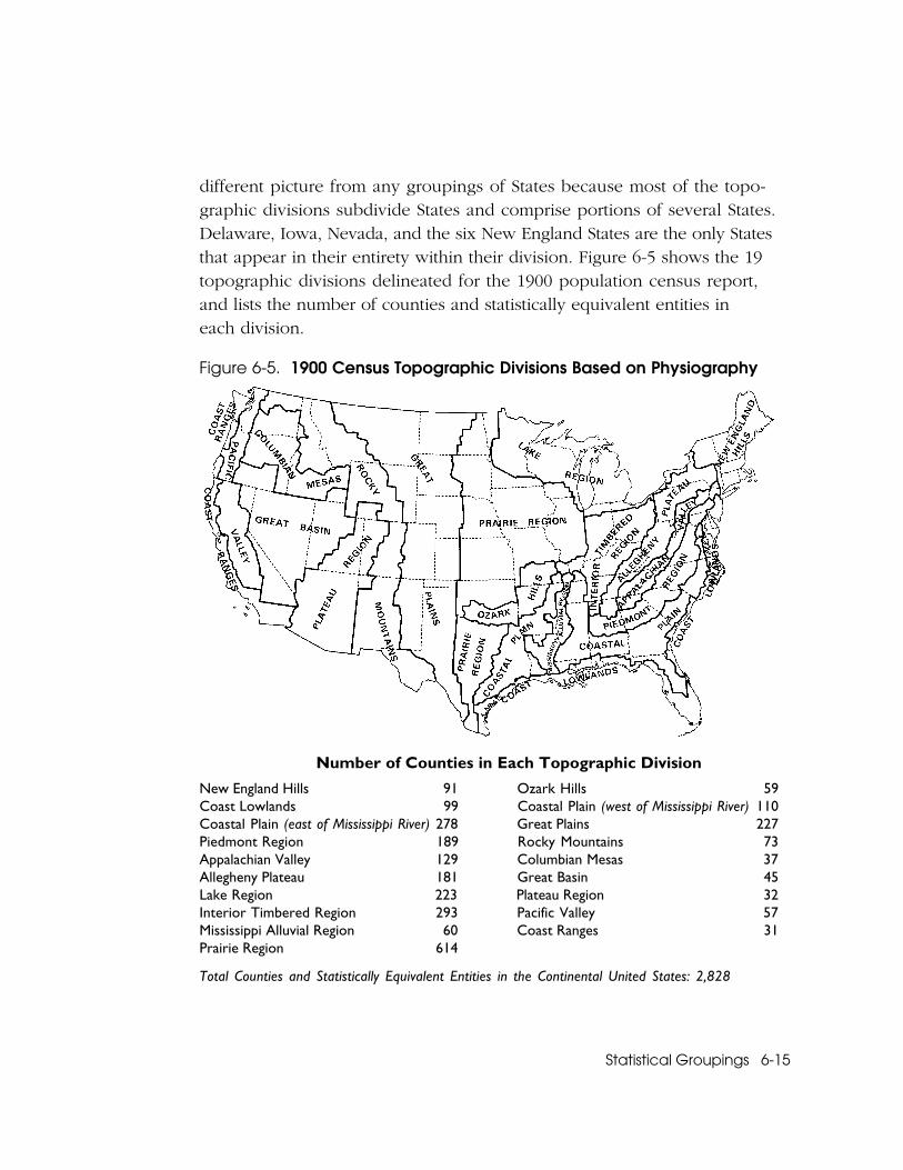
A 1900 census report shows the 19 topographic divisions delineated forthat census, and lists the number of counties and statistically equivalent enti-ties in each division. Geographic arrangements of natural regions present a

Statistical Groupings 6-15

different picture from any groupings of States because most of the topo-graphic divisions subdivide States and comprise portions of several States.Delaware, Iowa, Nevada, and the six New England States are the only Statesthat appear in their entirety within their division. Figure 6-5 shows the 19topographic divisions delineated for the 1900 population census report,and lists the number of counties and statistically equivalent entities ineach division.

Figure 6-5. 1900 Census Topographic Divisions Based on Physiography

Number of Counties in Each Topographic Division

New England Hills 91 Ozark Hills 59Coast Lowlands 99 Coastal Plain (west of Mississippi River) 110Coastal Plain (east of Mississippi River) 278 Great Plains 227Piedmont Region 189 Rocky Mountains 73Appalachian Valley 129 Columbian Mesas 37Allegheny Plateau 181 Great Basin 45Lake Region 223 Plateau Region 32Interior Timbered Region 293 Pacific Valley 57Mississippi Alluvial Region 60 Coast Ranges 31Prairie Region 614

Total Counties and Statistically Equivalent Entities in the Continental United States: 2,828

6-16 Statistical Groupings

A 1900 Census Office bulletin stated that in order for topographic divisionsto serve statistical purposes, the lines between them must coincide withthe boundaries of areas for which statistics are given separately by the cen-sus. Since the smallest available entity at that time was the county, Gannettadjusted the topographic division boundaries to coincide with county lines.To this day, one of the most basic operational rules of the Census Bureau’sgeographic hierarchy is that geographic statistical entities for presentingcensus data must correspond to the geographic units for which the infor-mation otherwise is collected or tabulated. In delineating the divisions, hefound that it was necessary to balance the different variables of geology,topography, altitude, rainfall, and temperature in order to create a physi-cally homogeneous geographic entity enclosed by county boundaries.

Aside from Gannett’s participation in delineating geographic divisions,both for the decennial census publications from 1880 through 1900, andfor historical compilations involving the 1870 statistics by county, hisobservations set forth in the 1900 Census Office bulletin also include themention of geographic splits; that is, the operational subdivision of exist-ing collection units that must serve as the building blocks for some dif-ferent kind of geographic entity in a data tabulation or publication. Thispractice continues in selected census tabulations; for instance, the CensusBureau frequently splits other standard geographic units to provide datafor entities such as incorporated places (see Chapter 9, “Places”).

Stability of State Groupings as Census Summary UnitsBy the late 19th Century, the geographic designations Northeast, South,Interior, and West had come to mean much the same as they do today.This general acceptance undoubtedly favored the retention of the 1880pattern of State groupings in the Census Bureau’s statistical presentationsrather than creating other combinations. Starting with the 1900 census,the statistical tables presented fewer alternative geographic groupings;instead, they made increasing use of a single, standard set of summaryareas. The introductory texts in subsequent publications of the Census

Statistical Groupings 6-17

Bureau tended to be shorter, with fewer presentations or explanationsof other approaches.

The 1880 census grouping of States into divisions and major sectionstherefore became the geographic summary units recognized for all sub-sequent censuses from 1890 through 1990. With some minor modifica-tions, Census Bureau publications used them throughout the first severaldecades of this century to present information from the censuses ofpopulation, agriculture, and industry. The same set of areas also wereused during the 1930s and 1940s for the new censuses of business, con-struction, housing, and services.

The nine divisions as presently constituted, except for Alaska and Hawaii,first appeared in the population report of the 1910 decennial census. Inaddition to divisions, the report contained information for the North,South, and West sections, as well as a separate summary by States eastand west of the Mississippi River. The 1910 Census of Agriculture useda similar arrangement, as did the decennial census of 1920.

The 1930 population and agriculture census publications also used ninegeographic divisions; however, the population census omitted summa-rizing data for the three sections, as well as the designation of areas aseast and west of the Mississippi River. The agriculture census reportscontinued to use the three major sections, North, South, and West. The1940 population and housing census reports revived these three areas;they also continued to present statistics for the nine divisions. The 1950census publications presented summaries for the same nine geographicdivisions in use since 1910. At a higher level, some slight modificationstook place—the use of the name region instead of section, and therearrangement of the four northern divisions that composed the NorthSection into the Northeast and North Central Regions, each consistingof two geographic divisions. The 1960 census saw the addition of Alaskaand Hawaii to the Pacific Division; the 1970 and 1980 census publicationsbrought no further changes. Except for the 1984 renaming of the North

6-18 Statistical Groupings

Central Region as Midwest, the Census Bureau continued the same systemof geographic units for the 1990 census publications.

Publication of Census DataSeveral Census Bureau publications use the regions and divisions to sum-marize data tabulations from the decennial censuses. Among these, themost important reports constitute chapters of major subject-matterfields that summarize population and housing characteristics. Thesereports present summaries of both complete-count and sample datafrom the census of population and housing for the Nation as a whole,as well as data for the regions, divisions, States, urban and rural areas, themetropolitan and nonmetropolitan categories, and the other basic geo-graphic units. In addition, various presentations from the other censusesand sample surveys use regions and divisions as part of their geographicsummary units.

Some Alternate Approaches to State GroupingsAlthough the system of regions and divisions has remained largelyunchanged for many decades, the data user community periodically sug-gests new approaches to large-area summary geography. The CensusBureau, in turn, examines these proposals and considers them as pos-sible improvements to the existing framework of State groupings.

One major review took place after the 1950 census, when an interagencycommittee within the Department of Commerce compared the existingCensus Bureau regions and divisions to other schemes of regionalizationand assessed the usefulness of an alternative system. Because the existingState groupings resulted largely from tradition, with few major changesfrom the 1880 set of summary units, it seemed worthwhile to test thesecombinations by using more modern statistical approaches and tech-niques. The following ground rules guided the study:

• Socioeconomic homogeneity is the principal criterion for groupingStates into regions.

• Each combination should consist of two or more adjacent States.

Statistical Groupings 6-19

• Objective statistical analysis is the primary basis for the classification.

• The number of eventual combinations should range from 6 to 12.

By using various statistical indexes, it was possible to identify almostthree-quarters of the States (34 out of 48) as homogeneous cores of aregion or division. The remaining 14 States proved to be somewhatmarginal; the statistical evidence was less certain; they fell between tworegions and, therefore, could belong to either. It is interesting that theproposed new arrangement contained the same number of groupings(four regions and nine divisions) as the existing system. It retained thesame names for the four regions, but made a number of changes ingrouping the States. The proposal assigned many States that were onthe border of an existing region to a different region, and some toentirely new divisions. For instance, it shifted Delaware, the District ofColumbia, and Maryland from the South Region to the Middle AtlanticDivision of the Northeast Region; it combined Texas, Oklahoma, Ari-zona, and New Mexico to form a Southwest Division within an expandedWest Region; it grouped Nevada with the Pacific States as part of a FarWest Division; and it revamped the South into two divisions, each com-prising an upper and lower tier of States. It renamed all but two divisions(New England and the Middle Atlantic). Only three of the resulting ninedivisions maintained their original State components: (1) New England,(2) the Plains (formerly West North Central), and (3) the Great Lakes(formerly East North Central).

This suggested reclassification had its merits, for on a purely statisticalbasis it provided a more homogeneous set of areas than any others thenin use by the Department of Commerce. However, the new system didnot win enough overall acceptance among data users to warrant adoptionas an official new set of general-purpose State groupings. The previousdevelopment of many series of statistics, arranged and issued over longperiods of time on the basis of the existing State groupings, favored theretention of the summary units of the current regions and divisions (seeFigure 6-1).

6-20 Statistical Groupings

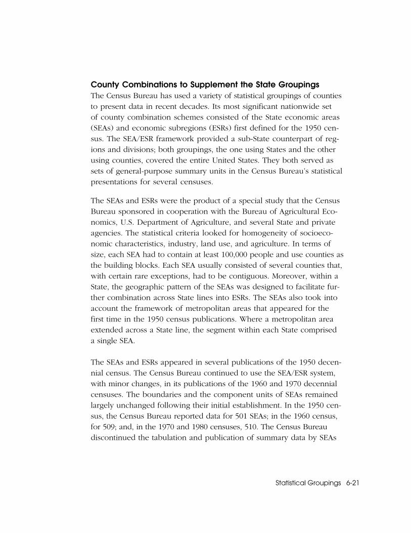
In the 1970s, the Federal Government developed another set of summaryareas for use in statistical presentations based on groupings of States. TheOffice of Management and Budget (OMB) directed the use of StandardFederal Administrative Regions (SFARs) by all Federal agencies that pub-lish regional data. The SFARs consist of ten regions that cover not onlythe 50 States and the District of Columbia, but also Guam, Puerto Rico,and the Virgin Islands of the United States. The resulting geographic pat-tern is quite different from the layout of census regions and divisions;New England is the only instance where the two sets of areas coincide.

The SFAR framework resulted from an OMB survey of State officials thatsought an arrangement of States different from the traditional regionsand divisions. The OMB directive prescribed that Federal agencies pub-lishing data supplied directly by States use the SFARs for such presenta-tions. Other arrangements were permissible, either for special analyticalpurposes or for maintaining the continuity of a historical data series. Onthis basis, the Census Bureau continued to use its system of regions anddivisions in the 1980 and 1990 decennial census publications.

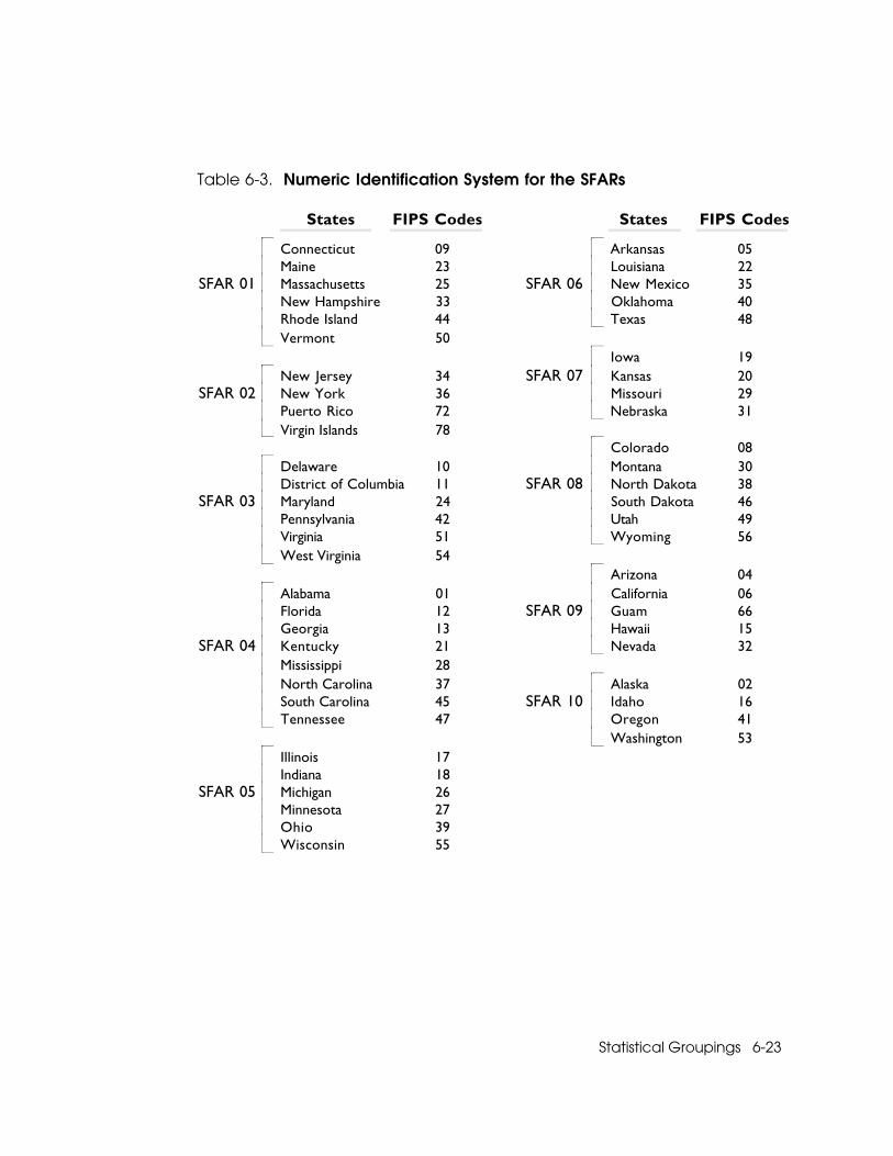
Coding Schemes for State GroupingsTables 6-3 and 6-4 show the numeric schemes for identifying the SFARsand the census regions and divisions. The State identification codes in theSFAR framework are from the Federal Information Processing Standards(FIPS), an official system developed by the National Institute of Standardsand Technology (formerly known as the National Bureau of Standards)and maintained by the U.S. Geological Survey. The FIPS State codes arenumbered in alphabetic sequence. By contrast, the Census Bureau usesa supplementary set of State codes that follow a geographic sequencewithin each census division; this permits processing the 50 States andthe District of Columbia by geographic division. A one-digit code rep-resents each division; the same number appears as the first digit in theCensus Bureau’s two-digit State code. At a separate, higher level, a one-digit code represents each of the four regions.

Statistical Groupings 6-21

County Combinations to Supplement the State GroupingsThe Census Bureau has used a variety of statistical groupings of countiesto present data in recent decades. Its most significant nationwide setof county combination schemes consisted of the State economic areas(SEAs) and economic subregions (ESRs) first defined for the 1950 cen-sus. The SEA/ESR framework provided a sub-State counterpart of reg-ions and divisions; both groupings, the one using States and the otherusing counties, covered the entire United States. They both served assets of general-purpose summary units in the Census Bureau’s statisticalpresentations for several censuses.

The SEAs and ESRs were the product of a special study that the CensusBureau sponsored in cooperation with the Bureau of Agricultural Eco-nomics, U.S. Department of Agriculture, and several State and privateagencies. The statistical criteria looked for homogeneity of socioeco-nomic characteristics, industry, land use, and agriculture. In terms ofsize, each SEA had to contain at least 100,000 people and use counties asthe building blocks. Each SEA usually consisted of several counties that,with certain rare exceptions, had to be contiguous. Moreover, within aState, the geographic pattern of the SEAs was designed to facilitate fur-ther combination across State lines into ESRs. The SEAs also took intoaccount the framework of metropolitan areas that appeared for thefirst time in the 1950 census publications. Where a metropolitan areaextended across a State line, the segment within each State compriseda single SEA.

The SEAs and ESRs appeared in several publications of the 1950 decen-nial census. The Census Bureau continued to use the SEA/ESR system,with minor changes, in its publications of the 1960 and 1970 decennialcensuses. The boundaries and the component units of SEAs remainedlargely unchanged following their initial establishment. In the 1950 cen-sus, the Census Bureau reported data for 501 SEAs; in the 1960 census,for 509; and, in the 1970 and 1980 censuses, 510. The Census Bureaudiscontinued the tabulation and publication of summary data by SEAs

6-22 Statistical Groupings

and ESRs for the 1980 and 1990 censuses as a result of apparent userdisinterest in this information.

Finally, the Census Bureau uses one other approach that combines coun-ties. This county grouping is of the Census Bureau’s public-use microdatasamples (PUMS). The PUMS data product differs from the standardprinted reports, computer tapes, microfiche, and the like, that presentstatistical summaries of all responses, either of complete-count informa-tion or of information collected from only a sample of households. Bycontrast, the PUMS files use a sample of raw data for areas of 100,000 orgreater population; PUMS areas typically comprise large cities, group-ings of counties, or remainders of counties. From these samples, thedata users can select and manipulate specific responses to create custo-mized decennial census tabulations in much the same way as if they hadcollected the information in their own census or sample survey. Strictlyspeaking, the PUMS microdata areas are not official geographic units, asthe Census Bureau provides neither totals nor summary information forthem. Instead, they are part of an ad hoc geographic framework estab-lished for data users who wish to analyze the diverse relationships amongresponses to standard questions.

Proposals for Changes in the FutureAs geographic combinations, the regions and divisions are familiar withinthe data user community. The Census Bureau intends to continue prepar-ing data tabulations for these entities as standard parts of its tabulation andpublication programs in future decennial censuses of population and hous-ing, its quinquennial agricultural and economic censuses, its many currentsample surveys, and its other compilations and compendia. As part of itscontinuing effort to improve the definition and delineation of geographicareas for each decennial census, the Census Bureau’s Statistical Areas Com-mittee will review the components of the regions and divisions to ensurethat they continue to represent the most useful combinations of Statesand State equivalents.

Statistical Groupings 6-23

Table 6-3. Numeric Identification System for the SFARs

States FIPS Codes States FIPS Codes

Connecticut 09 Arkansas 05Maine 23 Louisiana 22

SFAR 01 Massachusetts 25 SFAR 06 New Mexico 35New Hampshire 33 Oklahoma 40Rhode Island 44 Texas 48Vermont 50

Iowa 19New Jersey 34 SFAR 07 Kansas 20

SFAR 02 New York 36 Missouri 29Puerto Rico 72 Nebraska 31Virgin Islands 78

Colorado 08Delaware 10 Montana 30District of Columbia 11 SFAR 08 North Dakota 38

SFAR 03 Maryland 24 South Dakota 46Pennsylvania 42 Utah 49Virginia 51 Wyoming 56West Virginia 54

Arizona 04Alabama 01 California 06Florida 12 SFAR 09 Guam 66Georgia 13 Hawaii 15

SFAR 04 Kentucky 21 Nevada 32Mississippi 28North Carolina 37 Alaska 02South Carolina 45 SFAR 10 Idaho 16Tennessee 47 Oregon 41

Washington 53Illinois 17Indiana 18

SFAR 05 Michigan 26Minnesota 27Ohio 39Wisconsin 55

6-24 Statistical Groupings

Table 6-4. Census Codes for Regions and Divisions

Division 1: New England Division 2: Middle AtlanticMaine 11 New York 21New Hampshire 12 New Jersey 22

Region 1: Vermont 13 Pennsylvania 23Northeast Massachusetts 14

Rhode Island 15Connecticut 16

Division 3: East North Central Division 4: West North CentralOhio 31 Minnesota 41

Region 2: Indiana 32 Iowa 42Midwest* Illinois 33 Missouri 43

Michigan 34 North Dakota 44Wisconsin 35 South Dakota 45

Nebraska 46Kansas 47

Division 5: South Atlantic Division 6: East South CentralDelaware 51 Kentucky 61Maryland 52 Tennessee 62District of Columbia 53 Alabama 63

Region 3: Virginia 54 Mississippi 64South West Virginia 55

North Carolina 56 Division 7: West South Central

South Carolina 57 Arkansas 71Georgia 58 Louisiana 72Florida 59 Oklahoma 73

Texas 74

Division 8: Mountain Division 9: PacificMontana 81 Washington 91Idaho 82 Oregon 92Wyoming 83 California 93

Region 4: Colorado 84 Alaska 94West New Mexico 85 Hawaii 95

Arizona 86Utah 87Nevada 88

*The Midwest Region was designated as the North Central Region until June 1984.

Statistical Groupings 6-25

The Census Bureau keeps abreast of new concepts and approaches, andweighs their possible use in its geographic hierarchy for data presenta-tions. New geographic designations appear frequently, and a few find theirway into public usage. Although the names Sunbelt, Frostbelt, and Rustbelthave found favor in some quarters, these terms often mean one particularcombination of States (and sometimes, counties) to some people and adifferent combination of States and counties to others. Moreover, the per-ception of regions can shift in terms of both names and boundaries withchanging circumstances; today’s Energy Belt may be tomorrow’s Oil BustBelt. Such geographic combinations appear to fit, more properly, intospecial, one-of-a-kind statistical tabulations that some data users requestfrom a particular census or survey. The Census Bureau sometimes usessuch large-area regions to meet the particular needs of special data presen-tations. Examples are travel regions, which are groupings of States, andoil and gas districts, which represent combinations of selected produc-ing counties. Also, the Census Bureau always is ready to provide specialtabulations, at cost, for almost any set of geographic combinations datausers may request. However, the acceptance of new general-purposegeographic regions by the Census Bureau hinges upon an overall favor-able consensus of the data user community regarding a long-standingset of statistical entities.