Statistical-Empirical Modelling of Airfoil Noise Subjected to

Leading Edge Serrations

Till M. Biedermann1

ISAVE, Duesseldorf University of Applied Sciences, Duesseldorf, D-40474, Germany

Tze Pei Chong2

Department of Mechanical, Aerospace and Civil Engineering, Brunel University London, Uxbridge, UB8 3PH,

United Kingdom

Frank Kameier3

ISAVE, Duesseldorf University of Applied Sciences, Duesseldorf, D-40474, Germany

and

Christian O. Paschereit4

Berlin Technical University, Berlin, D-10623, Germany

With the objective of reducing the broadband noise from the interaction of highly

turbulent flow and airfoil leading edge, sinusoidal leading edge serrations were investigated

as an effective passive treatment. An extensive aeroacoustic study was performed in order to

determine the main influences and interdependencies of factors, such as the Reynolds

number, turbulence intensity, serration amplitude and wavelength as well as the angle of

attack on the noise reduction capability. A statistical-empirical model was developed to

predict the overall sound pressure level and noise reduction of a NACA65(12)-10 airfoil with

and without leading edge serrations in the range of chord-based Reynolds numbers of

2.5·105 ≤ Re ≤ 6·10

5. The observed main influencing factors on the noise radiation were

quantified in a systematic order for the first time. Moreover, significant interdependencies of

the turbulence intensity and the serration wavelength, as well as the serration wavelength

and the angle of attack were observed, validated and quantified. The statistical-empirical

model was validated against an external set of experimental data, which is shown to be

accurate and reliable.

1 Doctoral Researcher, Institute of Sound and Vibration Engineering ISAVE, till.biedermann@hs-duesseldorf.de,

AIAA Student Member 2 Senior Lecturer, Department of Mechanical, Aerospace and Civil Eng., t.p.chong@brunel.ac.uk, AIAA Member

3 Professor, Institute of Sound and Vibration Engineering ISAVE, frank.kameie@hs-duesseldorf.de

4 Professor, Institute of Fluid Dynamics and Technical Acoustics ISTA, oliver.paschereit@tu-berlin.de

Nomenclature

A = amplitude of leading edge serrations [mm]

λ = wavelength of leading edge serrations [mm]

U0 = free stream velocity [ms-1

]

ρ0 = fluid density [kgm-3

]

c = sound velocity[ms-1

]

Tu = turbulence intensity [%]

Re = chord-based Reynolds number [--]

C = airfoil chord length [mm]

S = airfoil span [mm]

H = nozzle height [mm]

R = observer distance in the far-field [m]

d = maximum airfoil thickness [mm]

AoA = angle of attack [°], equals non-dimensional vertical displacement z/H

x = local streamwise (longitudinal) coordinate [mm]

y = local anti-streamwise (transversal) coordinate [mm]

z = local vertical coordinate [mm]

OASPL = overall sound pressure level [dB]

ΔOASPL = overall sound pressure level reduction [dB]

SPL = sound pressure level [dB]

ΔSPL = sound pressure level reduction [dB]

f = frequency [Hz]

ω = angular frequency [s-1

]

Θ = polar angle [deg]

Ma = Mach number [--]

LE = leading edge

I. Introduction

ECENT research has firmly established sinusoidal leading edge (LE) serrations as an effective passive

treatment to reduce the broadband noise of an airfoil when exposed to a highly turbulent flow. A reduction in the

overall sound pressure level of up to ΔOASPL = 7 dB and the sound pressure level reductions ΔSPL > 10 dB in the

relevant frequency region could be achieved [1–4]. Although different hypotheses on the noise reduction mechanism

were proposed before, they have hitherto not been comprehensively verified. In general, three mechanisms could be

responsible for the reduction in the broadband noise. First is the reduced spanwise correlation coefficients as a result

of incoherent response times of the incoming turbulence; second, a reduction of the acoustic sources as manifested

in the reduction in pressure fluctuation at the serration peak; and third, a reduction of the streamwise turbulence

intensity due to the converging flow within the serration gaps [5, 6].

Up to now, research on the effect of LE serrations focused either on the noise reduction capability, or on the

aerodynamic performance of the airfoil itself. The effect of sinusoidal LE on the lift and drag forces has been

analyzed experimentally, numerically and through the use of flow pattern visualization [7, 8]. Moreover, a numerical

study to optimize the serration design in order to improve the aerodynamic forces on the airfoil was presented [9].

Of particular importance is the correlation between the aerodynamic flow behaviors and aeroacoustic noise

reduction mechanisms. In general, the incoming turbulence amplifies the surface pressure fluctuations close to the

airfoil LE, which then radiate into broadband noise [10, 11].

Recently, there have been many studies using high-fidelity numerical flow simulation to provide a physical

insight of the noise reduction mechanisms by the serration [12–14]. These studies show that the surface pressure

fluctuation and the far field noise on a serrated leading edge are de-correlated by the serrated LEs. In particular, the

noise source at the mid-region of the oblique edge becomes ineffective across the mid to high frequency range. The

serration could cause a significant decrease in the surface pressure fluctuations around the tip and mid-regions of the

serration and subsequently reduce the broadband noise level. Another noise reduction mechanism is attributed to the

phase interference and destruction effect between the serration peak and the mid-region of the oblique edge.

Accordingly, the serration root could still remain effective in the noise radiation. Interestingly, a small modification

of the serration root has been found to be able to further reduce the LE noise level [15]. The converging nature of the

serration could also generate a nozzle effect to accelerate the flow within and reduce the level of turbulence intensity

before the fluid-structure interaction near the stagnation points. Analytical work also begins to emerge that

R

generalizes Amiet’s theory of leading edge noise to calculate the airfoil response function subjected to serrated LEs

of different serration wavelengths and amplitudes and the far field noise radiation [16]. Although the analytical

model can predict the acoustic power spectral densities that match reasonably well with the experimental results [1],

the requirement of the iterative solving procedure to calculate the gust response function of the appropriate order

makes it not straightforward to use. This paper aims to generalize the airfoil noise subjected to LE serrations by

developing a statistical–empirical model.

Several parameters have been found to influence the effectiveness of noise reduction by LE serrations, which

include the Reynolds number (Re), turbulence intensity (Tu), serration amplitude (A/C), serration wavelength (λ/C)

and angle of attack (AoA). However, up to now, these parameters have been investigated independently, and only

little effort was made to analyze them as an interrelated system of factors with respect to the noise reduction. This

serves as motivation for the current work, where a comprehensive statistical–empirical model has been developed

with the aim to describe the noise radiation of serrated LEs as an interrelated system involving the aforementioned

five influencing parameters. Note that the current model does not predict the acoustic spectral characteristics for

individual airfoil of serrated leading edges. Rather, the target value describing the noise radiation and noise

reduction by the LE serrations is defined as the Overall Sound Pressure Level (OASPL).

II. Experimental Setup

In the current study, a cambered NACA65(12)-10 airfoil was chosen due to its relevance in the real-life

application such as the stator vanes or axial fan blades. As shown in Fig. 1, the airfoil has a chord length of C = 150

mm and a span width of S = 300 mm. The airfoil geometry consists a removable frontal part (0 < x/C < 0.3) that

allows various LE serration profiles to be attached. Once attached to the rear part main body, the serrations give the

appearance that they are cut into the airfoil’s main body. Therefore the maximum chord is always held constant at C

= 150 mm for all the configurations [2]. The serration geometries are predominantly defined by their amplitude

(chordwise peak-to-trough value) and wavelength (spanwise peak-to-peak-value). Both parameters would be

normalized by the airfoil chord length throughout the paper. The shape of the LE serrations is designed according to

a sinusoidal curve, and the NACA65(12)-10 profile was extruded along the line of this curve. An important feature

of the current design is the semi-cyclic shape of the serration tips as depicted in Fig. 1.

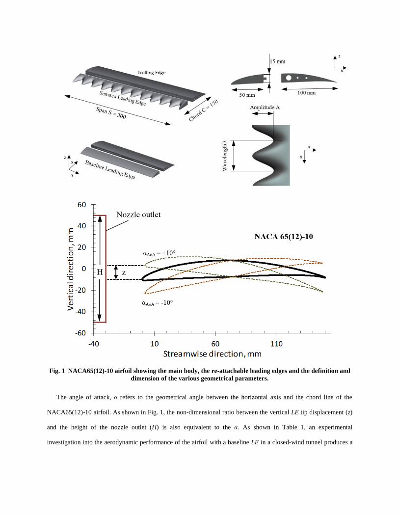
Fig. 1 NACA65(12)-10 airfoil showing the main body, the re-attachable leading edges and the definition and

dimension of the various geometrical parameters.

The angle of attack, α refers to the geometrical angle between the horizontal axis and the chord line of the

NACA65(12)-10 airfoil. As shown in Fig. 1, the non-dimensional ratio between the vertical LE tip displacement (z)

and the height of the nozzle outlet (H) is also equivalent to the α. As shown in Table 1, an experimental

investigation into the aerodynamic performance of the airfoil with a baseline LE in a closed-wind tunnel produces a

lift coefficient, CL = 0.64 at α = 0o. The airfoil was attached to the side-plates extending from both sides of the

nozzle outlet.

A pivot-mounted insert of the side-plates facilitates accurate rotation of the airfoil between α = ± 10o. Due to the

relatively low value of H in the current nozzle, measurement beyond α = ± 10o was not attempted. Note that no

correction of the free jet deflection was applied in the current study. Therefore, it is more effective to use the non-

dimensional quantity of z/H to represent the angle-alignment between the incoming mean flow and the airfoil

leading edge instead of the geometrical angle α.

Table 1 Coefficients of lift, drag and lift-to-drag ratio at z/H = 0 and Re = 250,000. Measurements took

place at the closed wind tunnel at Brunel University London.

A/C λ/C CL CD CL/CD

BSLN -- -- 0.637 0.0342 18.62

A29λ26 0.19 0.17 0.550 0.0336 16.37

A22λ18 0.12 0.12 0.540 0.0338 15.95

A35λ18 0.23 0.12 0.566 0.0356 15.91

A22λ34 0.12 0.23 0.521 0.0330 15.79

A35λ34 0.23 0.23 0.564 0.0325 17.36

A12λ26 0.08 0.17 0.539 0.0335 16.06

A45λ26 0.30 0.17 0.497 0.0330 15.07

A29λ7.5 0.19 0.05 0.478 0.0363 13.16

A29λ45 0.19 0.30 0.586 0.0309 18.97

The noise experiments took place at the open jet wind tunnel of the aeroacoustic facility at Brunel University

London. The exit nozzle, which has a dimension of 100 mm x 300 mm, is situated inside a semi-anechoic chamber

(4.0 m x 5.0 m x 3.4 m). It can produce a typical turbulence intensity of between 0.1 % and 0.2 % [17, 2]. The

maximum jet velocity is about 80 ms-1

. In order to generate elevated turbulence intensities (Tu) at the freestream,

several turbulence grids of different mesh size (M) and bar diameter (d) were used. As per the criteria suggested by

Laws and Livesey [18], all the turbulence grids are biplane square meshes with a constant ratio between the mesh

size and the bar diameter (M/d = 5). Using the turbulence prediction model by Aufderheide et al. [19], which is

based on the work of Laws and Livesey [18], five different turbulence grids that were predicted to generate Tu in the

range of 2.1% and 5.5% were manufactured. The integral length scale of the turbulent eddies was found to be a

function of Tu, but it was not included as a parameter to be investigated in the current noise modelling analysis.

In order to determine the Tu, a 1-D hot wire probe was placed at 30 mm downstream of the nozzle exit, which

coincides with the airfoil leading edge tip when installed. The Tu was measured without a mounted airfoil, but with

the turbulence grids and side-plates installed. The mean velocity U0 and Tu profiles were recorded at 106 locations

over the whole nozzle exit area.

The velocity range of investigation was 10 ms-1

≤ U0 ≤ 60 ms-1

in steps of ΔU0 = 10 ms-1

. All measurements were

repeated once to reduce the statistical spread and to reduce the uncertainty. After ensuring a uniform turbulence

distribution in the measurement plane, the Tu for the present study was determined as the average value across the

plane. The distance of the airfoil’s leading edge to the nozzle exit remains the same for all the turbulence grids. The

turbulence level near the airfoil’s LE will be shown to be isotropic. Figure 2 demonstrates that the measured

turbulent energy spectra of the fluctuating velocity agree well with the turbulence model of von Kármán and

Liepmann for longitudinal isotropic turbulence as per the Eq. (1). The correction function of Rozenberg [20] in Eq.

(2) was applied to the turbulence model in order to correct the turbulent energy in the high-frequency region close to

the Kolmogorov scale. is the velocity fluctuation, is the integral length scale, is the streamwise wave

number and is a parameter that controls the slope of the high-frequency roll-off. The range of chord-based

Reynolds number investigated in this study is 2.5x105 ≤ Re ≤ 6x10

5. The lower limit of the Reynolds number was

determined by the minimum freestream velocity where isotropic condition of the Tu can still be established.

(1)

(2)

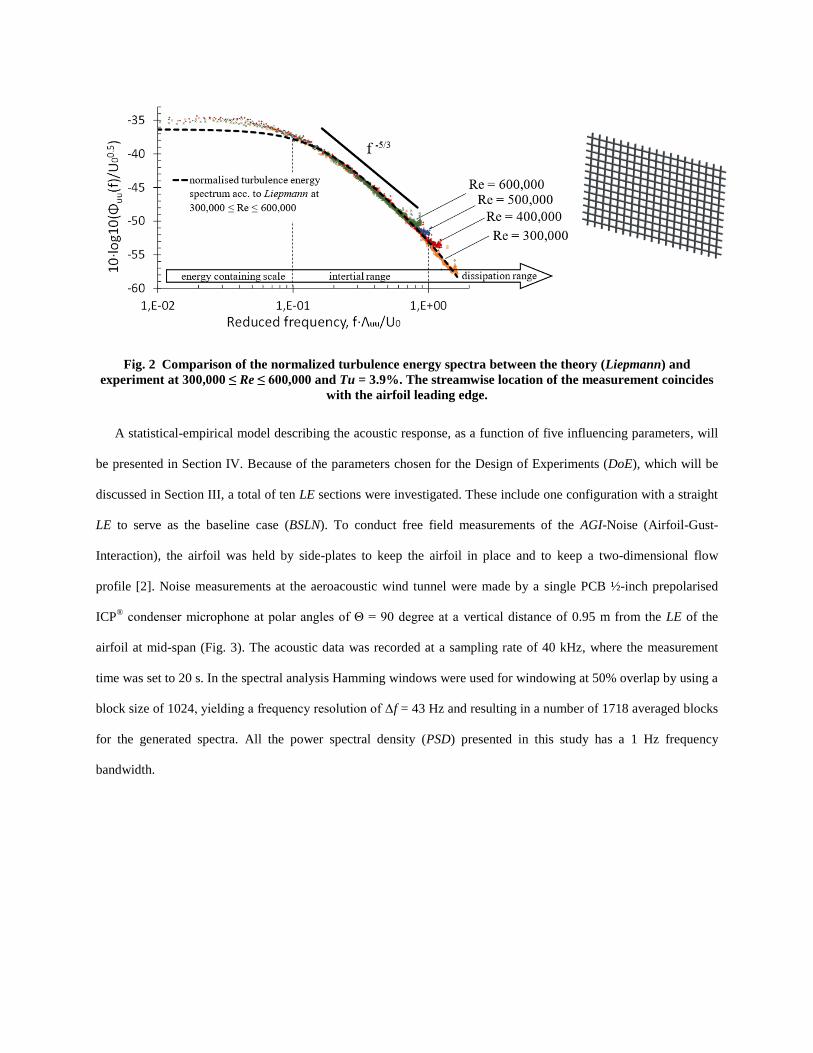
Fig. 2 Comparison of the normalized turbulence energy spectra between the theory (Liepmann) and

experiment at 300,000 ≤ Re ≤ 600,000 and Tu = 3.9%. The streamwise location of the measurement coincides

with the airfoil leading edge.

A statistical-empirical model describing the acoustic response, as a function of five influencing parameters, will

be presented in Section IV. Because of the parameters chosen for the Design of Experiments (DoE), which will be

discussed in Section III, a total of ten LE sections were investigated. These include one configuration with a straight

LE to serve as the baseline case (BSLN). To conduct free field measurements of the AGI-Noise (Airfoil-Gust-

Interaction), the airfoil was held by side-plates to keep the airfoil in place and to keep a two-dimensional flow

profile [2]. Noise measurements at the aeroacoustic wind tunnel were made by a single PCB ½-inch prepolarised

ICP® condenser microphone at polar angles of Θ = 90 degree at a vertical distance of 0.95 m from the LE of the

airfoil at mid-span (Fig. 3). The acoustic data was recorded at a sampling rate of 40 kHz, where the measurement

time was set to 20 s. In the spectral analysis Hamming windows were used for windowing at 50% overlap by using a

block size of 1024, yielding a frequency resolution of Δf = 43 Hz and resulting in a number of 1718 averaged blocks

for the generated spectra. All the power spectral density (PSD) presented in this study has a 1 Hz frequency

bandwidth.

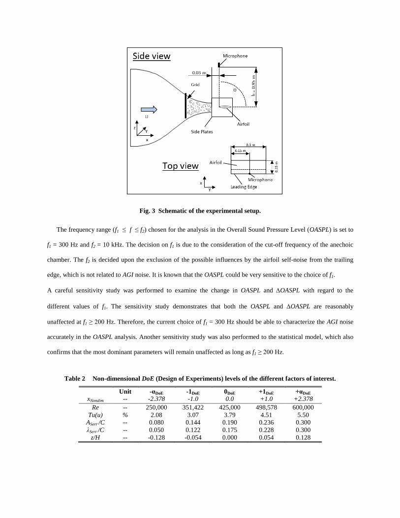
Fig. 3 Schematic of the experimental setup.

The frequency range (f1 ≤ f ≤ f2) chosen for the analysis in the Overall Sound Pressure Level (OASPL) is set to

f1 = 300 Hz and f2 = 10 kHz. The decision on f1 is due to the consideration of the cut-off frequency of the anechoic

chamber. The f2 is decided upon the exclusion of the possible influences by the airfoil self-noise from the trailing

edge, which is not related to AGI noise. It is known that the OASPL could be very sensitive to the choice of f1.

A careful sensitivity study was performed to examine the change in OASPL and OASPL with regard to the

different values of f1. The sensitivity study demonstrates that both the OASPL and OASPL are reasonably

unaffected at f1 ≥ 200 Hz. Therefore, the current choice of f1 = 300 Hz should be able to characterize the AGI noise

accurately in the OASPL analysis. Another sensitivity study was also performed to the statistical model, which also

confirms that the most dominant parameters will remain unaffected as long as f1 ≥ 200 Hz.

Table 2 Non-dimensional DoE (Design of Experiments) levels of the different factors of interest.

Unit -αDoE -1DoE 0DoE +1DoE +αDoE

xNondim -- -2.378 -1.0 0.0 +1.0 +2.378

Re -- 250,000 351,422 425,000 498,578 600,000

Tu(u) % 2.08 3.07 3.79 4.51 5.50

ASerr /C -- 0.080 0.144 0.190 0.236 0.300

λSerr /C -- 0.050 0.122 0.175 0.228 0.300

z/H -- -0.128 -0.054 0.000 0.054 0.128

A. Measurement Environment

The range of jet speeds under investigation is 25 ms-1

Uo 60 ms-1

, corresponding to Reynolds’ numbers based

on the airfoil chord length of 2x5∙105

≤ Re ≤ 6x105, respectively. As shown in Table 2, the minima and maxima

correspond to each of the five influencing parameters are defined. Preliminary measurements were performed at the

extreme flow conditions prior to the main acoustic study to ensure that the background noise of the wind tunnel

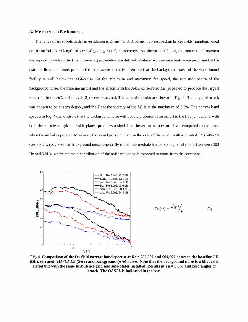
facility is well below the AGI-Noise. At the minimum and maximum fan speed, the acoustic spectra of the

background noise, the baseline airfoil and the airfoil with the A45λ7.5 serrated LE (expected to produce the largest

reduction in the AGI-noise level [2]) were measured. The acoustic results are shown in Fig. 4. The angle of attack

was chosen to be at zero degree, and the Tu at the vicinity of the LE is at the maximum of 5.5%. The narrow band

spectra in Fig. 4 demonstrate that the background noise without the presence of an airfoil in the free jet, but still with

both the turbulence grid and side-plates, produces a significant lower sound pressure level compared to the cases

when the airfoil is present. Moreover, the sound pressure level in the case of the airfoil with a serrated LE (A45λ7.5

case) is always above the background noise, especially in the intermediate frequency region of interest between 300

Hz and 5 kHz, where the main contribution of the noise reduction is expected to come from the serrations.

Fig. 4 Comparison of the far field narrow band spectra at Re = 250,000 and 600,000 between the baseline LE

(BL), serrated A45λ7.5 LE (Serr) and background (w/o) noises. Note that the background noise is without the

airfoil but with the same turbulence grid and side-plates installed. Results at Tu = 5.5% and zero angles of

attack. The OASPL is indicated in the box.

103

104

0

10

20

30

40

50

60

70

80

f, Hz

SP

L,

dB

/Hz

BL, Re 2.5e5, 71.7 dB

Serr, Re 2.5e5, 63.2 dB

w/o, Re 2.5e5, 54.1 dB

BL, Re 6.0e5, 93.6 dB

Serr, Re 6.0e5, 88.1 dB

w/o, Re 6.0e5, 74.4 dB

(3)

B. Amiet’s Flat Plate Comparison

Figure 5 shows the non-dimensionalized far-field sound pressure level spectra for both the baseline and serrated

cases. The SPL is scaled with the 4th

power of the freestream velocity Uo, while the frequency is scaled with the

airfoil semi-span and the Uo. The collapse of the spectra demonstrates that the AGI-noise can be accurately scaled

with Uo4 especially for the baseline LE case. A slight deviation can be observed for the serrated LE case, but

generally the scaling law can still be applied in this case. This particular velocity dependency is consistent with the

Amiet flat plate model [21].

Fig. 5 Non-dimensionalized SPL spectra for the baseline and serrated LE at different flow velocities. The

airfoil is set at z/H = 0 with Tu = 3.79 %. Note that the SPL for the serrated LE is shifted by 30 dB.

The Amiet model [21] was also used to validate the AGI noise produced by a baseline, straight LE airfoil in the

current setting. The Amiet’s model was modified slightly by taking into account of the consideration of the airfoil

thickness according to Gershfeld [22]:

(4)

where Λuu is the longitudinal integral length scale of the turbulence, Tu is the turbulence intensity, R is the observer

distance, b the airfoil semi-span, d is the airfoil thickness and is the normalized longitudinal wavenumber. The

Λuu and Tu were measured independently. The model takes into account of the cross-power spectral density of the

surface pressure on the airfoil caused by the turbulence.

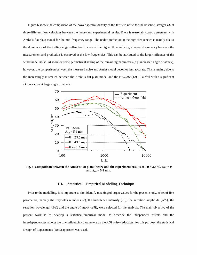
Figure 6 shows the comparison of the power spectral density of the far field noise for the baseline, straight LE at

three different flow velocities between the theory and experimental results. There is reasonably good agreement with

Amiet’s flat plate model for the mid-frequency range. The under-prediction at the high frequencies is mainly due to

the dominance of the trailing edge self-noise. In case of the higher flow velocity, a larger discrepancy between the

measurement and prediction is observed at the low frequencies. This can be attributed to the larger influence of the

wind tunnel noise. At more extreme geometrical setting of the remaining parameters (e.g. increased angle of attack),

however, the comparison between the measured noise and Amiet model becomes less accurate. This is mainly due to

the increasingly mismatch between the Amiet’s flat plate model and the NACA65(12)-10 airfoil with a significant

LE curvature at large angle of attack.

Fig. 6 Comparison between the Amiet’s flat plate theory and the experiment results at Tu = 3.8 %, z/H = 0

and Λuu = 5.8 mm.

III. Statistical – Empirical Modelling Technique

Prior to the modelling, it is important to first identify meaningful target values for the present study. A set of five

parameters, namely the Reynolds number (Re), the turbulence intensity (Tu), the serration amplitude (A/C), the

serration wavelength (λ/C) and the angle of attack (z/H), were selected for the analysis. The main objective of the

present work is to develop a statistical-empirical model to describe the independent effects and the

interdependencies among the five influencing parameters on the AGI noise-reduction. For this purpose, the statistical

Design of Experiments (DoE) approach was used.

When analyzing a defined physical experimental space by varying several influencing parameters, the classical

method would be to vary one of the parameters, while the others remain constant. This procedure will then be

repeated for each parameter of interest (raster method). This might be an easy and effective method to describe the

influence of these parameters on a certain response variable with a high accuracy, as long as the number of

parameters is small, and the interdependencies between the parameters are disregarded.

An increase of the parameters inevitably leads to an exponential rise of the necessary measurement trials (MT).

According to the n-permutation in Eq. (5), analyzing a system with five parameters (k) and varying the parameters

on five levels each (n) will result in 3125 trials. This represents a hardly manageable experimental volume. Instead,

applying the statistical Design of Experiments (DoE) approach as per the Eq. 6 could lead to a significant reduction

of the experimental volume to 43 trials without a significant loss of information on the system behavior. This

approach keeps the experimental volume manageable and facilitates the detailed analysis of multiple parameters

with a reasonably high accuracy.

(5)

(6)

A. Design of Experiments (DoE) Methodology

The objective of the experimental modelling is the ability to describe the defined experimental space by means

of functions that take into account of all the influencing parameters of significance (Eq. 7). For this purpose, the

response variables (RV) have to be defined in order to act as target values of the regression functions. The

coefficients are determined in accordance to the chosen set of influencing parameters (IP).

(7)

The Design of Experiments methodology is based on the definition of an experimental space for a setup that

consists a full factorial core [-1 ... +1], star points [-α ... +α] that label the upper and lower experimental boundaries,

and a central point [0], which is defined as the experimental adjustment where all the parameters are on their

intermediary values [23–26]. Based on this experimental composition of the DoE methodology, the analytical

statistic gathers the population from a subset. A circumscribed central composite design (CCD) was chosen as the

appropriate experimental design. Circumscribed CCDs are characterized by statistical properties, such as the

orthogonality or rotatability [27].

An experimental design is defined as rotatable, if the variance of the probability distribution is a function of the

distance between the star point and the central point, and not of the direction, as is the case with orthogonality.

Given a set of points within the experimental space at a constant distance to the central point, the rotatable design

shows a consistent accuracy in the prediction for all the points. With regards to the statistical analysis, this property

is highly advantageous [23]. On the contrary, the orthogonal designs are advantageous because they can avoid the

confounding of the effects. This enables the determination of all the regression coefficients independently [28, 29].

In general, the α-values (star point locations) are higher than the coordinates of the central core (αDoE > 1), thus

represent the limits of the experimental space. Consequently, each factor is varied as a combination of the five non-

dimensional levels [+α, +1, 0, -1, -α]. A special design is the combination of both the properties in orthogonality and

rotatability. As the requirements of orthogonality are not completely grantable while simultaneously guaranteeing

the rotatability, this design is defined as pseudo-orthogonal and rotatable. It combines the advantages of both

properties, especially because the resulting confounding is of negligible magnitude (< 0.02%).

As already described, the Design of Experiments approach is limited to describing the experimental space of

interest by the functions of first and second order as well as linear interdependencies between the single influencing

parameters (Eq. 7). In order to choose a valid model, preliminary investigations are necessary to ensure that the

system satisfies these conditions. With this purpose all the five influencing parameters were analyzed individually in

a preliminary study and their effects on the target values were evaluated carefully. This analysis, in combination

with the defined experimental design, results in the test matrix as shown in Table 2, which also includes the upper

and lower parameter settings. The total number of measurement point is 43, in addition to 16 repetitions for the

central point in order to define a system-characteristic statistical spread, and to guarantee the desired statistical

features. The trials of the strategically planned experiment were performed in a random order and they were

repeated twice to obtain the average values. This procedure is to secure the reduction and elimination of unknown

and uncontrollable quantities. Additionally, the analysis of the statistical significance allows the elimination of

parameters with impacts on the response variable that is smaller than the statistical spread.

B. Response Variables

The response variables (RV) can be described by means of all influencing parameters in the first and second

order as well as the interdependencies between the influencing parameters (Eq. 7). Defining the response variables is

a crucial part of evaluating the experimental data. They are expected to describe the system with the necessary

accuracy. This study focuses on the overall sound reduction of serrated LE compared to a baseline LE, and does not

predict the SPL at a particular frequency. Consequently, the response variables of interest are limited to the OASPL.

To define a sound pressure reduction level, information on both the baseline and the serrated LE are necessary. It is

important to note that single microphone measurements were performed, hence, information on the sound

directivity, overall sound power levels and sound power reduction are not available.

However, the dependencies of the sound generation itself are also of interest because it facilitates the analysis of

the influence of each case on the reduction independently. As shown in Eq. (8), the noise produced by a baseline LE

is a function of the Reynolds number, turbulence intensity and angle of attack. In the case of serrated LE, additional

influences of the serration wavelength and amplitude must be taken into consideration (Eq. 9).

(8)

(9)

Note that pref = 2x10-5

Pa and the frequency range of interest is between 300 Hz and 10 kHz. Subtracting the

OASPLSerr from the OASPLBL gives the overall sound pressure level reduction ΔOASPL (Eq. 10).

(10)

IV. Selection of Key Noise Results

Generally, as shown in Fig. 7a, the serration amplitude is the main factor in reducing the broadband noise. At Re

= 425,000, Tu = 3.79% and z/H = 0, the LE serration is found to be the most effective in frequency range between

850 Hz and 3500 Hz, where an average sound pressure level reduction of up to ΔSPL ≈ 10 dB is achieved by the

largest serration amplitude (A/C = 0.3).

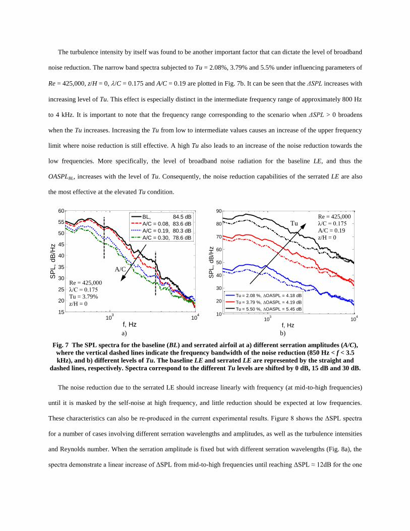
The turbulence intensity by itself was found to be another important factor that can dictate the level of broadband

noise reduction. The narrow band spectra subjected to Tu = 2.08%, 3.79% and 5.5% under influencing parameters of

Re = 425,000, z/H = 0, /C = 0.175 and A/C = 0.19 are plotted in Fig. 7b. It can be seen that the ΔSPL increases with

increasing level of Tu. This effect is especially distinct in the intermediate frequency range of approximately 800 Hz

to 4 kHz. It is important to note that the frequency range corresponding to the scenario when ΔSPL > 0 broadens

when the Tu increases. Increasing the Tu from low to intermediate values causes an increase of the upper frequency

limit where noise reduction is still effective. A high Tu also leads to an increase of the noise reduction towards the

low frequencies. More specifically, the level of broadband noise radiation for the baseline LE, and thus the

OASPLBL, increases with the level of Tu. Consequently, the noise reduction capabilities of the serrated LE are also

the most effective at the elevated Tu condition.

a) b)

Fig. 7 The SPL spectra for the baseline (BL) and serrated airfoil at a) different serration amplitudes (A/C),

where the vertical dashed lines indicate the frequency bandwidth of the noise reduction (850 Hz < f < 3.5

kHz), and b) different levels of Tu. The baseline LE and serrated LE are represented by the straight and

dashed lines, respectively. Spectra correspond to the different Tu levels are shifted by 0 dB, 15 dB and 30 dB.

The noise reduction due to the serrated LE should increase linearly with frequency (at mid-to-high frequencies)

until it is masked by the self-noise at high frequency, and little reduction should be expected at low frequencies.

These characteristics can also be re-produced in the current experimental results. Figure 8 shows the ΔSPL spectra

for a number of cases involving different serration wavelengths and amplitudes, as well as the turbulence intensities

and Reynolds number. When the serration amplitude is fixed but with different serration wavelengths (Fig. 8a), the

spectra demonstrate a linear increase of ΔSPL from mid-to-high frequencies until reaching ΔSPL ≈ 12dB for the one

103

104

15

20

25

30

35

40

45

50

55

60

f, Hz

SP

L,

dB

/Hz

BL, 84.5 dB

A/C = 0.08, 83.6 dB

A/C = 0.19, 80.3 dB

A/C = 0.30, 78.6 dB

103

104

10

20

30

40

50

60

70

80

90

f, Hz

SP

L,

dB

/Hz

Tu = 2.08 %, OASPL = 4.18 dB

Tu = 3.79 %, OASPL = 4.19 dB

Tu = 5.50 %, OASPL = 5.45 dB

A/C

Re = 425,000

λ/C = 0.175

Tu = 3.79%

z/H = 0

Tu Re = 425,000

λ/C = 0.175

A/C = 0.19

z/H = 0

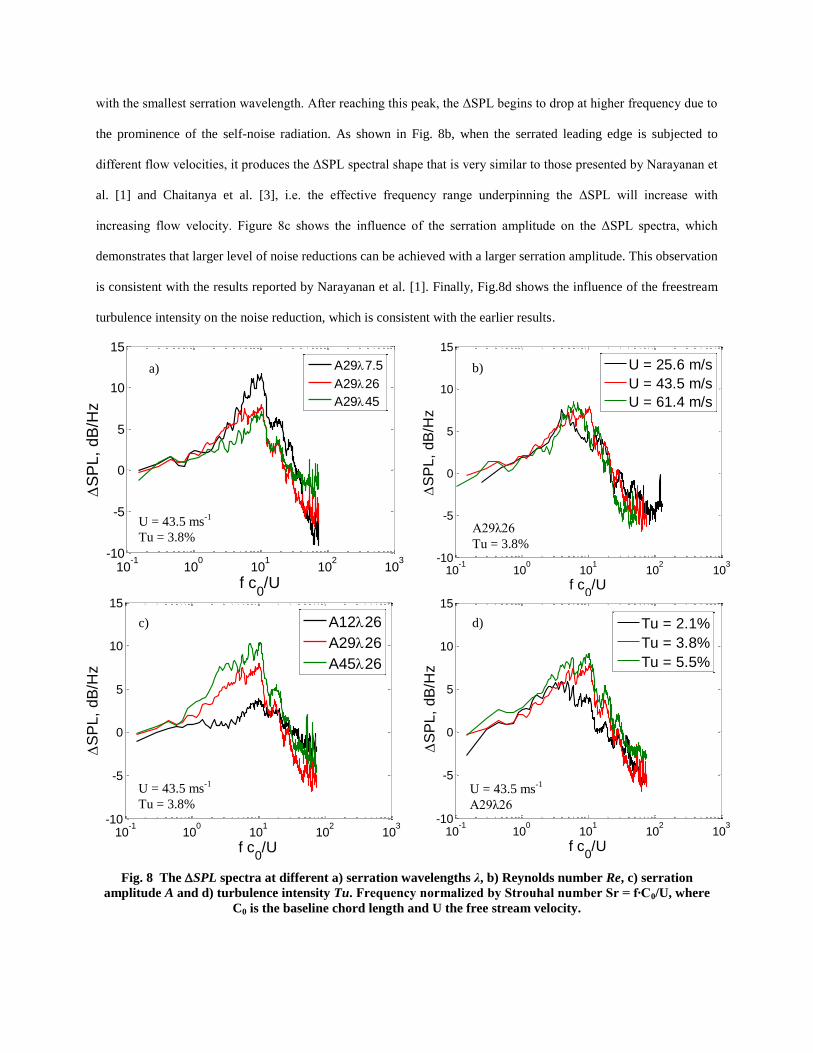
with the smallest serration wavelength. After reaching this peak, the ΔSPL begins to drop at higher frequency due to

the prominence of the self-noise radiation. As shown in Fig. 8b, when the serrated leading edge is subjected to

different flow velocities, it produces the ΔSPL spectral shape that is very similar to those presented by Narayanan et

al. [1] and Chaitanya et al. [3], i.e. the effective frequency range underpinning the ΔSPL will increase with

increasing flow velocity. Figure 8c shows the influence of the serration amplitude on the ΔSPL spectra, which

demonstrates that larger level of noise reductions can be achieved with a larger serration amplitude. This observation

is consistent with the results reported by Narayanan et al. [1]. Finally, Fig.8d shows the influence of the freestream

turbulence intensity on the noise reduction, which is consistent with the earlier results.

Fig. 8 The SPL spectra at different a) serration wavelengths λ, b) Reynolds number Re, c) serration

amplitude A and d) turbulence intensity Tu. Frequency normalized by Strouhal number Sr = f∙C0/U, where

C0 is the baseline chord length and U the free stream velocity.

10-1

100

101

102

103

-10

-5

0

5

10

15

f c0/U

S

PL

, d

B/H

z

A297.5

A2926

A2945

10-1

100

101

102

103

-10

-5

0

5

10

15

f c0/U

S

PL,

dB

/Hz

U = 25.6 m/s

U = 43.5 m/s

U = 61.4 m/s

10-1

100

101

102

103

-10

-5

0

5

10

15

f c0/U

S

PL

, d

B/H

z

A1226

A2926

A4526

10-1

100

101

102

103

-10

-5

0

5

10

15

f c0/U

S

PL,

dB

/Hz

Tu = 2.1%

Tu = 3.8%

Tu = 5.5%

A29λ26

Tu = 3.8%

U = 43.5 ms-1

Tu = 3.8%

U = 43.5 ms-1

A29λ26

U = 43.5 ms-1

Tu = 3.8%

a) b)

c) d)

A. General System Information

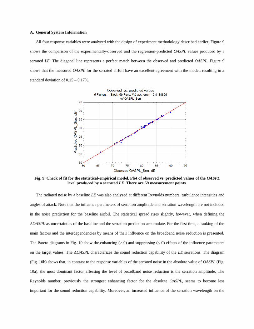
All four response variables were analyzed with the design of experiment methodology described earlier. Figure 9

shows the comparison of the experimentally-observed and the regression-predicted OASPL values produced by a

serrated LE. The diagonal line represents a perfect match between the observed and predicted OASPL. Figure 9

shows that the measured OASPL for the serrated airfoil have an excellent agreement with the model, resulting in a

standard deviation of 0.15 – 0.17%.

Fig. 9 Check of fit for the statistical-empirical model. Plot of observed vs. predicted values of the OASPL

level produced by a serrated LE. There are 59 measurement points.

The radiated noise by a baseline LE was also analyzed at different Reynolds numbers, turbulence intensities and

angles of attack. Note that the influence parameters of serration amplitude and serration wavelength are not included

in the noise prediction for the baseline airfoil. The statistical spread rises slightly, however, when defining the

ΔOASPL as uncertainties of the baseline and the serration prediction accumulate. For the first time, a ranking of the

main factors and the interdependencies by means of their influence on the broadband noise reduction is presented.

The Pareto diagrams in Fig. 10 show the enhancing (> 0) and suppressing (< 0) effects of the influence parameters

on the target values. The ΔOASPL characterizes the sound reduction capability of the LE serrations. The diagram

(Fig. 10b) shows that, in contrast to the response variables of the serrated noise in the absolute value of OASPL (Fig.

10a), the most dominant factor affecting the level of broadband noise reduction is the serration amplitude. The

Reynolds number, previously the strongest enhancing factor for the absolute OASPL, seems to become less

important for the sound reduction capability. Moreover, an increased influence of the serration wavelength on the

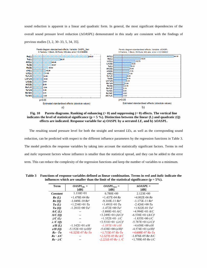
sound reduction is apparent in a linear and quadratic form. In general, the most significant dependencies of the

overall sound pressure level reduction (ΔOASPL) demonstrated in this study are consistent with the findings of

previous studies [3, 2, 30–33, 5, 34, 35].

a) b)

Fig. 10 Pareto diagrams. Ranking of enhancing (> 0) and suppressing (< 0) effects. The vertical line

indicates the level of statistical significance (p = 5 %). Distinction between the linear (L) and quadratic (Q)

effects are indicated. Response variable for a) OASPL by a serrated LE, and b) ΔOASPL.

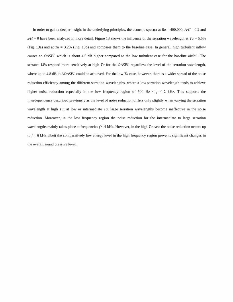
The resulting sound pressure level for both the straight and serrated LEs, as well as the corresponding sound

reduction, can be predicted with respect to the different influence parameters by the regression functions in Table 3.

The model predicts the response variables by taking into account the statistically significant factors. Terms in red

and italic represent factors whose influence is smaller than the statistical spread, and they can be added to the error

term. This can reduce the complexity of the regression functions and keep the number of variables to a minimum.

Table 3 Functions of response variables defined as linear combination. Terms in red and italic indicate the

influences which are smaller than the limit of the statistical significance (p = 5%).

Term OASPLBL = OASPLSerr = ΔOASPL =

[dB] [dB] [dB]

Constant 1.116E+01 6.780E+00 2.123E+00

Re (L) +1.478E-04∙Re +1.437E-04∙Re +4.002E-06∙Re

Re (Q) -1.049E-10∙Re² -9.310E-11∙Re² -1.175E-11∙Re²

Tu (L) +1.234E+01∙Tu +1.491E+01∙Tu -2.426E+00∙Tu

Tu (Q) -1.281E+00∙Tu² -1.472E+00∙Tu² +1.922E-01∙Tu²

A/C (L) -- -3.800E+01∙A/C +4.994E+01∙A/C

A/C (Q) -- +3.249E+01∙(A/C)² -6.538E+01∙(A/C)²

λ/C (L) -- +1.352E+01∙ λ/C -1.835E+00∙λ/C

λ /C (Q) -- +3.531E+01∙ (λ/C)² -5.787E+01∙(λ/C)²

z/H (L) -1.142E+01∙z/H -1.357E+01∙z/H +4.658E+00∙z/H

z/H (Q) -5.152E+01∙(z/H)² -5.638E+00∙(z/H)² -4.574E+01∙(z/H)²

Re ∙ Tu +6.323E-07∙Re∙Tu +1.715E-07∙Re∙Tu +4.608E-07∙Re∙Tu

Re ∙ A/C -- +2.327E-05∙Re∙A/C -1.876E-05∙Re∙A/C

Re ∙ λ/C -- -2.221E-05∙Re∙ λ /C +1.709E-05∙Re∙λ/C

Re ∙ z/H -8.150E-06∙Re∙z/H +1.574E-05∙Re∙z/H -2.389E-05∙Re∙z/H

Tu ∙ A/C -- -2.349E+00∙Tu∙A/C +1.951E+00∙Tu∙A/C

Tu ∙ λ/C -- -4.268E+00∙Tu∙ λ/C +3.847E+00∙Tu∙λ/C

Tu ∙ z/H +3.069E+00∙Tu∙z/H +2.115E+00∙Tu∙z/H +9.546E-01∙Tu∙z/H

A/C ∙ λ/C -- +2.290E+01∙A/C∙ λ /C -2.521E+01∙A/C∙λ/C

A/C ∙ z/H -- +6.987E+00∙A/C∙z/H -1.649E+01∙A/C∙z/H

λ/C ∙ z/H -- -4.926E+01∙ λ/C∙z/H 4.524E+01∙λ/C∙z/H

The intermediate effect on the influencing parameters within the experimental space on the overall noise

reduction is plotted in Fig 11. The serration amplitude has the highest intermediate effect with an almost linear

relationship between the A/C and ΔOASPL, before reaching an asymptotic level when the A/C is increased further.

The serration wavelength /C shows a non-linear behavior where the optimum is achieved at intermediate

wavelength, beyond which the noise reduction capability is weakened considerably. The predicted profile for the

influence of the turbulence intensity Tu exhibits a large level of noise reduction at high Tu levels. On the contrary, at

a band of low Tu, low level of noise reduction is predicted. This is in agreement with the measurements shown in

Fig. 7b, where a high Tu is identified to be able to cause a high level of broadband noise radiation from a baseline

airfoil. This in turn facilitates an increase of the noise reduction capability when a serrated LE is used. However, it is

important to note that the effects of the individual parameters on the overall noise reduction in Fig. 11 cannot be

attributed to the serrated LEs only. This is because different levels of Re, Tu and angle of attack (z/H) can also affect

the baseline straight LE. Thus, a more detailed analysis of the noise reduction by the serration requires an

independent analysis of the noise radiation by the baseline and serrated airfoil, respectively.

Fig. 11 Intermediate impact of the influencing parameters on the ΔOASPL, including the error band. The

horizontal blue band indicates average noise reduction by the use of serrated LEs.

B. Interdependency of serration wavelength and turbulence intensity (λ/C ∙ Tu)

A significant effect identifiable in the response variable ΔOASPL was found to be an interdependency of the

serration wavelength and the turbulence intensity (λ/C·Tu), as can be seen in the Pareto diagram (Fig. 10b). At low

Tu, small serration wavelengths are needed in order to achieve a high level of noise reduction, as exhibited by the

red color region in Fig. 12. As the Tu is related to the integral length scale Λuu of the incoming gust, large serration

wavelengths are expected to be less effective in the de-correlation effects especially if the incoming gust is

characterized by small turbulent eddies. Previous investigations suggested that serration wavelengths should be

small to achieve good level of noise reduction, although in general the impact of the serration wavelength is not as

dominant as the serration amplitude [3, 5, 2]. The interdependency in Fig. 12 shows that the optimum serration

wavelength highly depends on the incoming Tu level. Low to intermediate Tu support the previous findings that a

smaller serration wavelength is more desirable. However, at high Tu, serration wavelengths of intermediate values

are far more effective in reducing the OASPL, as shown in Fig 12. This agrees with the finding of a recent work [3],

where the optimum serration wavelength is found to be twice the size of the incoming turbulent structure in the form

of the integral length scale Λuu. An optimal set of Tu and λ/C leads to a reduction of the fluctuating acoustic pressure

of about 53% to that produced by the baseline airfoil.

Fig. 12 Influence of interdependency between the serration wavelength (λ/C) and turbulence intensity (Tu)

on the ΔOASPL. Other influencing factors remain on intermediate levels (Re = 425,000, A/C = 0.19, z/H = 0).

In order to gain a deeper insight in the underlying principles, the acoustic spectra at Re = 400,000, A/C = 0.2 and

z/H = 0 have been analyzed in more detail. Figure 13 shows the influence of the serration wavelength at Tu = 5.5%

(Fig. 13a) and at Tu = 3.2% (Fig. 13b) and compares them to the baseline case. In general, high turbulent inflow

causes an OASPL which is about 4.5 dB higher compared to the low turbulent case for the baseline airfoil. The

serrated LEs respond more sensitively at high Tu for the OASPL regardless the level of the serration wavelength,

where up to 4.8 dB in OASPL could be achieved. For the low Tu case, however, there is a wider spread of the noise

reduction efficiency among the different serration wavelengths, where a low serration wavelength tends to achieve

higher noise reduction especially in the low frequency region of 300 Hz ≤ f ≤ 2 kHz. This supports the

interdependency described previously as the level of noise reduction differs only slightly when varying the serration

wavelength at high Tu; at low or intermediate Tu, large serration wavelengths become ineffective in the noise

reduction. Moreover, in the low frequency region the noise reduction for the intermediate to large serration

wavelengths mainly takes place at frequencies f ≤ 4 kHz. However, in the high Tu case the noise reduction occurs up

to f = 6 kHz albeit the comparatively low energy level in the high frequency region prevents significant changes in

the overall sound pressure level.

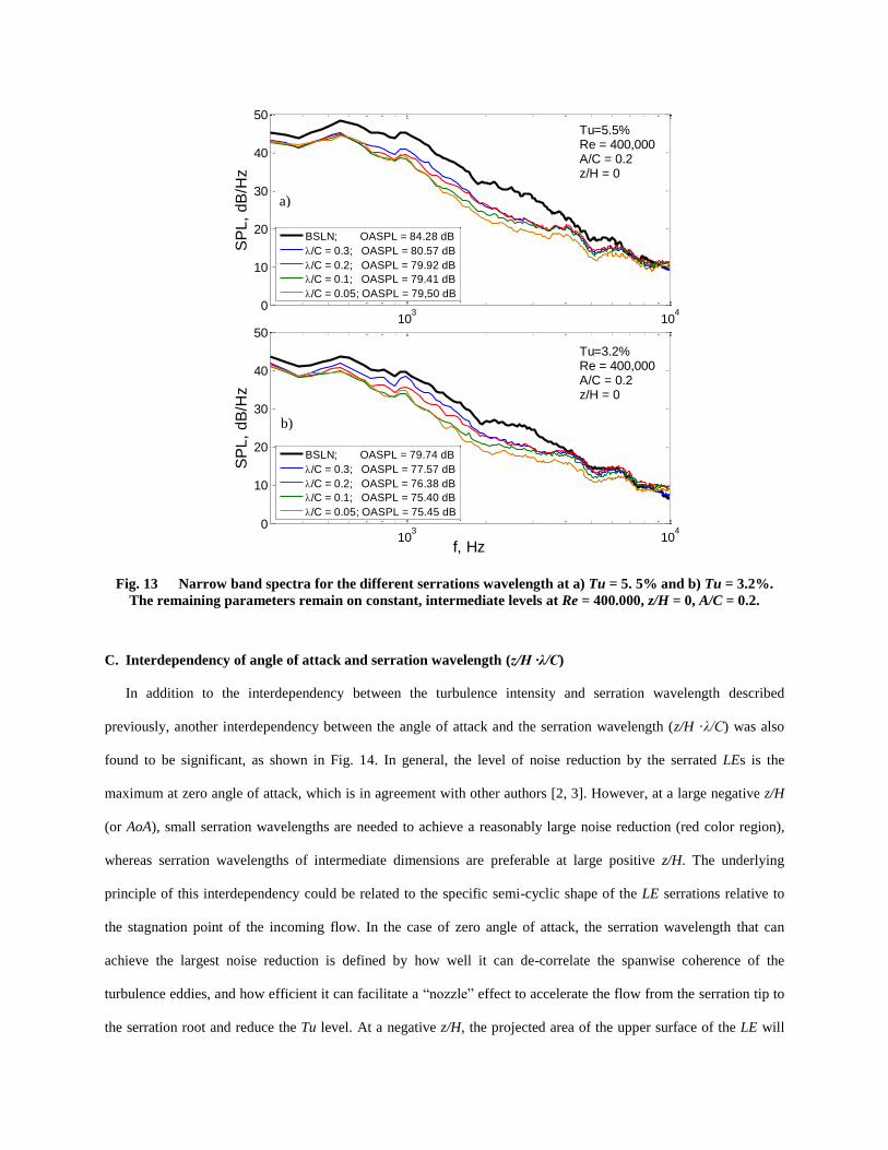
Fig. 13 Narrow band spectra for the different serrations wavelength at a) Tu = 5. 5% and b) Tu = 3.2%.

The remaining parameters remain on constant, intermediate levels at Re = 400.000, z/H = 0, A/C = 0.2.

C. Interdependency of angle of attack and serration wavelength (z/H ∙λ/C)

In addition to the interdependency between the turbulence intensity and serration wavelength described

previously, another interdependency between the angle of attack and the serration wavelength (z/H ·λ/C) was also

found to be significant, as shown in Fig. 14. In general, the level of noise reduction by the serrated LEs is the

maximum at zero angle of attack, which is in agreement with other authors [2, 3]. However, at a large negative z/H

(or AoA), small serration wavelengths are needed to achieve a reasonably large noise reduction (red color region),

whereas serration wavelengths of intermediate dimensions are preferable at large positive z/H. The underlying

principle of this interdependency could be related to the specific semi-cyclic shape of the LE serrations relative to

the stagnation point of the incoming flow. In the case of zero angle of attack, the serration wavelength that can

achieve the largest noise reduction is defined by how well it can de-correlate the spanwise coherence of the

turbulence eddies, and how efficient it can facilitate a “nozzle” effect to accelerate the flow from the serration tip to

the serration root and reduce the Tu level. At a negative z/H, the projected area of the upper surface of the LE will

103

104

0

10

20

30

40

50

Tu=5.5% Re = 400,000A/C = 0.2 z/H = 0

SP

L,

dB

/Hz

103

104

0

10

20

30

40

50

Tu=3.2% Re = 400,000A/C = 0.2 z/H = 0

f, Hz

SP

L,

dB

/Hz

BSLN; OASPL = 79.74 dB

/C = 0.3; OASPL = 77.57 dB

/C = 0.2; OASPL = 76.38 dB

/C = 0.1; OASPL = 75.40 dB

/C = 0.05; OASPL = 75.45 dB

BSLN; OASPL = 84.28 dB

/C = 0.3; OASPL = 80.57 dB

/C = 0.2; OASPL = 79.92 dB

/C = 0.1; OASPL = 79.41 dB

/C = 0.05; OASPL = 79,50 dB

a)

b)

cause a significant impingement upon the incoming gusts. In this case, the use of small wavelength serrations is a

logical choice.

Fig. 14 Influence of interdependency between the serration wavelength and angle of attack (λ/C · z/H) on

the ΔOASPL. Other influencing factors remain on the intermediate levels (Re = 425,000, A/C = 0.19, Tu =

3.8%).

This is because a small serration wavelength will cause many three-dimensional undulations on the upper surface

of the LE, which will maintain the serration effect to achieve the interaction noise reduction.

In the case of a positive z/H, the incoming flow will naturally impinge on the lower surface of the LE. However, the

planar geometry at the lower surface of the serrated LE means that the three-dimensional undulation can no longer

be achieved by using a small serration wavelength. Instead, a larger serration wavelength is preferable to avoid the

direct impingement between the incoming gusts and the LE geometry.

Of particular interest is the impact of this interdependency (z/H ·λ/C) on the narrow band spectral characteristic.

It has already been known that the smallest serration wavelength does not necessarily lead to a maximum noise

reduction across the whole frequency range [2]. A first indicator for the effect of small serration wavelengths on the

noise can be found in the high frequency region above 10 kHz (Fig. 15), where all the different serration

wavelengths actually lead to noise increase. It is clear that the largest noise increase occurs at the smallest serration

wavelengths. However, this effect is neglected in the present study because the lower and upper frequency limits for

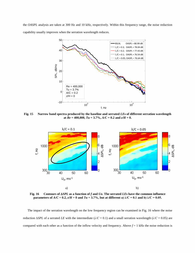
the OASPL analysis are taken at 300 Hz and 10 kHz, respectively. Within this frequency range, the noise reduction

capability usually improves when the serration wavelength reduces.

Fig. 15 Narrow band spectra produced by the baseline and serrated LEs of different serration wavelength

at Re = 400,000, Tu = 3.7%, A/C = 0.2 and z/H = 0.

a) b)

Fig. 16 Contours of SPL as a function of f and Uo. The serrated LEs have the common influence

parameters of A/C = 0.2, z/H = 0 and Tu = 3.7%, but at different a) λ/C = 0.1 and b) λ/C = 0.05.

The impact of the serration wavelength on the low frequency region can be examined in Fig. 16 where the noise

reduction SPL of a serrated LE with the intermediate (λ/C = 0.1) and a small serration wavelength (λ/C = 0.05) are

compared with each other as a function of the inflow velocity and frequency. Above f = 1 kHz the noise reduction is

103

104

-10

0

10

20

30

40

50

f, Hz

SP

L,

dB

/Hz

BSLN; OASPL = 80.99 dB

/C = 0.3; OASPL = 78.04 dB

/C = 0.2; OASPL = 77.43 dB

/C = 0.1; OASPL = 76.54 dB

/C = 0.05; OASPL = 76.64 dB

Re = 400,000

Tu = 3.7%

A/C = 0.2

z/H = 0

significantly higher for the small serration wavelength (Fig. 16b). However, as indicated by the circled black region

in Fig. 16a, the level of noise reduction is higher for the intermediate wavelength in a frequency range of 500 Hz f

1.2 kHz. As a result, the ΔOASPL is slightly higher for the intermediate λ/C = 0.1 case.

Figure 17 shows the SPL spectra produced by the baseline and serrated LEs of a slightly larger serration

wavelength (λ/C = 0.175) at different angles of attack AoA (or z/H). At first glance, it is clear that the largest level of

noise reduction occurs at z/H > 0 and across the widest frequency range (Fig. 17a). The level and frequency range of

the noise reduction are lessened as the z/H decreases. However, a closer examination shows that the sensitivities of

the SPL and OASPL to the z/H are different between the baseline and serrated LEs. For the baseline LE, the lowest

OASPL is achieved at z/H < 0 what is mainly due to the low level of noise radiation in the frequency range of 2 kHz

≤ f ≤ 4 kHz. The largest level of OASPL produced by the baseline airfoil, on the other hand, is achieved at z/H = 0.

The noise level produced at z/H > 0 lies in between. For the serrated LE, the lowest level of the OASPL is achieved

at z/H > 0. As the z/H slowly decreases, the level of OASPL increases. This contradictory behavior between the

baseline and serrated LEs for the noise radiation should be taken into consideration when examining the

interdependency (z/H ·λ/C) for the SPL or OASPL.

In Fig. 17c, when the airfoil is set at z/H = –0.128, there is little noise reduction at 1.2 kHz f 3.8 kHz because

of the opposite trends in SPL produced by the baseline airfoil (reduction in the SPL level) and serrated airfoil

(increase in the SPL level), respectively. At f > 3.8 kHz, the serrated LE even causes a significant noise increase

which is not due to the experimental error as we have re-tested it many times. Rather, the presence of the serration

wavelength actually facilitates cross-flow from the projected upper surface of the LE, through the serration air gaps

and exits the lower surface of the LE. This particular fluid–structure interaction causes the noise to increase at high

frequency that will otherwise be absence in a baseline LE. This conjecture is supported by the clear trend from other

results where the noise increase at high frequency will gradually cease to exist when the angle of attack increases.

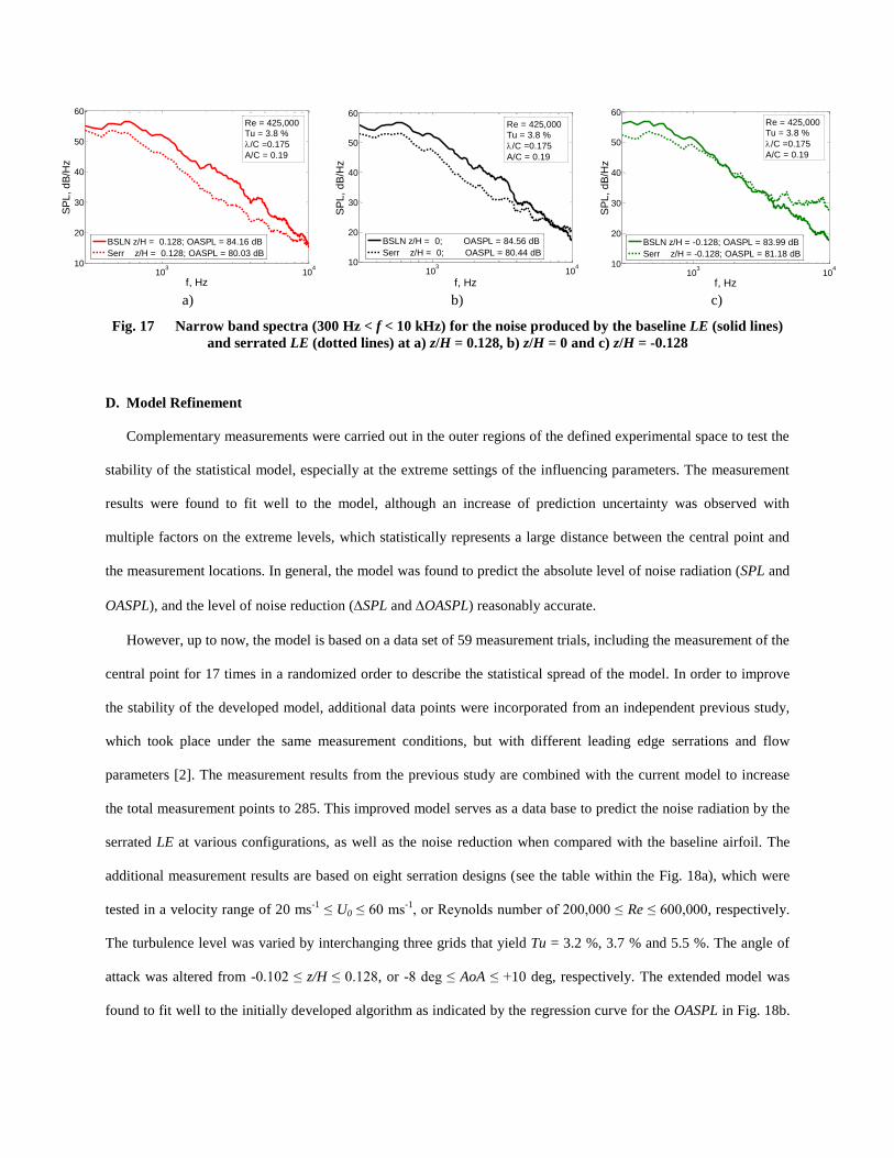
a) b) c)

Fig. 17 Narrow band spectra (300 Hz < f < 10 kHz) for the noise produced by the baseline LE (solid lines)

and serrated LE (dotted lines) at a) z/H = 0.128, b) z/H = 0 and c) z/H = -0.128

D. Model Refinement

Complementary measurements were carried out in the outer regions of the defined experimental space to test the

stability of the statistical model, especially at the extreme settings of the influencing parameters. The measurement

results were found to fit well to the model, although an increase of prediction uncertainty was observed with

multiple factors on the extreme levels, which statistically represents a large distance between the central point and

the measurement locations. In general, the model was found to predict the absolute level of noise radiation (SPL and

OASPL), and the level of noise reduction (SPL and OASPL) reasonably accurate.

However, up to now, the model is based on a data set of 59 measurement trials, including the measurement of the

central point for 17 times in a randomized order to describe the statistical spread of the model. In order to improve

the stability of the developed model, additional data points were incorporated from an independent previous study,

which took place under the same measurement conditions, but with different leading edge serrations and flow

parameters [2]. The measurement results from the previous study are combined with the current model to increase

the total measurement points to 285. This improved model serves as a data base to predict the noise radiation by the

serrated LE at various configurations, as well as the noise reduction when compared with the baseline airfoil. The

additional measurement results are based on eight serration designs (see the table within the Fig. 18a), which were

tested in a velocity range of 20 ms-1

≤ U0 ≤ 60 ms-1

, or Reynolds number of 200,000 ≤ Re ≤ 600,000, respectively.

The turbulence level was varied by interchanging three grids that yield Tu = 3.2 %, 3.7 % and 5.5 %. The angle of

attack was altered from -0.102 ≤ z/H ≤ 0.128, or -8 deg ≤ AoA ≤ +10 deg, respectively. The extended model was

found to fit well to the initially developed algorithm as indicated by the regression curve for the OASPL in Fig. 18b.

103

104

10

20

30

40

50

60

f, Hz

SP

L,

dB

/Hz

BSLN z/H = 0.128; OASPL = 84.16 dB

Serr z/H = 0.128; OASPL = 80.03 dB

Re = 425,000

Tu = 3.8 %

/C =0.175

A/C = 0.19

103

104

10

20

30

40

50

60

f, Hz

SP

L,

dB

/Hz

BSLN z/H = 0; OASPL = 84.56 dB

Serr z/H = 0; OASPL = 80.44 dB

Re = 425,000

Tu = 3.8 %

/C =0.175

A/C = 0.19

103

104

10

20

30

40

50

60

f, Hz

SP

L,

dB

/Hz

BSLN z/H = -0.128; OASPL = 83.99 dB

Serr z/H = -0.128; OASPL = 81.18 dB

Re = 425,000

Tu = 3.8 %

/C =0.175

A/C = 0.19

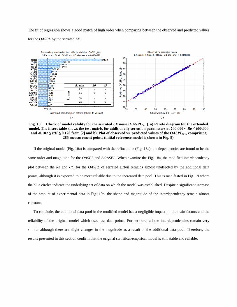
The fit of regression shows a good match of high order when comparing between the observed and predicted values

for the OASPL by the serrated LE.

a) b)

Fig. 18 Check of model validity for the serrated LE noise (OASPLSerr). a) Pareto diagram for the extended

model. The insert table shows the test matrix for additionally serration parameters at 200,000 ≤ Re ≤ 600,000

and -0.102 ≤ z/H ≤ 0.128 from [2] and b) Plot of observed vs. predicted values of the OASPLSerr comprising

285 measurement points (initial reference model is shown in Fig. 9).

If the original model (Fig. 10a) is compared with the refined one (Fig. 18a), the dependencies are found to be the

same order and magnitude for the OASPL and OASPL. When examine the Fig. 18a, the modified interdependency

plot between the Re and λ/C for the OASPL of serrated airfoil remains almost unaffected by the additional data

points, although it is expected to be more reliable due to the increased data pool. This is manifested in Fig. 19 where

the blue circles indicate the underlying set of data on which the model was established. Despite a significant increase

of the amount of experimental data in Fig. 19b, the shape and magnitude of the interdependency remain almost

constant.

To conclude, the additional data pool in the modified model has a negligible impact on the main factors and the

reliability of the original model which uses less data points. Furthermore, all the interdependencies remain very

similar although there are slight changes in the magnitude as a result of the additional data pool. Therefore, the

results presented in this section confirm that the original statistical-empirical model is still stable and reliable.

A, mm 30 45

λ ,

mm

7.5 x x

15 x x

30 x x

45 x x

a) b)

Fig. 19 Comparison of interdependency between the (Re · λ/C) for the a) original model, and b) improved

model by the use of additional data points (circles) obtained from [2].

E. Polyoptimum of noise reduction and noise radiation

The purpose of the current system is to reduce the broadband LE noise caused by the interaction between the

high turbulent inflow conditions and the LE. Therefore, in addition to the main focus on achieving high level of

noise reduction as defined by the relative difference between airfoils with straight and serrated LEs, it is also

desirable to produce low absolute magnitude of the overall sound pressure. An algorithm has been developed to

define a polyoptimum of the radiated noise and the noise reduction capability by the serrated LEs.

Of further interest is the qualitative information on the impact of the different influencing parameters on the

polyoptimum. As shown in Fig. 20 the independent response variables OASPLSerr and ΔOASPL were weighted with

an emphasis on the reduction of the OASPL. This means that the OASPL is weighted linearly between 50 – 70 dB

where 50 dB equals to an acceptability of 100%. In contrast, the ΔOASPL accounts for zero percent acceptability at

2 dB with a slope of 2 until reaching the desired optimum of 10 dB overall noise reduction (100% acceptability).

Fig. 20 Weighted functions of the single analyzed response variables.

Figure 21 shows the polyoptimum of noise radiation and noise reduction with serrated LEs. The first row shows

the dependencies on the noise radiation (OASPL) where the Re effect is clearly the most influential. It is then

followed by the Tu and A/C. The /C and z/H, on the other hand, can be considered as the secondary importance.

The effects of the influencing parameters on the noise reduction (OASPL) are shown in the second row of Fig. 21.

With the exception of the Tu, the rest of the influencing parameters exert reverse trend between the OASPL (for the

serrated LEs) and the OASPL. For example, an increase of the Re would increase the OASPL. As a result, the

OASPL will reduce. A maximum noise reduction of ΔOASPL = 7.5 dB, while maintaining a relatively low noise

radiation of OASPL = 53.8 dB, is reached at the minimum Re, Tu and /C in combination with the maximum A/C

and z/H. As shown in the third row in Fig. 21, the contribution of each of the parameters to the polyoptimum, which

is defined as the acceptability, spreads over large margins. In order to achieve a minimum absolute level of noise

radiation while maintaining a high noise reduction capability of the serrations, one could utilize the algorithm of the

polyoptimum to optimize the effective degrees of freedom when other design parameters are fixed.

Fig. 21 Polyoptimum of the OASPL (top row) and the noise reduction capability ΔOASPL (center row), as

defined by the function of acceptability (bottom row and Fig. 20)

F. Model Validation with External Data

To validate the statistical-empirical model developed in this paper, the predicted OASPL and OASPL are

compared with external data obtained independently in the DARP Aeroacoustic Wind Tunnel at the Institute of

Sound and Vibration Research (ISVR), University of Southampton [3]. The model was scaled in accordance with the

different experimental conditions (e.g. microphone measurement locations) before the comparison was made. The

airfoil used in ISVR is the same type (NACA 65(12)-10) with a chord length C = 150 mm and a span of S = 450 mm.

The authors forced a bypass transition of the boundary layer from laminar to turbulent by the tripping tapes in order

prevent the production of the laminar instability tonal noise [3]. At elevated level of freestream turbulence the LE

noise is considered to be the dominant noise source. Therefore in this case the boundary layer tripping can be

assumed to have no influence on the radiated noise [36, 37]. The tests in ISVR were performed by the use of serrated

sinusoidal LEs, defined by the amplitude, with a peak-to-trough ratio of 2h and the wavelength λ. Note that there is a

difference in the definition of the serration parameters, where ISVR adopted the “same wetted-area” principle. This

means that for the same serration amplitude, A = 2h, the serration peak would extend the initial airfoil chord length

by h, giving an overall chord of (C + h). Accordingly, the serration root would, retracted by h, give an overall chord

of (C – h).

The turbulence intensities at the ISVR were generated at Tu = 2.5% and 3.2%, and the incoming flow velocities

are U0 = 20 ms-1

, 40 ms-1

, and 60 ms

-1. The difference in distance of the far field microphone location is corrected by

use of the monopole scaling law according to Eq. (11).

(11)

where R1 and R2 are the absolute distances between the source and the observer (measurement location) at a polar

angle of Θ = 90 deg. Differences in the span were also compensated by a linear scaling. Twelve measurement points

were analyzed at zero angles of attack and Tu = 2.5%. The Reynolds numbers were matched at Re = 394,000 and

624,000. The serration amplitudes are varied by 0.1 < A/C < 0.35, and the serration wavelengths are varied by 0.05 <

/C < 0.25.

Applying the specific boundary conditions of the ISVR test rig to the current model yields the predictions of the

OASPL for both the baseline and serrated airfoils, which are shown in Fig. 22. It is clear that excellent agreement

has been achieved between the predicted and measured data. The overall noise reduction ΔOASPL also demonstrates

a good agreement with the predictions, although with a slightly larger discrepancy due to the accumulated errors in

the OASPL radiated by both the baseline and serrated airfoils.

a) b)

Fig. 22 Validation of the current statistical-empirical model with external experimental data provided by

ISVR, University of Southampton [3] at different a) serration amplitudes, and b) serration wavelengths.

Predicted OASPL with serrated LE (solid lines) and OASPL (dotted lines). The circle and diamond symbols

represent the experimental results by the ISVR.

The OASPL reduces when the serration amplitude increases, as predicted by the model. The influence of the

serration wavelength shows a different behavior. The predicted data underlines a decreasing OASPL with

increasing serration wavelength (Fig. 22b). This trend contradicts with the ISVR’s experimental findings, which

show that the OASPL increases slightly with the serration wavelength. The discrepancies between the predicted

and measured values are up to 1.2 dB at the largest serration wavelength. Altogether, the current statistical model

can still be regarded as a robust tool for the predictions of the AGI-broadband noise subjected to serrated LEs.

V. Conclusion

An experimental aeroacoustic study was performed to quantify the effects of five influencing parameters on the

Airfoil-Gust-Interaction broadband noise of a NACA65(12)-10 airfoil and the noise reduction achieved by the

serrated leading edges. For the statistical-empirical modelling, the Design of Experiments (DoE) technique was

utilized to reduce the experimental volume to a manageable amount in order to gain information on the

interdependencies of each influencing parameter and to develop a prediction tool that describes the overall noise

radiation. The model, initially based on 59 measurement points, was validated to be accurate. It is then further

stabilized by extensive additional data set. It shows an accurate performance at settings close to the defined central

point of the experimental space, and is only slightly less accurate in the outer regions of the pre-defined setting

ranges. When the predicted results are compared with the external data which was acquired in a separate

experimental setting, the excellent agreement indicates that a robust and reliable statistical-empirical model has been

developed in this study. The aeroacoustic results allow the current paper to reach the following conclusions:

- A clear ranking and quantification of the influencing parameters, where the Reynolds number (Re) and the

freestream flow turbulence intensity (Tu) are the main contributors to the broadband noise emissions. On

the other hand, the serration amplitude (A/C), followed by the Re and the serration wavelength (λ/C) would

represent the main factors for an effective broadband noise reduction.

- Identification of a significant interdependence of the serration wavelength and the freestream turbulence

intensity (λ/C·Tu) with regard to the overall noise reduction capability. This feature could be linked to the

characteristic size of the incoming gust relative to the size of the serration wavelength.

- Identification of a significant interdependence of the angle of attack and the serration wavelength (z/H·λ/C)

with regard to the overall noise reduction capability. This characteristic behavior could be assigned to the

three-dimensional effects when the flow is approaching the airfoil and the location of the stagnation points

for the mean flow. The mechanism that causes an increased level of noise radiation at the low serration

wavelength has also been suggested.

- An algorithm to achieve the polyoptimum of low-absolute level of noise radiation, as well as high-level of

noise reduction has been developed. This will serve as a first step towards practical applications in order to

optimize the effective degrees of freedom in the serration design process.

The current model has not yet considered additional influencing parameters such as the serration curvature and

the curvature angle of the airfoil leading edge, which could otherwise expand the model to other airfoil geometries.

This gap provides an incentive for future work to improve the robustness and fidelity of the current model.

References

[1] Narayanan, S., Chaitanya, P., Haeri, S., Joseph, P., Kim, J. W., and Polacsek, C., “Airfoil noise reductions

through leading edge serrations,” Physics of Fluids; Vol. 27, No. 2, 2015, p. 25109. doi: 10.1063/1.4907798.

[2] Chong, T. P., Vathylakis, A., McEwen, A., Kemsley, F., Muhammad, C., and Siddiqi, S., “Aeroacoustic and

Aerodynamic Performances of an Aerofoil Subjected to Sinusoidal Leading Edges,” 2015. doi:

10.2514/6.2015-2200.

[3] Chaitanya, P., Narayanan, S., Joseph, P., Vanderwel, C., Kim, J. W., and Ganapathisubramani, B., “Broadband

noise reduction through leading edge serrations on realistic aerofoils,” 2015. doi: 10.2514/6.2015-2202.

[4] Hersh, A. S., Sodermant, P. T., and Hayden, R. E., “Investigation of Acoustic Effects of Leading-Edge

Serrations on Airfoils,” Journal of Aircraft; Vol. 11, No. 4, 1974, pp. 197–202. doi: 10.2514/3.59219.

[5] Lau, A. S., Haeri, S., and Kim, J. W., “The effect of wavy leading edges on aerofoil–gust interaction noise,”

Journal of Sound and Vibration; Vol. 332, No. 24, 2013, pp. 6234–6253. doi: 10.1016/j.jsv.2013.06.031.

[6] Chen, W., Qiao, W., Wang, L., Tong, F., and Wang, X., “Rod-Airfoil Interaction Noise Reduction Using

Leading Edge Serrations,” 21st AIAA/CEAS Aeroacoustics Conference, 2015. doi: 10.2514/6.2015-3264.

[7] Custodio, D., The Effect of Humpback Whale-like Leading Edge Protuberances on Hydrofoil Performance,

Worcester, USA, December 2007.

[8] Melo De Sousa, J., and Camara, J., “Numerical Study on the Use of a Sinusoidal Leading Edge for Passive Stall

Control at Low Reynolds Number,” 51st AIAA Aerospace Sciences Meeting, 2013. doi: 10.2514/6.2013-62.

[9] Gawad, A. F., “Utilization of Whale-Inspired Tubercles as a Control Technique to Improve Airfoil

Performance,” Transaction on Control and Mech. Systems; Vol. 2, No. 5, 2013, pp. 212–218.

[10] Paterson, R. W., and Amiet, R. K., “Acoustic Radiation and Surface Pressure Characteristics of an Airfoil due

to Incident Turbulence,” United Technologies Research Center for Langley Research Center, NASA CR-

2733, September 1976.

[11] Staubs, J. K., Real Airfoil Effects on Leading Edge Noise, Blacksburg, USA, May 2008.

[12] Kim, J. W., and Haeri, S., “An advanced synthetic eddy method for the computation of aerofoil–turbulence

interaction noise,” Journal of Computational Physics; Vol. 287, 2015, pp. 1–17. doi:

10.1016/j.jcp.2015.01.039.

[13] Kim, J. W., Haeri, S., and Joseph, P. F., “On the reduction of aerofoil–turbulence interaction noise associated

with wavy leading edges,” Journal of Fluid Mechanics; Vol. 792, 2016, pp. 526–552. doi:

10.1017/jfm.2016.95.

[14] Turner, J., and Kim, J. W., “Towards Understanding Aerofoils with Wavy Leading Edges Interacting with

Vortical Disturbances,” 22st AIAA/CEAS Aeroacoustics Conference, 2016. doi: 10.2514/6.2016-2952.

[15] Chaitanya, P., Narayanan, S., Joseph, P., and Kim, J. W., “Leading edge serration geometries for significantly

enhanced leading edge noise reductions,” 22nd AIAA/CEAS Aeroacoustics Conference, 2016. doi:

10.2514/6.2016-2736.

[16] Lyu, B., Azarpeyvand, M., and Sinayoko, S., “Noise Prediction for Serrated Leading-edges,” 22nd

AIAA/CEAS Aeroacoustics Conference, 2016. doi: 10.2514/6.2016-2740.

[17] Vathylakis, A., Chong, T. P., and Kim, J. H., “Design of a low-noise aeroacoustic wind tunnel facility at

Brunel University,” 20th AIAA/CEAS Aeroacoustics Conference, 2016. doi: 10.2514/6.2014-3288.

[18] Laws, E. M., and Livesey, J. L., “Flow Through Screens,” Annual Review of Fluid Mechanics; Vol. 10, No. 1,

1978, pp. 247–266. doi: 10.1146/annurev.fl.10.010178.001335.

[19] Aufderheide, T., Bode, C., Friedrichs, J., and Kozulovic, D., “The Generation of Higher Levels of Turbulence

in in a Low-Speed Cascade Windtunnel by Pressurized Tubes,” 11th World Congress on Computational

Mechanics; Vol. 2014, 2014.

[20] Rozenberg, Y., Modélisation analytique du bruit aérodynamique à largebande des machines tournantes :

utilisation de calculs moyennés de mécanique des fuides, Lyon, 2007.

[21] Amiet, R. K., “Acoustic Radiation from an Airfoil in a Turbulent Stream,” Journal of Sound and Vibration;

Vol. 1975, 41(4), 1975, pp. 407--420.

[22] Gershfeld, J., “Leading Edge Noise from Thick Foils in Turbulent Flows,” NSWCCD-72-TR-2003/099, 2003.

[23] Adam, M., Statistische Versuchsplanung und Auswertung (DoE Design of Experiments), University of

Applied Sciences Dusseldorf, Germany, 2012.

[24] Clementi, S., Fernandi, M., Baroni, M., Decastri, D., Randazzo, G. M., and Scialpi, F., “Mauro: A Novel

Strategy for Optimizing Mixture Properties,” Applied Mathematics; Vol. 03, No. 10, 2012, pp. 1260–1264.

doi: 10.4236/am.2012.330182.

[25] Biedermann, T., Aerofoil Noise Subjected to Leading Edge Serration, Düsseldorf, September 2015.

[26] Biedermann, T., Chong, T. P., and Kameier, F., “Statistical-empirical modelling of aerofoil noise subjected to

leading edge serrations and aerodynamic identification of noise reduction mechanisms,” 22nd AIAA/CEAS

Aeroacoustics Conference, 2016. doi: 10.2514/6.2016-2757.

[27] Kleppmann, W., Taschenbuch Versuchsplanung. Produkte und Prozesse optimieren, 5th edn., Hanser,

München, 2008.

[28] Siebertz, K., van Bebber, D., and Hochkirchen, T., Statistische Versuchsplanung, Springer Berlin Heidelberg,

Berlin, Heidelberg, 2010.

[29] Haase, D., Ein neues Verfahren zur modellbasierten Prozessoptimierung auf der Grundlage der statistischen

Versuchsplanung am Beispiel eines Ottomotors mit elektromagnetischer Ventilsteuerung (EMVS), Dresden,

2004.

[30] Narayanan, S., Joseph, P., Haeri, S., and Kim, J. W., “Noise Reduction Studies from the Leading Edge of

Serrated Flat Plates,” 20th AIAA/CEAS Aeroacoustics Conference, 2014. doi: 10.2514/6.2014-2320.

[31] Hansen, K. L., Effect of Leading Edge Tubercles on Airfoil Performance, Adelaide, Australia, July 2012.

[32] Clair, V., Polacsek, C., Le Garrec, T., Reboul, G., Gruber, M., and Joseph, P., “Experimental and Numerical

Investigation of Turbulence-Airfoil Noise Reduction Using Wavy Edges,” AIAA Journal; Vol. 51, No. 11,

2013, pp. 2695–2713. doi: 10.2514/1.J052394.

[33] Gruber, M., Airfoil noise reduction by edge treatments, Southampton, UK, February 2012.

[34] Roger, M., Schram, C., and Santana, L. de, “Reduction of Airfoil Turbulence-Impingement Noise by Means

of Leading-Edge Serrations and/or Porous Material,” 19th AIAA/CEAS Aeroacoustics Conference, 2013. doi:

10.2514/6.2013-2108.

[35] Polacsek, C., Reboul, G., Clair, V., Le Garrec, T., and Deniau, H., “Turbulence-airfoil interaction noise

reduction using wavy leading edge: An experimental and numerical study,” Inter Noise 2011, 2011.

[36] Oerlemans, S., and Migliore, P., “Aeroacoustic Wind Tunnel Tests of Wind Turbine Airfoils,” 10th

AIAA/CEAS Aeroacoustics Conference, 2004. doi: 10.2514/6.2004-3042.

[37] Geyer, T., Sarradj, E., and Giesler, J., “Application of a Beamforming Technique to the Measurement of

Airfoil Leading Edge Noise,” Advances in Acoustics and Vibration; Vol. 2012, No. 3, 2012, pp. 1–16. doi:

10.1155/2012/905461.