Statistical considerations Alfredo García – Arieta, PhD Training workshop: Training of BE...
53
Statistical considerations Alfredo García – Arieta, PhD Training workshop: Training of BE assessors, Kiev, October 2009
-
Upload
bryant-huller -
Category
Documents
-
view
223 -
download
5
Transcript of Statistical considerations Alfredo García – Arieta, PhD Training workshop: Training of BE...

Statistical considerations
Alfredo García – Arieta, PhD
Training workshop: Training of BE assessors, Kiev, October 2009

Training workshop: Training of BE assessors, Kiev, October 20092 |
OutlineOutline
Basic statistical concepts on equivalence
How to perform the statistical analysis of a 2x2 cross-over bioequivalence study
How to calculate the sample size of a 2x2 cross-over bioequivalence study
How to calculate the CV based on the 90% CI of a BE study

Training workshop: Training of BE assessors, Kiev, October 20093 |
Basic statistical conceptsBasic statistical concepts

Training workshop: Training of BE assessors, Kiev, October 20094 |
Type of studiesType of studies
Superiority studies– A is better than B (A = active and B = placebo or gold-standard)– Conventional one-sided hypothesis test
Equivalence studies – A is more or less like B (A = active and B = standard)– Two-sided interval hypothesis
Non-inferiority studies– A is not worse than B (A = active and B = standard with
adverse effects)– One-sided interval hypothesis
Training workshop: Training of BE assessors, Kiev, October 20095 |
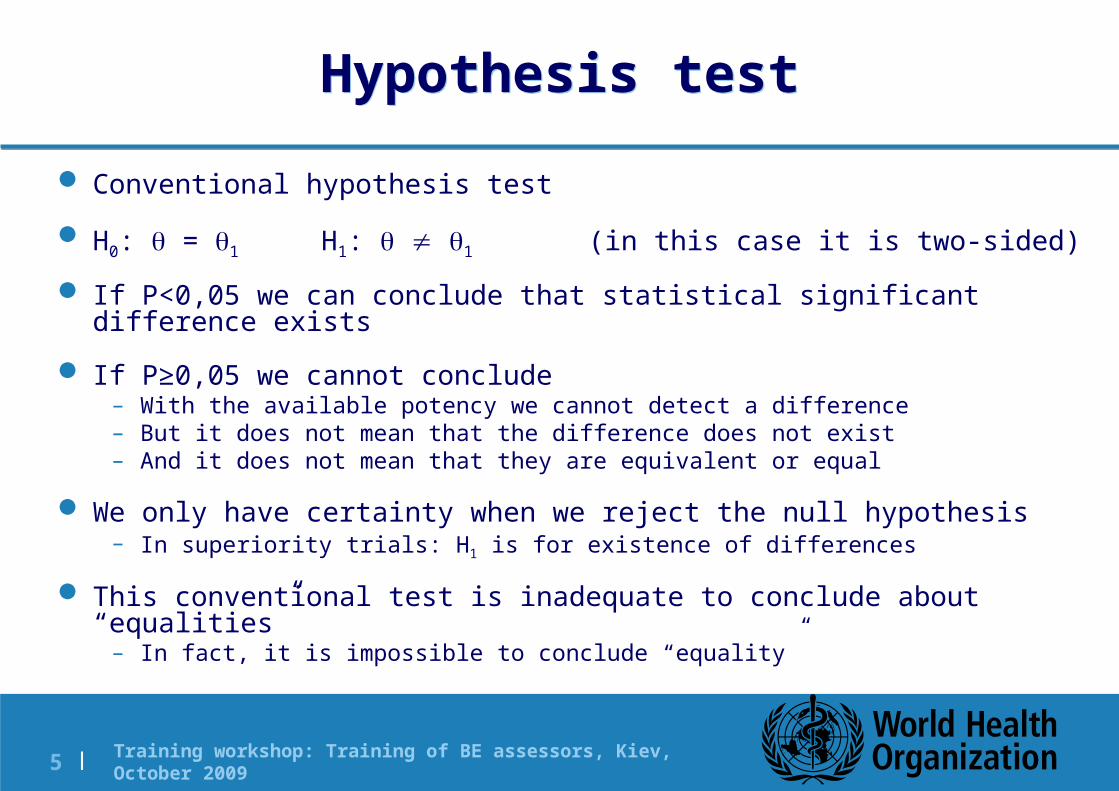
Hypothesis testHypothesis test
Conventional hypothesis test
H0: = 1 H1: 1 (in this case it is two-sided)
If P<0,05 we can conclude that statistical significant difference exists
If P≥0,05 we cannot conclude– With the available potency we cannot detect a difference– But it does not mean that the difference does not exist– And it does not mean that they are equivalent or equal
We only have certainty when we reject the null hypothesis– In superiority trials: H1 is for existence of differences
This conventional test is inadequate to conclude about “equalities”– In fact, it is impossible to conclude “equality”

Training workshop: Training of BE assessors, Kiev, October 20096 |
Null vs. Alternative hypothesisNull vs. Alternative hypothesis
Fisher, R.A. The Design of Experiments, Oliver and Boyd, London, 1935
“The null hypothesis is never proved or established, but is possibly disproved in the course of experimentation. Every experiment may be said to exist only in order to give the facts a chance of disproving the null hypothesis”
Frequent mistake: The absence of statistical significance has been interpreted incorrectly as absence of clinically relevant differences.

Training workshop: Training of BE assessors, Kiev, October 20097 |
EquivalenceEquivalence
We are interested in verifying (instead of rejecting) the null hypothesis of a conventional hypothesis test
We have to redefine the alternative hypothesis as a range of values with an equivalent effect
The differences within this range are considered clinically irrelevant
Problem: it is very difficult to define the maximum difference without clinical relevance for the Cmax and AUC of each drug
Solution: 20% based on a survey among physicians

Training workshop: Training of BE assessors, Kiev, October 20098 |
Interval hypothesis or two one-sided testsInterval hypothesis or two one-sided tests
Redefine the null hypothesis: How?
Solution: It is like changing the null to the alternative hypothesis and vice versa.
Alternative hypothesis test: Schuirmann, 1981– H01: 1 Ha1: 1<– H02: 2 Ha2: < 2.
This is equivalent to:– H0: 1 or 2 Ha: 1<<2
It is called as an interval hypothesis because the equivalence hypothesis is in the alternative hypothesis and it is expressed as an interval

Training workshop: Training of BE assessors, Kiev, October 20099 |
Interval hypothesis or two one-sided testsInterval hypothesis or two one-sided tests
The new alternative hypothesis is decided with a statistic that follows a distribution that can be approximated to a t-distribution
To conclude bioequivalence a P value <0.05 has to be obtained in both one-sided tests
The hypothesis tests do not give an idea of magnitude of equivalence (P<0001 vs. 90% CI: 0.95 – 1.05).
That is why confidence intervals are preferred

Training workshop: Training of BE assessors, Kiev, October 200910 |
Point estimate of the differencePoint estimate of the difference
If T=R, d=T-R=0
If T>R, d=T-R>0
If T<R, d=T-R<0
d < 0Negative effect
d = 0No difference
d > 0Positive effect

Training workshop: Training of BE assessors, Kiev, October 200911 |
Estimation with confidence intervals in a superiority trial
Estimation with confidence intervals in a superiority trial
d < 0Negative effect
d = 0No difference
d > 0Positive effect
Confidence interval 90% - 95%
It is not statistically significant!
Because the CI includes the d=0 value

Training workshop: Training of BE assessors, Kiev, October 200912 |
Estimation with confidence intervals in a superiority trial
Estimation with confidence intervals in a superiority trial
d < 0Negative effect
d = 0No difference
d > 0Positive effect
Confidence interval 90% - 95%
It is statistically significant!Because the CI does not includes the d=0 value
Training workshop: Training of BE assessors, Kiev, October 200913 |
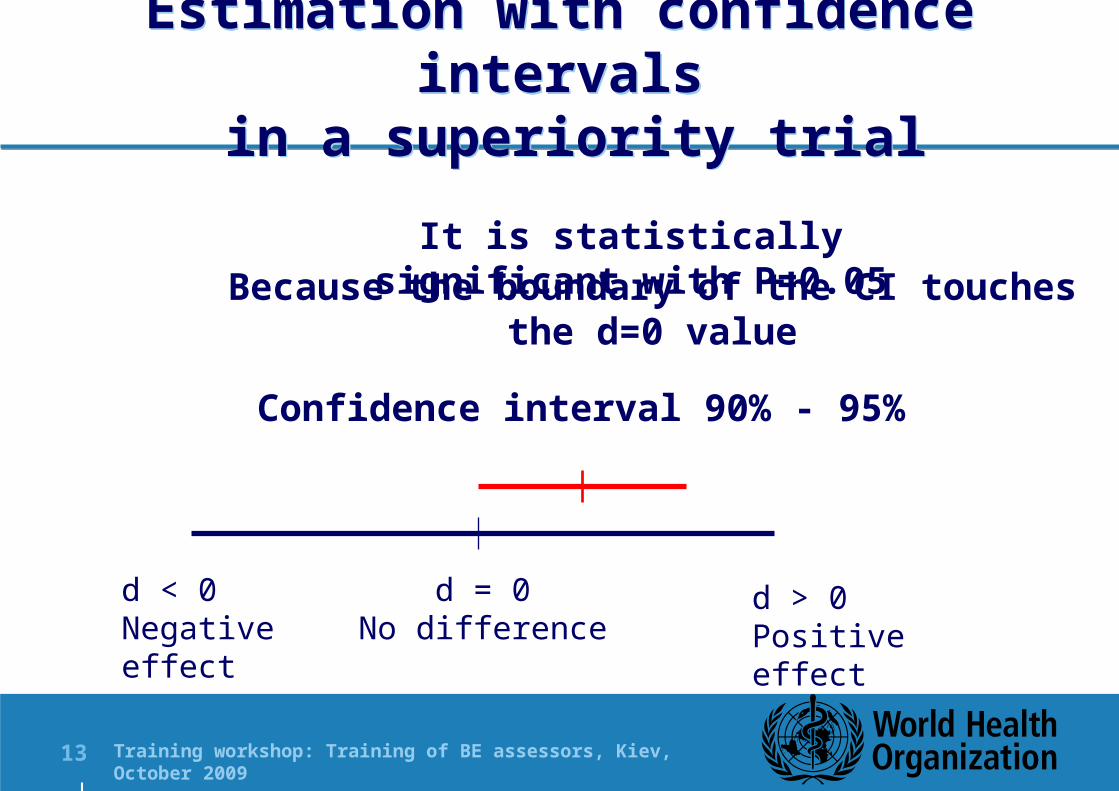
Estimation with confidence intervals in a superiority trial
Estimation with confidence intervals in a superiority trial
d < 0Negative effect
d = 0No difference
d > 0Positive effect
Confidence interval 90% - 95%
It is statistically significant with P=0.05Because the boundary of the CI touches the d=0 value

Training workshop: Training of BE assessors, Kiev, October 200914 |
Equivalence studyEquivalence study
d < 0Negative effect
d = 0No difference
d > 0Positive effect
- +
Region of clinical
equivalence

Training workshop: Training of BE assessors, Kiev, October 200915 |
Equivalence vs. differenceEquivalence vs. difference
d < 0Negative effect
d = 0No difference
d > 0Positive effect
- +
Region of clinical equivalenceEquivalent? Different?
No?
YesYes
Yes?
?
YesYes
Yes
YesYes
Yes?
?
No

Training workshop: Training of BE assessors, Kiev, October 200916 |
Non-inferiority studyNon-inferiority study
d < 0Negative effect
d = 0No difference
d > 0Positive effect
-
Inferiority limitInferior?
Yes?
NoNo
NoNo
?
No

Training workshop: Training of BE assessors, Kiev, October 200917 |
Superiority study (?)Superiority study (?)
d < 0Negative effect
d = 0No difference
d > 0Positive effect
+
Superiority limitSuperior?
No, not clinically, but yes statistically?, but yes statistically
Yes, statistical & clinically
NoNo
NoNo, not clinically and ? statistically
?
Yes, but only the point estimate

Training workshop: Training of BE assessors, Kiev, October 200918 |
How to perform the statistical analysis of a 2x2 cross-over bioequivalence study
How to perform the statistical analysis of a 2x2 cross-over bioequivalence study

Training workshop: Training of BE assessors, Kiev, October 200919 |
Statistical Analysis of BE studiesStatistical Analysis of BE studies
Sponsors have to use validated software– E.g. SAS, SPSS, Winnonlin, etc.
In the past, it was possible to find statistical analyses performed with incorrect software.– Calculations based on arithmetic means, instead of
Least Square Means, give biased results in unbalanced studies
• Unbalance: different number of subjects in each sequence– Calculations for replicate designs are more
complex and prone to mistakes

Training workshop: Training of BE assessors, Kiev, October 200920 |
The statistical analysis is not so complexThe statistical analysis is not so complex
2x2 BE trial
N=12
Period 1Period 2
Sequence 1 (BA)
BA is RT
Y11Y12
Sequence 2 (AB)
AB is TR
Y21Y22

Training workshop: Training of BE assessors, Kiev, October 200921 |
We don’t need to calculate an ANOVA table We don’t need to calculate an ANOVA table
Sources of variation d. f. SS MS F P Inter-subject 23 16487,49 716,85 4,286 Carry-over 1 276,00 276,00 0,375 0,5468 Residual / subjects 22 16211,49 736,89 4,406 0,0005
Intra-subject 3778,19 Formulation 1 62,79 62,79 0,375 0,5463 Period 1 35,97 35,97 0,215 0,6474 Residual 22 3679,43 167,25
Total 47 20265,68

Training workshop: Training of BE assessors, Kiev, October 200922 |
With complex formulaeWith complex formulae
22
1 1····
22
1
2
1 1·
22
1
2
1 1···
2
k
n
ikiBetween
k j
n
ikiijkWithin
k j
n
iijkTotal
k
k
k
YYSS
YYSS
YYSS

Training workshop: Training of BE assessors, Kiev, October 200923 |
More complex formulaeMore complex formulae
2
1
2··
2
1 1
2·
221·11·22·12·
21
21
int
22
2
k k
k
k
n
i
kiInter
Carry
erCarryBetween
n
YYSS
YYYYnn
nnSS
SSSSSS
k

Training workshop: Training of BE assessors, Kiev, October 200924 |
And really complex formulaeAnd really complex formulae
2
1
2
1 1
2
1 1
2
1
2
1
2··
2
1
2·
2·2
2
22·12·11·21·21
21
2
12·22·11·21·21
21
22
2
12
2
12
k j
n
i k
n
i k k k
k
j k
jkkiijkIntra
Period
Drug
IntraPeriodDrugWithin
k k
n
Y
n
YYYSS
YYYYnn
nnSS
YYYYnn
nnSS
SSSSSSSS

Training workshop: Training of BE assessors, Kiev, October 200925 |
Given the following data, it is simpleGiven the following data, it is simple
2x2 BE trial
N=12
Period 1Period 2
Sequence 1 (BA)Y11
75, 95, 90, 80, 70, 85
Y12
70, 90, 95, 70, 60, 70
Sequence 2 (AB)Y21
75, 85, 80, 90, 50, 65
Y22
40, 50, 70, 80, 70, 95
Training workshop: Training of BE assessors, Kiev, October 200926 |
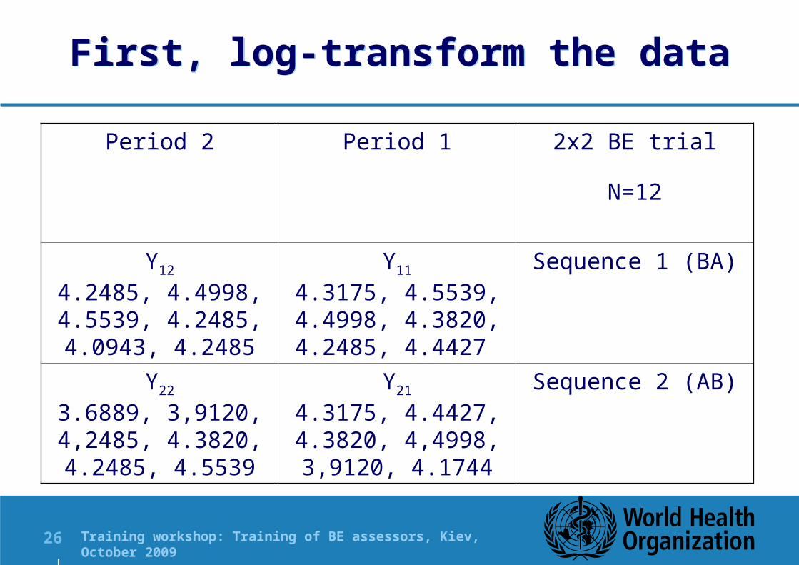
First, log-transform the dataFirst, log-transform the data
2x2 BE trial
N=12
Period 1Period 2
Sequence 1 (BA)Y11
4.3175, 4.5539, 4.4998, 4.3820, 4.2485, 4.4427
Y12
4.2485, 4.4998, 4.5539, 4.2485, 4.0943, 4.2485
Sequence 2 (AB)Y21
4.3175, 4.4427, 4.3820, 4,4998, 3,9120, 4.1744
Y22
3.6889, 3,9120, 4,2485, 4.3820, 4.2485, 4.5539

Training workshop: Training of BE assessors, Kiev, October 200927 |
Second, calculate the arithmetic mean of each period and sequence
Second, calculate the arithmetic mean of each period and sequence
2x2 BE trial
N=12
Period 1Period 2
Sequence 1 (BA)Y11 = 4.407Y12 = 4.316
Sequence 2 (AB)Y21 = 4.288Y22 = 4,172

Training workshop: Training of BE assessors, Kiev, October 200928 |
Note the difference between Arithmetic Mean and Least Square Mean
Note the difference between Arithmetic Mean and Least Square Mean
The arithmetic mean (AM) of T (or R) is the mean of all observations with T (or R) irrespective of its group or sequence
– All observations have the same weight
The LSM of T (or R) is the mean of the two sequence by period means
– In case of balanced studies AM = LSM – In case of unbalanced studies observations in sequences with
less subjects have more weight– In case of a large unbalance between sequences due to drop-
outs or withdrawals the bias of the AM is notable

Training workshop: Training of BE assessors, Kiev, October 200929 |
Third, calculate the LSM of T and RThird, calculate the LSM of T and R
2x2 BE trial
N=12
Period 1Period 2
Sequence 1 (BA)Y11 = 4.407Y12 = 4.316
Sequence 2 (AB)Y21 = 4.288Y22 = 4,172
B = 4.2898 A = 4.3018

Training workshop: Training of BE assessors, Kiev, October 200930 |
Fourth, calculate the point estimateFourth, calculate the point estimate
F = LSM Test (A) – LSM Reference (B)
F = 4.30183 – 4.28985 = 0.01198
Fifth step! Back-transform to the original scale
Point estimate = eF = e0.01198 = 1.01205
Five very simple steps to calculate the point estimate!!!

Training workshop: Training of BE assessors, Kiev, October 200931 |
Now we need to calculate the variability!Now we need to calculate the variability!
Step 1: Calculate the difference between periods for each subject and divide it by 2: (P2-P1)/2
Step 2: Calculate the mean of these differences within each sequence to obtain 2 means: d1 and d2
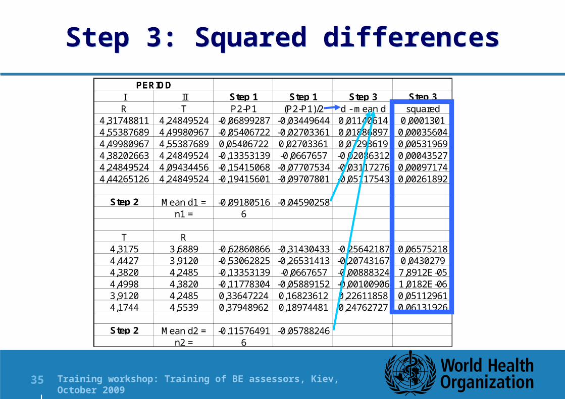
Step 3:Calculate the difference between “the difference in each subject” and “its corresponding sequence mean”. And square it.
Step 4: Sum these squared differences
Step 5: Divide it by (n1+n2-2), where n1 and n2 is the number of subjects in each sequence. In this example 6+6-2 = 10
– This value multiplied by 2 is the MSE– CV (%) = 100 x √eMSE-1

Training workshop: Training of BE assessors, Kiev, October 200932 |
This can be done easily in a spreadsheet!This can be done easily in a spreadsheet!
I II Step 1 Step 1 Step 3 Step 3 Step 4R T P2-P1 (P2-P1)/2 d - mean d squared Sum = 0,23114064
4,31748811 4,24849524 -0,06899287 -0,03449644 0,01140614 0,00013014,55387689 4,49980967 -0,05406722 -0,02703361 0,01886897 0,00035604 Step 54,49980967 4,55387689 0,05406722 0,02703361 0,07293619 0,00531969 Sigma2(d) = 0,023114064,38202663 4,24849524 -0,13353139 -0,0667657 -0,02086312 0,00043527 MSE= 0,046228134,24849524 4,09434456 -0,15415068 -0,07707534 -0,03117276 0,00097174 CV = 21,75162184,44265126 4,24849524 -0,19415601 -0,09707801 -0,05117543 0,00261892
Step 2 Mean d1 = -0,09180516 -0,04590258n1 = 6
T R4,3175 3,6889 -0,62860866 -0,31430433 -0,25642187 0,065752184,4427 3,9120 -0,53062825 -0,26531413 -0,20743167 0,04302794,3820 4,2485 -0,13353139 -0,0667657 -0,00888324 7,8912E-054,4998 4,3820 -0,11778304 -0,05889152 -0,00100906 1,0182E-063,9120 4,2485 0,33647224 0,16823612 0,22611858 0,051129614,1744 4,5539 0,37948962 0,18974481 0,24762727 0,06131926
Step 2 Mean d2 = -0,11576491 -0,05788246n2 = 6
PERIOD

Training workshop: Training of BE assessors, Kiev, October 200933 |
Step 1: Calculate the difference between periods for each subject and divide it by 2: (P2-P1)/2
Step 1: Calculate the difference between periods for each subject and divide it by 2: (P2-P1)/2
I II Step 1 Step 1R T P2-P1 (P2-P1)/2
4,31748811 4,24849524 -0,06899287 -0,034496444,55387689 4,49980967 -0,05406722 -0,027033614,49980967 4,55387689 0,05406722 0,027033614,38202663 4,24849524 -0,13353139 -0,06676574,24849524 4,09434456 -0,15415068 -0,077075344,44265126 4,24849524 -0,19415601 -0,09707801
Step 2 Mean d1 = -0,09180516 -0,04590258n1 = 6
T R4,3175 3,6889 -0,62860866 -0,314304334,4427 3,9120 -0,53062825 -0,265314134,3820 4,2485 -0,13353139 -0,06676574,4998 4,3820 -0,11778304 -0,058891523,9120 4,2485 0,33647224 0,168236124,1744 4,5539 0,37948962 0,18974481
Step 2 Mean d2 = -0,11576491 -0,05788246n2 = 6
PERIOD

Training workshop: Training of BE assessors, Kiev, October 200934 |
Step 2: Calculate the mean of these differences within each sequence to obtain 2 means: d1 & d2Step 2: Calculate the mean of these differences
within each sequence to obtain 2 means: d1 & d2
I II Step 1 Step 1R T P2-P1 (P2-P1)/2
4,31748811 4,24849524 -0,06899287 -0,034496444,55387689 4,49980967 -0,05406722 -0,027033614,49980967 4,55387689 0,05406722 0,027033614,38202663 4,24849524 -0,13353139 -0,06676574,24849524 4,09434456 -0,15415068 -0,077075344,44265126 4,24849524 -0,19415601 -0,09707801
Step 2 Mean d1 = -0,09180516 -0,04590258n1 = 6
T R4,3175 3,6889 -0,62860866 -0,314304334,4427 3,9120 -0,53062825 -0,265314134,3820 4,2485 -0,13353139 -0,06676574,4998 4,3820 -0,11778304 -0,058891523,9120 4,2485 0,33647224 0,168236124,1744 4,5539 0,37948962 0,18974481
Step 2 Mean d2 = -0,11576491 -0,05788246n2 = 6
PERIOD
Training workshop: Training of BE assessors, Kiev, October 200935 |
I II Step 1 Step 1 Step 3 Step 3R T P2-P1 (P2-P1)/2 d - mean d squared
4,31748811 4,24849524 -0,06899287 -0,03449644 0,01140614 0,00013014,55387689 4,49980967 -0,05406722 -0,02703361 0,01886897 0,000356044,49980967 4,55387689 0,05406722 0,02703361 0,07293619 0,005319694,38202663 4,24849524 -0,13353139 -0,0667657 -0,02086312 0,000435274,24849524 4,09434456 -0,15415068 -0,07707534 -0,03117276 0,000971744,44265126 4,24849524 -0,19415601 -0,09707801 -0,05117543 0,00261892
Step 2 Mean d1 = -0,09180516 -0,04590258n1 = 6
T R4,3175 3,6889 -0,62860866 -0,31430433 -0,25642187 0,065752184,4427 3,9120 -0,53062825 -0,26531413 -0,20743167 0,04302794,3820 4,2485 -0,13353139 -0,0667657 -0,00888324 7,8912E-054,4998 4,3820 -0,11778304 -0,05889152 -0,00100906 1,0182E-063,9120 4,2485 0,33647224 0,16823612 0,22611858 0,051129614,1744 4,5539 0,37948962 0,18974481 0,24762727 0,06131926
Step 2 Mean d2 = -0,11576491 -0,05788246n2 = 6
PERIOD
Step 3: Squared differencesStep 3: Squared differences

Training workshop: Training of BE assessors, Kiev, October 200936 |
Step 3 Step 4squared Sum = 0,23114064
0,00013010,00035604 Step 50,00531969 Sigma2(d) = 0,023114060,00043527 MSE= 0,046228130,00097174 CV = 21,75162180,00261892
0,065752180,04302797,8912E-051,0182E-060,051129610,06131926
Step 4: Sum these squared differencesStep 4: Sum these squared differences

Training workshop: Training of BE assessors, Kiev, October 200937 |
Step 3 Step 4squared Sum = 0,23114064
0,00013010,00035604 Step 50,00531969 Sigma2(d) = 0,023114060,00043527 MSE= 0,046228130,00097174 CV = 21,75162180,00261892
0,065752180,04302797,8912E-051,0182E-060,051129610,06131926
Step 5: Divide the sum by n1+n2-2Step 5: Divide the sum by n1+n2-2

Training workshop: Training of BE assessors, Kiev, October 200938 |
Calculate the confidence interval withpoint estimate and variability
Calculate the confidence interval withpoint estimate and variability
Step 11: In log-scale
90% CI: F ± t(0.1, n1+n2-2)-√((Sigma2(d) x (1/n1+1/n2))
F has been calculated before
The t value is obtained in t-Studient tables with 0,1 alpha and n1+n2-2 degrees of freedom
– Or in MS Excel with the formula =DISTR.T.INV(0.1; n1+n2-2)
Sigma2(d) has been calculated before.

Training workshop: Training of BE assessors, Kiev, October 200939 |
Final calculation: the 90% CIFinal calculation: the 90% CI
Log-scale 90% CI: F±t(0.1, n1+n2-2)-√((Sigma2(d)·(1/n1+1/n2))
F = 0.01198
t(0.1, n1+n2-2) = 1.8124611
Sigma2(d) = 0.02311406
90% CI: LL = -0.14711 to UL= 0,17107
Step 12: Back transform the limits with eLL and eUL
eLL = e-0.14711 = 0.8632 and eUL = e0.17107 = 1.1866

Training workshop: Training of BE assessors, Kiev, October 200940 |
How to calculate the sample size of a 2x2 cross-over bioequivalence study
How to calculate the sample size of a 2x2 cross-over bioequivalence study
Training workshop: Training of BE assessors, Kiev, October 200941 |
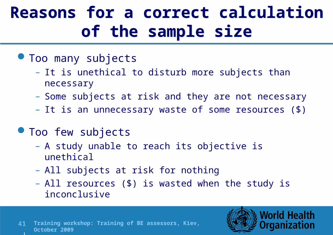
Reasons for a correct calculation of the sample size
Reasons for a correct calculation of the sample size
Too many subjects– It is unethical to disturb more subjects than necessary– Some subjects at risk and they are not necessary– It is an unnecessary waste of some resources ($)
Too few subjects– A study unable to reach its objective is unethical– All subjects at risk for nothing – All resources ($) is wasted when the study is inconclusive

Training workshop: Training of BE assessors, Kiev, October 200942 |
Frequent mistakesFrequent mistakes
To calculate the sample size required to detect a 20% difference assuming that treatments are e.g. equal
– Pocock, Clinical Trials, 1983
To use calculation based on data without log-transformation
– Design and Analysis of Bioavailability and Bioequivalence Studies, Chow & Liu, 1992 (1st edition) and 2000 (2nd edition)
Too many extra subjects. Usually no need of more than 10%. Depends on tolerability
– 10% proposed by Patterson et al, Eur J Clin Pharmacol 57: 663-670 (2001)

Training workshop: Training of BE assessors, Kiev, October 200943 |
Methods to calculate the sample sizeMethods to calculate the sample size
Exact value has to be obtained with power curves
Approximate values are obtained based on formulae– Best approximation: iterative process (t-test)– Acceptable approximation: based on Normal distribution
Calculations are different when we assume products are really equal and when we assume products are slightly different
Any minor deviation is masked by extra subjects to be included to compensate drop-outs and withdrawals (10%)

Training workshop: Training of BE assessors, Kiev, October 200944 |
Calculation assuming thattreatments are equal
Calculation assuming thattreatments are equal
Z(1-(/2)) = DISTR.NORM.ESTAND.INV(0.05) for 90% 1-
Z(1-(/2)) = DISTR.NORM.ESTAND.INV(0.1) for 80% 1-
Z(1-) = DISTR.NORM.ESTAND.INV(0.05) for 5%
2
2121
2
25.1
2
Ln
ZZsN w
22 1 CVLnsw CV expressed as 0.3 for 30%

Training workshop: Training of BE assessors, Kiev, October 200945 |
Example of calculation assuming thattreatments are equal
Example of calculation assuming thattreatments are equal
If we desire a 80% power, Z(1-(/2)) = -1.281551566
Consumer risk always 5%, Z(1-) = -1.644853627
The equation becomes: N = 343.977655 x S2
Given a CV of 30%, S2 = 0,086177696
Then N = 29,64
We have to round up to the next pair number: 30
Plus e.g. 4 extra subject in case of drop-outs
Training workshop: Training of BE assessors, Kiev, October 200946 |
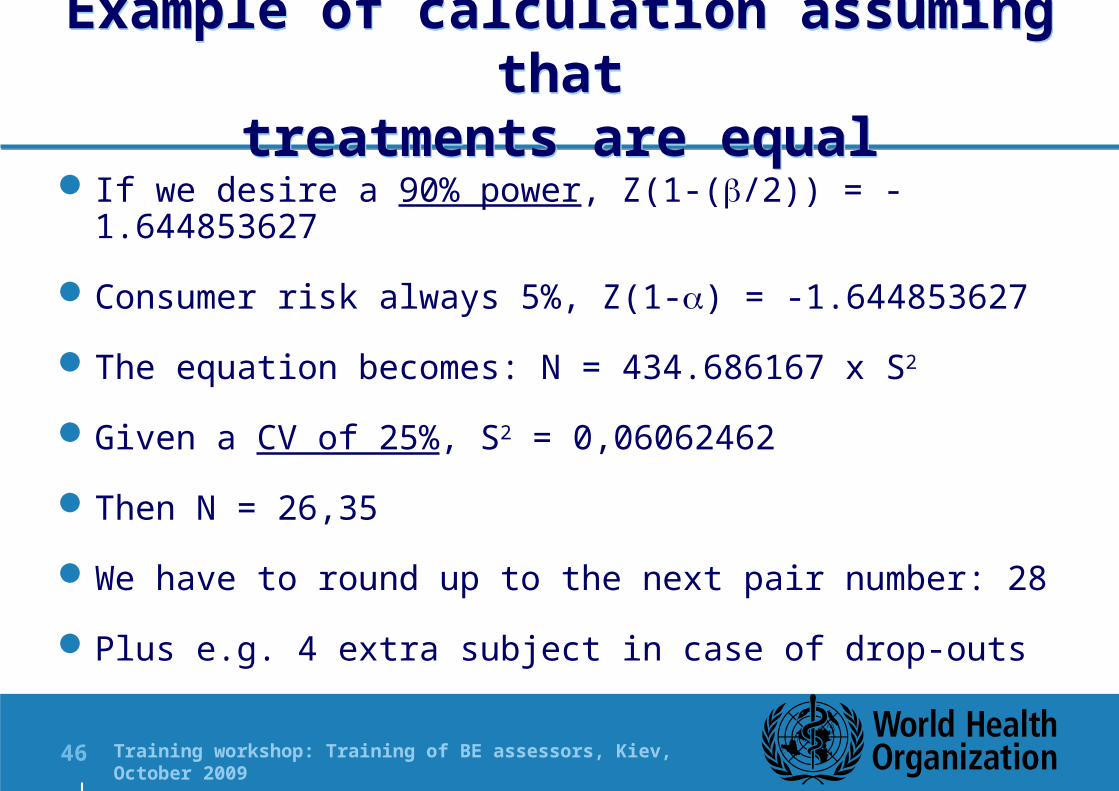
Example of calculation assuming thattreatments are equal
Example of calculation assuming thattreatments are equal
If we desire a 90% power, Z(1-(/2)) = -1.644853627
Consumer risk always 5%, Z(1-) = -1.644853627
The equation becomes: N = 434.686167 x S2
Given a CV of 25%, S2 = 0,06062462
Then N = 26,35
We have to round up to the next pair number: 28
Plus e.g. 4 extra subject in case of drop-outs

Training workshop: Training of BE assessors, Kiev, October 200947 |
Calculation assuming thattreatments are not equal
Calculation assuming thattreatments are not equal
2
211
2
25.1
2
LnLn
ZZsN
RT
w
1RT
Z(1-) = DISTR.NORM.ESTAND.INV(0.1) for 90% 1-b
Z(1-) = DISTR.NORM.ESTAND.INV(0.2) for 80% 1-b
Z(1-) = DISTR.NORM.ESTAND.INV(0.05) for 5% a

Training workshop: Training of BE assessors, Kiev, October 200948 |
Example of calculation assuming thattreatments are 5% different
Example of calculation assuming thattreatments are 5% different
If we desire a 90% power, Z(1-) = -1.28155157
Consumer risk always 5%, Z(1-) = -1.644853627
If we assume thatT/R=1.05
The equation becomes: N = 563.427623 x S2
Given a CV of 40 %, S2 = 0,14842001
Then N = 83.62
We have to round up to the next pair number: 84
Plus e.g. 8 extra subject in case of drop-outs

Training workshop: Training of BE assessors, Kiev, October 200949 |
Example of calculation assuming thattreatments are 5% different
Example of calculation assuming thattreatments are 5% different
If we desire a 80% power, Z(1-) = -0.84162123
Consumer risk always 5%, Z(1-) = -1.644853627
If we assume thatT/R=1.05
The equation becomes: N = 406.75918 x S2
Given a CV of 20 %, S2 = 0,03922071
Then N = 15.95
We have to round up to the next pair number: 16
Plus e.g. 2 extra subject in case of drop-outs

Training workshop: Training of BE assessors, Kiev, October 200950 |
Example of calculation assuming thattreatments are 10% different
Example of calculation assuming thattreatments are 10% different
If we desire a 80% power, Z(1-) = -0.84162123
Consumer risk always 5%, Z(1-) = -1.644853627
If we assume thatT/R=1.11
The equation becomes: N = 876.366247 x S2
Given a CV of 20 %, S2 = 0,03922071
Then N = 34.37
We have to round up to the next pair number: 36
Plus e.g. 4 extra subject in case of drop-outs

Training workshop: Training of BE assessors, Kiev, October 200951 |
How to calculate the CVbased on the 90% CI of a BE study
How to calculate the CVbased on the 90% CI of a BE study

Training workshop: Training of BE assessors, Kiev, October 200952 |
Example of calculation of the CV based on the 90% CIExample of calculation of
the CV based on the 90% CI
Given a 90% CI: 82.46 to 111.99 in BE study with N=24
Log-transform the 90% CI: 4.4123 to 4.7184
The mean of these extremes is the point estimate: 4.5654
Back-transform to the original scale e4.5654 = 96.08
The width in log-scale is 4.7184 – 4.5654 = 0,1530
With the sample size calculate the t-value. How?– Based on the Student-t test tables or a computer (MS Excel)

Training workshop: Training of BE assessors, Kiev, October 200953 |
Example of calculation of the CV based on the 90% CIExample of calculation of
the CV based on the 90% CI
Given a N = 24, the degrees of freedom are 22
t = DISTR.T.INV(0.1;n-2) = 1.7171
Standard error of the difference (SE(d)) = Width / t-value = 0.1530 / 1.7171 = 0,0891
Square it: 0.08912 = 0,0079 and divide it by 2 = 0,0040
Multiply it by the sample size: 0.0040x24 = 0,0953 = MSE
CV (%) = 100 x √(eMSE-1) = 100 x √(e0.0953-1) = 31,63 %