
STATISTICAL CONCEPTS OF LQAS - danstan.com · STATISTICAL CONCEPTS OF LQAS Danstan Bagenda PhD...
109
STATISTICAL CONCEPTS OF LQAS Danstan Bagenda PhD Makerere University - School of Public Health May 12 2010 1
-
Upload
phunghuong -
Category
Documents
-
view
245 -
download
0
Transcript of STATISTICAL CONCEPTS OF LQAS - danstan.com · STATISTICAL CONCEPTS OF LQAS Danstan Bagenda PhD...

STATISTICAL CONCEPTS OF LQAS
Danstan Bagenda PhD
Makerere University - School of Public Health
May 12 2010
1

_____________________________Danstan Bagenda PhD May 2010 MUSPH
Some Background Concepts
• Back to Basics.......
2

_____________________________Danstan Bagenda PhD May 2010 MUSPH
Outline• Sampling
• Probability
• Probability distributions
• Binomial Distribution
• Hypothesis Testing (Estimation)
• Sample size
• How does LQAS fit in under these?
3

_____________________________Danstan Bagenda PhD May 2010 MUSPH
Sampling.....
4

_____________________________Danstan Bagenda PhD May 2010 MUSPH
Collections of ‘items’ is so LARGE!!
So Hard to get info!
• Voting populations - what % favors DP, FDC, NRM, UPC etc
• Manufactured goods - What % will be defective
• Uganda popn - what % HIV infected
5
_____________________________Danstan Bagenda PhD May 2010 MUSPH
Solution: Take a SAMPLE
• A relatively small subset of the total population
6
_____________________________Danstan Bagenda PhD May 2010 MUSPH
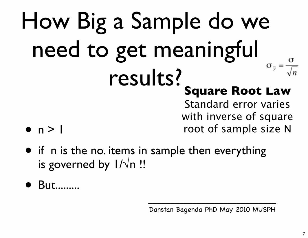
How Big a Sample do we need to get meaningful
results?
• n > 1
• if n is the no. items in sample then everything is governed by 1/√n !!
• But.........
Square Root Law Standard error varies with inverse of square root of sample size N
7

_____________________________Danstan Bagenda PhD May 2010 MUSPH
Sampling Design
• But QUALITY of sample as important its SIZE
• How do we assure ourselves that we are choosing a REPRESENTATIVE SAMPLE?
• The SELECTION PROCESS itself is critical
8

_____________________________Danstan Bagenda PhD May 2010 MUSPH
Sampling Design
• There are numerous ways to ruin & bias a sample
• Eg: selection of sample for HIV prevalence
9

_____________________________Danstan Bagenda PhD May 2010 MUSPH
Sampling Design
• The way to get statistically dependable results is to choose the sample at RANDOM
10

_____________________________Danstan Bagenda PhD May 2010 MUSPH
The Simple Random Sample (SRS)
• Suppose we have a large population of n people & a procedure of selecting n of them
• If procedure ensures that ALL POSSIBLE SAMPLES ARE EQUALLY LIKELY, then procedure is a SRS
11

_____________________________Danstan Bagenda PhD May 2010 MUSPH
The Simple Random Sample (SRS)
• A SRS has 2 properties:
• 1) UNBIASED: Each unit has the SAME chance of being chosen
• 2) INDEPENDENCE: Selection of one unit has NO INFLUENCE on the selection of other units
12
_____________________________Danstan Bagenda PhD May 2010 MUSPH
The Simple Random Sample (SRS)
• In Real World:
• Completely UNBIASED, INDEPENDENT samples hard to find
• Eg: How about if I randomly dial MTN, UTL, CELTEL, WARID, ORANGE numbers?
13
_____________________________Danstan Bagenda PhD May 2010 MUSPH
The Simple Random Sample (SRS)
• Eg: How about if I randomly dial MTN, UTL, CELTEL, WARID, ORANGE numbers?
• Ignores people without a telephone
• oversamples those with more than 1 telephone number
14
_____________________________Danstan Bagenda PhD May 2010 MUSPH
Sampling Frame
• Its theoretically possible to get a RANDOM SAMPLE by building a SAMPLING FRAME:
• List of every one (unit) in the population
• Use a RANDOM NUMBER GENERATOR (RNG) - we can pick n objects at random
• Stata: (Eg: “Pseudo”RNG )
15

_____________________________Danstan Bagenda PhD May 2010 MUSPH
Sampling Frame - (SRS)
• Equivalently,
• Put all names (numbers) on cards/papers
• Put all 11,919 papers in a drum/box
• Shake
• Close eyes & pick 500 of the cards/papers
16

_____________________________Danstan Bagenda PhD May 2010 MUSPH
Sampling Frame - (SRS)
• Not always easy/possible - Frame:
• may be prohibitively costly
• controversial (Kat chewers in Arua/other eg’s... PLSE?..)
• impossible - (eg: UW&SC = quality of water of UG lakes - What comprises a Lake?!! )
17
_____________________________Danstan Bagenda PhD May 2010 MUSPH
Sampling - other alternatives?
• More EFFICIENT & COST-EFFECTIVE alternatives to SRS?
• Yes
• If you already know something about population of interest
18

_____________________________Danstan Bagenda PhD May 2010 MUSPH
Stratified Sampling
• Divide the population units into HOMOGENOUS groups - (STRATA)
• Eg: Urban & Rural
• Men & Women
• Different Regions/Districts (West, Central, North & South)
• Draw a SRS from EACH group
19

_____________________________Danstan Bagenda PhD May 2010 MUSPH
Cluster Sampling
• Group the population into small CLUSTERS (eg, villages or parishes or counties)
• Draw a SRS of CLUSTERS
• Observe Everything in Sampled Clusters
• or MULTISTAGE (2-STAGE) - Take ANOTHER SRS from SAMPLED CLUSTERs
20

_____________________________Danstan Bagenda PhD May 2010 MUSPH
Cluster Sampling• Advantage:
• Reduces Travel costs
• Disadvantage:
• Less precise estimates likely
• people/units in same cluster likely similar to each other (non-independence!! - DESIGN EFFECT - (later)
21

_____________________________Danstan Bagenda PhD May 2010 MUSPH
Warning #1
• MOST Statistical Methods depend on:
• Independence
• Lack of bias
• on basis of Simple Random Sample (SRS) & apply ONLY to a SRS!!
• Other Sampling methods:
• Need RESULTS to be MODIFIED
22
_____________________________Danstan Bagenda PhD May 2010 MUSPH
Warning #2
• WITHOUT RANDOMIZED Design
• No dependable statistical analysis!
• NO MATTER HOW IT IS MODIFIED!
• RANDOM SAMPLING “STATISTICALLY GUARANTEES” accuracy of a survey
23

_____________________________Danstan Bagenda PhD May 2010 MUSPH
Probability....
24

_____________________________Danstan Bagenda PhD May 2010 MUSPH
Basic Definitions• RANDOM EXPERIMENT
• is the PROCESS of observing the OUTCOME of a CHANCE event. Egs Plse?
• ELEMENTARY OUTCOMES
• ALL POSSIBLE results of the random expt
• SAMPLE SPACE:
• SET or COLLECTION of ALL the ELEMENTARY outcomes
• EVENT - either a SINGLE OUTCOME or SET of OUTCOMES
25
_____________________________Danstan Bagenda PhD Nov 2009 MUSPH
Basic Definitions• Eg:
• If EVENT was “COIN TOSS”
• RANDOM EXPT consists of:
• RECORDING its OUTCOME
• The ELEMENTARY OUTCOMES are:
• HEADS (H) & TAILS (T)
• & SAMPLE SPACE is the set:
• {H,T}26
_____________________________Danstan Bagenda PhD Nov 2009 MUSPH
Basic Definitions• Eg:
• If EVENT was “THROW SINGLE DIE”
• & SAMPLE SPACE is the set:
• {1,2,3,4,5,6}
27

_____________________________Danstan Bagenda PhD Nov 2009 MUSPH
Basic Definitions• Eg:
• If EVENT was “THROW A PAIR OF DICE”
• & SAMPLE SPACE has 36 (6 x6) ELEMENTARY OUTCOMES:
28

_____________________________Danstan Bagenda PhD Nov 2009 MUSPH
Basic Definitions
29

_____________________________Danstan Bagenda PhD Nov 2009 MUSPH
Basic Definitions• Imagine: Random Expt with “n”
ELEMENTARY OUTCOMES:
• We want to assign a NUMERICAL WEIGHT or PROBABILITY to EACH OUTCOME
• -> measures the LIKELIHOOD of its occurring ie,
• We write:
• The PROBABILITY of as
O1, O2, . . . , On
Oi P (Oi)
30

_____________________________Danstan Bagenda PhD Nov 2009 MUSPH
Basic Definitions
• EG:
• In a FAIR COIN TOSS,
• HEADS & TAILS are EQUALLY likely & we assign them BOTH the probability 0.5:
• P(H) = P(T) = 0.5
• ie, each outcome comes up 1/2 the time
31
_____________________________Danstan Bagenda PhD Nov 2009 MUSPH
Approaches to Probability
• RELATIVE FREQUENCY:
• When an experiment CAN be REPEATED,
• then an EVENT’s PROBABILITY is:
• the PROPORTION OF TIMES THE EVENT occurs IN THE LONG RUN
• (BTW: EACH repetition in such an expt. is called a TRIAL)
32
_____________________________Danstan Bagenda PhD Nov 2009 MUSPH
Properties of Probability
• Probabilities are NEVER NEGATIVE
• A probability of ZERO means an event CANNOT HAPPEN
• A probability <0 is MEANINGLESS!!!!!!
P (Oi) ≥ 0
33

_____________________________Danstan Bagenda PhD Nov 2009 MUSPH
Properties of Probability
• If an event is CERTAIN to happen, we assign it a PROBABILITY 1 (In the long run, that’s the proportion of times it will occur!)
• In particular, the TOTAL PROBABILITY OF THE SAMPLE SPACE must BE 1
• ie, If we do the experiment, SOMETHING is bound to HAPPEN!!
•TOTAL PROBABILITY of ALL ELEMENTARY OUTCOMES IS ONE
P (Oi) + P (O2) + · · · + P (On) = 1
34
_____________________________Danstan Bagenda PhD May 2010 MUSPH
Probability Distributions....
35

_____________________________Danstan Bagenda PhD May 2010 MUSPH
Variable• The characteristic of interest in a study if
called a VARIABLE eg; weight of students in class
• Term VARIABLE makes sense because:
• value varies from subject to subject
• variation results from inherent biological variation among individuals
• errors made in measuring & recording subjects value on a characteristic
36
_____________________________Danstan Bagenda PhD May 2010 MUSPH
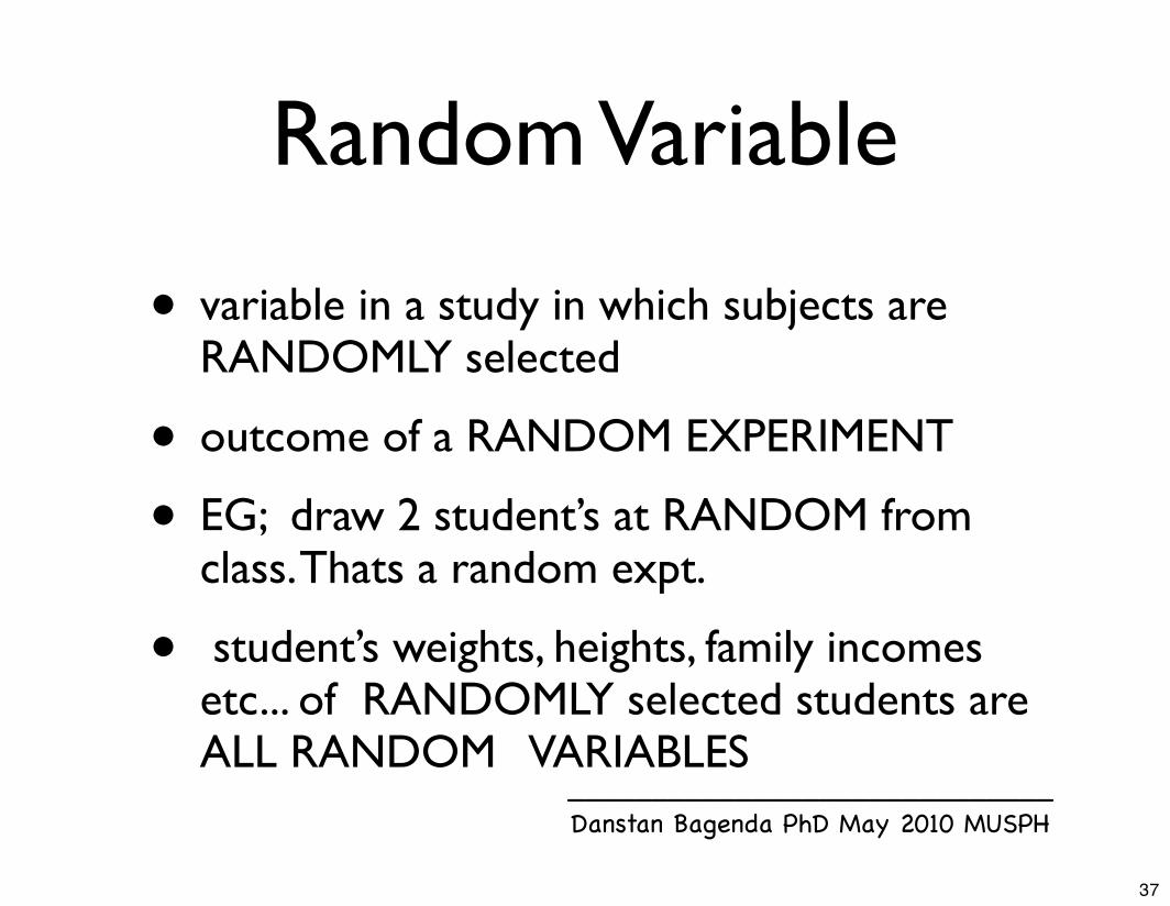
Random Variable
• variable in a study in which subjects are RANDOMLY selected
• outcome of a RANDOM EXPERIMENT
• EG; draw 2 student’s at RANDOM from class. Thats a random expt.
• student’s weights, heights, family incomes etc... of RANDOMLY selected students are ALL RANDOM VARIABLES
37

_____________________________Danstan Bagenda PhD May 2010 MUSPH
Random Variable• TOSS TWO COINS: (The Random Expt)
• Record the NO. OF HEADS (x) : 0, 1, or 2 (Random Variable)
Outcome TT HT or TH HH
x 0 1 2
38
_____________________________Danstan Bagenda PhD May 2010 MUSPH
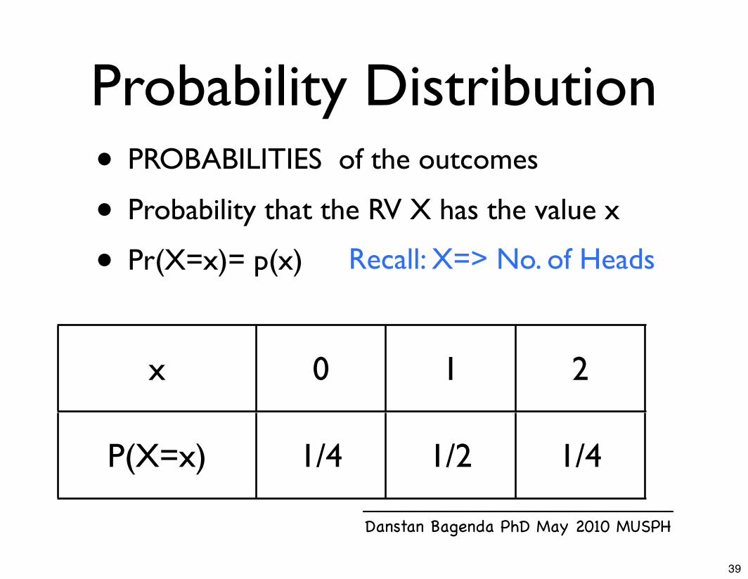
Probability Distribution• PROBABILITIES of the outcomes
• Probability that the RV X has the value x
• Pr(X=x)= p(x)
x 0 1 2
P(X=x) 1/4 1/2 1/4
Recall: X=> No. of Heads
39
_____________________________Danstan Bagenda PhD May 2010 MUSPH
Probability Distributions
• In some applications, a formula or rule will adequately describe the distribution
• In other situations, a theoretical distribution provides a good fit to the variable of interest
40
_____________________________Danstan Bagenda PhD May 2010 MUSPH
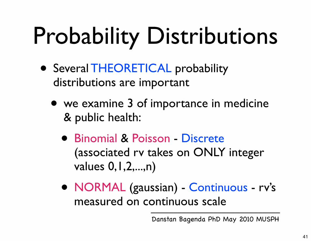
Probability Distributions• Several THEORETICAL probability
distributions are important
• we examine 3 of importance in medicine & public health:
• Binomial & Poisson - Discrete (associated rv takes on ONLY integer values 0,1,2,...,n)
• NORMAL (gaussian) - Continuous - rv’s measured on continuous scale
41

_____________________________Danstan Bagenda PhD May 2010 MUSPH
Binomial Distribution
• Event has only TWO possible OUTCOMEs
• eg: Head or Tails
• Success or Failure
• Characterized by 2 parameters:
• n = no. of independent trials
• p= probability of success of each trial
42

_____________________________Danstan Bagenda PhD May 2010 MUSPH
Binomial Distribution• Basic principles developed by Swiss
mathematician Jacob Bernoulli (1713)
• A repeatable Expt called a BERNOULLI TRIAL provided:
• 1) the result of each trial may either be a success or a failure
• 2) the probability p of success is the SAME in EVERY TRIAL
• 3) The trials are INDEPENDENT: the outcome of 1 trial has no influence on later outcomes
43
_____________________________Danstan Bagenda PhD May 2010 MUSPH
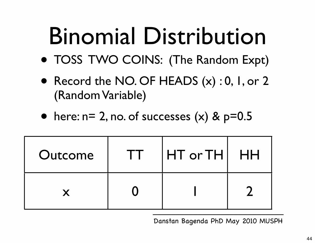
Binomial Distribution• TOSS TWO COINS: (The Random Expt)
• Record the NO. OF HEADS (x) : 0, 1, or 2 (Random Variable)
• here: n= 2, no. of successes (x) & p=0.5
Outcome TT HT or TH HH
x 0 1 2
44

_____________________________Danstan Bagenda PhD May 2010 MUSPH
Binomial Distribution
x 0 1 2
P(X=x) 1/4 1/2 1/4
45

_____________________________Danstan Bagenda PhD May 2010 MUSPH
Binomial Distribution
46

_____________________________Danstan Bagenda PhD May 2010 MUSPH
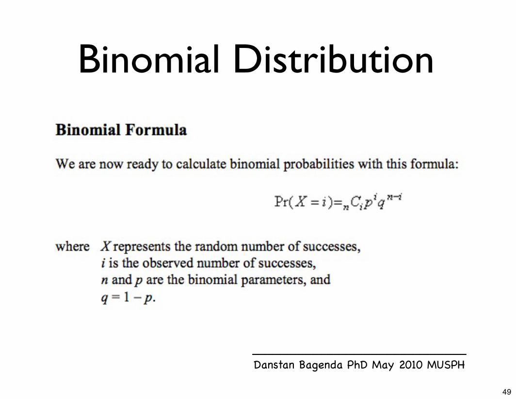
Binomial Distribution
nCi = n!i!(n−i)!
47

_____________________________Danstan Bagenda PhD May 2010 MUSPH
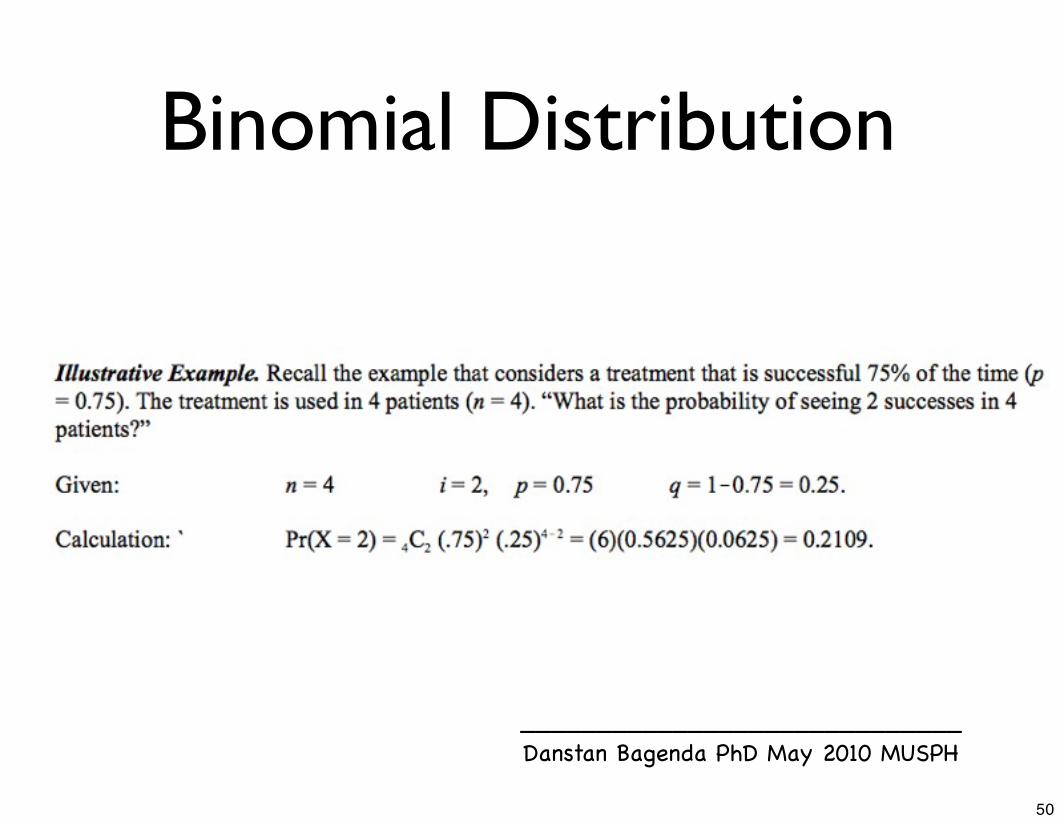
Binomial Distribution
48
_____________________________Danstan Bagenda PhD May 2010 MUSPH
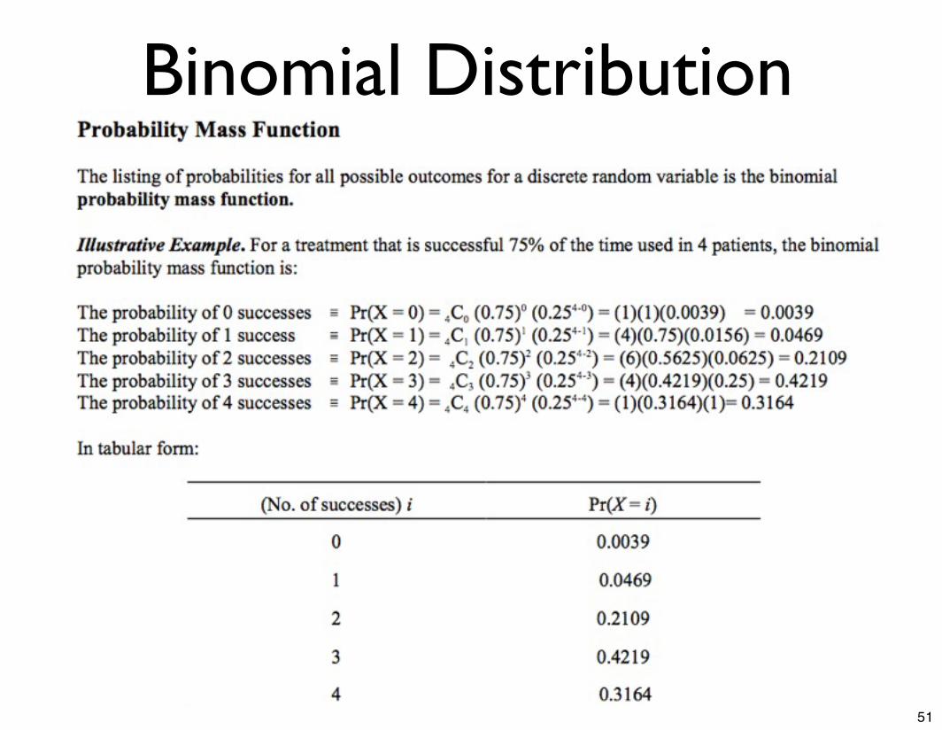
Binomial Distribution
49
_____________________________Danstan Bagenda PhD May 2010 MUSPH
Binomial Distribution
50
_____________________________Danstan Bagenda PhD May 2010 MUSPH
Binomial Distribution
51
_____________________________Danstan Bagenda PhD May 2010 MUSPH
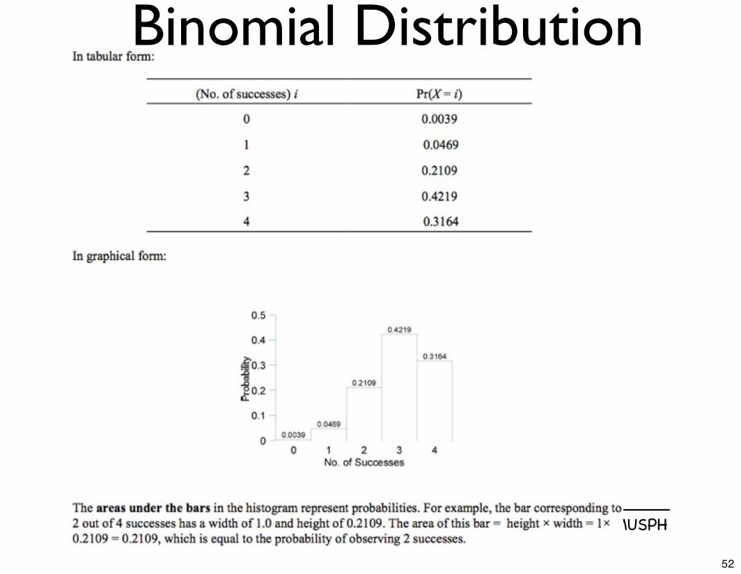
Binomial Distribution
52
_____________________________Danstan Bagenda PhD May 2010 MUSPH
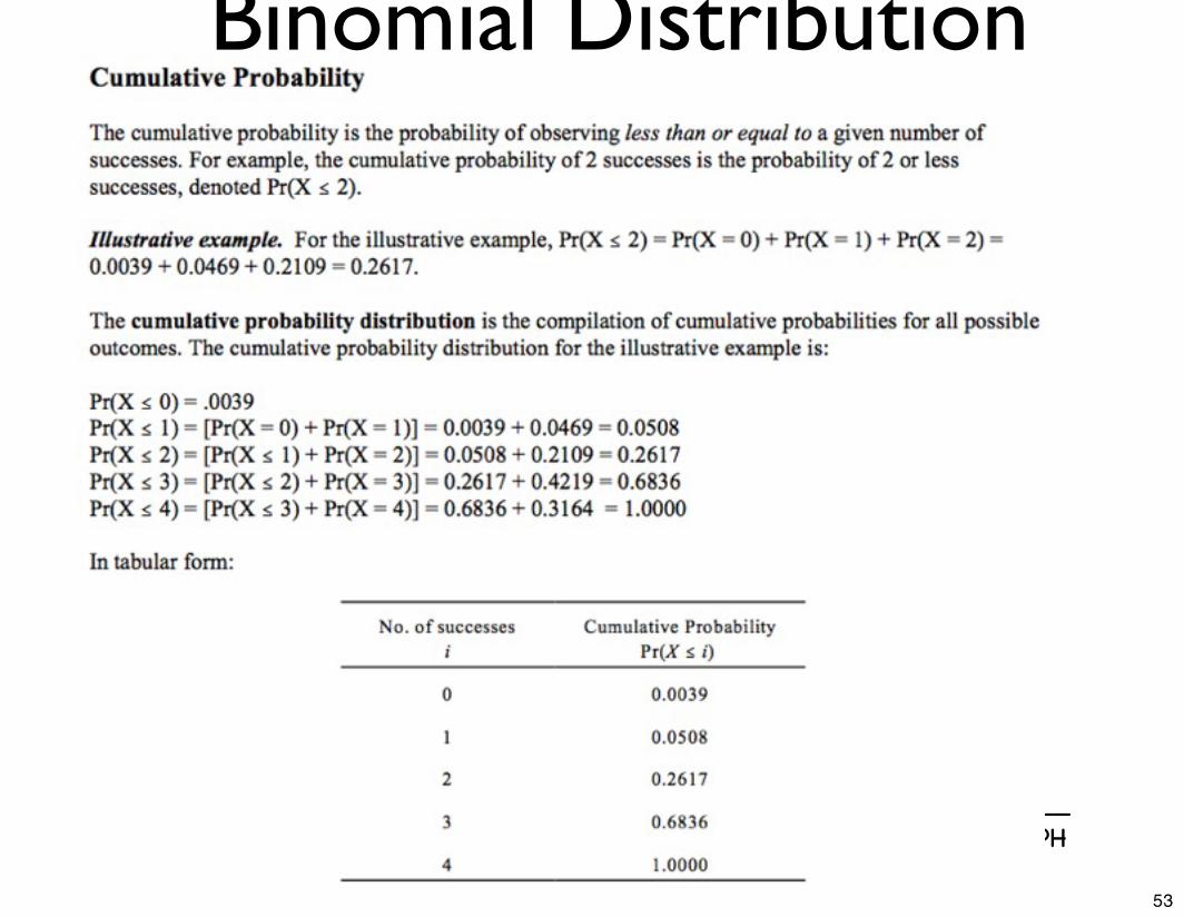
Binomial Distribution
53
_____________________________Danstan Bagenda PhD May 2010 MUSPH
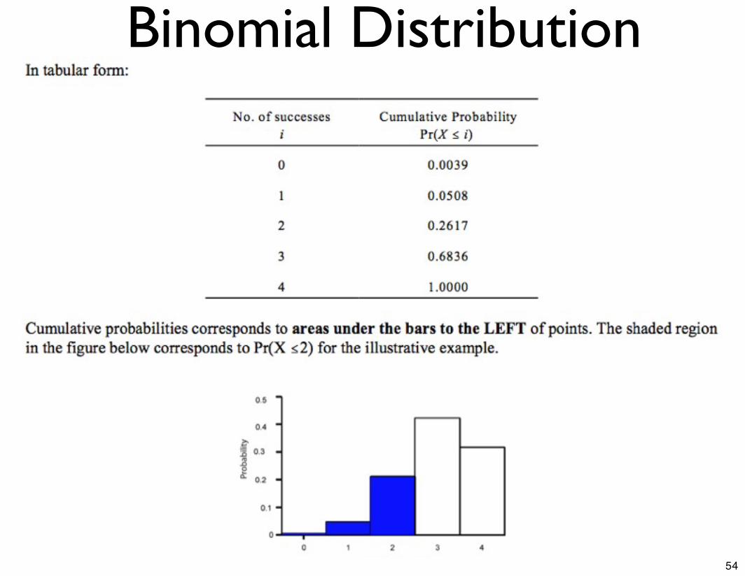
Binomial Distribution
54

_____________________________Danstan Bagenda PhD May 2010 MUSPH
Poisson Distribution
• Named after French mathematician who derived it Simeon D. Poisson
• Like Binomial, it is DISCRETE
• Used to determine probability of RARE events
• Similar to Binomial except that n (no of trials is very large) & p (probability of success is very small)
• No. of cases of Ebola in a given popn
55

_____________________________Danstan Bagenda PhD May 2010 MUSPH
Poisson Distribution• RV - no. of times an event occurs in a given
time or space interval
• Probability of exactly x occurrences is given by:
• λ is value of BOTH the mean & variance of the Poisson distribution, &
• e is the base if the natural log (=2.718)
• NOTE: while binomial distribtn has 2 parameters “n” & “p”, poisson ONLY needs 1 “λ”.
P (X) = λxe−λ
X!
56
_____________________________Danstan Bagenda PhD May 2010 MUSPH
Statistical Inference
• Hypothesis testing.....
57
_____________________________Danstan Bagenda PhD May 2010 MUSPH
Statistical Inference• STATISTICAL INFERENCE is:
• the act of GENERALIZING from a SAMPLE to a POPULATION with a calculated degree of certainty
• 2 Primary forms of Statistical Inference
• Estimation
• Hypothesis Testing
58
_____________________________Danstan Bagenda PhD May 2010 MUSPH
Statistical Inference
• ESTIMATION:
• provides the most likely LOCATION of a population parameter, often with a built-in “MARGIN OF ERROR”
• HYPOTHESIS TESTING:
• provides a way to judge the NON-CHANCE occurrence of a finding
59
_____________________________Danstan Bagenda PhD May 2010 MUSPH
Statistical Inference (Eg)
• Suppose, Want to learn about prevalence of smoking in POPULATION based on prevalence of smoking in SAMPLE.
60
_____________________________Danstan Bagenda PhD May 2010 MUSPH
Statistical Inference (Eg)• IN a given study, final inference may be:
• “25% of the adult popn. smokes” (POINT ESTIMATION)
• “BETWEEN 20% & 30% of the popn. smokes” (INTERVAL ESTIMATION)
• We want to TEST whether the prevalence of smoking “HAS CHANGED over time” (HYPOTHESIS TESTING)
61

_____________________________Danstan Bagenda PhD May 2010 MUSPH
• The situation in a statistical problem is that there is a population of interest, and a quantity or aspect of that population that is of interest. This quantity is called a parameter. The value of this parameter is unknown.
• To learn about this parameter we take a sample from the population and compute an estimate of the parameter called a statistic.
62

_____________________________Danstan Bagenda PhD May 2010 MUSPH
Parameters & Estimates• A PARAMETER is the numeric characteristic
of the POPULATION you want to learn about Eg:
• population mean age at 1st sex or
• proportion (%) of population that is HIV+
• An ESTIMATE is a numerical characteristic of the SAMPLE that you have
• SAMPLE mean age at 1st sex
• proportion (%) of SAMPLE that is HIV+
63

_____________________________Danstan Bagenda PhD May 2010 MUSPH
Parameters & Estimates
• ALTHO’ the 2 are RELATED, they are NOT INTERCHANGABLE
• Eg: A POPULATION Mean is a PARAMETER & you can use the SAMPLE mean as an ESTIMATE of this PARAMETER
64
_____________________________Danstan Bagenda PhD May 2010 MUSPH
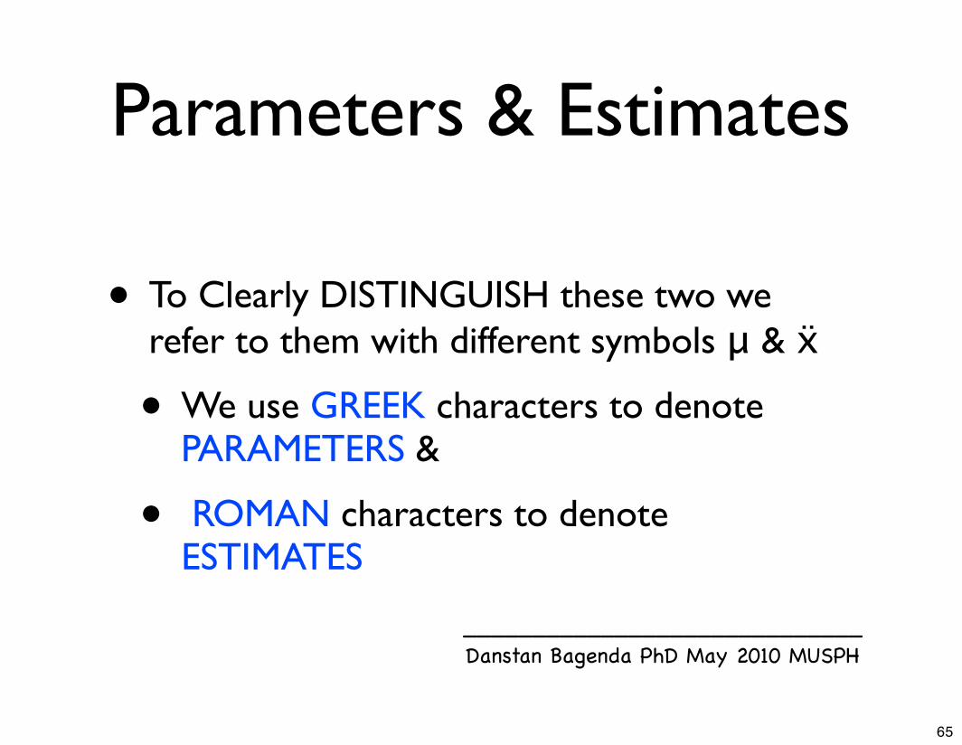
Parameters & Estimates
• To Clearly DISTINGUISH these two we refer to them with different symbols μ & ẍ
• We use GREEK characters to denote PARAMETERS &
• ROMAN characters to denote ESTIMATES
65

_____________________________Danstan Bagenda PhD May 2010 MUSPH
• A statistic is a number computed from a sample.
66

_____________________________Danstan Bagenda PhD May 2010 MUSPH
• A statistic is a number computed from a sample.
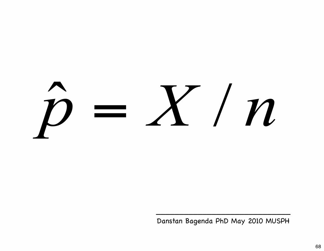
• The situation is that we are interested in the proportion of the population that has a certain characteristic.
• This proportion is the population parameter of interest, denoted by symbol p.
• We estimate this parameter with the statistic p-hat – the number in the sample with the characteristic divided by the sample size n.
67
_____________________________Danstan Bagenda PhD May 2010 MUSPH
68

_____________________________Danstan Bagenda PhD May 2010 MUSPH
Sampling Distribution of the Sample Proportion
Behavior of a simple sample statistic
69
_____________________________Danstan Bagenda PhD May 2010 MUSPH
Sampling Distribution of Proportions
• IMAGINE (PLEASE TRY!!!)
• Taking ALL POSSIBLE SAMPLES of SIZE n from a GIVEN POPULATION
• Then Take the proportion of each of these many samples.
• Then arrange these proportions to form a distribution
• THIS is what is meant by a SAMPLING DISTRIBUTION
70
_____________________________Danstan Bagenda PhD May 2010 MUSPH
• How does p-hat behave? To study the behavior, imagine taking many random samples of size n, and computing a p-hat for each of the samples.
• Then we plot this set of p-hats with a histogram.
71

_____________________________Danstan Bagenda PhD May 2010 MUSPH
72

_____________________________Danstan Bagenda PhD May 2010 MUSPH
• When sample sizes are fairly large, the shape of the p-hat distribution will be normal.
• The mean of the distribution is the value of the population parameter p.
• The standard deviation of this distribution is the square root of p(1-p)/n.
73

_____________________________Danstan Bagenda PhD May 2010 MUSPH
How does LQAS fit in?
74
_____________________________Danstan Bagenda PhD May 2010 MUSPH
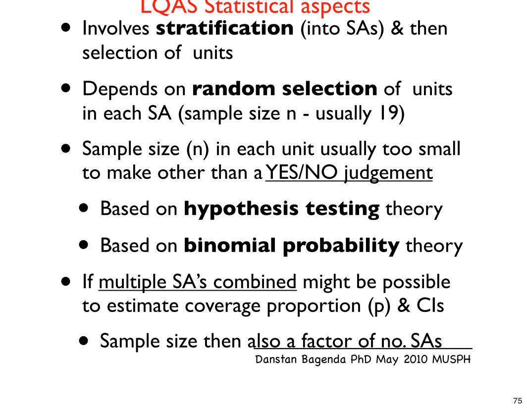
LQAS Statistical aspects• Involves stratification (into SAs) & then
selection of units
• Depends on random selection of units in each SA (sample size n - usually 19)
• Sample size (n) in each unit usually too small to make other than a YES/NO judgement
• Based on hypothesis testing theory
• Based on binomial probability theory
• If multiple SA’s combined might be possible to estimate coverage proportion (p) & CIs
• Sample size then also a factor of no. SAs
75
_____________________________Danstan Bagenda PhD May 2010 MUSPH
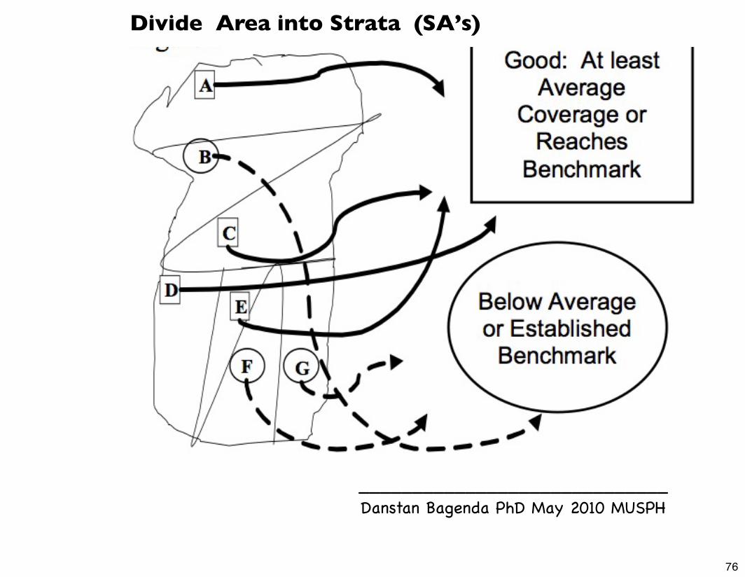
Divide Area into Strata (SA’s)
76
What are the LQAS Principles?
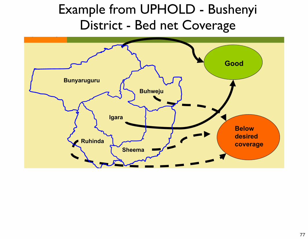
Good
Below desired coverage
Bunyaruguru
RuhindaSheema
Igara
Buhweju
Example from UPHOLD - Bushenyi District - Bed net Coverage
77

_____________________________Danstan Bagenda PhD May 2010 MUSPH
LQAS in Hypothesis terms
• d=no of unimmunized out of sample of n
• Let Q=threshold value or proportion of unimmunized in the population
• Null Hypothesis, Ho: Q≥.50
• (ie popn not adequately immunized)
• Vs Alternative Ha: Q < .50
• (popn adequately immunized)
78
_____________________________Danstan Bagenda PhD May 2010 MUSPH
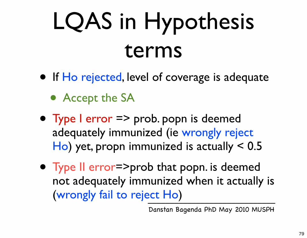
LQAS in Hypothesis terms
• If Ho rejected, level of coverage is adequate
• Accept the SA
• Type I error => prob. popn is deemed adequately immunized (ie wrongly reject Ho) yet, propn immunized is actually < 0.5
• Type II error=>prob that popn. is deemed not adequately immunized when it actually is (wrongly fail to reject Ho)
79

_____________________________Danstan Bagenda PhD May 2010 MUSPH
LQAS in Hypothesis terms
• d=no of unimmunized out of sample of n
• Let Q=threshold value or proportion of unimmunized in the population
• Null Hypothesis, Ho: d≥d*
• (ie popn not adequately immunized)
• Vs Alternative Ha: d<d*
• (popn adequately immunized)
80

_____________________________Danstan Bagenda PhD May 2010 MUSPH
• Choice of d* and n depend upon the desired type I and type II error probabilities
81
_____________________________Danstan Bagenda PhD May 2010 MUSPH
Setting Threshold
• Method CANNOT help manager determine what should be performed or what an adequate or inadequate performance (ie, “Coverage benchmark” means (ie the lower threshold & upper threshold)
• Consensus with stakeholders helps
82
_____________________________Danstan Bagenda PhD May 2010 MUSPH
What you need:
• 3 numbers need to be specified:
• No. “N” of units from SA from which sample is drawn
• No. of units “n” in random sample drawn from SA
• The acceptance no. “d*” - max. allowable no. of “defective units in sample
83
_____________________________Danstan Bagenda PhD May 2010 MUSPH
Decision Rule
• if observed d > d* --- Reject the SA
• Eg:
• With N=50, n=5, & d*=0
• => Take a RS of size 5 from an SA of 50.
• if sample contains > 0 defectives, reject the SA, otherwise accept the SA
84

_____________________________Danstan Bagenda PhD May 2010 MUSPH
Decision Rule testing based on Binomial p
• LQAS uses Binomial Probability to calculate probability of accepting or rejecting an SA
85

_____________________________Danstan Bagenda PhD May 2010 MUSPH
• Vaccination Coverage EG
• Assume coverage of DPT1 for a health area is p
• In health area with infinitely large population, the probability P(a) of selecting a no. a of vaccinated individuals in a sample of size n is calculated as:
• P(a) = nCapaqn-a
86
_____________________________Danstan Bagenda PhD May 2010 MUSPH
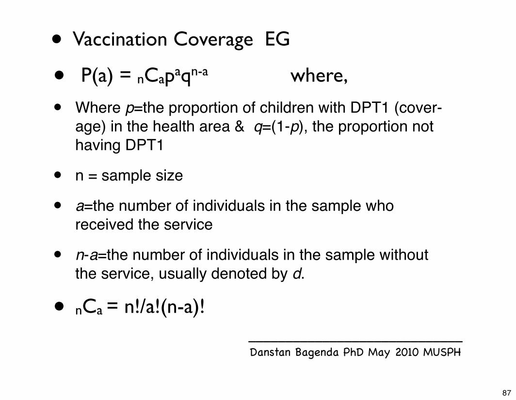
• Vaccination Coverage EG
• P(a) = nCapaqn-a where,
• Where p=the proportion of children with DPT1 (cover-age) in the health area & q=(1-p), the proportion not having DPT1
• n = sample size
• a=the number of individuals in the sample who received the service
• n-a=the number of individuals in the sample without the service, usually denoted by d.
• nCa = n!/a!(n-a)!
87

_____________________________Danstan Bagenda PhD May 2010 MUSPH
But 1st....
• LQAS helps manager choose:
• the sample size
• permissible value of n-a
• interpreting results
88

_____________________________Danstan Bagenda PhD May 2010 MUSPH
But 1st....• 5 decisions need to be made: Select
1. intervention (here DPT1 coverage)
2. program area whose coverage will be assessed
3. target community to receive intervention (eg infants)
4. triage system for classifying coverage as adequate, somewhat inadequate, very inadequate
5. Level of provider & consumer risk: p(wrongly classify provider as unsatisfactory); p(wrongly classify as adequate when inadequate). 10-15%
89
_____________________________Danstan Bagenda PhD May 2010 MUSPH
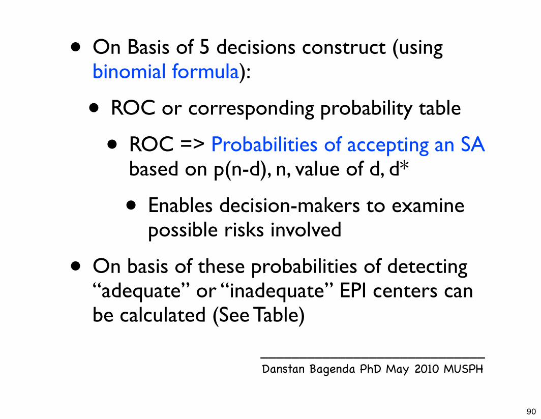
• On Basis of 5 decisions construct (using binomial formula):
• ROC or corresponding probability table
• ROC => Probabilities of accepting an SA based on p(n-d), n, value of d, d*
• Enables decision-makers to examine possible risks involved
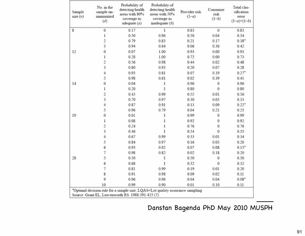
• On basis of these probabilities of detecting “adequate” or “inadequate” EPI centers can be calculated (See Table)
90
_____________________________Danstan Bagenda PhD May 2010 MUSPH
91

_____________________________Danstan Bagenda PhD May 2010 MUSPH
Probabilities in above Table calculated using the binomial formula
The upper & Lower threshold of the triage system were 80% & 50% respectively
Eg.: for n-=12 & d=3
To calculate probability of wrongly classifying provider as inadequate:
1) Calculate probability of having ≤3 unimmunized children - of 12 children in an area with 80% coverage.
2) Subtract this probability from 1 to get the probability of wrongly classifying a provider as inadequate if they may be not inadequate
92

_____________________________Danstan Bagenda PhD May 2010 MUSPH
Probabilities in above Table calculated using the binomial formula
The upper & Lower threshold of the triage system were 80% & 50% respectively
Eg.: for n-=12 & d=3
Therefore, the probability of having three or fewer children unimmunized in an area with 80% coverage is=0.0687+0.2062+0.2835+0.2363=0.7946
93
_____________________________Danstan Bagenda PhD May 2010 MUSPH
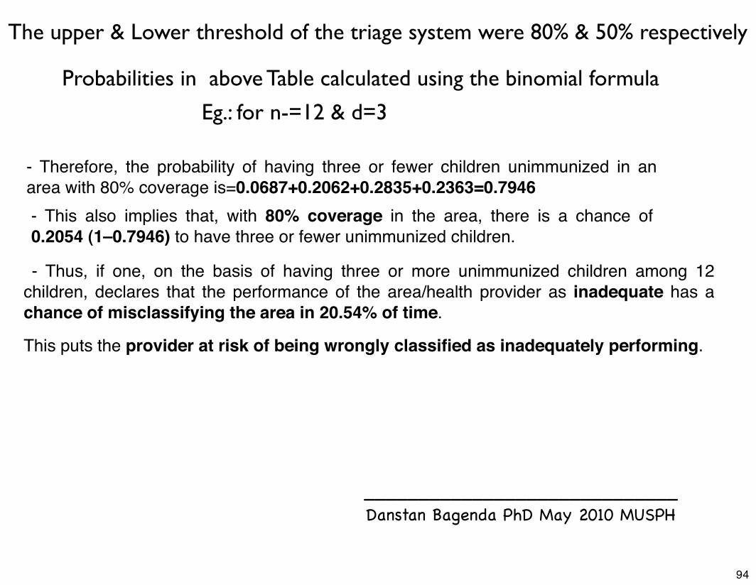
Probabilities in above Table calculated using the binomial formula
The upper & Lower threshold of the triage system were 80% & 50% respectively
Eg.: for n-=12 & d=3
- Therefore, the probability of having three or fewer children unimmunized in an area with 80% coverage is=0.0687+0.2062+0.2835+0.2363=0.7946- This also implies that, with 80% coverage in the area, there is a chance of 0.2054 (1–0.7946) to have three or fewer unimmunized children.
- Thus, if one, on the basis of having three or more unimmunized children among 12 children, declares that the performance of the area/health provider as inadequate has a chance of misclassifying the area in 20.54% of time.
This puts the provider at risk of being wrongly classified as inadequately performing.
94

_____________________________Danstan Bagenda PhD May 2010 MUSPH
Probabilities in above Table calculated using the binomial formula
The upper & Lower threshold of the triage system were 80% & 50% respectively
Eg.: for n-=12 & d=3
- Thus, the decision that an area/health-care provider is performing adequately on the basis of having three or fewer unimmunized children—of 12 children—may, in fact, be wrong in 7.29% of the time.
This puts the community members at risk for they may be considered adequately covered when they are not.
- On the other hand, with 50% coverage, the probability of having three or fewer children unimmunized is=P(12 immunized)+P(11 immunized)+P(10 immunized)+P(9 immunized)=0.0002+0.0029+0.0161+0.0536=0.0729
- This implies that, with 50% coverage, there is still a probability of 0.0729 of having three or fewer unimmunized children.
95
_____________________________Danstan Bagenda PhD May 2010 MUSPH
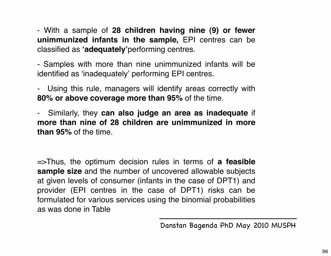
- With a sample of 28 children having nine (9) or fewer unimmunized infants in the sample, EPI centres can be classified as ʻadequatelyʼperforming centres.
- Samples with more than nine unimmunized infants will be identified as ʻinadequatelyʼ performing EPI centres.
- Using this rule, managers will identify areas correctly with 80% or above coverage more than 95% of the time.
- Similarly, they can also judge an area as inadequate if more than nine of 28 children are unimmunized in more than 95% of the time.
=>Thus, the optimum decision rules in terms of a feasible sample size and the number of uncovered allowable subjects at given levels of consumer (infants in the case of DPT1) and provider (EPI centres in the case of DPT1) risks can be formulated for various services using the binomial probabilities as was done in Table
96

_____________________________Danstan Bagenda PhD May 2010 MUSPH
Optimal LQAS Decision Rules for Sample Sizes of 12-24 and Coverage
Benchmarks of 20%-95%
Optimal LQAS Decision Rules for Sample Sizes of 12-24 & Coverage Benchmarks of
20%-95%
97

_____________________________Danstan Bagenda PhD May 2010 MUSPH
EXAMPLE:
98

_____________________________Danstan Bagenda PhD May 2010 MUSPH
Decision Rules for Sample Sizes
99
_____________________________Danstan Bagenda PhD May 2010 MUSPH
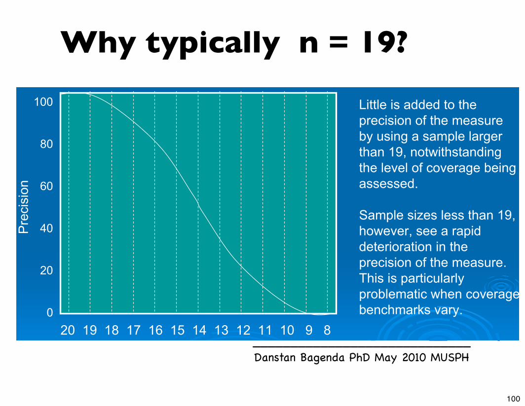
Why 19?Why 19?
20 19 18 17 16 15 14 13 12 11 10 9 8
Pre
cisi
on
100
80
60
40
20
0
Little is added to the precision of the measure by using a sample largerthan 19, notwithstanding the level of coverage being assessed.
Sample sizes less than 19, however, see a rapiddeterioration in the precision of the measure. This is particularly problematic when coveragebenchmarks vary.
Why typically n = 19?
100
_____________________________Danstan Bagenda PhD May 2010 MUSPH
Sample size issues
• For a universe (N) > 500, the properties of binomial distributions are used to compute the sample size (n)
• For a universe (N) < 500, the properties of hypergeometric distributions must be used to compute the sample size (n)
• The larger the N the closer the two methods. For small samples, the hypergeometric distribution is more accurate
101
_____________________________Danstan Bagenda PhD May 2010 MUSPH
Sample size issues
• At least 92% of the time a sample of 19 identifies correctly whether a coverage benchmark has been reached or whether a supervision area is below the average coverage of a program area
• Samples n > 19 have practically the same statistical precision as 19—they do not result in better information and they cost more.
• Samples n< 19 do not produce results exact enough to make good management decisions.
102

_____________________________Danstan Bagenda PhD May 2010 MUSPH
What a sample of 19 can tell you
• Lower performing supervision areas that require action
• Higher performing supervision areas to learn from
• Priorities among supervision areas with large differences
• Indicators that have high coverage
• Indicators that have low coverage
• Priorities within a supervision area (indicators that fall short of the benchmark vs. those that do not)
103
_____________________________Danstan Bagenda PhD May 2010 MUSPH
What a sample of 19 cannot tell you
• Exact coverage in an SA (but can be used to calculate coverage for an entire program)
• Priorities among supervision areas with little difference in coverage
104
_____________________________Danstan Bagenda PhD May 2010 MUSPH
Limitations of LQAS• Only allows to tell whether a lot « passes » or
« fails » on a pre-defined criteria
• Because the sample size is so reduced
• The creation of sub groups and stratified analyses is impossible ; and
• Any reduction in the size of the sample (e.g. due to attrition or loss of cases) threatens its representativeness and makes the analysis more complex
105
_____________________________Danstan Bagenda PhD May 2010 MUSPH
What this means..• Low sample size needs (n=19 in most
cases
• Simple to apply yet very specific conclusions
• Result=High quality information at low costs
• BUT
• Only dichotomous outcomes allowed(pass/fail, complies/not complies, yes/no)
• Subsets are problematic
106

_____________________________Danstan Bagenda PhD May 2010 MUSPH
Resources• http://danstan.com/blog/imHotep/
http://faculty.vassar.edu/lowry/VassarStats.html
107

_____________________________Danstan Bagenda PhD Nov 2009 MUSPH
End
108

_____________________________Danstan Bagenda PhD Nov 2009 MUSPH
Exercise
1) What is the decision threshold
d* based on benchmark?
2) Which SA’s are below benchmark
& warrant intervention?
(Note: Use Decision Table page 99)
109


