
Statistical Classification Rong Jin. Classification Problems X Input Y Output ? Given input X={x 1,...
45
Statistical Classification Rong Jin
-
Upload
judith-tucker -
Category
Documents
-
view
237 -
download
1
Transcript of Statistical Classification Rong Jin. Classification Problems X Input Y Output ? Given input X={x 1,...

Statistical Classification
Rong Jin

Classification ProblemsYXf :
XInput Y Output?
• Given input X={x1, x2, …, xm}
• Predict the class label y Y
• Y = {-1,1}, binary class classification problems
• Y = {1, 2, 3, …, c}, multiple class classification problems
• Goal: need to learn the function: f: X Y

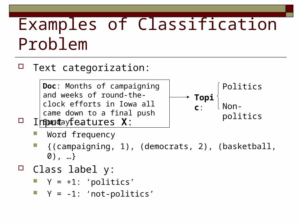
Examples of Classification Problem Text categorization:
Input features X: Word frequency {(campaigning, 1), (democrats, 2), (basketball, 0), …}
Class label y: Y = +1: ‘politics’ Y = -1: ‘non-politics’
Doc: Months of campaigning and weeks of round-the-clock efforts in Iowa all came down to a final push Sunday, …
Topic:
Politics
Non-politics
Examples of Classification Problem Text categorization:
Input features X: Word frequency {(campaigning, 1), (democrats, 2), (basketball, 0), …}
Class label y: Y = +1: ‘politics’ Y = -1: ‘not-politics’
Doc: Months of campaigning and weeks of round-the-clock efforts in Iowa all came down to a final push Sunday, …
Topic:
Politics
Non-politics

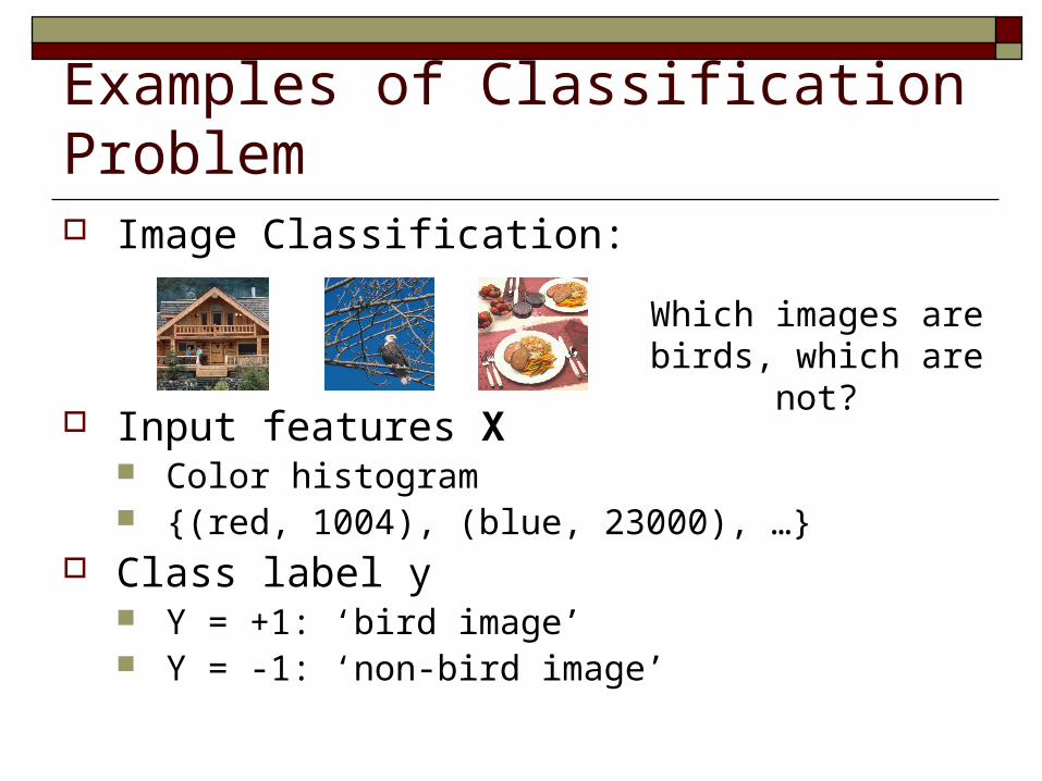
Examples of Classification Problem Image Classification:
Input features X Color histogram {(red, 1004), (red, 23000), …}
Class label y Y = +1: ‘bird image’ Y = -1: ‘non-bird image’
Which images are birds, which are not?
Examples of Classification Problem Image Classification:
Input features X Color histogram {(red, 1004), (blue, 23000), …}
Class label y Y = +1: ‘bird image’ Y = -1: ‘non-bird image’
Which images are birds, which are not?

Classification ProblemsYXf :
XInput Y Output?
Doc: Months of campaigning and weeks of round-the-clock efforts in Iowa all came down to a final push Sunday, …
Politics Not-politics
f: doc topic
Birds Not-Birds
f: image topicHow to obtain f ?
Learn classification function f from examples

Learning from Examples Training examples:
Identical Independent Distribution (i.i.d.) Each training example is drawn independently from the identical source Training examples are similar to testing examples
1 1 2 2
,1 ,2 ,
, , , ,..., ,
: the number of training examples
: , ,...,
:
Binary class: { 1, -1}
Multiple class: {1,2,..., }
train n n
di i i i d
i
D x y x y x y
n
x x x x
y
c
Y
Y
Y

Learning from Examples Training examples:
Identical Independent Distribution (i.i.d.) Each training example is drawn independently from the identical source
1 1 2 2
,1 ,2 ,
, , , ,..., ,
: the number of training examples
: , ,...,
:
Binary class: { 1, -1}
Multiple class: {1,2,..., }
train n n
di i i i d
i
D x y x y x y
n
x x x x
y
c
Y
Y
Y

Learning from Examples Given training examples
Goal: learn a classification function f(x):XY that is consistent with training examples
What is the easiest way to do it ?
1 1 2 2, , , ,..., ,train n nD x y x y x y

K Nearest Neighbor (kNN) Approach
(k=1)(k=4)
How many neighbors should we count ?

Cross Validation Divide training examples into two sets
A training set (80%) and a validation set (20%) Predict the class labels of the examples in the
validation set by the examples in the training set
Choose the number of neighbors k that maximizes the classification accuracy

Leave-One-Out Method
For k = 1, 2, …, K
Err(k) = 0;
1. Randomly select a training data point and hide its class label
2. Using the remaining data and given K to predict the class label for the left data point
3. Err(k) = Err(k) + 1 if the predicted label is different from the true label
Repeat the procedure until all training examples are tested
Choose the k whose Err(k) is minimal
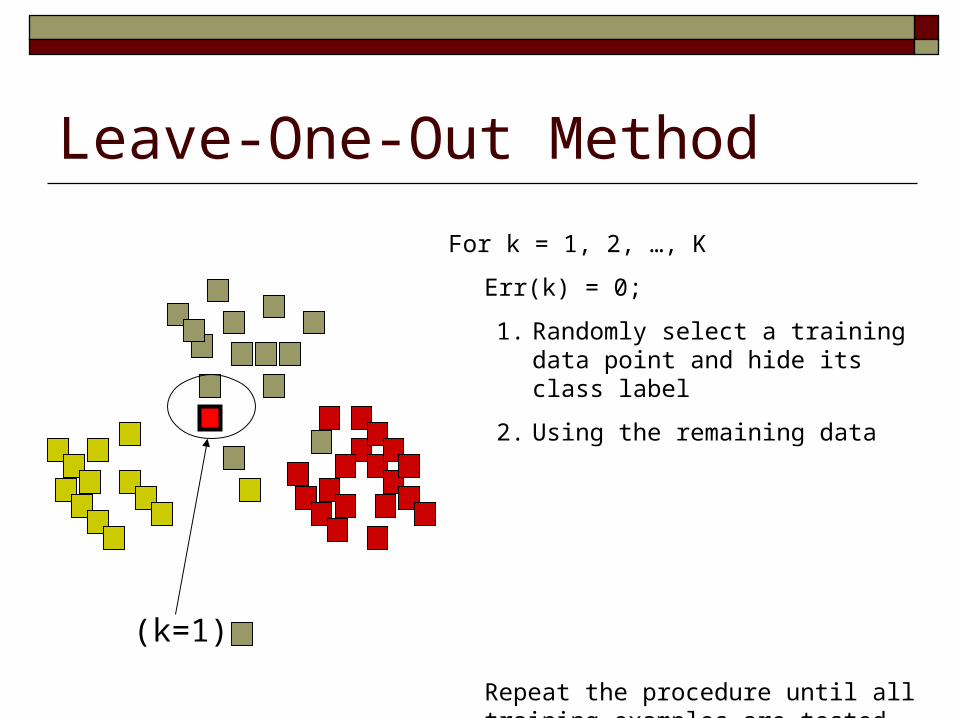
Leave-One-Out Method
For k = 1, 2, …, K
Err(k) = 0;
1. Randomly select a training data point and hide its class label
2. Using the remaining data and given k to predict the class label for the left data point
3. Err(k) = Err(k) + 1 if the predicted label is different from the true label
Repeat the procedure until all training examples are tested
Choose the k whose Err(k) is minimal(k=1)

Leave-One-Out Method
For k = 1, 2, …, K
Err(k) = 0;
1. Randomly select a training data point and hide its class label
2. Using the remaining data and given k to predict the class label for the left data point
3. Err(k) = Err(k) + 1 if the predicted label is different from the true label
Repeat the procedure until all training examples are tested
Choose the k whose Err(k) is minimal(k=1) Err(1) = 1
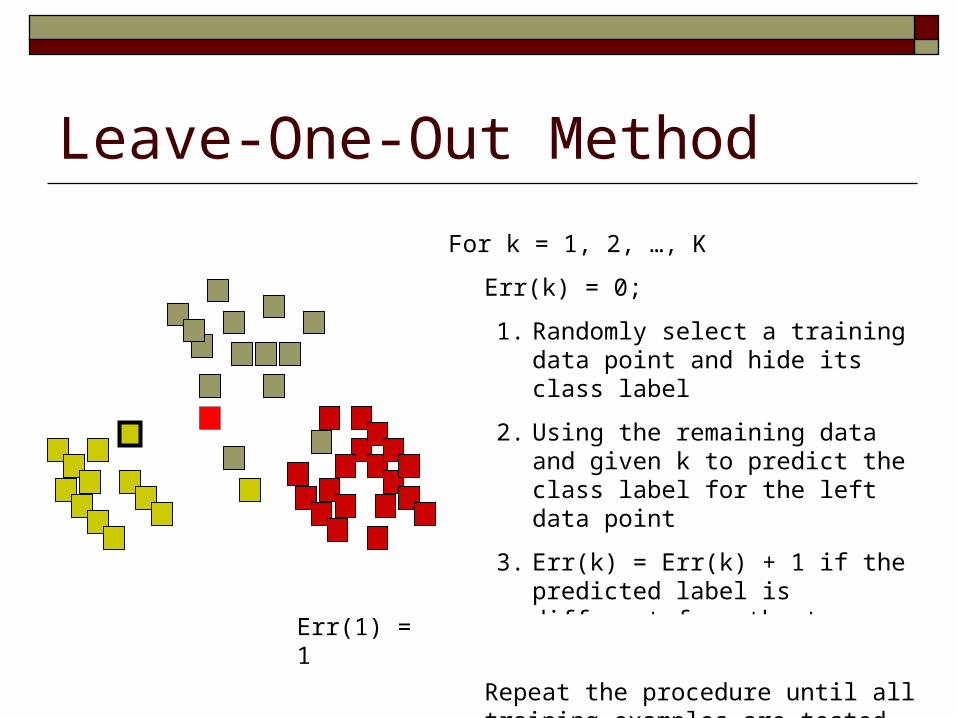
Leave-One-Out Method
For k = 1, 2, …, K
Err(k) = 0;
1. Randomly select a training data point and hide its class label
2. Using the remaining data and given k to predict the class label for the left data point
3. Err(k) = Err(k) + 1 if the predicted label is different from the true label
Repeat the procedure until all training examples are tested
Choose the k whose Err(k) is minimalErr(1) = 1

Leave-One-Out Method
For k = 1, 2, …, K
Err(k) = 0;
1. Randomly select a training data point and hide its class label
2. Using the remaining data and given k to predict the class label for the left data point
3. Err(k) = Err(k) + 1 if the predicted label is different from the true label
Repeat the procedure until all training examples are tested
Choose the k whose Err(k) is minimal
Err(1) = 3
Err(2) = 2
Err(3) = 6
k = 2

Probabilistic interpretation of KNN Estimate the probability density function Pr(y|x)
around the location of x Count of data points in class y in the neighborhood of x
Bias and variance tradeoff A small neighborhood large variance unreliable
estimation A large neighborhood large bias inaccurate
estimation

Weighted kNN Weight the contribution of each close neighbor
based on their distances Weight function
Prediction
2
2
2
2exp),(
i
i
xxxxw
i i
ii i
xxw
yyxxwxy
),(
),(),()|Pr(
i
ii yy
yyyy
0
1),(

Estimate 2 in the Weight Function Leave one cross validation Training dataset D is divided into two sets
Validation set Training set
Compute the
),( 11 yx
),(),...,,(),,( 33221 nn yxyxyxD
),|Pr( 111 Dxy

Estimate 2 in the Weight Function
n
i
i
i
n
i
i
n
ii
i
n
ii
xx
yyxx
xxw
yyxxwDxy
22
2
21
12
2
2
21
21
12
1
111
2exp
),(2
exp
),(
),(),(),|Pr(
Pr(y|x1, D-1) is a function of 2

Estimate 2 in the Weight Function
n
i
i
i
n
i
i
n
ii
i
n
ii
xx
yyxx
xxw
yyxxwDxy
22
2
21
12
2
2
21
21
12
1
111
2exp
),(2
exp
),(
),(),(),|Pr(
Pr(y|x1, D-1) is a function of 2

Estimate 2 in the Weight Function In general, we can have expression for
Validation set Training set
Estimate 2 by maximizing the likelihood
),|Pr( iii Dxy
),( ii yx
),()...,,(),,(),....,,( 111121 nniiiii yxyxyxyxD
n
iiii Dxyl
1
),|Pr(log
)(maxarg*
l

Estimate 2 in the Weight Function In general, we can have expression for
Validation set Training set
Estimate 2 by maximizing the likelihood
),|Pr( iii Dxy
),( ii yx
),()...,,(),,(),....,,( 111121 nniiiii yxyxyxyxD
n
iiii Dxyl
1
),|Pr(log
)(maxarg*
l

Optimization
n
i
ik
ki
ikik
ki
n
iiii
xx
yyxx
Dxyl1
2
2
2
2
2
2
1
2exp
),(2
exp
log),|Pr(log
)(maxarg*
l
It is a DC (difference of two convex functions) function

Challenges in Optimization Convex functions are easiest to be optimized Single-mode functions are the second easiest Multi-mode functions are difficult to be optimized

Gradient Ascent
n
i
ik
ki
ikik
ki
n
iiii
xx
yyxx
Dxyl1
2
2
2
2
2
2
1
2exp
),(2
exp
log),|Pr(log
2
2
21 1 2
exp ( , )
log Pr( | , ) logexp
i k k in nk i
i i ii i i k
k i
x x y y
l y x Dx x
21/

Gradient Ascent (cont’d)
Compute the derivative of l(λ), i.e., Update λ
2
2
21 1 2
exp ( , )
log Pr( | , ) logexp
i k k in nk i
i i ii i i k
k i
x x y y
l y x Dx x
( ) /dl d
( )dlt
d
How to decide the step size t?

Gradient Ascent: Line Search
Excerpt from the slides by Steven Boyd

Gradient Ascent Stop criterion
is predefined small value
Start λ=0, Define , , and Compute Choose step size t via backtracking line search Update Repeat till
| ( ) / |dl d
( ) /dl d
( ) /tdl d | ( ) / |dl d

Gradient Ascent Stop criterion
is predefined small value
Start λ=0, Define , , and Compute Choose step size t via backtracking line search Update Repeat till
| ( ) / |dl d
( ) /dl d
( ) /tdl d | ( ) / |dl d

ML = Statistics + Optimization Modeling Pr(y|x;)
is the parameter(s) involved in the model Search for the best parameter
Maximum likelihood estimation Construct a log-likelihood function l() Search for the optimal solution

Instance-Based Learning (Ch. 8) Key idea: just store all training examples k Nearest neighbor:
Given query example , take vote among its k nearest neighbors (if discrete-valued target function)
take mean of f values of k nearest neighbors if real-valued target function
qx

When to Consider Nearest Neighbor ? Lots of training data Less than 20 attributes per example Advantages:
Training is very fast Learn complex target functions Don’t lose information
Disadvantages: Slow at query time Easily fooled by irrelevant attributes

KD Tree for NN Search
Each node contains Children information The tightest box that bounds all the data points within the node.

NN Search by KD Tree

NN Search by KD Tree

NN Search by KD Tree

NN Search by KD Tree

NN Search by KD Tree

NN Search by KD Tree

NN Search by KD Tree

Curse of Dimensionality Imagine instances described by 20 attributes, but only 2 are
relevant to target function Curse of dimensionality: nearest neighbor is easily mislead
when high dimensional X Consider N data points uniformly distributed in a p-
dimensional unit ball centered at original. Consider the nn estimate at the original. The mean distance from the original to the closest data point is:
1/1( , ) 1 2
pNd p N

Curse of Dimensionality Imagine instances described by 20 attributes, but only 2 are
relevant to target function Curse of dimensionality: nearest neighbor is easily mislead
when high dimensional X Consider N data points uniformly distributed in a p-
dimensional unit ball centered at origin. Consider the nn estimate at the original. The mean distance from the origin to the closest data point is:
p
NNpd
pN log121),(
/1/1


