Statistical Asymmetry-based Brain TumorSegmentation from 3D MR Images

Chen-Ping Yu1, Guilherme C. S. Ruppert23, Dan T. D. Nguyen4,Alexandre X. Falcao2, and Yanxi Liu1

1 Department of Computer Science and Engineering, Pennsylvania State University,342 Information Sc. and Tech. Building, University Park, PA, USA 16802

cpu1982@gmail.com,yanxi@cse.psu.edu2 Institute of Computing, University of Campinas, Av. Albert Einstein 1251,

Campinas, Brazil 13083-852{ruppert,afalcao}@ic.unicamp.br

3 Renato Archer Center for Information Technology, Rod. Dom Pedro km143,Campinas, Brazil 13069-901

guilherme.ruppert@cti.gov.br4 Department of Radiology, Penn State Hershey Medical Center, 500 University Drive,

Hershey, PA, USA 17033dnguyen1@hmc.psu.edu

Abstract. The precise segmentation of brain tumors from MR images is nec-essary for surgical planning. However, it is a tedious task for the medical pro-fessionals to process manually. The performance of supervised machine learningtechniques for automatic tumor segmentation is time consuming and very depen-dent on the type of the training samples. Brain tumors are statistically asymmetri-cal blobs with respect to the mid-sagittal plane (MSP) in the brain and we presentan asymmetry-based, novel, fast, fully-automatic and unsupervised frameworkfor 3D brain tumor segmentation from MR images. Our approach detects asym-metrical intensity deviation of brain tissues in 4 stages: (1) automatic MSP ex-traction, (2) asymmetrical slice extraction for an estimated tumor location, (3)region of interest localization, and (4) 3D tumor volume delineation using a wa-tershed method. The method has been validated on 17 clinical MR volumes witha 71.23%±27.68% mean Jaccard Coefficient.

1 Introduction

Brain tumors vary in size, shape, color, and location, which is precisely the reason whyautomatic tumor segmentation is challenging. While the medical professionals are ableto hand label the optimal details of each tumor case, such task is incredibly tedious andtime-consuming. Therefore, the need for tumors to be automatically segmented remainsan unsolved problem in clinical practice.

In recent years, related unsupervised approaches that utilizes brain asymmetry [22][9] requires human interaction to manually select a 2D slice of interest, and the 2D/3Dtumor segmentation from such analysis has not been shown to work fully automatically.

Markov Random Fields [15] and Conditional Random Field [12] based machinelearning techniques have been applied in tumor segmentation tasks as well. Meth-ods like Discriminative Random Fields [11], Support Vector Random Fields [13], and

Fig. 1. Sample result for case 6, showing the 3 orientations and the 3D view on the lower rightportion of the figure, with Jaccard Coefficient of 90.11%.

Pseudo-Conditional Random Field [14] have been shown to offer better performance.Other supervised statistical machine learning approaches include using fractal features[8], alignment features [23], one-class support vector machine [26], using Bayesianclassifier [5], tumor localization using diagonal nearest-neighbors [7], segmentationby outliers [21], and high-dimensional features with level-set [3]. A recent supervisedmethod proposed [27], though demonstrating promising results on small tumor detec-tion using brain asymmetry, is not addressing 3D tumor segmentation problem.

In order to extract features to be used for pixel/voxel classification, standard ma-chine learning methods must first register the input volume. The registration processusually takes hours of time while being a research area of its own [10]; the performanceaccuracy of the classification and segmentation result depends largely on the trainingsamples and the pre-defined feature sets.

Unsupervised algorithms using the bilateral symmetry of the brain start to emergein recent years [16][22]. However, unsupervised methods based on symmetry are stillin its early stages as such methods are not yet fully automatic, and the accuracy also hasa lot of room for improvements [16][22].

In this paper, we present a novel, fully automatic and unsupervised framework thatis based upon an intuitive yet statistically justified observation that tumors are one of themost prominent asymmetrical blobs in the brain. We show that our approach is invariantto different types of tumor with the asymmetrical blob assumption, and we are able toautomatically localize and delineate the tumors. The entire process is fast due to theunsupervised nature, taking about 3 minutes to run.

2 Statistical Asymmetry-based Method

Human brains are commonly accepted as statistically symmetrical with respect to itsMid-Sagittal Plane (MSP)[24]. Our proposed method takes the advantage of this prop-

Fig. 2. Diagram of the entire process of the proposed 4-stage algorithm.

Fig. 3. Examples of results from Stage 1 (MSP extraction). The Figure shows 4 pairs (originalimage and the results from the method) for cases 1, 3, 4 and 10 with slice 184, 160, 161, and 156respectively.

erty by processing the brain through asymmetry comparisons of its structural and pixelintensity distribution. We propose a 4-stage process: 1) MSP alignment, 2) locate an ax-ial slice that contains parts of the tumor, 3) localize the 2D shape of the tumor from theextracted slice-of-interest (SOI), 4) grow the 3D shape of the tumor out bi-directionally.

2.1 Stage 1: Automatic Mid-Saggital Plane Extraction

Since this work is a symmetry-based method, it depends on the bi-lateral symmetryanalysis of the brain, which requires the localization of the mid-sagittal plane (MSP)which is the reference of symmetry of the brain. Based on the MSP location, the imagecan be realigned, i.e. rotated and translated in a way so the MSP is found in the centralslice of the image. In order to perform the MSP extraction, first, all input images werere-interpolated to isotropic voxels to restore the original proportion of the brain.

The method described in [24] was used to automatically locate the mid-sagittalplane (MSP). It is a very fast and accurate method for MSP extraction and is basedon bi-lateral symmetry maximization. It uses cross-correlation of edges in the full 3Ddomain as the symmetry criteria and finds the plane that maximizes this criteria usingan optimized multi-scale search algorithm. On average, the method takes less than 25sto run on a modern desktop machine over a typical MRI data. Figure 3 shows someexamples of the results from this method.

2.2 Stage 2: Slice of Interest (SOI) Extraction

We formulate the problem using a Bayesian model,

P (Z|SZ) ∝ P (SZ |Z)× P (Z) (1)

Our goal is to extract a 2D slice E[S] from the volume of interest (VOI) that con-tains part of the tumor, where we obtainE[S] from the posterior P (Z|SZ) by maximiz-ing the conditional likelihood P (SZ |Z). We define SZ as the full count of axial-viewslices from the neck towards the top of the head, where SZ = { SL|Z , SR|Z | Z =1, ..., z, L = l1, ..., lu, R = r1, ..., ru}, and a prior P (Z) that models the likelihood oftumor location.

The brain is split into 2 halves along MSP of SZ , where SL|Z and SR|Z are the leftand right half. SL|Z and SR|Z are then further equally partitioned perpendicular to theMSP into u pieces for the consideration of spatial information.

We compute an asymmetry score using Earth-Mover Distance [17] for each pair ofSL|Z and SR|Z that is equally partitioned into u pieces. The Earth-Mover Distance be-tween two normalized histogramsH(A) andH(B) is denoted here asΦ(H(A), H(B) ).The normalized 3-dimensional histogram (x,y location and the intensity level at eachpixel) of each partitioned piece are denoted asH3(Slu|Z) andH3(Sru|Z). To determinehow asymmetrically distributed are the intensity values of Sz with its piece-wise spatialinformation, each pair of partitions’ EMD asymmetry scores are summed to form thelikelihood probability:

P (SZ) =

u∑i=1

Φ( H3(Slu|Z), H3(Sru|Z) ) (2)

We obtain the likelihood probability from each slice Sz , which we can plot and treatas a 1D signal (Figure 4). We wish to locate the most asymmetrical slice. However, thissignal can be noisy due to different parts of the brain (especially the neck region and thescalp top) and intensity variance, therefore we must apply a prior P (Z) that models thelikelihood of tumor location. We found that parts of the Inverse-Gamma distributionresembles the prior likelihood of tumor location well (Figure 4). We denote Inverse-Gamma as f(Z;α, β), and it is defined as:

P (Z) = f(Z;α, β) =βα

Γ (α)(1/Z)α+1e−β/Z (3)

The Inverse-Gamma prior formulates the likelihood P (SZ) into a conditional prob-ability P (SZ |Z). Now we can calculate Bayesian posterior probability P (Z|SZ) fromthe originally obtained conditional likelihood signal P (SZ |Z) with the Inverse-Gammaprior P (Z).

After P (Z|SZ) is computed, any posterior probability that is outside of 3σ is re-duced to the mean of the entire posterior probability and its SZ−2, SZ−1, SZ+1, andSZ+2 neighbors as a measure to remove outliers. The processed posterior probabilityP (Z|SZ) is convoluted by 1D Gaussian filter N(µ = 0, σ2 = 3) with horizontal sizeof 9 (spans 4 slices before and after the current position) for all observations to beweighted by their neighboring information as well as filtering out the high frequency

Fig. 4. The complete process of Slice of InterestE[S] extraction: (a) Inverse-Gamma prior P (Z),(b) spatially-constrained EMD asymmetry distance for SZ , (c) posterior probability P (Z|SZ),(d) P (Z|SZ) is filtered by Gaussian low-pass filter with σ = 3, (e) the most asymmetrical sliceE[S] extracted as the maxima of P (Z|SZ).

Fig. 5. Case #1 intermediate results for tumor blob detection: (a) E[S], (b) extracted CSDD blob

features→B, (c) the top 5% most asymmetrical blobs

→B∗ the whiter the outline represents the

higher asymmetrical score, with the extracted MSP as the white vertical line, (d) result of k-means clustering with y-axis as the tumor-likelihood P (B∗j ) for each blob B∗j , (e) retaining the

cluster that yields the higher mean P (B∗j ) gives us the true positive tumor blobs E[→B∗], (f) the

final 2D rough tumor shape.

noises (Figure 4). Finally we can take the maxima of this signal to be our E[S] andproceed to segment tumor’s 2D shape (Figure 4). We define the convulotion of f and gas f ? g, and by setting the parameters Z = 1 : z, µ = 0, and σ = 3, we are able to findthe tumor slice:

E[S] = max{ P (Z|SZ) ? N(µ, σ) } (4)

2.3 Stage 3: Blob Feature Extraction with Asymmetry Processing

From the extracted slice of interest, we proceed to extract the tumor’s 2D shape with astate of the art blob detector. We use Center-Surround Distribution Distance (CSDD) [4]as our blob and interest region detector, which is insensitive to geometric deformation.CSDD is based on comparing the cumulative distributions of intensity and texture of anextracted region and its surrounding circular background.

E[S] is first smoothed with Gaussian low-pass filter, where N(l = 5, µ = 0, σ2 =2) to get rid of possible noise, then CSDD blob features [4] are extracted from the fil-

tered E[S] (Figure 5). We denote the extracted blob features as→B with each single blob

feature denoted as Bi. To eliminate all the false positives blobs that do not surround theactual tumor, we compute the EMD [17] of the intensity distribution 1D histogram (onlyintensity information) from the areas enclosed by each blob Bi and its corresponding

MSP-reflection areaRef(Bi), and retain the highest 5% EMD metric blobs, denoted as→B∗, in which blobs with higher EMD score imply the enclosed structure as being moreasymmetrical.

→B∗= max{ Φ( H1(Bi), H1(Ref(Bi)) ),

⌊5N

100

⌋} (5)

We define and compute the tumor-likelihood score P (B∗j ) of each blobs B∗j of→B∗ by weighting EMD asymmetry score of B∗j with its blob strength S(B∗j ), whichis the EMD measure of how distinctive is the foreground and background intensity ofblob B∗j . Then, we dividing the weighted asymmetry score by its foreground intensityvariance V ar[I(B∗j )], because the non-tumor false positives such as part of the scalpand surrounding tissues may yield high intensity variance, whereas the tumor tissue inan area remains uniform intensity.

P (B∗j ) =S(B∗j ) Φ( H1(B

∗j ), H1( Ref(B

∗j ) ) )

V ar[ I(B∗j ) ](6)

K-means clustering [2] algorithm with k = 2 is then used to cluster P (→B∗) into

two groups→B∗k=1 and

→B∗k=2, and the expected tumor blobs E[

→B∗] can be retained by

keeping the cluster that yields the highest likelihood (Figure 5).

E[→B∗] = max{ avg(

→B∗k=1), avg(

→B∗k=2) } (7)

It is possible that E[→B∗] can have blobs at spur and false positive locations instead

of one connected component. In which case, we use a heuristic approach to removeoutlier blobs by keeping the connected component that has the most blobs with thehighest EMD asymmetry score Φ(H1(B

∗j ), H1( Ref(B

∗j ) ). To obtain the final rough

2D location and shape of the tumor from E[→B∗], simply segment the combined contour

of the blobs E[→B∗], which yields the rough 2D shape of the tumor (Figure 5).

2.4 Stage 4: 3D Tumor Delineation by IFT (image forest transform) Watershed

The previous steps provide the approximate location of the tumor and a rough shape ofthis tumor within the SOI. The next step is the precise delineation of the tumor and thisis performed for the whole 3D image.

The approach we use in this work utilizes markers-controlled watershed, placing ob-ject and background seeds within the SOI and letting the watershed grow the regions in3D. However, there are many different algorithms of watershed and their segmentationresults are not the same [1]. In this work, we use the IFT-watershed [18] which is basedon the Image Foresting Transform [18]. IFT is a general tool for designing of imageprocessing operators based on connectivity, reducing image processing problems intoan optimum path forest problem in a graph derived from the image. We chose the IFT-watershed method because it is considerably faster [18] and implements the watershed

Fig. 6. IFT-Watershed segmentation process and result. (a) input image, (b) initial mask, (c) tumorseeds, (d) background seeds, (e)-(f) final segmentation in axial, coronal and sagittal orientation,respectively.

in such a way that resolves the ”tie zones” dividing them in a balanced manner betweenthe seeds. Further information about the details and evaluation of the IFT-Watershedcan be found in [1] and [18].

However, the watershed requires an initialization by placing some object and back-ground seeds, so we developed a way to automatically place these seeds using the resultfrom the blobs extraction stage. In our case, the term ”object” below refers to the tumor,and the background refers to everything else.

The result from the blob extraction is a 2D binary mask (where we have zero forbackground and one for object). To generate the object seeds, we apply the erosionmorphological operator on this mask using a circular structuring element with radiusadaptive to the input mask. This morphological operation is performed in 2D within theSOI. The result is shown in Table 6. The background seeds are generated in a similarway by applying the dilation operator instead of erosion but then computing the com-plement of the image (inverting values 0 for 1 and vice-versa), resulting in the imageshown in Table 6.

In essence, we create a region of uncertainty around the borders of the mask withinthe SOI. By definition, the internal seed voxels are already considered to be tumorvoxels, and the background seeds are non-tumor voxels. The unmarked voxels are theregion of uncertainty which will be resolved by the IFT-Watershed.

Although the seed generation is performed only in one slice (SOI), we let the water-shed grow to the rest of the 3D image. Figure 6 shows the resulting segmentation afterthe IFT-Watershed.

3 Results

We test our algorithm on 17 MRI data. The 17 3D MR volumes are T1 weighted andpost gadolinium enhanced images acquired in the Axial plane. Other modalities such asT2 or FLAIR are not required by our proposed method.

By visual inspection, the MSP alignments (stage 1) are sucessful for all 17 brainscans in the dataset,which is critical to the success of our symmetry based algorithm.Stage 2 (SOI extraction) located correct slices for 14 out of 17 cases, where stage 3 (2Dlocalization) located the correct tumor location in 13 of 14. Stage 4 (IFT-Watershed)was able to segment the 3D shape of the tumor in all 13 with 1 of which that was not as

Fig. 7. Sample Results. Row 1 to 3: Case 5, 6, and 11.

good due to complicated tumor tissue. Overall, our stage 3 and stage 4 generates veryrobust results based on the slice that was extracted from stage 2.

Quantitative results are calculated using Jaccard Coefficient, where the True Posi-tives (TP) are identified as the overlap between the manually segmented ground truthtumor labels and the machine generated tumor labels.

Jaccard Coefficient:

JC =TP

FP + FN + TP(8)

Our proposed algorithm achieves the mean Jaccard Coefficient of 71.23%±27.68%and the median of 81.68% from the cases that produced outputs. If we disregard case 17where it failed miserably and should be considered as a failure case, our mean JaccardCoefficient is in fact 77.11%± 18.57%. We also visually inspect the output of each in-termediate stages and label the result as either Match and Mismatch to indicate whetheror not the tumor has been located. To further demonstrate the robustness of the bloblocalization (stage 3) asymmetry processing, we manually select a tumor slice if stage2 fails to locate a tumor slice (case 10, 12, and 15) and shows very high accuracy. Table2 shows the complete quantitative results where bold letters indicate manual selectedtumor slice in the case of failed stage 2.

Comparing to other unsupervised and symmetry-based methods [16][22], our pro-posed method is able to work fully automatically without any user intervention, and isprocessed fully in 3D. We also achieve a much higher accuracy than what’s reportedfrom [22] (highest segmentation score being 71.15%), with very fast mean run time ofunder 3 minutes per 3D MR scan, which is very fast comparing to recent publicationsin both supervised and unsupervised related work.

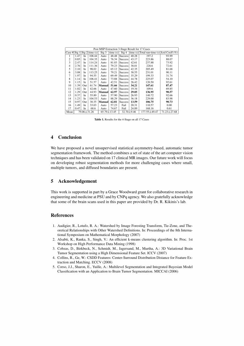
Post MSP Extraction 3-Stage Result for 17 CasesCase # Stg 1 Stg 2 time (s) Stg 3 time (s) Stg 4 time (s) Total run-time (s) Jcrd Coeff (%)

1 1.47 In 108.44 Auto 48.48 Success 40.28 197.2 93.992 0.85 In 104.35 Auto 76.34 Success 43.17 223.86 88.073 2.47 In 114.24 Auto 81.03 Success 42.61 237.88 73.924 2.76 In 111.36 Auto 79.23 Success 38.01 228.6 72.615 2.10 In 98.02 Auto 65.12 Success 42.35 205.49 81.686 3.08 In 113.25 Auto 79.21 Success 38.55 231.01 90.117 1.97 In 94.55 Auto 69.49 Success 35.29 199.33 31.748 1.14 In 106.41 Auto 73.88 Success 44.78 225.07 54.109 1.15 In 51.57 Auto 42.51 Success 26.42 120.50 92.6110 1.39 Out 61.74 Manual 51.66 Success 34.21 147.61 87.4711 1.02 In 42.66 Auto 47.60 Success 19.34 109.6 69.8512 1.29 Out 44.93 Manual 62.97 Success 29.05 136.95 90.5713 0.37 In 55.89 Auto 57.90 Success 26.93 140.72 92.6614 1.23 In 104.53 Auto 88.29 Success 36.18 229.00 83.9815 0.97 Out 30.35 Manual 62.81 Success 13.59 106.75 90.7316 1.49 In 33.03 Auto 57.23 Fail 20.31 110.57 0.0017 0.47 In 68.6 Auto 74.67 Fail 24.89 168.16 0.61

Mean 79.06±31.26 65.79±13.45 32.70±9.46 177.55±49.47 71.23±27.68

Table 1. Results for the 4-Stage on all 17 Cases

4 Conclusion

We have proposed a novel unsupervised statistical asymmetry-based, automatic tumorsegmentation framework. The method combines a set of state of the art computer visiontechniques and has been validated on 17 clinical MR images. Our future work will focuson developing robust segmentation methods for more challenging cases where small,multiple tumors, and diffused boundaries are present.

5 Acknowledgement

This work is supported in part by a Grace Woodward grant for collaborative research inengineering and medicine at PSU and by CNPq agency. We also gratefully acknowledgethat some of the brain scans used in this paper are provided by Dr. R. Kikinis’s lab.

References

1. Audigier, R., Lotufo, R. A.: Watershed by Image Foresting Transform, Tie-Zone, and The-oretical Relationships with Other Watershed Definitions. In: Proceedings of the 8th Interna-tional Symposium on Mathematical Morphology (2007)

2. Alsabti, K., Ranka, S., Singh, V.: An efficient k-means clustering algorithm. In: Proc. 1stWorkshop on High Performance Data Mining (1998)

3. Cobzas, D., Birkbeck, N., Schmidt, M., Jagersand, M., Murtha, A.: 3D Variational BrainTumor Segmentation using a High Dimensional Feature Set. ICCV (2007)

4. Collins, R., Ge, W.: CSDD Features: Center-Surround Distribution Distance for Feature Ex-traction and Matching. ECCV (2008)

5. Corso, J.J., Sharon, E., Yuille, A.: Multilevel Segmentation and Integrated Bayesian ModelClassification with an Application to Brain Tumor Segmentation. MICCAI (2006)

6. Bergo, F.P., Falcao, A., Yasuda, C., Ruppert, G.: FAST AND ROBUST MID-SAGITTALPLANE LOCATION IN 3D MR IMAGES OF THE BRAIN: Biomedical Engineering Sys-tems and Technologies, vol. 25, pp. 278-290 (2008)

7. Gering, D.T.: Diagonalized nearest neighbor pattern matching for brain tumor segmentation.MICCAI (2003)

8. Iftekharuddin, K.M., Zheng, J., Islam, M.A., Ogg, R.J.: Fractal-based brain tumor detectionin multimodal MRI. AMC (2008)

9. Joshi, S., Lorenzen, P., Gerig, G., Bullitt, E.:Structural and radiometric asymmetry in brainimages. Medical Image Analysis, 7(2): 155-170 (2003)

10. Klein, A., Andersson, J., Ardekani B.A., Ashburner J., Avants B., Chiang M.C., ChristensenG.E., Collins D.L., Gee J., Hellier P., Song J.H., Jenkinson M., Lepage C., Rueckert D.,Thompson P., Vercauteren T., Woods R.P., Mann J.J., Parsey R.V.: Evaluation of 14 non-linear deformation algorithm applied to human brain MRI registration. Neuroimage (2009)

11. Kumar, S., Hebert, M.: Discriminative fields for modeling spatial dependencies in naturalimages. NIPS (2003)

12. Lafferty, J., Pereira, F., McCallum, A.: Conditional random fields: Probabilistic models forsegmenting and labeling sequence data. ICML (2001)

13. Lee, C.H., Greiner, R., Schmidt, M.: Support vector random fields for spatial classification.In: PKDD, pp. 121–132 (2005)

14. Lee, C.H., Wang, S., Murtha, A., Brown, M.R.G., Greiner, R.: Segmenting Brain Tumorsusing Pseudo-Conditional Random Fields. MICCAI (2008)

15. Li, S.Z.: Markov Random Field Modeling in Image Analysis. Springer-Verlag, Tokyo (2001)16. Mancas, M., Gosselin, B., and Macq,B.: Fast and automatic tumoral area localization using

symmetry. IEEE International Conference on Acoustics, Speech and Signal Processing, 2:725-728 (2005)

17. Ling, H., Okada, K.: An Efficient Earth Mover’s Distance Algorithm for Robust HistogramComparison. PAMI (2007)

18. Lotufo, R., Falcao, A.: The ordered queue and the optimality of the watershed approaches,In: Mathematical Morphology and its Applications to Image and Signal Processing, vol. 18,pp. 341-350 (2000)

19. Ray, N., Saha, B., and Brown, M.: Locating Brain Tumors from MR Imagery Using Sym-metry. ACSSC (2007).

20. Najnam, L., Couprie, M.: Watershed algorithms and contrast preservation. In: Lecture notesin computer science, vol 2886, pp. 62V71 (2003)

21. Prastawa, M., Bullitt, E., Gerig, G.: A Brain Tumor Segmentation Framework Based onOutlier Detection. Medical Image Analysis, vol 150 (2004)

22. Ray, N., Saha, B., Brown, M.:Locating Brain Tumors from MR Imagery Using Symmetry.ACSSC (2007)

23. Schmidt, M., Levner, I., Greiner, R., Murtha, A., Bistritz, A.: Segmenting brain tumors usingalignment-based features. MLA (2005)

24. Ruppert, G. C. S., Teverovskiy, L., Yu, C., Falcao, A. X., Liu, Y.: A New Symmetry-basedMethod for Mid-sagittal Plane Extraction in Neuroimages. International Symposium onBiomedical Imaging: From Macro to Nano (2011)

25. Volkau, I., Prakash, K. N. B. , Ananthasubramaniam, A., Aziz, A. and Nowinski, W. L.:Extraction of the midsagittal plane from morphological neuroimages using the Kullback-Leibler’s measure. In: Medical Image Analysis, 10(6): 863-874, (2006)

26. Zhang, J., Ma, K., Er, M., Chong, V.: Tumor Segmentation from Magnetic Resonance Imag-ing by Learning via One-Class Support Vector Machine. IWAIT (2004)

27. Koshy, D., Yu, C., Nguyen, D., Kashyap, S., Collins, R., Liu, Y.: Supervised Machine Learn-ing for Brain Tumor Detection in Structural MRI. In: Radiological Society of North America,RSNA (2011)