Statistical analysis of winter ozone events

Marc L. Mansfield & Courtney F. Hall

Received: 1 May 2013 /Accepted: 1 September 2013 /Published online: 26 September 2013# Springer Science+Business Media Dordrecht 2013

Abstract We have developed quadratic regression modelsthat predict the daily ozone concentration in either the UintahBasin (UB) of Utah, USA, or the Upper Green River Basin(UGRB) of Wyoming, USA. Sites selected for study are ozonestations near the towns of Ouray, Utah, in the UB and Boulder,Wyoming, in the UGRB. Input data for the UBmodel are dailyvalues of lapse rate, snow depth, solar angle, temperature, andthe number of consecutive days under inversion conditions.The UGRB model also requires the wind speed. Standarderrors are 10 and 5 ppb for the UB and the UGRB, respectively.The models have been optimized to predict seasonal excee-dances of the National Ambient Air Quality Standard(NAAQS), i.e., the number of times each season that the dailymaximum in the eight-hour running average exceeds 75 ppb,and they perform in this regard to an accuracy of ±1 day.(However, Ouray is not at this time a regulatory site for judgingcompliance with federal law.) We predict that any given winterwill be NAAQS compliant with 44% odds in the UB and with60 % odds in the UGRB. We have estimated the ozoneproduction for each winter in the UB since 1950, under theassumption that precursor emissions are at modern values.

Keywords Winter ozone . Uintah Basin, Utah . Upper GreenRiver Basin,Wyoming . Quadratic regression

Introduction

Tropospheric ozone events occur almost exclusively in largecities in summer because, first, cities have elevated concentra-tions of anthropogenic ozone precursors and, second, becausethe summer season provides abundant solar energy to powerozone formation. However, ozone concentrations high enoughto produce numerous exceedances of the 75-ppb 8-h-averageNational Ambient Air Quality Standard (NAAQS) have beenobserved in winter in two rural areas of the Western UnitedStates, the Upper Green River Basin (UGRB) of SubletteCounty, Wyoming, and the Uintah Basin (UB) of Duchesneand Uintah Counties, Utah (see Fig. 1). (“Uinta” is a commonalternate spelling for “Uintah.”) Both regions are prone tointense thermal inversions in winter, both often have surfacesnow cover persisting for three or more months, and both areregions of intense fossil fuel extraction (Schnell et al. 2009;Martin et al. 2011).

Ozone formation in these two basins is known to correlatestrongly with both thermal inversions and snow cover. Aconceptual model that has strong support among researchersholds that persistent (i.e., multiday) thermal inversions withtight boundary layers permit accumulation and concentrationof ozone precursors, while the increased surface albedo ofsnow intensifies the amount of solar energy available forozone production (Stoeckenius and Ma 2010). The actinicflux tables given by Finlayson-Pitts and Pitts (2000) confirmthat actinic flux in the snow-covered Uintah Basin at middayof the winter solstice is very close to that of the Los AngelesBasin at the summer solstice. Because both the UGRB and theUB are rural (populations of about 10,000 and 52,000, respec-tively) and because the only heavy industry in either is fossilfuel extraction, this industry is believed to be primarily re-sponsible for the generation of the requisite ozone precursors.

Since ozone production in these basins requires both ther-mal inversions and snow cover, some winters are worse for

Electronic supplementary material The online version of this article(doi:10.1007/s11869-013-0204-0) contains supplementary material,which is available to authorized users.

M. L. Mansfield (*) : C. F. HallBingham Research Center, Utah State University,320 N Aggie Boulevard, Vernal, UT 84078, USAe-mail: marc.mansfield@usu.eduURL: rd.usu.edu

C. F. Halle-mail: courtney.hall@usu.edu

Air Qual Atmos Health (2013) 6:687–699DOI 10.1007/s11869-013-0204-0

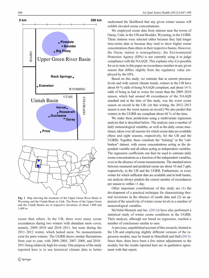
ozone than others. In the UB, there were many ozoneexceedances during two winters with abundant snow cover,namely, 2009–2010 and 2010–2011, but none during the2011–2012 winter, which lacked snow. No measurementsexist for prior winters. The UGRB shows similar fluctuationsfrom year to year, with 2004–2005, 2007–2008, and 2010–2011 being relatively high for ozone. One purpose of the studyreported here is to use historical climate data to better

understand the likelihood that any given winter season willexhibit elevated ozone concentrations.

We employed ozone data from stations near the towns ofOuray, Utah, in the UB and Boulder, Wyoming, in the UGRB.These stations were selected either because they had longertime-series data or because they tend to show higher ozoneconcentrations than others in their respective basins. However,the Ouray station is nonregulatory; the EnvironmentalProtection Agency (EPA) is not currently using it to judgecompliance with the NAAQS. This explains why it is possiblefor us to state in this paper an exceedance number in any givenseason that differs slightly from the regulatory value em-ployed by the EPA.

Based on this study, we estimate that at current precursorlevels and with current climate trends, winters in the UB haveabout 44 % odds of being NAAQS compliant, and about 14 %odds of being as bad or worse for ozone than the 2009–2010season, which had around 40 exceedances of the NAAQSstandard and at the time of this study, was the worst ozoneseason on record in the UB. (At this writing, the 2012–2013season is now the worst season on record.) We also predict thatwinters in the UGRB are compliant about 60 % of the time.

We make these predictions using a multivariate regressionanalysis that is described below. The analysis uses a number ofdaily meteorological variables, as well as the daily ozone max-imum, taken over all seasons for which ozone data are available(three and eight seasons, respectively, for the UB and theUGRB). Together, these constitute the “training” or the “cali-bration” dataset, with ozone concentrations acting as the de-pendent variable and all others acting as independent variables.The regression coefficients can then be used to estimate dailyozone concentrations as a function of the independent variables,even in the absence of ozonemeasurements. The standard errorsbetween measured and predicted ozone are about 10 and 5 ppb,respectively, in the UB and the UGRB. Furthermore, in everywinter for which sufficient data are available and in both basins,our analysis always predicts the correct number of exceedancesper season to within ±1 day.

Other important contributions of this study are (1) thedevelopment of a practical technique for characterizing ther-mal inversions in the absence of sonde data and (2) an ap-praisal of the sensitivity of winter ozone levels to a number ofmeteorological variables.

McVehil-Monnett and Inc. (2011)) have also performed astatistical study of winter ozone conditions in the UGRB.Their analysis, although not based on regression, reached anumber of conclusions similar to ours.

A previous, unpublished account of this research, limited tothe UB and employing slightly different versions of the re-gression models, may be found in Mansfield and Hall (2013).Since then, there have been a few minor adjustments to themodels, but the results reported here are in qualitative agree-ment with that report.

Fig. 1 Map showing the locations of the Upper Green River Basin inWyoming and the Uintah Basin in Utah. The floors of the Upper Greenand the Uintah Basins are at respective elevations of about 1,900 and1,400 m

688 Air Qual Atmos Health (2013) 6:687–699

Model description: quadratic regression

Since standards of ozone compliance are based on daily ozonevalues, usually the daily maximum in the 8-h running average,we have found it convenient to employ daily values of all thevariables, usually using a daily maximum or a daily average.See below for the complete specifications of the daily vari-ables employed. The value of an independent variable will bedenoted x jα, which represents the value of variable j on dayα . (Our subscripting convention in this paper is that Romanindices specify the type of variable while Greek indices spec-ify the day.) The dependent variable will be denoted yα, whichwill always represent the daily maximum in the 8-h runningaverage ozone concentration at some monitoring site on dayα .

The regression model consists of the following formula:

yα ¼ AþXj

B jxjα þXj≤ k

Cjkxjαxkα ð1Þ

where yα designates the ozone concentration on day α aspredicted by the model. The coefficients A , Bj, and Cjk areadjusted to minimize the following function:

S ¼Xα

Wα yα−yα� �2

ð2Þ

The Wα terms are weight factors that increase the flexibil-ity of the model and whose assignment is explained below.The overall quality of fit can be gauged either with thestandard deviation

σ ¼ 1

N

Xα

yα−yα� �2" #1=2

ð3Þ

whereN is the total number of days in the calibration set or thestandard error

ε ¼ 1

N

Xα

yα−yα��� ��� ð4Þ

Minimization of S with respect to A , Bj, andCjk is achievedthrough a straightforward Gauss–Jordan elimination.

Equation (1) is an example of a quadratic regression. Linearregressions, for which the quadratic terms in Eq. (1) are notincluded are, of course, very popular. We decided to includequadratic terms to enhance the flexibility of the model. Forexample, the quadratic terms allow for synergistic interactionsamong the variables.

The model is operated in either a “calibration” mode or a“prediction” mode. The “calibration set” is a set of days for

which all independent variables, Xjα, and all dependent vari-ables, yα or the ozone concentrations, are known, and cali-bration consists of determining the coefficients A , Bj, and Cjk

that optimize Eq. (2) over all days in the set. The “predictionset” is a set of days for which all Xjα are known. Theprediction mode consists of using the coefficients obtainedduring calibration to predict ozone concentrations for everyday in the prediction set. Because ozone measurements are notused in prediction, the prediction set is generally larger thanthe calibration set.

In particular, we include in the prediction set days thatpredate the beginning of winter ozone measurements in thesebasins, going back to 1950 in the UB and 1997 in the UGRB.(We started this study with historical data to the 1990s in bothbasins, but then decided to extend the UB study for an addi-tional 40 years, in order better to test for long-range datatrends.) In so doing, we are not implying that past ozoneprecursor concentrations are comparable to their contempo-rary levels. Rather, the objective is to use historical climatedata to determine the likelihood that a given winter season,under typical present-day precursor concentrations, woulddevelop high ozone levels.

Meteorological variables

In this section, we describe the meteorological variables usedin the model, including definitions and sources. As mentionedabove, the model is based on daily values of the variables, sohere we also explain how a daily value for each variable hasbeen defined. “Acronyms for variables” describes our abbre-viation system for variable names. “Eight-hour ozone concen-trations,” “Basin lapse rate, basin temperature, and consecu-tive days under inversion,” “Average basin snow depth,”“Midday solar angle,” and “Daily average wind speed, rela-tive humidity, and barometric pressure” describe in detail howeach variable was assigned. Table 1 lists statistical propertiesof the variables used.

Acronyms for variables

For convenience, we employ acronyms to designate all mete-orological variables. The complete acronym consists of twoparts. The first part codes for the type of variable, while thesecond codes for the applicable basin. For example, LR:UBwill be used to designate the lapse rate defined for the UintahBasin.

Eight-hour ozone concentrations

Running eight-hour average ozone concentrations (O8) atsites near the towns of Ouray, Utah, in the UB and Boulder,Wyoming, in the UGRB, were obtained from a website

Air Qual Atmos Health (2013) 6:687–699 689

maintained by the EPA (2012). The Ouray dataset includesthree winter seasons: 2009–2010, 2010–2011, and 2011–2012. No prior measurements exist. The Boulder datasetcovers eight winter seasons, beginning with 2004–2005 andending with 2011–2012. In most cases, the datasets wereselected to include the winter period from mid-December tomid-March. Units employed for O8 are parts per billion byvolume.

Basin lapse rate, basin temperature, and consecutive daysunder inversion

A temperature inversion is indicated when the temperature ofthe atmosphere increases with altitude, and experience indi-cates that inversions are required for winter ozone formation.Inversions are characterized by the so-called lapse rate (LR)(Seinfeld and Pandis 2006):

Λ ¼ −dT

dzð5Þ

where T represents temperature and z the altitude. By thisdefinition, a negative lapse rate indicates a temperature inver-sion. Lapse rates are determined by sonde measurements,which are obviously not available day in and day out. There-fore, we developed the following approach to estimate a dailylapse rate for a given basin. Daily temperature data at a set of

meteorological stations from throughout each basin at variousaltitudes and at all available dates between about 1950 and2012 (UB) or about 1990 and 2012 (UGRB) were assembledfrom the database maintained by the Utah Climate Center(2012) (See Online Resource 1 for lists and maps of stationscontributing data for this study, and for the selection criteriaused to select stations.) For any given date, we construct aleast-squares linear correlation between maximum daily tem-perature and altitude, employing data from all stationsreporting a maximum temperature for the day. The LR forany given day is defined operationally as the negative of theslope of the correlation line. Figure 2 shows the linear corre-lations for four selected days in the UB. The slope is negativeon typical summer days, but positive for winter days withinversions. We express LR in Kelvin/kilometer.

The linear-least-squares fit to the temperature–altitude dataalso permits us to define a daily, basin-wide temperature (BT).We take BT to be the value at which the least-squares lineintersects an altitude near the floor (1,400 and 1,900 m, re-spectively) of the basin. Our units for BT are degrees Celsius.

Because ozone precursor concentrations are expected toaccumulate over persistent, multiday inversions, we have intro-duced the variable consecutive days under an inversion (CDI).The value of CDI(α) is 0 on any day α for which LR(α) (thelapse rate) is positive. If LR(α) (i.e., one day’s lapse rate) isnegative while LR(α −1) (i.e., the previous day’s lapse rate) ispositive, then CDI(α)=1 day. If LR(α) and LR(α−1) are bothnegative, then CDI(α)=CDI (α−1)+1 day.

Average basin snow depth

Snow depth (SD) data were also obtained from the UtahClimate Center (2012) using the same stations as for the LRcalculation. However, we have found occasional problemswith the quality of the data. (For example, one station mayreport a snow depth of 0 when all others report abundantsnow.) Therefore, the following procedure was employed:For any given day, we calculated an average snow depth byaveraging over all stations reporting a depth, interpreting “T”(trace) as 10 mm. We then rejected any measurement that fellmore than 2 standard deviations away from the mean for theday. After that rejection, a new mean was calculated. Unitsemployed here for SD are millimeters.

Midday solar angle

The solar angle (SA) at its midday extremum was calculatedusing formulas found in Finlayson-Pitts and Pitts (2000)),using coordinates of the towns of Roosevelt, Utah (40.30°,−109.99°) and Boulder, Wyoming (42.719°, −109.753°), forthe UB and the UGRB, respectively. We employ units ofdegrees and observe the convention that 0 and 90° solar anglesrefer to the zenith and the horizon, respectively.

Table 1 The ranges, means, and standard deviations of the variousvariables in the calibration sets of the various models

Minimum Maximum Mean SD

Uintah Basin datasets

O8:UB (ppb) 21 139 64 26

LR:UB (K/km) −21 14 0 8

SD:UB (mm) 0 370 149 105

SA:UB (°) 42 64 57 6

BT:UB (°C) −18 14 −1 7

CDI:UB (days) 0 43 5 10

WS:UB (m/s) 0.2 7.4 1.2 1.0

RH:UB (%) 29 97 74 12

BP:UB (bar) 0.816 0.854 0.839 0.007

Upper Green River Basin datasets

O8:UGRB (ppm) 22 123 50 13

LR:UGRB (m/s) −68 30 −1 13

SD:UGRB (mm) 46 752 361 150

SA:UGRB (°) 45 66 58 7

BT:UGRB (°C) −29 14 −2 6

CDI:UGRB (days) 0 8 0.9 1.4

WS:UGRB (m/s) 0 8.6 2.8 1.6

RH:UGRB (%) 37 94 75 9

BP:UGRB (bar) 0.763 0.801 0.785 0.006

690 Air Qual Atmos Health (2013) 6:687–699

Daily average wind speed, relative humidity, and barometricpressure

Pre- and post-2005 data for these three variables were ob-tained from websites maintained by the National Oceanic andAtmospheric Association (NOAA), the Unedited LocalClimatological Data (ULCD), and Quality Controlled LocalClimatological Data (QCLCD) databases, respectively(NOAA:NCDC 2012). We used the datasets from the VernalMunicipal and the Big Piney-Marbleton Regional Airports,respectively, to represent the UB and the UGRB. The ULCDand QCLCD databases include hourly observations of allthree variables, which we averaged to obtain a daily variable.Units employed for wind speed (WS), relative humidity (RH),and barometric pressure (BP) are meters per second, percent,and bars, respectively.

Climatic observations based on the data

Figure 3 shows the average lapse rate on any particular calen-dar day for both basins. It indicates that thermal inversions arevery common in both basins in the winter. It also indicates thatwinter lapse rates display a higher variability than those ofsummer.

Figure 4 displays the probability that any given calendarday in the respective basins has snow cover (red, defined

operationally as a day with SD>50 mm), has an inversion(blue, defined operationally as a day with LR<0), or simulta-neously has an inversion and snow cover (green). Both actualdata and best-fit Gaussian distributions (truncated at 1 for thecase of snow cover in UGRB) are displayed. By definition, thegreen traces in Fig. 4 must lie below the blue and red traces(although this requirement does not extend to the Gaussianfits). The fact that all three lie close together for the UBindicates that snow cover plays an important role in stabilizinginversions there. In the UGRB, on the other hand, we seeinversions occurring in the absence of snow cover, in spring orfall, for example. Figures 3 and 4 indicate that January is thepeak month in both basins for snow cover and inversions.

Model development and performance, calibration mode

Because daily data are not always available, we are forced tocompromise between having a diverse set of independentvariables and having a large number of days in the predictionset. To explore optimal trade-offs, we have constructed a fewdifferent models of the ozone system of each basin. Thesemodels are summarized in Tables 2 and 3. Two of the models,Ouray-8 and Ouray-5, are applicable to the UB, and use ozoneconcentration measurements from a station near Ouray, Utah.The other three models, Boulder-5, Boulder-6, and Boulder-8,are applicable to the UGRB and refer to an ozone station near

Fig. 2 Temperature–altitudecorrelations for four typical daysin the Uintah Basin. Each point inthe figure is labelled with anumber that corresponds to a mapand table in the supplementaryinformation. The numerical valueof the daily lapse rate in K/km andthe r2 correlation coefficients arealso displayed

Air Qual Atmos Health (2013) 6:687–699 691

Boulder, Wyoming. In each case, the numerical suffix indi-cates the number of independent variables used by the model.Specifically, Ouray-8 and Boulder-8 use the following eightindependent variables: (1) LR, (2) SD, (3) BT, (4) SA, (5)CDI, (6) WS, (7) RH, and (8) BP. Boulder-6 is obtained bydropping RH and BP, and Boulder-5 by also dropping WS.Ouray-5 is obtained from Ouray-8 by dropping RH, BP, andWS. By eliminating certain variables, we are able to expandthe prediction set, since, for example, available wind speeddata does not extend as far back as available snow depth data.The question, however, is the degree to which the predictivepower of the model deteriorates with the omission of certainvariables. As explained below, we have determined thatOuray-5 and Boulder-6 are the models of choice for optimiz-ing the trade-off mentioned above.

The weight factors shown in Eq. (2) permit us to apportiongreater weights to some days in the calibration set than to

others. We used the following formula to assign a weight toeach day in each calibration set:

Wα ¼ yαbc !p

ð6Þ

As explained above, yα is the ozone concentration for dayα .bc is the unit concentration of 1 ppb—its presence in Eq. (6)is a formality that renders Wα dimensionless—and p is anadjustable exponent. Selecting p >0 imparts greater weights tohigh-ozone days and vice versa. The value of p was adjusted(by trial and error) to optimize the agreement between theactual and the predicted number of days per season that theNAAQS ozone standard of 75 ppb is exceeded. The p valuesemployed in each model are given in Table 2.

The regression coefficients for each model are given inOnline Resource 2.

a

b

Fig. 3 Average daily lapse rate in the Uintah Basin (a) and the UpperGreen River Basin (b). The red traces are the lapse rate itself; the greentraces are displaced above and below by one standard deviation. Theblack curves are a filtered representation of the red trace

a

b

Fig. 4 The probability that a given day in the Uintah Basin (a) and theUpper Green River Basin (b) has mean snow depth >50 mm (red), hasnegative lapse rate (blue), or simultaneously has both (green). Evaluatedover about 60 years for the Uintah Basin and about 20 for the UpperGreen River Basin. Also shown are best-fit Gaussian distributions

692 Air Qual Atmos Health (2013) 6:687–699

Figure 5 plots the predicted against the measured ozone con-centration for each day in the calibration set of Ouray-5. (Similarplots for all five models are given in Online Resource 3.) Ifthe model were able to make exact predictions, then all pointswould of course lie on the diagonal. The standard deviationsand errors for eachmodel are given in Table 2. In any case, theagreement between actual and predicted ozone concentrationsis good enough that we can make useful predictions.Agreement is especially good at lower ozone concentrations,but for reasons we do not understand, the models consistentlyunderestimate the highest ozone concentrations. We havebeen able to compensate somewhat for the poorer perfor-mance at higher concentrations through the introduction ofthe weight factors defined in Eq. (6), so that the models predictvery accurately the number of exceedance days per season.

Figure 6 show the response of Ouray-8 and Boulder-8 tovariations in the independent variables. The ozone concentra-tion as predicted by the model is plotted along the ordinate,while along the abscissa is displayed the displacement of eachvariable from its mean value. All curves converge at a pointnear the center of each graph that represents the model pre-diction (75.2 and 51.0 ppb, respectively) when all independentvariables are held at their mean values (μ). Then, each indi-vidual curve shows how the predicted concentration varies asone of the variables is allowed to change from a low valueequal to two standard deviations below its mean (μ −2σ ) totwo standard deviations above (μ +2σ ), while holding allother variables at their means. The means (μ) and standarddeviations (σ ) of each variable are tabulated in Table 1. By

virtue of their definitions, CDI, WS, and SD can never benegative. Whenever μ −2σ is negative for these variables, theassociated curve terminates at the zero of the variable, ratherthan at μ −2σ . Because this is a quadratic regression, each ofthe curves in Fig. 6 is a parabola. (A linear regression wouldhave produced straight lines.) Obviously, the variables withhigh sensitivity show large vertical displacements on thesegraphs. Table 4 shows each variable ranked according to itsmaximum vertical displacement in Fig. 6.

We can make all of the following observations about thecurves in Fig. 6 and the sensitivities tabulated in Table 4. Itshould be remembered that these curves show the behavior ofthe models, not of the actual ozone systems of the two basins.Nevertheless, they suggest clues to the operation of the actualsystems:

1. The magnitudes of the sensitivities are greater for the UB.Of the two basins, it generally forms more ozone.

2. SA is the single strongest predictor of ozone concentrationin both basins. The sign of the SA correlation is appropriate,since we are measuring solar angle relative to the zenith.

3. The sensitivity of LR relative to that of other variables issmaller than we might have anticipated, since we haveassumed that LR would reflect both the depth and thestability of the mixing layer. On the other hand, the dataseem to indicate that in late winter, significant ozoneevents can occur even when the lapse rate is trendingpositive (Mansfield and Hall 2013). The relative sensitiv-ities of SA and LR support this observation.

Table 2 Variable sets and other characteristics of each of the models

Ouray-8 Ouray-5 Boulder-8 Boulder-6 Boulder-5

Dependent variable O8:UB O8:UB O8:UGRB O8:UGRB O8:UGRB

Independent variables LR:UB SD:UBSA:UB BT:UBCDI:UB WS:UBRH:UB BP:UB

LR:UB SD:UBSA:UB BT:UBCDI:UB

LR:UGRB SD:UGRBSA:UGRB BT:UGRBCDI:UGRB WS:UGRBRH:UGRB BP:UGRB

LR:UGRB SD:UGRBSA:UGRB BT:UGRBCDI:UGRB WS:UGRB

LR:UGRB SD:UGRBSA:UGRB BT:UGRBCDI:UGRB

σ (ppb) 11.9 13.6 7.6 7.7 9.9

ε (ppb) 8.6 10.1 5.4 5.5 7.2

p value −1 −1 0.5 0.5 1.75

Table 3 Calibration and predic-tion sets of the models Calibration set Prediction set

Ouray-5 239 days: mid-Dec 2009 to mid-Mar 2010; mid-Dec2010 to mid-Mar 2011; Jan and Feb 2012

Jan 1950 to Feb 2012, but with gaps in1950s

Ouray-8 Same as Ouray-5 Jan 2005 to Feb 2012, but with gaps

Boulder-5 594 days: early Feb 2005 to mid-Mar 2005; mid-Decto mid-Mar for each season from 2005–2006 to2010–2011; mid-Dec 2011 to early Feb 2012

Dec 1990 to Jan 2012, but with gaps.

Boulder-6 Same as Boulder-5 Mar 1998 to Jan 2012

Boulder-8 Same as Boulder-5 Same as Boulder-6

Air Qual Atmos Health (2013) 6:687–699 693

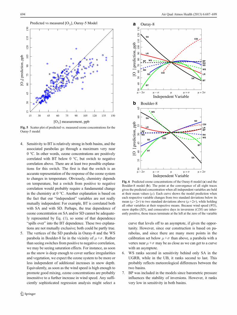
4. Sensitivity to BT is relatively strong in both basins, and theassociated parabolas go through a maximum very near0 °C. In other words, ozone concentrations are positivelycorrelated with BT below 0 °C, but switch to negativecorrelation above. There are at least two possible explana-tions for this switch. The first is that the switch is anaccurate representation of the response of the ozone systemto changes in temperature. Obviously, chemistry dependson temperature, but a switch from positive to negativecorrelation would probably require a fundamental changein the chemistry at 0 °C. Another explanation is based onthe fact that our “independent” variables are not reallymutually independent: For example, BT is correlated bothwith SA and with SD. Perhaps, the true dependence ofozone concentration on SA and/or SD cannot be adequate-ly represented by Eq. (1), so some of that dependence“spills over” into the BT dependence. These two explana-tions are not mutually exclusive; both could be partly true.

5. The vertices of the SD parabola in Ouray-8 and the WSparabola in Boulder-8 lie in the vicinity of μ +σ . Ratherthan seeing switches from positive to negative correlation,we may be seeing saturation effects. For instance, as soonas the snow is deep enough to cover surface irregularitiesand vegetation, we expect the ozone system to be more orless independent of additional increases in snow depth.Equivalently, as soon as the wind speed is high enough topromote good mixing, ozone concentrations are probablyinsensitive to a further increase in wind speed. Any suffi-ciently sophisticated regression analysis might select a

curve that levels off to an asymptote, if given the oppor-tunity. However, since our construction is based on pa-rabolas, and since there are many more points in thecalibration set below μ +σ than above, a parabola with avertex near μ +σ may be as close as we can get to a curvewith an asymptote.

6. WS ranks second in sensitivity behind only SA in theUGRB, while in the UB, it ranks second to last. Thisprobably reflects meteorological differences between thetwo basins.

7. BP was included in the models since barometric pressureinfluences the stability of inversions. However, it ranksvery low in sensitivity in both basins.

Fig. 5 Scatter plot of predicted vs. measured ozone concentrations for theOuray-5 model

a

b

Fig. 6 Predicted ozone concentrations of the Ouray-8 model (a) and theBoulder-8 model (b). The point at the convergence of all eight tracesgives the predicted concentration when all independent variables are heldat their mean values (μ). Each curve shows the model prediction wheneach respective variable changes from two standard deviations below itsmean (μ−2σ) to two standard deviations above (μ +2σ), while holdingall other variables at their respective means. Because wind speed (WS),snow depths (SD), and consecutive days in inversions (CDI) are inher-ently positive, those traces terminate at the left at the zero of the variable

694 Air Qual Atmos Health (2013) 6:687–699

8. Ouray-8 has an especially high sensitivity to CDI. Nodoubt this reflects the effects of precursor buildup duringmultiday inversions.

As mentioned above, Ouray-5 and Boulder-6 are the modelsof choice. There are three arguments in favor of these selections:

1. Because of weak sensitivities to some variables, as re-vealed in Fig. 6 and in Table 4, Ouray-8 can tolerate theomission of RH, WS, and BP, while Boulder-8 can toler-ate the omission of RH and BP, but not of WS.

2. The predictions of Ouray-5 and Boulder-6 for the numberof exceedance days per season are in good agreementwith the actual data.

3. The capacity of Ouray-5 and Boulder-6 to predictexceedances per season is not significantly worse thanthat of Ouray-8 and Boulder-8, respectively.

Data supporting the second and third arguments arepresented in Online Resource 4.

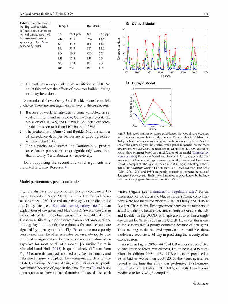
Model performance, prediction mode

Figure 7 displays the predicted number of exceedances be-tween December 15 and March 15 in the UB for each of 63seasons since 1950. The red trace displays our prediction forthe Ouray site (see “Estimates for regulatory sites” for anexplanation of the green and blue traces). Several seasons inthe decade of the 1950s have gaps in the available SD data.These were filled by proportionate assignment among all themissing days in a month, the estimates for such seasons aresignaled by open symbols in Fig. 7a, and are more poorlyconstrained than the other estimates because, obviously, pro-portionate assignment can be a very bad approximation whengaps last for most or all of a month. [A similar figure inMansfield and Hall (2013) is quantitatively different fromFig. 7 because that analysis counted only days in January andFebruary.] Figure 8 displays the corresponding data for theUGRB, covering 15 years. Again, some estimates are poorlyconstrained because of gaps in the data. Figures 7b and 8 useopen squares to show the actual number of exceedances each

winter. (Again, see “Estimates for regulatory sites” for anexplanation of the green and blue symbols.) Ozone concentra-tions were not measured prior to 2010 at Ouray and 2005 atBoulder. There is excellent agreement between the numbers ofactual and the predicted exceedances, both at Ouray in the UBand Boulder in the UGRB, with agreement to within a singleday except for Winter 2008 in the UGRB. However, this is oneof the seasons that is poorly estimated because of data gaps.Thus, as long as the required input data are available, thesemodels are accurate to ±1 day in predicting the severity of anozone season.

As seen in Fig. 7, 28/63=44 % of UB winters are predictedto have three or fewer exceedances, i.e., to be NAAQS com-pliant. In addition, 9/63=14 % of UB winters are predicted tobe as bad or worse than 2009–2010, the worst season onrecord at the time this study was performed. Furthermore,Fig. 8 indicates that about 9/15=60 % of UGRB winters arepredicted to be NAAQS compliant.

Table 4 Sensitivities ofthe displayed models,defined as the maximumvertical displacement ofthe associated curvesappearing in Fig. 6, indescending order

Ouray-8 Boulder-8

SA 76.4 ppb SA 29.3 ppb

CDI 53.9 WS 16.3

BT 45.5 BT 14.2

LR 31.7 SD 14.0

SD 19.6 CDI 7.2

RH 12.4 LR 3.3

WS 12.3 BP 2.3

BP 2.2 RH 1.2

a

b

Fig. 7 Estimated number of ozone exceedances that would have occurredin the indicated season between the dates of 15 December to 15 March, ifthat year had precursor emissions comparable to modern values. Panel ashows the entire 63-year time-series, while panel b focuses on the mostrecent years.Red traces are the results of the Ouray-5model.Blue and greentraces show estimates based on a modification of the model (Estimates forregulatory sites) for sites at Vernal and Roosevelt, Utah, respectively. Thelower dashed line is at 4 days; seasons below this line would have beenNAAQS compliant. The upper dashed line is at 41 days; indicating seasonsthat would have been worse for ozone than 2010.Open symbols (at seasons1950, 1955, 1956, and 1957) are poorly constrained estimates because ofdata gaps.Open squares display actual numbers of exceedances for the threesites: red Ouray, green Roosevelt, and blue Vernal

Air Qual Atmos Health (2013) 6:687–699 695

A very striking feature of the data in Fig. 7 is their broadvariability. Many years are predicted to produce noexceedances, but years with 40 or more exceedances are alsocommon. The data indicate that a typical winter pattern in theUB is the occurrence of a major snowstorm, often inDecember, which creates a snowpack that persists throughabout the end of February. The snowpack acts to stabilizeinversions, setting the stage for many exceedances duringthe rest of the winter. On the other hand, although less typical,some winters see little or no snow, and then ozone remainsclose to background levels, producing no exceedances.

Figure 9 plots mean ozone concentration on any givencalendar day, as predicted by either Ouray-5 or Boulder-6and averaged over all days in the respective prediction sets.Ozone concentrations are predicted to peak in February andMarch in the UB and the UGRB, respectively. As indicated byFig. 4, the likelihood of thermal inversions combined withsnow cover peaks in both basins in January, but peak ozoneseason falls a month or two later because of the effect of solarangle.

Figure 9 also displays daily averages over the calibrationsets, i.e., over days with actual ozone measurements. The twotraces for the UGRB are in good agreement, primarily becausethe prediction set is only about twice as large as the calibrationset and because the calibration set includes enough seasons,eight, that its averages are reasonably representative. Becausethe calibration set for the UB includes only three seasons, theagreement there is understandably poorer. In fact, with onlythree seasons, individual ozone events stand out as majorpeaks in the time series.

Estimates for regulatory sites

As mentioned above, the Ouray site was chosen for this studybecause it provides the longest data sequence, covering threefull winters. However, other ozone monitoring sites near thetowns of Roosevelt and Vernal, Utah, will probably be usedfor regulatory purposes, meaning that it would be informativeto make predictions for these sites as well. Figure 10 displayscorrelations between the 8-h daily maximum for the threesites, for one winter ozone season between 30 December2010 and 11 March 2011. Obviously, the ozone concentrationat Ouray is a good predictor of the concentrations at eitherVernal or Roosevelt. If we let yO, yR, and yV represent,respectively, the daily 8-h maximum in ppb at Ouray,Roosevelt, and Vernal, then the correlation lines are

yR ¼ 7:6ppbþ 0:77yO; R2 ¼ 0:90 ð7Þ

yV ¼ 18:0ppbþ 0:53yO; R2 ¼ 0:80 ð8Þ

We can use Eqs. (7) and (8) to estimate ozone concentra-tions at either Vernal or Roosevelt, given the model predic-tions for Ouray. The results of these estimates for exceedancedays per season appear in Fig. 7. This analysis indicates thatozone concentrations are expected to be lower in Rooseveltthan in Ouray and lower still in Vernal. However, Fig. 7bindicates that this approach underestimates the actual numberof exceedance days in 2011.

Fig. 8 Estimated number of ozone exceedances that would have oc-curred in the UGRB during the indicated season between the dates of 15December to 15 March, if that season had precursor emissions compara-ble to modern values, as predicted by the Boulder-6 model. The dashedline is at 4 days, indicating NAAQS compliance. Open symbols (atseasons 1998, 2007, and 2008) are poorly constrained estimates becauseof data gaps. Open squares indicate actual numbers of exceedances

Fig. 9 Mean estimated ozone levels by day for the Ouray-5 model (blue,light) and the Boulder-6 model (red , light). Also shown are the meanstaken over actual measurements at Ouray (blue, heavy) and at Boulder(red , heavy ). Because of excessive noise, these latter are actuallydisplayed as 7-day running averages

696 Air Qual Atmos Health (2013) 6:687–699

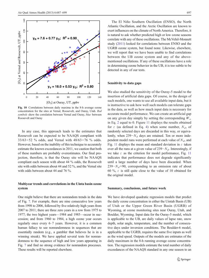
In any case, this approach leads to the estimates thatRoosevelt can be expected to be NAAQS compliant with33/63=52 % odds, and Vernal with 48/63=76 % odds.However, based on the inability of this technique to accuratelyestimate the known exceedances in 2011, we caution that bothof these numbers are probably overestimates. Our final pro-jection, therefore, is that the Ouray site will be NAAQScompliant each season with about 44 % odds, the Rooseveltsite with odds between about 44 and 52 %, and the Vernal sitewith odds between about 44 and 76 %.

Multiyear trends and correlations in the Uinta basin ozonesystem

One might believe that there are nonrandom trends in the dataof Fig. 7. For example, there are nine consecutive low yearsfrom 1998 to 2006, followed by five relatively high years from2007 to 2011; there are three zero years in a row from 1975 to1977; the two highest years—1984 and 1985—occur in suc-cession; and from 1960 to 1984, a high ozone year occursregularly once every 6–7 years. However, it is a commonhuman fallacy to see nonrandomness in sequences that areessentially random (e.g., a gambler that believes he is in awinning streak). We have applied several tests for nonran-domness to the sequence of high and low years appearing inFig. 7 and find no strong evidence for nonrandom processes.These results will be reported elsewhere.

The El Niño Southern Oscillation (ENSO), the NorthAtlantic Oscillation, and the Arctic Oscillation are known toexert influences on the climate of North America. Therefore, itis natural to ask whether predicted high or low ozone seasonscorrelate with any of these oscillations. The McVehil-Monnettstudy (2011) looked for correlations between ENSO and theUGRB ozone system, but found none. Likewise, elsewhere,we will report that we have been unable to find correlationsbetween the UB ozone system and any of the above-mentioned oscillations. If any of these oscillations have a rolein determining ozone behavior in the UB, it is too subtle to bedetected in any of our tests.

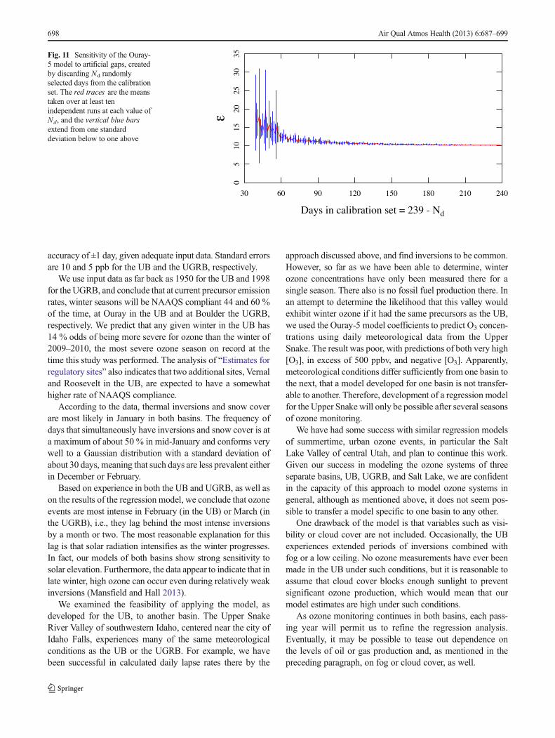
Sensitivity to data gaps

We also studied the sensitivity of the Ouray-5 model to theinsertion of artificial data gaps. Of course, in the design ofsuch models, one wants to use all available input data, but itis instructive to ask how well such models can tolerate gapsin the data, as well as how much input data is necessary foraccurate model performance. We can create an artificial gapon any given day simply by setting the corresponding Wα

in Eq. 2 equal to 0. Figure 11 displays the results obtainedfor ε (as defined in Eq. 4) when some number, Nd, ofrandomly selected days are discarded in this way, or equiva-lently, when 239−Nd days are retained. Ten or more inde-pendent model runs were performed at each value of Nd, andFig. 11 displays the mean and standard deviation in ε takenover all the runs at a given value of 239−Nd. Interestingly, ifwe take ε as the criterion for model performance, Fig. 11indicates that performance does not degrade significantlyuntil a large number of days have been discarded. When239−Nd≈90, corresponding to an omission rate of about60 %, ε is still quite close to the value of 10 obtained forthe original model.

Summary, conclusions, and future work

We have developed quadratic regression models that predictthe daily ozone concentration in either the Uintah Basin (UB)of Utah or the Upper Green River Basin (UGRB) ofWyoming, at ozone monitoring sites near Ouray, Utah, andBoulder, Wyoming. Input data for the Ouray-5 model, whichis applicable to the UB, are daily values of lapse rate, snowdepth, solar angle, temperature, and the number of consecu-tive days under inversion conditions. The Boulder-6 model,applicable to the UGRB, requires the same five inputs as wellas the wind speed. Outputs of the models are estimates of thedaily maximum in the 8-h running average ozone concentra-tion. The regression models estimate the total number of dailyexceedances of the NAAQS standard in any one season to an

Fig. 10 Correlations between daily maxima in the 8-h average ozoneconcentration for the sites at Vernal, Roosevelt, and Ouray, Utah. Redsymbols show the correlation between Vernal and Ouray, blue betweenRoosevelt and Ouray

Air Qual Atmos Health (2013) 6:687–699 697

accuracy of ±1 day, given adequate input data. Standard errorsare 10 and 5 ppb for the UB and the UGRB, respectively.

We use input data as far back as 1950 for the UB and 1998for the UGRB, and conclude that at current precursor emissionrates, winter seasons will be NAAQS compliant 44 and 60 %of the time, at Ouray in the UB and at Boulder the UGRB,respectively. We predict that any given winter in the UB has14 % odds of being more severe for ozone than the winter of2009–2010, the most severe ozone season on record at thetime this study was performed. The analysis of “Estimates forregulatory sites” also indicates that two additional sites, Vernaland Roosevelt in the UB, are expected to have a somewhathigher rate of NAAQS compliance.

According to the data, thermal inversions and snow coverare most likely in January in both basins. The frequency ofdays that simultaneously have inversions and snow cover is ata maximum of about 50 % in mid-January and conforms verywell to a Gaussian distribution with a standard deviation ofabout 30 days, meaning that such days are less prevalent eitherin December or February.

Based on experience in both the UB and UGRB, as well ason the results of the regression model, we conclude that ozoneevents are most intense in February (in the UB) or March (inthe UGRB), i.e., they lag behind the most intense inversionsby a month or two. The most reasonable explanation for thislag is that solar radiation intensifies as the winter progresses.In fact, our models of both basins show strong sensitivity tosolar elevation. Furthermore, the data appear to indicate that inlate winter, high ozone can occur even during relatively weakinversions (Mansfield and Hall 2013).

We examined the feasibility of applying the model, asdeveloped for the UB, to another basin. The Upper SnakeRiver Valley of southwestern Idaho, centered near the city ofIdaho Falls, experiences many of the same meteorologicalconditions as the UB or the UGRB. For example, we havebeen successful in calculated daily lapse rates there by the

approach discussed above, and find inversions to be common.However, so far as we have been able to determine, winterozone concentrations have only been measured there for asingle season. There also is no fossil fuel production there. Inan attempt to determine the likelihood that this valley wouldexhibit winter ozone if it had the same precursors as the UB,we used the Ouray-5 model coefficients to predict O3 concen-trations using daily meteorological data from the UpperSnake. The result was poor, with predictions of both very high[O3], in excess of 500 ppbv, and negative [O3]. Apparently,meteorological conditions differ sufficiently from one basin tothe next, that a model developed for one basin is not transfer-able to another. Therefore, development of a regression modelfor the Upper Snake will only be possible after several seasonsof ozone monitoring.

We have had some success with similar regression modelsof summertime, urban ozone events, in particular the SaltLake Valley of central Utah, and plan to continue this work.Given our success in modeling the ozone systems of threeseparate basins, UB, UGRB, and Salt Lake, we are confidentin the capacity of this approach to model ozone systems ingeneral, although as mentioned above, it does not seem pos-sible to transfer a model specific to one basin to any other.

One drawback of the model is that variables such as visi-bility or cloud cover are not included. Occasionally, the UBexperiences extended periods of inversions combined withfog or a low ceiling. No ozone measurements have ever beenmade in the UB under such conditions, but it is reasonable toassume that cloud cover blocks enough sunlight to preventsignificant ozone production, which would mean that ourmodel estimates are high under such conditions.

As ozone monitoring continues in both basins, each pass-ing year will permit us to refine the regression analysis.Eventually, it may be possible to tease out dependence onthe levels of oil or gas production and, as mentioned in thepreceding paragraph, on fog or cloud cover, as well.

Fig. 11 Sensitivity of the Ouray-5 model to artificial gaps, createdby discarding Nd randomlyselected days from the calibrationset. The red traces are the meanstaken over at least tenindependent runs at each value ofNd, and the vertical blue barsextend from one standarddeviation below to one above

698 Air Qual Atmos Health (2013) 6:687–699

Acknowledgments This research was funded by the Uintah ImpactMitigation Special Services District, Uintah County, Utah, USA, and bythe Utah Science Technology and Research Initiative.

References

EPA (2012) Air data. United States Environmental Protection Agency.www.epa.gov/airdata/ad_maps.html

Finlayson-Pitts BJ, Pitts JN (2000) Chemistry of the upper and loweratmosphere. Academic, San Diego

Mansfield M, Hall C (2013) The potential for ozone production in theUintah Basin: a climatological analysis. In: Lyman S, Shorthill H (eds)Final report: 2012 Uintah BasinWinter Ozone and Air Quality Study.Utah State University, document no. CRD13-320.32, February 1,2013. rd.usu.edu/files/uploads/ubos_2011-12_final_report.pdf

Martin R,Moore K,MansfieldM,Hill S, Harper K, Shorthill (2011) Finalreport: Uinta BasinWinter Ozone and Air Quality Study: December

2010–March 2011. Energy Dynamics Laboratory, Utah State Uni-versity Research Foundation, document no. EDL/11-039, June 14,2011. rd.usu.edu/files/uploads/edl_2010-11_report_ozone_final.pdf

McVehil-Monnett Associates, Inc. (2011) Ground-level ozone andmeteorological parameter correlation analysis for the upperGreen River Basin. Report to Wyoming Department of Environ-mental Quality, October 2011, MMA project no. 2451-11. www.mcvehil-monnett.com

NOAA:NCDC (2012) National Climatic Data Center, National Oceanicand Atmospheric Administration. www.ncdc.noaa.gov/land-based-station-data/land-based-datasets

Schnell RC, Oltmans SJ, Neeley RR, Endres MS, Molenar JV, White AB(2009) Rapid photochemical production at high concentrations in arural site during winter. Nat Geosci 2:120–122

Seinfeld JH, Pandis SN (2006) Atmospheric chemistry and physics, 2ndedn. Wiley-Interscience, Hoboken

Stoeckenius T, Ma L (2010) Final report: a conceptual model of winterozone episodes in Southwest Wyoming, Environ, Novato

Utah Climate Center (2012) Utah Climate Center, Utah State University.www.climate.usurf.usu.edu

Air Qual Atmos Health (2013) 6:687–699 699