Statistical Analysis of Fragility Curves -...
173
ISSN 1520-295X Statistical Analysis of Fragility Curves by M. Shinozuka, M.Q. Feng, H. Kim, T. Uzawa and T. Ueda Department of Civil and Environmental Engineering University of Southern California Los Angeles, California 90089-2531 Technical Report MCEER-03-0002 June 16, 2003 This research was conducted at the University of Southern California and was supported by the Federal Highway Administration under contract number DTFH61-92-C-00106. .
Transcript of Statistical Analysis of Fragility Curves -...

ISSN 1520-295X
Statistical Analysis of Fragility Curves
by
M. Shinozuka, M.Q. Feng, H. Kim, T. Uzawa and T. UedaDepartment of Civil and Environmental Engineering
University of Southern CaliforniaLos Angeles, California 90089-2531
Technical Report MCEER-03-0002
June 16, 2003
This research was conducted at the University of Southern California and was supportedby the Federal Highway Administration under contract number DTFH61-92-C-00106.
.

NOTICEThis report was prepared by the University of Southern California as a result ofresearch sponsored by the Multidisciplinary Center for Earthquake EngineeringResearch (MCEER) through a contract from the Federal Highway Administration.Neither MCEER, associates of MCEER, its sponsors, the University of SouthernCalifornia, nor any person acting on their behalf:
a. makes any warranty, express or implied, with respect to the use of any infor-mation, apparatus, method, or process disclosed in this report or that such usemay not infringe upon privately owned rights; or
b. assumes any liabilities of whatsoever kind with respect to the use of, or thedamage resulting from the use of, any information, apparatus, method, or pro-cess disclosed in this report.
Any opinions, findings, and conclusions or recommendations expressed in thispublication are those of the author(s) and do not necessarily reflect the views ofMCEER or the Federal Highway Administration.
Statistical Analysis of Fragility Curves
by
M. Shinozuka1, M.Q. Feng2, H. Kim3, T. Uzawa4 and T. Ueda4
Publication Date: June 16, 2003Submittal Date: January 18, 2000
Technical Report MCEER-03-0002
Task Numbers 106-E-7.3.5 and 106-E-7.6
FHWA Contract Number DTFH61-92-C-00106
1 Fred Champion Professor, Department of Civil and Environmental Engineering, University ofSouthern California; now Distinguished Professor and Chair, Department of Civil Engineering,University of California, Irvine
2 Associate Professor, Department of Civil Engineering, University of California, Irvine3 Visiting Scholar, Department of Civil and Environmental Engineering, University of Southern Califor-
nia4 Visiting Researcher, Department of Civil and Environmental Engineering, University of Southern
California
MULTIDISCIPLINARY CENTER FOR EARTHQUAKE ENGINEERING RESEARCHUniversity at Buffalo, State University of New YorkRed Jacket Quadrangle, Buffalo, NY 14261


Preface
The Multidisciplinary Center for Earthquake Engineering Research (MCEER) is a national centerof excellence in advanced technology applications that is dedicated to the reduction of earthquakelosses nationwide. Headquartered at the University at Buffalo, State University of New York, theCenter was originally established by the National Science Foundation in 1986, as the NationalCenter for Earthquake Engineering Research (NCEER).
Comprising a consortium of researchers from numerous disciplines and institutions throughoutthe United States, the Center’s mission is to reduce earthquake losses through research and theapplication of advanced technologies that improve engineering, pre-earthquake planning andpost-earthquake recovery strategies. Toward this end, the Center coordinates a nationwideprogram of multidisciplinary team research, education and outreach activities.
MCEER’s research is conducted under the sponsorship of two major federal agencies, theNational Science Foundation (NSF) and the Federal Highway Administration (FHWA), and theState of New York. Significant support is also derived from the Federal Emergency ManagementAgency (FEMA), other state governments, academic institutions, foreign governments andprivate industry.
The Center’s FHWA-sponsored Highway Project develops retrofit and evaluation methodologiesfor existing bridges and other highway structures (including tunnels, retaining structures, slopes,culverts, and pavements), and improved seismic design criteria and procedures for bridges andother highway structures. Specifically, tasks are being conducted to:• assess the vulnerability of highway systems, structures and components;• develop concepts for retrofitting vulnerable highway structures and components;• develop improved design and analysis methodologies for bridges, tunnels, and retaining
structures, which include consideration of soil-structure interaction mechanisms and theirinfluence on structural response;
• review and recommend improved seismic design and performance criteria for new highwaysystems and structures.
Highway Project research focuses on two distinct areas: the development of improved design criteria andphilosophies for new or future highway construction, and the development of improved analysis andretrofitting methodologies for existing highway systems and structures. The research discussed in thisreport is a result of work conducted under the existing highway structures project, and was performedwithin Tasks 106-E-7.3.5 and 106-E-7.6, “SRA Validation and Fragility Curves” of that project asshown in the flowchart on the following page.
This report presents methods of developing bridge fragility curves on the basis of statisticalanalysis. Two types of curves are developed. Empirical fragility curves use bridge damage datafrom the past earthquakes, particularly from the 1994 Northridge and 1995 Kobe earthquakes,and analytical fragility curves are constructed for typical bridges in the Memphis, Tennessee areausing nonlinear dynamic analysis. The Los Angeles area expressway network is used as an
iii
iv
example to determine the effectiveness of using these fragility curves to estimate seismicperformance. The conceptual and theoretical treatment dealt with in this study may provide atheoretical basis and practical analysis tools for the development of fragility curves and theirapplication in assessing the seismic performance of transportation networks.
Furthermore, this report has unique pedagogical and archival features in that it (1) summarizesa number of journal and conference papers published earlier together with other unpublishedmaterials arising from this study in a consistent manner, (2) includes damage data obtained fromthe 1994 Northridge and 1995 Hanshin-Awaji (Kobe) earthquake shortly after the events, (3)shows how one can simulate a set of simulated damage data by Monte Carlo techniques, (4)provides statistical procedures for hypothesis testing and estimation of confidence interval for theparameters in the fragility model, irrespective of whether data are empirically or analyticallydeveloped, and (5) actual process of these testing and estimation is guided step-by-step using thearchived damage data.
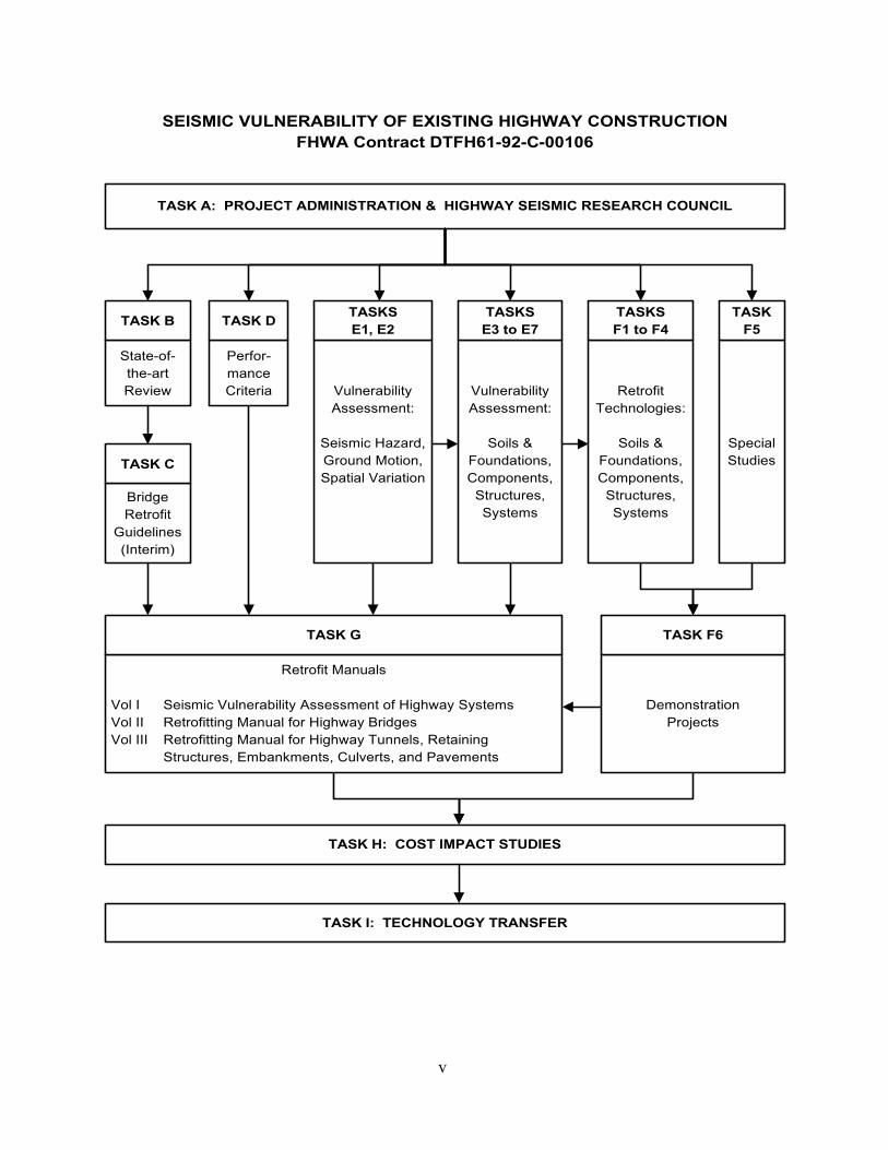
TASK A: PROJECT ADMINISTRATION & HIGHWAY SEISMIC RESEARCH COUNCIL
State-of-the-artReview
TASK B
Perfor-manceCriteria
TASK D
BridgeRetrofit
Guidelines(Interim)
TASK C
VulnerabilityAssessment:
Seismic Hazard,Ground Motion,Spatial Variation
TASKSE1, E2
VulnerabilityAssessment:
Soils &Foundations,Components,
Structures,Systems
TASKSE3 to E7
RetrofitTechnologies:
Soils &Foundations,Components,
Structures,Systems
TASKSF1 to F4
SpecialStudies
TASKF5
TASK H: COST IMPACT STUDIES
TASK I: TECHNOLOGY TRANSFER
SEISMIC VULNERABILITY OF EXISTING HIGHWAY CONSTRUCTIONFHWA Contract DTFH61-92-C-00106
DemonstrationProjects
TASK F6
Retrofit Manuals
Vol I Seismic Vulnerability Assessment of Highway SystemsVol II Retrofitting Manual for Highway BridgesVol III Retrofitting Manual for Highway Tunnels, Retaining
Structures, Embankments, Culverts, and Pavements
TASK G
v


vii
ABSTRACT
This report presents methods of bridge fragility curve development on the basis of statistical
analysis. Both empirical and analytical fragility curves are considered. The empirical fragility
curves are developed utilizing bridge damage data obtained from past earthquakes, particularly
the 1994 Northridge and 1995 Hyogo-ken Nanbu (Kobe) earthquake. Analytical fragility curves
are constructed for typical bridges in the Memphis, Tennessee area utilizing nonlinear dynamic
analysis.
Two-parameter lognormal distribution functions are used to represent the fragility curves. These
two-parameters (referred to as fragility parameters) are estimated by two distinct methods. The
first method is more traditional and uses the maximum likelihood procedure treating each event
of bridge damage as a realization from a Bernoulli experiment. The second method is unique in
that it permits simultaneous estimation of the fragility parameters of the family of fragility
curves, each representing a particular state of damage, associated with a population of bridges.
The method still utilizes the maximum likelihood procedure, however, each event of bridge
damage is treated as a realization from a multi-outcome Bernoulli type experiment.
These two methods of parameter estimation are used for each of the populations of bridges
inspected for damage after the Northridge and Kobe earthquakes and with numerically simulated
damage for the population of typical Memphis area bridges. Corresponding to these two
methods of estimation, this report introduces statistical procedures for testing goodness of fit of
the fragility curves and of estimating the confidence intervals of the fragility parameters. Some
preliminary evaluations are made on the significance of the fragility curves developed as a
function of ground intensity measures other than PGA.
Furthermore, applications of fragility curves in the seismic performance estimation of
expressway network systems are demonstrated. Exploratory research was performed to compare
the empirical and analytical fragility curves developed in the major part of this report with those

viii
constructed utilizing the nonlinear static method currently promoted by the profession in
conjunction with performance-based structural design. The conceptual and theoretical treatment
discussed herein is believed to provide a theoretical basis and practical analytical tools for the
development of fragility curves, and their application in the assessment of seismic performance
of expressway network systems.

ix
ACKNOWLEDGMENT
This study was supported by the Federal Highway Administration under contract DTFH61-92-C-
00106 (Tasks 106-E-7.3.5 and 106-E-7.6) through the Multidisciplinary Center for Earthquake
Engineering Research (MCEER) in Buffalo, NY. The authors wish to express their sincere
gratitude to Dr. Ian Buckle for his support and encouragement and Mr. Ian Friedland for ably
managing the project at MCEER.

xi
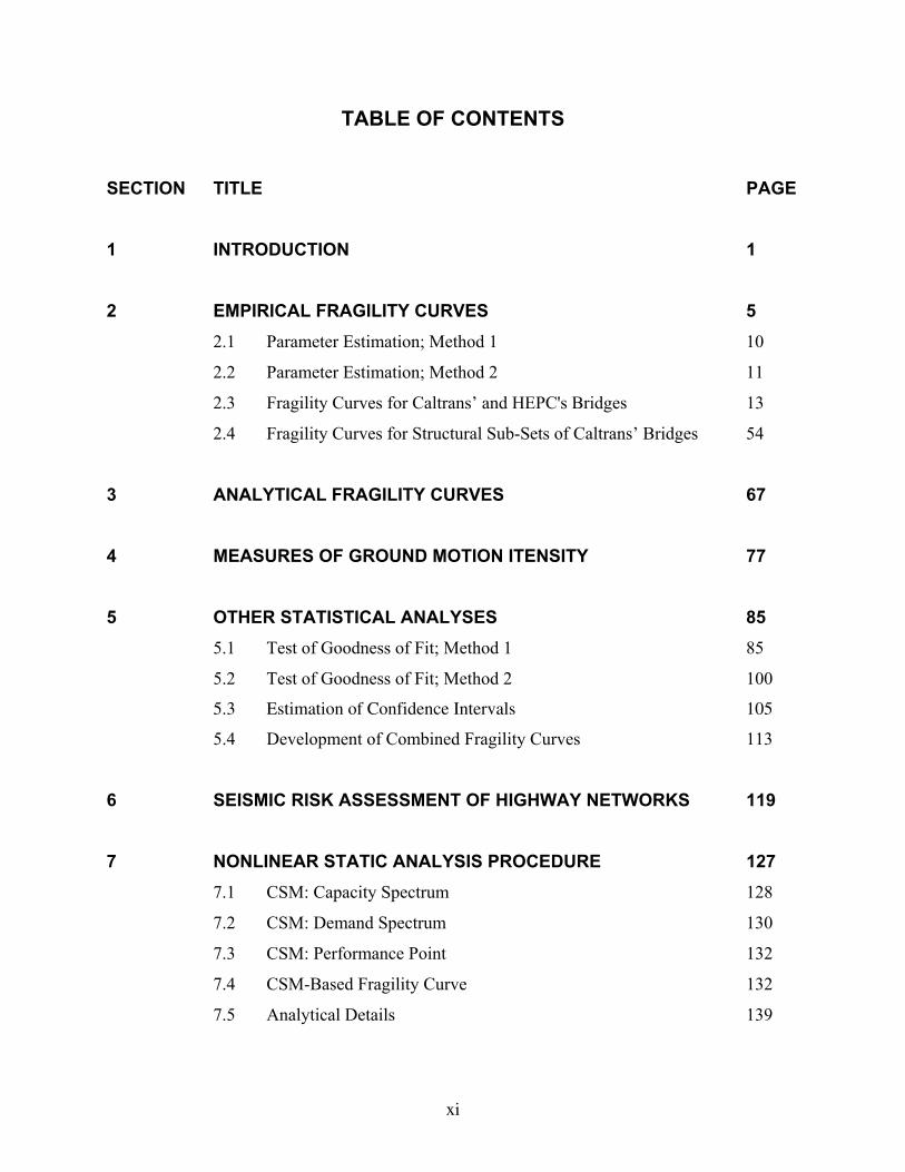
TABLE OF CONTENTS
SECTION TITLE PAGE
1 INTRODUCTION 1 2 EMPIRICAL FRAGILITY CURVES 5
2.1 Parameter Estimation; Method 1 10
2.2 Parameter Estimation; Method 2 11
2.3 Fragility Curves for Caltrans’ and HEPC's Bridges 13
2.4 Fragility Curves for Structural Sub-Sets of Caltrans’ Bridges 54
3 ANALYTICAL FRAGILITY CURVES 67 4 MEASURES OF GROUND MOTION ITENSITY 77 5 OTHER STATISTICAL ANALYSES 85
5.1 Test of Goodness of Fit; Method 1 85
5.2 Test of Goodness of Fit; Method 2 100
5.3 Estimation of Confidence Intervals 105
5.4 Development of Combined Fragility Curves 113
6 SEISMIC RISK ASSESSMENT OF HIGHWAY NETWORKS 119 7 NONLINEAR STATIC ANALYSIS PROCEDURE 127
7.1 CSM: Capacity Spectrum 128
7.2 CSM: Demand Spectrum 130
7.3 CSM: Performance Point 132
7.4 CSM-Based Fragility Curve 132
7.5 Analytical Details 139

xii
TABLE OF CONTENTS (cont’d)
SECTION TITLE PAGE
8 CONCLUSINONS 145 9 REFERENCES 147

xiii
LIST OF ILLUSTRATIONS
FIGURE TITLE PAGE
2-1 Description of States of Damage
for Hansin Expressway Cooperation's Bridge Columns 7
2-2 Schematics of Fragility Curves 13
2-3 Fragility Curves for Caltrans' Bridges (Method 1) 15
2-4 Fragility Curves for Caltrans' Bridges (Method 2) 16
2-5 Caltrans' Express Bridge Map in Los Angeles County 16
2-6 PGA Contour Map (1994 Northridge Earthquake; D. Wald) 17
2-7 Fragility Curve for Caltrans' Bridges
with at least Minor Damage and Input Damage Data (Method 1) 17
2-8 Fragility Curve for Caltrans' Bridges
with at least Moderate Damage and Input Damage Data (Method 1) 18
2-9 Fragility Curve for Caltrans' Bridges
with at least Major Damage and Input Damage Data (Method 1) 18
2-10 Fragility Curve for Caltrans' Bridges
with Collapse Damage and Input Damage Data (Method 1) 19
2-11 Fragility Curve for Caltrans' Bridges
with at least Minor Damage and Input Damage Data (Method 2) 19
2-12 Fragility Curve for Caltrans' Bridges
with at least Moderate Damage and Input Damage Data (Method 2) 20
2-13 Fragility Curve for Caltrans' Bridges
with at least Major Damage and Input Damage Data (Method 2) 20
2-14 Fragility Curve for Caltrans' Bridges
with Collapse Damage and Input Damage Data (Method 2) 21
2-15 A Typical Cross-Section of HEPC's Bridge Columns 21
2-16 Fragility Curves for HEPC's Bridge Columns (Method 1) 22
2-17 Fragility Curves for HEPC's Bridge Columns (Method 2) 22
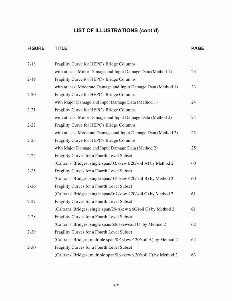
xiv
LIST OF ILLUSTRATIONS (cont’d)
FIGURE TITLE PAGE
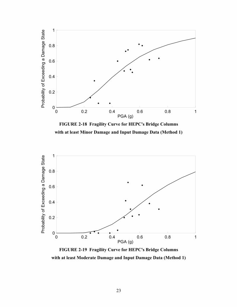
2-18 Fragility Curve for HEPC's Bridge Columns
with at least Minor Damage and Input Damage Data (Method 1) 23
2-19 Fragility Curve for HEPC's Bridge Columns
with at least Moderate Damage and Input Damage Data (Method 1) 23
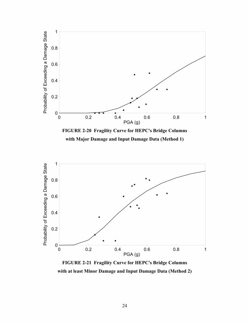
2-20 Fragility Curve for HEPC's Bridge Columns
with Major Damage and Input Damage Data (Method 1) 24
2-21 Fragility Curve for HEPC's Bridge Columns
with at least Minor Damage and Input Damage Data (Method 2) 24
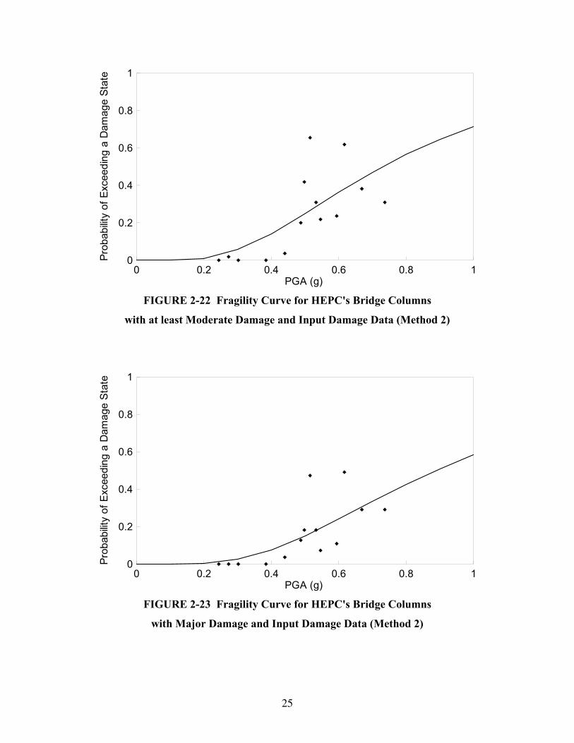
2-22 Fragility Curve for HEPC's Bridge Columns
with at least Moderate Damage and Input Damage Data (Method 2) 25
2-23 Fragility Curve for HEPC's Bridge Columns
with Major Damage and Input Damage Data (Method 2) 25
2-24 Fragility Curves for a Fourth Level Subset
(Caltrans' Bridges; single span/0 ≤ skew ≤ 20/soil A) by Method 2 60
2-25 Fragility Curves for a Fourth Level Subset
(Caltrans' Bridges; single span/0 ≤ skew ≤ 20/soil B) by Method 2 60
2-26 Fragility Curves for a Fourth Level Subset
(Caltrans' Bridges; single span/0 ≤ skew ≤ 20/soil C) by Method 2 61
2-27 Fragility Curves for a Fourth Level Subset
(Caltrans' Bridges; single span/20<skew ≤ 60/soil C) by Method 2 61
2-28 Fragility Curves for a Fourth Level Subset
(Caltrans' Bridges; single span/60<skew/soil C) by Method 2 62
2-29 Fragility Curves for a Fourth Level Subset
(Caltrans' Bridges; multiple span/0 ≤ skew ≤ 20/soil A) by Method 2 62
2-30 Fragility Curves for a Fourth Level Subset
(Caltrans' Bridges; multiple span/0 ≤ skew ≤ 20/soil C) by Method 2 63

xv
LIST OF ILLUSTRATIONS (cont’d)
FIGURE TITLE PAGE
2-31 Fragility Curves for a Fourth Level Subset
(Caltrans' Bridges; multiple span/20<skew ≤ 60/soil A) by Method 2 63
2-32 Fragility Curves for a Fourth Level Subset
(Caltrans' Bridges; multiple span/20<skew ≤ 60/soil B) by Method 2 64
2-33 Fragility Curves for a Fourth Level Subset
(Caltrans' Bridges; multiple span/20<skew ≤ 60/soil C) by Method 2 64
2-34 Fragility Curves for a Fourth Level Subset
(Caltrans' Bridges; multiple span/60<skew/soil A) by Method 2 65
2-35 Fragility Curves for a Fourth Level Subset
(Caltrans' Bridges; multiple span/60<skew/soil B) by Method 2 65
2-36 Fragility Curves for a Fourth Level Subset
(Caltrans' Bridges; multiple span/60<skew/soil C) by Method 2 66
2-37 Fragility Curves for Second Subset of Single Span Bridges 66
3-1 A Representative Memphis Bridge 71
3-2 New Madrid Seismic Zone and Marked Tree, AR 72
3-3 Typical Ground Acceleration Time Histories in the Memphis Area 72
3-4 Average Spectral Accelerations in the Memphis Area 73
3-5 Fragility Curves for Memphis Bridges 1 and 2 73
3-6 Fragility Curve for Bridge 1 with Major Damage and Input Damage Data 74
3-7 Fragility Curve for Bridge 1
with at least Minor Damage and Input Damage Data 74
3-8 Comparison of Fragility Curves
based on Sample Size 80 and 60 (Bridge 1 with at least Minor Damage) 75
3-9 Comparison of Fragility Curves
based on Sample Size 80 and 60 (Bridge 1 with Major Damage) 75
xvi
LIST OF ILLUSTRATIONS (cont’d)
FIGURE TITLE PAGE
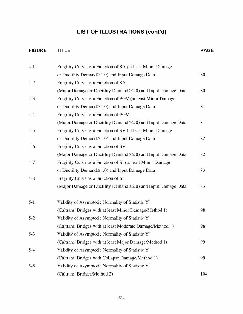
4-1 Fragility Curve as a Function of SA (at least Minor Damage
or Ductility Demand ≥ 1.0) and Input Damage Data 80
4-2 Fragility Curve as a Function of SA
(Major Damage or Ductility Demand ≥ 2.0) and Input Damage Data 80
4-3 Fragility Curve as a Function of PGV (at least Minor Damage
or Ductility Demand ≥ 1.0) and Input Damage Data 81
4-4 Fragility Curve as a Function of PGV
(Major Damage or Ductility Demand ≥ 2.0) and Input Damage Data 81
4-5 Fragility Curve as a Function of SV (at least Minor Damage
or Ductility Demand ≥ 1.0) and Input Damage Data 82
4-6 Fragility Curve as a Function of SV
(Major Damage or Ductility Demand ≥ 2.0) and Input Damage Data 82
4-7 Fragility Curve as a Function of SI (at least Minor Damage
or Ductility Demand ≥ 1.0) and Input Damage Data 83
4-8 Fragility Curve as a Function of SI
(Major Damage or Ductility Demand ≥ 2.0) and Input Damage Data 83
5-1 Validity of Asymptotic Normality of Statistic Y2
(Caltrans' Bridges with at least Minor Damage/Method 1) 98
5-2 Validity of Asymptotic Normality of Statistic Y2
(Caltrans' Bridges with at least Moderate Damage/Method 1) 98
5-3 Validity of Asymptotic Normality of Statistic Y2
(Caltrans' Bridges with at least Major Damage/Method 1) 99
5-4 Validity of Asymptotic Normality of Statistic Y2
(Caltrans' Bridges with Collapse Damage/Method 1) 99
5-5 Validity of Asymptotic Normality of Statistic Y2
(Caltrans' Bridges/Method 2) 104
xvii
LIST OF ILLUSTRATIONS (cont’d)
FIGURE TITLE PAGE
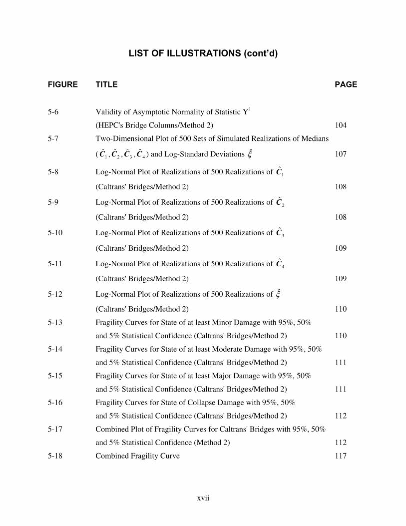
5-6 Validity of Asymptotic Normality of Statistic Y2
(HEPC's Bridge Columns/Method 2) 104
5-7 Two-Dimensional Plot of 500 Sets of Simulated Realizations of Medians
( 1C , 2C , 3C , 4C ) and Log-Standard Deviations ξ 107
5-8 Log-Normal Plot of Realizations of 500 Realizations of 1C
(Caltrans' Bridges/Method 2) 108
5-9 Log-Normal Plot of Realizations of 500 Realizations of 2C
(Caltrans' Bridges/Method 2) 108
5-10 Log-Normal Plot of Realizations of 500 Realizations of 3C
(Caltrans' Bridges/Method 2) 109
5-11 Log-Normal Plot of Realizations of 500 Realizations of 4C
(Caltrans' Bridges/Method 2) 109
5-12 Log-Normal Plot of Realizations of 500 Realizations of ξ
(Caltrans' Bridges/Method 2) 110
5-13 Fragility Curves for State of at least Minor Damage with 95%, 50%
and 5% Statistical Confidence (Caltrans' Bridges/Method 2) 110
5-14 Fragility Curves for State of at least Moderate Damage with 95%, 50%
and 5% Statistical Confidence (Caltrans' Bridges/Method 2) 111
5-15 Fragility Curves for State of at least Major Damage with 95%, 50%
and 5% Statistical Confidence (Caltrans' Bridges/Method 2) 111
5-16 Fragility Curves for State of Collapse Damage with 95%, 50%
and 5% Statistical Confidence (Caltrans' Bridges/Method 2) 112
5-17 Combined Plot of Fragility Curves for Caltrans' Bridges with 95%, 50%
and 5% Statistical Confidence (Method 2) 112
5-18 Combined Fragility Curve 117
xviii
LIST OF ILLUSTRATIONS (cont’d)
FIGURE TITLE PAGE
6-1 Los Angeles Areas Highway Network 122
6-2 Location Map of Bridges with Major Damage 123
6-3 Simulated Network Damage under Postulated Elysian Park Earthquake 124
6-4 Averaged Network Damage under Postulated Elysian Park Earthquake
(10 Simulations) 124
6-5 Averaged Network Damage under Postulated Elysian Park Earthquake (10
Simulations on retrofitted Network with Fragility Enhancement of 50%) 125
7-1 Capacity Spectra 130
7-2 Mean, Mean+1Sigma and Mean-1Sigma ADRS for PGA=0.25g 135
7-3 Mean, Mean+1Sigma and Mean-1Sigma ADRS for PGA=0.40g 135
7-4 Calculated Performance Displacement for Mean ADRS for PGA=0.25g 136
7-5 Calculated Performance Displacement for Mean+1Sigma ADRS
for PGA=0.25g 136
7-6 Calculated Performance Displacement for Mean-1Sigma ADRS
for PGA=0.25g 137
7-7 Fragility Curves of 10 Sample Bridges for State of at least Minor Damage 137
7-8 Fragility Curves of 10 Sample Bridges for State of Major Damage 138
7-9 Average Acceleration Response Spectra (5% Damping) 138
7-10 Average Pseudo Velocity Response Spectrum (5% Damping) 141
7-11 Average Pseudo Displacement Response Spectrum (5% Damping) 142
7-12 Fundamental Natural Periods of 10 Sample Bridges 142
7-13 Mean, Mean+1Sigma and Mean-1Sigma Displacement
for One Sample Bridge 143
xix
LIST OF TABLES
TABLE TITLE PAGE 2-1 Northridge Earthquake Damage Data 6
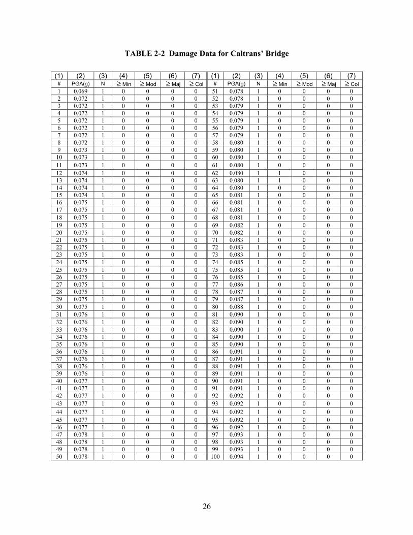
2-2 Damage Data for Caltrans' Bridges 26
2-3 Damage Data for HEPC's Bridge Columns 46
2-4 Median and Log-Standard Deviation
at different Levels of Sample Sub-Division 57
5-1 2yP Values for Goodness of Fit (Method 1) 88
5-2(a) Work-Sheet for Test of Goodness of Fit
(Minor Damage/Caltrans' Bridges/Method 1) 89
5-2(b) Work-Sheet for Test of Goodness of Fit
(Moderate Damage/Caltrans' Bridges/Method 1) 90
5-2(c) Work-Sheet for Test of Goodness of Fit
(Major Damage/Caltrans' Bridges/Method 1) 91
5-2(d) Work-Sheet for Test of Goodness of Fit
(Collapse Damage/Caltrans' Bridges/Method 1) 92
5-3(a) Work-Sheet for Test of Goodness of Fit
(Minor Damage/HEPC's Bridges/Method 1) 93
5-3(b) Work-Sheet for Test of Goodness of Fit
(Moderate Damage/HEPC's Bridges/Method 1) 93
5-3(c) Work-Sheet for Test of Goodness of Fit
(Major Damage/HEPC's Bridges/Method 1) 93
5-4(a) Work-Sheet for Test of Goodness of Fit
(Minor Damage/Memphis Bridge 1/Method 1) 94
5-4(b) Work-Sheet for Test of Goodness of Fit
(Major Damage/Memphis Bridge 1/Method 1) 95
xx
LIST OF TABLES (cont’d)
TABLE TITLE PAGE 5-5(a) Work-Sheet for Test of Goodness of Fit
(Minor Damage/Memphis Bridge 2/Method 1) 96
5-5(b) Work-Sheet for Test of Goodness of Fit
(Major Damage/Memphis Bridge 2/Method 1) 97
5-6 Work-Sheet for Test of Goodness of Fit
(Caltrans' Bridges/Method 2) 102
5-7 Work-Sheet for Test of Goodness of Fit
(HEPC's Bridge Columns/ Method 2) 103
6-1 Bridge and Link Damage Index and Traffic Flow Capacity 120
7-1 Minimum allowable ASR and VSR Values (ATC 1996) 131
7-2 Values for Damping Modification Factor, κ (ATC 1996) 131

1
SECTION 1 INTRODUCTION
Bridges are potentially one of the most seismically vulnerable structures in the highway system.
While performing a seismic risk analysis of a highway system, it is imperative to identify seismic
vulnerability of bridges associated with various states of damage. The development of
vulnerability information in the form of fragility curves is a widely practiced approach when the
information is to be developed accounting for a multitude of uncertain sources involved, for
example, in estimation of seismic hazard, structural characteristics, soil-structure interaction, and
site conditions.
In principle, the development of bridge fragility curves will require synergistic use of the
following methods: (1) professional judgement, (2) quasi-static and design code consistent
analysis, (3) utilization of damage data associated with past earthquakes, and (4) numerical
simulation of bridge seismic response based on structural dynamics.
An exploratory work is carried out in this study to develop fragility curves for comparison
purposes on the basis of the nonlinear static method consistent with method (2) in the preceding
paragraph. The major effort of this study, however, is placed on the development of empirical
and analytical fragility curves as described in methods (3) and (4) above, respectively: the former
by utilizing the damage data associated with past earthquakes, and the latter by numerically
simulating seismic response with the aid of structural dynamic analysis. At the same time, it
introduces statistical procedures appropriate for the development of fragility curves under the
assumption that they can be represented by two-parameter lognormal distribution functions with
the unknown median and log-standard deviation. These two-parameters are referred to as the
fragility parameters in this study. Two different sets of procedures describe how the fragility
parameters are estimated, the test of goodness of fit can be performed and confidence intervals of
the parameters estimated. The one procedure (Method 1) is used when the fragility curves are
independently developed for different states of damage, while the other (Method 2) when they
are constructed dependently on each other in such a way that the log-standard deviation is

2
common to all the fragility curves. The empirical fragility curves are developed utilizing bridge
damage data obtained from the past earthquakes, particularly the 1994 Northridge and the 1995
Hyogo-ken Nanbu (Kobe) earthquake. Analytical fragility curves are developed for typical
bridges in the Memphis, Tennessee area on the basis of a nonlinear dynamic analysis.
Two-parameter lognormal distribution functions were traditionally used for fragility curve
construction. This was motivated by its mathematical expedience in approximately relating the
actual structural strength capacity with the design strength through an overall factor of safety
which can be assumedly factored into a number of multiplicative safety factors, each associated
with a specific source of uncertainty. When the lognormal assumption is made for each of these
factors, the overall safety factor also distributes lognormally due to the multiplicative
reproducibility of the lognormal variables. This indeed was the underpinning assumption that
was made in the development of probabilistic risk assessment methodology for nuclear power
plants in the 1970’s and in the early 1980’s (NRC, 1983). Although this assumption is not
explicitly used in this report, fragility curves are modeled by lognormal distribution function in
this study. Use of the three-parameter lognormal distribution functions for fragility curves is
possible with the third parameter estimating the threshold of ground motion intensity below
which the structure will never sustain any damage. However, this has never been a popular
decision primarily because no one wishes to make such a definite, potentially unconservative
assumption.
The study also includes the sections where some preliminary evaluations are made on the
significance of the fragility curves developed as a function of ground intensity measures other
than PGA, and furthermore, applications of fragility curves in the seismic performance
estimation of expressway network systems are demonstrated.
Finally, an exploratory work is performed to compare the analytical fragility curves developed in
the major part of this study with those constructed utilizing the nonlinear static method currently
promoted by the profession in conjunction with performance-based structural design.
The conceptual and theoretical treatment dealt with in this study is believed to provide a
theoretical basis and analytical tools of practical usefulness for the development of fragility

3
curves and their applications in the assessment of seismic performance of expressway network
systems.
This study emphasizes statistical analysis of fragility curves and in that sense it is rather unique
together with Basoz and Kiremidjian (1998). The reader is referred to the following papers,
among many others, for the previous work performed on fragility curves with different emphasis
and developed for civil structures; ATC-13 (ATC, 1985), Barron-Corvera (1999), Dutta and
Mander (1998), Hwang et al. (1997), Hwang amd Huo (1998), Hwang et al. (1999), Nakamura
and Mizutani (1996), Nakamura et al. (1998), Shinozuka et al. (1999), and Singhal and
Kiremidjian (1997).


5
SECTION 2 EMPIRICAL FRAGILITY CURVES
It is assumed that the empirical fragility curves can be expressed in the form of two-parameter
lognormal distribution functions, and developed as functions of peak ground acceleration (PGA)
representing the intensity of the seismic ground motion. Use of PGA for this purpose is
considered reasonable since it is not feasible to evaluate spectral acceleration by identifying
significantly participating natural modes of vibration for each of the large number of bridges
considered for the analysis here, without having a corresponding reliable ground motion time
history. The PGA value at each bridge location is determined by interpolation and extrapolation
from the PGA data due to D. Wald of USGS (Wald, 1998).
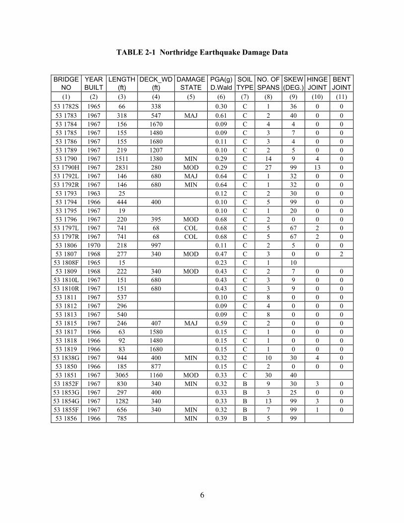
For the development of empirical fragility curves, the damage reports are usually utilized to
establish the relationship between the ground motion intensity and the damage state of each
bridge. This is also the case for the present study. One typical page of the damage report for the
Caltrans’ bridges under the Northridge event is shown in table 2-1, where the extent of damage is
classified in column 5 into the state of no, minor, moderate and major damage in addition to the
state of collapse. The report did not provide explicit physical definitions of these damage states
(in column 5, a blank space signifies no damage). As far as the Caltrans’ bridges are concerned,
this inspection report (table 2-1) is used when a damage state is assigned to each bridge in the
analysis that follows. In view of the time constraint in which the inspection had to be completed
after the earthquake, the classification of each bridge into one of the five damage states,
understandably, contains some elements of judgement.
Hanshin Expressway Public Corporation’s (HEPC’s) report on the damage sustained by RC
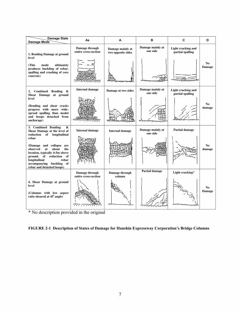
bridge columns resulting from the Kobe earthquake uses five classes of damage state as shown in
figure 2-1 in which the damage states As, A, B, C and D are defined by the corresponding
sketches of damage within each of four failure modes. It appears reasonable to consider that
these damage states are respectively classified as states of collapse (As), major damage (A),
moderate damage (B), minor damage (C) and no damage (D).
6
TABLE 2-1 Northridge Earthquake Damage Data
BRIDGE YEAR LENGTH DECK_WD DAMAGE PGA(g) SOIL NO. OF SKEW HINGE BENTNO BUILT (ft) (ft) STATE D.Wald TYPE SPANS (DEG.) JOINT JOINT(1) (2) (3) (4) (5) (6) (7) (8) (9) (10) (11)
53 1782S 1965 66 338 0.30 C 1 36 0 0 53 1783 1967 318 547 MAJ 0.61 C 2 40 0 0 53 1784 1967 156 1670 0.09 C 4 4 0 0 53 1785 1967 155 1480 0.09 C 3 7 0 0 53 1786 1967 155 1680 0.11 C 3 4 0 0 53 1789 1967 219 1207 0.10 C 2 5 0 0 53 1790 1967 1511 1380 MIN 0.29 C 14 9 4 0
53 1790H 1967 2831 280 MOD 0.29 C 27 99 13 0 53 1792L 1967 146 680 MAJ 0.64 C 1 32 0 0 53 1792R 1967 146 680 MIN 0.64 C 1 32 0 0 53 1793 1963 25 0.12 C 2 30 0 0 53 1794 1966 444 400 0.10 C 5 99 0 0 53 1795 1967 19 0.10 C 1 20 0 0 53 1796 1967 220 395 MOD 0.68 C 2 0 0 0
53 1797L 1967 741 68 COL 0.68 C 5 67 2 0 53 1797R 1967 741 68 COL 0.68 C 5 67 2 0 53 1806 1970 218 997 0.11 C 2 5 0 0 53 1807 1968 277 340 MOD 0.47 C 3 0 0 2
53 1808F 1965 15 0.23 C 1 10 53 1809 1968 222 340 MOD 0.43 C 2 7 0 0
53 1810L 1967 151 680 0.43 C 3 9 0 0 53 1810R 1967 151 680 0.43 C 3 9 0 0 53 1811 1967 537 0.10 C 8 0 0 0 53 1812 1967 296 0.09 C 4 0 0 0 53 1813 1967 540 0.09 C 8 0 0 0 53 1815 1967 246 407 MAJ 0.59 C 2 0 0 0 53 1817 1966 63 1580 0.15 C 1 0 0 0 53 1818 1966 92 1480 0.15 C 1 0 0 0 53 1819 1966 83 1680 0.15 C 1 0 0 0
53 1838G 1967 944 400 MIN 0.32 C 10 30 4 0 53 1850 1966 185 877 0.15 C 2 0 0 0 53 1851 1967 3065 1160 MOD 0.33 C 30 40
53 1852F 1967 830 340 MIN 0.32 B 9 30 3 0 53 1853G 1967 297 400 0.33 B 3 25 0 0 53 1854G 1967 1282 340 0.33 B 13 99 3 0 53 1855F 1967 656 340 MIN 0.32 B 7 99 1 0 53 1856 1966 785 MIN 0.39 B 5 99
7
Damage State Damage Mode As A B C D
1. Bending Damage at ground level (This mode ultimately produces buckling of rebar, spalling and crushing of core concrete)
Damage through entire cross-section
Damage mainly at two opposite sides
Damage mainly at one side
Light cracking and partial spalling
No Damage
2. Combined Bending & Shear Damage at ground level (Bending and shear cracks progress with more wide-spread spalling than model and hoops detached from anchorage)
Internal damage
Damage at two sides
Damage mainly at one side
Light cracking and partial spalling
No damage
3. Combined Bending & Shear Damage at the level of reduction of longitudinal rebar (Damage and collapse are observed at about the location, typically 4-5m above ground, of reduction of longitudinal rebar accompanying buckling of rebar and detached hoops)
Internal damage
Internal damage
Damage mainly at one side
Partial damage
No damage
4. Shear Damage at ground level (Columns with low aspect ratio sheared at 450 angle)
Damage through entire cross-section
Damage through column
Partial damage
Light cracking*
No Damage
* No description provided in the original
FIGURE 2-1 Description of States of Damage for Hanshin Expressway Corporation’s Bridge Columns
8
The perishable nature of damage information urgently calls for the establishment of standardized
description of seismic damage based on more physical interpretation of what is visual for the
post-earthquake damage inspection in the future destructive earthquake. Such description of
seismic damage carefully recorded will be of lasting value to the earthquake engineering
research community for the development of its capability in systematically estimating the
seismic vulnerability of urban built environment. In this respect, classification more rigorously
defined on the basis of quantitative analysis of physical damage is highly desirable. This,
however, was not pursued in this study for various practical reasons; one dominant reason is the
anticipated difficulty in collecting and interpreting detailed damage data that would permit such
a quantitative analysis. Obviously, the fragility curves developed in this study on the basis of
these damage data are valid for the Caltrans’ and HEPC’s bridges prior to the their repair and
retrofit that took place after the earthquakes. In this context, it is an interesting subject of future
study to examine the impact of repair and retrofit from the viewpoint of fragility curve
enhancement.
In this study, the parameter estimation, hypotheses testing and confidence interval estimation
related to the fragility curves are carried out in two different ways. The first method (Method 1)
independently develops a fragility curve for each of a damage state for each sample of bridges
with a given set of bridge attributes. A family of four fragility curves can, for example, be
developed independently for the damage states respectively identified as “at least minor”, “at
least moderate”, “at least major” and “collapse”, making use of the entire sample (of size equal
to 1,998) of Caltrans' expressway bridges in Los Angeles County, California subjected to the
Northridge earthquake and inspected for damage after the earthquake. This is done by
estimating, by the maximum likelihood method, the two fragility parameters of each lognormal
distribution function representing a fragility curve for a specific state of damage. These fragility
curves are valid under the assumption that the entire sample is statistically homogeneous. The
same independent estimation procedure can be applied to samples of bridges more realistically
categorized. A sample consisting only of single span bridges out of the entire sample is such a
case for which four fragility curves can also be independently developed for all the bridges with
a single span. Method 1 also includes the procedure to test the hypothesis that the observed
9
damage data are generated by chance from the corresponding fragility curves thus developed
(test of goodness of fit). In addition, Method 1 provides a procedure of estimating statistical
confidence intervals of the fragility parameters through a Monte Carlo simulation technique.
It is noted that the bridges in a state of damage as defined above include a sub-set of the bridges
in a severer state of damage implying that the fragility curves developed for different states of
damage within a sample are not supposed to intersect. Intersection of fragility curves can
happen, however, under the assumption that they are all represented by lognormal distribution
functions and constructed independently, unless log-standard derivations are identical for all the
fragility curves. This observation leads to the following method referred to as Method 2, where
the parameters of the lognormal distribution functions representing different states of damage are
simultaneously estimated by means of the maximum likelihood method. In this method, the
parameters to be estimated are the median of each fragility curve and one value of the log-
standard derivation prescribed to be common to all the fragility curves. The hypothesis testing
and confidence interval estimation will follow accordingly.
Additional comments are in order with respect to the assumption that all fragility curves are
represented by lognormal distributions. As mentioned above, bridges in a severer state of
damage constitute a sub-set of those in a state of lesser damage, and fragility curves associated
with the severer states must be determined taking into consideration that they are statistically
conditional to the fragility curves associated with the lesser states of severity. Hence, as the
common sense also dictates, the values of the fragility curve at a specified ground motion
intensity such as PGA is always larger for a lesser state of damage than that for a severer state.
Although the assumption of lognormal distribution functions with identical log-standard
deviation satisfies the requirement just mentioned, this is not sufficient to theoretically justify the
use of lognormal distribution functions for fragility curves associated with all states of damage.
In this regard, it is possible to develop a conditional fragility curve associated with each state of
damage. This is achieved by implementing the following three steps (Mizutani, 1999); first,
consider the (unconditional) fragility curve for a state of “at least minor” damage. Second,
develop the conditional fragility curve for bridges with a state of damage one rank severer, i.e.,
“at least moderate” damage. This conditional fragility curve is constructed for the bridges in a
10
state of “at least moderate” damage, considering only those bridges in the “at least minor” state
of damage. Finally, the conditional fragility value for the “at least moderate” state of damage is
multiplied by the unconditional fragility value for the “at least minor” state of damage at each
value of ground motion intensity to obtain the unconditional fragility curve for the “at least
moderate” state of damage. Sequentially applied, this three-step process will produce a family of
four fragility curves for “at least minor”, “at least moderate”, “at least major” and “collapse” (in
the case of Caltrans’ bridges considered in this study) which will not intersect. The fragility
curve for “at least minor” state of damage is unconditional to begin with since the state of
damage one rank less severe is the state of “at least no” damage which is satisfied by each and
every bridge of the entire sample of bridges.
While the three-step process above does produce a family of fragility curves that will not
intersect, it cannot always develop lognormal distribution functions for all the damage states
either independently or simultaneously. For mathematical expedience and computational ease,
this study uses Methods 1 and 2 to develop fragility curves in the form of lognormal distribution
function.
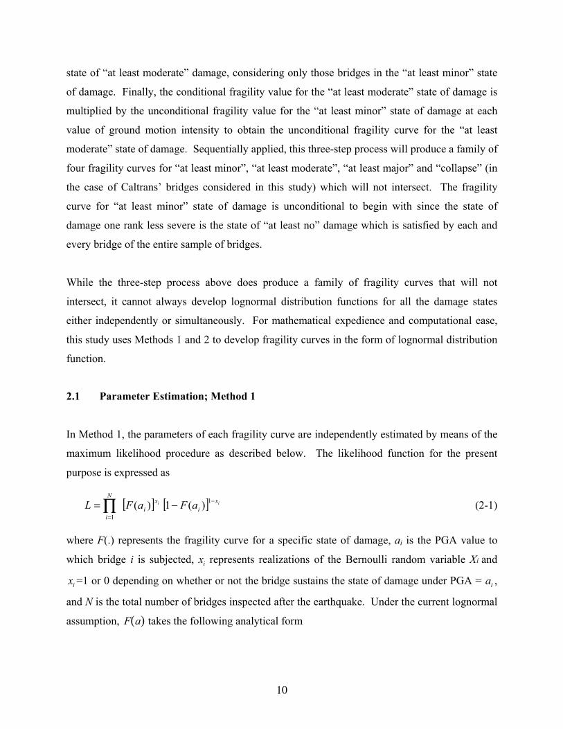
2.1 Parameter Estimation; Method 1
In Method 1, the parameters of each fragility curve are independently estimated by means of the
maximum likelihood procedure as described below. The likelihood function for the present
purpose is expressed as
[ ] [ ] ii xi
xi
N
i
aFaFL −
=
−= ∏ 1
1
)(1 )( (2-1)
where F(.) represents the fragility curve for a specific state of damage, ai is the PGA value to
which bridge i is subjected, xi represents realizations of the Bernoulli random variable Xi and
xi =1 or 0 depending on whether or not the bridge sustains the state of damage under PGA = ai ,
and N is the total number of bridges inspected after the earthquake. Under the current lognormal
assumption, F a( ) takes the following analytical form
11
( )
Φ=ζ
ca
aFln (2-2)
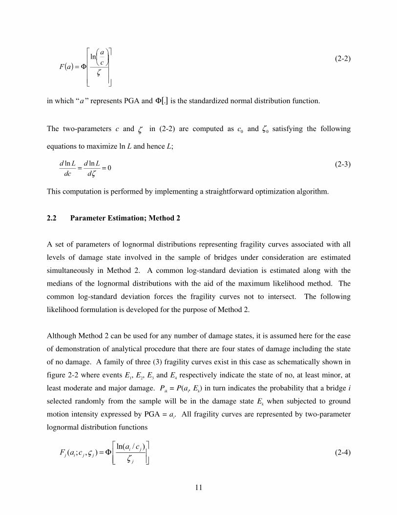
in which “a ” represents PGA and Φ .[] is the standardized normal distribution function.
The two-parameters c and ζ in (2-2) are computed as c0 and ζ 0 satisfying the following
equations to maximize ln L and hence L;
0lnln ==ζd
Lddc
Ld (2-3)
This computation is performed by implementing a straightforward optimization algorithm.
2.2 Parameter Estimation; Method 2
A set of parameters of lognormal distributions representing fragility curves associated with all
levels of damage state involved in the sample of bridges under consideration are estimated
simultaneously in Method 2. A common log-standard deviation is estimated along with the
medians of the lognormal distributions with the aid of the maximum likelihood method. The
common log-standard deviation forces the fragility curves not to intersect. The following
likelihood formulation is developed for the purpose of Method 2.
Although Method 2 can be used for any number of damage states, it is assumed here for the ease
of demonstration of analytical procedure that there are four states of damage including the state
of no damage. A family of three (3) fragility curves exist in this case as schematically shown in
figure 2-2 where events E1, E2, E3 and E4 respectively indicate the state of no, at least minor, at
least moderate and major damage. Pik = P(ai, Ek) in turn indicates the probability that a bridge i
selected randomly from the sample will be in the damage state Ek when subjected to ground
motion intensity expressed by PGA = ai. All fragility curves are represented by two-parameter
lognormal distribution functions
ln( / )( ; , ) i j
j i j jj
a cF a c ς
ζ
= Φ
(2-4)
12
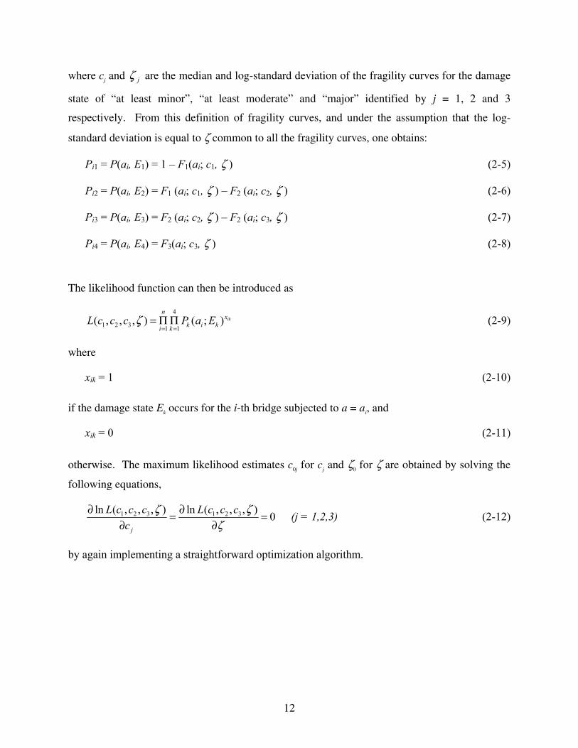
where cj and jζ are the median and log-standard deviation of the fragility curves for the damage
state of “at least minor”, “at least moderate” and “major” identified by j = 1, 2 and 3
respectively. From this definition of fragility curves, and under the assumption that the log-
standard deviation is equal to ζ common to all the fragility curves, one obtains:
Pi1 = P(ai, E1) = 1 – F1(ai; c1, ζ ) (2-5)
Pi2 = P(ai, E2) = F1 (ai; c1, ζ ) – F2 (ai; c2, ζ ) (2-6)
Pi3 = P(ai, E3) = F2 (ai; c2, ζ ) – F2 (ai; c3, ζ ) (2-7)
Pi4 = P(ai, E4) = F3(ai; c3, ζ ) (2-8)
The likelihood function can then be introduced as
4
1 2 3 1 1( , , , ) ( ; ) ik
nx
k i ki kL c c c P a Eζ
= == Π Π (2-9)
where
xik = 1 (2-10)
if the damage state Ek occurs for the i-th bridge subjected to a = ai, and
xik = 0 (2-11)
otherwise. The maximum likelihood estimates c0j for cj and ζ0 for ζ are obtained by solving the
following equations,
1 2 3 1 2 3ln ( , , , ) ln ( , , , ) 0j
L c c c L c c cc
ζ ζζ
∂ ∂= =∂ ∂
(j = 1,2,3) (2-12)
by again implementing a straightforward optimization algorithm.
13
0 0.2 0.4 0.6 0.8 1 1.2 1.4PGA (g)
0
0.2
0.4
0.6
0.8
1
Prob
abilit
y of
Exc
eedi
ng a
Dam
age
Stat
eP(E )
P(E )
P(E )
P(E )
FIGURE 2-2 Schematics of Fragility Curves
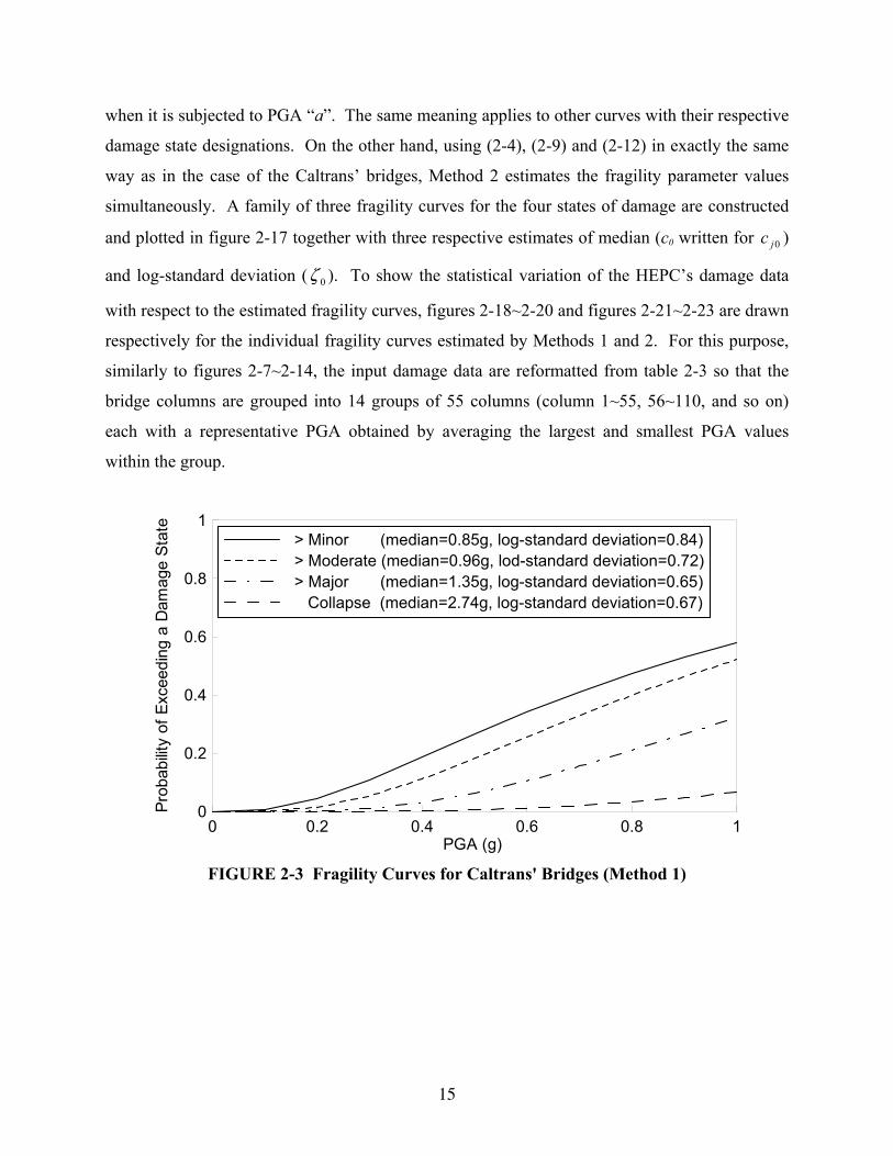
2.3 Fragility curves for Caltrans’ and HEPC's bridges
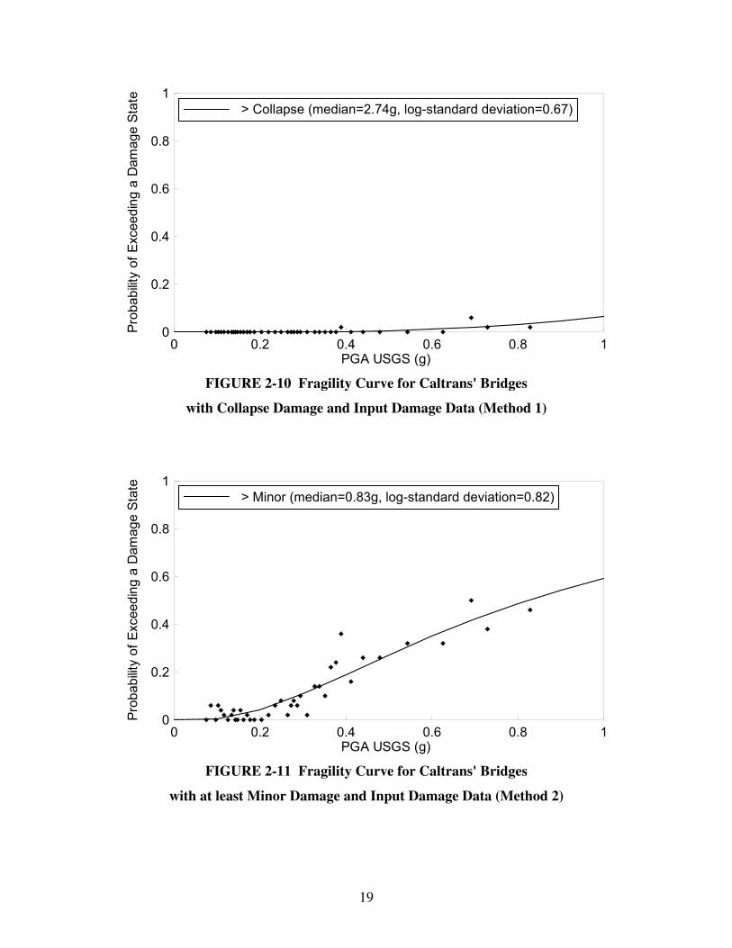
Four fragility curves for Caltrans’ bridges associated with the four states of damages are plotted
in figures 2-3 and 2-4, upon estimating the parameters involved by Methods 1 and 2 respectively
(with their respective median and log-standard deviation values also indicated). These fragility
curves are constructed on the damage data summarized in the format of table 2-2 which, for
computational convenience, is transformed from that of table 2-1 which is developed in principle
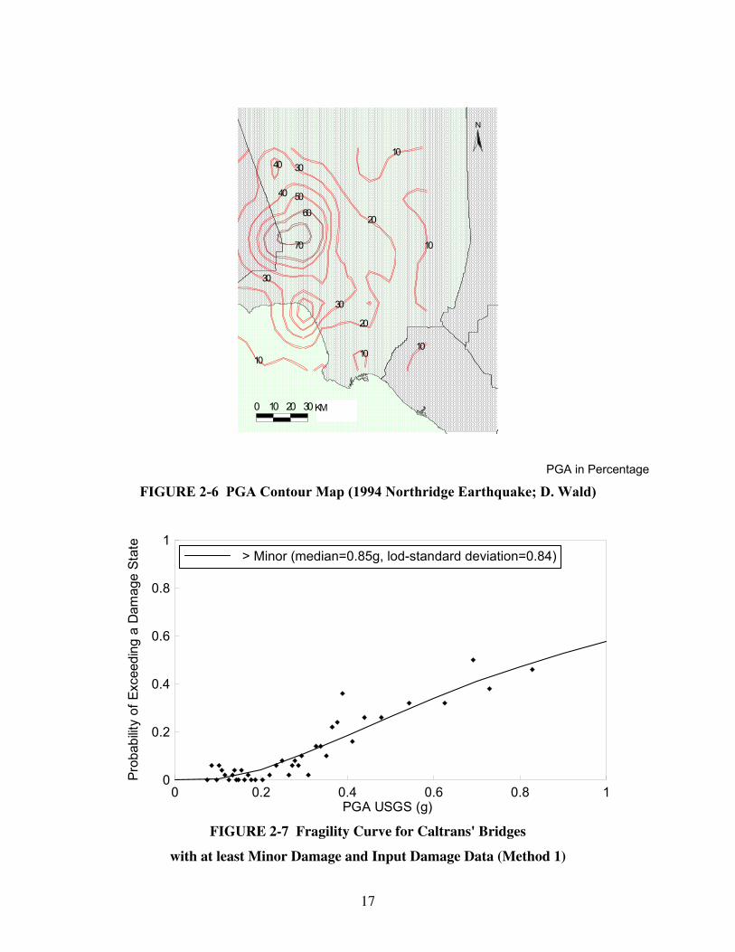
by overlaying the Caltrans’ bridge map (figure 2-5) on the Northridge earthquake PGA contour
map due to D. Wald (figure 2-6). In table 2-2, bridges are renumbered in the ascending order
with respect to PGA. The entry of 1 in each of the columns (4)~(7) indicates that the bridge is at
least in the state of damage designated by the column, while the entry of 0 shows that the bridge
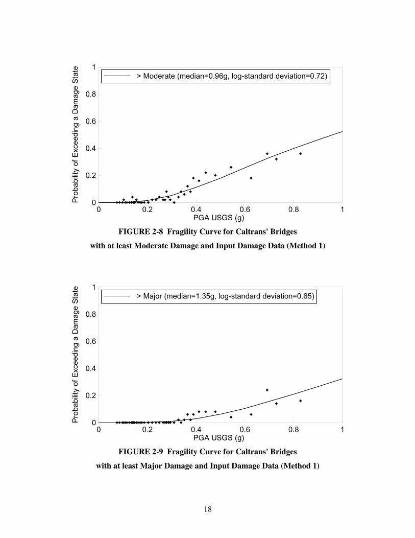
does not suffer from the state of damage designated or severer. Figures 2-7~2-10 show
separately the four fragility curves developed for Caltrans’ bridges obtained by Method 1 (figure
2-3) together with the damage data further transformed from table 2-2 just to demonstrate the
statistical variation of the data relative to the estimated fragility curve. The black diamonds in
figures 2-7~2-10 indicate these damage data developed in such a way that the entire sample of
1998 bridges are sub-divided into 44 groups of 44 bridges (starting from bridges 1~44, bridges
45~88, and so on) with the last group having 62 bridges. The number of the bridges that
14
sustained the state of damage under consideration in a group is divided by the total number of
bridges in the group (which is 44 except for the last group) and this ratio is used as a realization
of fragility value at the PGA value representative of the group obtained by averaging the smallest
and the largest PGA value assigned to the bridges in the group. Whether the fit of the fragility
curves to the input data can be judged acceptable in statistical sense is the subject of study in a
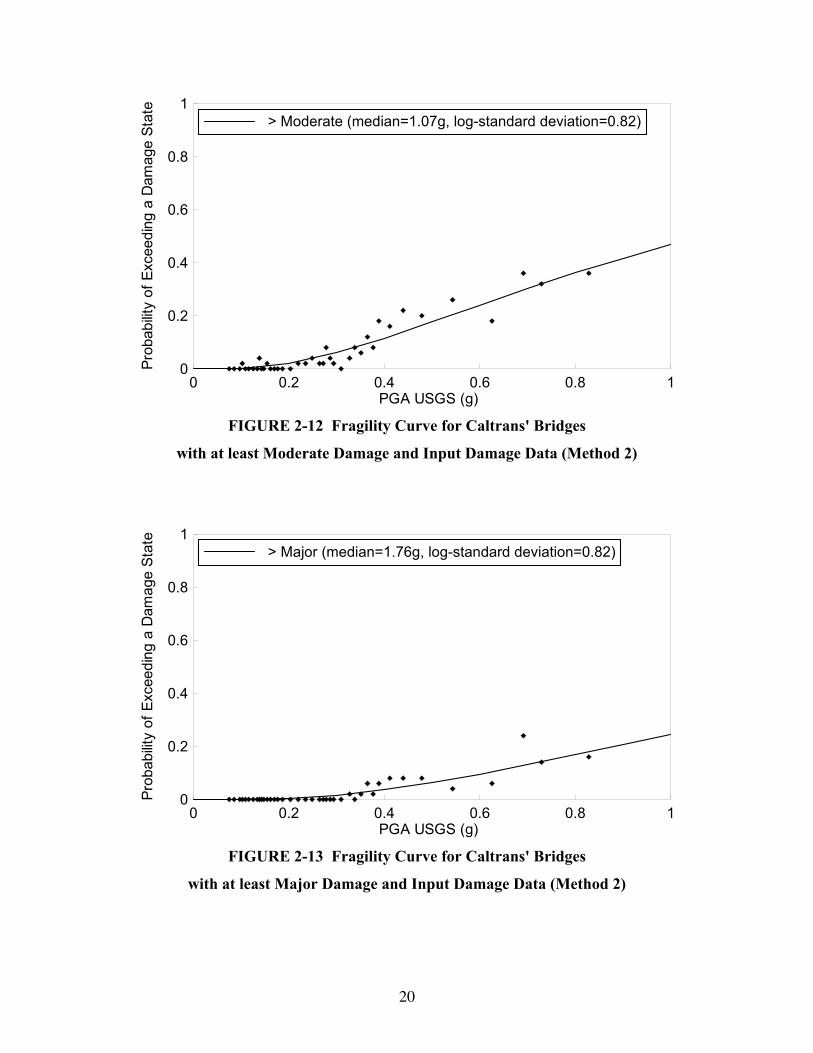
later section of this report (Section 5.1 and 5.2). Figures 2-11~2-14 show the statistical variation
of the same input data relative to the estimated fragility curves obtained by Method 2 (figure 2-4)
with each curve plotted separately (though estimated together). The fragility curves identified by
“minor” in figures 2-7 and 2-11 are associated with the state of “at least minor damage”. Similar
meaning applies to other three fragility curves identified by “moderate”, “major” and “collapse”,
unless specified otherwise. The difference between figures 2-3 and 2-4 is relatively
insignificant, although Method 2 produced larger probabilities of minor damage and smaller
probabilities of major damage than Method 1 throughout the range of PGA examined.
Fragility curves are also constructed (Nakamura et al., 1998) on the basis of a sample of 770
single-support reinforced concrete columns along two stretches of the viaduct, one in the HEPC's
Kobe Route and the other in the Ikeda Route with total length of approximately 40 km. Table 2-
3 represents the input damage data reformatted from the damage report by HEPC's engineers
after the 1995 Kobe earthquake. These bridge columns are of similar geometry and similarly
reinforced as shown in figure 2-15 which is drawn for a typical column (#Kou-P362). In this
respect, the 770 columns under consideration here constitute a much more homogeneous
statistical sample than the Caltrans' bridges considered earlier. The PGA value at each column
location under the Kobe earthquake is estimated by Nakamura et al (1998) on the basis of the
work by Nakamura et al (1996).
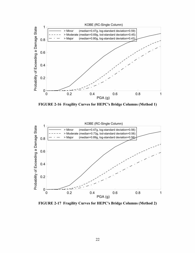
Integrating the damage state information with that of the PGA, and making use of the maximum
likelihood method involving (2-1)~(2-3), three (3) sets of 0c and 0ζ are obtained independently
by Method 1 and corresponding three fragility curves for the states of at least minor, at least
moderate and at least major damage are constructed as shown in figure 2-16 together with values
of the median c0 and log-standard deviation ζ 0 . As in the case of Caltrans' bridges, the curve
with “minor” designation represents, at each PGA value “a”, the probability that “at least minor”
state of damage will be sustained by a bridge (arbitrarily chosen from the sample of bridges)
15
when it is subjected to PGA “a”. The same meaning applies to other curves with their respective
damage state designations. On the other hand, using (2-4), (2-9) and (2-12) in exactly the same
way as in the case of the Caltrans’ bridges, Method 2 estimates the fragility parameter values
simultaneously. A family of three fragility curves for the four states of damage are constructed
and plotted in figure 2-17 together with three respective estimates of median (c0 written for 0jc )
and log-standard deviation ( 0ζ ). To show the statistical variation of the HEPC’s damage data
with respect to the estimated fragility curves, figures 2-18~2-20 and figures 2-21~2-23 are drawn
respectively for the individual fragility curves estimated by Methods 1 and 2. For this purpose,
similarly to figures 2-7~2-14, the input damage data are reformatted from table 2-3 so that the
bridge columns are grouped into 14 groups of 55 columns (column 1~55, 56~110, and so on)
each with a representative PGA obtained by averaging the largest and smallest PGA values
within the group.
0 0.2 0.4 0.6 0.8 1PGA (g)
0
0.2
0.4
0.6
0.8
1
Prob
abilit
y of
Exc
eedi
ng a
Dam
age
Stat
e
> Minor (median=0.85g, log-standard deviation=0.84) > Moderate (median=0.96g, lod-standard deviation=0.72) > Major (median=1.35g, log-standard deviation=0.65) Collapse (median=2.74g, log-standard deviation=0.67)
FIGURE 2-3 Fragility Curves for Caltrans' Bridges (Method 1)
16
0 0.2 0.4 0.6 0.8 1PGA (g)
0
0.2
0.4
0.6
0.8
1
Prob
abilit
y of
Exc
eedi
ng a
Dam
age
Stat
e
> Minor (median=0.83g, log-standard deviation=0.82) > Moderate (median=1.07g, lod-standard deviation=0.82) > Major (median=1.76g, log-standard deviation=0.82) Collapse (median=3.96g, log-standard deviation=0.82)
FIGURE 2-4 Fragility Curves for Caltrans' Bridges (Method 2)
FIGURE 2-5 Caltrans' Express Bridge Map in Los Angeles County
17
PGA in Percentage
FIGURE 2-6 PGA Contour Map (1994 Northridge Earthquake; D. Wald)
0 0.2 0.4 0.6 0.8 1PGA USGS (g)
0
0.2
0.4
0.6
0.8
1
Prob
abilit
y of
Exc
eedi
ng a
Dam
age
Stat
e
> Minor (median=0.85g, lod-standard deviation=0.84)
FIGURE 2-7 Fragility Curve for Caltrans' Bridges
with at least Minor Damage and Input Damage Data (Method 1)
N
0 10 20 30 KilometersKM
70
605040
30
3040
30
20
20
1010
10
10
10
18
0 0.2 0.4 0.6 0.8 1PGA USGS (g)
0
0.2
0.4
0.6
0.8
1Pr
obab
ility
of E
xcee
ding
a D
amag
e St
ate
> Moderate (median=0.96g, log-standard deviation=0.72)
FIGURE 2-8 Fragility Curve for Caltrans' Bridges
with at least Moderate Damage and Input Damage Data (Method 1)
0 0.2 0.4 0.6 0.8 1PGA USGS (g)
0
0.2
0.4
0.6
0.8
1
Prob
abilit
y of
Exc
eedi
ng a
Dam
age
Stat
e
> Major (median=1.35g, log-standard deviation=0.65)
FIGURE 2-9 Fragility Curve for Caltrans' Bridges
with at least Major Damage and Input Damage Data (Method 1)
19
0 0.2 0.4 0.6 0.8 1PGA USGS (g)
0
0.2
0.4
0.6
0.8
1
Prob
abilit
y of
Exc
eedi
ng a
Dam
age
Stat
e
> Collapse (median=2.74g, log-standard deviation=0.67)
FIGURE 2-10 Fragility Curve for Caltrans' Bridges
with Collapse Damage and Input Damage Data (Method 1)
0 0.2 0.4 0.6 0.8 1PGA USGS (g)
0
0.2
0.4
0.6
0.8
1
Prob
abilit
y of
Exc
eedi
ng a
Dam
age
Stat
e
> Minor (median=0.83g, log-standard deviation=0.82)
FIGURE 2-11 Fragility Curve for Caltrans' Bridges
with at least Minor Damage and Input Damage Data (Method 2)
20
0 0.2 0.4 0.6 0.8 1PGA USGS (g)
0
0.2
0.4
0.6
0.8
1
Prob
abilit
y of
Exc
eedi
ng a
Dam
age
Stat
e
> Moderate (median=1.07g, log-standard deviation=0.82)
FIGURE 2-12 Fragility Curve for Caltrans' Bridges
with at least Moderate Damage and Input Damage Data (Method 2)
0 0.2 0.4 0.6 0.8 1PGA USGS (g)
0
0.2
0.4
0.6
0.8
1
Prob
abilit
y of
Exc
eedi
ng a
Dam
age
Stat
e
> Major (median=1.76g, log-standard deviation=0.82)
FIGURE 2-13 Fragility Curve for Caltrans' Bridges
with at least Major Damage and Input Damage Data (Method 2)
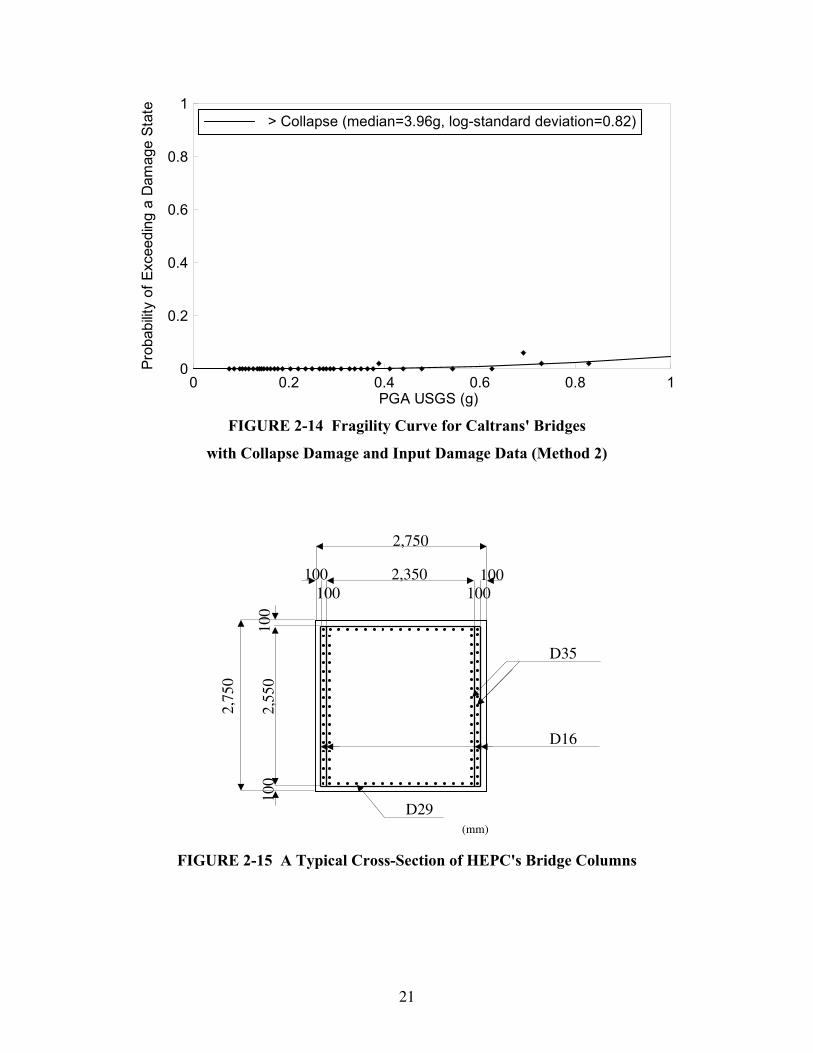
21
0 0.2 0.4 0.6 0.8 1PGA USGS (g)
0
0.2
0.4
0.6
0.8
1
Prob
abilit
y of
Exc
eedi
ng a
Dam
age
Stat
e
> Collapse (median=3.96g, log-standard deviation=0.82)
FIGURE 2-14 Fragility Curve for Caltrans' Bridges
with Collapse Damage and Input Damage Data (Method 2)
FIGURE 2-15 A Typical Cross-Section of HEPC's Bridge Columns
2,750
100100100 100
2,350
100
2,55
0
2,75
0
100
(mm)
D35
D29
D16
22
0 0.2 0.4 0.6 0.8 1PGA (g)
0
0.2
0.4
0.6
0.8
1
Prob
abilit
y of
Exc
eedi
ng a
Dam
age
Stat
e > Minor (median=0.47g, log-standard deviation=0.59) > Moderate (median=0.69g, lod-standard deviation=0.45) > Major (median=0.80g, log-standard deviation=0.43)
KOBE (RC-Single Column)
FIGURE 2-16 Fragility Curves for HEPC's Bridge Columns (Method 1)
0 0.2 0.4 0.6 0.8 1PGA (g)
0
0.2
0.4
0.6
0.8
1
Prob
abilit
y of
Exc
eedi
ng a
Dam
age
Stat
e
> Minor (median=0.47g, log-standard deviation=0.56) > Moderate (median=0.73g, lod-standard deviation=0.56) > Major (median=0.89g, log-standard deviation=0.56)
KOBE (RC-Single Column)
FIGURE 2-17 Fragility Curves for HEPC's Bridge Columns (Method 2)
23
0 0.2 0.4 0.6 0.8 1PGA (g)
0
0.2
0.4
0.6
0.8
1
Prob
abilit
y of
Exc
eedi
ng a
Dam
age
Stat
e
FIGURE 2-18 Fragility Curve for HEPC's Bridge Columns
with at least Minor Damage and Input Damage Data (Method 1)
0 0.2 0.4 0.6 0.8 1PGA (g)
0
0.2
0.4
0.6
0.8
1
Prob
abilit
y of
Exc
eedi
ng a
Dam
age
Stat
e
FIGURE 2-19 Fragility Curve for HEPC's Bridge Columns
with at least Moderate Damage and Input Damage Data (Method 1)
24
0 0.2 0.4 0.6 0.8 1PGA (g)
0
0.2
0.4
0.6
0.8
1
Prob
abilit
y of
Exc
eedi
ng a
Dam
age
Stat
e
FIGURE 2-20 Fragility Curve for HEPC's Bridge Columns
with Major Damage and Input Damage Data (Method 1)
0 0.2 0.4 0.6 0.8 1PGA (g)
0
0.2
0.4
0.6
0.8
1
Prob
abilit
y of
Exc
eedi
ng a
Dam
age
Stat
e
FIGURE 2-21 Fragility Curve for HEPC's Bridge Columns
with at least Minor Damage and Input Damage Data (Method 2)
25
0 0.2 0.4 0.6 0.8 1PGA (g)
0
0.2
0.4
0.6
0.8
1
Prob
abilit
y of
Exc
eedi
ng a
Dam
age
Stat
e
FIGURE 2-22 Fragility Curve for HEPC's Bridge Columns
with at least Moderate Damage and Input Damage Data (Method 2)
0 0.2 0.4 0.6 0.8 1PGA (g)
0
0.2
0.4
0.6
0.8
1
Prob
abilit
y of
Exc
eedi
ng a
Dam
age
Stat
e
FIGURE 2-23 Fragility Curve for HEPC's Bridge Columns
with Major Damage and Input Damage Data (Method 2)
26
TABLE 2-2 Damage Data for Caltrans’ Bridge
(1) (2) (3) (4) (5) (6) (7) (1) (2) (3) (4) (5) (6) (7)
# PGA(g) N ≥ Min ≥ Mod ≥ Maj ≥ Col # PGA(g) N ≥ Min ≥ Mod ≥ Maj ≥ Col 1 0.069 1 0 0 0 0 51 0.078 1 0 0 0 0 2 0.072 1 0 0 0 0 52 0.078 1 0 0 0 0 3 0.072 1 0 0 0 0 53 0.079 1 0 0 0 0 4 0.072 1 0 0 0 0 54 0.079 1 0 0 0 0 5 0.072 1 0 0 0 0 55 0.079 1 0 0 0 0 6 0.072 1 0 0 0 0 56 0.079 1 0 0 0 0 7 0.072 1 0 0 0 0 57 0.079 1 0 0 0 0 8 0.072 1 0 0 0 0 58 0.080 1 0 0 0 0 9 0.073 1 0 0 0 0 59 0.080 1 0 0 0 0 10 0.073 1 0 0 0 0 60 0.080 1 0 0 0 0 11 0.073 1 0 0 0 0 61 0.080 1 0 0 0 0 12 0.074 1 0 0 0 0 62 0.080 1 1 0 0 0 13 0.074 1 0 0 0 0 63 0.080 1 1 0 0 0 14 0.074 1 0 0 0 0 64 0.080 1 0 0 0 0 15 0.074 1 0 0 0 0 65 0.081 1 0 0 0 0 16 0.075 1 0 0 0 0 66 0.081 1 0 0 0 0 17 0.075 1 0 0 0 0 67 0.081 1 0 0 0 0 18 0.075 1 0 0 0 0 68 0.081 1 0 0 0 0 19 0.075 1 0 0 0 0 69 0.082 1 0 0 0 0 20 0.075 1 0 0 0 0 70 0.082 1 0 0 0 0 21 0.075 1 0 0 0 0 71 0.083 1 0 0 0 0 22 0.075 1 0 0 0 0 72 0.083 1 0 0 0 0 23 0.075 1 0 0 0 0 73 0.083 1 0 0 0 0 24 0.075 1 0 0 0 0 74 0.085 1 0 0 0 0 25 0.075 1 0 0 0 0 75 0.085 1 0 0 0 0 26 0.075 1 0 0 0 0 76 0.085 1 0 0 0 0 27 0.075 1 0 0 0 0 77 0.086 1 0 0 0 0 28 0.075 1 0 0 0 0 78 0.087 1 0 0 0 0 29 0.075 1 0 0 0 0 79 0.087 1 0 0 0 0 30 0.075 1 0 0 0 0 80 0.088 1 0 0 0 0 31 0.076 1 0 0 0 0 81 0.090 1 0 0 0 0 32 0.076 1 0 0 0 0 82 0.090 1 0 0 0 0 33 0.076 1 0 0 0 0 83 0.090 1 0 0 0 0 34 0.076 1 0 0 0 0 84 0.090 1 0 0 0 0 35 0.076 1 0 0 0 0 85 0.090 1 0 0 0 0 36 0.076 1 0 0 0 0 86 0.091 1 0 0 0 0 37 0.076 1 0 0 0 0 87 0.091 1 0 0 0 0 38 0.076 1 0 0 0 0 88 0.091 1 0 0 0 0 39 0.076 1 0 0 0 0 89 0.091 1 0 0 0 0 40 0.077 1 0 0 0 0 90 0.091 1 0 0 0 0 41 0.077 1 0 0 0 0 91 0.091 1 0 0 0 0 42 0.077 1 0 0 0 0 92 0.092 1 0 0 0 0 43 0.077 1 0 0 0 0 93 0.092 1 0 0 0 0 44 0.077 1 0 0 0 0 94 0.092 1 0 0 0 0 45 0.077 1 0 0 0 0 95 0.092 1 0 0 0 0 46 0.077 1 0 0 0 0 96 0.092 1 0 0 0 0 47 0.078 1 0 0 0 0 97 0.093 1 0 0 0 0 48 0.078 1 0 0 0 0 98 0.093 1 0 0 0 0 49 0.078 1 0 0 0 0 99 0.093 1 0 0 0 0 50 0.078 1 0 0 0 0 100 0.094 1 0 0 0 0

27
TABLE 2-2 Damage Data for Caltrans’ Bridge (Cont’d)
(1) (2) (3) (4) (5) (6) (7) (1) (2) (3) (4) (5) (6) (7)
# PGA(g) N ≥ Min ≥ Mod ≥ Maj ≥ Col # PGA(g) N ≥ Min ≥ Mod ≥ Maj ≥ Col 101 0.094 1 0 0 0 0 151 0.100 1 0 0 0 0 102 0.094 1 0 0 0 0 152 0.100 1 0 0 0 0 103 0.094 1 0 0 0 0 153 0.100 1 0 0 0 0 104 0.094 1 0 0 0 0 154 0.100 1 0 0 0 0 105 0.095 1 0 0 0 0 155 0.100 1 0 0 0 0 106 0.095 1 0 0 0 0 156 0.100 1 0 0 0 0 107 0.095 1 0 0 0 0 157 0.101 1 0 0 0 0 108 0.095 1 0 0 0 0 158 0.101 1 0 0 0 0 109 0.095 1 0 0 0 0 159 0.101 1 0 0 0 0 110 0.095 1 0 0 0 0 160 0.101 1 0 0 0 0 111 0.096 1 0 0 0 0 161 0.101 1 0 0 0 0 112 0.096 1 0 0 0 0 162 0.102 1 0 0 0 0 113 0.096 1 0 0 0 0 163 0.102 1 0 0 0 0 114 0.096 1 0 0 0 0 164 0.102 1 0 0 0 0 115 0.096 1 0 0 0 0 165 0.102 1 0 0 0 0 116 0.096 1 0 0 0 0 166 0.102 1 0 0 0 0 117 0.096 1 0 0 0 0 167 0.103 1 0 0 0 0 118 0.096 1 0 0 0 0 168 0.103 1 0 0 0 0 119 0.097 1 0 0 0 0 169 0.103 1 0 0 0 0 120 0.097 1 0 0 0 0 170 0.103 1 0 0 0 0 121 0.097 1 0 0 0 0 171 0.103 1 0 0 0 0 122 0.097 1 0 0 0 0 172 0.103 1 0 0 0 0 123 0.097 1 0 0 0 0 173 0.103 1 0 0 0 0 124 0.097 1 0 0 0 0 174 0.103 1 0 0 0 0 125 0.097 1 0 0 0 0 175 0.103 1 0 0 0 0 126 0.097 1 0 0 0 0 176 0.103 1 0 0 0 0 127 0.098 1 0 0 0 0 177 0.103 1 0 0 0 0 128 0.098 1 0 0 0 0 178 0.103 1 0 0 0 0 129 0.098 1 0 0 0 0 179 0.103 1 1 0 0 0 130 0.098 1 0 0 0 0 180 0.103 1 0 0 0 0 131 0.098 1 0 0 0 0 181 0.103 1 0 0 0 0 132 0.098 1 0 0 0 0 182 0.103 1 0 0 0 0 133 0.098 1 0 0 0 0 183 0.103 1 0 0 0 0 134 0.098 1 0 0 0 0 184 0.103 1 0 0 0 0 135 0.098 1 0 0 0 0 185 0.103 1 0 0 0 0 136 0.098 1 0 0 0 0 186 0.103 1 0 0 0 0 137 0.099 1 0 0 0 0 187 0.103 1 0 0 0 0 138 0.099 1 0 0 0 0 188 0.103 1 0 0 0 0 139 0.099 1 0 0 0 0 189 0.103 1 0 0 0 0 140 0.099 1 0 0 0 0 190 0.104 1 1 0 0 0 141 0.099 1 0 0 0 0 191 0.104 1 0 0 0 0 142 0.099 1 0 0 0 0 192 0.104 1 0 0 0 0 143 0.099 1 0 0 0 0 193 0.104 1 0 0 0 0 144 0.099 1 0 0 0 0 194 0.104 1 0 0 0 0 145 0.099 1 0 0 0 0 195 0.104 1 0 0 0 0 146 0.100 1 0 0 0 0 196 0.104 1 0 0 0 0 147 0.100 1 0 0 0 0 197 0.105 1 0 0 0 0 148 0.100 1 0 0 0 0 198 0.105 1 0 0 0 0 149 0.100 1 0 0 0 0 199 0.105 1 0 0 0 0 150 0.100 1 0 0 0 0 200 0.105 1 0 0 0 0
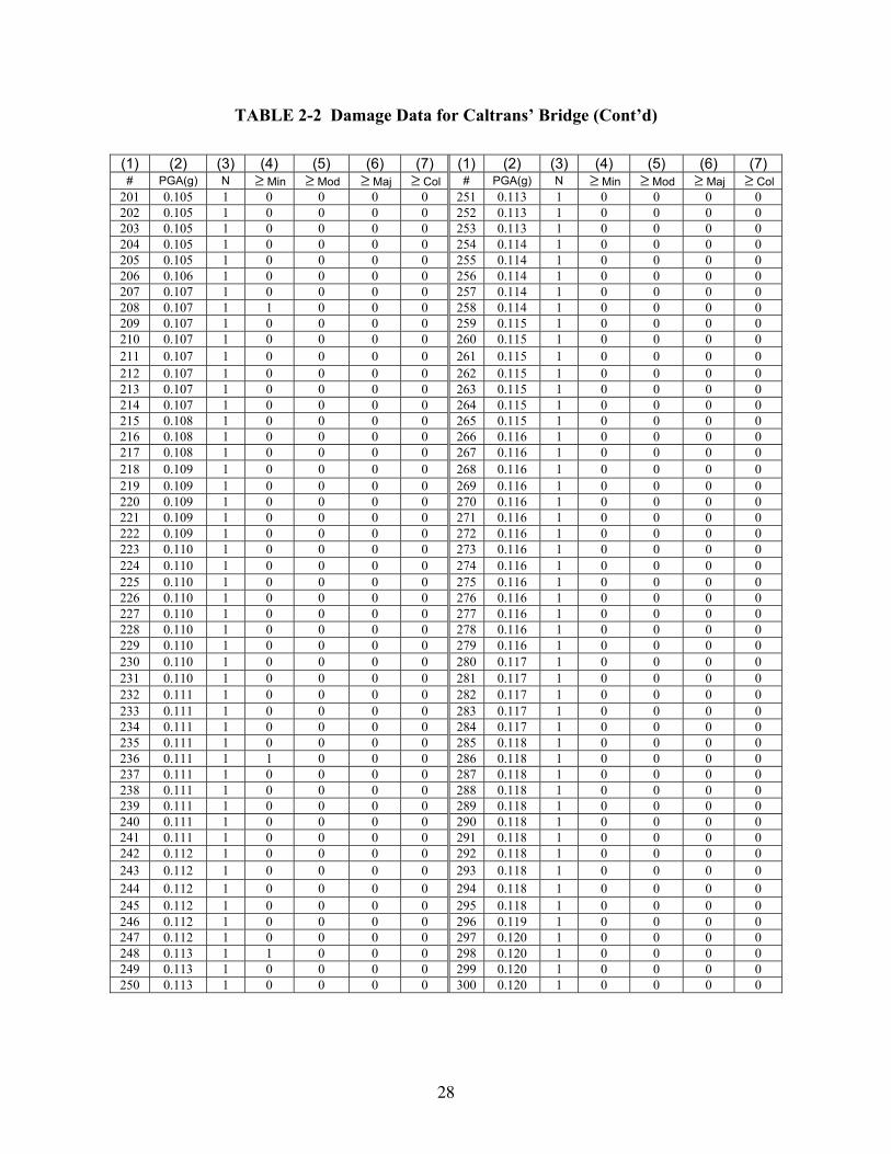
28
TABLE 2-2 Damage Data for Caltrans’ Bridge (Cont’d)
(1) (2) (3) (4) (5) (6) (7) (1) (2) (3) (4) (5) (6) (7) # PGA(g) N ≥ Min ≥ Mod ≥ Maj ≥ Col # PGA(g) N ≥ Min ≥ Mod ≥ Maj ≥ Col
201 0.105 1 0 0 0 0 251 0.113 1 0 0 0 0 202 0.105 1 0 0 0 0 252 0.113 1 0 0 0 0 203 0.105 1 0 0 0 0 253 0.113 1 0 0 0 0 204 0.105 1 0 0 0 0 254 0.114 1 0 0 0 0 205 0.105 1 0 0 0 0 255 0.114 1 0 0 0 0 206 0.106 1 0 0 0 0 256 0.114 1 0 0 0 0 207 0.107 1 0 0 0 0 257 0.114 1 0 0 0 0 208 0.107 1 1 0 0 0 258 0.114 1 0 0 0 0 209 0.107 1 0 0 0 0 259 0.115 1 0 0 0 0 210 0.107 1 0 0 0 0 260 0.115 1 0 0 0 0 211 0.107 1 0 0 0 0 261 0.115 1 0 0 0 0 212 0.107 1 0 0 0 0 262 0.115 1 0 0 0 0 213 0.107 1 0 0 0 0 263 0.115 1 0 0 0 0 214 0.107 1 0 0 0 0 264 0.115 1 0 0 0 0 215 0.108 1 0 0 0 0 265 0.115 1 0 0 0 0 216 0.108 1 0 0 0 0 266 0.116 1 0 0 0 0 217 0.108 1 0 0 0 0 267 0.116 1 0 0 0 0 218 0.109 1 0 0 0 0 268 0.116 1 0 0 0 0 219 0.109 1 0 0 0 0 269 0.116 1 0 0 0 0 220 0.109 1 0 0 0 0 270 0.116 1 0 0 0 0 221 0.109 1 0 0 0 0 271 0.116 1 0 0 0 0 222 0.109 1 0 0 0 0 272 0.116 1 0 0 0 0 223 0.110 1 0 0 0 0 273 0.116 1 0 0 0 0 224 0.110 1 0 0 0 0 274 0.116 1 0 0 0 0 225 0.110 1 0 0 0 0 275 0.116 1 0 0 0 0 226 0.110 1 0 0 0 0 276 0.116 1 0 0 0 0 227 0.110 1 0 0 0 0 277 0.116 1 0 0 0 0 228 0.110 1 0 0 0 0 278 0.116 1 0 0 0 0 229 0.110 1 0 0 0 0 279 0.116 1 0 0 0 0 230 0.110 1 0 0 0 0 280 0.117 1 0 0 0 0 231 0.110 1 0 0 0 0 281 0.117 1 0 0 0 0 232 0.111 1 0 0 0 0 282 0.117 1 0 0 0 0 233 0.111 1 0 0 0 0 283 0.117 1 0 0 0 0 234 0.111 1 0 0 0 0 284 0.117 1 0 0 0 0 235 0.111 1 0 0 0 0 285 0.118 1 0 0 0 0 236 0.111 1 1 0 0 0 286 0.118 1 0 0 0 0 237 0.111 1 0 0 0 0 287 0.118 1 0 0 0 0 238 0.111 1 0 0 0 0 288 0.118 1 0 0 0 0 239 0.111 1 0 0 0 0 289 0.118 1 0 0 0 0 240 0.111 1 0 0 0 0 290 0.118 1 0 0 0 0 241 0.111 1 0 0 0 0 291 0.118 1 0 0 0 0 242 0.112 1 0 0 0 0 292 0.118 1 0 0 0 0 243 0.112 1 0 0 0 0 293 0.118 1 0 0 0 0 244 0.112 1 0 0 0 0 294 0.118 1 0 0 0 0 245 0.112 1 0 0 0 0 295 0.118 1 0 0 0 0 246 0.112 1 0 0 0 0 296 0.119 1 0 0 0 0 247 0.112 1 0 0 0 0 297 0.120 1 0 0 0 0 248 0.113 1 1 0 0 0 298 0.120 1 0 0 0 0 249 0.113 1 0 0 0 0 299 0.120 1 0 0 0 0 250 0.113 1 0 0 0 0 300 0.120 1 0 0 0 0
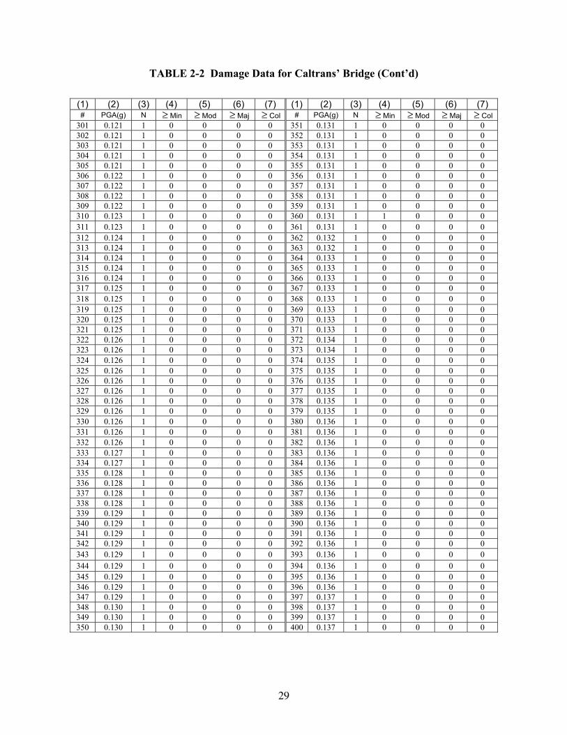
29
TABLE 2-2 Damage Data for Caltrans’ Bridge (Cont’d)
(1) (2) (3) (4) (5) (6) (7) (1) (2) (3) (4) (5) (6) (7) # PGA(g) N ≥ Min ≥ Mod ≥ Maj ≥ Col # PGA(g) N ≥ Min ≥ Mod ≥ Maj ≥ Col
301 0.121 1 0 0 0 0 351 0.131 1 0 0 0 0 302 0.121 1 0 0 0 0 352 0.131 1 0 0 0 0 303 0.121 1 0 0 0 0 353 0.131 1 0 0 0 0 304 0.121 1 0 0 0 0 354 0.131 1 0 0 0 0 305 0.121 1 0 0 0 0 355 0.131 1 0 0 0 0 306 0.122 1 0 0 0 0 356 0.131 1 0 0 0 0 307 0.122 1 0 0 0 0 357 0.131 1 0 0 0 0 308 0.122 1 0 0 0 0 358 0.131 1 0 0 0 0 309 0.122 1 0 0 0 0 359 0.131 1 0 0 0 0 310 0.123 1 0 0 0 0 360 0.131 1 1 0 0 0 311 0.123 1 0 0 0 0 361 0.131 1 0 0 0 0 312 0.124 1 0 0 0 0 362 0.132 1 0 0 0 0 313 0.124 1 0 0 0 0 363 0.132 1 0 0 0 0 314 0.124 1 0 0 0 0 364 0.133 1 0 0 0 0 315 0.124 1 0 0 0 0 365 0.133 1 0 0 0 0 316 0.124 1 0 0 0 0 366 0.133 1 0 0 0 0 317 0.125 1 0 0 0 0 367 0.133 1 0 0 0 0 318 0.125 1 0 0 0 0 368 0.133 1 0 0 0 0 319 0.125 1 0 0 0 0 369 0.133 1 0 0 0 0 320 0.125 1 0 0 0 0 370 0.133 1 0 0 0 0 321 0.125 1 0 0 0 0 371 0.133 1 0 0 0 0 322 0.126 1 0 0 0 0 372 0.134 1 0 0 0 0 323 0.126 1 0 0 0 0 373 0.134 1 0 0 0 0 324 0.126 1 0 0 0 0 374 0.135 1 0 0 0 0 325 0.126 1 0 0 0 0 375 0.135 1 0 0 0 0 326 0.126 1 0 0 0 0 376 0.135 1 0 0 0 0 327 0.126 1 0 0 0 0 377 0.135 1 0 0 0 0 328 0.126 1 0 0 0 0 378 0.135 1 0 0 0 0 329 0.126 1 0 0 0 0 379 0.135 1 0 0 0 0 330 0.126 1 0 0 0 0 380 0.136 1 0 0 0 0 331 0.126 1 0 0 0 0 381 0.136 1 0 0 0 0 332 0.126 1 0 0 0 0 382 0.136 1 0 0 0 0 333 0.127 1 0 0 0 0 383 0.136 1 0 0 0 0 334 0.127 1 0 0 0 0 384 0.136 1 0 0 0 0 335 0.128 1 0 0 0 0 385 0.136 1 0 0 0 0 336 0.128 1 0 0 0 0 386 0.136 1 0 0 0 0 337 0.128 1 0 0 0 0 387 0.136 1 0 0 0 0 338 0.128 1 0 0 0 0 388 0.136 1 0 0 0 0 339 0.129 1 0 0 0 0 389 0.136 1 0 0 0 0 340 0.129 1 0 0 0 0 390 0.136 1 0 0 0 0 341 0.129 1 0 0 0 0 391 0.136 1 0 0 0 0 342 0.129 1 0 0 0 0 392 0.136 1 0 0 0 0 343 0.129 1 0 0 0 0 393 0.136 1 0 0 0 0 344 0.129 1 0 0 0 0 394 0.136 1 0 0 0 0 345 0.129 1 0 0 0 0 395 0.136 1 0 0 0 0 346 0.129 1 0 0 0 0 396 0.136 1 0 0 0 0 347 0.129 1 0 0 0 0 397 0.137 1 0 0 0 0 348 0.130 1 0 0 0 0 398 0.137 1 0 0 0 0 349 0.130 1 0 0 0 0 399 0.137 1 0 0 0 0 350 0.130 1 0 0 0 0 400 0.137 1 0 0 0 0
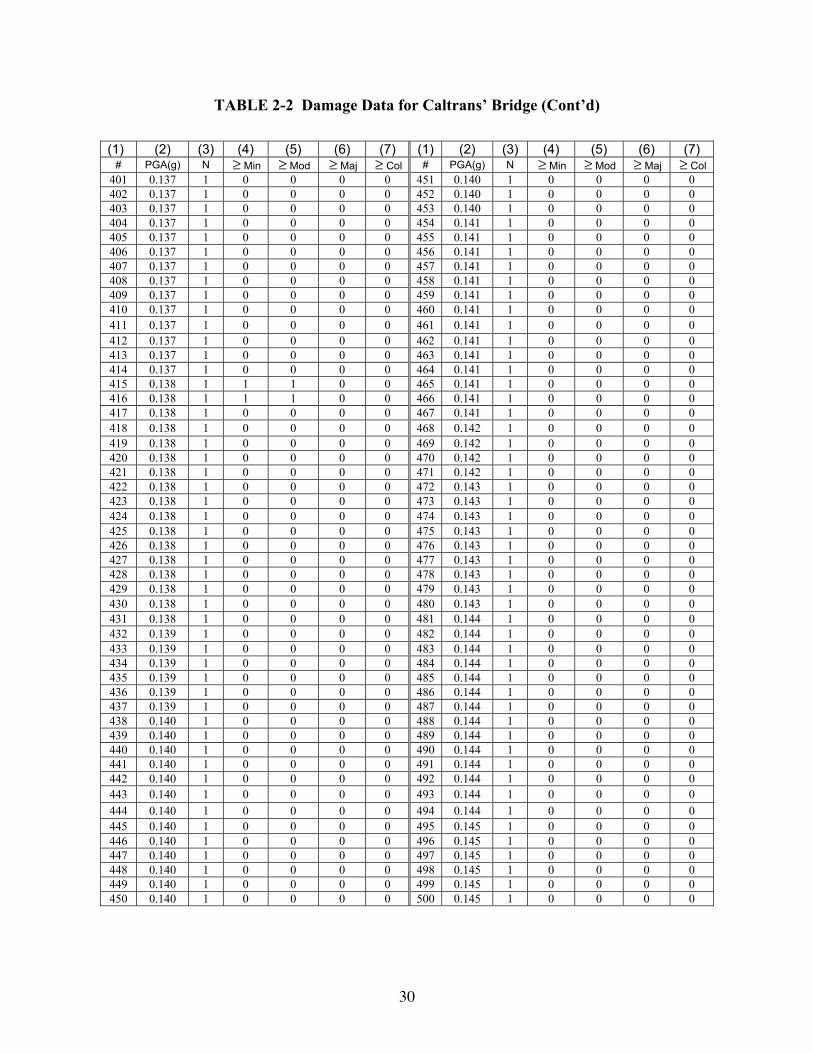
30
TABLE 2-2 Damage Data for Caltrans’ Bridge (Cont’d)
(1) (2) (3) (4) (5) (6) (7) (1) (2) (3) (4) (5) (6) (7)
# PGA(g) N ≥ Min ≥ Mod ≥ Maj ≥ Col # PGA(g) N ≥ Min ≥ Mod ≥ Maj ≥ Col 401 0.137 1 0 0 0 0 451 0.140 1 0 0 0 0 402 0.137 1 0 0 0 0 452 0.140 1 0 0 0 0 403 0.137 1 0 0 0 0 453 0.140 1 0 0 0 0 404 0.137 1 0 0 0 0 454 0.141 1 0 0 0 0 405 0.137 1 0 0 0 0 455 0.141 1 0 0 0 0 406 0.137 1 0 0 0 0 456 0.141 1 0 0 0 0 407 0.137 1 0 0 0 0 457 0.141 1 0 0 0 0 408 0.137 1 0 0 0 0 458 0.141 1 0 0 0 0 409 0.137 1 0 0 0 0 459 0.141 1 0 0 0 0 410 0.137 1 0 0 0 0 460 0.141 1 0 0 0 0 411 0.137 1 0 0 0 0 461 0.141 1 0 0 0 0 412 0.137 1 0 0 0 0 462 0.141 1 0 0 0 0 413 0.137 1 0 0 0 0 463 0.141 1 0 0 0 0 414 0.137 1 0 0 0 0 464 0.141 1 0 0 0 0 415 0.138 1 1 1 0 0 465 0.141 1 0 0 0 0 416 0.138 1 1 1 0 0 466 0.141 1 0 0 0 0 417 0.138 1 0 0 0 0 467 0.141 1 0 0 0 0 418 0.138 1 0 0 0 0 468 0.142 1 0 0 0 0 419 0.138 1 0 0 0 0 469 0.142 1 0 0 0 0 420 0.138 1 0 0 0 0 470 0.142 1 0 0 0 0 421 0.138 1 0 0 0 0 471 0.142 1 0 0 0 0 422 0.138 1 0 0 0 0 472 0.143 1 0 0 0 0 423 0.138 1 0 0 0 0 473 0.143 1 0 0 0 0 424 0.138 1 0 0 0 0 474 0.143 1 0 0 0 0 425 0.138 1 0 0 0 0 475 0.143 1 0 0 0 0 426 0.138 1 0 0 0 0 476 0.143 1 0 0 0 0 427 0.138 1 0 0 0 0 477 0.143 1 0 0 0 0 428 0.138 1 0 0 0 0 478 0.143 1 0 0 0 0 429 0.138 1 0 0 0 0 479 0.143 1 0 0 0 0 430 0.138 1 0 0 0 0 480 0.143 1 0 0 0 0 431 0.138 1 0 0 0 0 481 0.144 1 0 0 0 0 432 0.139 1 0 0 0 0 482 0.144 1 0 0 0 0 433 0.139 1 0 0 0 0 483 0.144 1 0 0 0 0 434 0.139 1 0 0 0 0 484 0.144 1 0 0 0 0 435 0.139 1 0 0 0 0 485 0.144 1 0 0 0 0 436 0.139 1 0 0 0 0 486 0.144 1 0 0 0 0 437 0.139 1 0 0 0 0 487 0.144 1 0 0 0 0 438 0.140 1 0 0 0 0 488 0.144 1 0 0 0 0 439 0.140 1 0 0 0 0 489 0.144 1 0 0 0 0 440 0.140 1 0 0 0 0 490 0.144 1 0 0 0 0 441 0.140 1 0 0 0 0 491 0.144 1 0 0 0 0 442 0.140 1 0 0 0 0 492 0.144 1 0 0 0 0 443 0.140 1 0 0 0 0 493 0.144 1 0 0 0 0 444 0.140 1 0 0 0 0 494 0.144 1 0 0 0 0 445 0.140 1 0 0 0 0 495 0.145 1 0 0 0 0 446 0.140 1 0 0 0 0 496 0.145 1 0 0 0 0 447 0.140 1 0 0 0 0 497 0.145 1 0 0 0 0 448 0.140 1 0 0 0 0 498 0.145 1 0 0 0 0 449 0.140 1 0 0 0 0 499 0.145 1 0 0 0 0 450 0.140 1 0 0 0 0 500 0.145 1 0 0 0 0

31
TABLE 2-2 Damage Data for Caltrans’ Bridge (Cont’d)
(1) (2) (3) (4) (5) (6) (7) (1) (2) (3) (4) (5) (6) (7)
# PGA(g) N ≥ Min ≥ Mod ≥ Maj ≥ Col # PGA(g) N ≥ Min ≥ Mod ≥ Maj ≥ Col 501 0.145 1 0 0 0 0 551 0.151 1 0 0 0 0 502 0.145 1 0 0 0 0 552 0.151 1 0 0 0 0 503 0.145 1 0 0 0 0 553 0.151 1 0 0 0 0 504 0.145 1 0 0 0 0 554 0.151 1 0 0 0 0 505 0.145 1 0 0 0 0 555 0.151 1 0 0 0 0 506 0.145 1 0 0 0 0 556 0.151 1 0 0 0 0 507 0.146 1 0 0 0 0 557 0.152 1 0 0 0 0 508 0.146 1 0 0 0 0 558 0.152 1 0 0 0 0 509 0.146 1 0 0 0 0 559 0.152 1 0 0 0 0 510 0.147 1 0 0 0 0 560 0.153 1 0 0 0 0 511 0.147 1 0 0 0 0 561 0.153 1 0 0 0 0 512 0.147 1 0 0 0 0 562 0.153 1 0 0 0 0 513 0.147 1 0 0 0 0 563 0.153 1 0 0 0 0 514 0.147 1 0 0 0 0 564 0.153 1 1 1 0 0 515 0.147 1 0 0 0 0 565 0.153 1 0 0 0 0 516 0.147 1 0 0 0 0 566 0.153 1 0 0 0 0 517 0.147 1 0 0 0 0 567 0.153 1 0 0 0 0 518 0.147 1 0 0 0 0 568 0.153 1 0 0 0 0 519 0.147 1 0 0 0 0 569 0.153 1 0 0 0 0 520 0.147 1 0 0 0 0 570 0.153 1 0 0 0 0 521 0.147 1 0 0 0 0 571 0.153 1 0 0 0 0 522 0.147 1 0 0 0 0 572 0.154 1 0 0 0 0 523 0.147 1 0 0 0 0 573 0.154 1 0 0 0 0 524 0.147 1 0 0 0 0 574 0.154 1 0 0 0 0 525 0.148 1 0 0 0 0 575 0.154 1 0 0 0 0 526 0.148 1 0 0 0 0 576 0.154 1 0 0 0 0 527 0.148 1 0 0 0 0 577 0.154 1 0 0 0 0 528 0.148 1 0 0 0 0 578 0.155 1 0 0 0 0 529 0.148 1 0 0 0 0 579 0.155 1 0 0 0 0 530 0.148 1 0 0 0 0 580 0.155 1 0 0 0 0 531 0.148 1 0 0 0 0 581 0.155 1 0 0 0 0 532 0.149 1 0 0 0 0 582 0.156 1 0 0 0 0 533 0.149 1 0 0 0 0 583 0.156 1 0 0 0 0 534 0.149 1 0 0 0 0 584 0.157 1 0 0 0 0 535 0.149 1 0 0 0 0 585 0.157 1 0 0 0 0 536 0.149 1 0 0 0 0 586 0.157 1 0 0 0 0 537 0.149 1 0 0 0 0 587 0.157 1 0 0 0 0 538 0.149 1 0 0 0 0 588 0.157 1 0 0 0 0 539 0.149 1 0 0 0 0 589 0.157 1 1 0 0 0 540 0.149 1 0 0 0 0 590 0.157 1 0 0 0 0 541 0.150 1 0 0 0 0 591 0.157 1 0 0 0 0 542 0.150 1 0 0 0 0 592 0.157 1 0 0 0 0 543 0.150 1 0 0 0 0 593 0.158 1 0 0 0 0 544 0.150 1 0 0 0 0 594 0.158 1 0 0 0 0 545 0.150 1 0 0 0 0 595 0.158 1 0 0 0 0 546 0.150 1 0 0 0 0 596 0.158 1 0 0 0 0 547 0.150 1 0 0 0 0 597 0.158 1 0 0 0 0 548 0.150 1 0 0 0 0 598 0.158 1 0 0 0 0 549 0.150 1 0 0 0 0 599 0.158 1 0 0 0 0 550 0.150 1 0 0 0 0 600 0.158 1 0 0 0 0
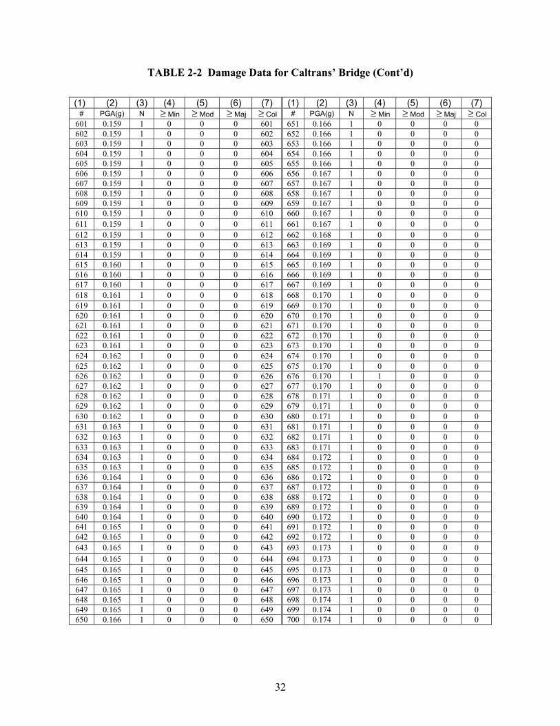
32
TABLE 2-2 Damage Data for Caltrans’ Bridge (Cont’d)
(1) (2) (3) (4) (5) (6) (7) (1) (2) (3) (4) (5) (6) (7)
# PGA(g) N ≥ Min ≥ Mod ≥ Maj ≥ Col # PGA(g) N ≥ Min ≥ Mod ≥ Maj ≥ Col 601 0.159 1 0 0 0 601 651 0.166 1 0 0 0 0 602 0.159 1 0 0 0 602 652 0.166 1 0 0 0 0 603 0.159 1 0 0 0 603 653 0.166 1 0 0 0 0 604 0.159 1 0 0 0 604 654 0.166 1 0 0 0 0 605 0.159 1 0 0 0 605 655 0.166 1 0 0 0 0 606 0.159 1 0 0 0 606 656 0.167 1 0 0 0 0 607 0.159 1 0 0 0 607 657 0.167 1 0 0 0 0 608 0.159 1 0 0 0 608 658 0.167 1 0 0 0 0 609 0.159 1 0 0 0 609 659 0.167 1 0 0 0 0 610 0.159 1 0 0 0 610 660 0.167 1 0 0 0 0 611 0.159 1 0 0 0 611 661 0.167 1 0 0 0 0 612 0.159 1 0 0 0 612 662 0.168 1 0 0 0 0 613 0.159 1 0 0 0 613 663 0.169 1 0 0 0 0 614 0.159 1 0 0 0 614 664 0.169 1 0 0 0 0 615 0.160 1 0 0 0 615 665 0.169 1 0 0 0 0 616 0.160 1 0 0 0 616 666 0.169 1 0 0 0 0 617 0.160 1 0 0 0 617 667 0.169 1 0 0 0 0 618 0.161 1 0 0 0 618 668 0.170 1 0 0 0 0 619 0.161 1 0 0 0 619 669 0.170 1 0 0 0 0 620 0.161 1 0 0 0 620 670 0.170 1 0 0 0 0 621 0.161 1 0 0 0 621 671 0.170 1 0 0 0 0 622 0.161 1 0 0 0 622 672 0.170 1 0 0 0 0 623 0.161 1 0 0 0 623 673 0.170 1 0 0 0 0 624 0.162 1 0 0 0 624 674 0.170 1 0 0 0 0 625 0.162 1 0 0 0 625 675 0.170 1 0 0 0 0 626 0.162 1 0 0 0 626 676 0.170 1 1 0 0 0 627 0.162 1 0 0 0 627 677 0.170 1 0 0 0 0 628 0.162 1 0 0 0 628 678 0.171 1 0 0 0 0 629 0.162 1 0 0 0 629 679 0.171 1 0 0 0 0 630 0.162 1 0 0 0 630 680 0.171 1 0 0 0 0 631 0.163 1 0 0 0 631 681 0.171 1 0 0 0 0 632 0.163 1 0 0 0 632 682 0.171 1 0 0 0 0 633 0.163 1 0 0 0 633 683 0.171 1 0 0 0 0 634 0.163 1 0 0 0 634 684 0.172 1 0 0 0 0 635 0.163 1 0 0 0 635 685 0.172 1 0 0 0 0 636 0.164 1 0 0 0 636 686 0.172 1 0 0 0 0 637 0.164 1 0 0 0 637 687 0.172 1 0 0 0 0 638 0.164 1 0 0 0 638 688 0.172 1 0 0 0 0 639 0.164 1 0 0 0 639 689 0.172 1 0 0 0 0 640 0.164 1 0 0 0 640 690 0.172 1 0 0 0 0 641 0.165 1 0 0 0 641 691 0.172 1 0 0 0 0 642 0.165 1 0 0 0 642 692 0.172 1 0 0 0 0 643 0.165 1 0 0 0 643 693 0.173 1 0 0 0 0 644 0.165 1 0 0 0 644 694 0.173 1 0 0 0 0 645 0.165 1 0 0 0 645 695 0.173 1 0 0 0 0 646 0.165 1 0 0 0 646 696 0.173 1 0 0 0 0 647 0.165 1 0 0 0 647 697 0.173 1 0 0 0 0 648 0.165 1 0 0 0 648 698 0.174 1 0 0 0 0 649 0.165 1 0 0 0 649 699 0.174 1 0 0 0 0 650 0.166 1 0 0 0 650 700 0.174 1 0 0 0 0

33
TABLE 2-2 Damage Data for Caltrans’ Bridge (Cont’d)
(1) (2) (3) (4) (5) (6) (7) (1) (2) (3) (4) (5) (6) (7)
# PGA(g) N ≥ Min ≥ Mod ≥ Maj ≥ Col # PGA(g) N ≥ Min ≥ Mod ≥ Maj ≥ Col 701 0.174 1 0 0 0 0 751 0.182 1 0 0 0 0 702 0.174 1 0 0 0 0 752 0.182 1 0 0 0 0 703 0.174 1 0 0 0 0 753 0.183 1 0 0 0 0 704 0.175 1 0 0 0 0 754 0.183 1 0 0 0 0 705 0.175 1 0 0 0 0 755 0.183 1 0 0 0 0 706 0.175 1 0 0 0 0 756 0.183 1 0 0 0 0 707 0.175 1 0 0 0 0 757 0.183 1 0 0 0 0 708 0.175 1 0 0 0 0 758 0.183 1 0 0 0 0 709 0.175 1 0 0 0 0 759 0.183 1 0 0 0 0 710 0.175 1 0 0 0 0 760 0.183 1 0 0 0 0 711 0.175 1 0 0 0 0 761 0.183 1 0 0 0 0 712 0.175 1 0 0 0 0 762 0.184 1 0 0 0 0 713 0.176 1 0 0 0 0 763 0.184 1 0 0 0 0 714 0.176 1 0 0 0 0 764 0.184 1 0 0 0 0 715 0.176 1 0 0 0 0 765 0.184 1 0 0 0 0 716 0.176 1 0 0 0 0 766 0.184 1 0 0 0 0 717 0.177 1 0 0 0 0 767 0.184 1 0 0 0 0 718 0.177 1 0 0 0 0 768 0.184 1 0 0 0 0 719 0.177 1 0 0 0 0 769 0.184 1 0 0 0 0 720 0.177 1 0 0 0 0 770 0.184 1 0 0 0 0 721 0.177 1 0 0 0 0 771 0.184 1 0 0 0 0 722 0.177 1 0 0 0 0 772 0.184 1 0 0 0 0 723 0.177 1 0 0 0 0 773 0.184 1 0 0 0 0 724 0.177 1 0 0 0 0 774 0.184 1 0 0 0 0 725 0.177 1 0 0 0 0 775 0.185 1 0 0 0 0 726 0.178 1 0 0 0 0 776 0.185 1 0 0 0 0 727 0.178 1 0 0 0 0 777 0.185 1 0 0 0 0 728 0.178 1 0 0 0 0 778 0.185 1 0 0 0 0 729 0.178 1 0 0 0 0 779 0.186 1 0 0 0 0 730 0.178 1 0 0 0 0 780 0.186 1 0 0 0 0 731 0.178 1 0 0 0 0 781 0.188 1 0 0 0 0 732 0.178 1 0 0 0 0 782 0.188 1 0 0 0 0 733 0.178 1 0 0 0 0 783 0.188 1 0 0 0 0 734 0.178 1 0 0 0 0 784 0.189 1 0 0 0 0 735 0.179 1 0 0 0 0 785 0.189 1 0 0 0 0 736 0.179 1 0 0 0 0 786 0.189 1 0 0 0 0 737 0.179 1 0 0 0 0 787 0.190 1 0 0 0 0 738 0.179 1 0 0 0 0 788 0.191 1 0 0 0 0 739 0.179 1 0 0 0 0 789 0.191 1 0 0 0 0 740 0.179 1 0 0 0 0 790 0.193 1 0 0 0 0 741 0.179 1 0 0 0 0 791 0.193 1 0 0 0 0 742 0.179 1 0 0 0 0 792 0.194 1 0 0 0 0 743 0.179 1 0 0 0 0 793 0.194 1 0 0 0 0 744 0.179 1 0 0 0 0 794 0.194 1 0 0 0 0 745 0.179 1 0 0 0 0 795 0.194 1 0 0 0 0 746 0.179 1 0 0 0 0 796 0.195 1 0 0 0 0 747 0.179 1 0 0 0 0 797 0.195 1 0 0 0 0 748 0.181 1 0 0 0 0 798 0.195 1 0 0 0 0 749 0.181 1 0 0 0 0 799 0.196 1 0 0 0 0 750 0.181 1 0 0 0 0 800 0.196 1 0 0 0 0

34
TABLE 2-2 Damage Data for Caltrans’ Bridge (Cont’d)
(1) (2) (3) (4) (5) (6) (7) (1) (2) (3) (4) (5) (6) (7) # PGA(g) N ≥ Min ≥ Mod ≥ Maj ≥ Col # PGA(g) N ≥ Min ≥ Mod ≥ Maj ≥ Col
801 0.196 1 0 0 0 0 851 0.211 1 0 0 0 0 802 0.196 1 0 0 0 0 852 0.212 1 0 0 0 0 803 0.196 1 0 0 0 0 853 0.213 1 0 0 0 0 804 0.196 1 0 0 0 0 854 0.213 1 1 1 0 0 805 0.196 1 0 0 0 0 855 0.213 1 0 0 0 0 806 0.197 1 0 0 0 0 856 0.213 1 0 0 0 0 807 0.197 1 0 0 0 0 857 0.213 1 0 0 0 0 808 0.198 1 0 0 0 0 858 0.214 1 0 0 0 0 809 0.198 1 0 0 0 0 859 0.215 1 0 0 0 0 810 0.200 1 0 0 0 0 860 0.217 1 0 0 0 0 811 0.200 1 0 0 0 0 861 0.217 1 0 0 0 0 812 0.200 1 0 0 0 0 862 0.217 1 0 0 0 0 813 0.200 1 0 0 0 0 863 0.217 1 0 0 0 0 814 0.200 1 0 0 0 0 864 0.217 1 0 0 0 0 815 0.201 1 0 0 0 0 865 0.217 1 0 0 0 0 816 0.202 1 0 0 0 0 866 0.217 1 0 0 0 0 817 0.202 1 0 0 0 0 867 0.217 1 0 0 0 0 818 0.202 1 0 0 0 0 868 0.217 1 0 0 0 0 819 0.203 1 0 0 0 0 869 0.217 1 0 0 0 0 820 0.203 1 0 0 0 0 870 0.217 1 0 0 0 0 821 0.203 1 0 0 0 0 871 0.217 1 0 0 0 0 822 0.203 1 0 0 0 0 872 0.217 1 0 0 0 0 823 0.203 1 0 0 0 0 873 0.217 1 0 0 0 0 824 0.204 1 0 0 0 0 874 0.221 1 0 0 0 0 825 0.205 1 0 0 0 0 875 0.221 1 0 0 0 0 826 0.206 1 0 0 0 0 876 0.221 1 0 0 0 0 827 0.206 1 0 0 0 0 877 0.221 1 0 0 0 0 828 0.206 1 0 0 0 0 878 0.221 1 0 0 0 0 829 0.206 1 0 0 0 0 879 0.221 1 0 0 0 0 830 0.207 1 0 0 0 0 880 0.222 1 0 0 0 0 831 0.207 1 0 0 0 0 881 0.222 1 0 0 0 0 832 0.207 1 0 0 0 0 882 0.222 1 0 0 0 0 833 0.207 1 0 0 0 0 883 0.222 1 0 0 0 0 834 0.207 1 0 0 0 0 884 0.223 1 0 0 0 0 835 0.207 1 0 0 0 0 885 0.223 1 0 0 0 0 836 0.207 1 0 0 0 0 886 0.226 1 0 0 0 0 837 0.207 1 0 0 0 0 887 0.226 1 0 0 0 0 838 0.207 1 0 0 0 0 888 0.226 1 0 0 0 0 839 0.207 1 0 0 0 0 889 0.226 1 0 0 0 0 840 0.207 1 0 0 0 0 890 0.226 1 0 0 0 0 841 0.207 1 0 0 0 0 891 0.226 1 0 0 0 0 842 0.209 1 0 0 0 0 892 0.226 1 0 0 0 0 843 0.209 1 0 0 0 0 893 0.226 1 0 0 0 0 844 0.209 1 0 0 0 0 894 0.226 1 0 0 0 0 845 0.210 1 0 0 0 0 895 0.226 1 0 0 0 0 846 0.210 1 0 0 0 0 896 0.227 1 0 0 0 0 847 0.210 1 0 0 0 0 897 0.227 1 0 0 0 0 848 0.210 1 0 0 0 0 898 0.227 1 0 0 0 0 849 0.210 1 0 0 0 0 899 0.227 1 0 0 0 0 850 0.211 1 0 0 0 0 900 0.227 1 1 0 0 0
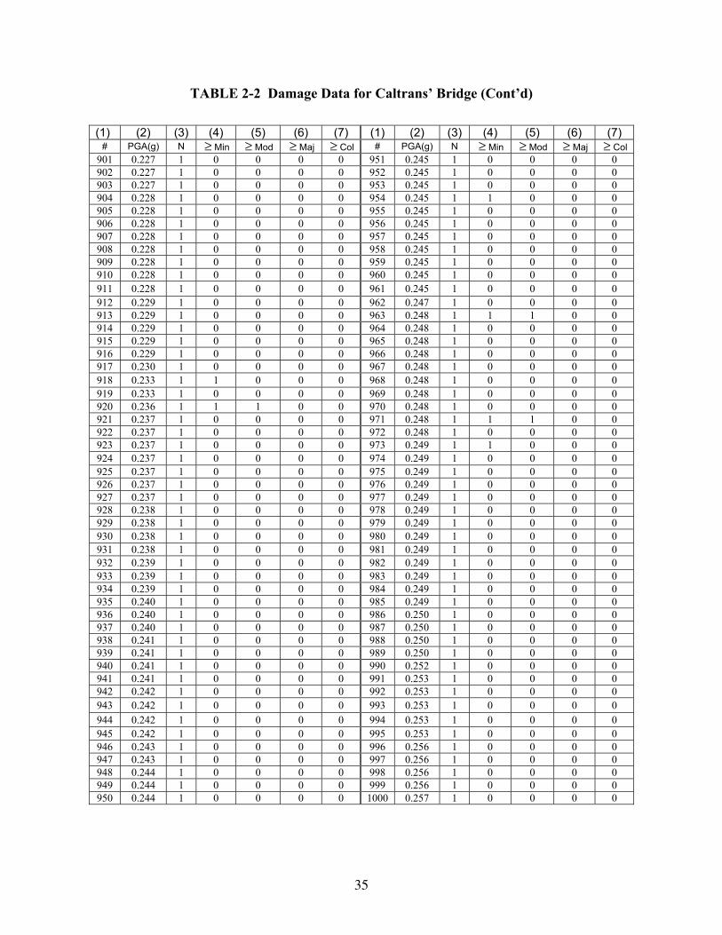
35
TABLE 2-2 Damage Data for Caltrans’ Bridge (Cont’d)
(1) (2) (3) (4) (5) (6) (7) (1) (2) (3) (4) (5) (6) (7)
# PGA(g) N ≥ Min ≥ Mod ≥ Maj ≥ Col # PGA(g) N ≥ Min ≥ Mod ≥ Maj ≥ Col 901 0.227 1 0 0 0 0 951 0.245 1 0 0 0 0 902 0.227 1 0 0 0 0 952 0.245 1 0 0 0 0 903 0.227 1 0 0 0 0 953 0.245 1 0 0 0 0 904 0.228 1 0 0 0 0 954 0.245 1 1 0 0 0 905 0.228 1 0 0 0 0 955 0.245 1 0 0 0 0 906 0.228 1 0 0 0 0 956 0.245 1 0 0 0 0 907 0.228 1 0 0 0 0 957 0.245 1 0 0 0 0 908 0.228 1 0 0 0 0 958 0.245 1 0 0 0 0 909 0.228 1 0 0 0 0 959 0.245 1 0 0 0 0 910 0.228 1 0 0 0 0 960 0.245 1 0 0 0 0 911 0.228 1 0 0 0 0 961 0.245 1 0 0 0 0 912 0.229 1 0 0 0 0 962 0.247 1 0 0 0 0 913 0.229 1 0 0 0 0 963 0.248 1 1 1 0 0 914 0.229 1 0 0 0 0 964 0.248 1 0 0 0 0 915 0.229 1 0 0 0 0 965 0.248 1 0 0 0 0 916 0.229 1 0 0 0 0 966 0.248 1 0 0 0 0 917 0.230 1 0 0 0 0 967 0.248 1 0 0 0 0 918 0.233 1 1 0 0 0 968 0.248 1 0 0 0 0 919 0.233 1 0 0 0 0 969 0.248 1 0 0 0 0 920 0.236 1 1 1 0 0 970 0.248 1 0 0 0 0 921 0.237 1 0 0 0 0 971 0.248 1 1 1 0 0 922 0.237 1 0 0 0 0 972 0.248 1 0 0 0 0 923 0.237 1 0 0 0 0 973 0.249 1 1 0 0 0 924 0.237 1 0 0 0 0 974 0.249 1 0 0 0 0 925 0.237 1 0 0 0 0 975 0.249 1 0 0 0 0 926 0.237 1 0 0 0 0 976 0.249 1 0 0 0 0 927 0.237 1 0 0 0 0 977 0.249 1 0 0 0 0 928 0.238 1 0 0 0 0 978 0.249 1 0 0 0 0 929 0.238 1 0 0 0 0 979 0.249 1 0 0 0 0 930 0.238 1 0 0 0 0 980 0.249 1 0 0 0 0 931 0.238 1 0 0 0 0 981 0.249 1 0 0 0 0 932 0.239 1 0 0 0 0 982 0.249 1 0 0 0 0 933 0.239 1 0 0 0 0 983 0.249 1 0 0 0 0 934 0.239 1 0 0 0 0 984 0.249 1 0 0 0 0 935 0.240 1 0 0 0 0 985 0.249 1 0 0 0 0 936 0.240 1 0 0 0 0 986 0.250 1 0 0 0 0 937 0.240 1 0 0 0 0 987 0.250 1 0 0 0 0 938 0.241 1 0 0 0 0 988 0.250 1 0 0 0 0 939 0.241 1 0 0 0 0 989 0.250 1 0 0 0 0 940 0.241 1 0 0 0 0 990 0.252 1 0 0 0 0 941 0.241 1 0 0 0 0 991 0.253 1 0 0 0 0 942 0.242 1 0 0 0 0 992 0.253 1 0 0 0 0 943 0.242 1 0 0 0 0 993 0.253 1 0 0 0 0 944 0.242 1 0 0 0 0 994 0.253 1 0 0 0 0 945 0.242 1 0 0 0 0 995 0.253 1 0 0 0 0 946 0.243 1 0 0 0 0 996 0.256 1 0 0 0 0 947 0.243 1 0 0 0 0 997 0.256 1 0 0 0 0 948 0.244 1 0 0 0 0 998 0.256 1 0 0 0 0 949 0.244 1 0 0 0 0 999 0.256 1 0 0 0 0 950 0.244 1 0 0 0 0 1000 0.257 1 0 0 0 0
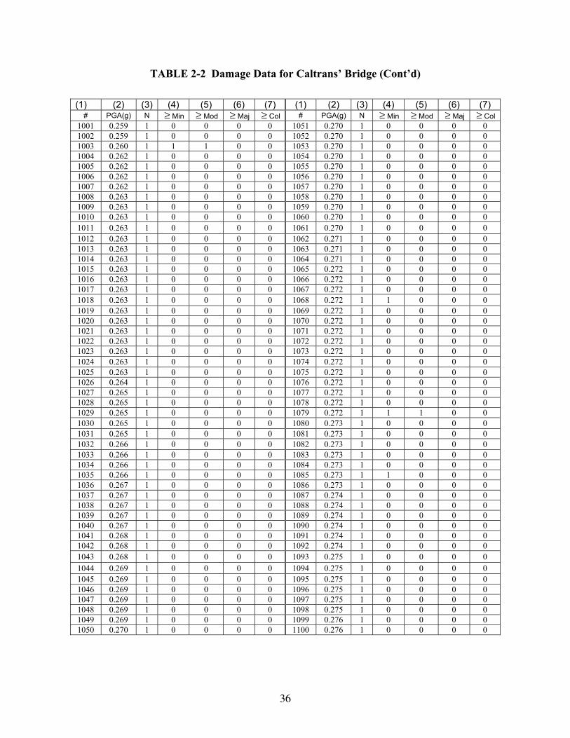
36
TABLE 2-2 Damage Data for Caltrans’ Bridge (Cont’d)
(1) (2) (3) (4) (5) (6) (7) (1) (2) (3) (4) (5) (6) (7)
# PGA(g) N ≥ Min ≥ Mod ≥ Maj ≥ Col # PGA(g) N ≥ Min ≥ Mod ≥ Maj ≥ Col 1001 0.259 1 0 0 0 0 1051 0.270 1 0 0 0 0 1002 0.259 1 0 0 0 0 1052 0.270 1 0 0 0 0 1003 0.260 1 1 1 0 0 1053 0.270 1 0 0 0 0 1004 0.262 1 0 0 0 0 1054 0.270 1 0 0 0 0 1005 0.262 1 0 0 0 0 1055 0.270 1 0 0 0 0 1006 0.262 1 0 0 0 0 1056 0.270 1 0 0 0 0 1007 0.262 1 0 0 0 0 1057 0.270 1 0 0 0 0 1008 0.263 1 0 0 0 0 1058 0.270 1 0 0 0 0 1009 0.263 1 0 0 0 0 1059 0.270 1 0 0 0 0 1010 0.263 1 0 0 0 0 1060 0.270 1 0 0 0 0 1011 0.263 1 0 0 0 0 1061 0.270 1 0 0 0 0 1012 0.263 1 0 0 0 0 1062 0.271 1 0 0 0 0 1013 0.263 1 0 0 0 0 1063 0.271 1 0 0 0 0 1014 0.263 1 0 0 0 0 1064 0.271 1 0 0 0 0 1015 0.263 1 0 0 0 0 1065 0.272 1 0 0 0 0 1016 0.263 1 0 0 0 0 1066 0.272 1 0 0 0 0 1017 0.263 1 0 0 0 0 1067 0.272 1 0 0 0 0 1018 0.263 1 0 0 0 0 1068 0.272 1 1 0 0 0 1019 0.263 1 0 0 0 0 1069 0.272 1 0 0 0 0 1020 0.263 1 0 0 0 0 1070 0.272 1 0 0 0 0 1021 0.263 1 0 0 0 0 1071 0.272 1 0 0 0 0 1022 0.263 1 0 0 0 0 1072 0.272 1 0 0 0 0 1023 0.263 1 0 0 0 0 1073 0.272 1 0 0 0 0 1024 0.263 1 0 0 0 0 1074 0.272 1 0 0 0 0 1025 0.263 1 0 0 0 0 1075 0.272 1 0 0 0 0 1026 0.264 1 0 0 0 0 1076 0.272 1 0 0 0 0 1027 0.265 1 0 0 0 0 1077 0.272 1 0 0 0 0 1028 0.265 1 0 0 0 0 1078 0.272 1 0 0 0 0 1029 0.265 1 0 0 0 0 1079 0.272 1 1 1 0 0 1030 0.265 1 0 0 0 0 1080 0.273 1 0 0 0 0 1031 0.265 1 0 0 0 0 1081 0.273 1 0 0 0 0 1032 0.266 1 0 0 0 0 1082 0.273 1 0 0 0 0 1033 0.266 1 0 0 0 0 1083 0.273 1 0 0 0 0 1034 0.266 1 0 0 0 0 1084 0.273 1 0 0 0 0 1035 0.266 1 0 0 0 0 1085 0.273 1 1 0 0 0 1036 0.267 1 0 0 0 0 1086 0.273 1 0 0 0 0 1037 0.267 1 0 0 0 0 1087 0.274 1 0 0 0 0 1038 0.267 1 0 0 0 0 1088 0.274 1 0 0 0 0 1039 0.267 1 0 0 0 0 1089 0.274 1 0 0 0 0 1040 0.267 1 0 0 0 0 1090 0.274 1 0 0 0 0 1041 0.268 1 0 0 0 0 1091 0.274 1 0 0 0 0 1042 0.268 1 0 0 0 0 1092 0.274 1 0 0 0 0 1043 0.268 1 0 0 0 0 1093 0.275 1 0 0 0 0 1044 0.269 1 0 0 0 0 1094 0.275 1 0 0 0 0 1045 0.269 1 0 0 0 0 1095 0.275 1 0 0 0 0 1046 0.269 1 0 0 0 0 1096 0.275 1 0 0 0 0 1047 0.269 1 0 0 0 0 1097 0.275 1 0 0 0 0 1048 0.269 1 0 0 0 0 1098 0.275 1 0 0 0 0 1049 0.269 1 0 0 0 0 1099 0.276 1 0 0 0 0 1050 0.270 1 0 0 0 0 1100 0.276 1 0 0 0 0
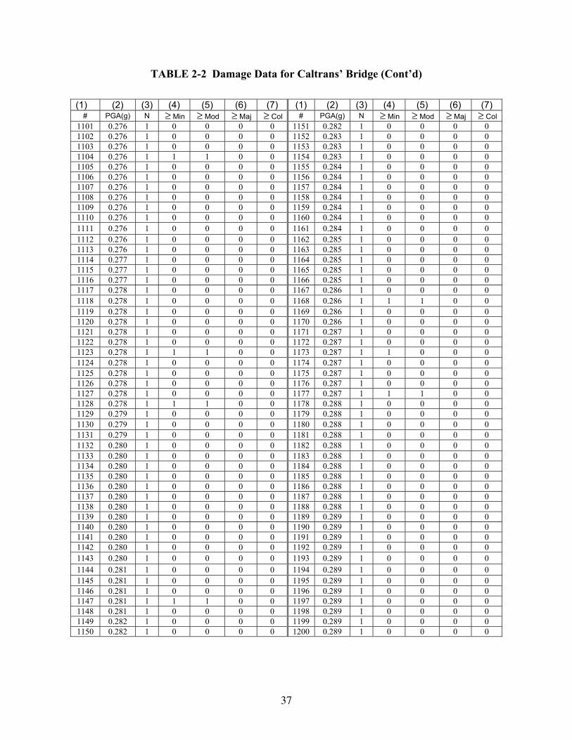
37
TABLE 2-2 Damage Data for Caltrans’ Bridge (Cont’d)
(1) (2) (3) (4) (5) (6) (7) (1) (2) (3) (4) (5) (6) (7)
# PGA(g) N ≥ Min ≥ Mod ≥ Maj ≥ Col # PGA(g) N ≥ Min ≥ Mod ≥ Maj ≥ Col 1101 0.276 1 0 0 0 0 1151 0.282 1 0 0 0 0 1102 0.276 1 0 0 0 0 1152 0.283 1 0 0 0 0 1103 0.276 1 0 0 0 0 1153 0.283 1 0 0 0 0 1104 0.276 1 1 1 0 0 1154 0.283 1 0 0 0 0 1105 0.276 1 0 0 0 0 1155 0.284 1 0 0 0 0 1106 0.276 1 0 0 0 0 1156 0.284 1 0 0 0 0 1107 0.276 1 0 0 0 0 1157 0.284 1 0 0 0 0 1108 0.276 1 0 0 0 0 1158 0.284 1 0 0 0 0 1109 0.276 1 0 0 0 0 1159 0.284 1 0 0 0 0 1110 0.276 1 0 0 0 0 1160 0.284 1 0 0 0 0 1111 0.276 1 0 0 0 0 1161 0.284 1 0 0 0 0 1112 0.276 1 0 0 0 0 1162 0.285 1 0 0 0 0 1113 0.276 1 0 0 0 0 1163 0.285 1 0 0 0 0 1114 0.277 1 0 0 0 0 1164 0.285 1 0 0 0 0 1115 0.277 1 0 0 0 0 1165 0.285 1 0 0 0 0 1116 0.277 1 0 0 0 0 1166 0.285 1 0 0 0 0 1117 0.278 1 0 0 0 0 1167 0.286 1 0 0 0 0 1118 0.278 1 0 0 0 0 1168 0.286 1 1 1 0 0 1119 0.278 1 0 0 0 0 1169 0.286 1 0 0 0 0 1120 0.278 1 0 0 0 0 1170 0.286 1 0 0 0 0 1121 0.278 1 0 0 0 0 1171 0.287 1 0 0 0 0 1122 0.278 1 0 0 0 0 1172 0.287 1 0 0 0 0 1123 0.278 1 1 1 0 0 1173 0.287 1 1 0 0 0 1124 0.278 1 0 0 0 0 1174 0.287 1 0 0 0 0 1125 0.278 1 0 0 0 0 1175 0.287 1 0 0 0 0 1126 0.278 1 0 0 0 0 1176 0.287 1 0 0 0 0 1127 0.278 1 0 0 0 0 1177 0.287 1 1 1 0 0 1128 0.278 1 1 1 0 0 1178 0.288 1 0 0 0 0 1129 0.279 1 0 0 0 0 1179 0.288 1 0 0 0 0 1130 0.279 1 0 0 0 0 1180 0.288 1 0 0 0 0 1131 0.279 1 0 0 0 0 1181 0.288 1 0 0 0 0 1132 0.280 1 0 0 0 0 1182 0.288 1 0 0 0 0 1133 0.280 1 0 0 0 0 1183 0.288 1 0 0 0 0 1134 0.280 1 0 0 0 0 1184 0.288 1 0 0 0 0 1135 0.280 1 0 0 0 0 1185 0.288 1 0 0 0 0 1136 0.280 1 0 0 0 0 1186 0.288 1 0 0 0 0 1137 0.280 1 0 0 0 0 1187 0.288 1 0 0 0 0 1138 0.280 1 0 0 0 0 1188 0.288 1 0 0 0 0 1139 0.280 1 0 0 0 0 1189 0.289 1 0 0 0 0 1140 0.280 1 0 0 0 0 1190 0.289 1 0 0 0 0 1141 0.280 1 0 0 0 0 1191 0.289 1 0 0 0 0 1142 0.280 1 0 0 0 0 1192 0.289 1 0 0 0 0 1143 0.280 1 0 0 0 0 1193 0.289 1 0 0 0 0 1144 0.281 1 0 0 0 0 1194 0.289 1 0 0 0 0 1145 0.281 1 0 0 0 0 1195 0.289 1 0 0 0 0 1146 0.281 1 0 0 0 0 1196 0.289 1 0 0 0 0 1147 0.281 1 1 1 0 0 1197 0.289 1 0 0 0 0 1148 0.281 1 0 0 0 0 1198 0.289 1 0 0 0 0 1149 0.282 1 0 0 0 0 1199 0.289 1 0 0 0 0 1150 0.282 1 0 0 0 0 1200 0.289 1 0 0 0 0
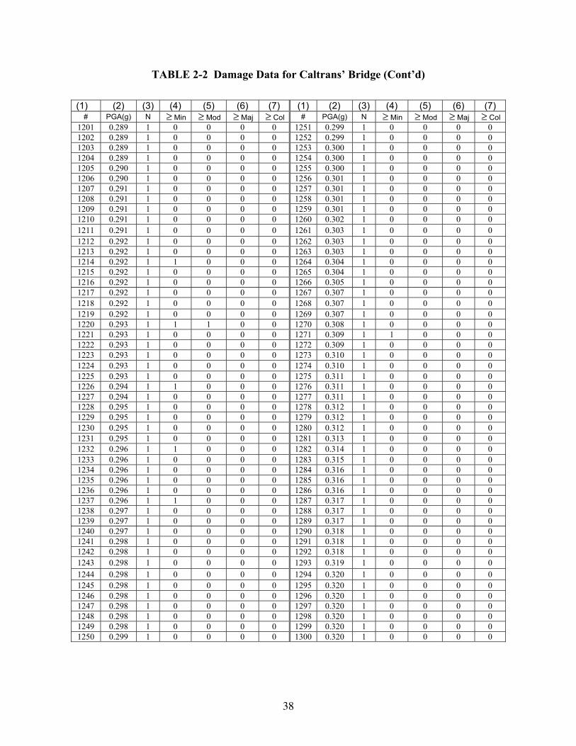
38
TABLE 2-2 Damage Data for Caltrans’ Bridge (Cont’d)
(1) (2) (3) (4) (5) (6) (7) (1) (2) (3) (4) (5) (6) (7)
# PGA(g) N ≥ Min ≥ Mod ≥ Maj ≥ Col # PGA(g) N ≥ Min ≥ Mod ≥ Maj ≥ Col 1201 0.289 1 0 0 0 0 1251 0.299 1 0 0 0 0 1202 0.289 1 0 0 0 0 1252 0.299 1 0 0 0 0 1203 0.289 1 0 0 0 0 1253 0.300 1 0 0 0 0 1204 0.289 1 0 0 0 0 1254 0.300 1 0 0 0 0 1205 0.290 1 0 0 0 0 1255 0.300 1 0 0 0 0 1206 0.290 1 0 0 0 0 1256 0.301 1 0 0 0 0 1207 0.291 1 0 0 0 0 1257 0.301 1 0 0 0 0 1208 0.291 1 0 0 0 0 1258 0.301 1 0 0 0 0 1209 0.291 1 0 0 0 0 1259 0.301 1 0 0 0 0 1210 0.291 1 0 0 0 0 1260 0.302 1 0 0 0 0 1211 0.291 1 0 0 0 0 1261 0.303 1 0 0 0 0 1212 0.292 1 0 0 0 0 1262 0.303 1 0 0 0 0 1213 0.292 1 0 0 0 0 1263 0.303 1 0 0 0 0 1214 0.292 1 1 0 0 0 1264 0.304 1 0 0 0 0 1215 0.292 1 0 0 0 0 1265 0.304 1 0 0 0 0 1216 0.292 1 0 0 0 0 1266 0.305 1 0 0 0 0 1217 0.292 1 0 0 0 0 1267 0.307 1 0 0 0 0 1218 0.292 1 0 0 0 0 1268 0.307 1 0 0 0 0 1219 0.292 1 0 0 0 0 1269 0.307 1 0 0 0 0 1220 0.293 1 1 1 0 0 1270 0.308 1 0 0 0 0 1221 0.293 1 0 0 0 0 1271 0.309 1 1 0 0 0 1222 0.293 1 0 0 0 0 1272 0.309 1 0 0 0 0 1223 0.293 1 0 0 0 0 1273 0.310 1 0 0 0 0 1224 0.293 1 0 0 0 0 1274 0.310 1 0 0 0 0 1225 0.293 1 0 0 0 0 1275 0.311 1 0 0 0 0 1226 0.294 1 1 0 0 0 1276 0.311 1 0 0 0 0 1227 0.294 1 0 0 0 0 1277 0.311 1 0 0 0 0 1228 0.295 1 0 0 0 0 1278 0.312 1 0 0 0 0 1229 0.295 1 0 0 0 0 1279 0.312 1 0 0 0 0 1230 0.295 1 0 0 0 0 1280 0.312 1 0 0 0 0 1231 0.295 1 0 0 0 0 1281 0.313 1 0 0 0 0 1232 0.296 1 1 0 0 0 1282 0.314 1 0 0 0 0 1233 0.296 1 0 0 0 0 1283 0.315 1 0 0 0 0 1234 0.296 1 0 0 0 0 1284 0.316 1 0 0 0 0 1235 0.296 1 0 0 0 0 1285 0.316 1 0 0 0 0 1236 0.296 1 0 0 0 0 1286 0.316 1 0 0 0 0 1237 0.296 1 1 0 0 0 1287 0.317 1 0 0 0 0 1238 0.297 1 0 0 0 0 1288 0.317 1 0 0 0 0 1239 0.297 1 0 0 0 0 1289 0.317 1 0 0 0 0 1240 0.297 1 0 0 0 0 1290 0.318 1 0 0 0 0 1241 0.298 1 0 0 0 0 1291 0.318 1 0 0 0 0 1242 0.298 1 0 0 0 0 1292 0.318 1 0 0 0 0 1243 0.298 1 0 0 0 0 1293 0.319 1 0 0 0 0 1244 0.298 1 0 0 0 0 1294 0.320 1 0 0 0 0 1245 0.298 1 0 0 0 0 1295 0.320 1 0 0 0 0 1246 0.298 1 0 0 0 0 1296 0.320 1 0 0 0 0 1247 0.298 1 0 0 0 0 1297 0.320 1 0 0 0 0 1248 0.298 1 0 0 0 0 1298 0.320 1 0 0 0 0 1249 0.298 1 0 0 0 0 1299 0.320 1 0 0 0 0 1250 0.299 1 0 0 0 0 1300 0.320 1 0 0 0 0
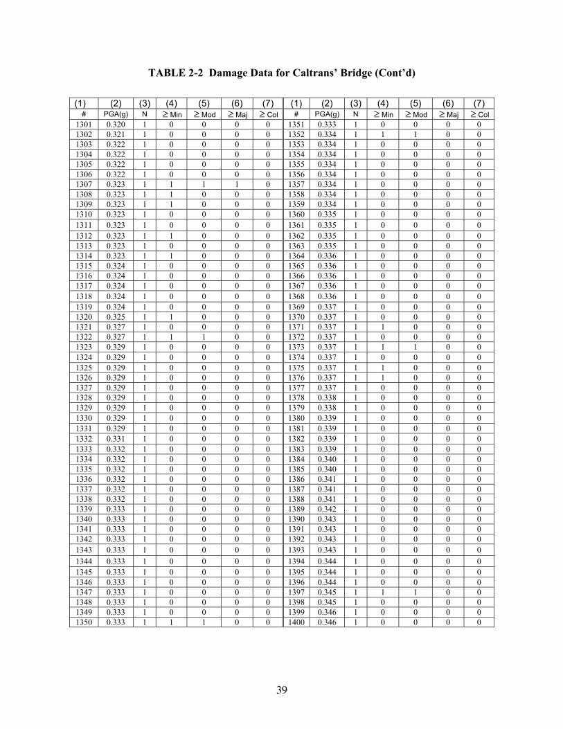
39
TABLE 2-2 Damage Data for Caltrans’ Bridge (Cont’d)
(1) (2) (3) (4) (5) (6) (7) (1) (2) (3) (4) (5) (6) (7)
# PGA(g) N ≥ Min ≥ Mod ≥ Maj ≥ Col # PGA(g) N ≥ Min ≥ Mod ≥ Maj ≥ Col 1301 0.320 1 0 0 0 0 1351 0.333 1 0 0 0 0 1302 0.321 1 0 0 0 0 1352 0.334 1 1 1 0 0 1303 0.322 1 0 0 0 0 1353 0.334 1 0 0 0 0 1304 0.322 1 0 0 0 0 1354 0.334 1 0 0 0 0 1305 0.322 1 0 0 0 0 1355 0.334 1 0 0 0 0 1306 0.322 1 0 0 0 0 1356 0.334 1 0 0 0 0 1307 0.323 1 1 1 1 0 1357 0.334 1 0 0 0 0 1308 0.323 1 1 0 0 0 1358 0.334 1 0 0 0 0 1309 0.323 1 1 0 0 0 1359 0.334 1 0 0 0 0 1310 0.323 1 0 0 0 0 1360 0.335 1 0 0 0 0 1311 0.323 1 0 0 0 0 1361 0.335 1 0 0 0 0 1312 0.323 1 1 0 0 0 1362 0.335 1 0 0 0 0 1313 0.323 1 0 0 0 0 1363 0.335 1 0 0 0 0 1314 0.323 1 1 0 0 0 1364 0.336 1 0 0 0 0 1315 0.324 1 0 0 0 0 1365 0.336 1 0 0 0 0 1316 0.324 1 0 0 0 0 1366 0.336 1 0 0 0 0 1317 0.324 1 0 0 0 0 1367 0.336 1 0 0 0 0 1318 0.324 1 0 0 0 0 1368 0.336 1 0 0 0 0 1319 0.324 1 0 0 0 0 1369 0.337 1 0 0 0 0 1320 0.325 1 1 0 0 0 1370 0.337 1 0 0 0 0 1321 0.327 1 0 0 0 0 1371 0.337 1 1 0 0 0 1322 0.327 1 1 1 0 0 1372 0.337 1 0 0 0 0 1323 0.329 1 0 0 0 0 1373 0.337 1 1 1 0 0 1324 0.329 1 0 0 0 0 1374 0.337 1 0 0 0 0 1325 0.329 1 0 0 0 0 1375 0.337 1 1 0 0 0 1326 0.329 1 0 0 0 0 1376 0.337 1 1 0 0 0 1327 0.329 1 0 0 0 0 1377 0.337 1 0 0 0 0 1328 0.329 1 0 0 0 0 1378 0.338 1 0 0 0 0 1329 0.329 1 0 0 0 0 1379 0.338 1 0 0 0 0 1330 0.329 1 0 0 0 0 1380 0.339 1 0 0 0 0 1331 0.329 1 0 0 0 0 1381 0.339 1 0 0 0 0 1332 0.331 1 0 0 0 0 1382 0.339 1 0 0 0 0 1333 0.332 1 0 0 0 0 1383 0.339 1 0 0 0 0 1334 0.332 1 0 0 0 0 1384 0.340 1 0 0 0 0 1335 0.332 1 0 0 0 0 1385 0.340 1 0 0 0 0 1336 0.332 1 0 0 0 0 1386 0.341 1 0 0 0 0 1337 0.332 1 0 0 0 0 1387 0.341 1 0 0 0 0 1338 0.332 1 0 0 0 0 1388 0.341 1 0 0 0 0 1339 0.333 1 0 0 0 0 1389 0.342 1 0 0 0 0 1340 0.333 1 0 0 0 0 1390 0.343 1 0 0 0 0 1341 0.333 1 0 0 0 0 1391 0.343 1 0 0 0 0 1342 0.333 1 0 0 0 0 1392 0.343 1 0 0 0 0 1343 0.333 1 0 0 0 0 1393 0.343 1 0 0 0 0 1344 0.333 1 0 0 0 0 1394 0.344 1 0 0 0 0 1345 0.333 1 0 0 0 0 1395 0.344 1 0 0 0 0 1346 0.333 1 0 0 0 0 1396 0.344 1 0 0 0 0 1347 0.333 1 0 0 0 0 1397 0.345 1 1 1 0 0 1348 0.333 1 0 0 0 0 1398 0.345 1 0 0 0 0 1349 0.333 1 0 0 0 0 1399 0.346 1 0 0 0 0 1350 0.333 1 1 1 0 0 1400 0.346 1 0 0 0 0
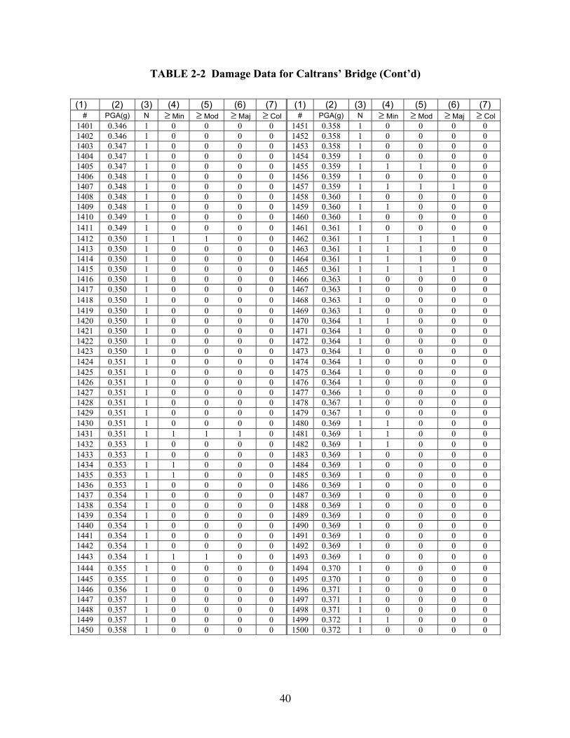
40
TABLE 2-2 Damage Data for Caltrans’ Bridge (Cont’d)
(1) (2) (3) (4) (5) (6) (7) (1) (2) (3) (4) (5) (6) (7)
# PGA(g) N ≥ Min ≥ Mod ≥ Maj ≥ Col # PGA(g) N ≥ Min ≥ Mod ≥ Maj ≥ Col 1401 0.346 1 0 0 0 0 1451 0.358 1 0 0 0 0 1402 0.346 1 0 0 0 0 1452 0.358 1 0 0 0 0 1403 0.347 1 0 0 0 0 1453 0.358 1 0 0 0 0 1404 0.347 1 0 0 0 0 1454 0.359 1 0 0 0 0 1405 0.347 1 0 0 0 0 1455 0.359 1 1 1 0 0 1406 0.348 1 0 0 0 0 1456 0.359 1 0 0 0 0 1407 0.348 1 0 0 0 0 1457 0.359 1 1 1 1 0 1408 0.348 1 0 0 0 0 1458 0.360 1 0 0 0 0 1409 0.348 1 0 0 0 0 1459 0.360 1 1 0 0 0 1410 0.349 1 0 0 0 0 1460 0.360 1 0 0 0 0 1411 0.349 1 0 0 0 0 1461 0.361 1 0 0 0 0 1412 0.350 1 1 1 0 0 1462 0.361 1 1 1 1 0 1413 0.350 1 0 0 0 0 1463 0.361 1 1 1 0 0 1414 0.350 1 0 0 0 0 1464 0.361 1 1 1 0 0 1415 0.350 1 0 0 0 0 1465 0.361 1 1 1 1 0 1416 0.350 1 0 0 0 0 1466 0.363 1 0 0 0 0 1417 0.350 1 0 0 0 0 1467 0.363 1 0 0 0 0 1418 0.350 1 0 0 0 0 1468 0.363 1 0 0 0 0 1419 0.350 1 0 0 0 0 1469 0.363 1 0 0 0 0 1420 0.350 1 0 0 0 0 1470 0.364 1 1 0 0 0 1421 0.350 1 0 0 0 0 1471 0.364 1 0 0 0 0 1422 0.350 1 0 0 0 0 1472 0.364 1 0 0 0 0 1423 0.350 1 0 0 0 0 1473 0.364 1 0 0 0 0 1424 0.351 1 0 0 0 0 1474 0.364 1 0 0 0 0 1425 0.351 1 0 0 0 0 1475 0.364 1 0 0 0 0 1426 0.351 1 0 0 0 0 1476 0.364 1 0 0 0 0 1427 0.351 1 0 0 0 0 1477 0.366 1 0 0 0 0 1428 0.351 1 0 0 0 0 1478 0.367 1 0 0 0 0 1429 0.351 1 0 0 0 0 1479 0.367 1 0 0 0 0 1430 0.351 1 0 0 0 0 1480 0.369 1 1 0 0 0 1431 0.351 1 1 1 1 0 1481 0.369 1 1 0 0 0 1432 0.353 1 0 0 0 0 1482 0.369 1 1 0 0 0 1433 0.353 1 0 0 0 0 1483 0.369 1 0 0 0 0 1434 0.353 1 1 0 0 0 1484 0.369 1 0 0 0 0 1435 0.353 1 1 0 0 0 1485 0.369 1 0 0 0 0 1436 0.353 1 0 0 0 0 1486 0.369 1 0 0 0 0 1437 0.354 1 0 0 0 0 1487 0.369 1 0 0 0 0 1438 0.354 1 0 0 0 0 1488 0.369 1 0 0 0 0 1439 0.354 1 0 0 0 0 1489 0.369 1 0 0 0 0 1440 0.354 1 0 0 0 0 1490 0.369 1 0 0 0 0 1441 0.354 1 0 0 0 0 1491 0.369 1 0 0 0 0 1442 0.354 1 0 0 0 0 1492 0.369 1 0 0 0 0 1443 0.354 1 1 1 0 0 1493 0.369 1 0 0 0 0 1444 0.355 1 0 0 0 0 1494 0.370 1 0 0 0 0 1445 0.355 1 0 0 0 0 1495 0.370 1 0 0 0 0 1446 0.356 1 0 0 0 0 1496 0.371 1 0 0 0 0 1447 0.357 1 0 0 0 0 1497 0.371 1 0 0 0 0 1448 0.357 1 0 0 0 0 1498 0.371 1 0 0 0 0 1449 0.357 1 0 0 0 0 1499 0.372 1 1 0 0 0 1450 0.358 1 0 0 0 0 1500 0.372 1 0 0 0 0

41
TABLE 2-2 Damage Data for Caltrans’ Bridge (Cont’d)
(1) (2) (3) (4) (5) (6) (7) (1) (2) (3) (4) (5) (6) (7)
# PGA(g) N ≥ Min ≥ Mod ≥ Maj ≥ Col # PGA(g) N ≥ Min ≥ Mod ≥ Maj ≥ Col 1501 0.372 1 0 0 0 0 1551 0.383 1 0 0 0 0 1502 0.372 1 0 0 0 0 1552 0.383 1 0 0 0 0 1503 0.372 1 0 0 0 0 1553 0.383 1 1 1 0 0 1504 0.372 1 0 0 0 0 1554 0.383 1 1 0 0 0 1505 0.372 1 0 0 0 0 1555 0.384 1 0 0 0 0 1506 0.372 1 1 0 0 0 1556 0.385 1 1 0 0 0 1507 0.373 1 0 0 0 0 1557 0.385 1 0 0 0 0 1508 0.373 1 0 0 0 0 1558 0.385 1 1 0 0 0 1509 0.373 1 0 0 0 0 1559 0.385 1 0 0 0 0 1510 0.373 1 0 0 0 0 1560 0.385 1 0 0 0 0 1511 0.373 1 0 0 0 0 1561 0.385 1 1 1 1 1 1512 0.373 1 0 0 0 0 1562 0.385 1 1 1 1 0 1513 0.373 1 1 1 1 0 1563 0.385 1 0 0 0 0 1514 0.373 1 1 1 0 0 1564 0.385 1 0 0 0 0 1515 0.374 1 0 0 0 0 1565 0.386 1 1 0 0 0 1516 0.375 1 0 0 0 0 1566 0.386 1 0 0 0 0 1517 0.375 1 1 0 0 0 1567 0.387 1 0 0 0 0 1518 0.375 1 1 1 0 0 1568 0.387 1 0 0 0 0 1519 0.376 1 0 0 0 0 1569 0.387 1 0 0 0 0 1520 0.376 1 0 0 0 0 1570 0.387 1 0 0 0 0 1521 0.376 1 0 0 0 0 1571 0.388 1 1 1 0 0 1522 0.377 1 1 0 0 0 1572 0.388 1 0 0 0 0 1523 0.377 1 0 0 0 0 1573 0.389 1 0 0 0 0 1524 0.377 1 0 0 0 0 1574 0.390 1 1 0 0 0 1525 0.377 1 0 0 0 0 1575 0.390 1 0 0 0 0 1526 0.377 1 0 0 0 0 1576 0.390 1 0 0 0 0 1527 0.377 1 0 0 0 0 1577 0.390 1 0 0 0 0 1528 0.377 1 0 0 0 0 1578 0.390 1 0 0 0 0 1529 0.378 1 0 0 0 0 1579 0.390 1 0 0 0 0 1530 0.378 1 0 0 0 0 1580 0.390 1 0 0 0 0 1531 0.378 1 0 0 0 0 1581 0.390 1 1 1 0 0 1532 0.380 1 0 0 0 0 1582 0.390 1 1 1 0 0 1533 0.380 1 1 0 0 0 1583 0.390 1 0 0 0 0 1534 0.380 1 1 1 0 0 1584 0.390 1 1 0 0 0 1535 0.380 1 1 0 0 0 1585 0.390 1 1 1 0 0 1536 0.380 1 0 0 0 0 1586 0.390 1 1 1 1 0 1537 0.380 1 0 0 0 0 1587 0.391 1 0 0 0 0 1538 0.380 1 1 0 0 0 1588 0.391 1 0 0 0 0 1539 0.380 1 0 0 0 0 1589 0.392 1 1 0 0 0 1540 0.380 1 1 0 0 0 1590 0.393 1 0 0 0 0 1541 0.380 1 0 0 0 0 1591 0.393 1 1 0 0 0 1542 0.380 1 0 0 0 0 1592 0.393 1 1 0 0 0 1543 0.380 1 0 0 0 0 1593 0.394 1 0 0 0 0 1544 0.381 1 0 0 0 0 1594 0.394 1 1 1 0 0 1545 0.381 1 0 0 0 0 1595 0.395 1 0 0 0 0 1546 0.381 1 0 0 0 0 1596 0.395 1 0 0 0 0 1547 0.381 1 0 0 0 0 1597 0.395 1 0 0 0 0 1548 0.381 1 0 0 0 0 1598 0.395 1 0 0 0 0 1549 0.382 1 0 0 0 0 1599 0.395 1 0 0 0 0 1550 0.383 1 0 0 0 0 1600 0.395 1 0 0 0 0
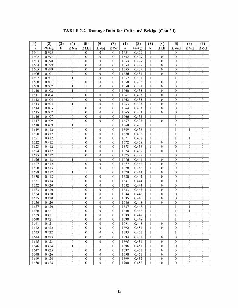
42
TABLE 2-2 Damage Data for Caltrans’ Bridge (Cont’d)
(1) (2) (3) (4) (5) (6) (7) (1) (2) (3) (4) (5) (6) (7)
# PGA(g) N ≥ Min ≥ Mod ≥ Maj ≥ Col # PGA(g) N ≥ Min ≥ Mod ≥ Maj ≥ Col 1601 0.395 1 0 0 0 0 1651 0.429 1 1 0 0 0 1602 0.397 1 0 0 0 0 1652 0.429 1 0 0 0 0 1603 0.398 1 0 0 0 0 1653 0.429 1 0 0 0 0 1604 0.398 1 0 0 0 0 1654 0.429 1 0 0 0 0 1605 0.399 1 0 0 0 0 1655 0.429 1 0 0 0 0 1606 0.401 1 0 0 0 0 1656 0.431 1 0 0 0 0 1607 0.401 1 1 1 0 0 1657 0.431 1 1 1 0 0 1608 0.401 1 0 0 0 0 1658 0.432 1 0 0 0 0 1609 0.402 1 1 1 0 0 1659 0.432 1 0 0 0 0 1610 0.402 1 1 1 1 0 1660 0.433 1 0 0 0 0 1611 0.404 1 0 0 0 0 1661 0.433 1 0 0 0 0 1612 0.404 1 0 0 0 0 1662 0.433 1 0 0 0 0 1613 0.404 1 1 1 0 0 1663 0.433 1 0 0 0 0 1614 0.405 1 0 0 0 0 1664 0.433 1 0 0 0 0 1615 0.407 1 0 0 0 0 1665 0.434 1 0 0 0 0 1616 0.407 1 0 0 0 0 1666 0.434 1 1 1 0 0 1617 0.409 1 0 0 0 0 1667 0.435 1 0 0 0 0 1618 0.409 1 1 1 1 0 1668 0.436 1 1 1 0 0 1619 0.412 1 0 0 0 0 1669 0.436 1 1 1 1 0 1620 0.412 1 0 0 0 0 1670 0.436 1 1 1 0 0 1621 0.412 1 0 0 0 0 1671 0.438 1 1 1 1 0 1622 0.412 1 0 0 0 0 1672 0.438 1 0 0 0 0 1623 0.412 1 0 0 0 0 1673 0.438 1 0 0 0 0 1624 0.412 1 0 0 0 0 1674 0.439 1 0 0 0 0 1625 0.412 1 0 0 0 0 1675 0.439 1 1 0 0 0 1626 0.412 1 1 1 0 0 1676 0.441 1 0 0 0 0 1627 0.412 1 0 0 0 0 1677 0.442 1 0 0 0 0 1628 0.413 1 0 0 0 0 1678 0.442 1 0 0 0 0 1629 0.417 1 1 1 1 0 1679 0.444 1 0 0 0 0 1630 0.418 1 0 0 0 0 1680 0.444 1 0 0 0 0 1631 0.418 1 0 0 0 0 1681 0.444 1 0 0 0 0 1632 0.420 1 0 0 0 0 1682 0.444 1 0 0 0 0 1633 0.420 1 0 0 0 0 1683 0.445 1 0 0 0 0 1634 0.420 1 0 0 0 0 1684 0.445 1 0 0 0 0 1635 0.420 1 0 0 0 0 1685 0.446 1 0 0 0 0 1636 0.420 1 0 0 0 0 1686 0.448 1 0 0 0 0 1637 0.420 1 0 0 0 0 1687 0.448 1 1 1 1 0 1638 0.421 1 0 0 0 0 1688 0.448 1 1 1 1 0 1639 0.421 1 0 0 0 0 1689 0.448 1 1 1 0 0 1640 0.421 1 0 0 0 0 1690 0.448 1 1 1 0 0 1641 0.421 1 0 0 0 0 1691 0.448 1 0 0 0 0 1642 0.422 1 0 0 0 0 1692 0.451 1 0 0 0 0 1643 0.422 1 0 0 0 0 1693 0.451 1 1 1 0 0 1644 0.423 1 0 0 0 0 1694 0.451 1 0 0 0 0 1645 0.423 1 0 0 0 0 1695 0.451 1 0 0 0 0 1646 0.424 1 1 1 1 0 1696 0.451 1 0 0 0 0 1647 0.425 1 0 0 0 0 1697 0.451 1 0 0 0 0 1648 0.426 1 0 0 0 0 1698 0.451 1 0 0 0 0 1649 0.426 1 0 0 0 0 1699 0.452 1 0 0 0 0 1650 0.428 1 0 0 0 0 1700 0.452 1 0 0 0 0
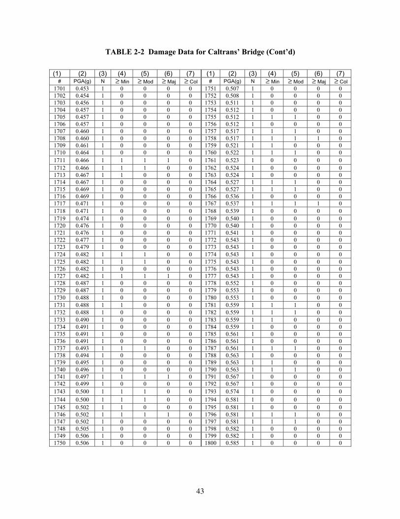
43
TABLE 2-2 Damage Data for Caltrans’ Bridge (Cont’d)
(1) (2) (3) (4) (5) (6) (7) (1) (2) (3) (4) (5) (6) (7)
# PGA(g) N ≥ Min ≥ Mod ≥ Maj ≥ Col # PGA(g) N ≥ Min ≥ Mod ≥ Maj ≥ Col 1701 0.453 1 0 0 0 0 1751 0.507 1 0 0 0 0 1702 0.454 1 0 0 0 0 1752 0.508 1 0 0 0 0 1703 0.456 1 0 0 0 0 1753 0.511 1 0 0 0 0 1704 0.457 1 0 0 0 0 1754 0.512 1 0 0 0 0 1705 0.457 1 0 0 0 0 1755 0.512 1 1 1 0 0 1706 0.457 1 0 0 0 0 1756 0.512 1 0 0 0 0 1707 0.460 1 0 0 0 0 1757 0.517 1 1 1 0 0 1708 0.460 1 0 0 0 0 1758 0.517 1 1 1 1 0 1709 0.461 1 0 0 0 0 1759 0.521 1 1 0 0 0 1710 0.464 1 0 0 0 0 1760 0.522 1 1 1 0 0 1711 0.466 1 1 1 1 0 1761 0.523 1 0 0 0 0 1712 0.466 1 1 1 0 0 1762 0.524 1 0 0 0 0 1713 0.467 1 1 0 0 0 1763 0.524 1 0 0 0 0 1714 0.467 1 0 0 0 0 1764 0.527 1 1 1 0 0 1715 0.469 1 0 0 0 0 1765 0.527 1 1 1 0 0 1716 0.469 1 0 0 0 0 1766 0.536 1 0 0 0 0 1717 0.471 1 0 0 0 0 1767 0.537 1 1 1 1 0 1718 0.471 1 0 0 0 0 1768 0.539 1 0 0 0 0 1719 0.474 1 0 0 0 0 1769 0.540 1 0 0 0 0 1720 0.476 1 0 0 0 0 1770 0.540 1 0 0 0 0 1721 0.476 1 0 0 0 0 1771 0.541 1 0 0 0 0 1722 0.477 1 0 0 0 0 1772 0.543 1 0 0 0 0 1723 0.479 1 0 0 0 0 1773 0.543 1 0 0 0 0 1724 0.482 1 1 1 0 0 1774 0.543 1 0 0 0 0 1725 0.482 1 1 1 0 0 1775 0.543 1 0 0 0 0 1726 0.482 1 0 0 0 0 1776 0.543 1 0 0 0 0 1727 0.482 1 1 1 1 0 1777 0.543 1 0 0 0 0 1728 0.487 1 0 0 0 0 1778 0.552 1 0 0 0 0 1729 0.487 1 0 0 0 0 1779 0.553 1 0 0 0 0 1730 0.488 1 0 0 0 0 1780 0.553 1 0 0 0 0 1731 0.488 1 1 0 0 0 1781 0.559 1 1 1 0 0 1732 0.488 1 0 0 0 0 1782 0.559 1 1 1 0 0 1733 0.490 1 0 0 0 0 1783 0.559 1 1 0 0 0 1734 0.491 1 0 0 0 0 1784 0.559 1 0 0 0 0 1735 0.491 1 0 0 0 0 1785 0.561 1 0 0 0 0 1736 0.491 1 0 0 0 0 1786 0.561 1 0 0 0 0 1737 0.493 1 1 1 0 0 1787 0.561 1 1 1 0 0 1738 0.494 1 0 0 0 0 1788 0.563 1 0 0 0 0 1739 0.495 1 0 0 0 0 1789 0.563 1 1 0 0 0 1740 0.496 1 0 0 0 0 1790 0.563 1 1 1 0 0 1741 0.497 1 1 1 1 0 1791 0.567 1 0 0 0 0 1742 0.499 1 0 0 0 0 1792 0.567 1 0 0 0 0 1743 0.500 1 1 1 0 0 1793 0.574 1 0 0 0 0 1744 0.500 1 1 1 0 0 1794 0.581 1 0 0 0 0 1745 0.502 1 1 0 0 0 1795 0.581 1 0 0 0 0 1746 0.502 1 1 1 1 0 1796 0.581 1 1 1 0 0 1747 0.502 1 0 0 0 0 1797 0.581 1 1 1 0 0 1748 0.505 1 0 0 0 0 1798 0.582 1 0 0 0 0 1749 0.506 1 0 0 0 0 1799 0.582 1 0 0 0 0 1750 0.506 1 0 0 0 0 1800 0.585 1 0 0 0 0
44
TABLE 2-2 Damage Data for Caltrans’ Bridge (Cont’d)
(1) (2) (3) (4) (5) (6) (7) (1) (2) (3) (4) (5) (6) (7)
# PGA(g) N ≥ Min ≥ Mod ≥ Maj ≥ Col # PGA(g) N ≥ Min ≥ Mod ≥ Maj ≥ Col 1801 0.585 1 0 0 0 0 1851 0.670 1 0 0 0 0 1802 0.586 1 0 0 0 0 1852 0.673 1 0 0 0 0 1803 0.586 1 0 0 0 0 1853 0.675 1 0 0 0 0 1804 0.589 1 1 1 1 0 1854 0.675 1 0 0 0 0 1805 0.589 1 1 1 0 0 1855 0.675 1 0 0 0 0 1806 0.591 1 0 0 0 0 1856 0.675 1 1 0 0 0 1807 0.594 1 1 1 0 0 1857 0.675 1 0 0 0 0 1808 0.600 1 1 1 0 0 1858 0.677 1 0 0 0 0 1809 0.600 1 0 0 0 0 1859 0.680 1 1 1 1 0 1810 0.604 1 1 1 0 0 1860 0.682 1 1 1 0 0 1811 0.608 1 0 0 0 0 1861 0.682 1 1 1 1 1 1812 0.609 1 0 0 0 0 1862 0.682 1 1 1 1 1 1813 0.612 1 1 1 1 0 1863 0.682 1 0 0 0 0 1814 0.612 1 0 0 0 0 1864 0.682 1 0 0 0 0 1815 0.613 1 0 0 0 0 1865 0.682 1 0 0 0 0 1816 0.613 1 0 0 0 0 1866 0.682 1 1 0 0 0 1817 0.619 1 1 0 0 0 1867 0.688 1 0 0 0 0 1818 0.620 1 1 0 0 0 1868 0.695 1 1 0 0 0 1819 0.621 1 0 0 0 0 1869 0.695 1 1 0 0 0 1820 0.623 1 1 0 0 0 1870 0.697 1 0 0 0 0 1821 0.623 1 1 0 0 0 1871 0.697 1 1 1 1 1 1822 0.629 1 1 0 0 0 1872 0.697 1 1 1 1 0 1823 0.629 1 1 0 0 0 1873 0.697 1 0 0 0 0 1824 0.629 1 0 0 0 0 1874 0.697 1 0 0 0 0 1825 0.630 1 0 0 0 0 1875 0.698 1 0 0 0 0 1826 0.630 1 0 0 0 0 1876 0.698 1 0 0 0 0 1827 0.638 1 1 1 1 0 1877 0.698 1 0 0 0 0 1828 0.638 1 1 0 0 0 1878 0.698 1 1 1 1 0 1829 0.638 1 1 1 0 0 1879 0.698 1 1 1 0 0 1830 0.639 1 0 0 0 0 1880 0.698 1 1 1 1 0 1831 0.639 1 0 0 0 0 1881 0.699 1 1 1 0 0 1832 0.639 1 0 0 0 0 1882 0.699 1 0 0 0 0 1833 0.639 1 0 0 0 0 1883 0.699 1 1 0 0 0 1834 0.642 1 0 0 0 0 1884 0.699 1 1 0 0 0 1835 0.642 1 0 0 0 0 1885 0.699 1 1 1 0 0 1836 0.645 1 0 0 0 0 1886 0.700 1 0 0 0 0 1837 0.645 1 0 0 0 0 1887 0.702 1 0 0 0 0 1838 0.645 1 0 0 0 0 1888 0.702 1 1 1 1 0 1839 0.646 1 0 0 0 0 1889 0.702 1 1 1 1 0 1840 0.648 1 0 0 0 0 1890 0.702 1 1 1 1 0 1841 0.648 1 0 0 0 0 1891 0.703 1 1 1 0 0 1842 0.649 1 0 0 0 0 1892 0.703 1 1 1 0 0 1843 0.650 1 0 0 0 0 1893 0.703 1 1 0 0 0 1844 0.654 1 0 0 0 0 1894 0.703 1 1 1 1 0 1845 0.662 1 1 1 0 0 1895 0.703 1 0 0 0 0 1846 0.670 1 0 0 0 0 1896 0.703 1 0 0 0 0 1847 0.670 1 0 0 0 0 1897 0.703 1 0 0 0 0 1848 0.670 1 0 0 0 0 1898 0.703 1 1 1 1 0 1849 0.670 1 0 0 0 0 1899 0.706 1 0 0 0 0 1850 0.670 1 0 0 0 0 1900 0.707 1 0 0 0 0
45
TABLE 2-2 Damage Data for Caltrans’ Bridge (Cont’d)
(1) (2) (3) (4) (5) (6) (7) (1) (2) (3) (4) (5) (6) (7)
# PGA(g) N ≥ Min ≥ Mod ≥ Maj ≥ Col # PGA(g) N ≥ Min ≥ Mod ≥ Maj ≥ Col 1901 0.708 1 0 0 0 0 1951 0.771 1 0 0 0 0 1902 0.708 1 1 1 0 0 1952 0.775 1 0 0 0 0 1903 0.708 1 1 1 1 1 1953 0.776 1 0 0 0 0 1904 0.708 1 1 1 1 0 1954 0.776 1 1 1 0 0 1905 0.708 1 0 0 0 0 1955 0.780 1 0 0 0 0 1906 0.708 1 0 0 0 0 1956 0.780 1 0 0 0 0 1907 0.710 1 0 0 0 0 1957 0.782 1 0 0 0 0 1908 0.710 1 0 0 0 0 1958 0.785 1 0 0 0 0 1909 0.711 1 0 0 0 0 1959 0.785 1 0 0 0 0 1910 0.711 1 0 0 0 0 1960 0.785 1 0 0 0 0 1911 0.714 1 0 0 0 0 1961 0.785 1 0 0 0 0 1912 0.714 1 0 0 0 0 1962 0.786 1 0 0 0 0 1913 0.714 1 0 0 0 0 1963 0.793 1 1 1 0 0 1914 0.716 1 0 0 0 0 1964 0.807 1 0 0 0 0 1915 0.718 1 1 0 0 0 1965 0.808 1 0 0 0 0 1916 0.718 1 1 1 1 0 1966 0.816 1 0 0 0 0 1917 0.718 1 1 1 1 0 1967 0.816 1 0 0 0 0 1918 0.718 1 0 0 0 0 1968 0.821 1 1 1 0 0 1919 0.719 1 0 0 0 0 1969 0.826 1 0 0 0 0 1920 0.720 1 0 0 0 0 1970 0.831 1 1 1 0 0 1921 0.720 1 0 0 0 0 1971 0.832 1 1 1 0 0 1922 0.720 1 0 0 0 0 1972 0.832 1 0 0 0 0 1923 0.720 1 0 0 0 0 1973 0.841 1 1 1 1 0 1924 0.726 1 0 0 0 0 1974 0.841 1 1 1 1 1 1925 0.726 1 0 0 0 0 1975 0.841 1 1 1 1 0 1926 0.726 1 1 1 0 0 1976 0.841 1 0 0 0 0 1927 0.726 1 1 1 0 0 1977 0.846 1 1 0 0 0 1928 0.726 1 1 1 0 0 1978 0.846 1 1 1 0 0 1929 0.728 1 0 0 0 0 1979 0.847 1 1 1 0 0 1930 0.728 1 0 0 0 0 1980 0.847 1 0 0 0 0 1931 0.732 1 0 0 0 0 1981 0.850 1 1 1 1 0 1932 0.738 1 0 0 0 0 1982 0.850 1 1 1 0 0 1933 0.745 1 1 1 0 0 1983 0.850 1 1 1 1 0 1934 0.745 1 1 1 1 0 1984 0.853 1 0 0 0 0 1935 0.746 1 1 1 0 0 1985 0.862 1 1 0 0 0 1936 0.746 1 0 0 0 0 1986 0.864 1 1 1 1 0 1937 0.750 1 1 1 1 0 1987 0.864 1 1 1 0 0 1938 0.751 1 1 1 0 0 1988 0.864 1 1 0 0 0 1939 0.751 1 1 1 1 0 1989 0.864 1 1 1 1 0 1940 0.752 1 1 1 0 0 1990 0.865 1 0 0 0 0 1941 0.753 1 1 1 0 0 1991 0.866 1 0 0 0 0 1942 0.755 1 1 0 0 0 1992 0.866 1 0 0 0 0 1943 0.756 1 0 0 0 0 1993 0.868 1 1 0 0 0 1944 0.760 1 0 0 0 0 1994 0.871 1 1 1 0 0 1945 0.765 1 0 0 0 0 1995 0.875 1 1 0 0 0 1946 0.765 1 0 0 0 0 1996 0.875 1 0 0 0 0 1947 0.765 1 0 0 0 0 1997 0.887 1 0 0 0 0 1948 0.765 1 1 0 0 0 1998 0.889 1 1 1 1 0 1949 0.766 1 0 0 0 0 1950 0.771 1 0 0 0 0
46
TABLE 2-3 Damage Data for HEPC’s Bridge
(1) (2) (3) (4) (5) (6) (7) (1) (2) (3) (4) (5) (6) (7)
# PGA(g) N ≥ Min ≥ Mod ≥ Maj ≥ Col # PGA(g) N ≥ Min ≥ Mod ≥ Maj ≥ Col 1 0.370 1 0 0 0 1 51 0.408 1 0 0 0 51 2 0.370 1 0 0 0 2 52 0.408 1 0 0 0 52 3 0.370 1 0 0 0 3 53 0.410 1 0 0 0 53 4 0.375 1 0 0 0 4 54 0.410 1 0 0 0 54 5 0.375 1 0 0 0 5 55 0.410 1 0 0 0 55 6 0.375 1 0 0 0 6 56 0.410 1 0 0 0 56 7 0.388 1 0 0 0 7 57 0.410 1 0 0 0 57 8 0.388 1 0 0 0 8 58 0.410 1 0 0 0 58 9 0.388 1 0 0 0 9 59 0.410 1 1 0 0 59 10 0.390 1 0 0 0 10 60 0.410 1 1 0 0 60 11 0.390 1 0 0 0 11 61 0.410 1 0 0 0 61 12 0.390 1 0 0 0 12 62 0.430 1 1 0 0 62 13 0.392 1 0 0 0 13 63 0.430 1 1 0 0 63 14 0.392 1 0 0 0 14 64 0.430 1 1 0 0 64 15 0.392 1 0 0 0 15 65 0.430 1 1 0 0 65 16 0.392 1 0 0 0 16 66 0.430 1 1 0 0 66 17 0.394 1 0 0 0 17 67 0.430 1 1 0 0 67 18 0.394 1 0 0 0 18 68 0.430 1 1 0 0 68 19 0.394 1 0 0 0 19 69 0.428 1 1 0 0 69 20 0.394 1 0 0 0 20 70 0.428 1 1 0 0 70 21 0.394 1 0 0 0 21 71 0.428 1 1 0 0 71 22 0.394 1 0 0 0 22 72 0.428 1 1 0 0 72 23 0.394 1 0 0 0 23 73 0.428 1 1 0 0 73 24 0.397 1 0 0 0 24 74 0.434 1 1 0 0 74 25 0.397 1 0 0 0 25 75 0.434 1 1 0 0 75 26 0.397 1 0 0 0 26 76 0.443 1 1 0 0 76 27 0.397 1 0 0 0 27 77 0.443 1 1 0 0 77 28 0.398 1 0 0 0 28 78 0.443 1 1 0 0 78 29 0.398 1 0 0 0 29 79 0.443 1 1 0 0 79 30 0.398 1 0 0 0 30 80 0.443 1 1 0 0 80 31 0.398 1 0 0 0 31 81 0.448 1 1 0 0 81 32 0.400 1 0 0 0 32 82 0.448 1 1 0 0 82 33 0.400 1 0 0 0 33 83 0.448 1 1 0 0 83 34 0.400 1 0 0 0 34 84 0.448 1 1 0 0 84 35 0.403 1 1 0 0 35 85 0.448 1 1 0 0 85 36 0.403 1 0 0 0 36 86 0.448 1 1 0 0 86 37 0.403 1 0 0 0 37 87 0.458 1 1 1 1 87 38 0.395 1 0 0 0 38 88 0.458 1 1 0 0 88 39 0.395 1 0 0 0 39 89 0.458 1 1 1 1 89 40 0.395 1 0 0 0 40 90 0.456 1 1 0 0 90 41 0.405 1 0 0 0 41 91 0.456 1 0 0 0 91 42 0.405 1 0 0 0 42 92 0.456 1 1 0 0 92 43 0.405 1 1 0 0 43 93 0.473 1 0 0 0 93 44 0.405 1 1 0 0 44 94 0.473 1 0 0 0 94 45 0.406 1 0 0 0 45 95 0.473 1 0 0 0 95 46 0.406 1 0 0 0 46 96 0.473 1 0 0 0 96 47 0.406 1 0 0 0 47 97 0.473 1 0 0 0 97 48 0.406 1 0 0 0 48 98 0.473 1 0 0 0 98 49 0.406 1 0 0 0 49 99 0.473 1 0 0 0 99 50 0.406 1 0 0 0 50 100 0.473 1 0 0 0 100
47
TABLE 2-3 Damage Data for HEPC’s Bridge (Cont’d)
(1) (2) (3) (4) (5) (6) (7) (1) (2) (3) (4) (5) (6) (7)
# PGA(g) N ≥ Min ≥ Mod ≥ Maj ≥ Col # PGA(g) N ≥ Min ≥ Mod ≥ Maj ≥ Col 101 0.473 1 0 0 0 101 151 0.504 1 1 1 1 151 102 0.473 1 0 0 0 102 152 0.504 1 1 0 0 152 103 0.473 1 0 0 0 103 153 0.504 1 0 0 0 153 104 0.473 1 0 0 0 104 154 0.504 1 1 1 0 154 105 0.473 1 0 0 0 105 155 0.504 1 0 0 0 155 106 0.473 1 0 0 0 106 156 0.504 1 0 0 0 156 107 0.473 1 0 0 0 107 157 0.504 1 1 1 1 157 108 0.473 1 0 0 0 108 158 0.504 1 1 1 1 158 109 0.473 1 1 0 0 109 159 0.504 1 1 1 1 159 110 0.473 1 0 0 0 110 160 0.504 1 1 1 1 160 111 0.487 1 0 0 0 111 161 0.504 1 0 0 0 161 112 0.487 1 0 0 0 112 162 0.504 1 0 0 0 162 113 0.487 1 0 0 0 113 163 0.504 1 0 0 0 163 114 0.487 1 0 0 0 114 164 0.504 1 1 1 0 164 115 0.487 1 1 0 0 115 165 0.528 1 1 0 0 165 116 0.487 1 0 0 0 116 166 0.528 1 1 1 1 166 117 0.487 1 0 0 0 117 167 0.528 1 0 0 0 167 118 0.487 1 0 0 0 118 168 0.528 1 0 0 0 168 119 0.487 1 0 0 0 119 169 0.528 1 0 0 0 169 120 0.487 1 0 0 0 120 170 0.528 1 1 1 0 170 121 0.487 1 0 0 0 121 171 0.528 1 0 0 0 171 122 0.487 1 0 0 0 122 172 0.528 1 1 0 0 172 123 0.487 1 0 0 0 123 173 0.528 1 1 1 0 173 124 0.487 1 0 0 0 124 174 0.528 1 0 0 0 174 125 0.494 1 0 0 0 125 175 0.531 1 0 0 0 175 126 0.494 1 1 0 0 126 176 0.531 1 0 0 0 176 127 0.501 1 0 0 0 127 177 0.531 1 0 0 0 177 128 0.501 1 1 0 0 128 178 0.531 1 1 1 0 178 129 0.501 1 1 1 1 129 179 0.531 1 0 0 0 179 130 0.501 1 1 1 0 130 180 0.531 1 0 0 0 180 131 0.501 1 1 0 0 131 181 0.531 1 0 0 0 181 132 0.501 1 1 1 0 132 182 0.531 1 0 0 0 182 133 0.501 1 1 1 0 133 183 0.531 1 0 0 0 183 134 0.501 1 1 0 0 134 184 0.531 1 0 0 0 184 135 0.501 1 1 0 0 135 185 0.531 1 1 1 1 185 136 0.501 1 1 0 0 136 186 0.531 1 1 1 1 186 137 0.501 1 1 1 1 137 187 0.534 1 1 1 1 187 138 0.501 1 1 1 0 138 188 0.534 1 0 0 0 188 139 0.511 1 1 1 1 139 189 0.534 1 0 0 0 189 140 0.511 1 1 1 1 140 190 0.534 1 0 0 0 190 141 0.511 1 1 1 0 141 191 0.534 1 1 0 0 191 142 0.511 1 1 1 1 142 192 0.534 1 0 0 0 192 143 0.511 1 1 0 0 143 193 0.534 1 1 1 0 193 144 0.515 1 1 0 0 144 194 0.534 1 0 0 0 194 145 0.515 1 1 0 0 145 195 0.537 1 0 0 0 195 146 0.515 1 0 0 0 146 196 0.537 1 0 0 0 196 147 0.515 1 1 1 0 147 197 0.537 1 0 0 0 197 148 0.515 1 1 1 1 148 198 0.537 1 1 1 0 198 149 0.515 1 1 1 1 149 199 0.537 1 1 0 0 199 150 0.515 1 1 1 1 150 200 0.537 1 1 1 0 200
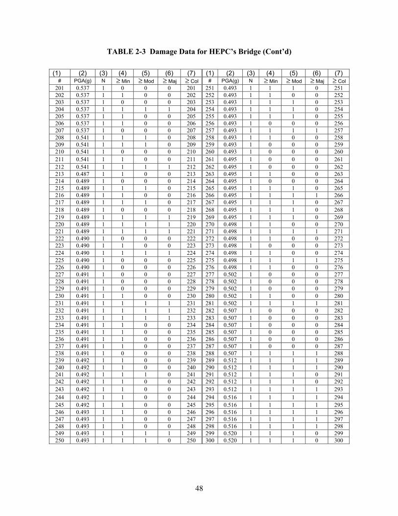
48
TABLE 2-3 Damage Data for HEPC’s Bridge (Cont’d)
(1) (2) (3) (4) (5) (6) (7) (1) (2) (3) (4) (5) (6) (7)
# PGA(g) N ≥ Min ≥ Mod ≥ Maj ≥ Col # PGA(g) N ≥ Min ≥ Mod ≥ Maj ≥ Col 201 0.537 1 0 0 0 201 251 0.493 1 1 1 0 251 202 0.537 1 1 0 0 202 252 0.493 1 1 0 0 252 203 0.537 1 0 0 0 203 253 0.493 1 1 1 0 253 204 0.537 1 1 1 1 204 254 0.493 1 1 1 0 254 205 0.537 1 1 0 0 205 255 0.493 1 1 1 0 255 206 0.537 1 1 0 0 206 256 0.493 1 0 0 0 256 207 0.537 1 0 0 0 207 257 0.493 1 1 1 1 257 208 0.541 1 1 1 0 208 258 0.493 1 1 0 0 258 209 0.541 1 1 1 0 209 259 0.493 1 0 0 0 259 210 0.541 1 0 0 0 210 260 0.493 1 0 0 0 260 211 0.541 1 1 0 0 211 261 0.495 1 0 0 0 261 212 0.541 1 1 1 1 212 262 0.495 1 0 0 0 262 213 0.487 1 1 0 0 213 263 0.495 1 1 0 0 263 214 0.489 1 0 0 0 214 264 0.495 1 0 0 0 264 215 0.489 1 1 1 0 215 265 0.495 1 1 1 0 265 216 0.489 1 1 0 0 216 266 0.495 1 1 1 1 266 217 0.489 1 1 1 0 217 267 0.495 1 1 1 0 267 218 0.489 1 0 0 0 218 268 0.495 1 1 1 0 268 219 0.489 1 1 1 1 219 269 0.495 1 1 1 0 269 220 0.489 1 1 1 1 220 270 0.498 1 1 0 0 270 221 0.489 1 1 1 1 221 271 0.498 1 1 1 1 271 222 0.490 1 0 0 0 222 272 0.498 1 1 0 0 272 223 0.490 1 1 0 0 223 273 0.498 1 0 0 0 273 224 0.490 1 1 1 1 224 274 0.498 1 1 0 0 274 225 0.490 1 0 0 0 225 275 0.498 1 1 1 1 275 226 0.490 1 0 0 0 226 276 0.498 1 1 0 0 276 227 0.491 1 0 0 0 227 277 0.502 1 0 0 0 277 228 0.491 1 0 0 0 228 278 0.502 1 0 0 0 278 229 0.491 1 0 0 0 229 279 0.502 1 0 0 0 279 230 0.491 1 1 0 0 230 280 0.502 1 1 0 0 280 231 0.491 1 1 1 1 231 281 0.502 1 1 1 1 281 232 0.491 1 1 1 1 232 282 0.507 1 0 0 0 282 233 0.491 1 1 1 1 233 283 0.507 1 0 0 0 283 234 0.491 1 1 0 0 234 284 0.507 1 0 0 0 284 235 0.491 1 1 0 0 235 285 0.507 1 0 0 0 285 236 0.491 1 1 0 0 236 286 0.507 1 0 0 0 286 237 0.491 1 1 0 0 237 287 0.507 1 0 0 0 287 238 0.491 1 0 0 0 238 288 0.507 1 1 1 1 288 239 0.492 1 1 0 0 239 289 0.512 1 1 1 1 289 240 0.492 1 1 0 0 240 290 0.512 1 1 1 1 290 241 0.492 1 1 1 0 241 291 0.512 1 1 1 0 291 242 0.492 1 1 0 0 242 292 0.512 1 1 1 0 292 243 0.492 1 1 0 0 243 293 0.512 1 1 1 1 293 244 0.492 1 1 0 0 244 294 0.516 1 1 1 1 294 245 0.492 1 1 0 0 245 295 0.516 1 1 1 1 295 246 0.493 1 1 0 0 246 296 0.516 1 1 1 1 296 247 0.493 1 1 0 0 247 297 0.516 1 1 1 1 297 248 0.493 1 1 0 0 248 298 0.516 1 1 1 1 298 249 0.493 1 1 1 1 249 299 0.520 1 1 1 0 299 250 0.493 1 1 1 0 250 300 0.520 1 1 1 0 300
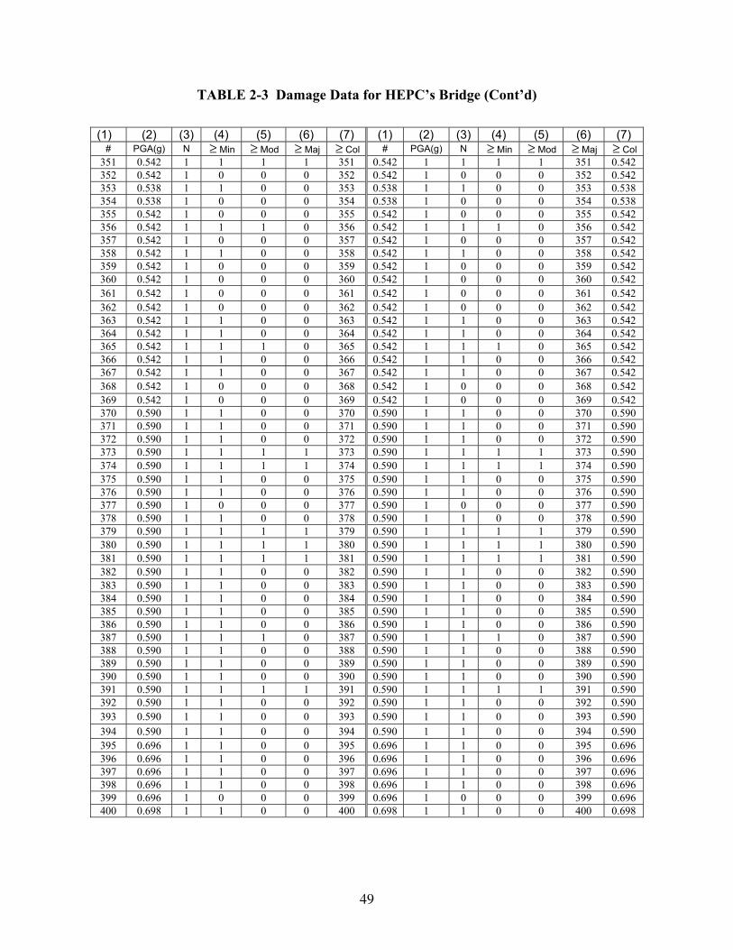
49
TABLE 2-3 Damage Data for HEPC’s Bridge (Cont’d)
(1) (2) (3) (4) (5) (6) (7) (1) (2) (3) (4) (5) (6) (7)
# PGA(g) N ≥ Min ≥ Mod ≥ Maj ≥ Col # PGA(g) N ≥ Min ≥ Mod ≥ Maj ≥ Col 351 0.542 1 1 1 1 351 0.542 1 1 1 1 351 0.542 352 0.542 1 0 0 0 352 0.542 1 0 0 0 352 0.542 353 0.538 1 1 0 0 353 0.538 1 1 0 0 353 0.538 354 0.538 1 0 0 0 354 0.538 1 0 0 0 354 0.538 355 0.542 1 0 0 0 355 0.542 1 0 0 0 355 0.542 356 0.542 1 1 1 0 356 0.542 1 1 1 0 356 0.542 357 0.542 1 0 0 0 357 0.542 1 0 0 0 357 0.542 358 0.542 1 1 0 0 358 0.542 1 1 0 0 358 0.542 359 0.542 1 0 0 0 359 0.542 1 0 0 0 359 0.542 360 0.542 1 0 0 0 360 0.542 1 0 0 0 360 0.542 361 0.542 1 0 0 0 361 0.542 1 0 0 0 361 0.542 362 0.542 1 0 0 0 362 0.542 1 0 0 0 362 0.542 363 0.542 1 1 0 0 363 0.542 1 1 0 0 363 0.542 364 0.542 1 1 0 0 364 0.542 1 1 0 0 364 0.542 365 0.542 1 1 1 0 365 0.542 1 1 1 0 365 0.542 366 0.542 1 1 0 0 366 0.542 1 1 0 0 366 0.542 367 0.542 1 1 0 0 367 0.542 1 1 0 0 367 0.542 368 0.542 1 0 0 0 368 0.542 1 0 0 0 368 0.542 369 0.542 1 0 0 0 369 0.542 1 0 0 0 369 0.542 370 0.590 1 1 0 0 370 0.590 1 1 0 0 370 0.590 371 0.590 1 1 0 0 371 0.590 1 1 0 0 371 0.590 372 0.590 1 1 0 0 372 0.590 1 1 0 0 372 0.590 373 0.590 1 1 1 1 373 0.590 1 1 1 1 373 0.590 374 0.590 1 1 1 1 374 0.590 1 1 1 1 374 0.590 375 0.590 1 1 0 0 375 0.590 1 1 0 0 375 0.590 376 0.590 1 1 0 0 376 0.590 1 1 0 0 376 0.590 377 0.590 1 0 0 0 377 0.590 1 0 0 0 377 0.590 378 0.590 1 1 0 0 378 0.590 1 1 0 0 378 0.590 379 0.590 1 1 1 1 379 0.590 1 1 1 1 379 0.590 380 0.590 1 1 1 1 380 0.590 1 1 1 1 380 0.590 381 0.590 1 1 1 1 381 0.590 1 1 1 1 381 0.590 382 0.590 1 1 0 0 382 0.590 1 1 0 0 382 0.590 383 0.590 1 1 0 0 383 0.590 1 1 0 0 383 0.590 384 0.590 1 1 0 0 384 0.590 1 1 0 0 384 0.590 385 0.590 1 1 0 0 385 0.590 1 1 0 0 385 0.590 386 0.590 1 1 0 0 386 0.590 1 1 0 0 386 0.590 387 0.590 1 1 1 0 387 0.590 1 1 1 0 387 0.590 388 0.590 1 1 0 0 388 0.590 1 1 0 0 388 0.590 389 0.590 1 1 0 0 389 0.590 1 1 0 0 389 0.590 390 0.590 1 1 0 0 390 0.590 1 1 0 0 390 0.590 391 0.590 1 1 1 1 391 0.590 1 1 1 1 391 0.590 392 0.590 1 1 0 0 392 0.590 1 1 0 0 392 0.590 393 0.590 1 1 0 0 393 0.590 1 1 0 0 393 0.590 394 0.590 1 1 0 0 394 0.590 1 1 0 0 394 0.590 395 0.696 1 1 0 0 395 0.696 1 1 0 0 395 0.696 396 0.696 1 1 0 0 396 0.696 1 1 0 0 396 0.696 397 0.696 1 1 0 0 397 0.696 1 1 0 0 397 0.696 398 0.696 1 1 0 0 398 0.696 1 1 0 0 398 0.696 399 0.696 1 0 0 0 399 0.696 1 0 0 0 399 0.696 400 0.698 1 1 0 0 400 0.698 1 1 0 0 400 0.698
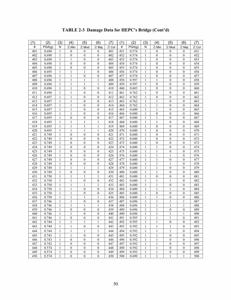
50
TABLE 2-3 Damage Data for HEPC’s Bridge (Cont’d)
(1) (2) (3) (4) (5) (6) (7) (1) (2) (3) (4) (5) (6) (7)
# PGA(g) N ≥ Min ≥ Mod ≥ Maj ≥ Col # PGA(g) N ≥ Min ≥ Mod ≥ Maj ≥ Col 401 0.698 1 0 0 0 401 451 0.574 1 0 0 0 451 402 0.698 1 0 0 0 402 452 0.574 1 0 0 0 452 403 0.698 1 1 0 0 403 453 0.574 1 0 0 0 453 404 0.698 1 0 0 0 404 454 0.574 1 0 0 0 454 405 0.698 1 0 0 0 405 455 0.574 1 0 0 0 455 406 0.695 1 1 1 0 406 456 0.574 1 0 0 0 456 407 0.696 1 1 0 0 407 457 0.574 1 0 0 0 457 408 0.696 1 1 1 1 408 458 0.597 1 1 0 0 458 409 0.696 1 1 1 1 409 459 0.597 1 0 0 0 459 410 0.696 1 1 0 0 410 460 0.603 1 0 0 0 460 411 0.696 1 1 0 0 411 461 0.762 1 0 0 0 461 412 0.697 1 1 0 0 412 462 0.762 1 0 0 0 462 413 0.697 1 1 0 0 413 463 0.762 1 1 0 0 463 414 0.697 1 1 0 0 414 464 0.762 1 1 0 0 464 415 0.697 1 1 0 0 415 465 0.600 1 1 0 0 465 416 0.695 1 1 0 0 416 466 0.600 1 0 0 0 466 417 0.695 1 0 0 0 417 467 0.600 1 1 0 0 467 418 0.695 1 1 1 1 418 468 0.600 1 1 0 0 468 419 0.695 1 1 1 1 419 469 0.600 1 0 0 0 469 420 0.695 1 1 1 1 420 470 0.600 1 0 0 0 470 421 0.749 1 0 0 0 421 471 0.600 1 0 0 0 471 422 0.749 1 0 0 0 422 472 0.600 1 0 0 0 472 423 0.749 1 0 0 0 423 473 0.600 1 0 0 0 473 424 0.749 1 0 0 0 424 474 0.600 1 1 0 0 474 425 0.749 1 0 0 0 425 475 0.600 1 1 0 0 475 426 0.749 1 0 0 0 426 476 0.600 1 1 1 0 476 427 0.749 1 0 0 0 427 477 0.600 1 1 0 0 477 428 0.749 1 0 0 0 428 478 0.600 1 1 1 0 478 429 0.749 1 1 1 1 429 479 0.600 1 1 0 0 479 430 0.749 1 0 0 0 430 480 0.600 1 1 0 0 480 431 0.750 1 1 1 1 431 481 0.600 1 0 0 0 481 432 0.750 1 1 0 0 432 482 0.600 1 1 1 0 482 433 0.750 1 1 1 1 433 483 0.600 1 1 0 0 483 434 0.750 1 1 0 0 434 484 0.600 1 1 1 0 484 435 0.750 1 1 0 0 435 485 0.600 1 0 0 0 485 436 0.750 1 1 1 1 436 486 0.600 1 1 0 0 486 437 0.746 1 1 0 0 437 487 0.696 1 1 1 1 487 438 0.746 1 1 1 1 438 488 0.696 1 1 1 1 488 439 0.746 1 0 0 0 439 489 0.696 1 1 0 0 489 440 0.746 1 1 0 0 440 490 0.696 1 1 1 1 490 441 0.746 1 0 0 0 441 491 0.595 1 1 1 0 491 442 0.744 1 1 1 1 442 492 0.595 1 1 0 0 492 443 0.744 1 1 0 0 443 493 0.592 1 1 1 0 493 444 0.744 1 1 1 1 444 494 0.592 1 1 1 0 494 445 0.743 1 1 0 0 445 495 0.592 1 1 0 0 495 446 0.743 1 0 0 0 446 496 0.592 1 1 0 0 496 447 0.742 1 0 0 0 447 497 0.592 1 1 0 0 497 448 0.574 1 0 0 0 448 498 0.592 1 1 0 0 498 449 0.574 1 0 0 0 449 499 0.592 1 1 0 0 499 450 0.574 1 0 0 0 450 500 0.690 1 1 1 1 500
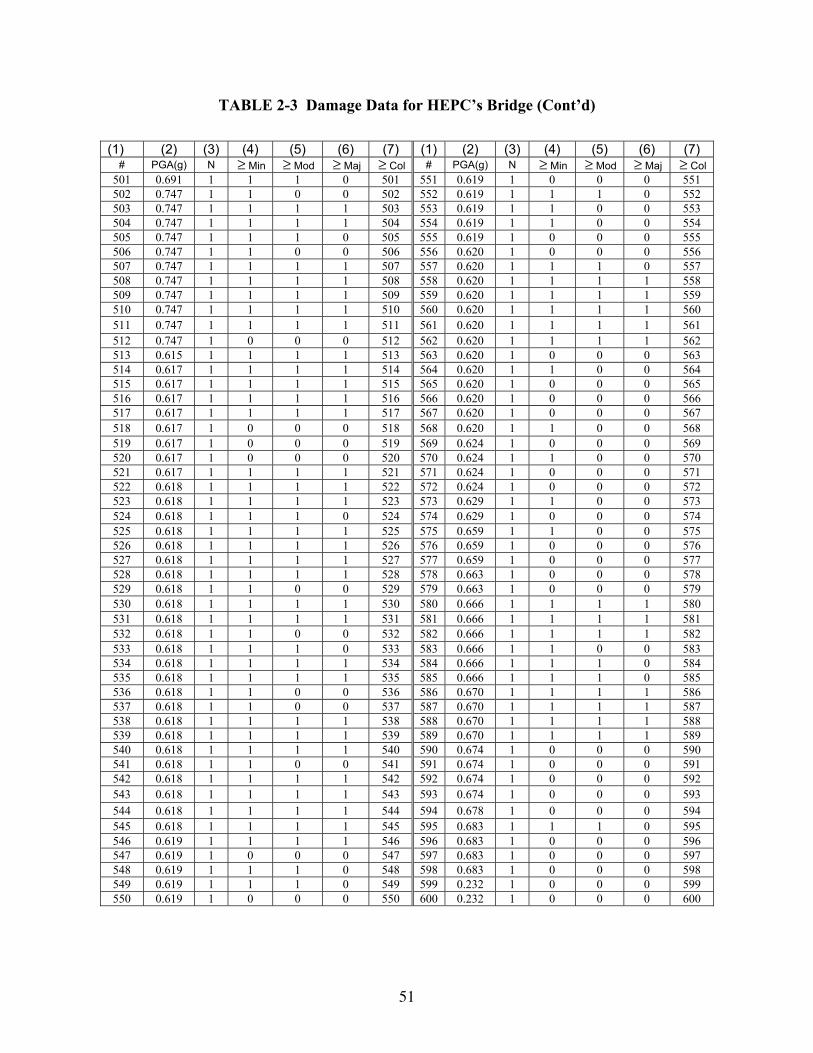
51
TABLE 2-3 Damage Data for HEPC’s Bridge (Cont’d)
(1) (2) (3) (4) (5) (6) (7) (1) (2) (3) (4) (5) (6) (7)
# PGA(g) N ≥ Min ≥ Mod ≥ Maj ≥ Col # PGA(g) N ≥ Min ≥ Mod ≥ Maj ≥ Col 501 0.691 1 1 1 0 501 551 0.619 1 0 0 0 551 502 0.747 1 1 0 0 502 552 0.619 1 1 1 0 552 503 0.747 1 1 1 1 503 553 0.619 1 1 0 0 553 504 0.747 1 1 1 1 504 554 0.619 1 1 0 0 554 505 0.747 1 1 1 0 505 555 0.619 1 0 0 0 555 506 0.747 1 1 0 0 506 556 0.620 1 0 0 0 556 507 0.747 1 1 1 1 507 557 0.620 1 1 1 0 557 508 0.747 1 1 1 1 508 558 0.620 1 1 1 1 558 509 0.747 1 1 1 1 509 559 0.620 1 1 1 1 559 510 0.747 1 1 1 1 510 560 0.620 1 1 1 1 560 511 0.747 1 1 1 1 511 561 0.620 1 1 1 1 561 512 0.747 1 0 0 0 512 562 0.620 1 1 1 1 562 513 0.615 1 1 1 1 513 563 0.620 1 0 0 0 563 514 0.617 1 1 1 1 514 564 0.620 1 1 0 0 564 515 0.617 1 1 1 1 515 565 0.620 1 0 0 0 565 516 0.617 1 1 1 1 516 566 0.620 1 0 0 0 566 517 0.617 1 1 1 1 517 567 0.620 1 0 0 0 567 518 0.617 1 0 0 0 518 568 0.620 1 1 0 0 568 519 0.617 1 0 0 0 519 569 0.624 1 0 0 0 569 520 0.617 1 0 0 0 520 570 0.624 1 1 0 0 570 521 0.617 1 1 1 1 521 571 0.624 1 0 0 0 571 522 0.618 1 1 1 1 522 572 0.624 1 0 0 0 572 523 0.618 1 1 1 1 523 573 0.629 1 1 0 0 573 524 0.618 1 1 1 0 524 574 0.629 1 0 0 0 574 525 0.618 1 1 1 1 525 575 0.659 1 1 0 0 575 526 0.618 1 1 1 1 526 576 0.659 1 0 0 0 576 527 0.618 1 1 1 1 527 577 0.659 1 0 0 0 577 528 0.618 1 1 1 1 528 578 0.663 1 0 0 0 578 529 0.618 1 1 0 0 529 579 0.663 1 0 0 0 579 530 0.618 1 1 1 1 530 580 0.666 1 1 1 1 580 531 0.618 1 1 1 1 531 581 0.666 1 1 1 1 581 532 0.618 1 1 0 0 532 582 0.666 1 1 1 1 582 533 0.618 1 1 1 0 533 583 0.666 1 1 0 0 583 534 0.618 1 1 1 1 534 584 0.666 1 1 1 0 584 535 0.618 1 1 1 1 535 585 0.666 1 1 1 0 585 536 0.618 1 1 0 0 536 586 0.670 1 1 1 1 586 537 0.618 1 1 0 0 537 587 0.670 1 1 1 1 587 538 0.618 1 1 1 1 538 588 0.670 1 1 1 1 588 539 0.618 1 1 1 1 539 589 0.670 1 1 1 1 589 540 0.618 1 1 1 1 540 590 0.674 1 0 0 0 590 541 0.618 1 1 0 0 541 591 0.674 1 0 0 0 591 542 0.618 1 1 1 1 542 592 0.674 1 0 0 0 592 543 0.618 1 1 1 1 543 593 0.674 1 0 0 0 593 544 0.618 1 1 1 1 544 594 0.678 1 0 0 0 594 545 0.618 1 1 1 1 545 595 0.683 1 1 1 0 595 546 0.619 1 1 1 1 546 596 0.683 1 0 0 0 596 547 0.619 1 0 0 0 547 597 0.683 1 0 0 0 597 548 0.619 1 1 1 0 548 598 0.683 1 0 0 0 598 549 0.619 1 1 1 0 549 599 0.232 1 0 0 0 599 550 0.619 1 0 0 0 550 600 0.232 1 0 0 0 600
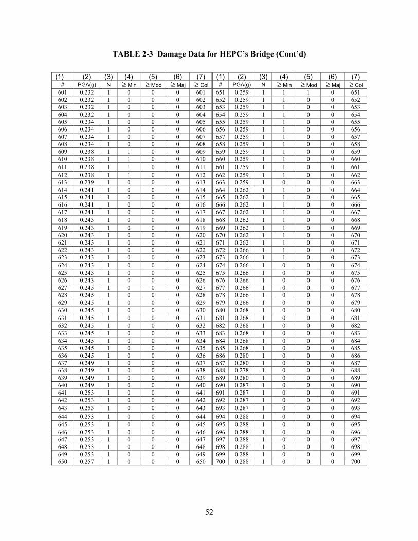
52
TABLE 2-3 Damage Data for HEPC’s Bridge (Cont’d)
(1) (2) (3) (4) (5) (6) (7) (1) (2) (3) (4) (5) (6) (7)
# PGA(g) N ≥ Min ≥ Mod ≥ Maj ≥ Col # PGA(g) N ≥ Min ≥ Mod ≥ Maj ≥ Col 601 0.232 1 0 0 0 601 651 0.259 1 1 1 0 651 602 0.232 1 0 0 0 602 652 0.259 1 1 0 0 652 603 0.232 1 0 0 0 603 653 0.259 1 1 0 0 653 604 0.232 1 0 0 0 604 654 0.259 1 1 0 0 654 605 0.234 1 0 0 0 605 655 0.259 1 1 0 0 655 606 0.234 1 0 0 0 606 656 0.259 1 1 0 0 656 607 0.234 1 0 0 0 607 657 0.259 1 1 0 0 657 608 0.234 1 0 0 0 608 658 0.259 1 1 0 0 658 609 0.238 1 1 0 0 609 659 0.259 1 1 0 0 659 610 0.238 1 1 0 0 610 660 0.259 1 1 0 0 660 611 0.238 1 1 0 0 611 661 0.259 1 1 0 0 661 612 0.238 1 1 0 0 612 662 0.259 1 1 0 0 662 613 0.239 1 0 0 0 613 663 0.259 1 0 0 0 663 614 0.241 1 0 0 0 614 664 0.262 1 1 0 0 664 615 0.241 1 0 0 0 615 665 0.262 1 1 0 0 665 616 0.241 1 0 0 0 616 666 0.262 1 1 0 0 666 617 0.241 1 0 0 0 617 667 0.262 1 1 0 0 667 618 0.243 1 0 0 0 618 668 0.262 1 1 0 0 668 619 0.243 1 0 0 0 619 669 0.262 1 1 0 0 669 620 0.243 1 0 0 0 620 670 0.262 1 1 0 0 670 621 0.243 1 0 0 0 621 671 0.262 1 1 0 0 671 622 0.243 1 0 0 0 622 672 0.266 1 1 0 0 672 623 0.243 1 0 0 0 623 673 0.266 1 1 0 0 673 624 0.243 1 0 0 0 624 674 0.266 1 0 0 0 674 625 0.243 1 0 0 0 625 675 0.266 1 0 0 0 675 626 0.243 1 0 0 0 626 676 0.266 1 0 0 0 676 627 0.245 1 0 0 0 627 677 0.266 1 0 0 0 677 628 0.245 1 0 0 0 628 678 0.266 1 0 0 0 678 629 0.245 1 0 0 0 629 679 0.266 1 0 0 0 679 630 0.245 1 0 0 0 630 680 0.268 1 0 0 0 680 631 0.245 1 0 0 0 631 681 0.268 1 0 0 0 681 632 0.245 1 0 0 0 632 682 0.268 1 0 0 0 682 633 0.245 1 0 0 0 633 683 0.268 1 0 0 0 683 634 0.245 1 0 0 0 634 684 0.268 1 0 0 0 684 635 0.245 1 0 0 0 635 685 0.268 1 0 0 0 685 636 0.245 1 0 0 0 636 686 0.280 1 0 0 0 686 637 0.249 1 0 0 0 637 687 0.280 1 0 0 0 687 638 0.249 1 0 0 0 638 688 0.278 1 0 0 0 688 639 0.249 1 0 0 0 639 689 0.280 1 0 0 0 689 640 0.249 1 0 0 0 640 690 0.287 1 0 0 0 690 641 0.253 1 0 0 0 641 691 0.287 1 0 0 0 691 642 0.253 1 0 0 0 642 692 0.287 1 0 0 0 692 643 0.253 1 0 0 0 643 693 0.287 1 0 0 0 693 644 0.253 1 0 0 0 644 694 0.288 1 0 0 0 694 645 0.253 1 0 0 0 645 695 0.288 1 0 0 0 695 646 0.253 1 0 0 0 646 696 0.288 1 0 0 0 696 647 0.253 1 0 0 0 647 697 0.288 1 0 0 0 697 648 0.253 1 0 0 0 648 698 0.288 1 0 0 0 698 649 0.253 1 0 0 0 649 699 0.288 1 0 0 0 699 650 0.257 1 0 0 0 650 700 0.288 1 0 0 0 700
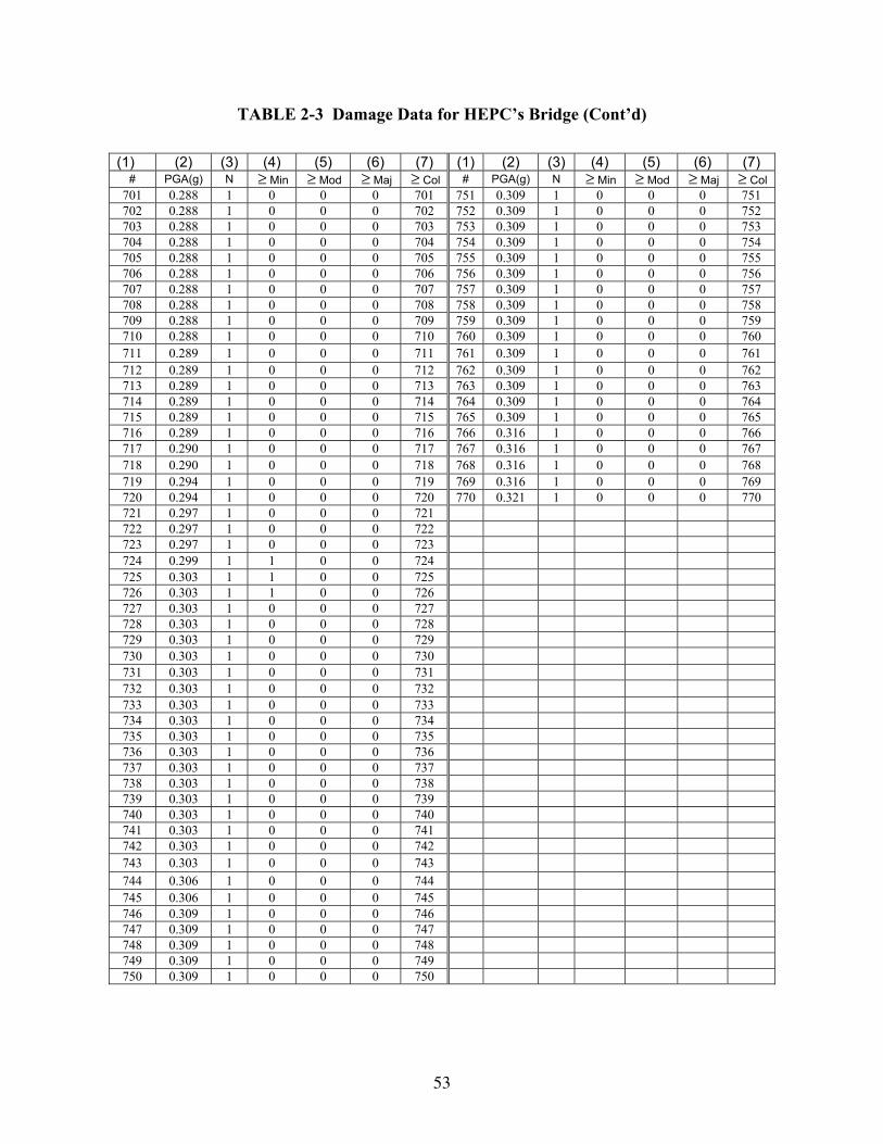
53
TABLE 2-3 Damage Data for HEPC’s Bridge (Cont’d)
(1) (2) (3) (4) (5) (6) (7) (1) (2) (3) (4) (5) (6) (7)
# PGA(g) N ≥ Min ≥ Mod ≥ Maj ≥ Col # PGA(g) N ≥ Min ≥ Mod ≥ Maj ≥ Col 701 0.288 1 0 0 0 701 751 0.309 1 0 0 0 751 702 0.288 1 0 0 0 702 752 0.309 1 0 0 0 752 703 0.288 1 0 0 0 703 753 0.309 1 0 0 0 753 704 0.288 1 0 0 0 704 754 0.309 1 0 0 0 754 705 0.288 1 0 0 0 705 755 0.309 1 0 0 0 755 706 0.288 1 0 0 0 706 756 0.309 1 0 0 0 756 707 0.288 1 0 0 0 707 757 0.309 1 0 0 0 757 708 0.288 1 0 0 0 708 758 0.309 1 0 0 0 758 709 0.288 1 0 0 0 709 759 0.309 1 0 0 0 759 710 0.288 1 0 0 0 710 760 0.309 1 0 0 0 760 711 0.289 1 0 0 0 711 761 0.309 1 0 0 0 761 712 0.289 1 0 0 0 712 762 0.309 1 0 0 0 762 713 0.289 1 0 0 0 713 763 0.309 1 0 0 0 763 714 0.289 1 0 0 0 714 764 0.309 1 0 0 0 764 715 0.289 1 0 0 0 715 765 0.309 1 0 0 0 765 716 0.289 1 0 0 0 716 766 0.316 1 0 0 0 766 717 0.290 1 0 0 0 717 767 0.316 1 0 0 0 767 718 0.290 1 0 0 0 718 768 0.316 1 0 0 0 768 719 0.294 1 0 0 0 719 769 0.316 1 0 0 0 769 720 0.294 1 0 0 0 720 770 0.321 1 0 0 0 770 721 0.297 1 0 0 0 721 722 0.297 1 0 0 0 722 723 0.297 1 0 0 0 723 724 0.299 1 1 0 0 724 725 0.303 1 1 0 0 725 726 0.303 1 1 0 0 726 727 0.303 1 0 0 0 727 728 0.303 1 0 0 0 728 729 0.303 1 0 0 0 729 730 0.303 1 0 0 0 730 731 0.303 1 0 0 0 731 732 0.303 1 0 0 0 732 733 0.303 1 0 0 0 733 734 0.303 1 0 0 0 734 735 0.303 1 0 0 0 735 736 0.303 1 0 0 0 736 737 0.303 1 0 0 0 737 738 0.303 1 0 0 0 738 739 0.303 1 0 0 0 739 740 0.303 1 0 0 0 740 741 0.303 1 0 0 0 741 742 0.303 1 0 0 0 742 743 0.303 1 0 0 0 743 744 0.306 1 0 0 0 744 745 0.306 1 0 0 0 745 746 0.309 1 0 0 0 746 747 0.309 1 0 0 0 747 748 0.309 1 0 0 0 748 749 0.309 1 0 0 0 749 750 0.309 1 0 0 0 750
54
2.4 Fragility Curves for Structural Sub-Sets of Caltrans’ Bridges
In the preceding analysis, it was assumed that the sample of bridges inspected after the
earthquake is statistically homogeneous. This assumption is not quite reasonable for the
Caltrans’ bridges, while it is reasonable for the HEPC’s bridge columns as mentioned earlier. In
the present study, therefore, the sample of the HEPC’s bridge columns considered is treated
statistically as homogeneous and figures 2-16 and 2-17 represent the families of fragility curves
assignable to any bridge column arbitrarily chosen from the underlying homogenous population
of bridge columns. For the mathematical reasons mentioned earlier, it is recommended even
then that the fragility curves (figure 2-17) obtained by means of Method 2 be considered for
applications, although later statistical analysis will indicate that the fragility curves (figure 2-16)
obtained by Method 1 cannot mathematically be rejected. As opposed to the case of HEPC’s
bridge columns, the statistical homogeneity would be an oversimplification for the sample of the
Caltrans’ bridges. In fact, it is reasonable to sub-divide the sample of the Caltrans’ bridges into a
number of sub-sets in accordance with the pertinent bridge attributes and their combinations.
This should be done in such a way that each sub-sample can be considered to be drawn from the
corresponding sub-population which is more homogeneous than the initial population. In this
regard, it is recognized each bridge can easily be associated with one of the following three
distinct attributes; (A) It is either single span (S) or multiple span (M) bridge, (B) it is built on
either hard soil (S1), medium soil (S2) or soft soil (S3) in the definition of UBC 93, and (C) it has
a skew angle 1θ (less than o20 ), 2θ (between o20 and o60 ) or 3θ (larger than o60 ). The
sample can then be sub-divided into a number of sub-sets. To begin with, one might consider the
first level hypothesis that the entire sample is taken from a statistically homogenous population
of bridges. The second level sub-sets are created by dividing the sample either (A) into two
groups of bridges, one with single spans and the other with multiple spans, (B) into three groups,
the first with soil condition S1, the second with S2 and the third with S3, or (C) into three groups
depending on the skew angles 1θ , 2θ and 3θ . The third level sub-sets consists of either (D) 6
groups each with a particular combination between (S, M) and (S1, S2, S3), (E) 6 groups each
with a combination between (S, M) and ( 1θ , 2θ , 3θ ), or (F) 9 groups each with a combination
55
between ( 1θ , 2θ , 3θ ) and (S1, S2, S3). Finally, the fourth level sub-sets comprises of 18 groups
each with a combination of the attributes (S, M), (S1, S2, S3) and ( 1θ , 2θ , 3θ ).
As alluded to in the preceding paragraph, the higher the level of sub-sets, more statistically
homogeneous the corresponding sub-population is compared with the population at the level at
least one rank lower. For example, each sample of the fourth level sub-sets is taken from the
population with identical span, skewness and soil characteristics as they are defined here. While
this by no means implies that the corresponding population is purely homogeneous, it is much
more homogeneous in engineering sense than the population corresponding to the first, second or
even third level sub-sets.
The first level represents nothing but the entire sample taken from the underlying homogeneous
population. The fragility curves are developed under this assumption in figures 2-3 and 2-4 for
the Caltrans’ bridges. The second, third and fourth level sub-sets are all considered and analyzed
for the fragility curve development with the aid of Method 2. The median values and log-
standard deviations of all levels of attribute combinations are listed in table 2-4. Note that, if an
element of a matrix in table 2-4 shows NA, it indicates that null sub-sample was found for the
particular combination of bridge attributes the element signifies. The families of fragility curves
corresponding to the fourth level subsets consisting of 18 groups are plotted in figures 2-24~2-36.
Fragility curves associated with some damage states are missing from the plots for some subsets
that do not have bridges suffering from these damage states. For example, the subset
representing the combination of bridge attributes M/ 1θ / a (multiple span/skew angle between 0
and o20 /soil condition A) does not have empirical fragility curves for at least major and collapse
states of damage (see table 2-4). Also, there exist, at the fourth level of subdivision, five empty
subsets (S/20~60/a, S/20~60/b, S/60~90/a, S/60~90/b, M/0~20/b) for which these are no
empirical fragility curves at all. The higher the level of sub-sets, fragility curves obtained by
Method 1 tend to more easily to intersect each other when they are plotted within the same
family having a specific combination of attributes because of the smaller sample size it tends to
consist of. A typical example of this is shown in figure 2-37. This indeed is the reason for not

56
utilizing the fragility curves developed at level four by Method 1 in the ensuing system
performance analysis.
The families of fragility curves shown in figures 2-24~2-36 play a pivotal role in the seismic
performance assessment of the expressway network in the Los Angeles area. More will be
mentioned about this later in this report.
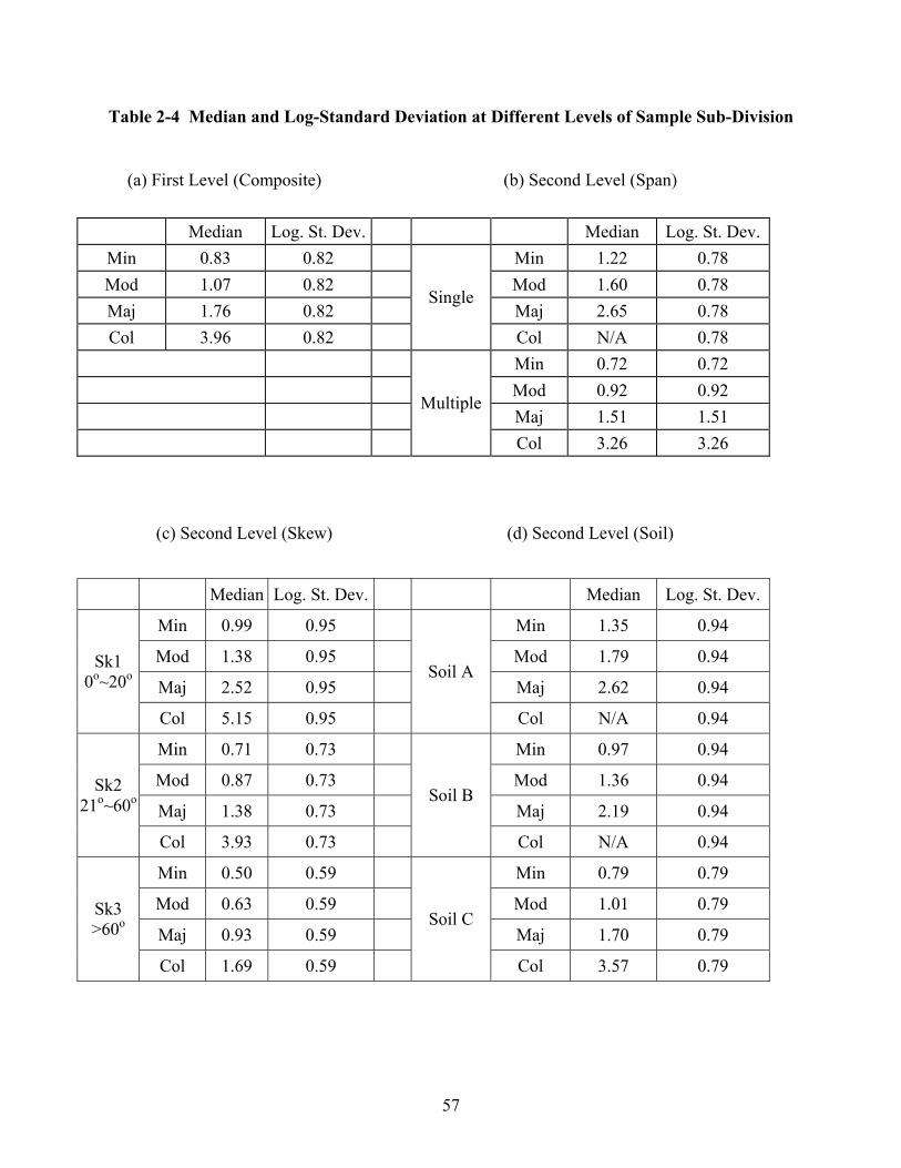
57
Table 2-4 Median and Log-Standard Deviation at Different Levels of Sample Sub-Division
(a) First Level (Composite) (b) Second Level (Span)
Median Log. St. Dev. Median Log. St. Dev.Min 0.83 0.82 Min 1.22 0.78 Mod 1.07 0.82 Mod 1.60 0.78 Maj 1.76 0.82 Maj 2.65 0.78 Col 3.96 0.82
Single
Col N/A 0.78 Min 0.72 0.72 Mod 0.92 0.92 Maj 1.51 1.51
Multiple
Col 3.26 3.26
(c) Second Level (Skew) (d) Second Level (Soil)
Median Log. St. Dev. Median Log. St. Dev.
Min 0.99 0.95 Min 1.35 0.94
Mod 1.38 0.95 Mod 1.79 0.94
Maj 2.52 0.95 Maj 2.62 0.94 Sk1
0o~20o
Col 5.15 0.95
Soil A
Col N/A 0.94
Min 0.71 0.73 Min 0.97 0.94
Mod 0.87 0.73 Mod 1.36 0.94
Maj 1.38 0.73 Maj 2.19 0.94 Sk2
21o~60o
Col 3.93 0.73
Soil B
Col N/A 0.94
Min 0.50 0.59 Min 0.79 0.79
Mod 0.63 0.59 Mod 1.01 0.79
Maj 0.93 0.59 Maj 1.70 0.79 Sk3 >60o
Col 1.69 0.59
Soil C
Col 3.57 0.79
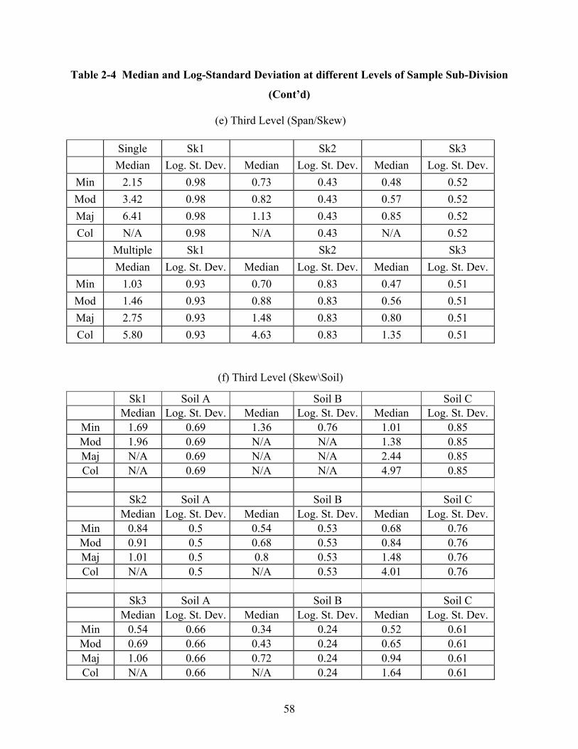
58
Table 2-4 Median and Log-Standard Deviation at different Levels of Sample Sub-Division
(Cont’d)
(e) Third Level (Span/Skew)
Single Sk1 Sk2 Sk3 Median Log. St. Dev. Median Log. St. Dev. Median Log. St. Dev.
Min 2.15 0.98 0.73 0.43 0.48 0.52 Mod 3.42 0.98 0.82 0.43 0.57 0.52 Maj 6.41 0.98 1.13 0.43 0.85 0.52 Col N/A 0.98 N/A 0.43 N/A 0.52
Multiple Sk1 Sk2 Sk3 Median Log. St. Dev. Median Log. St. Dev. Median Log. St. Dev.
Min 1.03 0.93 0.70 0.83 0.47 0.51 Mod 1.46 0.93 0.88 0.83 0.56 0.51 Maj 2.75 0.93 1.48 0.83 0.80 0.51 Col 5.80 0.93 4.63 0.83 1.35 0.51
(f) Third Level (Skew\Soil)
Sk1 Soil A Soil B Soil C Median Log. St. Dev. Median Log. St. Dev. Median Log. St. Dev.
Min 1.69 0.69 1.36 0.76 1.01 0.85 Mod 1.96 0.69 N/A N/A 1.38 0.85 Maj N/A 0.69 N/A N/A 2.44 0.85 Col N/A 0.69 N/A N/A 4.97 0.85
Sk2 Soil A Soil B Soil C Median Log. St. Dev. Median Log. St. Dev. Median Log. St. Dev.
Min 0.84 0.5 0.54 0.53 0.68 0.76 Mod 0.91 0.5 0.68 0.53 0.84 0.76 Maj 1.01 0.5 0.8 0.53 1.48 0.76 Col N/A 0.5 N/A 0.53 4.01 0.76
Sk3 Soil A Soil B Soil C Median Log. St. Dev. Median Log. St. Dev. Median Log. St. Dev.
Min 0.54 0.66 0.34 0.24 0.52 0.61 Mod 0.69 0.66 0.43 0.24 0.65 0.61 Maj 1.06 0.66 0.72 0.24 0.94 0.61 Col N/A 0.66 N/A 0.24 1.64 0.61
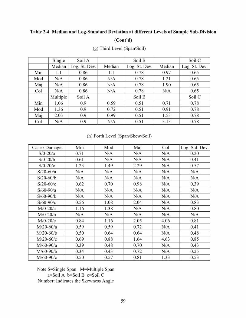
59
Table 2-4 Median and Log-Standard Deviation at different Levels of Sample Sub-Division
(Cont’d)
(g) Third Level (Span\Soil)
Single Soil A Soil B Soil C Median Log. St. Dev. Median Log. St. Dev. Median Log. St. Dev.
Min 1.1 0.86 1.1 0.78 0.97 0.65 Mod N/A 0.86 N/A 0.78 1.21 0.65 Maj N/A 0.86 N/A 0.78 1.90 0.65 Col N/A 0.86 N/A 0.78 N/A 0.65
Multiple Soil A Soil B Soil C Min 1.06 0.9 0.59 0.51 0.71 0.78 Mod 1.36 0.9 0.72 0.51 0.91 0.78 Maj 2.03 0.9 0.99 0.51 1.53 0.78 Col N/A 0.9 N/A 0.51 3.13 0.78
(h) Forth Level (Span/Skew/Soil)
Case \ Damage Min Mod Maj Col Log. Std. Dev.S/0-20/a 0.71 N/A N/A N/A 0.20 S/0-20/b 0.61 N/A N/A N/A 0.41 S/0-20/c 1.23 1.49 2.29 N/A 0.57 S/20-60/a N/A N/A N/A N/A N/A S/20-60/b N/A N/A N/A N/A N/A S/20-60/c 0.62 0.70 0.98 N/A 0.39 S/60-90/a N/A N/A N/A N/A N/A S/60-90/b N/A N/A N/A N/A N/A S/60-90/c 0.56 1.08 2.04 N/A 0.83 M/0-20/a 1.16 1.38 N/A N/A 0.80 M/0-20/b N/A N/A N/A N/A N/A M/0-20/c 0.84 1.16 2.05 4.06 0.81 M/20-60/a 0.59 0.59 0.72 N/A 0.41 M/20-60/b 0.50 0.64 0.64 N/A 0.48 M/20-60/c 0.69 0.88 1.64 4.63 0.85 M/60-90/a 0.39 0.48 0.70 N/A 0.43 M/60-90/b 0.34 0.43 0.72 N/A 0.25 M/60-90/c 0.50 0.57 0.81 1.33 0.53
Note S=Single Span M=Multiple Span
a=Soil A b=Soil B c=Soil C Number: Indicates the Skewness Angle
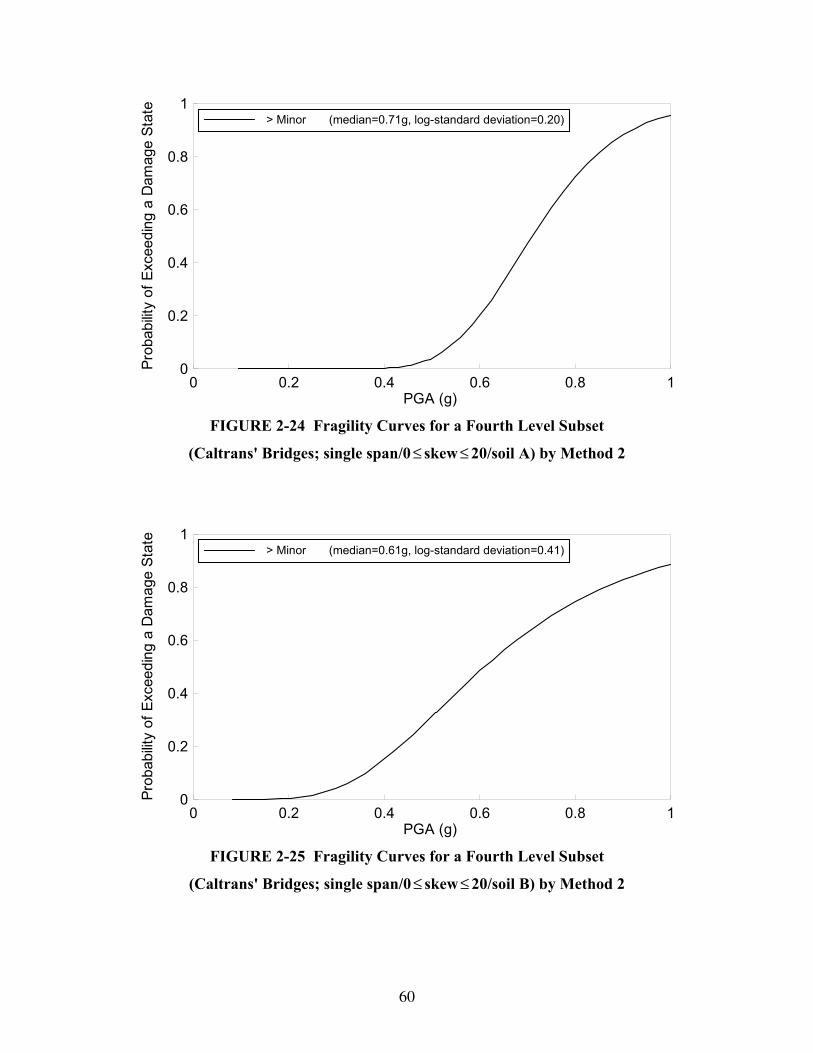
60
0 0.2 0.4 0.6 0.8 1PGA (g)
0
0.2
0.4
0.6
0.8
1
Prob
abilit
y of
Exc
eedi
ng a
Dam
age
Stat
e
> Minor (median=0.71g, log-standard deviation=0.20)
FIGURE 2-24 Fragility Curves for a Fourth Level Subset
(Caltrans' Bridges; single span/0 ≤ skew ≤ 20/soil A) by Method 2
0 0.2 0.4 0.6 0.8 1PGA (g)
0
0.2
0.4
0.6
0.8
1
Prob
abilit
y of
Exc
eedi
ng a
Dam
age
Stat
e
> Minor (median=0.61g, log-standard deviation=0.41)
FIGURE 2-25 Fragility Curves for a Fourth Level Subset
(Caltrans' Bridges; single span/0 ≤ skew ≤ 20/soil B) by Method 2
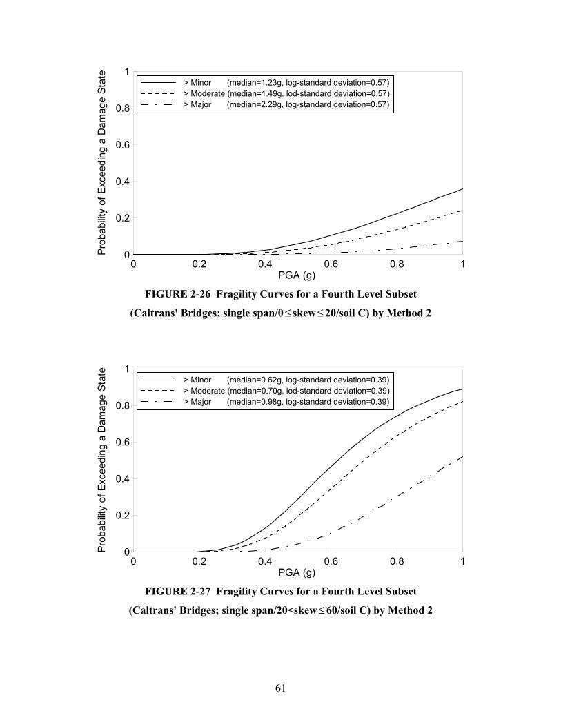
61
0 0.2 0.4 0.6 0.8 1PGA (g)
0
0.2
0.4
0.6
0.8
1
Prob
abilit
y of
Exc
eedi
ng a
Dam
age
Stat
e
> Minor (median=1.23g, log-standard deviation=0.57) > Moderate (median=1.49g, lod-standard deviation=0.57) > Major (median=2.29g, log-standard deviation=0.57)
FIGURE 2-26 Fragility Curves for a Fourth Level Subset
(Caltrans' Bridges; single span/0 ≤ skew ≤ 20/soil C) by Method 2
0 0.2 0.4 0.6 0.8 1PGA (g)
0
0.2
0.4
0.6
0.8
1
Prob
abilit
y of
Exc
eedi
ng a
Dam
age
Stat
e
> Minor (median=0.62g, log-standard deviation=0.39) > Moderate (median=0.70g, lod-standard deviation=0.39) > Major (median=0.98g, log-standard deviation=0.39)
FIGURE 2-27 Fragility Curves for a Fourth Level Subset
(Caltrans' Bridges; single span/20<skew ≤ 60/soil C) by Method 2
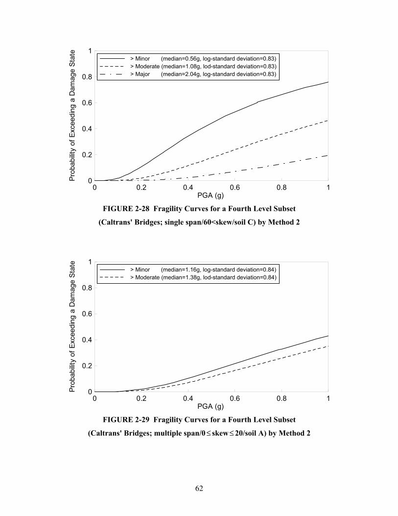
62
0 0.2 0.4 0.6 0.8 1PGA (g)
0
0.2
0.4
0.6
0.8
1
Prob
abilit
y of
Exc
eedi
ng a
Dam
age
Stat
e
> Minor (median=0.56g, log-standard deviation=0.83) > Moderate (median=1.08g, lod-standard deviation=0.83) > Major (median=2.04g, log-standard deviation=0.83)
FIGURE 2-28 Fragility Curves for a Fourth Level Subset
(Caltrans' Bridges; single span/60<skew/soil C) by Method 2
0 0.2 0.4 0.6 0.8 1PGA (g)
0
0.2
0.4
0.6
0.8
1
Prob
abilit
y of
Exc
eedi
ng a
Dam
age
Stat
e
> Minor (median=1.16g, log-standard deviation=0.84) > Moderate (median=1.38g, lod-standard deviation=0.84)
FIGURE 2-29 Fragility Curves for a Fourth Level Subset
(Caltrans' Bridges; multiple span/0 ≤ skew ≤ 20/soil A) by Method 2
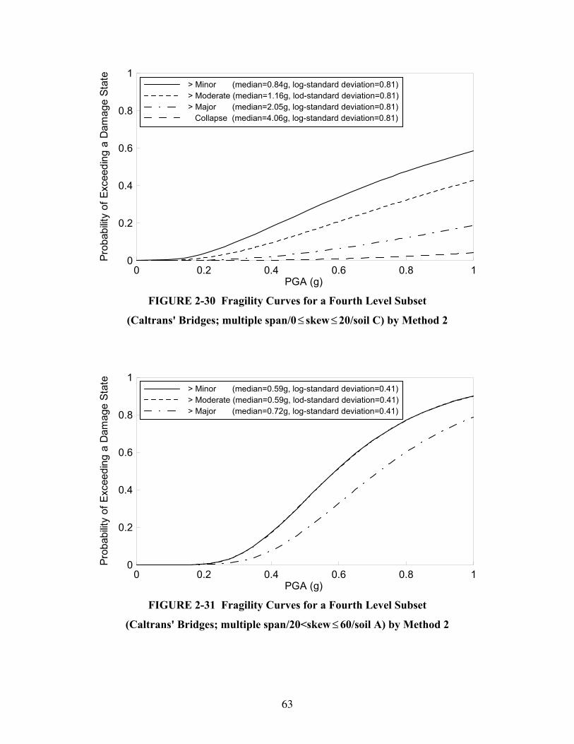
63
0 0.2 0.4 0.6 0.8 1PGA (g)
0
0.2
0.4
0.6
0.8
1
Prob
abilit
y of
Exc
eedi
ng a
Dam
age
Stat
e
> Minor (median=0.84g, log-standard deviation=0.81) > Moderate (median=1.16g, lod-standard deviation=0.81) > Major (median=2.05g, log-standard deviation=0.81) Collapse (median=4.06g, log-standard deviation=0.81)
FIGURE 2-30 Fragility Curves for a Fourth Level Subset
(Caltrans' Bridges; multiple span/0 ≤ skew ≤ 20/soil C) by Method 2
0 0.2 0.4 0.6 0.8 1PGA (g)
0
0.2
0.4
0.6
0.8
1
Prob
abilit
y of
Exc
eedi
ng a
Dam
age
Stat
e
> Minor (median=0.59g, log-standard deviation=0.41) > Moderate (median=0.59g, lod-standard deviation=0.41) > Major (median=0.72g, log-standard deviation=0.41)
FIGURE 2-31 Fragility Curves for a Fourth Level Subset
(Caltrans' Bridges; multiple span/20<skew ≤ 60/soil A) by Method 2
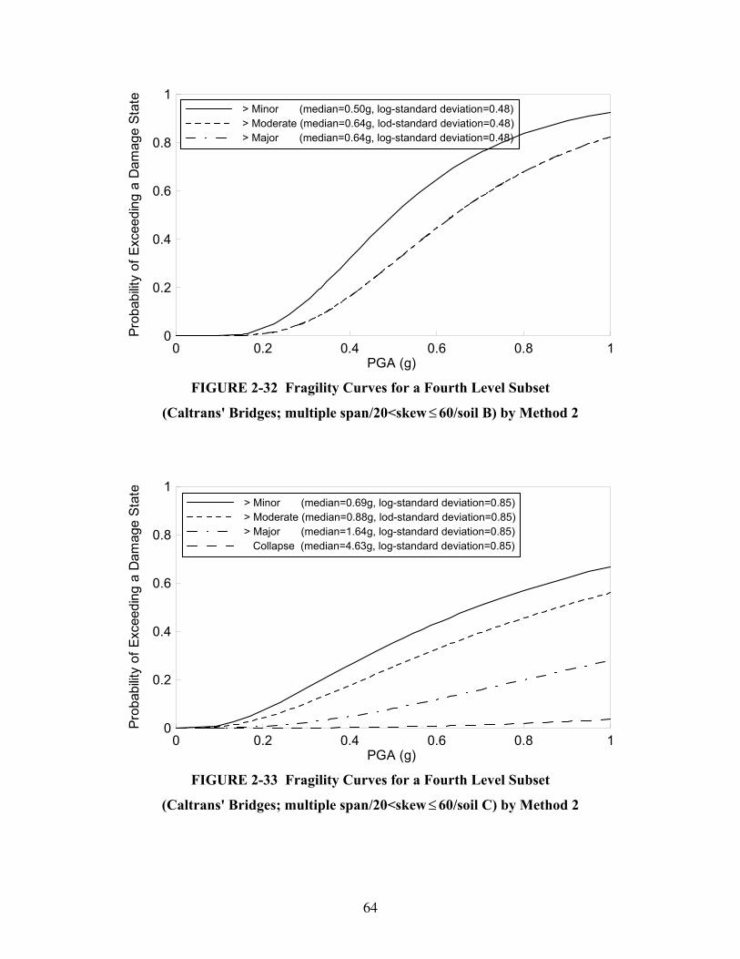
64
0 0.2 0.4 0.6 0.8 1PGA (g)
0
0.2
0.4
0.6
0.8
1
Prob
abilit
y of
Exc
eedi
ng a
Dam
age
Stat
e
> Minor (median=0.50g, log-standard deviation=0.48) > Moderate (median=0.64g, lod-standard deviation=0.48) > Major (median=0.64g, log-standard deviation=0.48)
FIGURE 2-32 Fragility Curves for a Fourth Level Subset
(Caltrans' Bridges; multiple span/20<skew ≤ 60/soil B) by Method 2
0 0.2 0.4 0.6 0.8 1PGA (g)
0
0.2
0.4
0.6
0.8
1
Prob
abilit
y of
Exc
eedi
ng a
Dam
age
Stat
e
> Minor (median=0.69g, log-standard deviation=0.85) > Moderate (median=0.88g, lod-standard deviation=0.85) > Major (median=1.64g, log-standard deviation=0.85) Collapse (median=4.63g, log-standard deviation=0.85)
FIGURE 2-33 Fragility Curves for a Fourth Level Subset
(Caltrans' Bridges; multiple span/20<skew ≤ 60/soil C) by Method 2
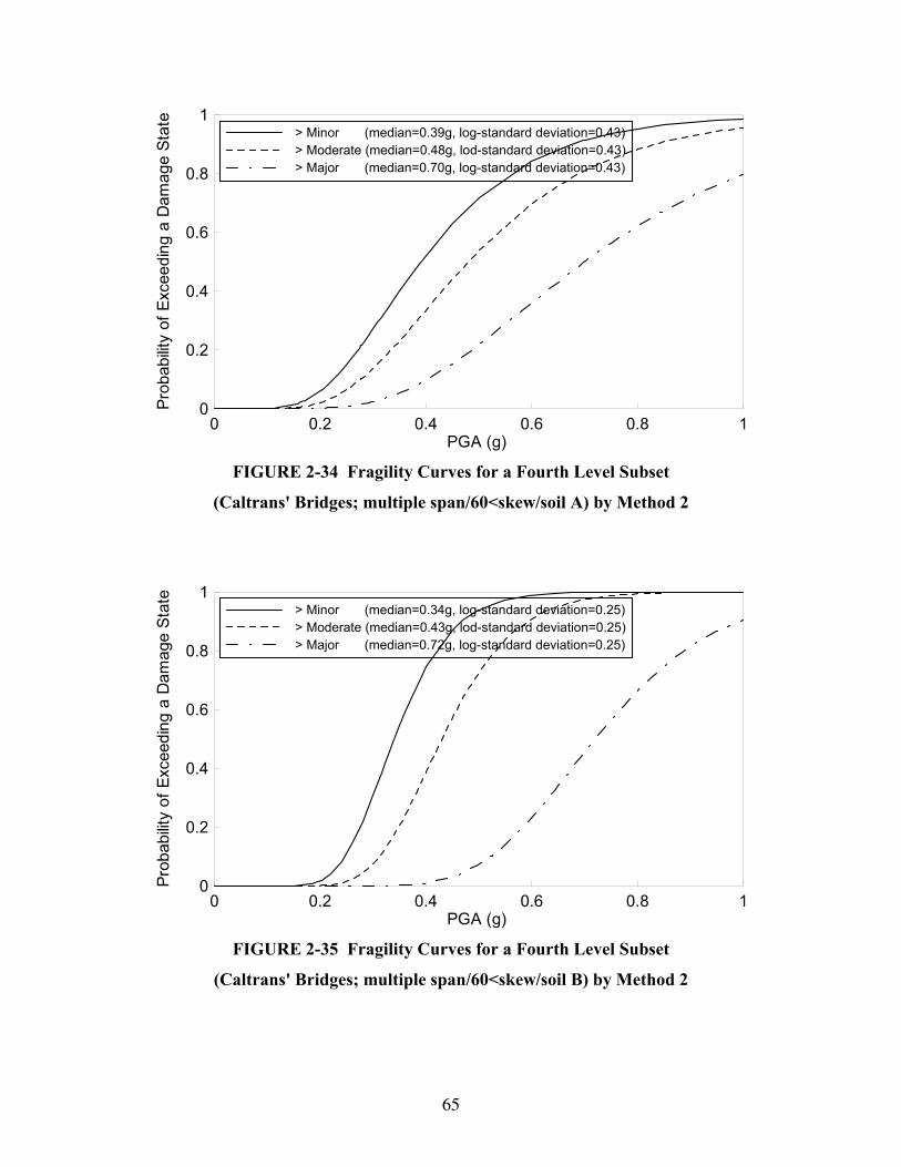
65
0 0.2 0.4 0.6 0.8 1PGA (g)
0
0.2
0.4
0.6
0.8
1
Prob
abilit
y of
Exc
eedi
ng a
Dam
age
Stat
e
> Minor (median=0.39g, log-standard deviation=0.43) > Moderate (median=0.48g, lod-standard deviation=0.43) > Major (median=0.70g, log-standard deviation=0.43)
FIGURE 2-34 Fragility Curves for a Fourth Level Subset
(Caltrans' Bridges; multiple span/60<skew/soil A) by Method 2
0 0.2 0.4 0.6 0.8 1PGA (g)
0
0.2
0.4
0.6
0.8
1
Prob
abilit
y of
Exc
eedi
ng a
Dam
age
Stat
e
> Minor (median=0.34g, log-standard deviation=0.25) > Moderate (median=0.43g, lod-standard deviation=0.25) > Major (median=0.72g, log-standard deviation=0.25)
FIGURE 2-35 Fragility Curves for a Fourth Level Subset
(Caltrans' Bridges; multiple span/60<skew/soil B) by Method 2
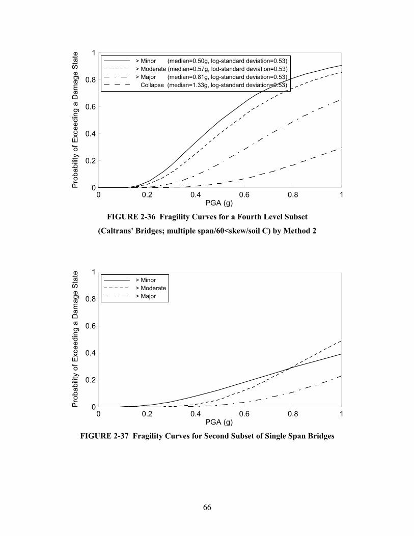
66
0 0.2 0.4 0.6 0.8 1PGA (g)
0
0.2
0.4
0.6
0.8
1
Prob
abilit
y of
Exc
eedi
ng a
Dam
age
Stat
e
> Minor (median=0.50g, log-standard deviation=0.53) > Moderate (median=0.57g, lod-standard deviation=0.53) > Major (median=0.81g, log-standard deviation=0.53) Collapse (median=1.33g, log-standard deviation=0.53)
FIGURE 2-36 Fragility Curves for a Fourth Level Subset
(Caltrans' Bridges; multiple span/60<skew/soil C) by Method 2
0 0.2 0.4 0.6 0.8 1PGA (g)
0
0.2
0.4
0.6
0.8
1
Prob
abilit
y of
Exc
eedi
ng a
Dam
age
Stat
e
> Minor > Moderate > Major
FIGURE 2-37 Fragility Curves for Second Subset of Single Span Bridges
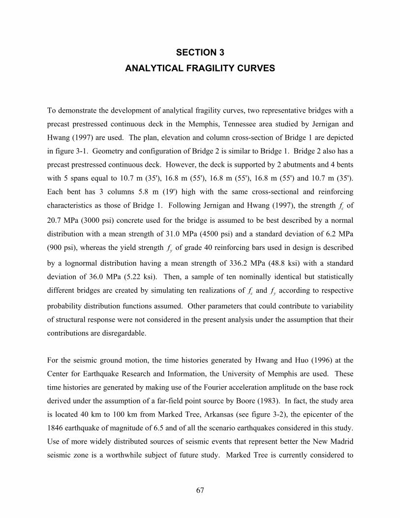
67
SECTION 3 ANALYTICAL FRAGILITY CURVES
To demonstrate the development of analytical fragility curves, two representative bridges with a
precast prestressed continuous deck in the Memphis, Tennessee area studied by Jernigan and
Hwang (1997) are used. The plan, elevation and column cross-section of Bridge 1 are depicted
in figure 3-1. Geometry and configuration of Bridge 2 is similar to Bridge 1. Bridge 2 also has a
precast prestressed continuous deck. However, the deck is supported by 2 abutments and 4 bents
with 5 spans equal to 10.7 m (35'), 16.8 m (55'), 16.8 m (55'), 16.8 m (55') and 10.7 m (35').
Each bent has 3 columns 5.8 m (19') high with the same cross-sectional and reinforcing
characteristics as those of Bridge 1. Following Jernigan and Hwang (1997), the strength fc of
20.7 MPa (3000 psi) concrete used for the bridge is assumed to be best described by a normal
distribution with a mean strength of 31.0 MPa (4500 psi) and a standard deviation of 6.2 MPa
(900 psi), whereas the yield strength fy of grade 40 reinforcing bars used in design is described
by a lognormal distribution having a mean strength of 336.2 MPa (48.8 ksi) with a standard
deviation of 36.0 MPa (5.22 ksi). Then, a sample of ten nominally identical but statistically
different bridges are created by simulating ten realizations of fc and fy according to respective
probability distribution functions assumed. Other parameters that could contribute to variability
of structural response were not considered in the present analysis under the assumption that their
contributions are disregardable.
For the seismic ground motion, the time histories generated by Hwang and Huo (1996) at the
Center for Earthquake Research and Information, the University of Memphis are used. These
time histories are generated by making use of the Fourier acceleration amplitude on the base rock
derived under the assumption of a far-field point source by Boore (1983). In fact, the study area
is located 40 km to 100 km from Marked Tree, Arkansas (see figure 3-2), the epicenter of the
1846 earthquake of magnitude of 6.5 and of all the scenario earthquakes considered in this study.
Use of more widely distributed sources of seismic events that represent better the New Madrid
seismic zone is a worthwhile subject of future study. Marked Tree is currently considered to
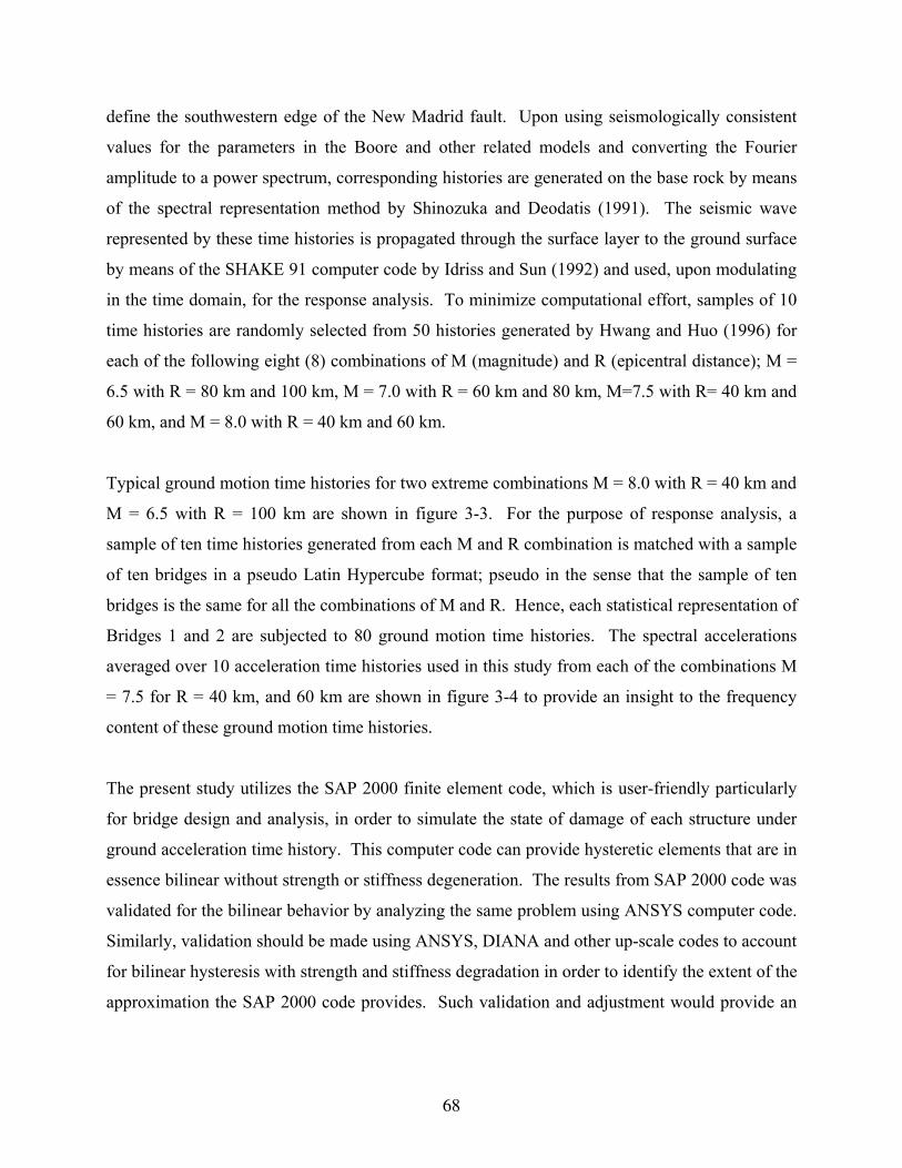
68
define the southwestern edge of the New Madrid fault. Upon using seismologically consistent
values for the parameters in the Boore and other related models and converting the Fourier
amplitude to a power spectrum, corresponding histories are generated on the base rock by means
of the spectral representation method by Shinozuka and Deodatis (1991). The seismic wave
represented by these time histories is propagated through the surface layer to the ground surface
by means of the SHAKE 91 computer code by Idriss and Sun (1992) and used, upon modulating
in the time domain, for the response analysis. To minimize computational effort, samples of 10
time histories are randomly selected from 50 histories generated by Hwang and Huo (1996) for
each of the following eight (8) combinations of M (magnitude) and R (epicentral distance); M =
6.5 with R = 80 km and 100 km, M = 7.0 with R = 60 km and 80 km, M=7.5 with R= 40 km and
60 km, and M = 8.0 with R = 40 km and 60 km.
Typical ground motion time histories for two extreme combinations M = 8.0 with R = 40 km and
M = 6.5 with R = 100 km are shown in figure 3-3. For the purpose of response analysis, a
sample of ten time histories generated from each M and R combination is matched with a sample
of ten bridges in a pseudo Latin Hypercube format; pseudo in the sense that the sample of ten
bridges is the same for all the combinations of M and R. Hence, each statistical representation of
Bridges 1 and 2 are subjected to 80 ground motion time histories. The spectral accelerations
averaged over 10 acceleration time histories used in this study from each of the combinations M
= 7.5 for R = 40 km, and 60 km are shown in figure 3-4 to provide an insight to the frequency
content of these ground motion time histories.
The present study utilizes the SAP 2000 finite element code, which is user-friendly particularly
for bridge design and analysis, in order to simulate the state of damage of each structure under
ground acceleration time history. This computer code can provide hysteretic elements that are in
essence bilinear without strength or stiffness degeneration. The results from SAP 2000 code was
validated for the bilinear behavior by analyzing the same problem using ANSYS computer code.
Similarly, validation should be made using ANSYS, DIANA and other up-scale codes to account
for bilinear hysteresis with strength and stiffness degradation in order to identify the extent of the
approximation the SAP 2000 code provides. Such validation and adjustment would provide an
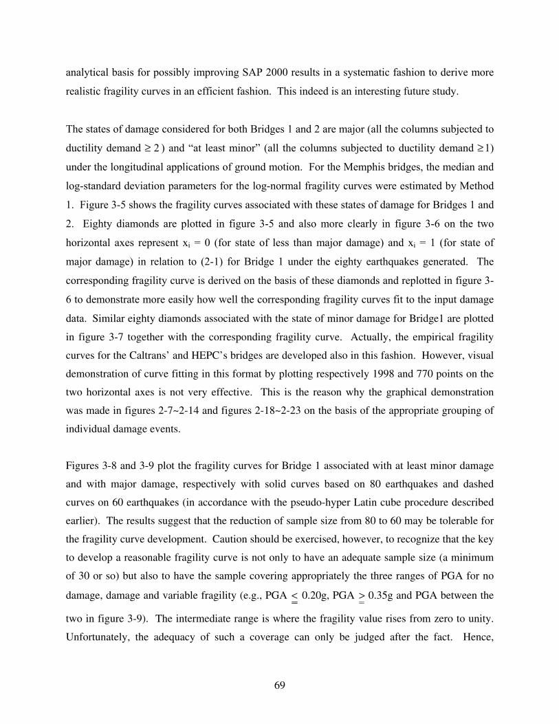
69
analytical basis for possibly improving SAP 2000 results in a systematic fashion to derive more
realistic fragility curves in an efficient fashion. This indeed is an interesting future study.
The states of damage considered for both Bridges 1 and 2 are major (all the columns subjected to
ductility demand ≥ 2 ) and “at least minor” (all the columns subjected to ductility demand ≥1)
under the longitudinal applications of ground motion. For the Memphis bridges, the median and
log-standard deviation parameters for the log-normal fragility curves were estimated by Method
1. Figure 3-5 shows the fragility curves associated with these states of damage for Bridges 1 and
2. Eighty diamonds are plotted in figure 3-5 and also more clearly in figure 3-6 on the two
horizontal axes represent xi = 0 (for state of less than major damage) and xi = 1 (for state of
major damage) in relation to (2-1) for Bridge 1 under the eighty earthquakes generated. The
corresponding fragility curve is derived on the basis of these diamonds and replotted in figure 3-
6 to demonstrate more easily how well the corresponding fragility curves fit to the input damage
data. Similar eighty diamonds associated with the state of minor damage for Bridge1 are plotted
in figure 3-7 together with the corresponding fragility curve. Actually, the empirical fragility
curves for the Caltrans’ and HEPC’s bridges are developed also in this fashion. However, visual
demonstration of curve fitting in this format by plotting respectively 1998 and 770 points on the
two horizontal axes is not very effective. This is the reason why the graphical demonstration
was made in figures 2-7~2-14 and figures 2-18~2-23 on the basis of the appropriate grouping of
individual damage events.
Figures 3-8 and 3-9 plot the fragility curves for Bridge 1 associated with at least minor damage
and with major damage, respectively with solid curves based on 80 earthquakes and dashed
curves on 60 earthquakes (in accordance with the pseudo-hyper Latin cube procedure described
earlier). The results suggest that the reduction of sample size from 80 to 60 may be tolerable for
the fragility curve development. Caution should be exercised, however, to recognize that the key
to develop a reasonable fragility curve is not only to have an adequate sample size (a minimum
of 30 or so) but also to have the sample covering appropriately the three ranges of PGA for no
damage, damage and variable fragility (e.g., PGA < 0.20g, PGA > 0.35g and PGA between the
two in figure 3-9). The intermediate range is where the fragility value rises from zero to unity.
Unfortunately, the adequacy of such a coverage can only be judged after the fact. Hence,

70
depending on the simulation result at hand, decision must be made whether to terminate or
continue with the simulation primarily on the basis of judgment. It is mentioned in passing that
this option of increasing the sample size at the expense of additional computational effort does
not exist for the empirical fragility curve development in the sense that the source of data is
limited to the damage report. The analysis performed under the ground motion in the transverse
direction produced states of lesser damage and hence not given in this report.
The relatively simplistic definition of the damage state used in this analysis can be improved in
order to reflect the most advanced state of the art in dealing with both computational and
damage-related mechanics. This, however, can only be achieved at the expense of additional
effort of significant dimension which would delay dissemination of information and findings
presented here that the structural engineering community might find useful and interesting in the
interim. This observation is also consistent with the view expressed in relation to the damage
state categorization issues mentioned in Section 2.
It is important to recognize that mixed modes of failure can occur simultaneously as well as
sequentially depending on the specific process of dynamic response each bridge experiences.
The following modes of failure are more obvious examples to which due consideration must be
given. The columns can fail not only in a single mode under bending or under shear, but also in
a mixed bending and shear mode as demonstrated for HEPC's bridge columns in figure 2-1.
Prior to these serious failures that could induce a state of collapse of a bridge, however, bearings
located on bents could fail when bridge columns and decks are not monolithically constructed.
The bearing failure can not only induce states of physical damage such as unseating and falling-
off of the decks, but also potentially result in traffic closure by creating abrupt deck surface
irregularity even when essential bridge structural components such as decks themselves, columns
and abutments suffer from little damage. Similar failures including those arising from pounding
between adjacent decks could occur, particularly at expansion joints. At present, however, these
modes of failure present a significant technical challenge to be included in the dynamic analysis
in the sequence they occur. Indeed, it is one thing to analytically formulate the failure criteria,
but it is entirely another to reproduce computationally the sequence of these failures. Quasi-
static and related approaches may provide additional information to circumvent this difficulty.
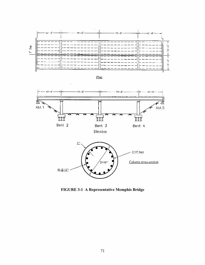
71
FIGURE 3-1 A Representative Memphis Bridge
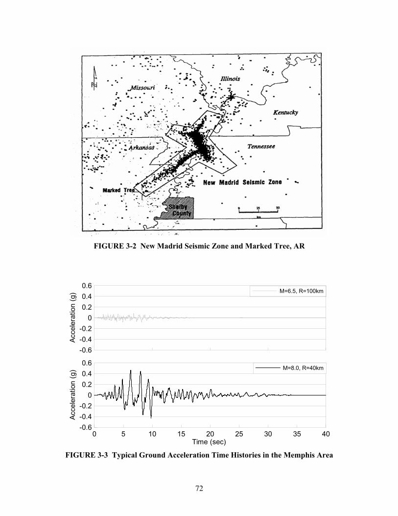
72
FIGURE 3-2 New Madrid Seismic Zone and Marked Tree, AR
0 5 10 15 20 25 30 35 40Time (sec)
-0.6-0.4-0.2
00.20.40.6
Acce
lera
tion
(g) M=8.0, R=40km
-0.6-0.4-0.2
00.20.40.6
Acce
lera
tion
(g) M=6.5, R=100km
FIGURE 3-3 Typical Ground Acceleration Time Histories in the Memphis Area
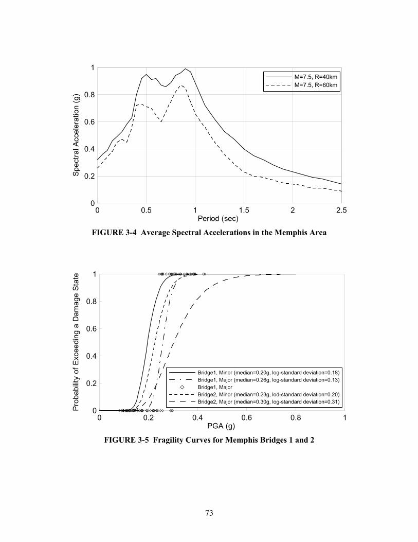
73
0 0.5 1 1.5 2 2.5Period (sec)
0
0.2
0.4
0.6
0.8
1Sp
ectra
l Acc
eler
atio
n (g
)M=7.5, R=40kmM=7.5, R=60km
FIGURE 3-4 Average Spectral Accelerations in the Memphis Area
0 0.2 0.4 0.6 0.8 1PGA (g)
0
0.2
0.4
0.6
0.8
1
Prob
abilit
y of
Exc
eedi
ng a
Dam
age
Stat
e
Bridge1, Minor (median=0.20g, log-standard deviation=0.18)Bridge1, Major (median=0.26g, log-standard deviation=0.13)Bridge1, MajorBridge2, Minor (median=0.23g, lod-standard deviation=0.20)Bridge2, Major (median=0.30g, log-standard deviation=0.31)
FIGURE 3-5 Fragility Curves for Memphis Bridges 1 and 2
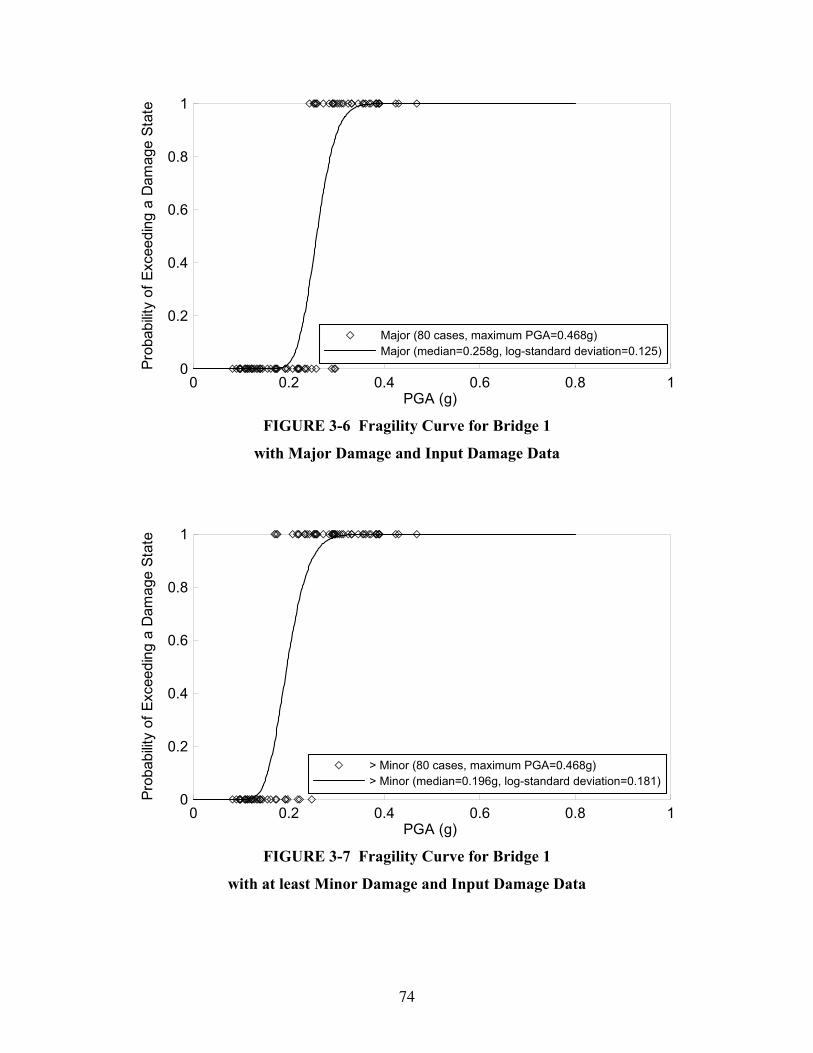
74
0 0.2 0.4 0.6 0.8 1PGA (g)
0
0.2
0.4
0.6
0.8
1
Prob
abilit
y of
Exc
eedi
ng a
Dam
age
Stat
e
Major (80 cases, maximum PGA=0.468g)Major (median=0.258g, log-standard deviation=0.125)
FIGURE 3-6 Fragility Curve for Bridge 1
with Major Damage and Input Damage Data
0
0.2
0.4
0.6
0.8
1
Prob
abilit
y of
Exc
eedi
ng a
Dam
age
Stat
e
0 0.2 0.4 0.6 0.8 1PGA (g)
> Minor (80 cases, maximum PGA=0.468g)> Minor (median=0.196g, log-standard deviation=0.181)
FIGURE 3-7 Fragility Curve for Bridge 1
with at least Minor Damage and Input Damage Data
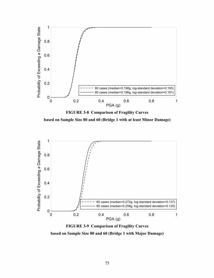
75
0
0.2
0.4
0.6
0.8
1
Prob
abilit
y of
Exc
eedi
ng a
Dam
age
Stat
e
0 0.2 0.4 0.6 0.8 1PGA (g)
60 cases (median=0.198g, log-standard deviation=0.193)80 cases (median=0.196g, log-standard deviation=0.181)
FIGURE 3-8 Comparison of Fragility Curves
based on Sample Size 80 and 60 (Bridge 1 with at least Minor Damage)
0
0.2
0.4
0.6
0.8
1
Prob
abilit
y of
Exc
eedi
ng a
Dam
age
Stat
e
0 0.2 0.4 0.6 0.8 1PGA (g)
60 cases (median=0.272g, log-standard deviation=0.137)80 cases (median=0.258g, log-standard deviation=0.125)
FIGURE 3-9 Comparison of Fragility Curves
based on Sample Size 80 and 60 (Bridge 1 with Major Damage)

77
SECTION 4 MEASURES OF GROUND MOTION ITENSITY
Expressing the fragility curves as a function of other measures of earthquake ground motion
intensity, rather than PGA, has been advocated and promoted by many researchers and
practitioners. The spectral acceleration (SA) is the most prominent among these alternative
measures. Indeed, the spectral acceleration is a good measure under the conditions that the
structural response is primarily in the linear range, structural dynamic characteristics including
damping properties are reasonably well known, geotechnically consistent earthquake ground
motion time histories are either easily specifiable or readily available from pertinent database,
and the state of damage for which the fragility curve is to be developed depends mainly on the
instantaneous maximum inertia force exerted by an episode of the ground motion. However,
when one tries to develop empirical fragility curves on the basis of a large sample of structures,
all different in structural detail if not in geometry, configuration and structural type, subjected to
a severe earthquake, none of these conditions is satisfactorily met, particularly when the damage
state of interest involves, as it usually does, significantly nonlinear structural deformation and/or
the effect of repeated stress or strain cycles. Even for a structure with well-known dynamic
characteristics, the implication of idealizing it as a single-degree-of-freedom system often well
into a nonlinear range is not always palatable. Nevertheless, this study develops fragility curves
for Memphis Bridge 1 as functions of SA. Some researchers also claim that ground velocity-
related quantities are more appropriate for this purpose. They include PGV (peak ground
velocity), SV (spectral velocity) and SI (spectrum intensity). This study also develops fragility
curves as functions of these velocity-related intensity parameters. PGV is the absolute maximum
value of the ground velocity associated with a particular ground velocity time history, SV is the
maximum pseudo (relative) response velocity of a damped single-degree-of-freedom system to
the acceleration time history as a function of natural period, and SI is the average of SV over the
natural period between 0.1 and 2.5 sec following the original Housner’s definition (Housner,
1952). The structural damping coefficient is assumed in all calculations to be 5%, although
Housner used 2% for SI calculations (Housner, 1952).
78
The simulated damage data and the estimated Bridge 1 fragility curves are shown in figures 4-1
and 4-2 as functions of SA respectively for the at least minor and the major state of damage.
Since the simulation is performed primarily under linear analysis when the at least minor damage
(ductility demand > 1.0 for all columns) is considered, figure 4-1 shows the fragility curve
taking in essence the shape of unit step function. This reflects the damage condition primarily
depending on SA and the small effect of the statistical variation associated with structural
materials (fundamental period varies between 1.22 and 1.33 sec) on the damage condition. On
the other hand, the fragility curve for the major damage state (ductility demand > 2.0 for all
columns) rises from zero at SA approximately equal to 0.20g and approaches unity at SA about
equal to 0.45g. Clearly, the shape is no longer close to that of the unit step function, because of
the damage condition that depends on many other factors, mentioned earlier in addition to SA.
Figures 4-3 and 4-4 plot the fragility curves for the same two damage states as functions of PGV.
Since the log-standard deviation represents in approximation the coefficient of variation V of the
lognormal variable, it can be used to measure how sharply the fragility curve rises from zero to
unity. For example, the fragility curves shown in figures 3-7 and 4-3 for the at least minor
damage for Bridge 1 have V = 0.181 and V = 0.207 respectively indicating the fragility curve
developed as a function of PGA has a sharper rise than as a function PGV. On the other hand,
the curves shown in figures 3-6 and 4-4 for the major damage have V = 0.125 as a function of
PGA and V = 0.083 as a function of PGV respectively indicating the opposite trend. These
results suggest that, if a sharper rise of the fragility curve or a smaller log-standard deviation
represents a better measure of the ground motion intensity as a function of which the fragility
curve is developed, PGA is a better measure than PGV in one case but PGV is better for the
other case. Thus, a more elaborate study is needed to resolve this question.
The spectral velocity SV appears to discriminate sharply the occurrence of the state of at least
minor damage as shown in figure 4-5, while such sharpness is not repeated for the state of major
damage as shown in figure 4-6. The reason for this appears to stem from the fact that the
discriminating value of SV in figure 4-5 corresponds to that of SA in figure 4-1 through the
standard tripartite relationship.

79
Finally, fragility curves are developed as functions of spectrum intensity SI as shown in figures
4-7 and 4-8. Four (4) intervals, 0~2.5, 0~3.0, 0~3.5 and 0~4.0 sec, are used over which the
average of SV is taken for the computation of SI. It is of interest to note that the fragility curves
take the shape of the unit step function for the state of major damage as distinctly shown in
figure 4-8, but not for the state of at least minor damage as shown in figure 4-7.
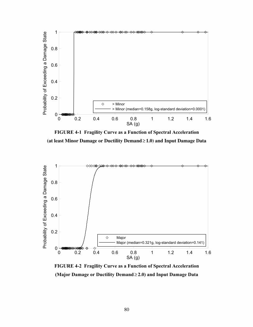
80
0 0.2 0.4 0.6 0.8 1 1.2 1.4 1.6SA (g)
0
0.2
0.4
0.6
0.8
1
Prob
abilit
y of
Exc
eedi
ng a
Dam
age
Stat
e
> Minor> Minor (median=0.158g, log-standard deviation=0.0001)
FIGURE 4-1 Fragility Curve as a Function of Spectral Acceleration
(at least Minor Damage or Ductility Demand ≥ 1.0) and Input Damage Data
0 0.2 0.4 0.6 0.8 1 1.2 1.4 1.6SA (g)
0
0.2
0.4
0.6
0.8
1
Prob
abilit
y of
Exc
eedi
ng a
Dam
age
Stat
e
MajorMajor (median=0.321g, log-standard deviation=0.141)
FIGURE 4-2 Fragility Curve as a Function of Spectral Acceleration
(Major Damage or Ductility Demand ≥ 2.0) and Input Damage Data
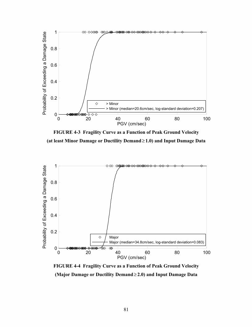
81
0
0.2
0.4
0.6
0.8
1
Prob
abilit
y of
Exc
eedi
ng a
Dam
age
Stat
e
0 20 40 60 80 100PGV (cm/sec)
> Minor> Minor (median=20.6cm/sec, log-standard deviation=0.207)
FIGURE 4-3 Fragility Curve as a Function of Peak Ground Velocity
(at least Minor Damage or Ductility Demand ≥ 1.0) and Input Damage Data
0
0.2
0.4
0.6
0.8
1
Prob
abilit
y of
Exc
eedi
ng a
Dam
age
Stat
e
0 20 40 60 80 100PGV (cm/sec)
MajorMajor (median=34.8cm/sec, log-standard deviation=0.083)
FIGURE 4-4 Fragility Curve as a Function of Peak Ground Velocity
(Major Damage or Ductility Demand ≥ 2.0) and Input Damage Data
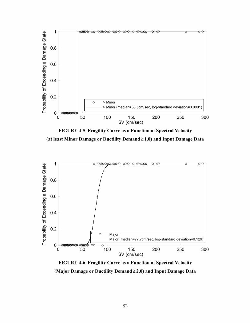
82
0
0.2
0.4
0.6
0.8
1
Prob
abilit
y of
Exc
eedi
ng a
Dam
age
Stat
e
0 50 100 150 200 250 300SV (cm/sec)
> Minor> Minor (median=38.5cm/sec, log-standard deviation=0.0001)
FIGURE 4-5 Fragility Curve as a Function of Spectral Velocity
(at least Minor Damage or Ductility Demand ≥ 1.0) and Input Damage Data
0
0.2
0.4
0.6
0.8
1
Prob
abilit
y of
Exc
eedi
ng a
Dam
age
Stat
e
0 50 100 150 200 250 300SV (cm/sec)
MajorMajor (median=77.7cm/sec, log-standard deviation=0.129)
FIGURE 4-6 Fragility Curve as a Function of Spectral Velocity
(Major Damage or Ductility Demand ≥ 2.0) and Input Damage Data
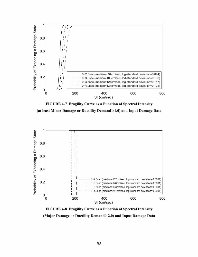
83
0 200 400 600 800SI (cm/sec)
0
0.2
0.4
0.6
0.8
1
Prob
abilit
y of
Exc
eedi
ng a
Dam
age
Stat
e
0~2.5sec (median= 94cm/sec, log-standard deviation=0.094)0~3.0sec (median=109cm/sec, lod-standard deviation=0.108)0~3.5sec (median=121cm/sec, log-standard deviation=0.117)0~4.0sec (median=134cm/sec, log-standard deviation=0.124)
FIGURE 4-7 Fragility Curve as a Function of Spectral Intensity
(at least Minor Damage or Ductility Demand ≥ 1.0) and Input Damage Data
0 200 400 600 800SI (cm/sec)
0
0.2
0.4
0.6
0.8
1
Prob
abilit
y of
Exc
eedi
ng a
Dam
age
Stat
e
0~2.5sec (median=157cm/sec, log-standard deviation=0.0001)0~3.0sec (median=176cm/sec, lod-standard deviation=0.0001)0~3.5sec (median=193cm/sec, log-standard deviation=0.0001)0~4.0sec (median=211cm/sec, log-standard deviation=0.0001)
FIGURE 4-8 Fragility Curve as a Function of Spectral Intensity
(Major Damage or Ductility Demand ≥ 2.0) and Input Damage Data

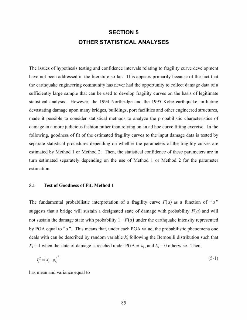
85
SECTION 5 OTHER STATISTICAL ANALYSES
The issues of hypothesis testing and confidence intervals relating to fragility curve development
have not been addressed in the literature so far. This appears primarily because of the fact that
the earthquake engineering community has never had the opportunity to collect damage data of a
sufficiently large sample that can be used to develop fragility curves on the basis of legitimate
statistical analysis. However, the 1994 Northridge and the 1995 Kobe earthquake, inflicting
devastating damage upon many bridges, buildings, port facilities and other engineered structures,
made it possible to consider statistical methods to analyze the probabilistic characteristics of
damage in a more judicious fashion rather than relying on an ad hoc curve fitting exercise. In the
following, goodness of fit of the estimated fragility curves to the input damage data is tested by
separate statistical procedures depending on whether the parameters of the fragility curves are
estimated by Method 1 or Method 2. Then, the statistical confidence of these parameters are in
turn estimated separately depending on the use of Method 1 or Method 2 for the parameter
estimation.
5.1 Test of Goodness of Fit; Method 1
The fundamental probabilistic interpretation of a fragility curve F a( ) as a function of “ a ”
suggests that a bridge will sustain a designated state of damage with probability F a( ) and will
not sustain the damage state with probability 1 − F a( ) under the earthquake intensity represented
by PGA equal to “a ”. This means that, under each PGA value, the probabilistic phenomena one
deals with can be described by random variable Xi following the Bernoulli distribution such that
Xi = 1 when the state of damage is reached under PGA = ai , and Xi = 0 otherwise. Then,
( )22Y X pi i i= − (5-1)
has mean and variance equal to
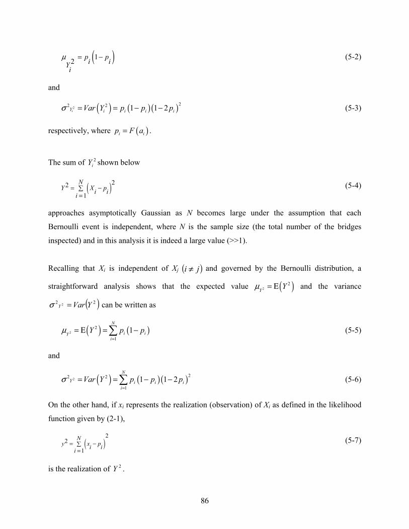
86
( )12 p pi iYi
µ = − (5-2)
and
( ) ( )( )222 2 1 1 2iY i i i iVar Y p p pσ = = − − (5-3)
respectively, where ( )i ip F a= .
The sum of 2iY shown below
( )221
NY X pi ii
= −∑=
(5-4)
approaches asymptotically Gaussian as N becomes large under the assumption that each
Bernoulli event is independent, where N is the sample size (the total number of the bridges
inspected) and in this analysis it is indeed a large value (>>1).
Recalling that Xi is independent of Xj ( )ji ≠ and governed by the Bernoulli distribution, a
straightforward analysis shows that the expected value ( )22
Y Yµ = Ε and the variance
( )22 2 YVarY =σ can be written as
( ) ( )22
11
N
i iYi
Y p pµ=
= Ε = −∑ (5-5)
and
( ) ( )( )222 2
11 1 2
N
Y i i ii
Var Y p p pσ=
= = − −∑ (5-6)
On the other hand, if xi represents the realization (observation) of Xi as defined in the likelihood
function given by (2-1),
( )2
21
Ny x pi ii
= −∑=
(5-7)
is the realization of 2Y .
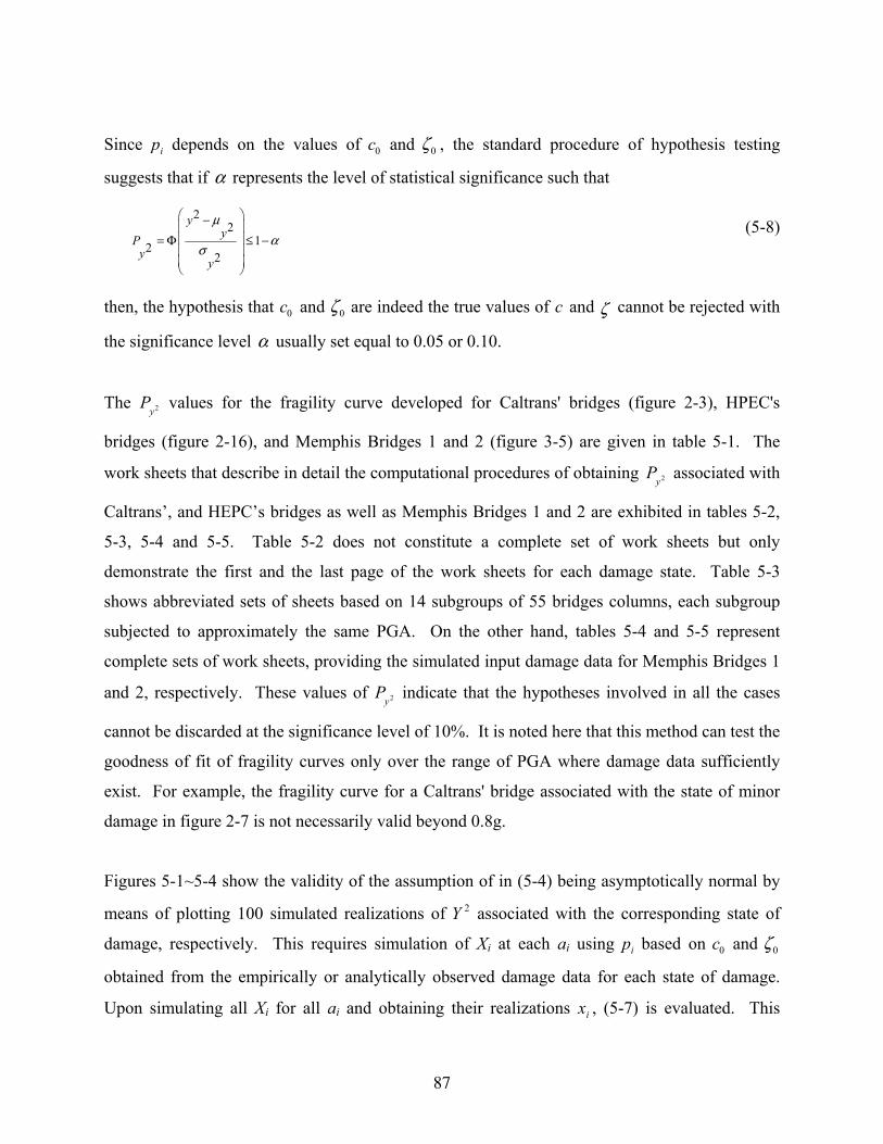
87
Since pi depends on the values of c0 and ζ 0 , the standard procedure of hypothesis testing
suggests that if α represents the level of statistical significance such that
22
122
yyP
yy
µα
σ
− = Φ ≤ −
(5-8)
then, the hypothesis that c0 and ζ 0 are indeed the true values of c and ζ cannot be rejected with
the significance level α usually set equal to 0.05 or 0.10.
The 2yP values for the fragility curve developed for Caltrans' bridges (figure 2-3), HPEC's
bridges (figure 2-16), and Memphis Bridges 1 and 2 (figure 3-5) are given in table 5-1. The
work sheets that describe in detail the computational procedures of obtaining 2yP associated with
Caltrans’, and HEPC’s bridges as well as Memphis Bridges 1 and 2 are exhibited in tables 5-2,
5-3, 5-4 and 5-5. Table 5-2 does not constitute a complete set of work sheets but only
demonstrate the first and the last page of the work sheets for each damage state. Table 5-3
shows abbreviated sets of sheets based on 14 subgroups of 55 bridges columns, each subgroup
subjected to approximately the same PGA. On the other hand, tables 5-4 and 5-5 represent
complete sets of work sheets, providing the simulated input damage data for Memphis Bridges 1
and 2, respectively. These values of 2yP indicate that the hypotheses involved in all the cases
cannot be discarded at the significance level of 10%. It is noted here that this method can test the
goodness of fit of fragility curves only over the range of PGA where damage data sufficiently
exist. For example, the fragility curve for a Caltrans' bridge associated with the state of minor
damage in figure 2-7 is not necessarily valid beyond 0.8g.
Figures 5-1~5-4 show the validity of the assumption of in (5-4) being asymptotically normal by
means of plotting 100 simulated realizations of 2Y associated with the corresponding state of
damage, respectively. This requires simulation of Xi at each ai using pi based on c0 and ζ 0
obtained from the empirically or analytically observed damage data for each state of damage.
Upon simulating all Xi for all ai and obtaining their realizations ix , (5-7) is evaluated. This
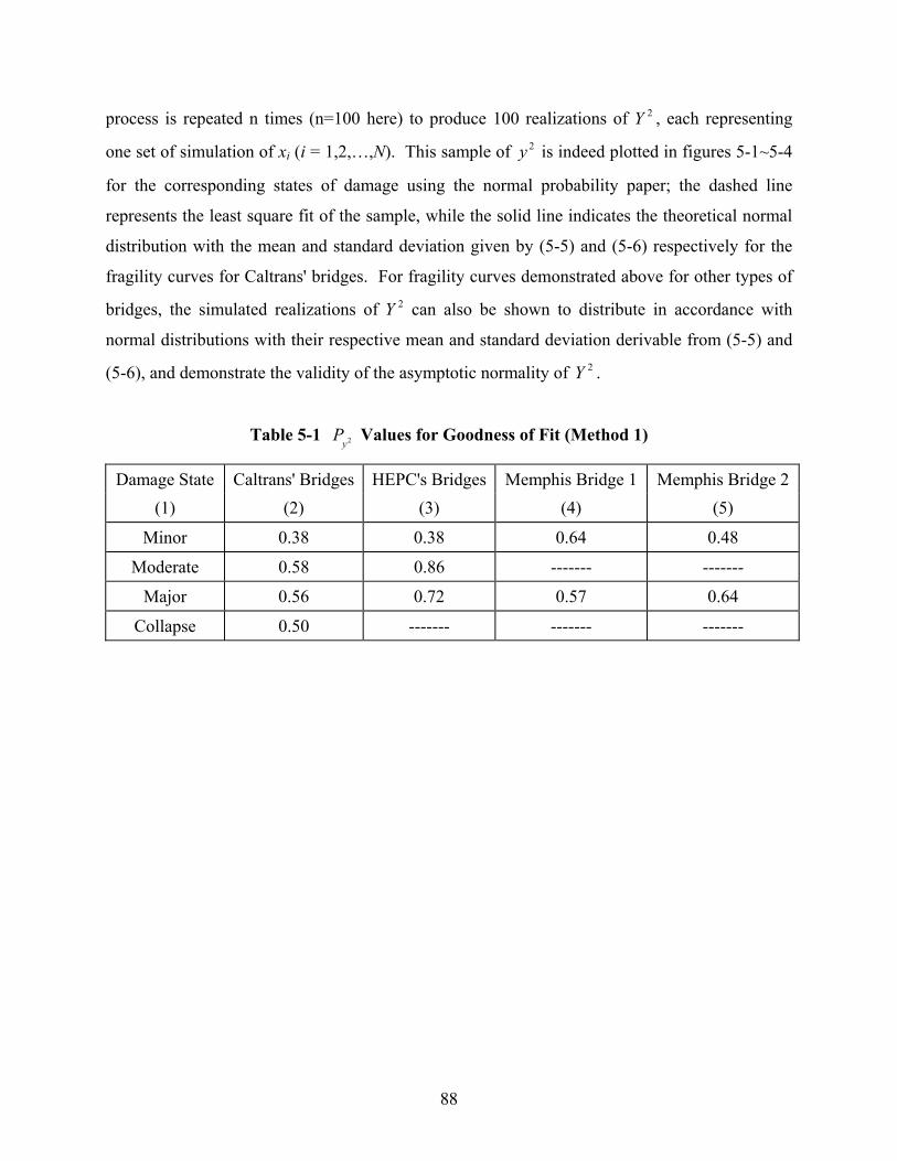
88
process is repeated n times (n=100 here) to produce 100 realizations of 2Y , each representing
one set of simulation of xi (i = 1,2,…,N). This sample of 2y is indeed plotted in figures 5-1~5-4
for the corresponding states of damage using the normal probability paper; the dashed line
represents the least square fit of the sample, while the solid line indicates the theoretical normal
distribution with the mean and standard deviation given by (5-5) and (5-6) respectively for the
fragility curves for Caltrans' bridges. For fragility curves demonstrated above for other types of
bridges, the simulated realizations of 2Y can also be shown to distribute in accordance with
normal distributions with their respective mean and standard deviation derivable from (5-5) and
(5-6), and demonstrate the validity of the asymptotic normality of 2Y .
Table 5-1 2yP Values for Goodness of Fit (Method 1)
Damage State Caltrans' Bridges HEPC's Bridges Memphis Bridge 1 Memphis Bridge 2 (1) (2) (3) (4) (5)
Minor 0.38 0.38 0.64 0.48
Moderate 0.58 0.86 ------- -------
Major 0.56 0.72 0.57 0.64
Collapse 0.50 ------- ------- -------
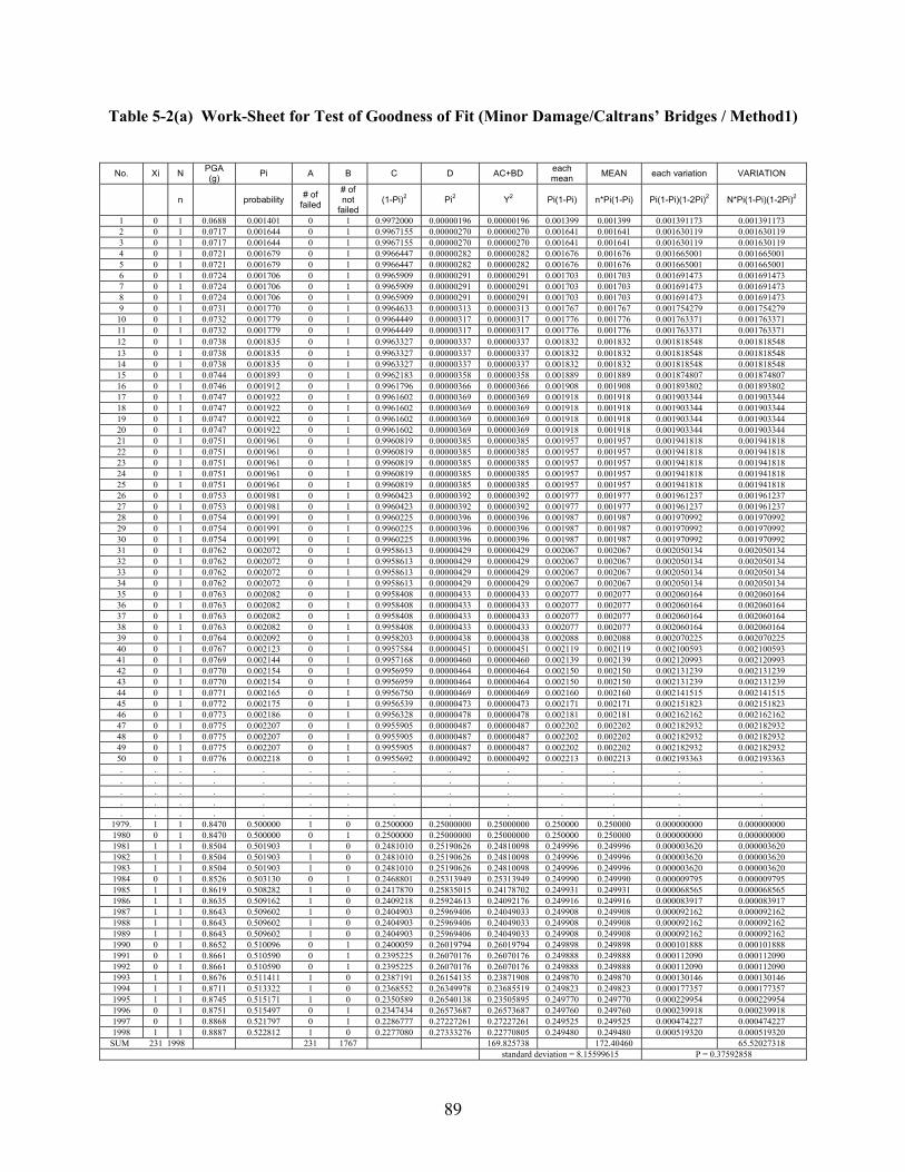
89
Table 5-2(a) Work-Sheet for Test of Goodness of Fit (Minor Damage/Caltrans’ Bridges / Method1)
No. Xi N PGA (g) Pi A B C D AC+BD each
mean MEAN each variation VARIATION
n probability # of failed
# of not
failed (1-Pi)2 Pi2 Y2 Pi(1-Pi) n*Pi(1-Pi) Pi(1-Pi)(1-2Pi)2 N*Pi(1-Pi)(1-2Pi)2
1 0 1 0.0688 0.001401 0 1 0.9972000 0.00000196 0.00000196 0.001399 0.001399 0.001391173 0.001391173 2 0 1 0.0717 0.001644 0 1 0.9967155 0.00000270 0.00000270 0.001641 0.001641 0.001630119 0.001630119 3 0 1 0.0717 0.001644 0 1 0.9967155 0.00000270 0.00000270 0.001641 0.001641 0.001630119 0.001630119 4 0 1 0.0721 0.001679 0 1 0.9966447 0.00000282 0.00000282 0.001676 0.001676 0.001665001 0.001665001 5 0 1 0.0721 0.001679 0 1 0.9966447 0.00000282 0.00000282 0.001676 0.001676 0.001665001 0.001665001 6 0 1 0.0724 0.001706 0 1 0.9965909 0.00000291 0.00000291 0.001703 0.001703 0.001691473 0.001691473 7 0 1 0.0724 0.001706 0 1 0.9965909 0.00000291 0.00000291 0.001703 0.001703 0.001691473 0.001691473 8 0 1 0.0724 0.001706 0 1 0.9965909 0.00000291 0.00000291 0.001703 0.001703 0.001691473 0.001691473 9 0 1 0.0731 0.001770 0 1 0.9964633 0.00000313 0.00000313 0.001767 0.001767 0.001754279 0.001754279 10 0 1 0.0732 0.001779 0 1 0.9964449 0.00000317 0.00000317 0.001776 0.001776 0.001763371 0.001763371 11 0 1 0.0732 0.001779 0 1 0.9964449 0.00000317 0.00000317 0.001776 0.001776 0.001763371 0.001763371 12 0 1 0.0738 0.001835 0 1 0.9963327 0.00000337 0.00000337 0.001832 0.001832 0.001818548 0.001818548 13 0 1 0.0738 0.001835 0 1 0.9963327 0.00000337 0.00000337 0.001832 0.001832 0.001818548 0.001818548 14 0 1 0.0738 0.001835 0 1 0.9963327 0.00000337 0.00000337 0.001832 0.001832 0.001818548 0.001818548 15 0 1 0.0744 0.001893 0 1 0.9962183 0.00000358 0.00000358 0.001889 0.001889 0.001874807 0.001874807 16 0 1 0.0746 0.001912 0 1 0.9961796 0.00000366 0.00000366 0.001908 0.001908 0.001893802 0.001893802 17 0 1 0.0747 0.001922 0 1 0.9961602 0.00000369 0.00000369 0.001918 0.001918 0.001903344 0.001903344 18 0 1 0.0747 0.001922 0 1 0.9961602 0.00000369 0.00000369 0.001918 0.001918 0.001903344 0.001903344 19 0 1 0.0747 0.001922 0 1 0.9961602 0.00000369 0.00000369 0.001918 0.001918 0.001903344 0.001903344 20 0 1 0.0747 0.001922 0 1 0.9961602 0.00000369 0.00000369 0.001918 0.001918 0.001903344 0.001903344 21 0 1 0.0751 0.001961 0 1 0.9960819 0.00000385 0.00000385 0.001957 0.001957 0.001941818 0.001941818 22 0 1 0.0751 0.001961 0 1 0.9960819 0.00000385 0.00000385 0.001957 0.001957 0.001941818 0.001941818 23 0 1 0.0751 0.001961 0 1 0.9960819 0.00000385 0.00000385 0.001957 0.001957 0.001941818 0.001941818 24 0 1 0.0751 0.001961 0 1 0.9960819 0.00000385 0.00000385 0.001957 0.001957 0.001941818 0.001941818 25 0 1 0.0751 0.001961 0 1 0.9960819 0.00000385 0.00000385 0.001957 0.001957 0.001941818 0.001941818 26 0 1 0.0753 0.001981 0 1 0.9960423 0.00000392 0.00000392 0.001977 0.001977 0.001961237 0.001961237 27 0 1 0.0753 0.001981 0 1 0.9960423 0.00000392 0.00000392 0.001977 0.001977 0.001961237 0.001961237 28 0 1 0.0754 0.001991 0 1 0.9960225 0.00000396 0.00000396 0.001987 0.001987 0.001970992 0.001970992 29 0 1 0.0754 0.001991 0 1 0.9960225 0.00000396 0.00000396 0.001987 0.001987 0.001970992 0.001970992 30 0 1 0.0754 0.001991 0 1 0.9960225 0.00000396 0.00000396 0.001987 0.001987 0.001970992 0.001970992 31 0 1 0.0762 0.002072 0 1 0.9958613 0.00000429 0.00000429 0.002067 0.002067 0.002050134 0.002050134 32 0 1 0.0762 0.002072 0 1 0.9958613 0.00000429 0.00000429 0.002067 0.002067 0.002050134 0.002050134 33 0 1 0.0762 0.002072 0 1 0.9958613 0.00000429 0.00000429 0.002067 0.002067 0.002050134 0.002050134 34 0 1 0.0762 0.002072 0 1 0.9958613 0.00000429 0.00000429 0.002067 0.002067 0.002050134 0.002050134 35 0 1 0.0763 0.002082 0 1 0.9958408 0.00000433 0.00000433 0.002077 0.002077 0.002060164 0.002060164 36 0 1 0.0763 0.002082 0 1 0.9958408 0.00000433 0.00000433 0.002077 0.002077 0.002060164 0.002060164 37 0 1 0.0763 0.002082 0 1 0.9958408 0.00000433 0.00000433 0.002077 0.002077 0.002060164 0.002060164 38 0 1 0.0763 0.002082 0 1 0.9958408 0.00000433 0.00000433 0.002077 0.002077 0.002060164 0.002060164 39 0 1 0.0764 0.002092 0 1 0.9958203 0.00000438 0.00000438 0.002088 0.002088 0.002070225 0.002070225 40 0 1 0.0767 0.002123 0 1 0.9957584 0.00000451 0.00000451 0.002119 0.002119 0.002100593 0.002100593 41 0 1 0.0769 0.002144 0 1 0.9957168 0.00000460 0.00000460 0.002139 0.002139 0.002120993 0.002120993 42 0 1 0.0770 0.002154 0 1 0.9956959 0.00000464 0.00000464 0.002150 0.002150 0.002131239 0.002131239 43 0 1 0.0770 0.002154 0 1 0.9956959 0.00000464 0.00000464 0.002150 0.002150 0.002131239 0.002131239 44 0 1 0.0771 0.002165 0 1 0.9956750 0.00000469 0.00000469 0.002160 0.002160 0.002141515 0.002141515 45 0 1 0.0772 0.002175 0 1 0.9956539 0.00000473 0.00000473 0.002171 0.002171 0.002151823 0.002151823 46 0 1 0.0773 0.002186 0 1 0.9956328 0.00000478 0.00000478 0.002181 0.002181 0.002162162 0.002162162 47 0 1 0.0775 0.002207 0 1 0.9955905 0.00000487 0.00000487 0.002202 0.002202 0.002182932 0.002182932 48 0 1 0.0775 0.002207 0 1 0.9955905 0.00000487 0.00000487 0.002202 0.002202 0.002182932 0.002182932 49 0 1 0.0775 0.002207 0 1 0.9955905 0.00000487 0.00000487 0.002202 0.002202 0.002182932 0.002182932 50 0 1 0.0776 0.002218 0 1 0.9955692 0.00000492 0.00000492 0.002213 0.002213 0.002193363 0.002193363 . . . . . . . . . . . . . . . . . . . . . . . . . . . . . . . . . . . . . . . . . . . . . . . . . . . . . . . . . . . . . . . . . . . . . .
1979. 1 1 0.8470 0.500000 1 0 0.2500000 0.25000000 0.25000000 0.250000 0.250000 0.000000000 0.000000000 1980 0 1 0.8470 0.500000 0 1 0.2500000 0.25000000 0.25000000 0.250000 0.250000 0.000000000 0.000000000 1981 1 1 0.8504 0.501903 1 0 0.2481010 0.25190626 0.24810098 0.249996 0.249996 0.000003620 0.000003620 1982 1 1 0.8504 0.501903 1 0 0.2481010 0.25190626 0.24810098 0.249996 0.249996 0.000003620 0.000003620 1983 1 1 0.8504 0.501903 1 0 0.2481010 0.25190626 0.24810098 0.249996 0.249996 0.000003620 0.000003620 1984 0 1 0.8526 0.503130 0 1 0.2468801 0.25313949 0.25313949 0.249990 0.249990 0.000009795 0.000009795 1985 1 1 0.8619 0.508282 1 0 0.2417870 0.25835015 0.24178702 0.249931 0.249931 0.000068565 0.000068565 1986 1 1 0.8635 0.509162 1 0 0.2409218 0.25924613 0.24092176 0.249916 0.249916 0.000083917 0.000083917 1987 1 1 0.8643 0.509602 1 0 0.2404903 0.25969406 0.24049033 0.249908 0.249908 0.000092162 0.000092162 1988 1 1 0.8643 0.509602 1 0 0.2404903 0.25969406 0.24049033 0.249908 0.249908 0.000092162 0.000092162 1989 1 1 0.8643 0.509602 1 0 0.2404903 0.25969406 0.24049033 0.249908 0.249908 0.000092162 0.000092162 1990 0 1 0.8652 0.510096 0 1 0.2400059 0.26019794 0.26019794 0.249898 0.249898 0.000101888 0.000101888 1991 0 1 0.8661 0.510590 0 1 0.2395225 0.26070176 0.26070176 0.249888 0.249888 0.000112090 0.000112090 1992 0 1 0.8661 0.510590 0 1 0.2395225 0.26070176 0.26070176 0.249888 0.249888 0.000112090 0.000112090 1993 1 1 0.8676 0.511411 1 0 0.2387191 0.26154135 0.23871908 0.249870 0.249870 0.000130146 0.000130146 1994 1 1 0.8711 0.513322 1 0 0.2368552 0.26349978 0.23685519 0.249823 0.249823 0.000177357 0.000177357 1995 1 1 0.8745 0.515171 1 0 0.2350589 0.26540138 0.23505895 0.249770 0.249770 0.000229954 0.000229954 1996 0 1 0.8751 0.515497 0 1 0.2347434 0.26573687 0.26573687 0.249760 0.249760 0.000239918 0.000239918 1997 0 1 0.8868 0.521797 0 1 0.2286777 0.27227261 0.27227261 0.249525 0.249525 0.000474227 0.000474227 1998 1 1 0.8887 0.522812 1 0 0.2277080 0.27333276 0.22770805 0.249480 0.249480 0.000519320 0.000519320
SUM 231 1998 231 1767 169.825738 172.40460 65.52027318 standard deviation = 8.15599615 P = 0.37592858
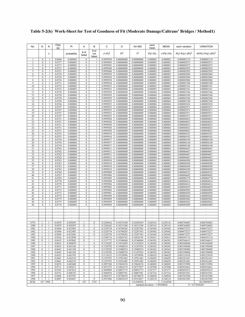
90
Table 5-2(b) Work-Sheet for Test of Goodness of Fit (Moderate Damage/Caltrans’ Bridges / Method1)
No. Xi N PGA (g) Pi A B C D AC+BD each
mean MEAN each variation VARIATION
n probability # of failed
# of not
failed (1-Pi)2 Pi2 Y2 Pi(1-Pi) n*Pi(1-Pi) Pi(1-Pi)(1-2Pi)2 N*Pi(1-Pi)(1-2Pi)2
1 0 1 0.0688 0.000002 0 1 0.9999958 0.00000000 0.00000000 0.000002 0.000002 0.000002119 0.000002119 2 0 1 0.0717 0.000003 0 1 0.9999943 0.00000000 0.00000000 0.000003 0.000003 0.000002873 0.000002873 3 0 1 0.0717 0.000003 0 1 0.9999943 0.00000000 0.00000000 0.000003 0.000003 0.000002873 0.000002873 4 0 1 0.0721 0.000003 0 1 0.9999940 0.00000000 0.00000000 0.000003 0.000003 0.000002992 0.000002992 5 0 1 0.0721 0.000003 0 1 0.9999940 0.00000000 0.00000000 0.000003 0.000003 0.000002992 0.000002992 6 0 1 0.0724 0.000003 0 1 0.9999938 0.00000000 0.00000000 0.000003 0.000003 0.000003084 0.000003084 7 0 1 0.0724 0.000003 0 1 0.9999938 0.00000000 0.00000000 0.000003 0.000003 0.000003084 0.000003084 8 0 1 0.0724 0.000003 0 1 0.9999938 0.00000000 0.00000000 0.000003 0.000003 0.000003084 0.000003084 9 0 1 0.0731 0.000003 0 1 0.9999934 0.00000000 0.00000000 0.000003 0.000003 0.000003308 0.000003308 10 0 1 0.0732 0.000003 0 1 0.9999933 0.00000000 0.00000000 0.000003 0.000003 0.000003341 0.000003341 11 0 1 0.0732 0.000003 0 1 0.9999933 0.00000000 0.00000000 0.000003 0.000003 0.000003341 0.000003341 12 0 1 0.0738 0.000004 0 1 0.9999929 0.00000000 0.00000000 0.000004 0.000004 0.000003546 0.000003546 13 0 1 0.0738 0.000004 0 1 0.9999929 0.00000000 0.00000000 0.000004 0.000004 0.000003546 0.000003546 14 0 1 0.0738 0.000004 0 1 0.9999929 0.00000000 0.00000000 0.000004 0.000004 0.000003546 0.000003546 15 0 1 0.0744 0.000004 0 1 0.9999925 0.00000000 0.00000000 0.000004 0.000004 0.000003760 0.000003760 16 0 1 0.0746 0.000004 0 1 0.9999923 0.00000000 0.00000000 0.000004 0.000004 0.000003834 0.000003834 17 0 1 0.0747 0.000004 0 1 0.9999923 0.00000000 0.00000000 0.000004 0.000004 0.000003871 0.000003871 18 0 1 0.0747 0.000004 0 1 0.9999923 0.00000000 0.00000000 0.000004 0.000004 0.000003871 0.000003871 19 0 1 0.0747 0.000004 0 1 0.9999923 0.00000000 0.00000000 0.000004 0.000004 0.000003871 0.000003871 20 0 1 0.0747 0.000004 0 1 0.9999923 0.00000000 0.00000000 0.000004 0.000004 0.000003871 0.000003871 21 0 1 0.0751 0.000004 0 1 0.9999920 0.00000000 0.00000000 0.000004 0.000004 0.000004023 0.000004023 22 0 1 0.0751 0.000004 0 1 0.9999920 0.00000000 0.00000000 0.000004 0.000004 0.000004023 0.000004023 23 0 1 0.0751 0.000004 0 1 0.9999920 0.00000000 0.00000000 0.000004 0.000004 0.000004023 0.000004023 24 0 1 0.0751 0.000004 0 1 0.9999920 0.00000000 0.00000000 0.000004 0.000004 0.000004023 0.000004023 25 0 1 0.0751 0.000004 0 1 0.9999920 0.00000000 0.00000000 0.000004 0.000004 0.000004023 0.000004023 26 0 1 0.0753 0.000004 0 1 0.9999918 0.00000000 0.00000000 0.000004 0.000004 0.000004101 0.000004101 27 0 1 0.0753 0.000004 0 1 0.9999918 0.00000000 0.00000000 0.000004 0.000004 0.000004101 0.000004101 28 0 1 0.0754 0.000004 0 1 0.9999917 0.00000000 0.00000000 0.000004 0.000004 0.000004140 0.000004140 29 0 1 0.0754 0.000004 0 1 0.9999917 0.00000000 0.00000000 0.000004 0.000004 0.000004140 0.000004140 30 0 1 0.0754 0.000004 0 1 0.9999917 0.00000000 0.00000000 0.000004 0.000004 0.000004140 0.000004140 31 0 1 0.0762 0.000004 0 1 0.9999911 0.00000000 0.00000000 0.000004 0.000004 0.000004467 0.000004467 32 0 1 0.0762 0.000004 0 1 0.9999911 0.00000000 0.00000000 0.000004 0.000004 0.000004467 0.000004467 33 0 1 0.0762 0.000004 0 1 0.9999911 0.00000000 0.00000000 0.000004 0.000004 0.000004467 0.000004467 34 0 1 0.0762 0.000004 0 1 0.9999911 0.00000000 0.00000000 0.000004 0.000004 0.000004467 0.000004467 35 0 1 0.0763 0.000005 0 1 0.9999910 0.00000000 0.00000000 0.000005 0.000005 0.000004509 0.000004509 36 0 1 0.0763 0.000005 0 1 0.9999910 0.00000000 0.00000000 0.000005 0.000005 0.000004509 0.000004509 37 0 1 0.0763 0.000005 0 1 0.9999910 0.00000000 0.00000000 0.000005 0.000005 0.000004509 0.000004509 38 0 1 0.0763 0.000005 0 1 0.9999910 0.00000000 0.00000000 0.000005 0.000005 0.000004509 0.000004509 39 0 1 0.0764 0.000005 0 1 0.9999909 0.00000000 0.00000000 0.000005 0.000005 0.000004552 0.000004552 40 0 1 0.0767 0.000005 0 1 0.9999906 0.00000000 0.00000000 0.000005 0.000005 0.000004682 0.000004682 41 0 1 0.0769 0.000005 0 1 0.9999905 0.00000000 0.00000000 0.000005 0.000005 0.000004770 0.000004770 42 0 1 0.0770 0.000005 0 1 0.9999904 0.00000000 0.00000000 0.000005 0.000005 0.000004814 0.000004814 43 0 1 0.0770 0.000005 0 1 0.9999904 0.00000000 0.00000000 0.000005 0.000005 0.000004814 0.000004814 44 0 1 0.0771 0.000005 0 1 0.9999903 0.00000000 0.00000000 0.000005 0.000005 0.000004859 0.000004859 45 0 1 0.0772 0.000005 0 1 0.9999902 0.00000000 0.00000000 0.000005 0.000005 0.000004905 0.000004905 46 0 1 0.0773 0.000005 0 1 0.9999901 0.00000000 0.00000000 0.000005 0.000005 0.000004950 0.000004950 47 0 1 0.0775 0.000005 0 1 0.9999899 0.00000000 0.00000000 0.000005 0.000005 0.000005042 0.000005042 48 0 1 0.0775 0.000005 0 1 0.9999899 0.00000000 0.00000000 0.000005 0.000005 0.000005042 0.000005042 49 0 1 0.0775 0.000005 0 1 0.9999899 0.00000000 0.00000000 0.000005 0.000005 0.000005042 0.000005042 50 0 1 0.0776 0.000005 0 1 0.9999898 0.00000000 0.00000000 0.000005 0.000005 0.000005089 0.000005089 . . . . . . . . . . . . . . . . . . . . . . . . . . . . . . . . . . . . . . . . . . . . . . . . . . . . . . . . . . . . . . . . . . . . . .
1979. 1 1 0.8470 0.430295 1 0 0.3245642 0.18515348 0.32456419 0.245141 0.245141 0.004764403 0.004764403 1980 0 1 0.8470 0.430295 0 1 0.3245642 0.18515348 0.18515348 0.245141 0.245141 0.004764403 0.004764403 1981 1 1 0.8504 0.432485 1 0 0.3220738 0.18704285 0.32207383 0.245442 0.245442 0.004475227 0.004475227 1982 1 1 0.8504 0.432485 1 0 0.3220738 0.18704285 0.32207383 0.245442 0.245442 0.004475227 0.004475227 1983 1 1 0.8504 0.432485 1 0 0.3220738 0.18704285 0.32207383 0.245442 0.245442 0.004475227 0.004475227 1984 0 1 0.8526 0.433898 0 1 0.3204716 0.18826742 0.18826742 0.245631 0.245631 0.004293114 0.004293114 1985 0 1 0.8619 0.439842 0 1 0.3137772 0.19346084 0.19346084 0.246381 0.246381 0.003566615 0.003566615 1986 1 1 0.8635 0.440859 1 0 0.3126382 0.19435699 0.31263824 0.246502 0.246502 0.003448680 0.003448680 1987 1 1 0.8643 0.441368 1 0 0.3120702 0.19480534 0.31207018 0.246562 0.246562 0.003390488 0.003390488 1988 0 1 0.8643 0.441368 0 1 0.3120702 0.19480534 0.19480534 0.246562 0.246562 0.003390488 0.003390488 1989 1 1 0.8643 0.441368 1 0 0.3120702 0.19480534 0.31207018 0.246562 0.246562 0.003390488 0.003390488 1990 0 1 0.8652 0.441939 0 1 0.3114322 0.19530996 0.19530996 0.246629 0.246629 0.003325638 0.003325638 1991 0 1 0.8661 0.442510 0 1 0.3107955 0.19581482 0.19581482 0.246695 0.246695 0.003261441 0.003261441 1992 0 1 0.8661 0.442510 0 1 0.3107955 0.19581482 0.19581482 0.246695 0.246695 0.003261441 0.003261441 1993 0 1 0.8676 0.443460 0 1 0.3097368 0.19665676 0.19665676 0.246803 0.246803 0.003155896 0.003155896 1994 1 1 0.8711 0.445672 1 0 0.3072793 0.19862374 0.30727927 0.247048 0.247048 0.002916661 0.002916661 1995 0 1 0.8745 0.447814 0 1 0.3049089 0.20053773 0.20053773 0.247277 0.247277 0.002693672 0.002693672 1996 0 1 0.8751 0.448192 0 1 0.3044924 0.20087581 0.20087581 0.247316 0.247316 0.002655281 0.002655281 1997 0 1 0.8868 0.455507 0 1 0.2964725 0.20748670 0.20748670 0.248020 0.248020 0.001963944 0.001963944 1998 1 1 0.8887 0.456687 1 0 0.2951886 0.20856339 0.29518857 0.248124 0.248124 0.001861903 0.001861903
SUM 147 1998 147 1767 116.046926 114.64548 50.350948977 standard deviation = 7.09584026 P = 0.57828269
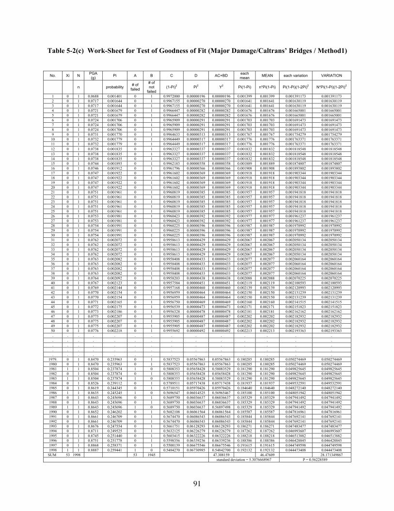
91
Table 5-2(c) Work-Sheet for Test of Goodness of Fit (Major Damage/Caltrans’ Bridges / Method1)
No. Xi N PGA (g) Pi A B C D AC+BD each
mean MEAN each variation VARIATION
n probability # of failed
# of not
failed (1-Pi)2 Pi2 Y2 Pi(1-Pi) n*Pi(1-Pi) Pi(1-Pi)(1-2Pi)2 N*Pi(1-Pi)(1-2Pi)2
1 0 1 0.0688 0.001401 0 1 0.9972000 0.00000196 0.00000196 0.001399 0.001399 0.001391173 0.001391173 2 0 1 0.0717 0.001644 0 1 0.9967155 0.00000270 0.00000270 0.001641 0.001641 0.001630119 0.001630119 3 0 1 0.0717 0.001644 0 1 0.9967155 0.00000270 0.00000270 0.001641 0.001641 0.001630119 0.001630119 4 0 1 0.0721 0.001679 0 1 0.9966447 0.00000282 0.00000282 0.001676 0.001676 0.001665001 0.001665001 5 0 1 0.0721 0.001679 0 1 0.9966447 0.00000282 0.00000282 0.001676 0.001676 0.001665001 0.001665001 6 0 1 0.0724 0.001706 0 1 0.9965909 0.00000291 0.00000291 0.001703 0.001703 0.001691473 0.001691473 7 0 1 0.0724 0.001706 0 1 0.9965909 0.00000291 0.00000291 0.001703 0.001703 0.001691473 0.001691473 8 0 1 0.0724 0.001706 0 1 0.9965909 0.00000291 0.00000291 0.001703 0.001703 0.001691473 0.001691473 9 0 1 0.0731 0.001770 0 1 0.9964633 0.00000313 0.00000313 0.001767 0.001767 0.001754279 0.001754279 10 0 1 0.0732 0.001779 0 1 0.9964449 0.00000317 0.00000317 0.001776 0.001776 0.001763371 0.001763371 11 0 1 0.0732 0.001779 0 1 0.9964449 0.00000317 0.00000317 0.001776 0.001776 0.001763371 0.001763371 12 0 1 0.0738 0.001835 0 1 0.9963327 0.00000337 0.00000337 0.001832 0.001832 0.001818548 0.001818548 13 0 1 0.0738 0.001835 0 1 0.9963327 0.00000337 0.00000337 0.001832 0.001832 0.001818548 0.001818548 14 0 1 0.0738 0.001835 0 1 0.9963327 0.00000337 0.00000337 0.001832 0.001832 0.001818548 0.001818548 15 0 1 0.0744 0.001893 0 1 0.9962183 0.00000358 0.00000358 0.001889 0.001889 0.001874807 0.001874807 16 0 1 0.0746 0.001912 0 1 0.9961796 0.00000366 0.00000366 0.001908 0.001908 0.001893802 0.001893802 17 0 1 0.0747 0.001922 0 1 0.9961602 0.00000369 0.00000369 0.001918 0.001918 0.001903344 0.001903344 18 0 1 0.0747 0.001922 0 1 0.9961602 0.00000369 0.00000369 0.001918 0.001918 0.001903344 0.001903344 19 0 1 0.0747 0.001922 0 1 0.9961602 0.00000369 0.00000369 0.001918 0.001918 0.001903344 0.001903344 20 0 1 0.0747 0.001922 0 1 0.9961602 0.00000369 0.00000369 0.001918 0.001918 0.001903344 0.001903344 21 0 1 0.0751 0.001961 0 1 0.9960819 0.00000385 0.00000385 0.001957 0.001957 0.001941818 0.001941818 22 0 1 0.0751 0.001961 0 1 0.9960819 0.00000385 0.00000385 0.001957 0.001957 0.001941818 0.001941818 23 0 1 0.0751 0.001961 0 1 0.9960819 0.00000385 0.00000385 0.001957 0.001957 0.001941818 0.001941818 24 0 1 0.0751 0.001961 0 1 0.9960819 0.00000385 0.00000385 0.001957 0.001957 0.001941818 0.001941818 25 0 1 0.0751 0.001961 0 1 0.9960819 0.00000385 0.00000385 0.001957 0.001957 0.001941818 0.001941818 26 0 1 0.0753 0.001981 0 1 0.9960423 0.00000392 0.00000392 0.001977 0.001977 0.001961237 0.001961237 27 0 1 0.0753 0.001981 0 1 0.9960423 0.00000392 0.00000392 0.001977 0.001977 0.001961237 0.001961237 28 0 1 0.0754 0.001991 0 1 0.9960225 0.00000396 0.00000396 0.001987 0.001987 0.001970992 0.001970992 29 0 1 0.0754 0.001991 0 1 0.9960225 0.00000396 0.00000396 0.001987 0.001987 0.001970992 0.001970992 30 0 1 0.0754 0.001991 0 1 0.9960225 0.00000396 0.00000396 0.001987 0.001987 0.001970992 0.001970992 31 0 1 0.0762 0.002072 0 1 0.9958613 0.00000429 0.00000429 0.002067 0.002067 0.002050134 0.002050134 32 0 1 0.0762 0.002072 0 1 0.9958613 0.00000429 0.00000429 0.002067 0.002067 0.002050134 0.002050134 33 0 1 0.0762 0.002072 0 1 0.9958613 0.00000429 0.00000429 0.002067 0.002067 0.002050134 0.002050134 34 0 1 0.0762 0.002072 0 1 0.9958613 0.00000429 0.00000429 0.002067 0.002067 0.002050134 0.002050134 35 0 1 0.0763 0.002082 0 1 0.9958408 0.00000433 0.00000433 0.002077 0.002077 0.002060164 0.002060164 36 0 1 0.0763 0.002082 0 1 0.9958408 0.00000433 0.00000433 0.002077 0.002077 0.002060164 0.002060164 37 0 1 0.0763 0.002082 0 1 0.9958408 0.00000433 0.00000433 0.002077 0.002077 0.002060164 0.002060164 38 0 1 0.0763 0.002082 0 1 0.9958408 0.00000433 0.00000433 0.002077 0.002077 0.002060164 0.002060164 39 0 1 0.0764 0.002092 0 1 0.9958203 0.00000438 0.00000438 0.002088 0.002088 0.002070225 0.002070225 40 0 1 0.0767 0.002123 0 1 0.9957584 0.00000451 0.00000451 0.002119 0.002119 0.002100593 0.002100593 41 0 1 0.0769 0.002144 0 1 0.9957168 0.00000460 0.00000460 0.002139 0.002139 0.002120993 0.002120993 42 0 1 0.0770 0.002154 0 1 0.9956959 0.00000464 0.00000464 0.002150 0.002150 0.002131239 0.002131239 43 0 1 0.0770 0.002154 0 1 0.9956959 0.00000464 0.00000464 0.002150 0.002150 0.002131239 0.002131239 44 0 1 0.0771 0.002165 0 1 0.9956750 0.00000469 0.00000469 0.002160 0.002160 0.002141515 0.002141515 45 0 1 0.0772 0.002175 0 1 0.9956539 0.00000473 0.00000473 0.002171 0.002171 0.002151823 0.002151823 46 0 1 0.0773 0.002186 0 1 0.9956328 0.00000478 0.00000478 0.002181 0.002181 0.002162162 0.002162162 47 0 1 0.0775 0.002207 0 1 0.9955905 0.00000487 0.00000487 0.002202 0.002202 0.002182932 0.002182932 48 0 1 0.0775 0.002207 0 1 0.9955905 0.00000487 0.00000487 0.002202 0.002202 0.002182932 0.002182932 49 0 1 0.0775 0.002207 0 1 0.9955905 0.00000487 0.00000487 0.002202 0.002202 0.002182932 0.002182932 50 0 1 0.0776 0.002218 0 1 0.9955692 0.00000492 0.00000492 0.002213 0.002213 0.002193363 0.002193363 . . . . . . . . . . . . . . . . . . . . . . . . . . . . . . . . . . . . . . . . . . . . . . . . . . . . . . . . . . . . . . . . . . . . . .
1979. 0 1 0.8470 0.235963 0 1 0.5837523 0.05567863 0.05567863 0.180285 0.180285 0.050274469 0.050274469 1980 0 1 0.8470 0.235963 0 1 0.5837523 0.05567863 0.05567863 0.180285 0.180285 0.050274469 0.050274469 1981 1 1 0.8504 0.237874 1 0 0.5808353 0.05658428 0.58083529 0.181290 0.181290 0.049825645 0.049825645 1982 0 1 0.8504 0.237874 0 1 0.5808353 0.05658428 0.05658428 0.181290 0.181290 0.049825645 0.049825645 1983 1 1 0.8504 0.237874 1 0 0.5808353 0.05658428 0.58083529 0.181290 0.181290 0.049825645 0.049825645 1984 0 1 0.8526 0.239112 0 1 0.5789511 0.05717438 0.05717438 0.181937 0.181937 0.049532591 0.049532591 1985 0 1 0.8619 0.244345 0 1 0.5710151 0.05970426 0.05970426 0.184640 0.184640 0.048272140 0.048272140 1986 1 1 0.8635 0.245245 1 0 0.5696547 0.06014525 0.56965467 0.185100 0.185100 0.048051942 0.048051942 1987 0 1 0.8643 0.245696 0 1 0.5689750 0.06036637 0.06036637 0.185329 0.185329 0.047941492 0.047941492 1988 0 1 0.8643 0.245696 0 1 0.5689750 0.06036637 0.06036637 0.185329 0.185329 0.047941492 0.047941492 1989 1 1 0.8643 0.245696 1 0 0.5689750 0.06036637 0.56897498 0.185329 0.185329 0.047941492 0.047941492 1990 0 1 0.8652 0.246202 0 1 0.5682108 0.06061564 0.06061564 0.185587 0.185587 0.047816961 0.047816961 1991 0 1 0.8661 0.246709 0 1 0.5674470 0.06086543 0.06086543 0.185844 0.185844 0.047692141 0.047692141 1992 0 1 0.8661 0.246709 0 1 0.5674470 0.06086543 0.06086543 0.185844 0.185844 0.047692141 0.047692141 1993 0 1 0.8676 0.247554 0 1 0.5661751 0.06128293 0.06128293 0.186271 0.186271 0.047483477 0.047483477 1994 0 1 0.8711 0.249525 0 1 0.5632125 0.06226279 0.06226279 0.187262 0.187262 0.046993607 0.046993607 1995 0 1 0.8745 0.251440 0 1 0.5603415 0.06322226 0.06322226 0.188218 0.188218 0.046513882 0.046513882 1996 0 1 0.8751 0.251778 0 1 0.5598356 0.06339236 0.06339236 0.188386 0.188386 0.046428845 0.046428845 1997 0 1 0.8868 0.258371 0 1 0.5500139 0.06675546 0.06675546 0.191615 0.191615 0.044749598 0.044749598 1998 1 1 0.8887 0.259441 1 0 0.5484270 0.06730985 0.54842700 0.192132 0.192132 0.044473408 0.044473408
SUM 53 1998 53 1945 47.308159 46.47609 28.171349867 standard deviation = 5.3076668967 P = 0.56228589
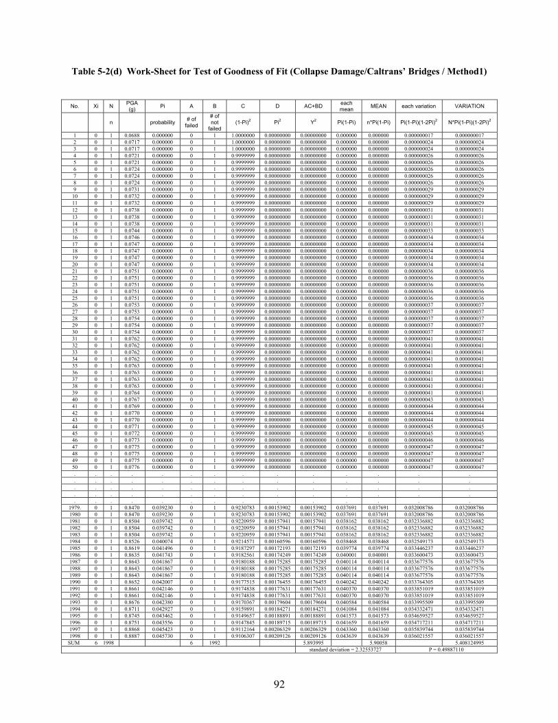
92
Table 5-2(d) Work-Sheet for Test of Goodness of Fit (Collapse Damage/Caltrans’ Bridges / Method1)
No. Xi N PGA (g) Pi A B C D AC+BD each
mean MEAN each variation VARIATION
n probability # of failed
# of not
failed (1-Pi)2 Pi2 Y2 Pi(1-Pi) n*Pi(1-Pi) Pi(1-Pi)(1-2Pi)2 N*Pi(1-Pi)(1-2Pi)2
1 0 1 0.0688 0.000000 0 1 1.0000000 0.00000000 0.00000000 0.000000 0.000000 0.000000017 0.000000017 2 0 1 0.0717 0.000000 0 1 1.0000000 0.00000000 0.00000000 0.000000 0.000000 0.000000024 0.000000024 3 0 1 0.0717 0.000000 0 1 1.0000000 0.00000000 0.00000000 0.000000 0.000000 0.000000024 0.000000024 4 0 1 0.0721 0.000000 0 1 0.9999999 0.00000000 0.00000000 0.000000 0.000000 0.000000026 0.000000026 5 0 1 0.0721 0.000000 0 1 0.9999999 0.00000000 0.00000000 0.000000 0.000000 0.000000026 0.000000026 6 0 1 0.0724 0.000000 0 1 0.9999999 0.00000000 0.00000000 0.000000 0.000000 0.000000026 0.000000026 7 0 1 0.0724 0.000000 0 1 0.9999999 0.00000000 0.00000000 0.000000 0.000000 0.000000026 0.000000026 8 0 1 0.0724 0.000000 0 1 0.9999999 0.00000000 0.00000000 0.000000 0.000000 0.000000026 0.000000026 9 0 1 0.0731 0.000000 0 1 0.9999999 0.00000000 0.00000000 0.000000 0.000000 0.000000029 0.000000029 10 0 1 0.0732 0.000000 0 1 0.9999999 0.00000000 0.00000000 0.000000 0.000000 0.000000029 0.000000029 11 0 1 0.0732 0.000000 0 1 0.9999999 0.00000000 0.00000000 0.000000 0.000000 0.000000029 0.000000029 12 0 1 0.0738 0.000000 0 1 0.9999999 0.00000000 0.00000000 0.000000 0.000000 0.000000031 0.000000031 13 0 1 0.0738 0.000000 0 1 0.9999999 0.00000000 0.00000000 0.000000 0.000000 0.000000031 0.000000031 14 0 1 0.0738 0.000000 0 1 0.9999999 0.00000000 0.00000000 0.000000 0.000000 0.000000031 0.000000031 15 0 1 0.0744 0.000000 0 1 0.9999999 0.00000000 0.00000000 0.000000 0.000000 0.000000033 0.000000033 16 0 1 0.0746 0.000000 0 1 0.9999999 0.00000000 0.00000000 0.000000 0.000000 0.000000034 0.000000034 17 0 1 0.0747 0.000000 0 1 0.9999999 0.00000000 0.00000000 0.000000 0.000000 0.000000034 0.000000034 18 0 1 0.0747 0.000000 0 1 0.9999999 0.00000000 0.00000000 0.000000 0.000000 0.000000034 0.000000034 19 0 1 0.0747 0.000000 0 1 0.9999999 0.00000000 0.00000000 0.000000 0.000000 0.000000034 0.000000034 20 0 1 0.0747 0.000000 0 1 0.9999999 0.00000000 0.00000000 0.000000 0.000000 0.000000034 0.000000034 21 0 1 0.0751 0.000000 0 1 0.9999999 0.00000000 0.00000000 0.000000 0.000000 0.000000036 0.000000036 22 0 1 0.0751 0.000000 0 1 0.9999999 0.00000000 0.00000000 0.000000 0.000000 0.000000036 0.000000036 23 0 1 0.0751 0.000000 0 1 0.9999999 0.00000000 0.00000000 0.000000 0.000000 0.000000036 0.000000036 24 0 1 0.0751 0.000000 0 1 0.9999999 0.00000000 0.00000000 0.000000 0.000000 0.000000036 0.000000036 25 0 1 0.0751 0.000000 0 1 0.9999999 0.00000000 0.00000000 0.000000 0.000000 0.000000036 0.000000036 26 0 1 0.0753 0.000000 0 1 0.9999999 0.00000000 0.00000000 0.000000 0.000000 0.000000037 0.000000037 27 0 1 0.0753 0.000000 0 1 0.9999999 0.00000000 0.00000000 0.000000 0.000000 0.000000037 0.000000037 28 0 1 0.0754 0.000000 0 1 0.9999999 0.00000000 0.00000000 0.000000 0.000000 0.000000037 0.000000037 29 0 1 0.0754 0.000000 0 1 0.9999999 0.00000000 0.00000000 0.000000 0.000000 0.000000037 0.000000037 30 0 1 0.0754 0.000000 0 1 0.9999999 0.00000000 0.00000000 0.000000 0.000000 0.000000037 0.000000037 31 0 1 0.0762 0.000000 0 1 0.9999999 0.00000000 0.00000000 0.000000 0.000000 0.000000041 0.000000041 32 0 1 0.0762 0.000000 0 1 0.9999999 0.00000000 0.00000000 0.000000 0.000000 0.000000041 0.000000041 33 0 1 0.0762 0.000000 0 1 0.9999999 0.00000000 0.00000000 0.000000 0.000000 0.000000041 0.000000041 34 0 1 0.0762 0.000000 0 1 0.9999999 0.00000000 0.00000000 0.000000 0.000000 0.000000041 0.000000041 35 0 1 0.0763 0.000000 0 1 0.9999999 0.00000000 0.00000000 0.000000 0.000000 0.000000041 0.000000041 36 0 1 0.0763 0.000000 0 1 0.9999999 0.00000000 0.00000000 0.000000 0.000000 0.000000041 0.000000041 37 0 1 0.0763 0.000000 0 1 0.9999999 0.00000000 0.00000000 0.000000 0.000000 0.000000041 0.000000041 38 0 1 0.0763 0.000000 0 1 0.9999999 0.00000000 0.00000000 0.000000 0.000000 0.000000041 0.000000041 39 0 1 0.0764 0.000000 0 1 0.9999999 0.00000000 0.00000000 0.000000 0.000000 0.000000041 0.000000041 40 0 1 0.0767 0.000000 0 1 0.9999999 0.00000000 0.00000000 0.000000 0.000000 0.000000043 0.000000043 41 0 1 0.0769 0.000000 0 1 0.9999999 0.00000000 0.00000000 0.000000 0.000000 0.000000044 0.000000044 42 0 1 0.0770 0.000000 0 1 0.9999999 0.00000000 0.00000000 0.000000 0.000000 0.000000044 0.000000044 43 0 1 0.0770 0.000000 0 1 0.9999999 0.00000000 0.00000000 0.000000 0.000000 0.000000044 0.000000044 44 0 1 0.0771 0.000000 0 1 0.9999999 0.00000000 0.00000000 0.000000 0.000000 0.000000045 0.000000045 45 0 1 0.0772 0.000000 0 1 0.9999999 0.00000000 0.00000000 0.000000 0.000000 0.000000045 0.000000045 46 0 1 0.0773 0.000000 0 1 0.9999999 0.00000000 0.00000000 0.000000 0.000000 0.000000046 0.000000046 47 0 1 0.0775 0.000000 0 1 0.9999999 0.00000000 0.00000000 0.000000 0.000000 0.000000047 0.000000047 48 0 1 0.0775 0.000000 0 1 0.9999999 0.00000000 0.00000000 0.000000 0.000000 0.000000047 0.000000047 49 0 1 0.0775 0.000000 0 1 0.9999999 0.00000000 0.00000000 0.000000 0.000000 0.000000047 0.000000047 50 0 1 0.0776 0.000000 0 1 0.9999999 0.00000000 0.00000000 0.000000 0.000000 0.000000047 0.000000047 . . . . . . . . . . . . . . . . . . . . . . . . . . . . . . . . . . . . . . . . . . . . . . . . . . . . . . . . . . . . . . . . . . . . . .
1979. 0 1 0.8470 0.039230 0 1 0.9230783 0.00153902 0.00153902 0.037691 0.037691 0.032008786 0.032008786 1980 0 1 0.8470 0.039230 0 1 0.9230783 0.00153902 0.00153902 0.037691 0.037691 0.032008786 0.032008786 1981 0 1 0.8504 0.039742 0 1 0.9220959 0.00157941 0.00157941 0.038162 0.038162 0.032336882 0.032336882 1982 0 1 0.8504 0.039742 0 1 0.9220959 0.00157941 0.00157941 0.038162 0.038162 0.032336882 0.032336882 1983 0 1 0.8504 0.039742 0 1 0.9220959 0.00157941 0.00157941 0.038162 0.038162 0.032336882 0.032336882 1984 0 1 0.8526 0.040074 0 1 0.9214571 0.00160596 0.00160596 0.038468 0.038468 0.032549173 0.032549173 1985 0 1 0.8619 0.041496 0 1 0.9187297 0.00172193 0.00172193 0.039774 0.039774 0.033446237 0.033446237 1986 0 1 0.8635 0.041743 0 1 0.9182561 0.00174249 0.00174249 0.040001 0.040001 0.033600473 0.033600473 1987 0 1 0.8643 0.041867 0 1 0.9180188 0.00175285 0.00175285 0.040114 0.040114 0.033677576 0.033677576 1988 0 1 0.8643 0.041867 0 1 0.9180188 0.00175285 0.00175285 0.040114 0.040114 0.033677576 0.033677576 1989 0 1 0.8643 0.041867 0 1 0.9180188 0.00175285 0.00175285 0.040114 0.040114 0.033677576 0.033677576 1990 0 1 0.8652 0.042007 0 1 0.9177515 0.00176455 0.00176455 0.040242 0.040242 0.033764305 0.033764305 1991 0 1 0.8661 0.042146 0 1 0.9174838 0.00177631 0.00177631 0.040370 0.040370 0.033851019 0.033851019 1992 0 1 0.8661 0.042146 0 1 0.9174838 0.00177631 0.00177631 0.040370 0.040370 0.033851019 0.033851019 1993 0 1 0.8676 0.042380 0 1 0.9170367 0.00179604 0.00179604 0.040584 0.040584 0.033995509 0.033995509 1994 0 1 0.8711 0.042927 0 1 0.9159891 0.00184271 0.00184271 0.041084 0.041084 0.034332471 0.034332471 1995 0 1 0.8745 0.043462 0 1 0.9149657 0.00188891 0.00188891 0.041573 0.041573 0.034659527 0.034659527 1996 0 1 0.8751 0.043556 0 1 0.9147845 0.00189715 0.00189715 0.041659 0.041659 0.034717211 0.034717211 1997 0 1 0.8868 0.045423 0 1 0.9112164 0.00206329 0.00206329 0.043360 0.043360 0.035839744 0.035839744 1998 0 1 0.8887 0.045730 0 1 0.9106307 0.00209126 0.00209126 0.043639 0.043639 0.036021557 0.036021557
SUM 6 1998 6 1992 5.893995 5.90058 5.408124995 standard deviation = 2.32553727 P = 0.49887110

93
Table 5-3(a) Work-Sheet for Test of Goodness of Fit (Minor Damage/HEPC’s Bridges / Method1)
No. Xi N PGA (g) Pi A B C D AC+BD each
mean MEAN each variation VARIATION
n probability # of failed
# of not
failed (1-Pi)2 Pi2 Y2 Pi(1-Pi) n*Pi(1-Pi) Pi(1-Pi)(1-2Pi)2 N*Pi(1-Pi)(1-2Pi)2
1 7 55 239.12 0.130996 7 48 0.7551687 0.01715984 6.1098532 0.113836 6.260966 0.062001438 3.410079067 2 19 55 267.60 0.175846 19 36 0.6792303 0.03092172 14.0185568 0.144924 7.970821 0.060912135 3.350167417 3 3 55 295.83 0.223149 3 52 0.6034976 0.04979545 4.3998560 0.173353 9.534442 0.053147760 2.923126809 4 3 55 376.31 0.361500 3 52 0.4076827 0.13068200 8.0185120 0.230818 12.694971 0.017710497 0.974077318 5 33 55 431.04 0.450393 33 22 0.3020679 0.20285386 14.4310240 0.247539 13.614653 0.002436631 0.134014714 6 26 55 477.50 0.519348 26 29 0.2310265 0.26972215 13.8286320 0.249626 13.729411 0.000373777 0.020557746 7 40 55 487.85 0.533800 40 15 0.2173426 0.28494227 12.9678375 0.248858 13.687166 0.001137209 0.062546484 8 41 55 504.65 0.556493 41 14 0.1966989 0.30968395 12.4002288 0.246809 13.574473 0.003150667 0.173286672 9 27 55 521.94 0.578901 27 28 0.1773241 0.33512680 14.1712998 0.243775 13.407602 0.006070402 0.333872129 10 25 55 534.82 0.594967 25 30 0.1640515 0.35398605 14.7208694 0.240981 13.253967 0.008693429 0.478138583 11 45 55 581.95 0.649230 45 10 0.1230395 0.42149973 9.7517756 0.227730 12.525171 0.020285880 1.115723396 12 44 55 604.34 0.672612 44 11 0.1071832 0.45240628 9.6925301 0.220205 12.111289 0.026243836 1.443410980 13 34 55 655.05 0.720208 34 21 0.0782837 0.51869913 13.5543286 0.201509 11.082971 0.039085755 2.149716518 14 35 55 721.85 0.772704 35 20 0.0516635 0.59707121 13.7496484 0.175633 9.659794 0.052245350 2.873494265
SUM 382 770 382 388 161.814952 163.10770 19.442212099 standard deviation = 4.40933239 P = 0.38469092
Table 5-3(b) Work-Sheet for Test of Goodness of Fit (Moderate Damage/HEPC’s Bridges / Method1)
No. Xi N PGA (g) Pi A B C D AC+BD each
mean MEAN each variation VARIATION
n probability # of failed
# of not
failed (1-Pi)2 Pi2 Y2 Pi(1-Pi) n*Pi(1-Pi) Pi(1-Pi)(1-2Pi)2 N*Pi(1-Pi)(1-2Pi)2
1 0 55 239.12 0.010382 0 55 0.9793433 0.00010779 0.0059285 0.010274 0.565096 0.009852215 0.541871849 2 1 55 267.60 0.019542 1 54 0.9612985 0.00038188 0.9819199 0.019160 1.053790 0.017691430 0.973028675 3 0 55 295.83 0.032781 0 55 0.9355123 0.00107460 0.0591031 0.031707 1.743859 0.027685312 1.522692176 4 0 55 376.31 0.095259 0 55 0.8185564 0.00907427 0.4990846 0.086185 4.740157 0.056473481 3.106041481 5 2 55 431.04 0.156583 2 53 0.7113519 0.02451831 2.7221740 0.132065 7.263571 0.062300348 3.426519116 6 11 55 477.50 0.217061 11 44 0.6129933 0.04711553 8.8160095 0.169946 9.347007 0.054419577 2.993076712 7 23 55 487.85 0.231266 23 32 0.5909515 0.05348409 15.3033762 0.177782 9.778020 0.051356162 2.824588936 8 36 55 504.65 0.254685 36 19 0.5554939 0.06486463 21.2302092 0.189821 10.440140 0.045693095 2.513120230 9 17 55 521.94 0.279177 17 38 0.5195853 0.07793998 11.7946698 0.201237 11.068054 0.039251470 2.158830842 10 12 55 534.82 0.297591 12 43 0.4933783 0.08856046 9.7286391 0.209031 11.496685 0.034255408 1.884047428 11 13 55 581.95 0.365237 13 42 0.4029239 0.13339816 10.8407334 0.231839 12.751143 0.016841741 0.926295740 12 34 55 604.34 0.397064 34 21 0.3635314 0.15766008 15.6709302 0.239404 13.167234 0.010146673 0.558067018 13 21 55 655.05 0.467042 21 34 0.2840447 0.21812782 13.3812845 0.248914 13.690256 0.001081539 0.059484640 14 17 55 721.85 0.552566 17 38 0.2001974 0.30532888 15.0058538 0.247237 13.598026 0.002732615 0.150293852
SUM 187 770 187 583 126.039916 120.70304 23.637958696 standard deviation = 4.86188839 P = 0.86383141
Table 5-3(c) Work-Sheet for Test of Goodness of Fit (Major Damage/HEPC’s Bridges / Method1)
No. Xi N PGA (g) Pi A B C D AC+BD each
mean MEAN each variation VARIATION
n probability # of failed
# of not
failed (1-Pi)2 Pi2 Y2 Pi(1-Pi) n*Pi(1-Pi) Pi(1-Pi)(1-2Pi)2 N*Pi(1-Pi)(1-2Pi)2
1 0 55 239.12 0.003129 0 55 0.9937510 0.00000979 0.0005386 0.003120 0.171578 0.003080677 0.169437242 2 0 55 267.60 0.006691 0 55 0.9866634 0.00004477 0.0024621 0.006646 0.365526 0.006469249 0.355808681 3 0 55 295.83 0.012504 0 55 0.9751485 0.00015635 0.0085992 0.012348 0.679118 0.011737739 0.645575656 4 0 55 376.31 0.046064 0 55 0.9099941 0.00212188 0.1167035 0.043942 2.416810 0.036218403 1.992012167 5 2 55 431.04 0.085356 2 53 0.8365737 0.00728564 2.0592864 0.078070 4.293868 0.053690423 2.952973286 6 7 55 477.50 0.128609 7 48 0.7593231 0.01654016 6.1091891 0.112068 6.163762 0.061831094 3.400710176 7 10 55 487.85 0.139333 10 45 0.7407478 0.01941366 8.2810930 0.119919 6.595559 0.062396744 3.431820932 8 26 55 504.65 0.157451 26 29 0.7098892 0.02479074 19.1760515 0.132660 7.296301 0.062265297 3.424591320 9 10 55 521.94 0.176961 10 45 0.6773934 0.03131514 8.1831158 0.145646 8.010514 0.060795019 3.343726058 10 4 55 534.82 0.191996 4 51 0.6528712 0.03686228 4.4914612 0.155133 8.532328 0.058867951 3.237737327 11 6 55 581.95 0.249816 6 49 0.5627764 0.06240793 6.4346466 0.187408 10.307432 0.046921036 2.580656971 12 27 55 604.34 0.278380 27 28 0.5207351 0.07749554 16.2297234 0.200885 11.048657 0.039466068 2.170633753 13 16 55 655.05 0.344150 16 39 0.4301392 0.11843923 11.5013573 0.225711 12.414093 0.021929355 1.206114550 14 16 55 721.85 0.430005 16 39 0.3248943 0.18490430 12.4095765 0.245101 13.480539 0.004803287 0.264180808
SUM 124 770 124 646 95.0038042 91.776084 29.175978924 standard deviation = 5.40147933 P = 0.72493405

94
Table 5-4(a) Work-Sheet for Test of Goodness of Fit (Minor Damage/Memphis Bridge1 / Method1)
No. Xi N PGA (g) Pi A B C D AC+BD each
mean MEAN each variation VARIATION
n probability # of failed
# of not
failed (1-Pi)2 Pi2 Y2 Pi(1-Pi) n*Pi(1-Pi) Pi(1-Pi)(1-
2Pi)2 N*Pi(1-Pi)(1-2Pi)2
1 0 1 0.0820 0.000001 0 1 0.9999985 0.00000000 0.00000000 0.000001 0.000001 0.000000739 0.000000739 2 0 1 0.0900 0.000009 0 1 0.9999829 0.00000000 0.00000000 0.000009 0.000009 0.000008545 0.000008545 3 0 1 0.0960 0.000040 0 1 0.9999197 0.00000000 0.00000000 0.000040 0.000040 0.000040166 0.000040166 4 0 1 0.0970 0.000051 0 1 0.9998981 0.00000000 0.00000000 0.000051 0.000051 0.000050918 0.000050918 5 0 1 0.0980 0.000064 0 1 0.9998716 0.00000000 0.00000000 0.000064 0.000064 0.000064193 0.000064193 6 0 1 0.0980 0.000064 0 1 0.9998716 0.00000000 0.00000000 0.000064 0.000064 0.000064193 0.000064193 7 0 1 0.1070 0.000413 0 1 0.9991746 0.00000017 0.00000017 0.000413 0.000413 0.000411923 0.000411923 8 0 1 0.1090 0.000594 0 1 0.9988125 0.00000035 0.00000035 0.000594 0.000594 0.000592175 0.000592175 9 0 1 0.1100 0.000708 0 1 0.9985843 0.00000050 0.00000050 0.000708 0.000708 0.000705609 0.000705609 10 0 1 0.1140 0.001377 0 1 0.9972484 0.00000190 0.00000190 0.001375 0.001375 0.001367288 0.001367288 11 0 1 0.1140 0.001377 0 1 0.9972484 0.00000190 0.00000190 0.001375 0.001375 0.001367288 0.001367288 12 0 1 0.1170 0.002183 0 1 0.9956396 0.00000476 0.00000476 0.002178 0.002178 0.002158848 0.002158848 13 0 1 0.1210 0.003852 0 1 0.9923107 0.00001484 0.00001484 0.003837 0.003837 0.003778312 0.003778312 14 0 1 0.1220 0.004406 0 1 0.9912083 0.00001941 0.00001941 0.004386 0.004386 0.004309175 0.004309175 15 0 1 0.1240 0.005712 0 1 0.9886089 0.00003263 0.00003263 0.005679 0.005679 0.005550215 0.005550215 16 0 1 0.1270 0.008256 0 1 0.9835558 0.00006816 0.00006816 0.008188 0.008188 0.007919826 0.007919826 17 0 1 0.1320 0.014479 0 1 0.9712511 0.00020965 0.00020965 0.014270 0.014270 0.013455158 0.013455158 18 0 1 0.1350 0.019705 0 1 0.9609792 0.00038827 0.00038827 0.019316 0.019316 0.017823779 0.017823779 19 0 1 0.1390 0.028811 0 1 0.9432088 0.00083005 0.00083005 0.027981 0.027981 0.024848914 0.024848914 20 0 1 0.1400 0.031516 0 1 0.9379610 0.00099327 0.00099327 0.030523 0.030523 0.026796300 0.026796300 21 0 1 0.1410 0.034407 0 1 0.9323700 0.00118383 0.00118383 0.033223 0.033223 0.028807974 0.028807974 22 0 1 0.1450 0.047948 0 1 0.9064038 0.00229897 0.00229897 0.045649 0.045649 0.037313430 0.037313430 23 0 1 0.1550 0.097380 0 1 0.8147232 0.00948282 0.00948282 0.087897 0.087897 0.056993460 0.056993460 24 0 1 0.1620 0.146265 0 1 0.7288633 0.02139348 0.02139348 0.124872 0.124872 0.062499934 0.062499934 25 1 1 0.1700 0.215852 1 0 0.6148874 0.04659226 0.61488745 0.169260 0.169260 0.054664158 0.054664158 26 0 1 0.1730 0.245213 0 1 0.5697029 0.06012957 0.06012957 0.185084 0.185084 0.048059774 0.048059774 27 1 1 0.1730 0.245213 1 0 0.5697029 0.06012957 0.56970294 0.185084 0.185084 0.048059774 0.048059774 28 0 1 0.1750 0.265616 0 1 0.5393194 0.07055202 0.07055202 0.195064 0.195064 0.042863984 0.042863984 29 1 1 0.1750 0.265616 1 0 0.5393194 0.07055202 0.53931941 0.195064 0.195064 0.042863984 0.042863984 30 0 1 0.1920 0.454651 0 1 0.2974055 0.20670759 0.20670759 0.247943 0.247943 0.002039609 0.002039609 31 0 1 0.1930 0.466044 0 1 0.2851091 0.21719696 0.21719696 0.248847 0.248847 0.001147696 0.001147696 32 0 1 0.1970 0.511215 0 1 0.2389104 0.26134118 0.26134118 0.249874 0.249874 0.000125722 0.000125722 33 1 1 0.2080 0.628660 1 0 0.1378935 0.39521321 0.13789350 0.233447 0.233447 0.015457303 0.015457303 34 1 1 0.2170 0.713056 1 0 0.0823367 0.50844922 0.08233672 0.204607 0.204607 0.037150881 0.037150881 35 0 1 0.2200 0.738326 0 1 0.0684733 0.54512522 0.54512522 0.193201 0.193201 0.043894637 0.043894637 36 1 1 0.2200 0.738326 1 0 0.0684733 0.54512522 0.06847331 0.193201 0.193201 0.043894637 0.043894637 37 1 1 0.2210 0.746414 1 0 0.0643056 0.55713457 0.06430562 0.189280 0.189280 0.045972375 0.045972375 38 0 1 0.2230 0.762084 0 1 0.0566039 0.58077237 0.58077237 0.181312 0.181312 0.049815898 0.049815898 39 1 1 0.2330 0.830307 1 0 0.0287956 0.68941013 0.02879563 0.140897 0.140897 0.061489126 0.061489126 40 1 1 0.2330 0.830307 1 0 0.0287956 0.68941013 0.02879563 0.140897 0.140897 0.061489126 0.061489126 41 1 1 0.2380 0.858294 1 0 0.0200807 0.73666819 0.02008066 0.121626 0.121626 0.062454453 0.062454453 42 1 1 0.2430 0.882495 1 0 0.0138075 0.77879711 0.01380747 0.103698 0.103698 0.060684850 0.060684850 43 0 1 0.2480 0.903213 0 1 0.0093678 0.81579334 0.81579334 0.087419 0.087419 0.056850809 0.056850809 44 1 1 0.2520 0.917504 1 0 0.0068056 0.84181377 0.00680557 0.075690 0.075690 0.052774224 0.052774224 45 1 1 0.2540 0.923950 1 0 0.0057836 0.85368336 0.00578362 0.070267 0.070267 0.050516980 0.050516980 46 1 1 0.2550 0.927008 1 0 0.0053279 0.85934304 0.00532789 0.067665 0.067665 0.049350578 0.049350578 47 1 1 0.2570 0.932807 1 0 0.0045150 0.87012801 0.00451496 0.062679 0.062679 0.046964129 0.046964129 48 1 1 0.2580 0.935553 1 0 0.0041534 0.87525996 0.00415338 0.060293 0.060293 0.045752188 0.045752188 49 1 1 0.2590 0.938202 1 0 0.0038190 0.88022280 0.00381901 0.057979 0.057979 0.044532795 0.044532795 50 1 1 0.2720 0.964885 1 0 0.0012330 0.93100366 0.00123304 0.033882 0.033882 0.029289785 0.029289785 . . . . . . . . . . . . . . . . . . . . . . . . . . . . . . . . . . . . . . . . . . . . . . . . . . . . . . . . . . . . . . . . . . . . . .
61 1 1 0.3110 0.994625 1 0 0.0000289 0.98927843 0.00002889 0.005346 0.005346 0.005232007 0.005232007 62 1 1 0.3140 0.995389 1 0 0.0000213 0.99080013 0.00002126 0.004589 0.004589 0.004505061 0.004505061 63 1 1 0.3240 0.997256 1 0 0.0000075 0.99452033 0.00000753 0.002736 0.002736 0.002706125 0.002706125 64 1 1 0.3320 0.998203 1 0 0.0000032 0.99640858 0.00000323 0.001794 0.001794 0.001781217 0.001781217 65 1 1 0.3320 0.998203 1 0 0.0000032 0.99640858 0.00000323 0.001794 0.001794 0.001781217 0.001781217 66 1 1 0.3450 0.999108 1 0 0.0000008 0.99821608 0.00000080 0.000892 0.000892 0.000888382 0.000888382 67 1 1 0.3550 0.999484 1 0 0.0000003 0.99896863 0.00000027 0.000516 0.000516 0.000514491 0.000514491 68 1 1 0.3570 0.999538 1 0 0.0000002 0.99907651 0.00000021 0.000462 0.000462 0.000460787 0.000460787 69 1 1 0.3610 0.999630 1 0 0.0000001 0.99926022 0.00000014 0.000370 0.000370 0.000369276 0.000369276 70 1 1 0.3680 0.999750 1 0 0.0000001 0.99949947 0.00000006 0.000250 0.000250 0.000249983 0.000249983 71 1 1 0.3720 0.999800 1 0 0.0000000 0.99960016 0.00000004 0.000200 0.000200 0.000199741 0.000199741 72 1 1 0.3830 0.999893 1 0 0.0000000 0.99978538 0.00000001 0.000107 0.000107 0.000107257 0.000107257 73 1 1 0.3830 0.999893 1 0 0.0000000 0.99978538 0.00000001 0.000107 0.000107 0.000107257 0.000107257 74 1 1 0.3840 0.999899 1 0 0.0000000 0.99979725 0.00000001 0.000101 0.000101 0.000101330 0.000101330 75 1 1 0.3890 0.999924 1 0 0.0000000 0.99984754 0.00000001 0.000076 0.000076 0.000076205 0.000076205 76 1 1 0.3890 0.999924 1 0 0.0000000 0.99984754 0.00000001 0.000076 0.000076 0.000076205 0.000076205 77 1 1 0.3900 0.999928 1 0 0.0000000 0.99985601 0.00000001 0.000072 0.000072 0.000071973 0.000071973 78 1 1 0.4240 0.999990 1 0 0.0000000 0.99997982 0.00000000 0.000010 0.000010 0.000010087 0.000010087 79 1 1 0.4300 0.999993 1 0 0.0000000 0.99998579 0.00000000 0.000007 0.000007 0.000007106 0.000007106 80 1 1 0.4680 0.999999 1 0 0.0000000 0.99999848 0.00000000 0.000001 0.000001 0.000000761 0.000000761
SUM 48 80 48 32 4.99635960 4.510080 1.532224182 standard deviation = 1.23783043 P = 0.63905036
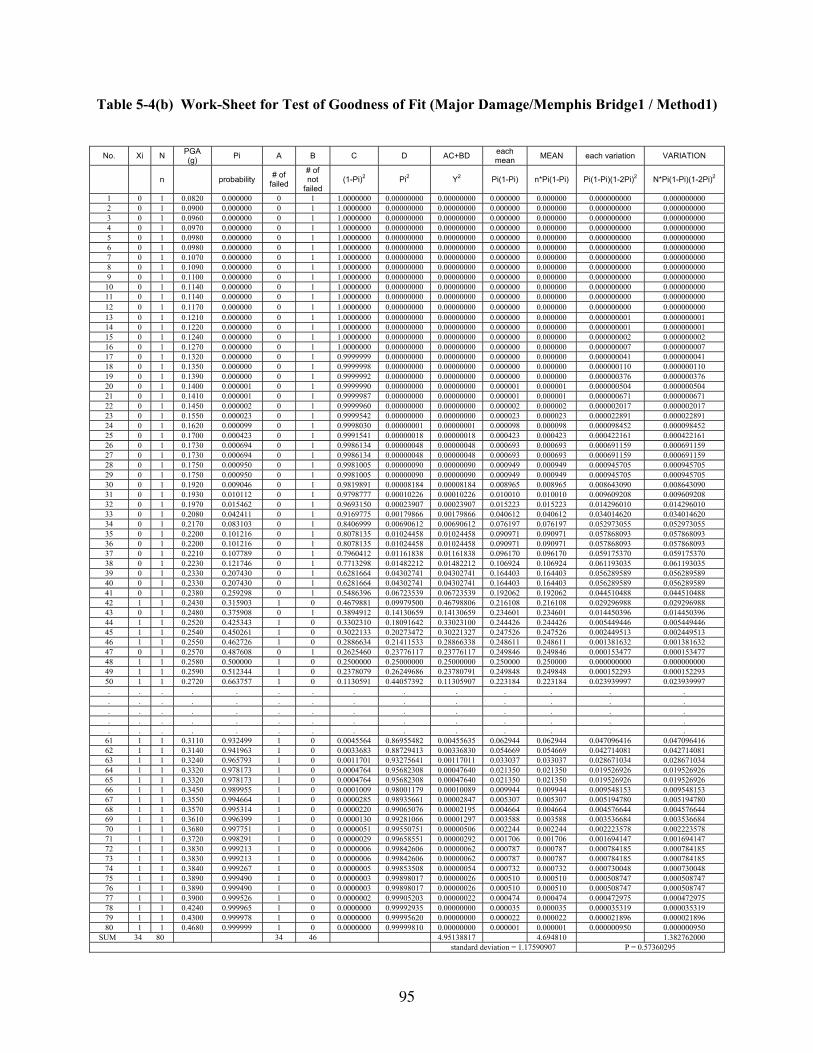
95
Table 5-4(b) Work-Sheet for Test of Goodness of Fit (Major Damage/Memphis Bridge1 / Method1)
No. Xi N PGA (g) Pi A B C D AC+BD each
mean MEAN each variation VARIATION
n probability # of failed
# of not
failed (1-Pi)2 Pi2 Y2 Pi(1-Pi) n*Pi(1-Pi) Pi(1-Pi)(1-2Pi)2 N*Pi(1-Pi)(1-2Pi)2
1 0 1 0.0820 0.000000 0 1 1.0000000 0.00000000 0.00000000 0.000000 0.000000 0.000000000 0.000000000 2 0 1 0.0900 0.000000 0 1 1.0000000 0.00000000 0.00000000 0.000000 0.000000 0.000000000 0.000000000 3 0 1 0.0960 0.000000 0 1 1.0000000 0.00000000 0.00000000 0.000000 0.000000 0.000000000 0.000000000 4 0 1 0.0970 0.000000 0 1 1.0000000 0.00000000 0.00000000 0.000000 0.000000 0.000000000 0.000000000 5 0 1 0.0980 0.000000 0 1 1.0000000 0.00000000 0.00000000 0.000000 0.000000 0.000000000 0.000000000 6 0 1 0.0980 0.000000 0 1 1.0000000 0.00000000 0.00000000 0.000000 0.000000 0.000000000 0.000000000 7 0 1 0.1070 0.000000 0 1 1.0000000 0.00000000 0.00000000 0.000000 0.000000 0.000000000 0.000000000 8 0 1 0.1090 0.000000 0 1 1.0000000 0.00000000 0.00000000 0.000000 0.000000 0.000000000 0.000000000 9 0 1 0.1100 0.000000 0 1 1.0000000 0.00000000 0.00000000 0.000000 0.000000 0.000000000 0.000000000 10 0 1 0.1140 0.000000 0 1 1.0000000 0.00000000 0.00000000 0.000000 0.000000 0.000000000 0.000000000 11 0 1 0.1140 0.000000 0 1 1.0000000 0.00000000 0.00000000 0.000000 0.000000 0.000000000 0.000000000 12 0 1 0.1170 0.000000 0 1 1.0000000 0.00000000 0.00000000 0.000000 0.000000 0.000000000 0.000000000 13 0 1 0.1210 0.000000 0 1 1.0000000 0.00000000 0.00000000 0.000000 0.000000 0.000000001 0.000000001 14 0 1 0.1220 0.000000 0 1 1.0000000 0.00000000 0.00000000 0.000000 0.000000 0.000000001 0.000000001 15 0 1 0.1240 0.000000 0 1 1.0000000 0.00000000 0.00000000 0.000000 0.000000 0.000000002 0.000000002 16 0 1 0.1270 0.000000 0 1 1.0000000 0.00000000 0.00000000 0.000000 0.000000 0.000000007 0.000000007 17 0 1 0.1320 0.000000 0 1 0.9999999 0.00000000 0.00000000 0.000000 0.000000 0.000000041 0.000000041 18 0 1 0.1350 0.000000 0 1 0.9999998 0.00000000 0.00000000 0.000000 0.000000 0.000000110 0.000000110 19 0 1 0.1390 0.000000 0 1 0.9999992 0.00000000 0.00000000 0.000000 0.000000 0.000000376 0.000000376 20 0 1 0.1400 0.000001 0 1 0.9999990 0.00000000 0.00000000 0.000001 0.000001 0.000000504 0.000000504 21 0 1 0.1410 0.000001 0 1 0.9999987 0.00000000 0.00000000 0.000001 0.000001 0.000000671 0.000000671 22 0 1 0.1450 0.000002 0 1 0.9999960 0.00000000 0.00000000 0.000002 0.000002 0.000002017 0.000002017 23 0 1 0.1550 0.000023 0 1 0.9999542 0.00000000 0.00000000 0.000023 0.000023 0.000022891 0.000022891 24 0 1 0.1620 0.000099 0 1 0.9998030 0.00000001 0.00000001 0.000098 0.000098 0.000098452 0.000098452 25 0 1 0.1700 0.000423 0 1 0.9991541 0.00000018 0.00000018 0.000423 0.000423 0.000422161 0.000422161 26 0 1 0.1730 0.000694 0 1 0.9986134 0.00000048 0.00000048 0.000693 0.000693 0.000691159 0.000691159 27 0 1 0.1730 0.000694 0 1 0.9986134 0.00000048 0.00000048 0.000693 0.000693 0.000691159 0.000691159 28 0 1 0.1750 0.000950 0 1 0.9981005 0.00000090 0.00000090 0.000949 0.000949 0.000945705 0.000945705 29 0 1 0.1750 0.000950 0 1 0.9981005 0.00000090 0.00000090 0.000949 0.000949 0.000945705 0.000945705 30 0 1 0.1920 0.009046 0 1 0.9819891 0.00008184 0.00008184 0.008965 0.008965 0.008643090 0.008643090 31 0 1 0.1930 0.010112 0 1 0.9798777 0.00010226 0.00010226 0.010010 0.010010 0.009609208 0.009609208 32 0 1 0.1970 0.015462 0 1 0.9693150 0.00023907 0.00023907 0.015223 0.015223 0.014296010 0.014296010 33 0 1 0.2080 0.042411 0 1 0.9169775 0.00179866 0.00179866 0.040612 0.040612 0.034014620 0.034014620 34 0 1 0.2170 0.083103 0 1 0.8406999 0.00690612 0.00690612 0.076197 0.076197 0.052973055 0.052973055 35 0 1 0.2200 0.101216 0 1 0.8078135 0.01024458 0.01024458 0.090971 0.090971 0.057868093 0.057868093 36 0 1 0.2200 0.101216 0 1 0.8078135 0.01024458 0.01024458 0.090971 0.090971 0.057868093 0.057868093 37 0 1 0.2210 0.107789 0 1 0.7960412 0.01161838 0.01161838 0.096170 0.096170 0.059175370 0.059175370 38 0 1 0.2230 0.121746 0 1 0.7713298 0.01482212 0.01482212 0.106924 0.106924 0.061193035 0.061193035 39 0 1 0.2330 0.207430 0 1 0.6281664 0.04302741 0.04302741 0.164403 0.164403 0.056289589 0.056289589 40 0 1 0.2330 0.207430 0 1 0.6281664 0.04302741 0.04302741 0.164403 0.164403 0.056289589 0.056289589 41 0 1 0.2380 0.259298 0 1 0.5486396 0.06723539 0.06723539 0.192062 0.192062 0.044510488 0.044510488 42 1 1 0.2430 0.315903 1 0 0.4679881 0.09979500 0.46798806 0.216108 0.216108 0.029296988 0.029296988 43 0 1 0.2480 0.375908 0 1 0.3894912 0.14130659 0.14130659 0.234601 0.234601 0.014450396 0.014450396 44 1 1 0.2520 0.425343 1 0 0.3302310 0.18091642 0.33023100 0.244426 0.244426 0.005449446 0.005449446 45 1 1 0.2540 0.450261 1 0 0.3022133 0.20273472 0.30221327 0.247526 0.247526 0.002449513 0.002449513 46 1 1 0.2550 0.462726 1 0 0.2886634 0.21411533 0.28866338 0.248611 0.248611 0.001381632 0.001381632 47 0 1 0.2570 0.487608 0 1 0.2625460 0.23776117 0.23776117 0.249846 0.249846 0.000153477 0.000153477 48 1 1 0.2580 0.500000 1 0 0.2500000 0.25000000 0.25000000 0.250000 0.250000 0.000000000 0.000000000 49 1 1 0.2590 0.512344 1 0 0.2378079 0.26249686 0.23780791 0.249848 0.249848 0.000152293 0.000152293 50 1 1 0.2720 0.663757 1 0 0.1130591 0.44057392 0.11305907 0.223184 0.223184 0.023939997 0.023939997 . . . . . . . . . . . . . . . . . . . . . . . . . . . . . . . . . . . . . . . . . . . . . . . . . . . . . . . . . . . . . . . . . . . . . .
61 1 1 0.3110 0.932499 1 0 0.0045564 0.86955482 0.00455635 0.062944 0.062944 0.047096416 0.047096416 62 1 1 0.3140 0.941963 1 0 0.0033683 0.88729413 0.00336830 0.054669 0.054669 0.042714081 0.042714081 63 1 1 0.3240 0.965793 1 0 0.0011701 0.93275641 0.00117011 0.033037 0.033037 0.028671034 0.028671034 64 1 1 0.3320 0.978173 1 0 0.0004764 0.95682308 0.00047640 0.021350 0.021350 0.019526926 0.019526926 65 1 1 0.3320 0.978173 1 0 0.0004764 0.95682308 0.00047640 0.021350 0.021350 0.019526926 0.019526926 66 1 1 0.3450 0.989955 1 0 0.0001009 0.98001179 0.00010089 0.009944 0.009944 0.009548153 0.009548153 67 1 1 0.3550 0.994664 1 0 0.0000285 0.98935661 0.00002847 0.005307 0.005307 0.005194780 0.005194780 68 1 1 0.3570 0.995314 1 0 0.0000220 0.99065076 0.00002195 0.004664 0.004664 0.004576644 0.004576644 69 1 1 0.3610 0.996399 1 0 0.0000130 0.99281066 0.00001297 0.003588 0.003588 0.003536684 0.003536684 70 1 1 0.3680 0.997751 1 0 0.0000051 0.99550751 0.00000506 0.002244 0.002244 0.002223578 0.002223578 71 1 1 0.3720 0.998291 1 0 0.0000029 0.99658551 0.00000292 0.001706 0.001706 0.001694147 0.001694147 72 1 1 0.3830 0.999213 1 0 0.0000006 0.99842606 0.00000062 0.000787 0.000787 0.000784185 0.000784185 73 1 1 0.3830 0.999213 1 0 0.0000006 0.99842606 0.00000062 0.000787 0.000787 0.000784185 0.000784185 74 1 1 0.3840 0.999267 1 0 0.0000005 0.99853508 0.00000054 0.000732 0.000732 0.000730048 0.000730048 75 1 1 0.3890 0.999490 1 0 0.0000003 0.99898017 0.00000026 0.000510 0.000510 0.000508747 0.000508747 76 1 1 0.3890 0.999490 1 0 0.0000003 0.99898017 0.00000026 0.000510 0.000510 0.000508747 0.000508747 77 1 1 0.3900 0.999526 1 0 0.0000002 0.99905203 0.00000022 0.000474 0.000474 0.000472975 0.000472975 78 1 1 0.4240 0.999965 1 0 0.0000000 0.99992935 0.00000000 0.000035 0.000035 0.000035319 0.000035319 79 1 1 0.4300 0.999978 1 0 0.0000000 0.99995620 0.00000000 0.000022 0.000022 0.000021896 0.000021896 80 1 1 0.4680 0.999999 1 0 0.0000000 0.99999810 0.00000000 0.000001 0.000001 0.000000950 0.000000950
SUM 34 80 34 46 4.95138817 4.694810 1.382762000 standard deviation = 1.17590907 P = 0.57360295

96
Table 5-5(a) Work-Sheet for Test of Goodness of Fit (Minor Damage/Memphis Bridge2 / Method1)
No. Xi N PGA (g) Pi A B C D AC+BD each
mean MEAN each variation VARIATION
n probability # of failed
# of not
failed (1-Pi)2 Pi2 Y2 Pi(1-Pi) n*Pi(1-Pi) Pi(1-Pi)(1-
2Pi)2 N*Pi(1-Pi)(1-2Pi)2
1 0 1 0.0820 0.000000 0 1 0.9999995 0.00000000 0.00000000 0.000000 0.000000 0.000000228 0.000000228 2 0 1 0.0900 0.000002 0 1 0.9999954 0.00000000 0.00000000 0.000002 0.000002 0.000002319 0.000002319 3 0 1 0.0960 0.000010 0 1 0.9999795 0.00000000 0.00000000 0.000010 0.000010 0.000010244 0.000010244 4 0 1 0.0970 0.000013 0 1 0.9999742 0.00000000 0.00000000 0.000013 0.000013 0.000012885 0.000012885 5 0 1 0.0980 0.000016 0 1 0.9999677 0.00000000 0.00000000 0.000016 0.000016 0.000016127 0.000016127 6 0 1 0.0980 0.000016 0 1 0.9999677 0.00000000 0.00000000 0.000016 0.000016 0.000016127 0.000016127 7 0 1 0.1070 0.000100 0 1 0.9998007 0.00000001 0.00000001 0.000100 0.000100 0.000099618 0.000099618 8 0 1 0.1090 0.000143 0 1 0.9997141 0.00000002 0.00000002 0.000143 0.000143 0.000142858 0.000142858 9 0 1 0.1100 0.000170 0 1 0.9996594 0.00000003 0.00000003 0.000170 0.000170 0.000170145 0.000170145 10 0 1 0.1140 0.000331 0 1 0.9993375 0.00000011 0.00000011 0.000331 0.000331 0.000330736 0.000330736 11 0 1 0.1140 0.000331 0 1 0.9993375 0.00000011 0.00000011 0.000331 0.000331 0.000330736 0.000330736 12 0 1 0.1170 0.000528 0 1 0.9989451 0.00000028 0.00000028 0.000527 0.000527 0.000526179 0.000526179 13 0 1 0.1210 0.000941 0 1 0.9981183 0.00000089 0.00000089 0.000940 0.000940 0.000936857 0.000936857 14 0 1 0.1220 0.001080 0 1 0.9978405 0.00000117 0.00000117 0.001079 0.001079 0.001074493 0.001074493 15 0 1 0.1240 0.001412 0 1 0.9971784 0.00000199 0.00000199 0.001410 0.001410 0.001401839 0.001401839 16 0 1 0.1270 0.002069 0 1 0.9958656 0.00000428 0.00000428 0.002065 0.002065 0.002048006 0.002048006 17 0 1 0.1320 0.003733 0 1 0.9925474 0.00001394 0.00001394 0.003719 0.003719 0.003664018 0.003664018 18 0 1 0.1350 0.005181 0 1 0.9896640 0.00002685 0.00002685 0.005155 0.005155 0.005048281 0.005048281 19 0 1 0.1390 0.007798 0 1 0.9844639 0.00006082 0.00006082 0.007738 0.007738 0.007498143 0.007498143 20 0 1 0.1400 0.008597 0 1 0.9828807 0.00007390 0.00007390 0.008523 0.008523 0.008232139 0.008232139 21 0 1 0.1410 0.009459 0 1 0.9811714 0.00008947 0.00008947 0.009370 0.009370 0.009018427 0.009018427 22 0 1 0.1450 0.013623 0 1 0.9729391 0.00018559 0.00018559 0.013438 0.013438 0.012715382 0.012715382 23 0 1 0.1550 0.030316 0 1 0.9402871 0.00091906 0.00091906 0.029397 0.029397 0.025940222 0.025940222 24 0 1 0.1620 0.048819 0 1 0.9047448 0.00238332 0.00238332 0.046436 0.046436 0.037810755 0.037810755 25 1 1 0.1700 0.078300 1 0 0.8495308 0.00613089 0.84953083 0.072169 0.072169 0.051335599 0.051335599 26 0 1 0.1730 0.091830 0 1 0.8247724 0.00843278 0.00843278 0.083397 0.083397 0.055576897 0.055576897 27 0 1 0.1730 0.091830 0 1 0.8247724 0.00843278 0.00843278 0.083397 0.083397 0.055576897 0.055576897 28 0 1 0.1750 0.101619 0 1 0.8070892 0.01032633 0.01032633 0.091292 0.091292 0.057955145 0.057955145 29 0 1 0.1750 0.101619 0 1 0.8070892 0.01032633 0.01032633 0.091292 0.091292 0.057955145 0.057955145 30 0 1 0.1920 0.208642 0 1 0.6262477 0.04353143 0.04353143 0.165110 0.165110 0.056064608 0.056064608 31 0 1 0.1930 0.216139 0 1 0.6144373 0.04671628 0.04671628 0.169423 0.169423 0.054606312 0.054606312 32 0 1 0.1970 0.247227 0 1 0.5666665 0.06112143 0.06112143 0.186106 0.186106 0.047564201 0.047564201 33 1 1 0.2080 0.339833 1 0 0.4358209 0.11548623 0.43582092 0.224346 0.224346 0.023021154 0.023021154 34 1 1 0.2170 0.419889 1 0 0.3365287 0.17630683 0.33652869 0.243582 0.243582 0.006253011 0.006253011 35 0 1 0.2200 0.446753 0 1 0.3060817 0.19958867 0.19958867 0.247165 0.247165 0.002803039 0.002803039 36 0 1 0.2200 0.446753 0 1 0.3060817 0.19958867 0.19958867 0.247165 0.247165 0.002803039 0.002803039 37 0 1 0.2210 0.455687 0 1 0.2962764 0.20765083 0.20765083 0.248036 0.248036 0.001948200 0.001948200 38 0 1 0.2230 0.473496 0 1 0.2772062 0.22419874 0.22419874 0.249298 0.249298 0.000700473 0.000700473 39 0 1 0.2330 0.560311 0 1 0.1933262 0.31394875 0.31394875 0.246363 0.246363 0.003584529 0.003584529 40 1 1 0.2330 0.560311 1 0 0.1933262 0.31394875 0.19332615 0.246363 0.246363 0.003584529 0.003584529 41 1 1 0.2380 0.601562 1 0 0.1587531 0.36187640 0.15875313 0.239685 0.239685 0.009889187 0.009889187 42 1 1 0.2430 0.640886 1 0 0.1289629 0.41073481 0.12896290 0.230151 0.230151 0.018272945 0.018272945 43 0 1 0.2480 0.678016 0 1 0.1036737 0.45970564 0.45970564 0.218310 0.218310 0.027672737 0.027672737 44 1 1 0.2520 0.706009 1 0 0.0864309 0.49844824 0.08643090 0.207560 0.207560 0.035235102 0.035235102 45 1 1 0.2540 0.719410 1 0 0.0787305 0.51755139 0.07873050 0.201859 0.201859 0.038870742 0.038870742 46 1 1 0.2550 0.725960 1 0 0.0750979 0.52701792 0.07509792 0.198942 0.198942 0.040630277 0.040630277 47 1 1 0.2570 0.738754 1 0 0.0682496 0.54575714 0.06824959 0.192997 0.192997 0.044005830 0.044005830 48 1 1 0.2580 0.744997 1 0 0.0650264 0.55502084 0.06502642 0.189976 0.189976 0.045612286 0.045612286 49 1 1 0.2590 0.751138 1 0 0.0619323 0.56420827 0.06193230 0.186930 0.186930 0.047158842 0.047158842 50 1 1 0.2720 0.821664 1 0 0.0318036 0.67513247 0.03180357 0.146532 0.146532 0.060645495 0.060645495 . . . . . . . . . . . . . . . . . . . . . . . . . . . . . . . . . . . . . . . . . . . . . . . . . . . . . . . . . . . . . . . . . . . . . .
61 1 1 0.3110 0.943896 1 0 0.0031476 0.89093993 0.00314764 0.052956 0.052956 0.041738771 0.041738771 62 1 1 0.3140 0.949092 1 0 0.0025917 0.90077499 0.00259166 0.048317 0.048317 0.038978672 0.038978672 63 1 1 0.3240 0.963440 1 0 0.0013366 0.92821692 0.00133662 0.035223 0.035223 0.030260524 0.030260524 64 1 1 0.3320 0.972154 1 0 0.0007754 0.94508287 0.00077541 0.027071 0.027071 0.024139533 0.024139533 65 1 1 0.3320 0.972154 1 0 0.0007754 0.94508287 0.00077541 0.027071 0.027071 0.024139533 0.024139533 66 1 1 0.3450 0.982334 1 0 0.0003121 0.96497950 0.00031210 0.017354 0.017354 0.016149527 0.016149527 67 1 1 0.3550 0.987670 1 0 0.0001520 0.97549166 0.00015203 0.012178 0.012178 0.011584922 0.011584922 68 1 1 0.3570 0.988536 1 0 0.0001314 0.97720340 0.00013142 0.011333 0.011333 0.010818877 0.010818877 69 1 1 0.3610 0.990099 1 0 0.0000980 0.98029534 0.00009804 0.009803 0.009803 0.009418893 0.009418893 70 1 1 0.3680 0.992359 1 0 0.0000584 0.98477578 0.00005839 0.007583 0.007583 0.007352914 0.007352914 71 1 1 0.3720 0.993420 1 0 0.0000433 0.98688282 0.00004330 0.006537 0.006537 0.006366016 0.006366016 72 1 1 0.3830 0.995660 1 0 0.0000188 0.99133803 0.00001884 0.004322 0.004322 0.004246864 0.004246864 73 1 1 0.3830 0.995660 1 0 0.0000188 0.99133803 0.00001884 0.004322 0.004322 0.004246864 0.004246864 74 1 1 0.3840 0.995822 1 0 0.0000175 0.99166174 0.00001745 0.004160 0.004160 0.004091166 0.004091166 75 1 1 0.3890 0.996551 1 0 0.0000119 0.99311347 0.00001190 0.003437 0.003437 0.003390054 0.003390054 76 1 1 0.3890 0.996551 1 0 0.0000119 0.99311347 0.00001190 0.003437 0.003437 0.003390054 0.003390054 77 1 1 0.3900 0.996681 1 0 0.0000110 0.99337305 0.00001102 0.003308 0.003308 0.003264197 0.003264197 78 1 1 0.4240 0.999127 1 0 0.0000008 0.99825459 0.00000076 0.000872 0.000872 0.000869280 0.000869280 79 1 1 0.4300 0.999313 1 0 0.0000005 0.99862726 0.00000047 0.000686 0.000686 0.000684252 0.000684252 80 1 1 0.4680 0.999854 1 0 0.0000000 0.99970712 0.00000002 0.000146 0.000146 0.000146345 0.000146345
SUM 41 80 41 39 6.08694493 6.174071 1.767572433 standard deviation = 1.32950085 P = 0.48034346
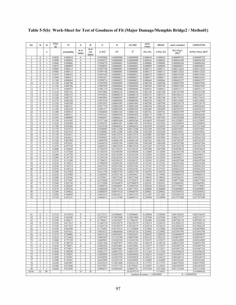
97
Table 5-5(b) Work-Sheet for Test of Goodness of Fit (Major Damage/Memphis Bridge2 / Method1)
No. Xi N PGA (g) Pi A B C D AC+BD each
mean MEAN each variation VARIATION
n probability # of failed
# of not
failed (1-Pi)2 Pi2 Y2 Pi(1-Pi) n*Pi(1-Pi) Pi(1-Pi)(1-
2Pi)2 N*Pi(1-Pi)(1-2Pi)2
1 0 1 0.0820 0.000010 0 1 0.9999806 0.00000000 0.00000000 0.000010 0.000010 0.000009724 0.000009724 2 0 1 0.0900 0.000036 0 1 0.9999272 0.00000000 0.00000000 0.000036 0.000036 0.000036390 0.000036390 3 0 1 0.0960 0.000086 0 1 0.9998274 0.00000001 0.00000001 0.000086 0.000086 0.000086260 0.000086260 4 0 1 0.0970 0.000099 0 1 0.9998025 0.00000001 0.00000001 0.000099 0.000099 0.000098691 0.000098691 5 0 1 0.0980 0.000113 0 1 0.9997746 0.00000001 0.00000001 0.000113 0.000113 0.000112636 0.000112636 6 0 1 0.0980 0.000113 0 1 0.9997746 0.00000001 0.00000001 0.000113 0.000113 0.000112636 0.000112636 7 0 1 0.1070 0.000335 0 1 0.9993302 0.00000011 0.00000011 0.000335 0.000335 0.000334396 0.000334396 8 0 1 0.1090 0.000417 0 1 0.9991657 0.00000017 0.00000017 0.000417 0.000417 0.000416381 0.000416381 9 0 1 0.1100 0.000464 0 1 0.9990714 0.00000022 0.00000022 0.000464 0.000464 0.000463327 0.000463327 10 0 1 0.1140 0.000700 0 1 0.9985999 0.00000049 0.00000049 0.000700 0.000700 0.000697844 0.000697844 11 0 1 0.1140 0.000700 0 1 0.9985999 0.00000049 0.00000049 0.000700 0.000700 0.000697844 0.000697844 12 0 1 0.1170 0.000937 0 1 0.9981278 0.00000088 0.00000088 0.000936 0.000936 0.000932173 0.000932173 13 0 1 0.1210 0.001351 0 1 0.9973002 0.00000182 0.00000182 0.001349 0.001349 0.001341700 0.001341700 14 0 1 0.1220 0.001475 0 1 0.9970522 0.00000218 0.00000218 0.001473 0.001473 0.001464151 0.001464151 15 0 1 0.1240 0.001751 0 1 0.9965001 0.00000307 0.00000307 0.001748 0.001748 0.001736191 0.001736191 16 0 1 0.1270 0.002244 0 1 0.9955169 0.00000504 0.00000504 0.002239 0.002239 0.002218992 0.002218992 17 0 1 0.1320 0.003309 0 1 0.9933925 0.00001095 0.00001095 0.003298 0.003298 0.003254770 0.003254770 18 0 1 0.1350 0.004121 0 1 0.9917756 0.00001698 0.00001698 0.004104 0.004104 0.004036362 0.004036362 19 0 1 0.1390 0.005439 0 1 0.9891517 0.00002958 0.00002958 0.005409 0.005409 0.005292335 0.005292335 20 0 1 0.1400 0.005815 0 1 0.9884036 0.00003382 0.00003382 0.005781 0.005781 0.005647599 0.005647599 21 0 1 0.1410 0.006211 0 1 0.9876161 0.00003858 0.00003858 0.006173 0.006173 0.006020246 0.006020246 22 0 1 0.1450 0.008009 0 1 0.9840457 0.00006415 0.00006415 0.007945 0.007945 0.007692600 0.007692600 23 0 1 0.1550 0.014242 0 1 0.9717184 0.00020284 0.00020284 0.014039 0.014039 0.013250953 0.013250953 24 0 1 0.1620 0.020368 0 1 0.9596781 0.00041487 0.00041487 0.019954 0.019954 0.018360954 0.018360954 25 0 1 0.1700 0.029468 0 1 0.9419330 0.00086834 0.00086834 0.028599 0.028599 0.025327640 0.025327640 26 0 1 0.1730 0.033512 0 1 0.9340983 0.00112308 0.00112308 0.032389 0.032389 0.028193031 0.028193031 27 0 1 0.1730 0.033512 0 1 0.9340983 0.00112308 0.00112308 0.032389 0.032389 0.028193031 0.028193031 28 0 1 0.1750 0.036411 0 1 0.9285037 0.00132576 0.00132576 0.035085 0.035085 0.030161350 0.030161350 29 0 1 0.1750 0.036411 0 1 0.9285037 0.00132576 0.00132576 0.035085 0.035085 0.030161350 0.030161350 30 0 1 0.1920 0.067984 0 1 0.8686530 0.00462189 0.00462189 0.063363 0.063363 0.047303307 0.047303307 31 0 1 0.1930 0.070241 0 1 0.8644510 0.00493386 0.00493386 0.065308 0.065308 0.048247260 0.048247260 32 0 1 0.1970 0.079720 0 1 0.8469153 0.00635528 0.00635528 0.073365 0.073365 0.051835194 0.051835194 33 0 1 0.2080 0.109462 0 1 0.7930579 0.01198193 0.01198193 0.097480 0.097480 0.059470618 0.059470618 34 0 1 0.2170 0.137644 0 1 0.7436578 0.01894589 0.01894589 0.118698 0.118698 0.062341148 0.062341148 35 0 1 0.2200 0.147758 0 1 0.7263156 0.02183256 0.02183256 0.125926 0.125926 0.062496571 0.062496571 36 0 1 0.2200 0.147758 0 1 0.7263156 0.02183256 0.02183256 0.125926 0.125926 0.062496571 0.062496571 37 0 1 0.2210 0.151206 0 1 0.7204513 0.02286325 0.02286325 0.128343 0.128343 0.062455304 0.062455304 38 0 1 0.2230 0.158212 0 1 0.7086070 0.02503105 0.02503105 0.133181 0.133181 0.062232286 0.062232286 39 0 1 0.2330 0.195314 0 1 0.6475193 0.03814762 0.03814762 0.157167 0.157167 0.058361255 0.058361255 40 0 1 0.2330 0.195314 0 1 0.6475193 0.03814762 0.03814762 0.157167 0.157167 0.058361255 0.058361255 41 0 1 0.2380 0.215029 0 1 0.6161794 0.04623750 0.04623750 0.168792 0.168792 0.054829194 0.054829194 42 1 1 0.2430 0.235409 1 0 0.5845993 0.05541744 0.58459927 0.179992 0.179992 0.050403675 0.050403675 43 0 1 0.2480 0.256366 0 1 0.5529911 0.06572369 0.06572369 0.190643 0.190643 0.045264181 0.045264181 44 1 1 0.2520 0.273487 1 0 0.5278208 0.07479528 0.52782075 0.198692 0.198692 0.040777968 0.040777968 45 0 1 0.2540 0.282150 0 1 0.5153084 0.07960870 0.07960870 0.202541 0.202541 0.038449301 0.038449301 46 1 1 0.2550 0.286505 1 0 0.5090756 0.08208491 0.50907564 0.204420 0.204420 0.037270027 0.037270027 47 0 1 0.2570 0.295256 0 1 0.4966640 0.08717616 0.08717616 0.208080 0.208080 0.034890897 0.034890897 48 1 1 0.2580 0.299652 1 0 0.4904878 0.08979110 0.49048785 0.209861 0.209861 0.033694763 0.033694763 49 1 1 0.2590 0.304059 1 0 0.4843333 0.09245211 0.48433334 0.211607 0.211607 0.032496720 0.032496720 50 1 1 0.2720 0.362151 1 0 0.4068511 0.13115348 0.40685112 0.230998 0.230998 0.017557948 0.017557948 . . . . . . . . . . . . . . . . . . . . . . . . . . . . . . . . . . . . . . . . . . . . . . . . . . . . . . . . . . . . . . . . . . . . . .
61 0 1 0.3110 0.533934 0 1 0.2172171 0.28508601 0.28508601 0.248848 0.248848 0.001146243 0.001146243 62 0 1 0.3140 0.546386 0 1 0.2057653 0.29853808 0.29853808 0.247848 0.247848 0.002133177 0.002133177 63 1 1 0.3240 0.586671 1 0 0.1708411 0.34418257 0.17084107 0.242488 0.242488 0.007286110 0.007286110 64 0 1 0.3320 0.617415 0 1 0.1463710 0.38120179 0.38120179 0.236214 0.236214 0.013026122 0.013026122 65 0 1 0.3320 0.617415 0 1 0.1463710 0.38120179 0.38120179 0.236214 0.236214 0.013026122 0.013026122 66 1 1 0.3450 0.664298 1 0 0.1126961 0.44129133 0.11269608 0.223006 0.223006 0.024079068 0.024079068 67 1 1 0.3550 0.697631 1 0 0.0914272 0.48668848 0.09142724 0.210942 0.210942 0.032955796 0.032955796 68 0 1 0.3570 0.704006 0 1 0.0876124 0.49562451 0.49562451 0.208382 0.208382 0.034690079 0.034690079 69 1 1 0.3610 0.716464 1 0 0.0803925 0.51332109 0.08039249 0.203143 0.203143 0.038074557 0.038074557 70 0 1 0.3680 0.737329 0 1 0.0689963 0.54365350 0.54365350 0.193675 0.193675 0.043634909 0.043634909 71 1 1 0.3720 0.748718 1 0 0.0631426 0.56057875 0.06314261 0.188139 0.188139 0.046553705 0.046553705 72 0 1 0.3830 0.778071 0 1 0.0492526 0.60539401 0.60539401 0.172677 0.172677 0.053407734 0.053407734 73 1 1 0.3830 0.778071 1 0 0.0492526 0.60539401 0.04925262 0.172677 0.172677 0.053407734 0.053407734 74 0 1 0.3840 0.780598 0 1 0.0481372 0.60933355 0.60933355 0.171265 0.171265 0.053938328 0.053938328 75 1 1 0.3890 0.792891 1 0 0.0428943 0.62867558 0.04289428 0.164215 0.164215 0.056348714 0.056348714 76 1 1 0.3890 0.792891 1 0 0.0428943 0.62867558 0.04289428 0.164215 0.164215 0.056348714 0.056348714 77 1 1 0.3900 0.795281 1 0 0.0419099 0.63247156 0.04190995 0.162809 0.162809 0.056781843 0.056781843 78 1 1 0.4240 0.863907 1 0 0.0185214 0.74633486 0.01852138 0.117572 0.117572 0.062279292 0.062279292 79 1 1 0.4300 0.873680 1 0 0.0159567 0.76331722 0.01595667 0.110363 0.110363 0.061643039 0.061643039 80 1 1 0.4680 0.922299 1 0 0.0060375 0.85063465 0.00603751 0.071664 0.071664 0.051121050 0.051121050
SUM 24 80 24 56 10.44797579 9.719031 2.019099166 standard deviation = 1.42095009 P = 0.64095938
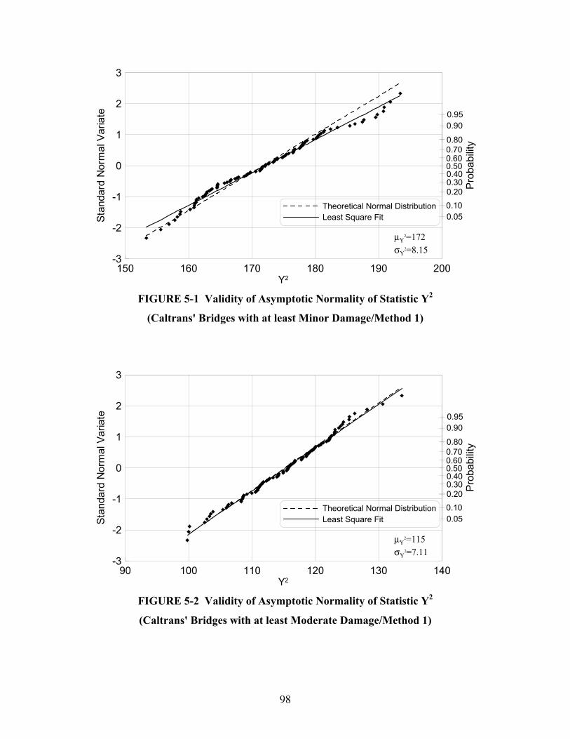
98
150 160 170 180 190 200Y2
-3
-2
-1
0
1
2
3
Stan
dard
Nor
mal
Var
iate
Prob
abilit
y
Theoretical Normal DistributionLeast Square Fit 0.05
0.100.200.30
0.50
0.700.80
0.60
0.40
0.900.95
µY2=172
σY2=8.15
FIGURE 5-1 Validity of Asymptotic Normality of Statistic Y2
(Caltrans' Bridges with at least Minor Damage/Method 1)
90 100 110 120 130 140Y2
-3
-2
-1
0
1
2
3
Stan
dard
Nor
mal
Var
iate
Prob
abilit
y
Theoretical Normal DistributionLeast Square Fit 0.05
0.100.200.30
0.50
0.700.80
0.60
0.40
0.900.95
µY2=115
σY2=7.11
FIGURE 5-2 Validity of Asymptotic Normality of Statistic Y2
(Caltrans' Bridges with at least Moderate Damage/Method 1)
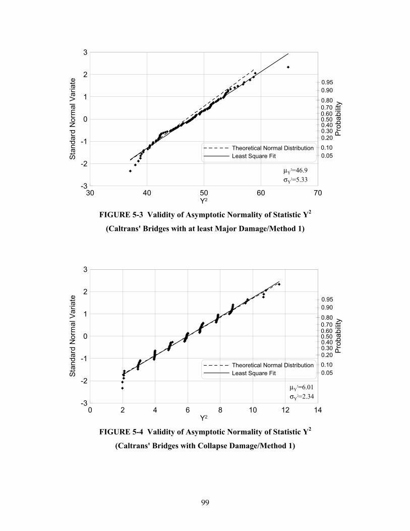
99
30 40 50 60 70Y2
-3
-2
-1
0
1
2
3
Stan
dard
Nor
mal
Var
iate
Prob
abilit
y
Theoretical Normal DistributionLeast Square Fit 0.05
0.100.200.30
0.50
0.700.80
0.60
0.40
0.900.95
µY2=46.9
σY2=5.33
FIGURE 5-3 Validity of Asymptotic Normality of Statistic Y2
(Caltrans' Bridges with at least Major Damage/Method 1)
0 2 4 6 8 10 12 14Y2
-3
-2
-1
0
1
2
3
Stan
dard
Nor
mal
Var
iate
Prob
abilit
y
Theoretical Normal DistributionLeast Square Fit 0.05
0.100.200.30
0.50
0.700.80
0.60
0.40
0.900.95
µY2=6.01
σY2=2.34
FIGURE 5-4 Validity of Asymptotic Normality of Statistic Y2
(Caltrans' Bridges with Collapse Damage/Method 1)
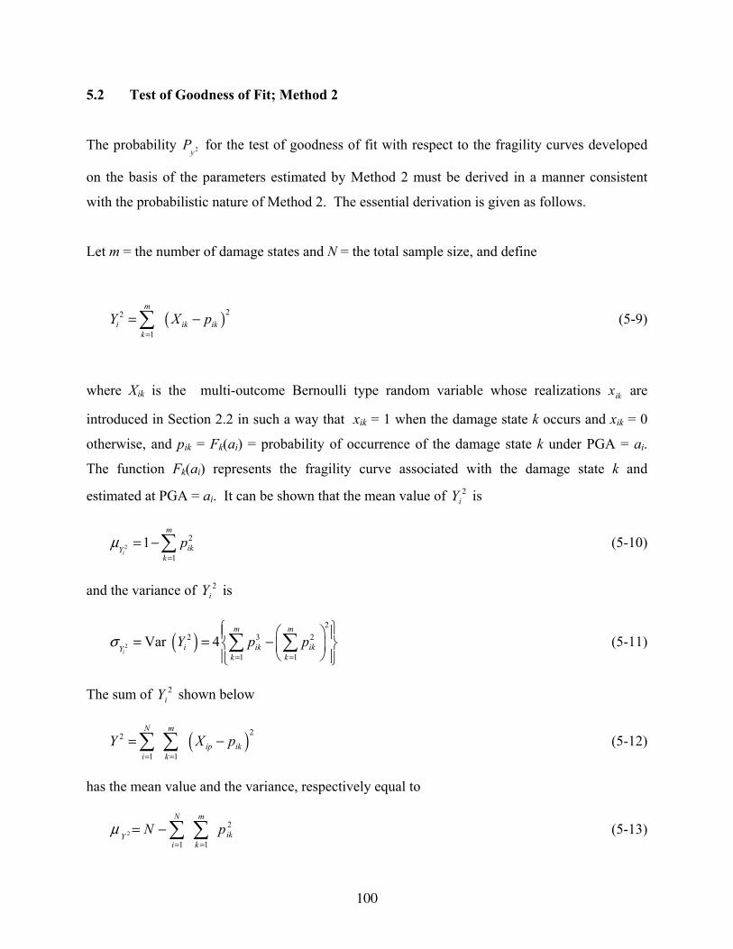
100
5.2 Test of Goodness of Fit; Method 2
The probability 2yP for the test of goodness of fit with respect to the fragility curves developed
on the basis of the parameters estimated by Method 2 must be derived in a manner consistent
with the probabilistic nature of Method 2. The essential derivation is given as follows.
Let m = the number of damage states and N = the total sample size, and define
( )22
1
m
i ik ikk
Y X p=
= −∑ (5-9)
where Xik is the multi-outcome Bernoulli type random variable whose realizations ikx are
introduced in Section 2.2 in such a way that xik = 1 when the damage state k occurs and xik = 0
otherwise, and pik = Fk(ai) = probability of occurrence of the damage state k under PGA = ai.
The function Fk(ai) represents the fragility curve associated with the damage state k and
estimated at PGA = ai. It can be shown that the mean value of 2iY is
22
11
i
m
ikYk
pµ=
= −∑ (5-10)
and the variance of 2iY is
( )2
22 3 2
1 1Var 4
i
m m
i ik ikYk k
Y p pσ= =
= = −
∑ ∑ (5-11)
The sum of 2iY shown below
( )22
1 1
N m
ip iki k
Y X p= =
= −∑ ∑ (5-12)
has the mean value and the variance, respectively equal to
2
112 ik
m
k
N
iY pN ∑∑
==−=µ (5-13)
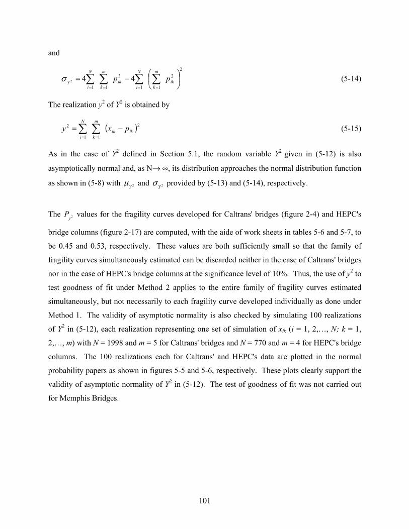
101
and
22
11
3
11442
−= ∑∑∑∑====
ik
m
k
N
iik
m
k
N
iY
ppσ (5-14)
The realization y2 of Y2 is obtained by
( )2
11
2ikik
m
k
N
ipxy −= ∑∑
==
(5-15)
As in the case of Y2 defined in Section 5.1, the random variable Y2 given in (5-12) is also
asymptotically normal and, as N→ ∞, its distribution approaches the normal distribution function
as shown in (5-8) with 2Yµ and 2Y
σ provided by (5-13) and (5-14), respectively.
The 2yP values for the fragility curves developed for Caltrans' bridges (figure 2-4) and HEPC's
bridge columns (figure 2-17) are computed, with the aide of work sheets in tables 5-6 and 5-7, to
be 0.45 and 0.53, respectively. These values are both sufficiently small so that the family of
fragility curves simultaneously estimated can be discarded neither in the case of Caltrans' bridges
nor in the case of HEPC's bridge columns at the significance level of 10%. Thus, the use of y2 to
test goodness of fit under Method 2 applies to the entire family of fragility curves estimated
simultaneously, but not necessarily to each fragility curve developed individually as done under
Method 1. The validity of asymptotic normality is also checked by simulating 100 realizations
of Y2 in (5-12), each realization representing one set of simulation of xik (i = 1, 2,…, N; k = 1,
2,…, m) with N = 1998 and m = 5 for Caltrans' bridges and N = 770 and m = 4 for HEPC's bridge
columns. The 100 realizations each for Caltrans' and HEPC's data are plotted in the normal
probability papers as shown in figures 5-5 and 5-6, respectively. These plots clearly support the
validity of asymptotic normality of Y2 in (5-12). The test of goodness of fit was not carried out
for Memphis Bridges.
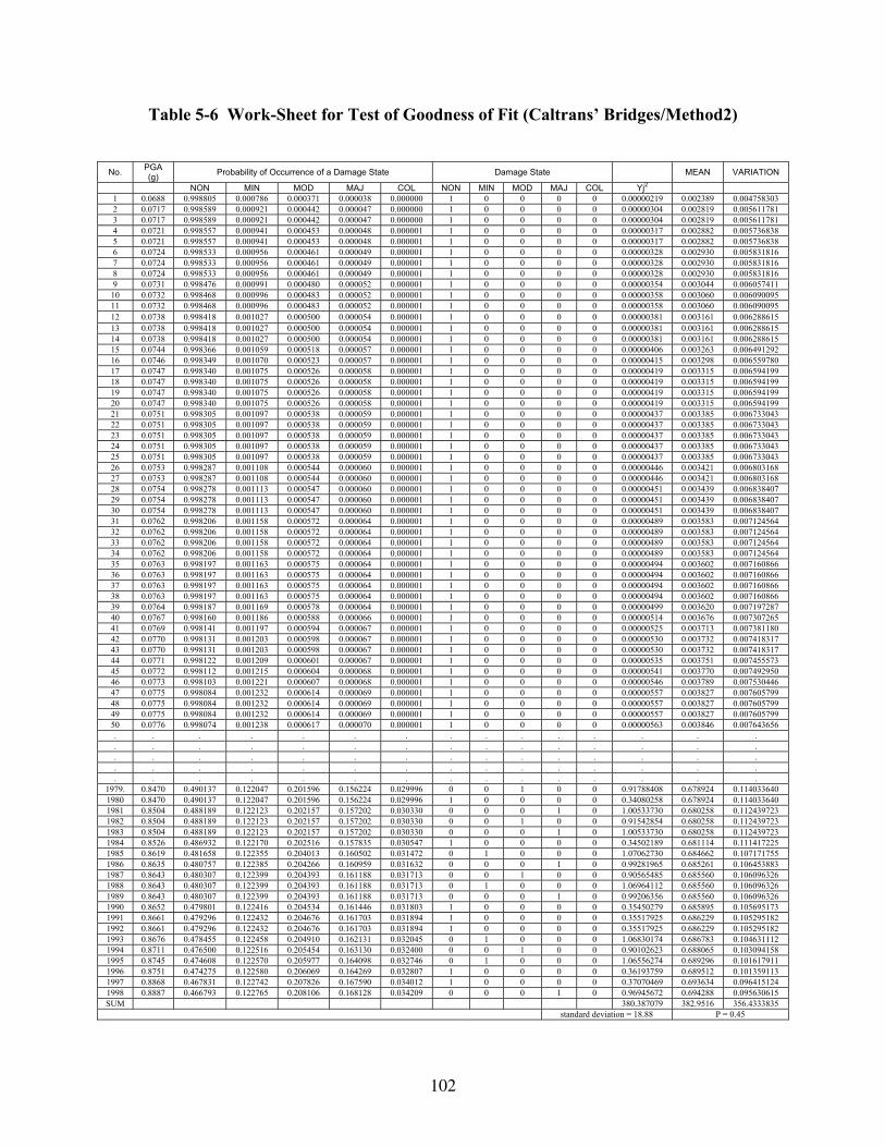
102
Table 5-6 Work-Sheet for Test of Goodness of Fit (Caltrans’ Bridges/Method2)
No. PGA (g) Probability of Occurrence of a Damage State Damage State MEAN VARIATION
NON MIN MOD MAJ COL NON MIN MOD MAJ COL Yj2 1 0.0688 0.998805 0.000786 0.000371 0.000038 0.000000 1 0 0 0 0 0.00000219 0.002389 0.004758303 2 0.0717 0.998589 0.000921 0.000442 0.000047 0.000000 1 0 0 0 0 0.00000304 0.002819 0.005611781 3 0.0717 0.998589 0.000921 0.000442 0.000047 0.000000 1 0 0 0 0 0.00000304 0.002819 0.005611781 4 0.0721 0.998557 0.000941 0.000453 0.000048 0.000001 1 0 0 0 0 0.00000317 0.002882 0.005736838 5 0.0721 0.998557 0.000941 0.000453 0.000048 0.000001 1 0 0 0 0 0.00000317 0.002882 0.005736838 6 0.0724 0.998533 0.000956 0.000461 0.000049 0.000001 1 0 0 0 0 0.00000328 0.002930 0.005831816 7 0.0724 0.998533 0.000956 0.000461 0.000049 0.000001 1 0 0 0 0 0.00000328 0.002930 0.005831816 8 0.0724 0.998533 0.000956 0.000461 0.000049 0.000001 1 0 0 0 0 0.00000328 0.002930 0.005831816 9 0.0731 0.998476 0.000991 0.000480 0.000052 0.000001 1 0 0 0 0 0.00000354 0.003044 0.006057411 10 0.0732 0.998468 0.000996 0.000483 0.000052 0.000001 1 0 0 0 0 0.00000358 0.003060 0.006090095 11 0.0732 0.998468 0.000996 0.000483 0.000052 0.000001 1 0 0 0 0 0.00000358 0.003060 0.006090095 12 0.0738 0.998418 0.001027 0.000500 0.000054 0.000001 1 0 0 0 0 0.00000381 0.003161 0.006288615 13 0.0738 0.998418 0.001027 0.000500 0.000054 0.000001 1 0 0 0 0 0.00000381 0.003161 0.006288615 14 0.0738 0.998418 0.001027 0.000500 0.000054 0.000001 1 0 0 0 0 0.00000381 0.003161 0.006288615 15 0.0744 0.998366 0.001059 0.000518 0.000057 0.000001 1 0 0 0 0 0.00000406 0.003263 0.006491292 16 0.0746 0.998349 0.001070 0.000523 0.000057 0.000001 1 0 0 0 0 0.00000415 0.003298 0.006559780 17 0.0747 0.998340 0.001075 0.000526 0.000058 0.000001 1 0 0 0 0 0.00000419 0.003315 0.006594199 18 0.0747 0.998340 0.001075 0.000526 0.000058 0.000001 1 0 0 0 0 0.00000419 0.003315 0.006594199 19 0.0747 0.998340 0.001075 0.000526 0.000058 0.000001 1 0 0 0 0 0.00000419 0.003315 0.006594199 20 0.0747 0.998340 0.001075 0.000526 0.000058 0.000001 1 0 0 0 0 0.00000419 0.003315 0.006594199 21 0.0751 0.998305 0.001097 0.000538 0.000059 0.000001 1 0 0 0 0 0.00000437 0.003385 0.006733043 22 0.0751 0.998305 0.001097 0.000538 0.000059 0.000001 1 0 0 0 0 0.00000437 0.003385 0.006733043 23 0.0751 0.998305 0.001097 0.000538 0.000059 0.000001 1 0 0 0 0 0.00000437 0.003385 0.006733043 24 0.0751 0.998305 0.001097 0.000538 0.000059 0.000001 1 0 0 0 0 0.00000437 0.003385 0.006733043 25 0.0751 0.998305 0.001097 0.000538 0.000059 0.000001 1 0 0 0 0 0.00000437 0.003385 0.006733043 26 0.0753 0.998287 0.001108 0.000544 0.000060 0.000001 1 0 0 0 0 0.00000446 0.003421 0.006803168 27 0.0753 0.998287 0.001108 0.000544 0.000060 0.000001 1 0 0 0 0 0.00000446 0.003421 0.006803168 28 0.0754 0.998278 0.001113 0.000547 0.000060 0.000001 1 0 0 0 0 0.00000451 0.003439 0.006838407 29 0.0754 0.998278 0.001113 0.000547 0.000060 0.000001 1 0 0 0 0 0.00000451 0.003439 0.006838407 30 0.0754 0.998278 0.001113 0.000547 0.000060 0.000001 1 0 0 0 0 0.00000451 0.003439 0.006838407 31 0.0762 0.998206 0.001158 0.000572 0.000064 0.000001 1 0 0 0 0 0.00000489 0.003583 0.007124564 32 0.0762 0.998206 0.001158 0.000572 0.000064 0.000001 1 0 0 0 0 0.00000489 0.003583 0.007124564 33 0.0762 0.998206 0.001158 0.000572 0.000064 0.000001 1 0 0 0 0 0.00000489 0.003583 0.007124564 34 0.0762 0.998206 0.001158 0.000572 0.000064 0.000001 1 0 0 0 0 0.00000489 0.003583 0.007124564 35 0.0763 0.998197 0.001163 0.000575 0.000064 0.000001 1 0 0 0 0 0.00000494 0.003602 0.007160866 36 0.0763 0.998197 0.001163 0.000575 0.000064 0.000001 1 0 0 0 0 0.00000494 0.003602 0.007160866 37 0.0763 0.998197 0.001163 0.000575 0.000064 0.000001 1 0 0 0 0 0.00000494 0.003602 0.007160866 38 0.0763 0.998197 0.001163 0.000575 0.000064 0.000001 1 0 0 0 0 0.00000494 0.003602 0.007160866 39 0.0764 0.998187 0.001169 0.000578 0.000064 0.000001 1 0 0 0 0 0.00000499 0.003620 0.007197287 40 0.0767 0.998160 0.001186 0.000588 0.000066 0.000001 1 0 0 0 0 0.00000514 0.003676 0.007307265 41 0.0769 0.998141 0.001197 0.000594 0.000067 0.000001 1 0 0 0 0 0.00000525 0.003713 0.007381180 42 0.0770 0.998131 0.001203 0.000598 0.000067 0.000001 1 0 0 0 0 0.00000530 0.003732 0.007418317 43 0.0770 0.998131 0.001203 0.000598 0.000067 0.000001 1 0 0 0 0 0.00000530 0.003732 0.007418317 44 0.0771 0.998122 0.001209 0.000601 0.000067 0.000001 1 0 0 0 0 0.00000535 0.003751 0.007455573 45 0.0772 0.998112 0.001215 0.000604 0.000068 0.000001 1 0 0 0 0 0.00000541 0.003770 0.007492950 46 0.0773 0.998103 0.001221 0.000607 0.000068 0.000001 1 0 0 0 0 0.00000546 0.003789 0.007530446 47 0.0775 0.998084 0.001232 0.000614 0.000069 0.000001 1 0 0 0 0 0.00000557 0.003827 0.007605799 48 0.0775 0.998084 0.001232 0.000614 0.000069 0.000001 1 0 0 0 0 0.00000557 0.003827 0.007605799 49 0.0775 0.998084 0.001232 0.000614 0.000069 0.000001 1 0 0 0 0 0.00000557 0.003827 0.007605799 50 0.0776 0.998074 0.001238 0.000617 0.000070 0.000001 1 0 0 0 0 0.00000563 0.003846 0.007643656 . . . . . . . . . . . . . . . . . . . . . . . . . . . . . . . . . . . . . . . . . . . . . . . . . . . . . . . . . . . . . . . . . . . . . . . . . . .
1979. 0.8470 0.490137 0.122047 0.201596 0.156224 0.029996 0 0 1 0 0 0.91788408 0.678924 0.114033640 1980 0.8470 0.490137 0.122047 0.201596 0.156224 0.029996 1 0 0 0 0 0.34080258 0.678924 0.114033640 1981 0.8504 0.488189 0.122123 0.202157 0.157202 0.030330 0 0 0 1 0 1.00533730 0.680258 0.112439723 1982 0.8504 0.488189 0.122123 0.202157 0.157202 0.030330 0 0 1 0 0 0.91542854 0.680258 0.112439723 1983 0.8504 0.488189 0.122123 0.202157 0.157202 0.030330 0 0 0 1 0 1.00533730 0.680258 0.112439723 1984 0.8526 0.486932 0.122170 0.202516 0.157835 0.030547 1 0 0 0 0 0.34502189 0.681114 0.111417225 1985 0.8619 0.481658 0.122355 0.204013 0.160502 0.031472 0 1 0 0 0 1.07062730 0.684662 0.107171755 1986 0.8635 0.480757 0.122385 0.204266 0.160959 0.031632 0 0 0 1 0 0.99281965 0.685261 0.106453883 1987 0.8643 0.480307 0.122399 0.204393 0.161188 0.031713 0 0 1 0 0 0.90565485 0.685560 0.106096326 1988 0.8643 0.480307 0.122399 0.204393 0.161188 0.031713 0 1 0 0 0 1.06964112 0.685560 0.106096326 1989 0.8643 0.480307 0.122399 0.204393 0.161188 0.031713 0 0 0 1 0 0.99206356 0.685560 0.106096326 1990 0.8652 0.479801 0.122416 0.204534 0.161446 0.031803 1 0 0 0 0 0.35450279 0.685895 0.105695173 1991 0.8661 0.479296 0.122432 0.204676 0.161703 0.031894 1 0 0 0 0 0.35517925 0.686229 0.105295182 1992 0.8661 0.479296 0.122432 0.204676 0.161703 0.031894 1 0 0 0 0 0.35517925 0.686229 0.105295182 1993 0.8676 0.478455 0.122458 0.204910 0.162131 0.032045 0 1 0 0 0 1.06830174 0.686783 0.104631112 1994 0.8711 0.476500 0.122516 0.205454 0.163130 0.032400 0 0 1 0 0 0.90102623 0.688065 0.103094158 1995 0.8745 0.474608 0.122570 0.205977 0.164098 0.032746 0 1 0 0 0 1.06556274 0.689296 0.101617911 1996 0.8751 0.474275 0.122580 0.206069 0.164269 0.032807 1 0 0 0 0 0.36193759 0.689512 0.101359113 1997 0.8868 0.467831 0.122742 0.207826 0.167590 0.034012 1 0 0 0 0 0.37070469 0.693634 0.096415124 1998 0.8887 0.466793 0.122765 0.208106 0.168128 0.034209 0 0 0 1 0 0.96945672 0.694288 0.095630615 SUM 380.387079 382.9516 356.4333835
standard deviation = 18.88 P = 0.45
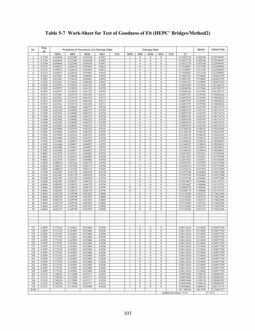
103
Table 5-7 Work-Sheet for Test of Goodness of Fit (HEPC’ Bridges/Method2)
No. PGA (g) Probability of Occurrence of a Damage State Damage State MEAN VARIATION
NON MIN MOD MAJ COL NON MIN MOD MAJ COL Yj2 1 0.3704 0.664664 0.222483 0.054106 0.0587 1 0 0 0 0.16832738 0.502344 0.229386997 2 0.3704 0.664664 0.222483 0.054106 0.0587 1 0 0 0 0.16832738 0.502344 0.229386997 3 0.3704 0.664664 0.222483 0.054106 0.0587 1 0 0 0 0.16832738 0.502344 0.229386997 4 0.3753 0.656073 0.226518 0.055863 0.0615 1 0 0 0 0.17650487 0.511349 0.222580992 5 0.3753 0.656073 0.226518 0.055863 0.0615 1 0 0 0 0.17650487 0.511349 0.222580992 6 0.3753 0.656073 0.226518 0.055863 0.0615 1 0 0 0 0.17650487 0.511349 0.222580992 7 0.3882 0.633681 0.236636 0.060483 0.0692 1 0 0 0 0.19863281 0.534005 0.204431070 8 0.3882 0.633681 0.236636 0.060483 0.0692 1 0 0 0 0.19863281 0.534005 0.204431070 9 0.3882 0.633681 0.236636 0.060483 0.0692 1 0 0 0 0.19863281 0.534005 0.204431070 10 0.3903 0.629975 0.238254 0.061253 0.0705 1 0 0 0 0.20240786 0.537642 0.201388735 11 0.3903 0.629975 0.238254 0.061253 0.0705 1 0 0 0 0.20240786 0.537642 0.201388735 12 0.3903 0.629975 0.238254 0.061253 0.0705 1 0 0 0 0.20240786 0.537642 0.201388735 13 0.3915 0.627861 0.239170 0.061693 0.0713 1 0 0 0 0.20457555 0.539702 0.199650224 14 0.3915 0.627861 0.239170 0.061693 0.0713 1 0 0 0 0.20457555 0.539702 0.199650224 15 0.3915 0.627861 0.239170 0.061693 0.0713 1 0 0 0 0.20457555 0.539702 0.199650224 16 0.3915 0.627861 0.239170 0.061693 0.0713 1 0 0 0 0.20457555 0.539702 0.199650224 17 0.3940 0.623642 0.240982 0.062572 0.0728 1 0 0 0 0.20893339 0.543783 0.196174719 18 0.3940 0.623642 0.240982 0.062572 0.0728 1 0 0 0 0.20893339 0.543783 0.196174719 19 0.3940 0.623642 0.240982 0.062572 0.0728 1 0 0 0 0.20893339 0.543783 0.196174719 20 0.3940 0.623642 0.240982 0.062572 0.0728 1 0 0 0 0.20893339 0.543783 0.196174719 21 0.3940 0.623642 0.240982 0.062572 0.0728 1 0 0 0 0.20893339 0.543783 0.196174719 22 0.3940 0.623642 0.240982 0.062572 0.0728 1 0 0 0 0.20893339 0.543783 0.196174719 23 0.3940 0.623642 0.240982 0.062572 0.0728 1 0 0 0 0.20893339 0.543783 0.196174719 24 0.3966 0.619084 0.242916 0.063523 0.0745 1 0 0 0 0.21368736 0.548145 0.192414385 25 0.3966 0.619084 0.242916 0.063523 0.0745 1 0 0 0 0.21368736 0.548145 0.192414385 26 0.3966 0.619084 0.242916 0.063523 0.0745 1 0 0 0 0.21368736 0.548145 0.192414385 27 0.3966 0.619084 0.242916 0.063523 0.0745 1 0 0 0 0.21368736 0.548145 0.192414385 28 0.3982 0.616460 0.244017 0.064072 0.0755 1 0 0 0 0.21644522 0.550634 0.190248435 29 0.3982 0.616460 0.244017 0.064072 0.0755 1 0 0 0 0.21644522 0.550634 0.190248435 30 0.3982 0.616460 0.244017 0.064072 0.0755 1 0 0 0 0.21644522 0.550634 0.190248435 31 0.3982 0.616460 0.244017 0.064072 0.0755 1 0 0 0 0.21644522 0.550634 0.190248435 32 0.4002 0.612970 0.245471 0.064802 0.0768 1 0 0 0 0.22013923 0.553921 0.187365696 33 0.4002 0.612970 0.245471 0.064802 0.0768 1 0 0 0 0.22013923 0.553921 0.187365696 34 0.4002 0.612970 0.245471 0.064802 0.0768 1 0 0 0 0.22013923 0.553921 0.187365696 35 0.4028 0.608619 0.247262 0.065714 0.0784 0 1 0 0 0.94749797 0.557979 0.183772499 36 0.4028 0.608619 0.247262 0.065714 0.0784 1 0 0 0 0.22478316 0.557979 0.183772499 37 0.4028 0.608619 0.247262 0.065714 0.0784 1 0 0 0 0.22478316 0.557979 0.183772499 38 0.3950 0.621887 0.241729 0.062938 0.0734 1 0 0 0 0.21075784 0.545468 0.194727680 39 0.3950 0.621887 0.241729 0.062938 0.0734 1 0 0 0 0.21075784 0.545468 0.194727680 40 0.3950 0.621887 0.241729 0.062938 0.0734 1 0 0 0 0.21075784 0.545468 0.194727680 41 0.4046 0.605495 0.248533 0.066370 0.0796 1 0 0 0 0.22814447 0.560866 0.181193743 42 0.4046 0.605495 0.248533 0.066370 0.0796 1 0 0 0 0.22814447 0.560866 0.181193743 43 0.4046 0.605495 0.248533 0.066370 0.0796 0 1 0 0 0.94206778 0.560866 0.181193743 44 0.4046 0.605495 0.248533 0.066370 0.0796 0 1 0 0 0.94206778 0.560866 0.181193743 45 0.4064 0.602378 0.249790 0.067025 0.0808 1 0 0 0 0.23152020 0.563723 0.178622996 46 0.4064 0.602378 0.249790 0.067025 0.0808 1 0 0 0 0.23152020 0.563723 0.178622996 47 0.4064 0.602378 0.249790 0.067025 0.0808 1 0 0 0 0.23152020 0.563723 0.178622996 48 0.4064 0.602378 0.249790 0.067025 0.0808 1 0 0 0 0.23152020 0.563723 0.178622996 49 0.4064 0.602378 0.249790 0.067025 0.0808 1 0 0 0 0.23152020 0.563723 0.178622996 50 0.4064 0.602378 0.249790 0.067025 0.0808 1 0 0 0 0.23152020 0.563723 0.178622996 . . . . . . . . . . . . . . . . . . . . . . . . . . . . . . . . . . . . . . . . . . . . . . . . . . . . . . . . . . . . . . . . .
751 0.3095 0.772192 0.165091 0.033086 0.0296 1 0 0 0 0.08112410 0.374492 0.294977550 752 0.3095 0.772192 0.165091 0.033086 0.0296 1 0 0 0 0.08112410 0.374492 0.294977550 753 0.3095 0.772192 0.165091 0.033086 0.0296 1 0 0 0 0.08112410 0.374492 0.294977550 754 0.3095 0.772192 0.165091 0.033086 0.0296 1 0 0 0 0.08112410 0.374492 0.294977550 755 0.3095 0.772192 0.165091 0.033086 0.0296 1 0 0 0 0.08112410 0.374492 0.294977550 756 0.3095 0.772192 0.165091 0.033086 0.0296 1 0 0 0 0.08112410 0.374492 0.294977550 757 0.3095 0.772192 0.165091 0.033086 0.0296 1 0 0 0 0.08112410 0.374492 0.294977550 758 0.3095 0.772192 0.165091 0.033086 0.0296 1 0 0 0 0.08112410 0.374492 0.294977550 759 0.3095 0.772192 0.165091 0.033086 0.0296 1 0 0 0 0.08112410 0.374492 0.294977550 760 0.3095 0.772192 0.165091 0.033086 0.0296 1 0 0 0 0.08112410 0.374492 0.294977550 761 0.3095 0.772192 0.165091 0.033086 0.0296 1 0 0 0 0.08112410 0.374492 0.294977550 762 0.3095 0.772192 0.165091 0.033086 0.0296 1 0 0 0 0.08112410 0.374492 0.294977550 763 0.3095 0.772192 0.165091 0.033086 0.0296 1 0 0 0 0.08112410 0.374492 0.294977550 764 0.3095 0.772192 0.165091 0.033086 0.0296 1 0 0 0 0.08112410 0.374492 0.294977550 765 0.3095 0.772192 0.165091 0.033086 0.0296 1 0 0 0 0.08112410 0.374492 0.294977550 766 0.3163 0.760238 0.172088 0.035317 0.0324 1 0 0 0 0.08939448 0.390130 0.290483593 767 0.3163 0.760238 0.172088 0.035317 0.0324 1 0 0 0 0.08939448 0.390130 0.290483593 768 0.3163 0.760238 0.172088 0.035317 0.0324 1 0 0 0 0.08939448 0.390130 0.290483593 769 0.3163 0.760238 0.172088 0.035317 0.0324 1 0 0 0 0.08939448 0.390130 0.290483593 770 0.3211 0.751810 0.176929 0.036908 0.0344 1 0 0 0 0.09544452 0.400935 0.286751119
SUM 457.700340 456.9798 87.28667327 standard deviation = 9.34 P = 0.53
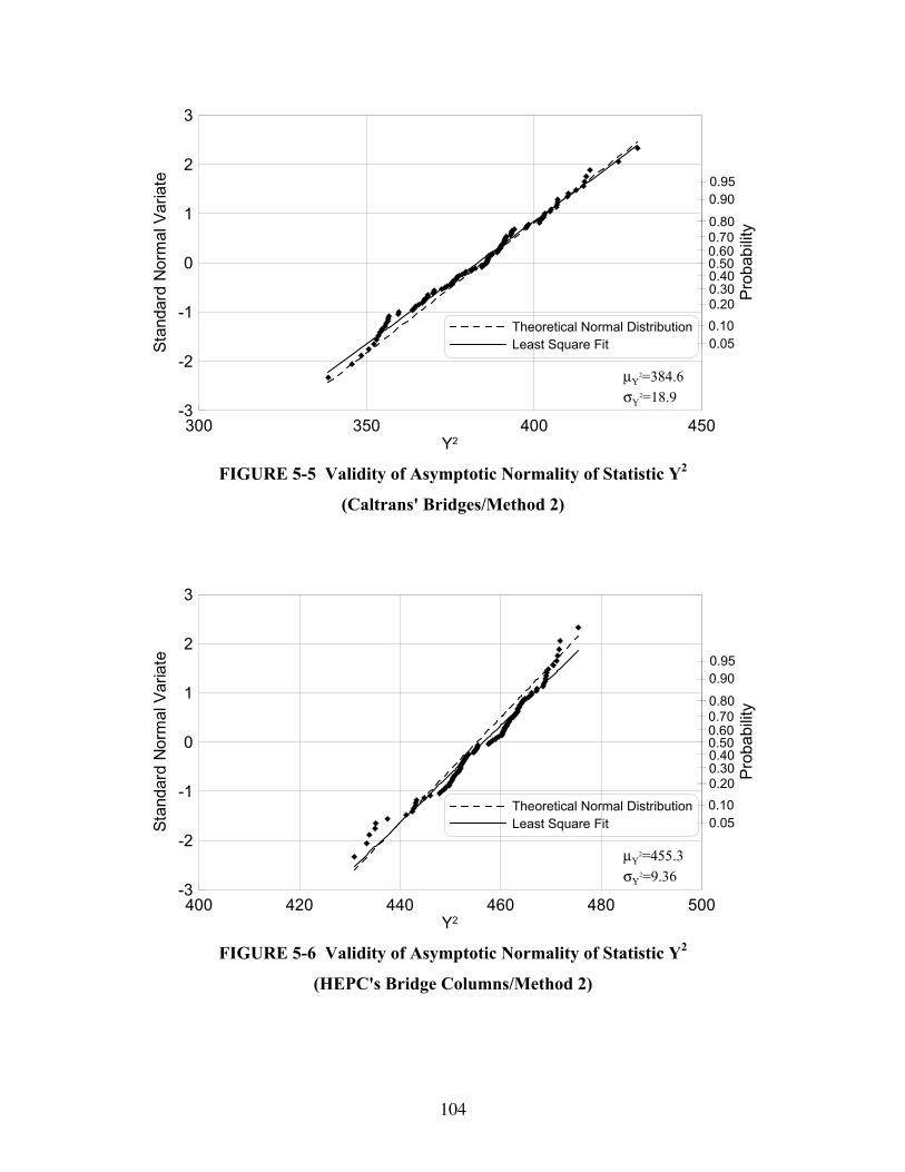
104
300 350 400 450Y2
-3
-2
-1
0
1
2
3
Stan
dard
Nor
mal
Var
iate
Prob
abilit
y
Theoretical Normal DistributionLeast Square Fit 0.05
0.100.200.30
0.50
0.700.80
0.60
0.40
0.900.95
µY2=384.6
σY2=18.9
FIGURE 5-5 Validity of Asymptotic Normality of Statistic Y2
(Caltrans' Bridges/Method 2)
400 420 440 460 480 500Y2
-3
-2
-1
0
1
2
3
Stan
dard
Nor
mal
Var
iate
Prob
abilit
y
Theoretical Normal DistributionLeast Square Fit 0.05
0.100.200.30
0.50
0.700.80
0.60
0.40
0.900.95
µY2=455.3
σY2=9.36
FIGURE 5-6 Validity of Asymptotic Normality of Statistic Y2
(HEPC's Bridge Columns/Method 2)
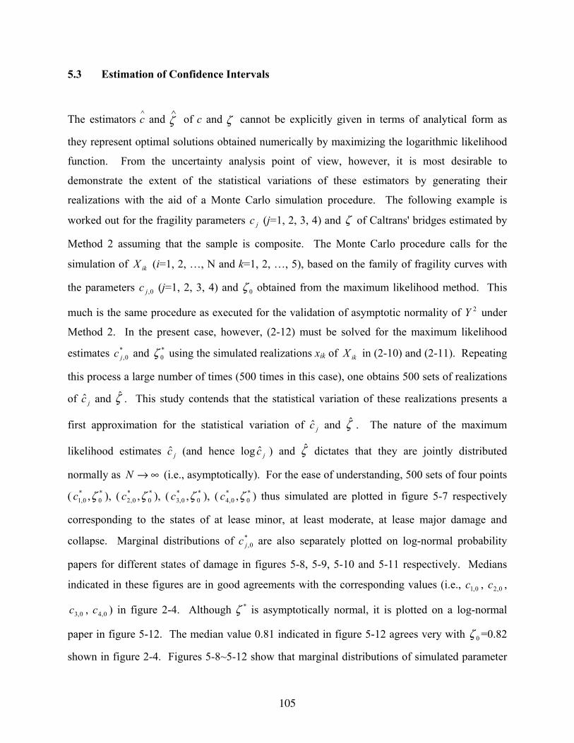
105
5.3 Estimation of Confidence Intervals
The estimators c∧ and
∧ζ of c and ζ cannot be explicitly given in terms of analytical form as
they represent optimal solutions obtained numerically by maximizing the logarithmic likelihood
function. From the uncertainty analysis point of view, however, it is most desirable to
demonstrate the extent of the statistical variations of these estimators by generating their
realizations with the aid of a Monte Carlo simulation procedure. The following example is
worked out for the fragility parameters jc (j=1, 2, 3, 4) and ζ of Caltrans' bridges estimated by
Method 2 assuming that the sample is composite. The Monte Carlo procedure calls for the
simulation of ikX (i=1, 2, …, N and k=1, 2, …, 5), based on the family of fragility curves with
the parameters 0,jc (j=1, 2, 3, 4) and 0ζ obtained from the maximum likelihood method. This
much is the same procedure as executed for the validation of asymptotic normality of 2Y under
Method 2. In the present case, however, (2-12) must be solved for the maximum likelihood
estimates *0,jc and *
0ζ using the simulated realizations xik of ikX in (2-10) and (2-11). Repeating
this process a large number of times (500 times in this case), one obtains 500 sets of realizations
of jc and ζ . This study contends that the statistical variation of these realizations presents a
first approximation for the statistical variation of jc and ζ . The nature of the maximum
likelihood estimates jc (and hence jclog ) and ζ dictates that they are jointly distributed
normally as ∞→N (i.e., asymptotically). For the ease of understanding, 500 sets of four points
( *0
*0,1 ,ζc ), ( *
0*
0,2 ,ζc ), ( *0
*0,3 ,ζc ), ( *
0*
0,4 ,ζc ) thus simulated are plotted in figure 5-7 respectively
corresponding to the states of at lease minor, at least moderate, at lease major damage and
collapse. Marginal distributions of *0,jc are also separately plotted on log-normal probability
papers for different states of damage in figures 5-8, 5-9, 5-10 and 5-11 respectively. Medians
indicated in these figures are in good agreements with the corresponding values (i.e., 0,1c , 0,2c ,
0,3c , 0,4c ) in figure 2-4. Although *ζ is asymptotically normal, it is plotted on a log-normal
paper in figure 5-12. The median value 0.81 indicated in figure 5-12 agrees very with 0ζ =0.82
shown in figure 2-4. Figures 5-8~5-12 show that marginal distributions of simulated parameter
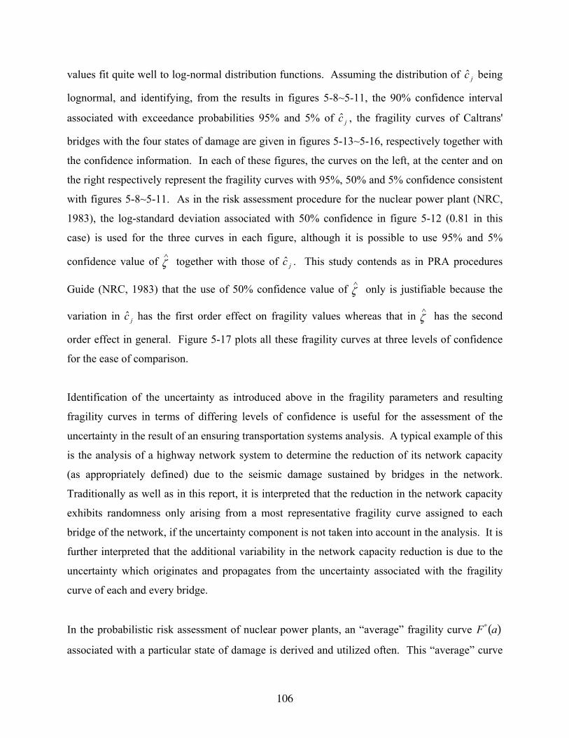
106
values fit quite well to log-normal distribution functions. Assuming the distribution of jc being
lognormal, and identifying, from the results in figures 5-8~5-11, the 90% confidence interval
associated with exceedance probabilities 95% and 5% of jc , the fragility curves of Caltrans'
bridges with the four states of damage are given in figures 5-13~5-16, respectively together with
the confidence information. In each of these figures, the curves on the left, at the center and on
the right respectively represent the fragility curves with 95%, 50% and 5% confidence consistent
with figures 5-8~5-11. As in the risk assessment procedure for the nuclear power plant (NRC,
1983), the log-standard deviation associated with 50% confidence in figure 5-12 (0.81 in this
case) is used for the three curves in each figure, although it is possible to use 95% and 5%
confidence value of ∧
ζ together with those of jc . This study contends as in PRA procedures
Guide (NRC, 1983) that the use of 50% confidence value of ∧
ζ only is justifiable because the
variation in jc has the first order effect on fragility values whereas that in ∧
ζ has the second
order effect in general. Figure 5-17 plots all these fragility curves at three levels of confidence
for the ease of comparison.
Identification of the uncertainty as introduced above in the fragility parameters and resulting
fragility curves in terms of differing levels of confidence is useful for the assessment of the
uncertainty in the result of an ensuring transportation systems analysis. A typical example of this
is the analysis of a highway network system to determine the reduction of its network capacity
(as appropriately defined) due to the seismic damage sustained by bridges in the network.
Traditionally as well as in this report, it is interpreted that the reduction in the network capacity
exhibits randomness only arising from a most representative fragility curve assigned to each
bridge of the network, if the uncertainty component is not taken into account in the analysis. It is
further interpreted that the additional variability in the network capacity reduction is due to the
uncertainty which originates and propagates from the uncertainty associated with the fragility
curve of each and every bridge.
In the probabilistic risk assessment of nuclear power plants, an “average” fragility curve F∗ a( )
associated with a particular state of damage is derived and utilized often. This “average” curve
107
is obtained by unconditionalizing ( ) ( )
Φ=
ζcacaF /ln| under the assumption that c is lognormally
distributed:
F∗ a( ) = F a | z( )z fc z( )dz (5-16)
where fc z( ) is the lognormal density function of c with median c~ and log-standard deviation ξc
as shown below.
( ) ( )
Φ=
c
cazcfζ
~/ln (5-17)
These median and log-standard deviation correspond to the respective values shown figures 5-
8~5-12. F∗ a( ) is not lognormal in general. However, in approximation, it may be and indeed
was used in practice as lognormal distribution in PRA Procedures Guide, (NRC, 1983).
0.1 1.0 10.0Median of PGA (g)
0.5
0.6
0.7
0.8
0.9
1
1.1
1.2
Log-
Stan
dard
Dev
iatio
n
Distribution of Median and Log-Standard Deviation
Minor Moderate CollapseMajor
FIGURE 5-7 Two-Dimensional Plot of 500 Sets of Simulated Realizations of Medians
( 1C , 2C , 3C , 4C ) and Log-Standard Deviations ξ
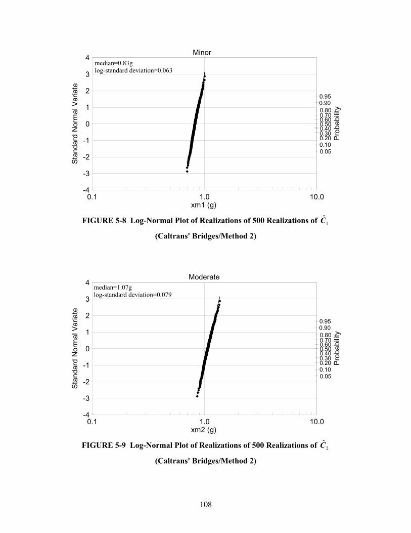
108
0.1 1.0 10.0xm1 (g)
-4
-3
-2
-1
0
1
2
3
4
Stan
dard
Nor
mal
Var
iate
Prob
abilit
y
0.050.100.200.300.500.700.800.600.40
0.900.95
median=0.83glog-standard deviation=0.063
Minor
FIGURE 5-8 Log-Normal Plot of Realizations of 500 Realizations of 1C
(Caltrans' Bridges/Method 2)
0.1 1.0 10.0xm2 (g)
-4
-3
-2
-1
0
1
2
3
4
Stan
dard
Nor
mal
Var
iate
Prob
abilit
y
0.050.100.200.300.500.700.800.600.40
0.900.95
median=1.07glog-standard deviation=0.079
Moderate
FIGURE 5-9 Log-Normal Plot of Realizations of 500 Realizations of 2C
(Caltrans' Bridges/Method 2)
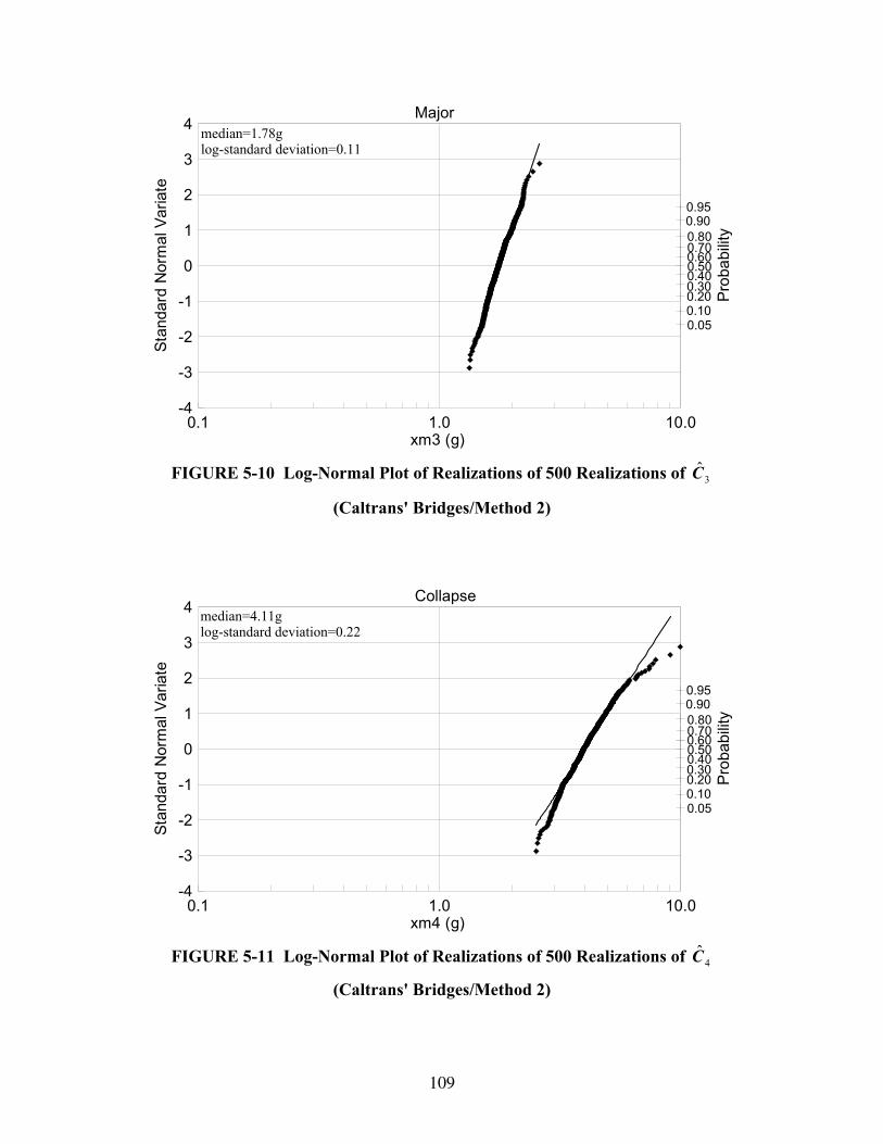
109
0.1 1.0 10.0xm3 (g)
-4
-3
-2
-1
0
1
2
3
4
Stan
dard
Nor
mal
Var
iate
Prob
abilit
y
0.050.100.200.300.500.700.800.600.40
0.900.95
median=1.78glog-standard deviation=0.11
Major
FIGURE 5-10 Log-Normal Plot of Realizations of 500 Realizations of 3C
(Caltrans' Bridges/Method 2)
0.1 1.0 10.0xm4 (g)
-4
-3
-2
-1
0
1
2
3
4
Stan
dard
Nor
mal
Var
iate
Prob
abilit
y
0.050.100.200.300.500.700.800.600.40
0.900.95
median=4.11glog-standard deviation=0.22
Collapse
FIGURE 5-11 Log-Normal Plot of Realizations of 500 Realizations of 4C
(Caltrans' Bridges/Method 2)
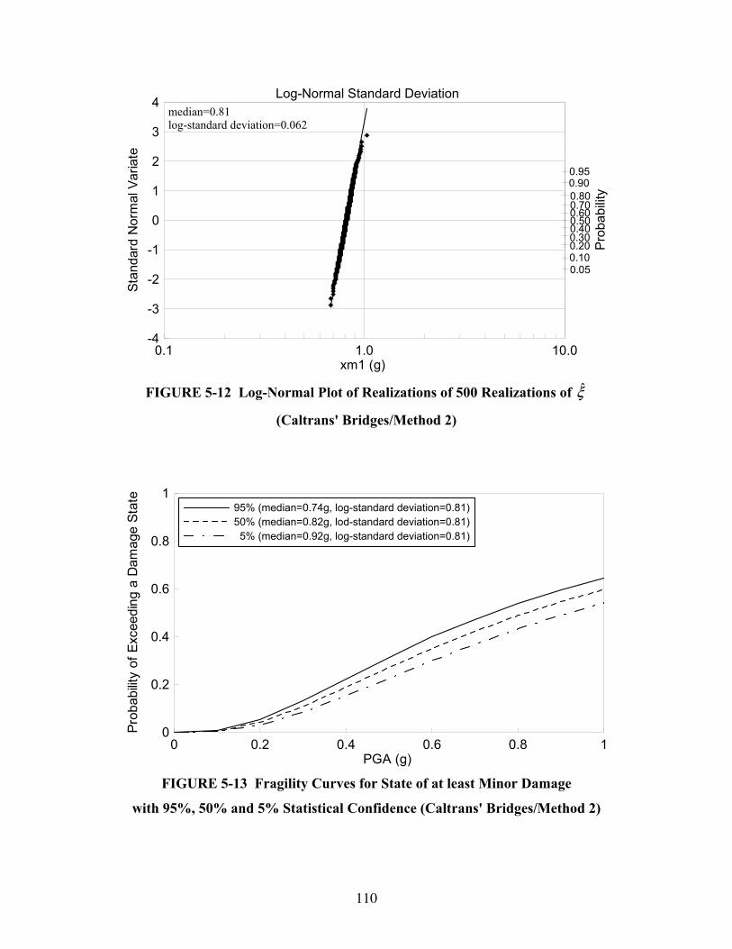
110
0.1 1.0 10.0xm1 (g)
-4
-3
-2
-1
0
1
2
3
4
Stan
dard
Nor
mal
Var
iate
Prob
abilit
y
0.050.100.200.300.500.700.800.600.40
0.900.95
median=0.81log-standard deviation=0.062
Log-Normal Standard Deviation
FIGURE 5-12 Log-Normal Plot of Realizations of 500 Realizations of ξ
(Caltrans' Bridges/Method 2)
0 0.2 0.4 0.6 0.8 1PGA (g)
0
0.2
0.4
0.6
0.8
1
Prob
abilit
y of
Exc
eedi
ng a
Dam
age
Stat
e
95% (median=0.74g, log-standard deviation=0.81)50% (median=0.82g, lod-standard deviation=0.81) 5% (median=0.92g, log-standard deviation=0.81)
FIGURE 5-13 Fragility Curves for State of at least Minor Damage
with 95%, 50% and 5% Statistical Confidence (Caltrans' Bridges/Method 2)

111
0 0.2 0.4 0.6 0.8 1PGA (g)
0
0.2
0.4
0.6
0.8
1
Prob
abilit
y of
Exc
eedi
ng a
Dam
age
Stat
e
95% (median=0.94g, log-standard deviation=0.81)50% (median=1.07g, lod-standard deviation=0.81) 5% (median=1.22g, log-standard deviation=0.81)
FIGURE 5-14 Fragility Curves for State of at least Moderate Damage
with 95%, 50% and 5% Statistical Confidence (Caltrans' Bridges/Method 2)
0 0.2 0.4 0.6 0.8 1PGA (g)
0
0.2
0.4
0.6
0.8
1
Prob
abilit
y of
Exc
eedi
ng a
Dam
age
Stat
e
95% (median=1.47g, log-standard deviation=0.81)50% (median=1.77g, lod-standard deviation=0.81) 5% (median=2.12g, log-standard deviation=0.81)
FIGURE 5-15 Fragility Curves for State of at least Major Damage
with 95%, 50% and 5% Statistical Confidence (Caltrans' Bridges/Method 2)
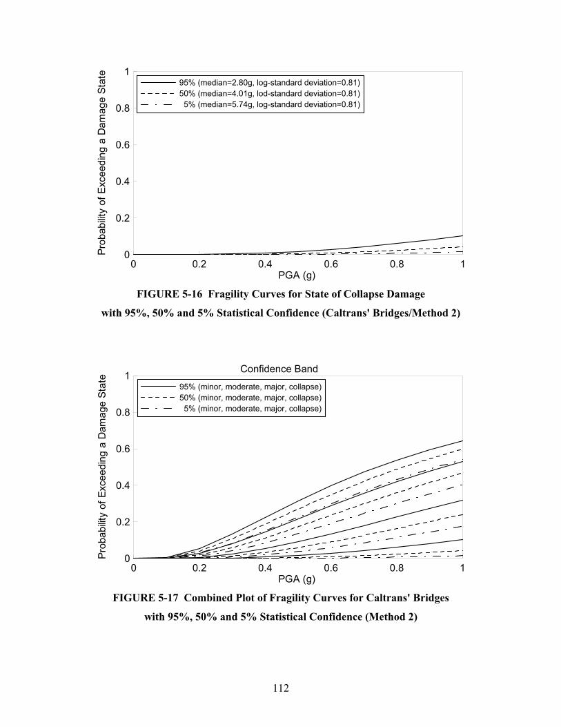
112
0 0.2 0.4 0.6 0.8 1PGA (g)
0
0.2
0.4
0.6
0.8
1
Prob
abilit
y of
Exc
eedi
ng a
Dam
age
Stat
e
95% (median=2.80g, log-standard deviation=0.81)50% (median=4.01g, lod-standard deviation=0.81) 5% (median=5.74g, log-standard deviation=0.81)
FIGURE 5-16 Fragility Curves for State of Collapse Damage
with 95%, 50% and 5% Statistical Confidence (Caltrans' Bridges/Method 2)
0 0.2 0.4 0.6 0.8 1PGA (g)
0
0.2
0.4
0.6
0.8
1
Prob
abilit
y of
Exc
eedi
ng a
Dam
age
Stat
e
95% (minor, moderate, major, collapse)50% (minor, moderate, major, collapse) 5% (minor, moderate, major, collapse)
Confidence Band
FIGURE 5-17 Combined Plot of Fragility Curves for Caltrans' Bridges
with 95%, 50% and 5% Statistical Confidence (Method 2)

113
5.4 Development of Combined Fragility Curves
Use of a fragility curve representing a family of bridges with similar structural attributes,
primarily categorized in specific structural types, expedites the process of urban earthquake
disaster estimation. A well-known example of such a categorization is found in ATC-13 (ATC,
1985). Bridges 1 and 2 in the Memphis area analyzed in an earlier section belong to a family of
bridges that can be categorized as precast prestressed continuous deck bridges with short to
medium length. This section demonstrates how combined fragility curves for a category of
bridges can be derived from individual fragility curves constructed for member bridges of the
category.
The fragility curves (associated with specific states of damage) analytically developed for
Bridges 1 and 2 in the Memphis area can be combined in the following fashion in order to
develop a combined fragility curve for a mixed bridge set population in which there are N1 and
N2 of Bridges 1 and 2, respectively. In this case, the combined fragility curve FC(a) is obtained
as
FC (a) = P1.F1(a) + P2.F2 (a) (5-18)
where Fi a( ) is the fragility curve for bridges i and
( )21 NNNP i
i += (5-19)
is the probability with which a bridge i will be chosen at random from the combined population.
The resulting fragility curve ( )aFC is shown in figure 5-18 together with the fragility curves that
are combined. It is noted that ( )aFC thus developed is no longer a lognormal distribution. The
corresponding density function is
( ) ( ) ( )afPafPafC 2211 += (5-20)
where fi a( ) is a lognormal density function associated with Fi(a). The expected value of
α = ln a for the combined distribution is given by
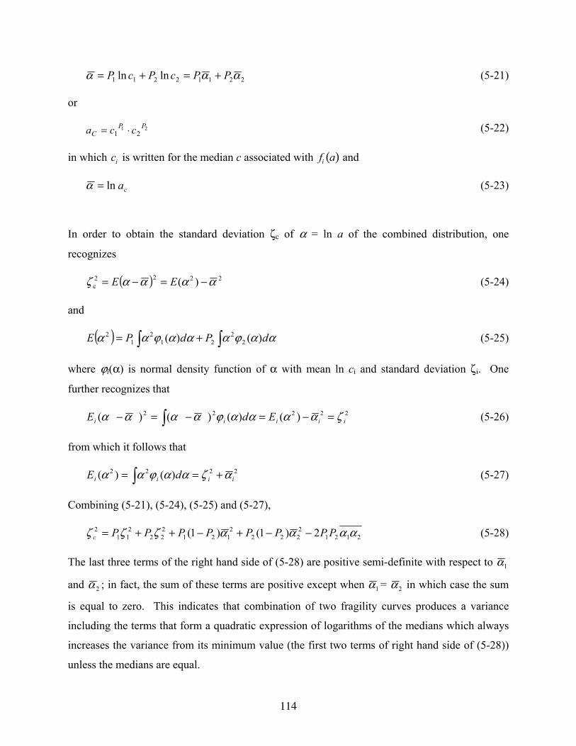
114
22112211 lnln ααα PPcPcP +=+= (5-21)
or
2121
PPC cca ⋅= (5-22)
in which ci is written for the median c associated with fi a( ) and
caln =α (5-23)
In order to obtain the standard deviation ζc of α = ln a of the combined distribution, one
recognizes
( ) 2222c )( ααααζ −=−= EE (5-24)
and
( ) ααϕαααϕαα dPdPE )()( 22
212
12 ∫ ∫+= (5-25)
where ϕi(α) is normal density function of α with mean ln ci and standard deviation ζi. One
further recognizes that
22222 )()()()( iiiii EdE ζααααϕαααα =−=−=− ∫ (5-26)
from which it follows that
2222 )()( iiii dE αζααϕαα +== ∫ (5-27)
Combining (5-21), (5-24), (5-25) and (5-27),
21212
2222
121222
211
2 2)1()1( ααααζζζ PPPPPPPPc −−+−++= (5-28)
The last three terms of the right hand side of (5-28) are positive semi-definite with respect to 1α
and 2α ; in fact, the sum of these terms are positive except when 1α = 2α in which case the sum
is equal to zero. This indicates that combination of two fragility curves produces a variance
including the terms that form a quadratic expression of logarithms of the medians which always
increases the variance from its minimum value (the first two terms of right hand side of (5-28))
unless the medians are equal.

115
(5-18)~(5-22) and (5-28) can all be easily generalized and take the following forms when the
population involves a large number (M) of bridges;
FC a( ) = PiFii=1
M
a( ) (5-29)
Pi =Ni
N (5-30)
where N = Nii =1
M
with Ni being the number of bridge i the population.
fC a( ) = Pii =1
M
fi a( ) (5-31)
i
M
iic Pa αα ∑
=
==1
ln (5-32)
1
M Pa c iC ii= ∏
=
(5-33)
and
AQAZP TTc +=2ζ (5-34)
where
[ ]MT PPPP 21 L= (5-35)
[ ]222
21 M
TZ ζζζ L= (5-36)
[ ]MTA ααα 21 L= (5-37)
and
Q =
−−−
−−−
)1(
)1(
21
12111
MMMM
M
PPPPPP
PPPPPP
L
M
M
L
(5-38)
116
The expression ATQ A is a quadratic form which is positive semi-definite being equal to zero
when 1α = 2α = … = Mα . Hence, the comment made above with respect to the increase of the
value of variance is also valid for M>2.
The combined fragility curve is not lognormal as explained earlier. It seems reasonable to
assume, however, that the combined curve is lognormal with the mean and variance estimated
respectively by (5-32) and (5-34). This approximation is expected to be particularly valid when
the bridges under consideration belong to a specific structural category as assumed here and are
designed under the same design codes.
The fragility curves developed for Caltrans' bridges in figure 2-3 and 2-4 and HEPC's bridge
columns in figure 2-16 and 2-17 are based on the total population, hypothetically homogeneous,
of their respective expressway bridges and bridge columns. These are referred to as composite
fragility curves in this study because they can be interpreted as composites of the combined
fragility curves just introduced, each being associated with a specific bridge category. The first
two moments of the composite fragility curves can also be derived from (a) the corresponding
first two moments of the combined fragility curves associated with the bridge categories in the
total population and (b) the relative size of sub-population of each bridge category to the size of
the total population.
The composite fragility curves are in general not lognormal either. Nevertheless, lognormal
assumption is used for composite curves as well in figures 2-3 and 2-4, and 2-16 and 2-17 for
analytical convenience and for the ease in which comparisons can be made with the fragility
curves developed for other structural and nonstructural systems many of which are traditionally
based on the lognormal assumption. It is noted that the lognormal assumption deployed in
constructing fragility curves throughout in this study indeed cannot be rejected according to the
result of the hypothesis testing involving the specific samples that were used. The inverse
analysis appears impossible that starts from the composite fragility curve to derive the combined
fragility curves and then the fragility curves of individual bridges.
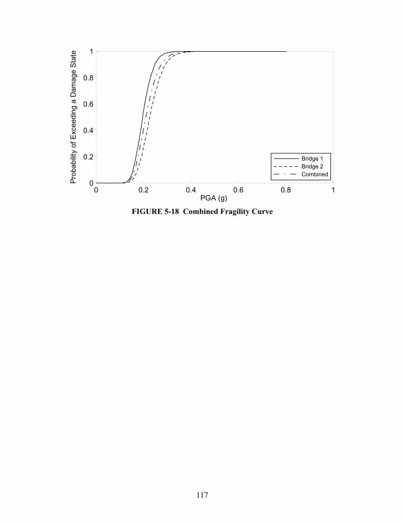
117
0 0.2 0.4 0.6 0.8 1PGA (g)
0
0.2
0.4
0.6
0.8
1
Prob
abilit
y of
Exc
eedi
ng a
Dam
age
Stat
e
Bridge 1Bridge 2Combined
FIGURE 5-18 Combined Fragility Curve

119
SECTION 6 SEISMIC RISK ASSESSMENT OF HIGHWAY NETWORKS
In this report, a seismic risk analysis is performed on the Los Angeles area expressway network.
For this purpose, the families of fragility curves for at least minor, at least moderate, at least
major and collapsed states of damage at the fourth level subgroupings, developed in figures 2-
24~2-36 are utilized. They are utilized to generate, in Monte Carlo simulation, the state of
damage for each and every Caltrans’ bridge in Los Angeles and Orange County (total number =
2,225) under postulated M = 7.1 Elysian Park earthquake. This means that if a bridge has a
combination of such attributes as multiple span (M), skew angle (θ2) between 0° and 20° and soil
condition C (c), then, the family of four fragility curves shown in figure 2-30 are to be used for
that bridge. If no fragility curve is given for a particular state of damage, for example, as in the
case of single span (see table 2-4(b)), a hypothetical fragility curve with median = 10g and log-
standard derivation = 0.78 as computed is assigned to ensure this state of damage not to occur in
simulation to be consistent with the empirical data. The five subgroups with such attribute
combinations as S/θ2/a, S/θ2/b, S/θ3/a, S/θ3/b and M/θ1/b produced no empirical damage data.
Assigned, in this case, to each state of damage for each of these subgroups is the same
hypothetical fragility curve with the median = 10g and log standard deviation = 0.5 for the same
reason. The simple procedure here is therefore to replace N/A in Median column by 10g and
N/A if found in Log. St. Dev. column by 0.5 to develop hypothetical fragility curves for those
attribute combinations for which table 2-4 does not provide complete information. This
procedure is theoretically unconservative and its effect on the result of the systems analysis as
undertaken in this section needs to be explored.
The state of damage thus simulated for each bridge is quantified using “bridge damage index,”
BDI, that is equal to 0.1, 0.3, 0.75 and 1.0 respectively for the minor, moderate, major and
collapsed state of damage. The state of link damage is then quantified by making use of “link
damage index”, LDI, which is computed for each link as the square root of the sum of the
squares of BDI values assigned to all bridges on the link under consideration. The LDI value is
then translated into link traffic flow capacity. In this study it is considered reasonable to assume
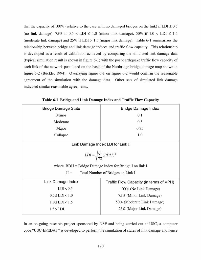
120
that the capacity of 100% (relative to the case with no damaged bridges on the link) if LDI ≤ 0.5
(no link damage), 75% if 0.5 < LDI ≤ 1.0 (minor link damage), 50% if 1.0 < LDI ≤ 1.5
(moderate link damage) and 25% if LDI > 1.5 (major link damage). Table 6-1 summarizes the
relationship between bridge and link damage indices and traffic flow capacity. This relationship
is developed as a result of calibration achieved by comparing the simulated link damage data
(typical simulation result is shown in figure 6-1) with the post-earthquake traffic flow capacity of
each link of the network postulated on the basis of the Northridge bridge damage map shown in
figure 6-2 (Buckle, 1994). Overlaying figure 6-1 on figure 6-2 would confirm the reasonable
agreement of the simulation with the damage data. Other sets of simulated link damage
indicated similar reasonable agreements.
Table 6-1 Bridge and Link Damage Index and Traffic Flow Capacity
Bridge Damage State Minor
Moderate
Major
Collapse
Bridge Damage Index 0.1
0.3
0.75
1.0
Link Damage Index LDI for Link I
∑=
=JI
JBDIJLDI
1
2)(
where BDIJ = Bridge Damage Index for Bridge J on link I
JI = Total Number of Bridges on Link I
Link Damage Index
LDI < 0.5
0.5 ≤ LDI < 1.0
1.0 ≤ LDI < 1.5
1.5 ≤ LDI
Traffic Flow Capacity (in terms of VPH) 100% (No Link Damage)
75% (Minor Link Damage)
50% (Moderate Link Damage)
25% (Major Link Damage)
In an on-going research project sponsored by NSF and being carried out at USC, a computer
code “USC-EPEDAT” is developed to perform the simulation of states of link damage and hence
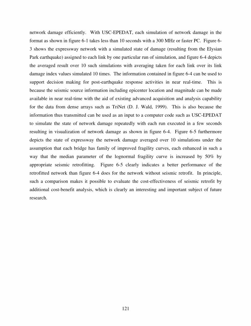
121
network damage efficiently. With USC-EPEDAT, each simulation of network damage in the
format as shown in figure 6-1 takes less than 10 seconds with a 300 MHz or faster PC. Figure 6-
3 shows the expressway network with a simulated state of damage (resulting from the Elysian
Park earthquake) assigned to each link by one particular run of simulation, and figure 6-4 depicts
the averaged result over 10 such simulations with averaging taken for each link over its link
damage index values simulated 10 times. The information contained in figure 6-4 can be used to
support decision making for post-earthquake response activities in near real-time. This is
because the seismic source information including epicenter location and magnitude can be made
available in near real-time with the aid of existing advanced acquisition and analysis capability
for the data from dense arrays such as TriNet (D. J. Wald, 1999). This is also because the
information thus transmitted can be used as an input to a computer code such as USC-EPEDAT
to simulate the state of network damage repeatedly with each run executed in a few seconds
resulting in visualization of network damage as shown in figure 6-4. Figure 6-5 furthermore
depicts the state of expressway the network damage averaged over 10 simulations under the
assumption that each bridge has family of improved fragility curves, each enhanced in such a
way that the median parameter of the lognormal fragility curve is increased by 50% by
appropriate seismic retrofitting. Figure 6-5 clearly indicates a better performance of the
retrofitted network than figure 6-4 does for the network without seismic retrofit. In principle,
such a comparison makes it possible to evaluate the cost-effectiveness of seismic retrofit by
additional cost-benefit analysis, which is clearly an interesting and important subject of future
research.
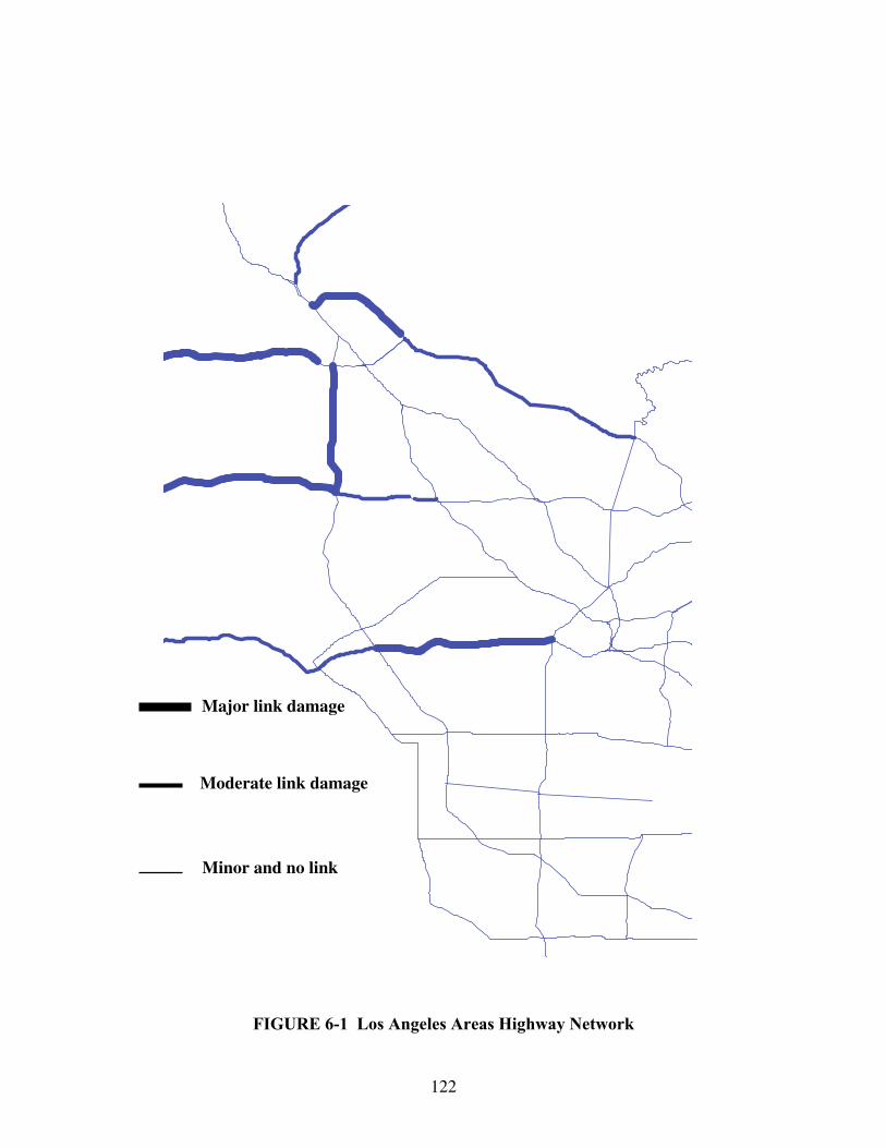
122
FIGURE 6-1 Los Angeles Areas Highway Network
Major link damage
Moderate link damage
Minor and no link
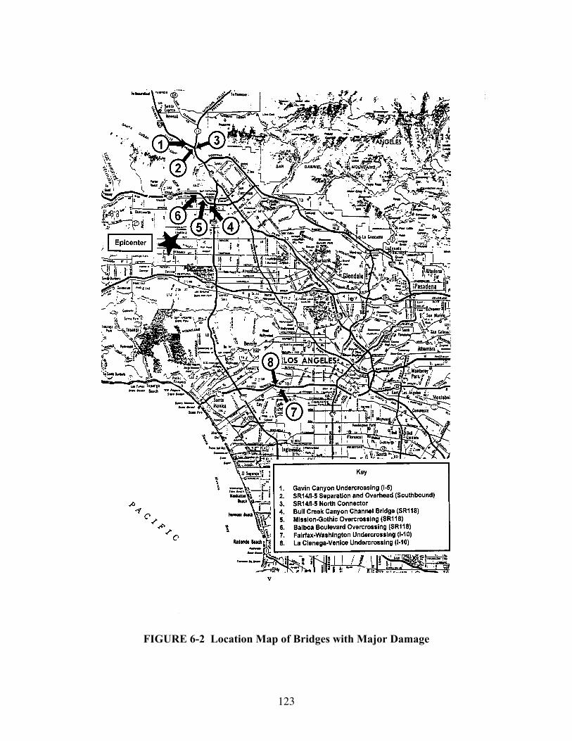
123
FIGURE 6-2 Location Map of Bridges with Major Damage
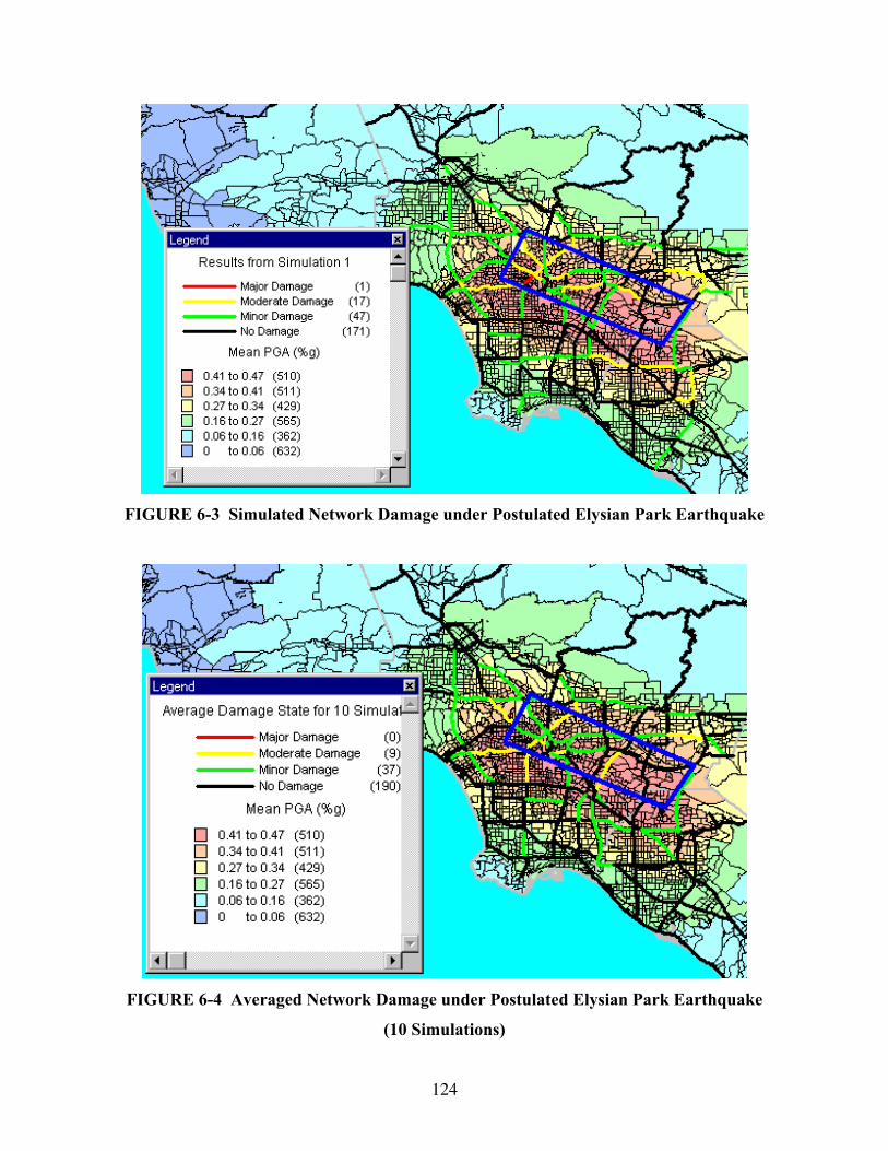
124
FIGURE 6-3 Simulated Network Damage under Postulated Elysian Park Earthquake
FIGURE 6-4 Averaged Network Damage under Postulated Elysian Park Earthquake
(10 Simulations)

125
FIGURE 6-5 Averaged Network Damage under Postulated Elysian Park Earthquake
(10 Simulations on retrofitted Network with Fragility Enhancement of 50%)

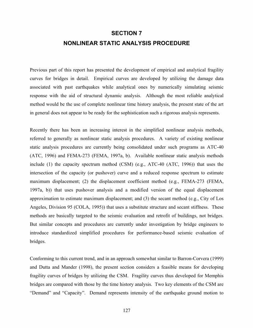
127
SECTION 7 NONLINEAR STATIC ANALYSIS PROCEDURE
Previous part of this report has presented the development of empirical and analytical fragility
curves for bridges in detail. Empirical curves are developed by utilizing the damage data
associated with past earthquakes while analytical ones by numerically simulating seismic
response with the aid of structural dynamic analysis. Although the most reliable analytical
method would be the use of complete nonlinear time history analysis, the present state of the art
in general does not appear to be ready for the sophistication such a rigorous analysis represents.
Recently there has been an increasing interest in the simplified nonlinear analysis methods,
referred to generally as nonlinear static analysis procedures. A variety of existing nonlinear
static analysis procedures are currently being consolidated under such programs as ATC-40
(ATC, 1996) and FEMA-273 (FEMA, 1997a, b). Available nonlinear static analysis methods
include (1) the capacity spectrum method (CSM) (e.g., ATC-40 (ATC, 1996)) that uses the
intersection of the capacity (or pushover) curve and a reduced response spectrum to estimate
maximum displacement; (2) the displacement coefficient method (e.g., FEMA-273 (FEMA,
1997a, b)) that uses pushover analysis and a modified version of the equal displacement
approximation to estimate maximum displacement; and (3) the secant method (e.g., City of Los
Angeles, Division 95 (COLA, 1995)) that uses a substitute structure and secant stiffness. These
methods are basically targeted to the seismic evaluation and retrofit of buildings, not bridges.
But similar concepts and procedures are currently under investigation by bridge engineers to
introduce standardized simplified procedures for performance-based seismic evaluation of
bridges.
Conforming to this current trend, and in an approach somewhat similar to Barron-Corvera (1999)
and Dutta and Mander (1998), the present section considers a feasible means for developing
fragility curves of bridges by utilizing the CSM. Fragility curves thus developed for Memphis
bridges are compared with those by the time history analysis. Two key elements of the CSM are
“Demand” and “Capacity”. Demand represents intensity of the earthquake ground motion to
128
which bridges are subjected, while capacity represents the bridges’ ability to resist the seismic
demand. CSM requires determination of three primary elements: capacity spectrum, demand
spectrum and performance point. Each of these elements utilized in this report basically
conforms to ATC-40 (ATC, 1996) and briefly discussed below for better understanding.
7.1 CSM: Capacity Spectrum
In order to determine a capacity beyond the elastic limits, the pushover analysis is performed.
The standard way to plot the force-displacement curve is by tracking the total shear force at
column bottoms as a function of displacement of the superstructure.
The lateral forces are applied in proportion to the fundamental mode shape as shown in (7-1)
below where iF is the lateral force on node ),,2,1( Nii L= , iw dead weight assigned to node i ,
iφ amplitude of the fundamental mode at node i , V the base shear and N the number of nodes.
VwwFN
iiiiii
= ∑=1
φφ (7-1)
The corresponding natural period at any point on the capacity curve can be calculated by using of
(7-2) below where T is the period of the fundamental mode, iδ lateral displacement at node i
due to lateral forces, g acceleration due to gravity.
= ∑∑==
N
iii
N
iii FgwT
11
22 δδπ (7-2)
To use the CSM, it is necessary to convert the capacity curve to capacity spectrum. The capacity
curve expresses overall shear force on all supports as a function of the horizontal displacement of
the superstructure, whereas the capacity spectrum represents the capacity curve in the ADRS
(Acceleration-Displacement Response Spectra) format. The spectral acceleration aS and the
spectral displacement dS can be calculated using modal parameters at any level of load
magnitude as follows:
129
αWV
S a = (7-3)
pl
pl
girder
girderd PFPF
Sφ
θφ
≅∆
= (7-4)
where W is overall dead weight of bridge, girder∆ horizontal displacement of girder, plθ rotation
of plastic hinge, girderφ and plφ amplitudes of the fundamental mode at girder and plastic hinge,
respectively, PF and α modal participation factor and modal mass coefficient of the
fundamental mode defined as follows:
( )
( )
=
∑
∑
=
=N
iii
N
iii
gw
gwPF
1
2
1
φ
φ (7-5)
( )
( )
=
∑∑
∑
==
=
N
iii
N
ii
N
iii
gwgw
gw
1
2
1
2
1
φ
φα (7-6)
The spectral displacement dS can be obtained from any displacement component of the structure
as shown in (7-4). For bridge structures, the horizontal displacement of girder is a most critical
displacement component for developing the capacity curve. However, the rotation of plastic
hinge is more conveniently used to develop the capacity curve when the rotational ductility
factor of plastic hinges at column bottoms is used to represent the damage states as in the present
study. Figure 7-1 shows the capacity spectra developed for the 10 sample bridges introduced in
Section 3.
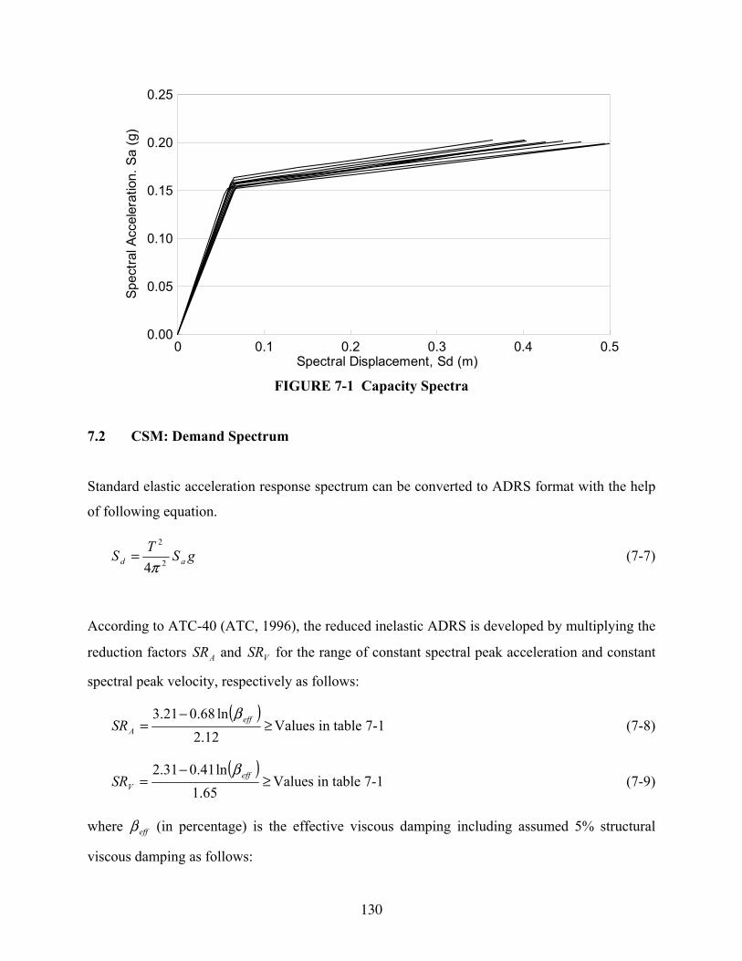
130
0 0.1 0.2 0.3 0.4 0.5Spectral Displacement, Sd (m)
0.00
0.05
0.10
0.15
0.20
0.25
Spec
tral A
ccel
erat
ion.
Sa
(g)
FIGURE 7-1 Capacity Spectra
7.2 CSM: Demand Spectrum
Standard elastic acceleration response spectrum can be converted to ADRS format with the help
of following equation.
gSTS ad 2
2
4π= (7-7)
According to ATC-40 (ATC, 1996), the reduced inelastic ADRS is developed by multiplying the
reduction factors ASR and VSR for the range of constant spectral peak acceleration and constant
spectral peak velocity, respectively as follows:
( )≥
−=
12.2ln68.021.3 eff
ASRβ
Values in table 7-1 (7-8)
( )≥
−=
65.1ln41.031.2 eff
VSRβ
Values in table 7-1 (7-9)
where effβ (in percentage) is the effective viscous damping including assumed 5% structural
viscous damping as follows:
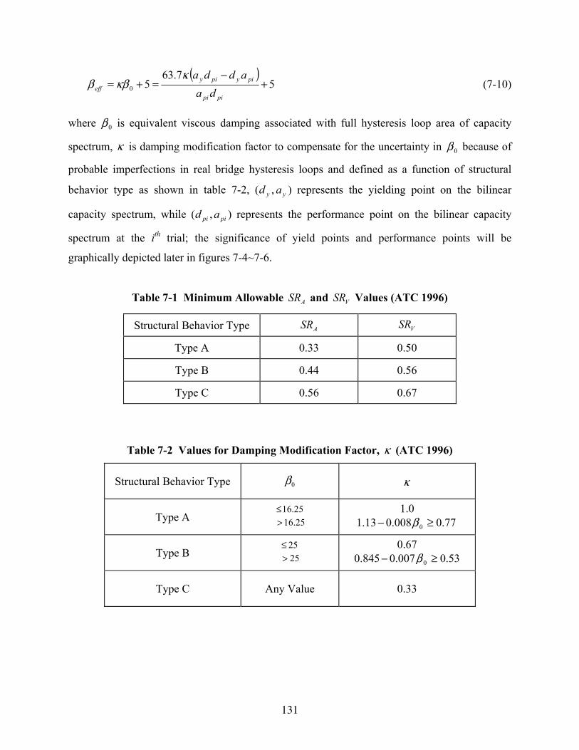
131
( )5
7.6350 +
−=+=
pipi
piypiyeff da
addaκκββ (7-10)
where 0β is equivalent viscous damping associated with full hysteresis loop area of capacity
spectrum, κ is damping modification factor to compensate for the uncertainty in 0β because of
probable imperfections in real bridge hysteresis loops and defined as a function of structural
behavior type as shown in table 7-2, ),( yy ad represents the yielding point on the bilinear
capacity spectrum, while ),( pipi ad represents the performance point on the bilinear capacity
spectrum at the ith trial; the significance of yield points and performance points will be
graphically depicted later in figures 7-4~7-6.
Table 7-1 Minimum Allowable ASR and VSR Values (ATC 1996)
Structural Behavior Type ASR VSR
Type A 0.33 0.50
Type B 0.44 0.56
Type C 0.56 0.67
Table 7-2 Values for Damping Modification Factor, κ (ATC 1996)
Structural Behavior Type 0β κ
Type A 25.16≤ 25.16>
1.0 77.0008.013.1 0 ≥− β
Type B 25≤ 25>
0.67 53.0007.0845.0 0 ≥− β
Type C Any Value 0.33
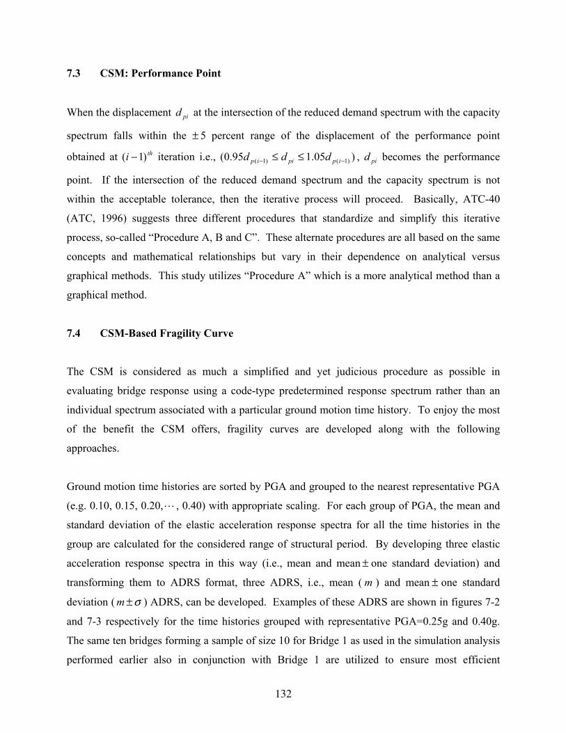
132
7.3 CSM: Performance Point
When the displacement pid at the intersection of the reduced demand spectrum with the capacity
spectrum falls within the 5± percent range of the displacement of the performance point
obtained at thi )1( − iteration i.e., )05.195.0( )1()1( −− ≤≤ ippiip ddd , pid becomes the performance
point. If the intersection of the reduced demand spectrum and the capacity spectrum is not
within the acceptable tolerance, then the iterative process will proceed. Basically, ATC-40
(ATC, 1996) suggests three different procedures that standardize and simplify this iterative
process, so-called “Procedure A, B and C”. These alternate procedures are all based on the same
concepts and mathematical relationships but vary in their dependence on analytical versus
graphical methods. This study utilizes “Procedure A” which is a more analytical method than a
graphical method.
7.4 CSM-Based Fragility Curve
The CSM is considered as much a simplified and yet judicious procedure as possible in
evaluating bridge response using a code-type predetermined response spectrum rather than an
individual spectrum associated with a particular ground motion time history. To enjoy the most
of the benefit the CSM offers, fragility curves are developed along with the following
approaches.
Ground motion time histories are sorted by PGA and grouped to the nearest representative PGA
(e.g. 0.10, 0.15, 0.20,L , 0.40) with appropriate scaling. For each group of PGA, the mean and
standard deviation of the elastic acceleration response spectra for all the time histories in the
group are calculated for the considered range of structural period. By developing three elastic
acceleration response spectra in this way (i.e., mean and mean ± one standard deviation) and
transforming them to ADRS format, three ADRS, i.e., mean ( m ) and mean ± one standard
deviation ( σ±m ) ADRS, can be developed. Examples of these ADRS are shown in figures 7-2
and 7-3 respectively for the time histories grouped with representative PGA=0.25g and 0.40g.
The same ten bridges forming a sample of size 10 for Bridge 1 as used in the simulation analysis
performed earlier also in conjunction with Bridge 1 are utilized to ensure most efficient
133
comparison. These bridges are referred to as sample bridge 1, 2,L , 10 to be distinguished from
Bridge 1. Then a capacity spectrum for each sample bridge is one by one constructed and drawn
on the same coordinates. The three performance points for each of the capacity spectrum are
determined as its intersections with m and σ±m ADRS reduced properly using the reduction
factors introduced in (7-8) and (7-9). These three spectral displacements are defined as )(aSd
and )()( aaS dd σ± , and shown in figures 7-4~7-6 for PGA=0.25g. Indeed, they are functions of
a (PGA) since the three ADRS on which they depend are developed on the time histories sorted
and grouped by PGA.
Assuming the two-parameter lognormal distribution for the spectral displacement )(aSd , the
parameters can be obtained from following equations.
]2)}({exp[)()( 2aacaS d ζ= (7-11)
[ ]1))}(exp({)}({)}({ 222 −= aaSa dd ζσ (7-12)
The limit displacement ld which is defined as the spectral displacement )(aSd for the specified
state of damage can be expressed by (7-13) with the aid of (7-4).
ydamagepl
damage
ypl
ypll PF
DemandDuctilityPF
dθφθφ
θθ)(
)(== (7-13)
where ( )damageX denotes the value of X at the specified state of damage and yθ is the yielding
rotation of the plastic hinge. To be consistent with the analytical fragility curves for Bridge 1 in
the Memphis area developed earlier, the state of damage described by ductility demand being
larger than 1.0 or 2.0 simultaneously existing for all the bridge columns represent the minor or
major states of damage. Hence, damageDemandDuctility )( in (7-13) should be 1.0 for the state of
minor damage and 2.0 for the state of major damage. It should be addressed here that the limit
displacement ld for each sample bridge is slightly different with each other for even the same
state of damage because damageplPF )( φ is not identical for each sample bridge. The probability
that sample bridge j will have a state of damage exceeding ld is given by
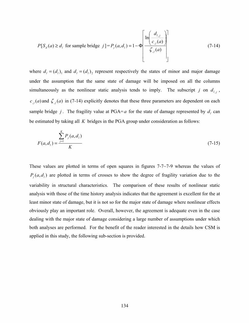
134
ld daSP ≥)([ for sample bridge ]j =
Φ−=)(
)(ln
1),(,
,
,
a
acd
daPj
j
jl
lj ζ (7-14)
where 1)( ll dd = and 2)( ll dd = represent respectively the states of minor and major damage
under the assumption that the same state of damage will be imposed on all the columns
simultaneously as the nonlinear static analysis tends to imply. The subscript j on jld , ,
)(, ac j and )(, ajζ in (7-14) explicitly denotes that these three parameters are dependent on each
sample bridge j . The fragility value at PGA= a for the state of damage represented by ld can
be estimated by taking all K bridges in the PGA group under consideration as follows:
K
daPdaF
K
jlj
l
∑== 1
),(),( (7-15)
These values are plotted in terms of open squares in figures 7-7~7-9 whereas the values of
),( lj daP are plotted in terms of crosses to show the degree of fragility variation due to the
variability in structural characteristics. The comparison of these results of nonlinear static
analysis with those of the time history analysis indicates that the agreement is excellent for the at
least minor state of damage, but it is not so for the major state of damage where nonlinear effects
obviously play an important role. Overall, however, the agreement is adequate even in the case
dealing with the major state of damage considering a large number of assumptions under which
both analyses are performed. For the benefit of the reader interested in the details how CSM is
applied in this study, the following sub-section is provided.
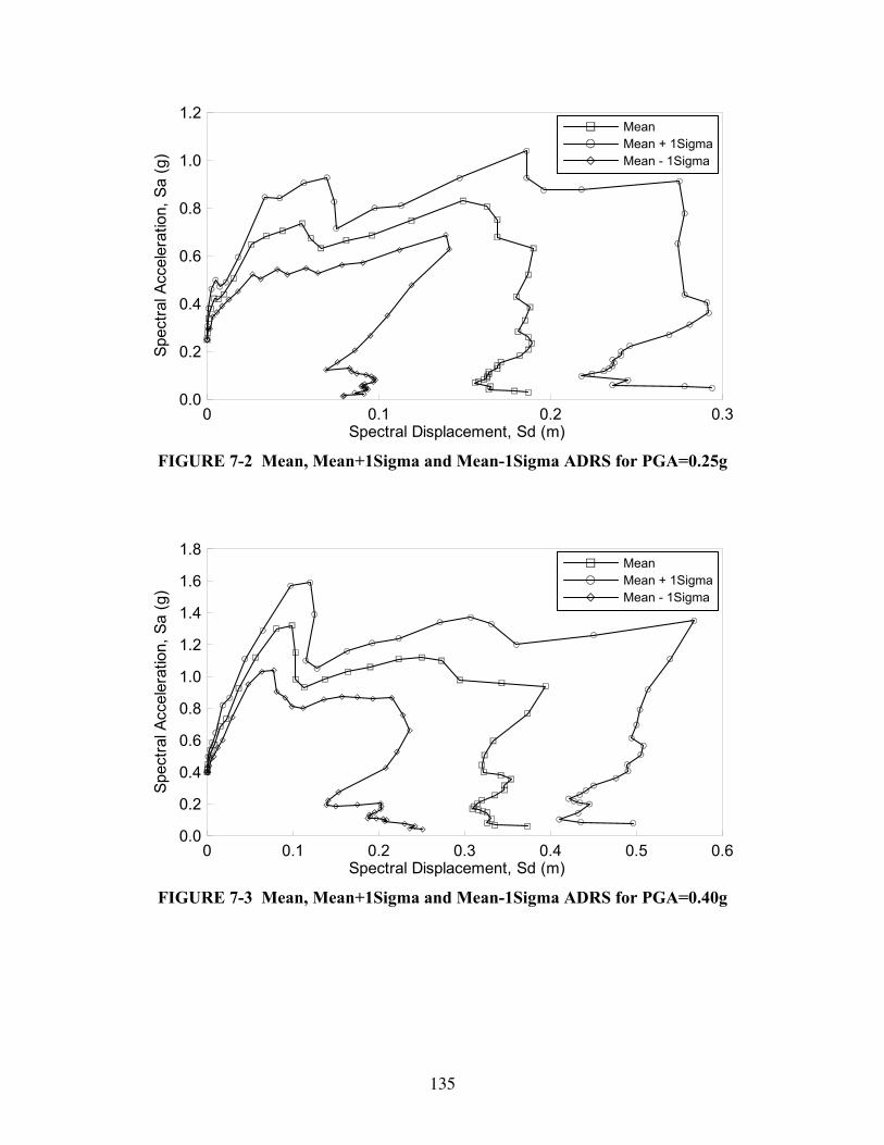
135
0 0.1 0.2 0.3Spectral Displacement, Sd (m)
0.0
0.2
0.4
0.6
0.8
1.0
1.2
Spec
tral A
ccel
erat
ion,
Sa
(g)
MeanMean + 1SigmaMean - 1Sigma
FIGURE 7-2 Mean, Mean+1Sigma and Mean-1Sigma ADRS for PGA=0.25g
0 0.1 0.2 0.3 0.4 0.5 0.6Spectral Displacement, Sd (m)
0.0
0.2
0.4
0.6
0.8
1.0
1.2
1.4
1.6
1.8
Spec
tral A
ccel
erat
ion,
Sa
(g)
MeanMean + 1SigmaMean - 1Sigma
FIGURE 7-3 Mean, Mean+1Sigma and Mean-1Sigma ADRS for PGA=0.40g
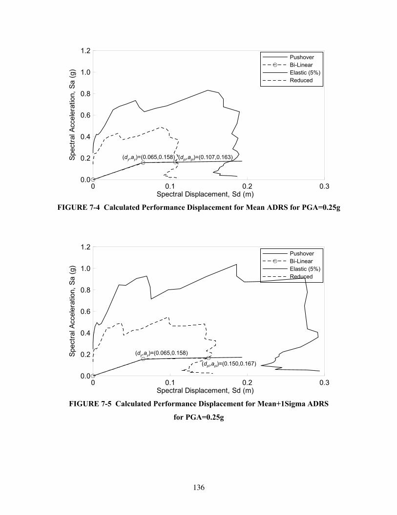
136
0 0.1 0.2 0.3Spectral Displacement, Sd (m)
0.0
0.2
0.4
0.6
0.8
1.0
1.2
Spec
tral A
ccel
erat
ion,
Sa
(g)
PushoverBi-LinearElastic (5%)Reduced
(dy,ay)=(0.065,0.158) (dpi,api)=(0.107,0.163)
FIGURE 7-4 Calculated Performance Displacement for Mean ADRS for PGA=0.25g
0 0.1 0.2 0.3Spectral Displacement, Sd (m)
0.0
0.2
0.4
0.6
0.8
1.0
1.2
Spec
tral A
ccel
erat
ion,
Sa
(g)
PushoverBi-LinearElastic (5%)Reduced
(dy,ay)=(0.065,0.158)
(dpi,api)=(0.150,0.167)
FIGURE 7-5 Calculated Performance Displacement for Mean+1Sigma ADRS
for PGA=0.25g
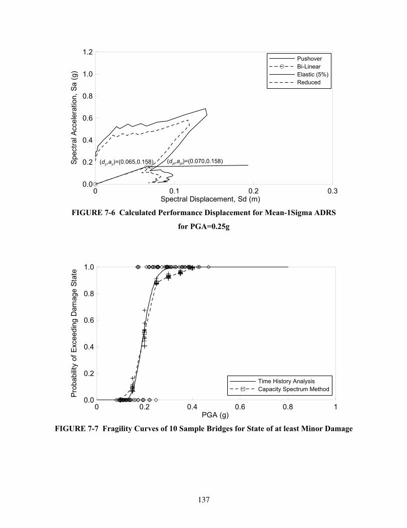
137
0 0.1 0.2 0.3Spectral Displacement, Sd (m)
0.0
0.2
0.4
0.6
0.8
1.0
1.2
Spec
tral A
ccel
erat
ion,
Sa
(g)
PushoverBi-LinearElastic (5%)Reduced
(dy,ay)=(0.065,0.158) (dpi,api)=(0.070,0.158)
FIGURE 7-6 Calculated Performance Displacement for Mean-1Sigma ADRS
for PGA=0.25g
0 0.2 0.4 0.6 0.8 1PGA (g)
0.0
0.2
0.4
0.6
0.8
1.0
Prob
abilit
y of
Exc
eedi
ng D
amag
e St
ate
Time History AnalysisCapacity Spectrum Method
FIGURE 7-7 Fragility Curves of 10 Sample Bridges for State of at least Minor Damage
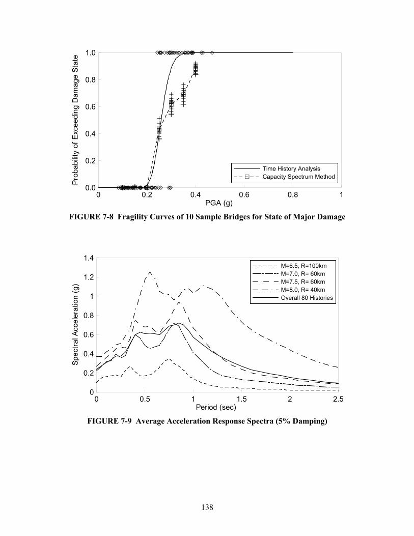
138
0 0.2 0.4 0.6 0.8 1PGA (g)
0.0
0.2
0.4
0.6
0.8
1.0
Prob
abilit
y of
Exc
eedi
ng D
amag
e St
ate
Time History AnalysisCapacity Spectrum Method
FIGURE 7-8 Fragility Curves of 10 Sample Bridges for State of Major Damage
0 0.5 1 1.5 2 2.5Period (sec)
0
0.2
0.4
0.6
0.8
1
1.2
1.4
Spec
tral A
ccel
erat
ion
(g)
M=6.5, R=100kmM=7.0, R= 60kmM=7.5, R= 60kmM=8.0, R= 40kmOverall 80 Histories
FIGURE 7-9 Average Acceleration Response Spectra (5% Damping)
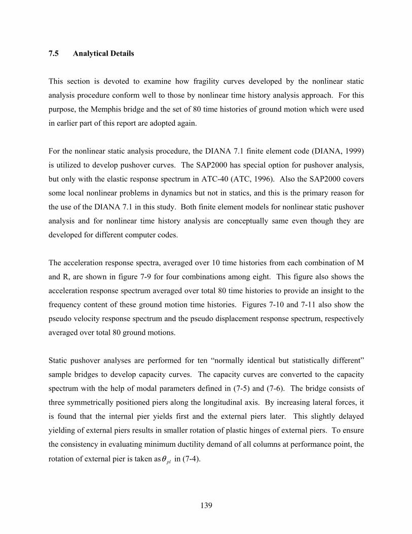
139
7.5 Analytical Details
This section is devoted to examine how fragility curves developed by the nonlinear static
analysis procedure conform well to those by nonlinear time history analysis approach. For this
purpose, the Memphis bridge and the set of 80 time histories of ground motion which were used
in earlier part of this report are adopted again.
For the nonlinear static analysis procedure, the DIANA 7.1 finite element code (DIANA, 1999)
is utilized to develop pushover curves. The SAP2000 has special option for pushover analysis,
but only with the elastic response spectrum in ATC-40 (ATC, 1996). Also the SAP2000 covers
some local nonlinear problems in dynamics but not in statics, and this is the primary reason for
the use of the DIANA 7.1 in this study. Both finite element models for nonlinear static pushover
analysis and for nonlinear time history analysis are conceptually same even though they are
developed for different computer codes.
The acceleration response spectra, averaged over 10 time histories from each combination of M
and R, are shown in figure 7-9 for four combinations among eight. This figure also shows the
acceleration response spectrum averaged over total 80 time histories to provide an insight to the
frequency content of these ground motion time histories. Figures 7-10 and 7-11 also show the
pseudo velocity response spectrum and the pseudo displacement response spectrum, respectively
averaged over total 80 ground motions.
Static pushover analyses are performed for ten “normally identical but statistically different”
sample bridges to develop capacity curves. The capacity curves are converted to the capacity
spectrum with the help of modal parameters defined in (7-5) and (7-6). The bridge consists of
three symmetrically positioned piers along the longitudinal axis. By increasing lateral forces, it
is found that the internal pier yields first and the external piers later. This slightly delayed
yielding of external piers results in smaller rotation of plastic hinges of external piers. To ensure
the consistency in evaluating minimum ductility demand of all columns at performance point, the
rotation of external pier is taken as plθ in (7-4).
140
The modal parameters in (7-5) and (7-6) gradually change while the plastic hinges undergo
beyond the yielding limit. Hence, modal parameters are calculated in several loading states and
linearly interpolated between the calculated points. These modal parameters are calculated on or
near the ductility demand of plastic hinge equal to 1, 2, 3, 4 and 10. Fundamental natural periods
of 10 bridges at these ductility demands are calculated using (7-2) and presented in figure 7-12.
As shown in this figure, the fundamental natural periods for 10 bridges fall into the range from
1.2 sec to 3.0 sec approximately. Finally, figure 7-1 shows capacity spectra for the ten sample
bridges.
Figures 7-2 and 7-3 show the m and σ±m ADRS for PGA=0.25g and 0.40g, respectively. The
spectral displacement, dS can be determined by plotting the capacity spectrum on the same
ADRS coordinates. Figures 7-4~7-6 show the representative procedure to evaluate the
performance displacements for the m and σ±m ADRS which are defined as dS and ddS σ± ,
respectively.
The mean ( dS ) and mean ± standard deviation ( ddS σ± ) of displacement of one sample bridge
for each PGA are shown in figure 7-13. This figure shows that dS , +dσ and −
dσ increase
gradually as PGA increases. It is also found that the magnitude of +dσ at any PGA is not same
as that of −dσ . In other words, the distribution of displacement according to PGA is not
symmetric. This study assumes that the performance displacement has the mean dS and
standard deviation dσ redefined by ( )( )−+dd σσ . The two-parameters, c and ζ of lognormal
distribution are obtained using (7-11) and (7-12) with dσ as defined here. The probability that
each bridge will be in a state of specified damage is calculated using (7-14) for each damage
state. The final fragility value is obtained from (7-15) by taking into consideration all the
bridges in each PGA group at the corresponding value of PGA.
Figure 7-7 shows the fragility curves associated with state of at least minor damage developed by
two methods. Eighty diamonds plotted on the two horizontal axes and the fragility curve by time
history method are replotted here from the earlier part of this report. The open squares in figure
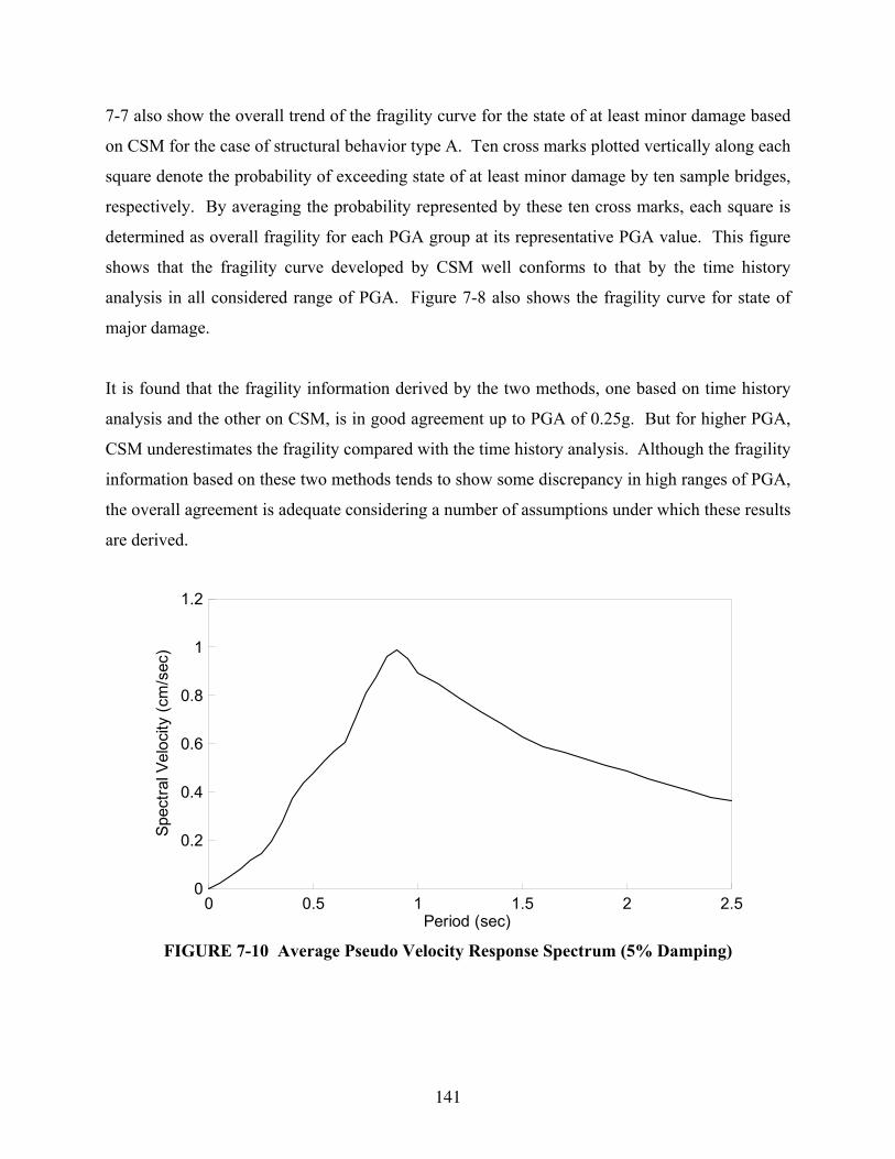
141
7-7 also show the overall trend of the fragility curve for the state of at least minor damage based
on CSM for the case of structural behavior type A. Ten cross marks plotted vertically along each
square denote the probability of exceeding state of at least minor damage by ten sample bridges,
respectively. By averaging the probability represented by these ten cross marks, each square is
determined as overall fragility for each PGA group at its representative PGA value. This figure
shows that the fragility curve developed by CSM well conforms to that by the time history
analysis in all considered range of PGA. Figure 7-8 also shows the fragility curve for state of
major damage.
It is found that the fragility information derived by the two methods, one based on time history
analysis and the other on CSM, is in good agreement up to PGA of 0.25g. But for higher PGA,
CSM underestimates the fragility compared with the time history analysis. Although the fragility
information based on these two methods tends to show some discrepancy in high ranges of PGA,
the overall agreement is adequate considering a number of assumptions under which these results
are derived.
0 0.5 1 1.5 2 2.5Period (sec)
0
0.2
0.4
0.6
0.8
1
1.2
Spec
tral V
eloc
ity (c
m/s
ec)
FIGURE 7-10 Average Pseudo Velocity Response Spectrum (5% Damping)
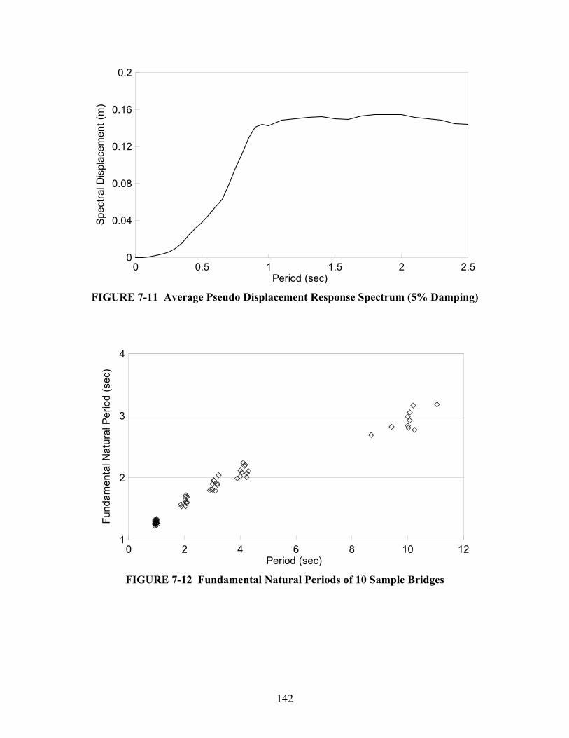
142
0 0.5 1 1.5 2 2.5Period (sec)
0
0.04
0.08
0.12
0.16
0.2
Spec
tral D
ispl
acem
ent (
m)
FIGURE 7-11 Average Pseudo Displacement Response Spectrum (5% Damping)
0 2 4 6 8 10 12Period (sec)
1
2
3
4
Fund
amen
tal N
atur
al P
erio
d (s
ec)
FIGURE 7-12 Fundamental Natural Periods of 10 Sample Bridges
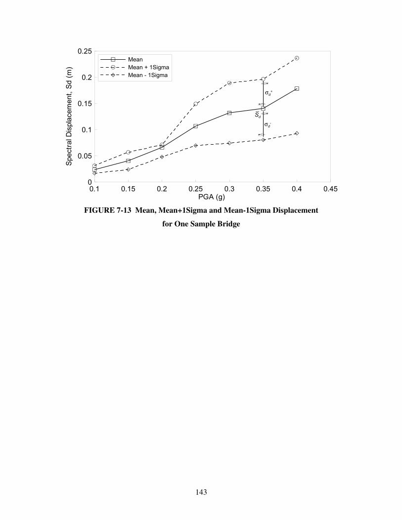
143
0.1 0.15 0.2 0.25 0.3 0.35 0.4 0.45PGA (g)
0
0.05
0.1
0.15
0.2
0.25
Spec
tral D
ispl
acem
ent,
Sd (m
)MeanMean + 1SigmaMean - 1Sigma
σd+
σd-Sd_
FIGURE 7-13 Mean, Mean+1Sigma and Mean-1Sigma Displacement
for One Sample Bridge

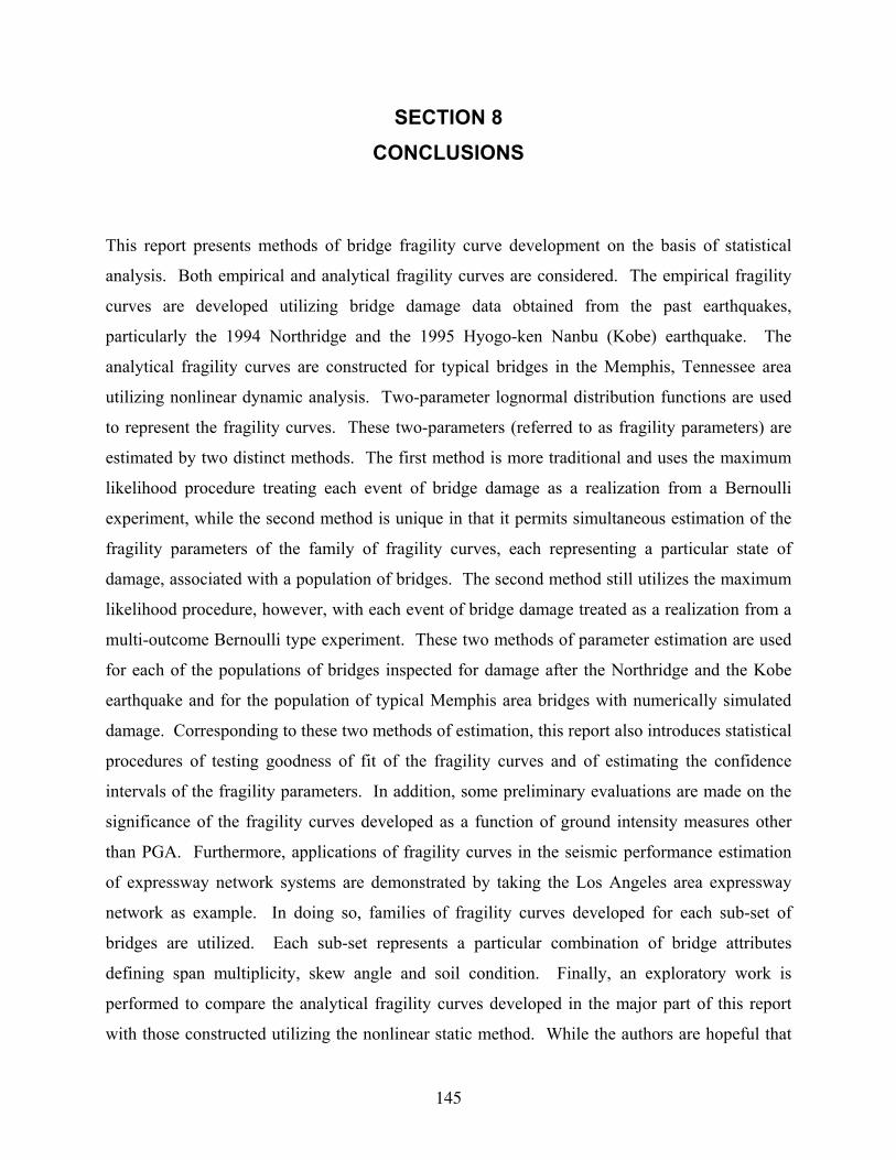
145
SECTION 8 CONCLUSIONS
This report presents methods of bridge fragility curve development on the basis of statistical
analysis. Both empirical and analytical fragility curves are considered. The empirical fragility
curves are developed utilizing bridge damage data obtained from the past earthquakes,
particularly the 1994 Northridge and the 1995 Hyogo-ken Nanbu (Kobe) earthquake. The
analytical fragility curves are constructed for typical bridges in the Memphis, Tennessee area
utilizing nonlinear dynamic analysis. Two-parameter lognormal distribution functions are used
to represent the fragility curves. These two-parameters (referred to as fragility parameters) are
estimated by two distinct methods. The first method is more traditional and uses the maximum
likelihood procedure treating each event of bridge damage as a realization from a Bernoulli
experiment, while the second method is unique in that it permits simultaneous estimation of the
fragility parameters of the family of fragility curves, each representing a particular state of
damage, associated with a population of bridges. The second method still utilizes the maximum
likelihood procedure, however, with each event of bridge damage treated as a realization from a
multi-outcome Bernoulli type experiment. These two methods of parameter estimation are used
for each of the populations of bridges inspected for damage after the Northridge and the Kobe
earthquake and for the population of typical Memphis area bridges with numerically simulated
damage. Corresponding to these two methods of estimation, this report also introduces statistical
procedures of testing goodness of fit of the fragility curves and of estimating the confidence
intervals of the fragility parameters. In addition, some preliminary evaluations are made on the
significance of the fragility curves developed as a function of ground intensity measures other
than PGA. Furthermore, applications of fragility curves in the seismic performance estimation
of expressway network systems are demonstrated by taking the Los Angeles area expressway
network as example. In doing so, families of fragility curves developed for each sub-set of
bridges are utilized. Each sub-set represents a particular combination of bridge attributes
defining span multiplicity, skew angle and soil condition. Finally, an exploratory work is
performed to compare the analytical fragility curves developed in the major part of this report
with those constructed utilizing the nonlinear static method. While the authors are hopeful that

146
the conceptual and theoretical treatment dealt in this study can provide theoretical basis and
analytical tools of practical usefulness for the development of fragility curves, there are many
analytical and implementational aspects that require further study including:
1. Physical definition of damage that can be used for post-earthquake damage inspection and
analysis.
2. Use of other measures of ground motion intensity than PGA for fragility curve development.
3. Bridge categorization based on physical attributes.
4. Further study on the use of nonlinear static analysis procedures for fragility curve
development.
5. Transportation systems analysis accounting for uncertainty in the fragility parameters.

147
SECTION 9 REFERENCES
1. ATC, (1996), “Seismic Evaluation and Retrofit of Concrete Buildings”, Report ATC-40, Applied Technology Council, Redwood City, CA.
2. ATC, (1985), “Earthquake Damage Evaluation Data for California”, Report ATC-13,
Applied Technology Council, Redwood City, CA. 3. Barron-Covera, Raul (1999), “Spectral Evaluation of Seismic Fragility of Structures”, Ph.D.
dissertation, Faculty of the Graduate School of the State University of New York at Buffalo. 4. Basoz, N. and Kiremidjian, A.S., (1998), “Evaluation of Bridge Damage Data from the
Loma Prieta and Northridge, California Earthquake”, Technical Report MCEER-98-0004. 5. Boore, D. M., (1983), “tochastic Simulation of High-frequency Ground Motions Based on
Seismological Models of the Radiation Spectra”, Bulletin of the Seismological Society of America, 73, 1865-1894.
6. Buckle, I. G., (1994), “The Northridge, California Earthquake of January 17, 1994:
Performance of Highway Bridges”, Technical Report NCEER-94-0008. 7. California Department of Transportation (Caltrans), (1994a), “The Northridge Earthquake”,
Caltrans PEQIT Report, Division of Structures, Sacramento, CA. 8. California Department of Transportation (Caltrans), (1994b), “Supplementary Bridge
Damage Reports”, Division of Structures, Sacramento, CA. 9. City of Los Angeles (COLA), (1995), “Earthquake Hazard Reduction in Existing
Reinforced Concrete Buildings and Concrete Frame Buildings with Masonry Infills”, Los Angeles, CA.
10. DIANA Finite Element Analysis User’s Manual; Release 7.1, (1999), TNO Building and
Construction Research, Delft, Netherlands. 11. Dutta, A. and Mander, J. B., (1998), “Seismic Fragility Analysis of Highway Bridges”,
INCEDE-MCEER Center-to-Center Workshop on Earthquake Engineering Frontiers in Transportation Systems, June 1998, Tokyo, Japan.
12. Federal Emergency Management Agency (FEMA), (1997a), “NEHRP Guidelines for the
Seismic Rehabilitation of Buildings”, FEMA-273, Washington, D.C.

148
13. Federal Emergency Management Agency (FEMA), (1997b), “NEHRP Commentary on the Guidelines for the Seismic Rehabilitation of Buildings”, FEMA-274, Washington, D.C.
14. Housner, G. W., (1952), “Spectrum Intensities of Strong Motion Earthquake”, Proceedings
of 1952 Symposium on Earthquake and Blast Effects on Structures, Earthquake Engineering Research Institute.
15. Hwang, H. M., and Huo, J. R., (1996), “Simulation of Earthquake Acceleration Time
Histories”, Center for Earthquake Research and Information, The University of Memphis, Technical Report.
16. Hwang, H. M., Lin, H. and Huo, J. R., (1997), “Seismic Performance Evaluation of Fire
Stations in Shelby County, Tennessee”, Earthquake Spectra, 13(4), 759-772. 17. Hwang, H. M. and Huo, J. R., (1998), “Modeling Uncertainty on Seismic Fragility of
Structures.” Structural Safety and Reliability, Shiraishi, Shinozuka, & Wen (eds.), A. A. Balkema, Rotterdam, 1721-1724.
18. Hwang H. M., Jernigan, J. B. and Lin, Y. W., (1999), “Expected Seismic Damage to
Memphis Highway Systems”, Proceedings of 5th U. S. Conference on Lifeline Earthquake Engineering, Seatle, WA, August 12-14, 1999, American Society of Civil Engineering, Reston, VA, 1-10.
19. Idriss, I. M., and Sun, J. I., (1992), "SHAKE91, A Computer Program for Conducting
Equivalent Linear Seismic Response Analyses of Horizontally Layered Soil Deposits, User's manual." Center for Geotechnical Modeling, Department of Civil and Environmental Engineering, University of California, Davis, CA.
20. Jernigan, J. B., and Hwang, H. M., (1997), "Inventory and Fragility Analysis of Memphis
Bridges", Center for Earthquake Research and Information, The University of Memphis, Technical Report.
21. Mizutani, M., (1999), Private Communication. 22. Nakamura, T., and Mizatani, M., (1996), “A Statistical Method for Fragility Curve
Development”, Proceedings of the 51st JSCE Annual Meeting, Vol. 1-A, 938-939. 23. Nakamura, T., Naganuma, T., Shizuma, T. and Shinozuka, M., (1998), “A Study on Failure
Probability of Highway Bridges by Earthquake Based on Statistical Method.” to appear in Proceedings of the 10th Japanese Earthquake Engineering Symposium.
24. Shinozuka, M. and Deodatis, G., (1991), “Simulation of Stochastic Processes by Spectral
Representation”, Applied Mechanics Reviews, Vol. 44, No. 4, 191-204. 25. Shinozuka, M., Feng, M. Q., Lee, J. H. and Nagaruma, T., (1999), “ Statistical Analysis of
Fragility Curves”, Proceedings of the Asian-Pacific Symposium on Structural Reliability
149
and its application (APSSRA 99), Keynote Paper, Taipei, Taiwan, Republic of China, February 1-3, Accepted for Publication in Journal of Engineering Mechanics, ASCE.
26. Singhal, A. and Kiremidjian, A. S., (1997), “Bayesian Updating of Fragilities with
Application to RC Frames”, Accepted for publication in Journal of Structural Engineering, ASCE.
27. U.S. Nuclear Regulatory Commission (NRC), (1983), “PRA Procedures Guide”,
NUREG/CR-2300, Vol. 2, 11-46. 28. Wald, D. J., Quitoriano, V., Heaton, T. H., Kanamori, H., Scrivner, C. W. and Worden C. B.,
(1999), “TriNet ‘ShakeMaps’: Rapid Generation of Peak Ground Motion and Itensity Maps for Earthquakes in Southern California”, Earthquake Spectra, Vol.15, No.3, 537-556.


University at Buffalo The State University of New York
University at Buffalo, State University of New York
Red Jacket Quadrangle ■ Buffalo, New York 14261
Phone: (716) 645-3391 ■ Fax: (716) 645-3399
E-mail: [email protected] ■ WWW Site http://mceer.buffalo.edu
ISSN 1520-295X


![Development of fragility curves for existing residential ...scientiairanica.sharif.edu/article_21498_1b4140b0a40ae864af4f4741123bf662.pdfthree-dimensionally in OpenSees [18]. E ort](https://static.fdocuments.net/doc/165x107/6049a4e6007677277e1f9238/development-of-fragility-curves-for-existing-residential-three-dimensionally.jpg)