Statistical AnalysisHandbook

A Comprehensive Handbook of StatisticalConcepts, Techniques and Software Tools

2018 Edition

Dr Michael J de Smith

Statistical AnalysisHandbook

A Comprehensive Handbook of StatisticalConcepts, Techniques and Software Tools

Dr Michael J de Smith

No part of this publication may be reproduced, stored in a retrieval system or transmitted in any form

or by any means, electronic, mechanical, photocopying, recording, scanning or otherwise, except

under the terms of the UK Copyright Designs and Patents Act 1998 or with the written permission of

the authors. The moral right of the authors has been asserted. Copies of this edition are available in

electronic book and web-accessible formats only.

Disclaimer: This publication is designed to offer accurate and authoritative information in regard to

the subject matter. It is provided on the understanding that it is not supplied as a form of professional

or advisory service. References to software products, datasets or publications are purely made for

information purposes and the inclusion or exclusion of any such item does not imply recommendation

or otherwise of the product or material in question.

For more details please refer to the Guide’s website: www.statsref.com

ISBN-13

978-1-912556-06-9 Hardback

978-1-912556-07-6 Paperback

978-1-912556-08-3 eBook

Published by: The Winchelsea Press, Drumlin Security Ltd, Edinburgh

Copyright © 2015-2018 All Rights reserved. 2018 Edition. Issue version: 2018-1

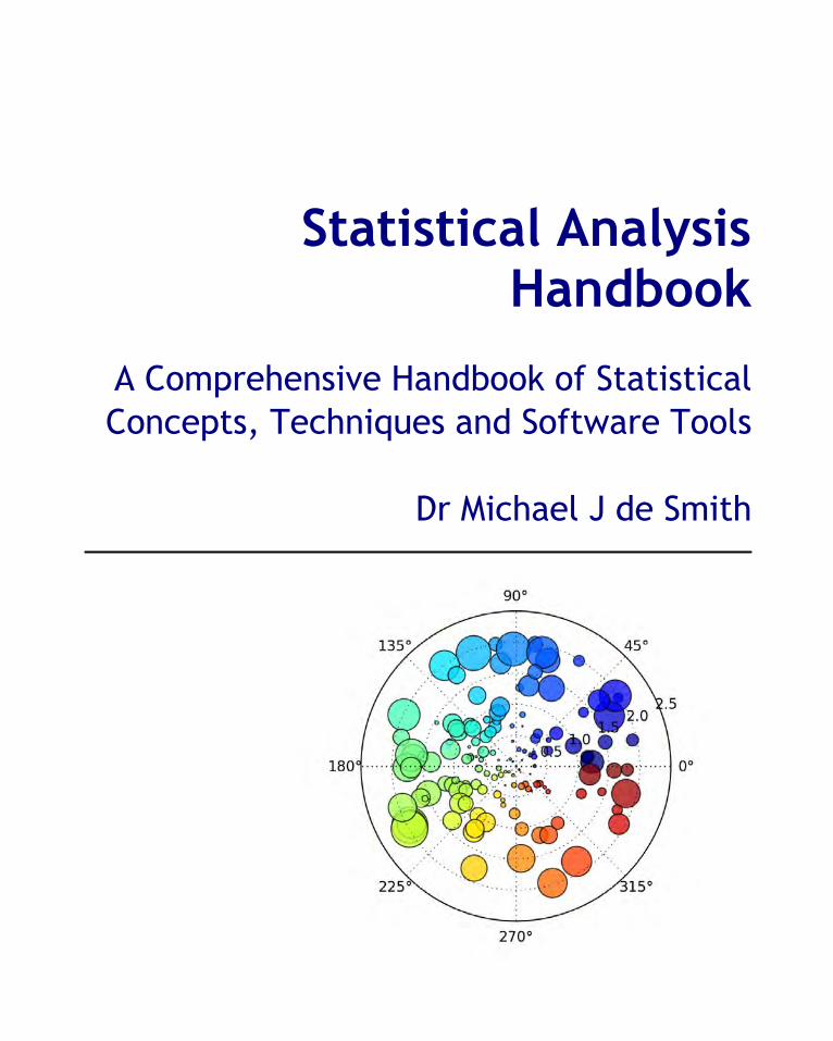
Front inside cover image: Polar bubble plot (MatPlotLib, Python)

Rear inside cover image: Florence Nightingale's polar diagram of causes of mortality, by month

(source: Wikipedia)

Cover image: Mandlebrot set fractal

5

www.statsref.com (c) 2018

Table of Contents

1 13Introduction

1.1 How to use this Handbook 17

1.2 Intended audience and scope 18

1.3 Suggested reading 19

1.4 Notation and symbology 23

1.5 Historical context 25

1.6 An applications-led discipline 31

2 37Statistical data

2.1 The Statistical Method 53

2.2 Misuse, Misinterpretation and Bias 60

2.3 Sampling and sample size 71

2.4 Data preparation and cleaning 80

2.5 Missing data and data errors 82

2.6 Statistical error 87

2.7 Statistics in Medical Research 88

90Causation 2.7.1

93Conduct and reporting of medical research 2.7.2

3 105Statistical concepts

3.1 Probability theory 108

109Odds 3.1.1

110Risks 3.1.2

112Frequentist probability theory 3.1.3

116Bayesian probability theory 3.1.4

120Probability distributions 3.1.5

3.2 Statistical modeling 122

3.3 Computational statistics 125

3.4 Inference 126

6

www.statsref.com (c) 2018

3.5 Bias 127

3.6 Confounding 129

3.7 Hypothesis testing 130

3.8 Types of error 132

3.9 Statistical significance 134

3.10 Confidence intervals 137

3.11 Power and robustness 141

3.12 Degrees of freedom 142

3.13 Non-parametric analysis 143

4 145Descriptive statistics

4.1 Counts and specific values 148

4.2 Measures of central tendency 150

4.3 Measures of spread 157

4.4 Measures of distribution shape 166

4.5 Statistical indices 170

4.6 Moments 172

5 175Key functions and expressions

5.1 Key functions 178

5.2 Measures of Complexity and Model selection 185

5.3 Matrices 190

6 199Data transformation and standardization

6.1 Box-Cox and Power transforms 202

6.2 Freeman-Tukey (square root and arcsine) transforms 204

6.3 Log and Exponential transforms 207

6.4 Logit transform 210

6.5 Normal transform (z-transform) 212

7 213Data exploration

7.1 Graphics and vizualisation 216

7

www.statsref.com (c) 2018

7.2 Exploratory Data Analysis 233

8 241Randomness and Randomization

8.1 Random numbers 245

8.2 Random permutations 254

8.3 Resampling 256

8.4 Runs test 260

8.5 Random walks 261

8.6 Markov processes 271

8.7 Monte Carlo methods 277

277Monte Carlo Integration 8.7.1

280Monte Carlo Markov Chains (MCMC) 8.7.2

9 285Correlation and autocorrelation

9.1 Pearson (Product moment) correlation 288

9.2 Rank correlation 298

9.3 Canonical correlation 302

9.4 Autocorrelation 304

305Temporal autocorrelation 9.4.1

310Spatial autocorrelation 9.4.2

10 333Probability distributions

10.1 Discrete Distributions 339

339Binomial distribution 10.1.1

343Hypergeometric distribution 10.1.2

345Multinomial distribution 10.1.3

347Negative Binomial or Pascal and Geometric distribution 10.1.4

349Poisson distribution 10.1.5

354Skellam distribution 10.1.6

355Zipf or Zeta distribution 10.1.7

10.2 Continuous univariate distributions 356

356Beta distribution 10.2.1

358Chi-Square distribution 10.2.2

361Cauchy distribution 10.2.3

8

www.statsref.com (c) 2018

362Erlang distribution 10.2.4

364Exponential distribution 10.2.5

367F distribution 10.2.6

369Gamma distribution 10.2.7

371Gumbel and extreme value distributions 10.2.8

374Normal distribution 10.2.9

379Pareto distribution 10.2.10

381Student's t-distribution (Fisher's distribution) 10.2.11

384Uniform distribution 10.2.12

386von Mises distribution 10.2.13

390Weibull distribution 10.2.14

10.3 Multivariate distributions 392

10.4 Kernel Density Estimation 396

11 405Estimation and estimators

11.1 Maximum Likelihood Estimation (MLE) 409

11.2 Bayesian estimation 414

12 417Classical tests

12.1 Goodness of fit tests 420

421Anderson-Darling 12.1.1

423Chi-square test 12.1.2

426Kolmogorov-Smirnov 12.1.3

428Ryan-Joiner 12.1.4

429Shapiro-Wilk 12.1.5

431Jarque-Bera 12.1.6

431Lilliefors 12.1.7

12.2 Z-tests 433

433Test of a single mean, standard deviation known 12.2.1

435Test of the difference between two means, standard deviations known 12.2.2

436Tests for proportions, p 12.2.3

12.3 T-tests 438

438Test of a single mean, standard deviation not known 12.3.1

439Test of the difference between two means, standard deviation not known 12.3.2

440Test of regression coefficients 12.3.3

9

www.statsref.com (c) 2018

12.4 Variance tests 443

443Chi-square test of a single variance 12.4.1

444F-tests of two variances 12.4.2

445Tests of homogeneity 12.4.3

12.5 Wilcoxon rank-sum/Mann-Whitney U test 449

12.6 Sign test 453

13 455Contingency tables

13.1 Chi-square contingency table test 459

13.2 G contingency table test 461

13.3 Fisher's exact test 462

13.4 Measures of association 465

13.5 McNemar's test 466

14 467Design of experiments

14.1 Completely randomized designs 475

14.2 Randomized block designs 476

477Latin squares 14.2.1

479Graeco-Latin squares 14.2.2

14.3 Factorial designs 481

481Full Factorial designs 14.3.1

483Fractional Factorial designs 14.3.2

485Plackett-Burman designs 14.3.3

14.4 Regression designs and response surfaces 487

14.5 Mixture designs 489

15 491Analysis of variance and covariance

15.1 ANOVA 496

500Single factor or one-way ANOVA 15.1.1

504Two factor or two-way and higher-way ANOVA 15.1.2

15.2 MANOVA 507

15.3 ANCOVA 509

15.4 Non-Parametric ANOVA 510

10

www.statsref.com (c) 2018

510Kruskal-Wallis ANOVA 15.4.1

512Friedman ANOVA test 15.4.2

513Mood's Median 15.4.3

16 515Regression and smoothing

16.1 Least squares 522

16.2 Ridge regression 528

16.3 Simple and multiple linear regression 529

16.4 Polynomial regression 543

16.5 Generalized Linear Models (GLIM) 545

16.6 Logistic regression for proportion data 547

16.7 Poisson regression for count data 550

16.8 Non-linear regression 554

16.9 Smoothing and Generalized Additive Models (GAM) 558

16.10 Geographically weighted regression (GWR) 560

16.11 Spatial series and spatial autoregression 565

571SAR models 16.11.1

575CAR models 16.11.2

579Spatial filtering models 16.11.3

17581

Time series analysis and temporalautoregression

17.1 Moving averages 588

17.2 Trend Analysis 593

17.3 ARMA and ARIMA (Box-Jenkins) models 599

17.4 Spectral analysis 608

18 611Resources

18.1 Distribution tables 614

18.2 Bibliography 629

18.3 Statistical Software 638

18.4 Test Datasets and data archives 640

18.5 Websites 653

11

www.statsref.com (c) 2018

18.6 Tests Index 654

654Tests and confidence intervals for mean values 18.6.1

654Tests for proportions 18.6.2

655Tests and confidence intervals for the spread of datasets 18.6.3

655Tests of randomness 18.6.4

655Tests of fit to a given distribution 18.6.5

656Tests for cross-tabulated count data 18.6.6

18.7 R Code samples 657

657Scatter Plot: Inequality 18.7.1

658Latin Square ANOVA 18.7.2

659Log Odds Ratio Plot 18.7.3

660Normal distribution plot 18.7.4

660Bootstrapping 18.7.5

Chapter

1

Introduction 15

www.statsref.com (c) 2018

1 Introduction

The definition of what is meant by statistics and statistical analysis has changed considerably over the last few

decades. Here are two contrasting definitions of what statistics is, from eminent professors in the field, some 60+

years apart:

"Statistics is the branch of scientific method which deals with the data obtained by counting or measuring the

properties of populations of natural phenomena. In this definition 'natural phenomena' includes all the

happenings of the external world, whether human or not." Professor Maurice Kendall, 1943, p2 [MK1]

"Statistics is: the fun of finding patterns in data; the pleasure of making discoveries; the import of deep

philosophical questions; the power to shed light on important decisions, and the ability to guide decisions.....

in business, science, government, medicine, industry..." Professor David Hand [DH1]

As these two definitions indicate, the discipline of statistics has moved from being grounded firmly in the world of

measurement and scientific analysis into the world of exploration, comprehension and decision-making. At the

same time its usage has grown enormously, expanding from a relatively small set of specific application areas

(such as design of experiments and computation of life insurance premiums) to almost every walk of life. A

particular feature of this change is the massive expansion in information (and misinformation) available to all

sectors and age-groups in society. Understanding this information, and making well-informed decisions on the

basis of such understanding, is the primary function of modern statistical methods.

Our objective in producing this Handbook is to be comprehensive in terms of concepts and techniques (but not

necessarily exhaustive), representative and independent in terms of software tools, and above all practical in

terms of application and implementation. However, we believe that it is no longer appropriate to think of a

standard, discipline-specific textbook as capable of satisfying every kind of new user need. Accordingly, an

innovative feature of our approach here is the range of formats and channels through which we disseminate the

material — web, ebook and print. A major advantage of the electronic formats is that the text can be embedded

with internal and external hyperlinks (shown underlined). In this Handbook we utilize both forms of link, with

external links often referring to a small number of well-established sources, including MacTutor for bibliographic

information and a number of other web resources, such as Eric Weisstein's Mathworld and the statistics portal of

Wikipedia, that provide additional material on selected topics.

The treatment of topics in this Handbook is relatively informal, in that we do not provide mathematical proofs for

much of the material discussed. However, where it is felt particularly useful to clarify how an expression arises,

we do provide simple derivations. More generally we adopt the approach of using descriptive explanations and

worked examples in order to clarify the usage of different measures and procedures. Frequently convenient

software tools are used for this purpose, notably SPSS/PASW, The R Project, MATLab and a number of more

specialized software tools where appropriate.

Just as all datasets and software packages contain errors, known and unknown, so too do all books and websites,

and we expect that there will be errors despite our best efforts to remove these! Some may be genuine errors or

misprints, whilst others may reflect our use of specific versions of software packages and their documentation.

Inevitably with respect to the latter, new versions of the packages that we have used to illustrate this Handbook

will have appeared even before publication, so specific examples, illustrations and comments on scope or

restrictions may have been superseded. In all cases the user should review the documentation provided with the

16

www.statsref.com (c) 2018

software version they plan to use, check release notes for changes and known bugs, and look at any relevant

online services (e.g. user/developer forums and blogs on the web) for additional materials and insights.

The interactive web and PDF versions of this Handbook provide color images and active hyperlinks, and may be

accessed via the associated Internet site: www.statsref.com. The contents and sample sections of the PDF version

may also be accessed from this site. In both cases the information is regularly updated. The Internet is now well

established as society’s principal mode of information exchange, and most aspiring users of statistical methods are

accustomed to searching for material that can easily be customized to specific needs. Our objective for such users

is to provide an independent, reliable and authoritative first port of call for conceptual, technical, software and

applications material that addresses the panoply of new user requirements.

Readers wishing to obtain a more in-depth understanding of the background to many of the topics covered in this

Handbook should review the Suggested Reading topic.

References

[DH1] D Hand (2009) President of the Royal Statistical Society (RSS), RSS Conference Presentation, November 2009

[MK1] Kendall M G, Stuart A (1943) The Advanced Theory of Statistics: Volume 1, Distribution Theory. Charles Griffin &

Company, London. First published in 1943, revised in 1958 with Stuart

Introduction 17

www.statsref.com (c) 2018

1.1 How to use this Handbook

This Handbook is designed to provide a wide-ranging and comprehensive, though not exhaustive, coverage of

statistical concepts and methods. Unlike a Wiki the Handbook has a more linear flow structure, and in principle

can be read from start to finish. In practice many of the topics, particularly some of those described in later parts

of the document, will be of interest only to specific users at particular times, but are provided for completeness.

Users are recommended to read the initial four topics — Introduction, Statistical Concepts, Statistical Data and

Descriptive Statistics, and then select subsequent sections as required.

Navigating around the PDF or web versions of this Handbook is straightforward, but to assist this process a number

of special facilities have been built into the design to make the process even easier. These facilities include:

· Tests Index — this is a form of 'how to' index, i.e. it does not assume that the reader knows the name of the test

they may need to use, but can navigate to the correct item by the index description

· Reference links and bibliography — within the text all books and articles referenced are linked to the full

reference at the end of the topic section (in the References subsection) in the format [XXXn] and in the

complete bibliography at the end of the Handbook

· Hyperlinks — within the document there are two types of hyperlink: (i) internal hyperlinks — when clicking on

these links you will be directed to the linked topic within this Handbook; (ii) external hyperlinks — these

provide access to external resources for which you need an active internet connection. When the external links

are clicked the appropriate topic is opened on an external website such as Wikipedia

· Search facilities — the web and PDF versions of this Handbook facilitate free text search, so as long as you know

roughly what you are looking for, you should be able to find it using this facility

Intended audience and scope18

www.statsref.com (c) 2018

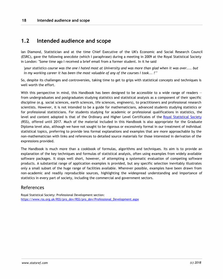
1.2 Intended audience and scope

Ian Diamond, Statistician and at the time Chief Executive of the UK's Economic and Social Research Council

(ESRC), gave the following anecdote (which I paraphrase) during a meeting in 2009 at the Royal Statistical Society

in London: "Some time ago I received a brief email from a former student. In it he said

'your statistics course was the one I hated most at University and was more than glad when it was over.... but

in my working career it has been the most valuable of any of the courses I took... !'"

So, despite its challenges and controversies, taking time to get to grips with statistical concepts and techniques is

well worth the effort.

With this perspective in mind, this Handbook has been designed to be accessible to a wide range of readers —

from undergraduates and postgraduates studying statistics and statistical analysis as a component of their specific

discipline (e.g. social sciences, earth sciences, life sciences, engineers), to practitioners and professional research

scientists. However, it is not intended to be a guide for mathematicians, advanced students studying statistics or

for professional statisticians. For students studying for academic or professional qualifications in statistics, the

level and content adopted is that of the Ordinary and Higher Level Certificates of the Royal Statistical Society

(RSS), offered until 2017. Much of the material included in this Handbook is also appropriate for the Graduate

Diploma level also, although we have not sought to be rigorous or excessively formal in our treatment of individual

statistical topics, preferring to provide less formal explanations and examples that are more approachable by the

non-mathematician with links and references to detailed source materials for those interested in derivation of the

expressions provided.

The Handbook is much more than a cookbook of formulas, algorithms and techniques. Its aim is to provide an

explanation of the key techniques and formulas of statistical analysis, often using examples from widely available

software packages. It stops well short, however, of attempting a systematic evaluation of competing software

products. A substantial range of application examples is provided, but any specific selection inevitably illustrates

only a small subset of the huge range of facilities available. Wherever possible, examples have been drawn from

non-academic and readily reproducible sources, highlighting the widespread understanding and importance of

statistics in every part of society, including the commercial and government sectors.

References

Royal Statistical Society: Professional Development section:

https://www.rss.org.uk/RSS/pro_dev/RSS/pro_dev/Professional_Development.aspx

Introduction 19

www.statsref.com (c) 2018

1.3 Suggested reading

There are a vast number of books on statistics — Amazon alone lists 10,000+ "professional and technical" works

with statistics in their title. There is no single book or website on statistics that meets the need of all levels and

requirements of readers, so the answer for many people starting out will be to acquire the main 'set books'

recommended by their course tutors and then to supplement these with works that are specific to their

application area. Every topic and subtopic in this Handbook almost certainly has at least one entire book devoted

to it, so of necessity the material we cover can only provide the essential details and a starting point for deeper

understanding of each topic. As far as possible we provide links to articles, web sites, books and software

resources to enable the reader to pursue such questions as and when they wish.

Most statistics texts do not make for easy or enjoyable reading! In general they address difficult technical and

philosophical issues, and many are demanding in terms of their mathematics. Others are much more approachable

— these books include 'classic' undergraduate text books such as Feller (1950, [FEL1]), Mood and Graybill (1950,

[MOO1]), Hoel (1947, [HOE1]), Adler and Roessler (1960, [ADL1]), Brunk (1960, [BRU1]), Snedecor and Cochrane

(1937, [SNE1]) and Yule and Kendall (1950, [YUL1]) — the dates cited in each case are when the books were

originally published; in most cases these works then ran into many subsequent editions and though most are now

out-of-print some are still available. A more recent work, available from the American Mathematical Society and

also as a free PDF, is Grinstead and Snell's (1997) An Introduction to Probability [GRI1]. Still in print, and of

continuing relevance today, is Huff (1954, [HUF1]) "How to Lie with Statistics" which must be the top selling

statistics book of all time. A more recent book, with a similar focus, is Blastland and Dilnot's "The Tiger that

Isn't" [BLA1], which is full of examples of modern-day use and misuse of statistics. Another delightful, lighter

weight book that remains very popular, is Gonik and Smith's "Cartoon Guide to Statistics" (one of a series of such

cartoon guides by Gonik and co-authors, [GON1]). A very useful quick guide is the foldable free PDF format leaflet

"Probability & Statistics, Facts and Formulae" published by the UK Maths, Stats and OR Network [UKM1]. The free

Statistics Guide for Lawyers (PDF) available on the RSS website is a highly recommended resource (RSS and ICCA)

for both lawyers and non-lawyers alike.

Essential reading for anyone planning to use the free and remarkable "R Project" statistical resource is Crawley's

"The R Book" (2007, 2015 [CRA1]) and associated data files; and for students undertaking an initial course in

statistics using SPSS, Andy Field's "Discovering Statistics Using SPSS" provides a gentle introduction with many

worked examples and illustrations [FIE1]. Both Field and Crawley's books are large — around 900 pages in each

case. Data obtained in the social and behavioral sciences do not generally conform to the strict requirements of

traditional (parametric) inferential statistics and often require the use of methods that relax these requirements.

These so-called nonparametric methods are described in detail in Siegel and Castellan's widely used text

"Nonparametric Statistics for the Behavioral Sciences" (1998, [SIE1]) and Conover's "Practical Nonparametric

Statistics" (1999, [CON1]).

A key aspect of any statistical investigation is the use of graphics and visualization tools, and although technology

is changing this field Tufte's "The Visual Display of Quantitative Information" [TUF1] should be considered as

essential reading, despite its origins in the 1980s and the dramatic changes to visualization possibilities since its

publication.

With a more practical, applications focus, readers might wish to look at classics such as Box et al. (1978, 2005,

[BOX1]) "Statistics for Experimenters" (highly recommended, particularly for those involved in industrial

processes), Sokal and Rohlf (1995, [SOK1]) on Biometrics, and the now rather dated book on Industrial Production

Suggested reading20

www.statsref.com (c) 2018

edited by Davies (1961, [DAV1]) and partly written by the extraordinary George Box whilst a postgraduate student

at University College London. Box went on to a highly distinguished career in statistics, particular in industrial

applications, and is the originator of many statistical techniques and author of several groundbreaking books. He

not only met and worked with R A Fisher but later married one of Fisher's daughters! Crow et al. (1960, reprinted

in 2003, [CRO1]) published a concise but exceptionally clear "Statistics Manual" designed for use by the US Navy,

with most of its examples relating to ordnance — it provides a very useful and compact guide for non-statisticians

working in a broad range of scientific and engineering fields.

Taking a further step towards more demanding texts, appropriate for mathematics and statistics graduates and

post-graduates, we would recommend Kendall's Library of Statistics [KEN1], a multi-volume authoritative series

each volume of which goes into great detail on the area of statistics it focuses upon. For information on statistical

distributions we have drawn on a variety of sources, notably the excellent series of books by Johnson and Kotz

[JON1], [JON2] originally published in 1969/70. The latter authors are also responsible for the comprehensive but

extremely expensive nine volume "Encyclopedia of Statistical Sciences" (1998, 2006, [KOT1]). A much more

compact book of this type, with very brief but clear descriptions of around 500 topics, is the "Concise

Encyclopedia of Statistics" by Dodge (2002, [DOD1]).

With the rise of the Internet, web resources on statistical matters abound. However, it was the lack of a single,

coherent and comprehensive Internet resource that was a major stimulus to the current project. The present

author's book/ebook/website www.spatialanalysisonline.com has been extremely successful in providing

information on Geospatial Analysis to a global audience, but its focus on 2- and 3-dimensional spatial problems

limits its coverage of statistical topics. However, a significant percentage of Internet search requests that lead

users to this site involve queries about statistical concepts and techniques, suggesting a broader need for such

information in a suitable range of formats, which is what this Handbook attempts to provide.

A number of notable web-based resources providing information on statistical methods and formulas should be

mentioned. The first is Eric Weisstein's excellent Mathworld site, which has a large technical section on probability

and statistics. Secondly there is Wikipedia (Statistics section) — this is a fantastic resource, but is almost by

definition not always consistent or entirely independent. This is particularly noticeable for topics whose principal

or original authorship reflects the individual's area of specialism: social science, physics, biological sciences,

mathematics, economics etc, and in some instances their commercial background (e.g. for specific software

packages). Both Mathworld and Wikipedia provide a topic-by-topic structure, with little or no overall guide or flow

to direct users through the maze of topics, techniques and tools, although Wikipedia's core structure is very well

defined. This contrasts with the last two of our recommended websites: the NIST/SEMATECH online Engineering

Statistics e-Handbook, and the UCLA Statistics Online Computational Resource (SOCR). These latter resources are

much closer to our Handbook concept, providing information and guidance on a broad range of topics in a lucid,

structured and discursive manner. These sites have a further commonality with our project — their use of

particular software tools to illustrate many of the techniques and visualizations discussed. In the case of

NIST/SEMATECH e-Handbook a single software tool is used, Dataplot, which is a fairly basic, free, cross-platform

tool developed and maintained by the NIST. The UCLA Statistics Online Computational Resource project makes

extensive use of interactive Java applets to deliver web-enabled statistical tools. The present Handbook

references a wider range of software tools to illustrate its materials, including Dataplot, R, SPSS, Excel and

XLStat, MATLab, Minitab, SAS/STAT and many others. This enables us to provide a broader ranging commentary on

the toolsets available, and to compare the facilities and algorithms applied by the different implementations.

Throughout this Handbook we make extensive reference to functions and examples available in R, MATLab and

SPSS in particular.

Introduction 21

www.statsref.com (c) 2018

References

[ADL1] Adler H L, Roessler E B (1960) Introduction to Probability and Statistics. W H Freeman & Co, San Francisco

[BLA1] Blastland M, Dilnot A (2008) The Tiger That Isn't. Profile Books, London

[BOX1] Box G E P, Hunter J S, Hunter W G (1978) Statistics for Experimenters: An Introduction to Design, Data Analysis and

Model Building. J Wiley & Sons, New York. The second, extended edition was published in 2005

[BRU1] Brunk H D (1960) An Introduction to Mathematical Statistics. Blaisdell Publishing, Waltham, Mass.

[CHA1] Chatfield C (1975) The Analysis of Times Series: Theory and Practice. Chapman and Hall, London, UK (see also, extended

6th ed.)

[CON1] Conover W J (1999) Practical Nonparametric Statistics. 3rd ed., J Wiley & Sons, New York

[CRA1] Crawley M J (2007) The R Book. J Wiley & Son, Chichester, UK. 2nd ed. published in 2015

[CRO1] Crow E L, Davis F A, Maxfield M W (1960) Statistics Manual. Dover Publications. Reprinted in 2003 and still available

[DAV1] Davies O L ed. (1961) Statistical Methods in Research and Production. 3rd ed., Oliver & Boyd, London

[DOD1] Dodge Y (2002) The Concise Encyclopedia of Statistics. Springer, New York

[FEL1] Feller W (1950) An Introduction to Probability Theory and Its Applications. Vols 1 and 2. J Wiley & Sons

[FIE1] Field A (2009) Discovering Statistics Using SPSS. 3rd ed., Sage Publications

[GON1] Gonik L, Smith W (1993) Cartoon Guide to Statistics. Harper Collins, New York

[GRI1] Grinstead C M, Snell J L (1997) Introduction to Probability, 2nd ed. AMS, 1997

[HOE1] Hoel P G (1947) An Introduction to Mathematical Statistics. J Wiley & Sons, New York

[HUF1] Huff D (1954) How to Lie with Statistics. W.W. Norton & Co, New York

[JON1] Johnson N L, Kotz S (1969) Discrete distributions. J Wiley & Sons, New York. Note that a 3rd edition of this work, with

revisions and extensions, is published by J Wiley & Sons (2005) with the additional authorship of Adrienne Kemp of the

University of St Andrews.

[JON2] Johnson N L, Kotz S (1970) Continuous Univariate Distributions — 1 & 2. Houghton-Mifflin, Boston

[KEN1] Kendall M G, Stuart A (1943) The Advanced Theory of Statistics: Volume 1, Distribution Theory. Charles Griffin &

Company, London. First published in 1943, revised in 1958 with Stuart

[KOT1] Kotz S, Johnson L (eds.) (1988) Encyclopedia of Statistical Sciences. Vols 1-9, J Wiley & Sons, New York. A 2nd edition

with almost 10,000 pages was published with Kotz as the Editor-in-Chief, in 2006

[MAK1] Mackay R J, Oldford R W (2002) Scientific method, Statistical method and the Speed of Light, Working Paper 2002-02,

Dept of Statistics and Actuarial Science, University of Waterloo, Canada. An excellent paper that provides an insight into

Michelson’s 1879 experiment and explanation of the role and method of statistics in the larger context of science

[MOO1] Mood A M, Graybill F A (1950) Introduction to the Theory of Statistics. McGraw-Hill, New York

[SIE1] Siegel S, Castellan N J (1998) Nonparametric Statistics for the Behavioral Sciences. 2nd ed., McGraw Hill, New York

[SNE1] Snedecor G W, Cochran W G (1937) Statistical Methods. Iowa State University Press. Many editions

[SOK1] Sokal R R, Rohlf F J (1995) Biometry: The Principles and Practice of Statistics in Biological Research. 2nd ed., W H

Freeman & Co, New York

[TUF1] Tufte E R (2001) The Visual Display of Quantitative Information. 2nd edition. Graphics Press, Cheshire, Conn.

[UKM1] UK Maths, Stats & OR Network. Guides to Statistical Information: Probability and statistics Facts and Formulae.

http://icse.xyz/mathstore/index.html

Suggested reading22

www.statsref.com (c) 2018

[YUL1] Yule G U, Kendall M G (1950) An Introduction to the Theory of Statistics. Griffin, London, 14th edition (first edition was

published in 1911 under the sole authorship of Yule)

Web sites:

Mathworld: http://mathworld.wolfram.com/

NIST/SEMATECH e-Handbook of Statistical Methods: http://www.itl.nist.gov/div898/handbook/

UCLA Statistics Online Computational Resource (SOCR) : http://socr.ucla.edu/SOCR.html

Wikipedia: http://en.wikipedia.org/wiki/Statistics

Introduction 23

www.statsref.com (c) 2018

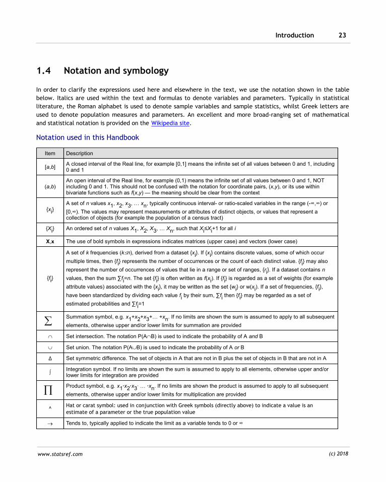
1.4 Notation and symbology

In order to clarify the expressions used here and elsewhere in the text, we use the notation shown in the table

below. Italics are used within the text and formulas to denote variables and parameters. Typically in statistical

literature, the Roman alphabet is used to denote sample variables and sample statistics, whilst Greek letters are

used to denote population measures and parameters. An excellent and more broad-ranging set of mathematical

and statistical notation is provided on the Wikipedia site.

Notation used in this Handbook

Item Description

[a,b]A closed interval of the Real line, for example [0,1] means the infinite set of all values between 0 and 1, including0 and 1

(a,b)An open interval of the Real line, for example (0,1) means the infinite set of all values between 0 and 1, NOTincluding 0 and 1. This should not be confused with the notation for coordinate pairs, (x,y), or its use withinbivariate functions such as f(x,y) — the meaning should be clear from the context

{xi}A set of n values x1, x2, x3, … xn, typically continuous interval- or ratio-scaled variables in the range (-∞,∞) or

[0,∞). The values may represent measurements or attributes of distinct objects, or values that represent acollection of objects (for example the population of a census tract)

{Xi} An ordered set of n values X1, X2, X3, … Xn, such that Xi≤Xi+1 for all i

X,x The use of bold symbols in expressions indicates matrices (upper case) and vectors (lower case)

{fi}

A set of k frequencies (k£n), derived from a dataset {xi}. If {xi} contains discrete values, some of which occur

multiple times, then {fi} represents the number of occurrences or the count of each distinct value. {fi} may also

represent the number of occurrences of values that lie in a range or set of ranges, {ri}. If a dataset contains n

values, then the sum ∑fi=n. The set {fi} is often written as f(xi). If {fi} is regarded as a set of weights (for example

attribute values) associated with the {xi}, it may be written as the set {wi} or w(xi). If a set of frequencies, {fi},

have been standardized by dividing each value fi by their sum, ∑fi then {fi} may be regarded as a set of

estimated probabilities and ∑fi=1

Summation symbol, e.g. x1+x2+x3+… +xn. If no limits are shown the sum is assumed to apply to all subsequent

elements, otherwise upper and/or lower limits for summation are provided

Ç Set intersection. The notation P(AÇB) is used to indicate the probability of A and B

È Set union. The notation P(AÈB) is used to indicate the probability of A or B

Δ Set symmetric difference. The set of objects in A that are not in B plus the set of objects in B that are not in A

ò Integration symbol. If no limits are shown the sum is assumed to apply to all elements, otherwise upper and/orlower limits for integration are provided

Product symbol, e.g. x1∙x2∙x3∙ … ∙xn. If no limits are shown the product is assumed to apply to all subsequent

elements, otherwise upper and/or lower limits for multiplication are provided

^Hat or carat symbol: used in conjunction with Greek symbols (directly above) to indicate a value is an

estimate of a parameter or the true population value

® Tends to, typically applied to indicate the limit as a variable tends to 0 or ∞

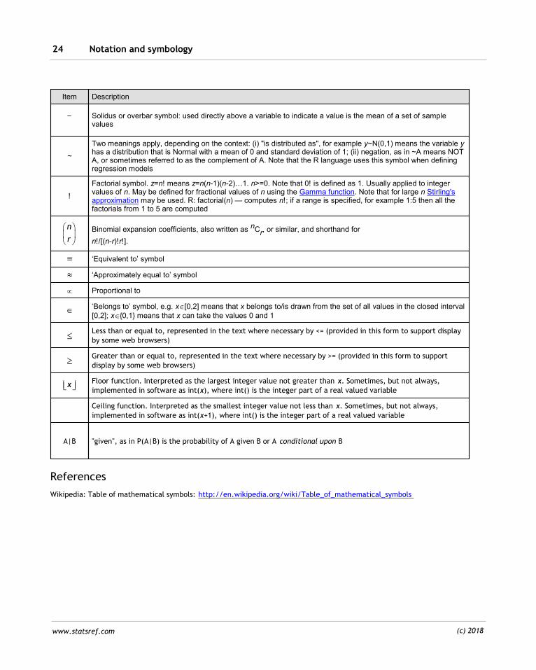
Notation and symbology24

www.statsref.com (c) 2018

Item Description

Solidus or overbar symbol: used directly above a variable to indicate a value is the mean of a set of samplevalues

~

Two meanings apply, depending on the context: (i) "is distributed as", for example y~N(0,1) means the variable yhas a distribution that is Normal with a mean of 0 and standard deviation of 1; (ii) negation, as in ~A means NOTA, or sometimes referred to as the complement of A. Note that the R language uses this symbol when definingregression models

!

Factorial symbol. z=n! means z=n(n-1)(n-2)…1. n>=0. Note that 0! is defined as 1. Usually applied to integervalues of n. May be defined for fractional values of n using the Gamma function. Note that for large n Stirling'sapproximation may be used. R: factorial(n) — computes n!; if a range is specified, for example 1:5 then all thefactorials from 1 to 5 are computed

n

r

Binomial expansion coefficients, also written as nCr, or similar, and shorthand for

n!/[(n-r)!r!].

‘Equivalent to’ symbol

‘Approximately equal to’ symbol

µ Proportional to

‘Belongs to’ symbol, e.g. xÎ[0,2] means that x belongs to/is drawn from the set of all values in the closed interval[0,2]; xÎ{0,1} means that x can take the values 0 and 1

Less than or equal to, represented in the text where necessary by <= (provided in this form to support display

by some web browsers)

Greater than or equal to, represented in the text where necessary by >= (provided in this form to support

display by some web browsers)

x Floor function. Interpreted as the largest integer value not greater than x. Sometimes, but not always,

implemented in software as int(x), where int() is the integer part of a real valued variable

Ceiling function. Interpreted as the smallest integer value not less than x. Sometimes, but not always,

implemented in software as int(x+1), where int() is the integer part of a real valued variable

A|B "given", as in P(A|B) is the probability of A given B or A conditional upon B

References

Wikipedia: Table of mathematical symbols: http://en.wikipedia.org/wiki/Table_of_mathematical_symbols

Introduction 25

www.statsref.com (c) 2018

1.5 Historical context

Statistics is a relatively young discipline — for discussions on the history of statistics see Stigler (1986, [STI1]) and

Newman (1960,[NEW1]). Much of the foundation work for the subject has been developed in the last 150 years,

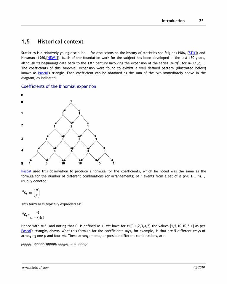
although its beginnings date back to the 13th century involving the expansion of the series (p+q)n, for n=0,1,2....

The coefficients of this 'binomial' expansion were found to exhibit a well defined pattern (illustrated below)

known as Pascal's triangle. Each coefficient can be obtained as the sum of the two immediately above in the

diagram, as indicated.

Coefficients of the Binomial expansion

Pascal used this observation to produce a formula for the coefficients, which he noted was the same as the

formula for the number of different combinations (or arrangements) of r events from a set of n (r=0,1,...n). ,

usually denoted:

or nr

nC

r

This formula is typically expanded as:

!=

( )! !n

rn

Cn r r

Hence with n=5, and noting that 0! is defined as 1, we have for r=[0,1,2,3,4,5] the values [1,5,10,10,5,1] as per

Pascal's triangle, above. What this formula for the coefficients says, for example, is that are 5 different ways of

arranging one p and four q's. These arrangements, or possible different combinations, are:

pqqqq, qpqqq, qqpqq, qqqpq, and qqqqp

Historical context26

www.statsref.com (c) 2018

and exactly the same is true if we took one q and four p's. There is only one possible arrangement of all p's or all

q's, but there are 10 possible combinations or sequences if there are 2 of one and 3 of the other. The possible

different combinations are:

ppqqq, qppqq, qqppq, qqqpp, pqpqq, pqqpq, pqqqp, qpqpq, qpqqp, qqpqp

In these examples the order of arrangement is important, and we are interested in all possible combinations. If

the order is not important the number of arrangements would be greater and the formula simplifies to counting

the number of permutations:

!=

( )!n

rn

Pn r

Assuming (p+q)=1 then clearly (p+q)n=1. Jakob Bernoulli's theorem (published in 1713, after his death) states that

if p is the probability of a single event occurring (e.g. a 2 being the result when a six-sided die is thrown), and q

=1-p is the probability of it not occurring (e.g. the die showing any other value but 2) then the probability of the

event occurring at least m times in n trials is the sum of all the terms of (p+q)n starting from the term with

elements including pr where r≥m, i.e.

!

! !

nr n r

r m

np q

r n r

So, if a die is thrown 5 times, the expected number of occasions a 2 will occur will be determined by the terms of

the binomial expansion for which p =1/6, and q =1-p = 5/6 ):

0 5 1 4 2 3 3 2 4 1 5 0,5 ,10 ,10 ,5 ,p q p q p q p q p q p q

which in this case give us the set of probabilities (to 3dp): 0.402,0.402,0.161,0.032,0.003,0.000. So the chance of

throwing at least one "2" from 5 throws of an unbiased die is the sum of all the terms from m=1 to 5, i.e. roughly

60% (59.8%), and the chances of all 5 throws turning up as a 2 is almost zero. Notice that we could also have

computed this result more directly as 1 minus the probability of no twos, which is 1-(1/6)0(5/6)5=1-0.402, the

same result as above.

This kind of computation, which is based on an a priori understanding of a problem in which the various outcomes

are equally likely, works well in certain fields, such as games of chance — roulette, card games, dice games — but

is not readily generalized to more complex and familiar problems. In most cases we do not know the exact chance

of a particular event occurring, but we can obtain an estimate of this assuming we have a fairly large and

representative sample of data. For example, if we collate data over a number of years on the age at which males

and females die in a particular city, then one might use this information to provide an estimate of the probability

that a woman of age 45 resident in that location will die within the next 12 months. This information, which is a

form of a posteriori calculation of probability, is exactly the kind of approach that forms the basis for what are

known as mortality tables, and these are used by the life insurance industry to guide the setting of insurance

premiums. Statisticians involved in this particular field are called actuaries, and their principal task is to analyze

collected data on all manner of events in order to produce probability estimates for a range of outcomes on which

insurance premiums are then based. The collected data are typically called statistics, here being the plural form.

The term statistics in the singular, refers to the science of how best to collect and analyze such data.

Introduction 27

www.statsref.com (c) 2018

Returning to the games of chance examples above, we could approach the problem of determining the probability

that at least one 2 is thrown from 5 separate throws of the die by conducting an experiment or trial. First, we

could simply throw a die 5 times and count the number of times (if any) a 2 was the uppermost face. However,

this would be a very small trial of just one set of throws. If we conducted many more trials, perhaps 1000 or

more, we would get a better picture of the pattern of events. More specifically we could make a chart of the

observed frequency of each type of event, where the possible events are: zero 2s, one 2, two 2s and so on up to

five 2s. In practice, throwing a 6-sided die a very large number of times and counting the frequency with which

each value appears is very time-consuming and difficult. Errors in the process will inevitably creep in: the physical

die used is unlikely to be perfect, in the sense that differences in the shape of its corners and surfaces may lead

some faces to be very slightly more likely to appear uppermost than others; as time goes on the die will wear, and

this could affect the results; the process of throwing a die and the surface onto which the die is thrown may

affect the results; over time we may make errors in the counting process, especially if the process continues for a

very long time... in fact there are very many reasons for arguing that a physical approach is unlikely to work well.

As an alternative we can use a simple computer program with a random number generator, to simulate the

throwing of a six-sided die. Although modern random number generators are extremely good, in that their

randomness has been the subject of an enormous amount of testing and research, there will be a very slight bias

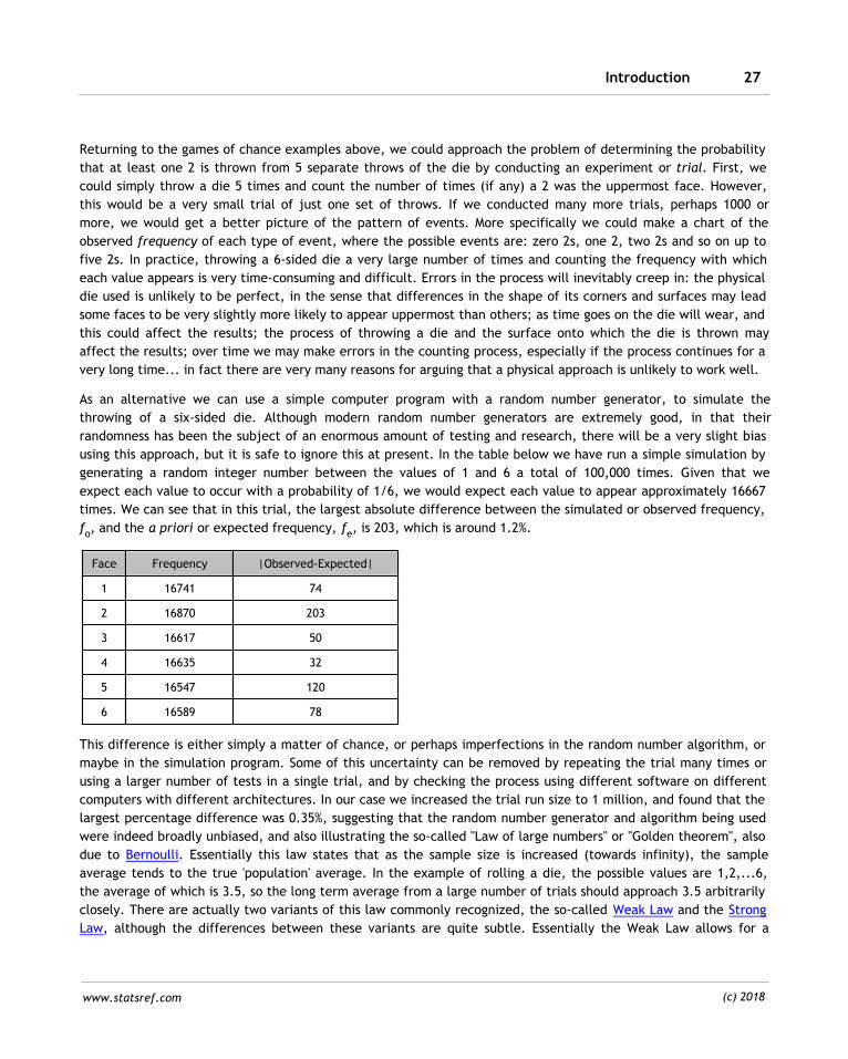
using this approach, but it is safe to ignore this at present. In the table below we have run a simple simulation by

generating a random integer number between the values of 1 and 6 a total of 100,000 times. Given that we

expect each value to occur with a probability of 1/6, we would expect each value to appear approximately 16667

times. We can see that in this trial, the largest absolute difference between the simulated or observed frequency,

fo, and the a priori or expected frequency, fe, is 203, which is around 1.2%.

Face Frequency |Observed-Expected|

1 16741 74

2 16870 203

3 16617 50

4 16635 32

5 16547 120

6 16589 78

This difference is either simply a matter of chance, or perhaps imperfections in the random number algorithm, or

maybe in the simulation program. Some of this uncertainty can be removed by repeating the trial many times or

using a larger number of tests in a single trial, and by checking the process using different software on different

computers with different architectures. In our case we increased the trial run size to 1 million, and found that the

largest percentage difference was 0.35%, suggesting that the random number generator and algorithm being used

were indeed broadly unbiased, and also illustrating the so-called "Law of large numbers" or "Golden theorem", also

due to Bernoulli. Essentially this law states that as the sample size is increased (towards infinity), the sample

average tends to the true 'population' average. In the example of rolling a die, the possible values are 1,2,...6,

the average of which is 3.5, so the long term average from a large number of trials should approach 3.5 arbitrarily

closely. There are actually two variants of this law commonly recognized, the so-called Weak Law and the Strong

Law, although the differences between these variants are quite subtle. Essentially the Weak Law allows for a

Historical context28

www.statsref.com (c) 2018

larger (possibly infinite) number of very small differences between the true average and the long term sampled

average, whilst the Strong Law allows just for a finite number of such cases.

This example has not directly told us how likely we are to see one or more 2s when the die is thrown five times. In

this case we have to simulate batches of 5 throws at a time, and count the proportion of these batches that have

one or more 2s thrown. In this case we again compute 100,000 trials, each of which involves 5 throws (so 0.5

million iterations in total) and we find the following results from a sequence of such trials: 59753, 59767,59806,...

each of which is very close to the expected value based on the percentage we derived earlier, more precisely

59812 (59.812%). In general it is unnecessary to manually or programmatically compute such probabilities for well-

known distributions such as the Binomial, since almost all statistical software packages will perform the

computation for you. For example, the Excel function BINOMDIST() could be used. Until relatively recently

statistical tables, laboriously calculated by hand or with the aid of mechanical calculators, were the principal

means of comparing observed results with standard distributions. Although this is no longer necessary the use of

tables can be a quick and simple procedure, and we have therefore included a number of these in the Resources

topic, Distribution tables section, of this Handbook.

A number of observations are worth making about the above example. First, although we are conducting a series

of trials, and using the observed data to produce our probability estimates, the values we obtain vary. So there is

a distribution of results, most of which are very close to our expected (true) value, but in a smaller number of

cases the results we obtain might, by chance, be rather more divergent from the expected frequency. This

pattern of divergence could be studied, and the proportion of trials that diverged from the expected value by

more than 1%, 2% etc. could be plotted. We could then compare an observed result, say one that diverged by 7%

from that expected, and ask "how likely is it that this difference is due to chance?". For example, if there was less

than one chance in 20 (5%) of such a large divergence, we might decide the observed value was probably not a

simple result of chance but more likely that some other factor was causing the observed variation. From the Law

of Large Numbers we now know that the size of our sample or trial is important — smaller samples diverge more

(in relative, not absolute, terms) than larger samples, so this kind of analysis must take into account sample size.

Many real-world situations involve modest sized samples and trials, which may or may not be truly representative

of the populations from which they are drawn. The subject of statistics provides specific techniques for addressing

such questions, by drawing upon experiments and mathematical analyses that have examined a large range of

commonly occurring questions and datasets.

A second observation about this example is that we have been able to compare our trials with a well-defined and

known 'true value', which is not generally the situation encountered. In most cases we have to rely more heavily

on the data and an understanding of similar experiments, in order to obtain some idea of the level of uncertainty

or error associated with our findings.

A third, and less obvious observation, is that if our trial, experiments and/or computer simulations are in some

way biased or incorrectly specified or incomplete, our results will also be of dubious value. In general it is quite

difficult to be certain that such factors have not affected the observed results and therefore great care is needed

when designing experiments or producing simulations.

Finally, it is important to recognize that a high proportion of datasets are not obtained from well-defined and

controlled experiments, but are observations made and/or collections of data obtained, by third parties, often

government agencies, with a whole host of known and unknown issues relating to their quality and how

representative they are. Similarly, much data is collected on human populations and their behavior, whether this

be medical research data, social surveys, analysis of purchasing behavior or voting intentions. Such datasets are,

Introduction 29

www.statsref.com (c) 2018

almost by definition, simply observations on samples from a population taken at a particular point in time, in

which the sampling units (individual people) are not fully understood or 'controlled' and can only loosely be

regarded as members of a well-defined 'population'.

With the explosion in the availability of scientific data during the latter part of the 18th century and early 19th

century, notably in the fields of navigation, geodesy and astronomy, efforts were made to identify associations

and patterns that could be used to simplify the datasets. The aim was to minimize the error associated with large

numbers of observations by examining the degree to which they fitted a simple model, such as a straight line or

simple curve, and then to predict the behavior of the variables or system under examination based on this

approximation. One of the first and perhaps most notable of these efforts was the discovery of the method of

Least Squares, which Gauss reputedly devised at the age of 18. This method was independently discovered and

developed by a number of other scientists, notably Legendre, and applied in a variety of different fields. In the

case of statistical analysis, least squares is most commonly encountered in connection with linear and non-linear

regression, but it was originally devised simply as the 'best' means of fitting an analytic curve (or straight line) to a

set of data, in particular measurements of astronomical orbits.

During the course of the late 1900s and the first half of the 20th century major developments were made in many

areas of statistics. A number of these are discussed in greater detail in the sections which follow, but of particular

note is the work of a series of scientists and mathematicians working at University College London (UCL). This

commenced in the 1860s with the research of the scientist Sir Francis Galton (a relation of Charles Darwin), who

was investigating whether characteristics of the human population appeared to be acquired or inherited, and if

inherited, whether humankind could be altered (improved) by selective breeding (a highly controversial scientific

discipline, known as Eugenics). The complexity of this task led Galton to develop the concepts of correlation and

regression, which were subsequently developed by Karl Pearson and refined by his student, G Udny Yule, who

delivered an influential series of annual lectures on statistics at UCL which became the foundation of his famous

book, An Introduction to the Theory of Statistics [YUL1], first published in 1911. Another student of Pearson at

UCL was a young chemist, William Gosset, who worked for the brewing business, Guinness. He is best known for

his work on testing data that have been obtained from relatively small samples. Owing to restrictions imposed by

his employers on publishing his work under his own name, he used the pseudonym "Student", from which the well-

known "Students t-test" and the t-distribution arise. Also joining UCL for 10 years as Professor of Eugenics, was R A

Fisher, perhaps the most important and influential statistician of the 20th century. Fisher's contributions were

many, but he is perhaps most famous for his work on the Design of Experiments [FIS1], a field which is central to

the conduct of controlled experiments such as agricultural and medical trials. Also at UCL, but working in a

different field, psychology, Charles Spearman was responsible for the introduction of a number of statistical

techniques including Rank Correlation and Factor Analysis. And lastly, but not least, two eminent statisticians:

Austin Bradford Hill, whose work we discuss in the section on statistics in medical research, attended Pearson's

lectures at UCL and drew on many of the ideas presented in developing his formative work on the application of

statistics to medical research; and George Box, developer of much of the subject we now refer to as industrial

statistics. Aspects of his work are included in our discussion of the Design of Experiments, especially factorial

designs.

Substantial changes to the conduct of statistical analysis have come with the rise of computers, automated

monitoring and tracking technologies (e.g. GPS, smartcard systems etc.) and the Internet. The computer has

removed the need for statistical tables and, to a large extent, the need to be able to recall and compute many of

the complex expressions used in statistical analysis. They have also enabled very large volumes of data to be

stored and analyzed, which itself presents a whole new set of challenges and opportunities. To meet some of

Historical context30

www.statsref.com (c) 2018

these, scientists such as John Tukey and others developed the concept of Exploratory Data Analysis, or "EDA",

which can be described as a set of visualization tools and exploratory methods designed to help researchers

understand large and complex datasets, picking out significant features and feature combinations for further

study. This field has become one of the most active areas of research and development in recent years, spreading

well beyond the confines of the statistical fraternity, with new techniques such as Data Mining, 3D visualizations,

Exploratory Spatio-Temporal Data Analysis (ESTDA) and a whole host of other procedures becoming widely used. A

further, equally important impact of computational power, we have already glimpsed in our discussion on games

of chance — it is possible to use computers to undertake large-scale simulations for a range of purposes, amongst

the most important of which is the generation of pseudo-probability distributions for problems for which closed

mathematical solutions are not possible or where the complexity of the constraints or environmental factors make

simulation and/or randomization approaches the only viable option.

References

[FIS1] Fisher R A (1935) The Design of Experiments. Oliver & Boyd, London

[NEW1] Newman J R (1960) The World of Mathematics. Vol 3, Part VIII Statistics and the Design of Experiments. Oliver & Boyd,

London

[STI1] Stigler S M (1986) The History of Statistics. Harvard University Press, Harvard, Mass.

[YUL1] Yule G U, Kendall M G (1950) Introduction to the Theory of Statistics. 14th edition, Charles Griffin & Co, London

MacTutor: The MacTutor History of Mathematics Archive. University of St Andrews, UK: http://www-history.mcs.st-and.ac.uk/

Mathworld: Weisstein E W "Weak Law of Large Numbers" and "Strong Law of Large Numbers":

http://mathworld.wolfram.com/WeakLawofLargeNumbers.html

Wikipedia: History of statistics: http://en.wikipedia.org/wiki/History_of_statistics

Introduction 31

www.statsref.com (c) 2018

1.6 An applications-led discipline

As mentioned in the previous section, the discipline that we now know as Statistics, developed from early work in

a number of applied fields. It was, and is, very much an applied science. Gambling was undoubtedly one of the

most important early drivers of research into probability and statistical methods and Abraham De Moivre's book,

published in 1718, "The Doctrine of Chance: A method of calculating the probabilities of events in play" [DEM1]

was essential reading for any serious gambler at the time. The book contained an explanation of the basic ideas of

probability, including permutations and combinations, together with detailed analysis of a variety of games of

chance, including card games with delightful names such as Basette and Pharaon (Faro), games of dice, roulette,

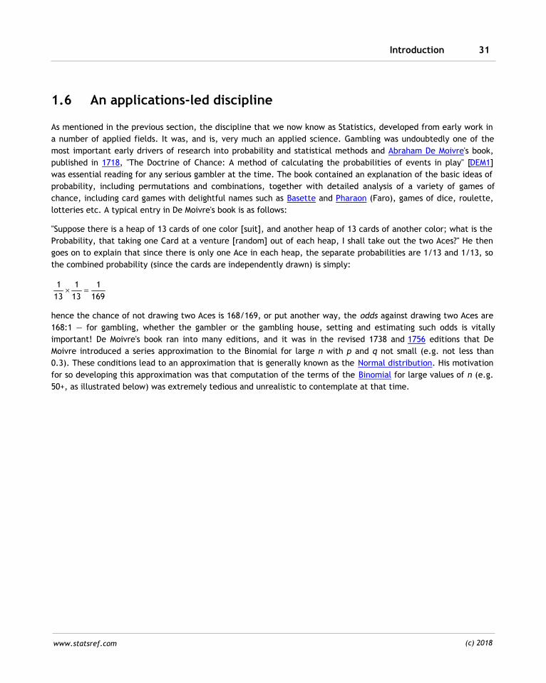
lotteries etc. A typical entry in De Moivre's book is as follows:

"Suppose there is a heap of 13 cards of one color [suit], and another heap of 13 cards of another color; what is the

Probability, that taking one Card at a venture [random] out of each heap, I shall take out the two Aces?" He then

goes on to explain that since there is only one Ace in each heap, the separate probabilities are 1/13 and 1/13, so

the combined probability (since the cards are independently drawn) is simply:

1 1 1

13 13 169

hence the chance of not drawing two Aces is 168/169, or put another way, the odds against drawing two Aces are

168:1 — for gambling, whether the gambler or the gambling house, setting and estimating such odds is vitally

important! De Moivre's book ran into many editions, and it was in the revised 1738 and 1756 editions that De

Moivre introduced a series approximation to the Binomial for large n with p and q not small (e.g. not less than

0.3). These conditions lead to an approximation that is generally known as the Normal distribution. His motivation

for so developing this approximation was that computation of the terms of the Binomial for large values of n (e.g.

50+, as illustrated below) was extremely tedious and unrealistic to contemplate at that time.

An applications-led discipline32

www.statsref.com (c) 2018

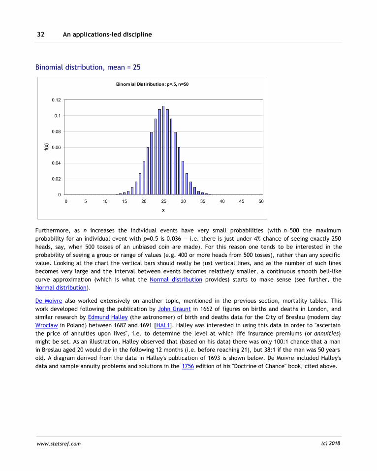
Binomial distribution, mean = 25

Binomial Distiribution: p=.5, n=50

0

0.02

0.04

0.06

0.08

0.1

0.12

0 5 10 15 20 25 30 35 40 45 50

x

f(x)

Furthermore, as n increases the individual events have very small probabilities (with n=500 the maximum

probability for an individual event with p=0.5 is 0.036 — i.e. there is just under 4% chance of seeing exactly 250

heads, say, when 500 tosses of an unbiased coin are made). For this reason one tends to be interested in the

probability of seeing a group or range of values (e.g. 400 or more heads from 500 tosses), rather than any specific

value. Looking at the chart the vertical bars should really be just vertical lines, and as the number of such lines

becomes very large and the interval between events becomes relatively smaller, a continuous smooth bell-like

curve approximation (which is what the Normal distribution provides) starts to make sense (see further, the

Normal distribution).

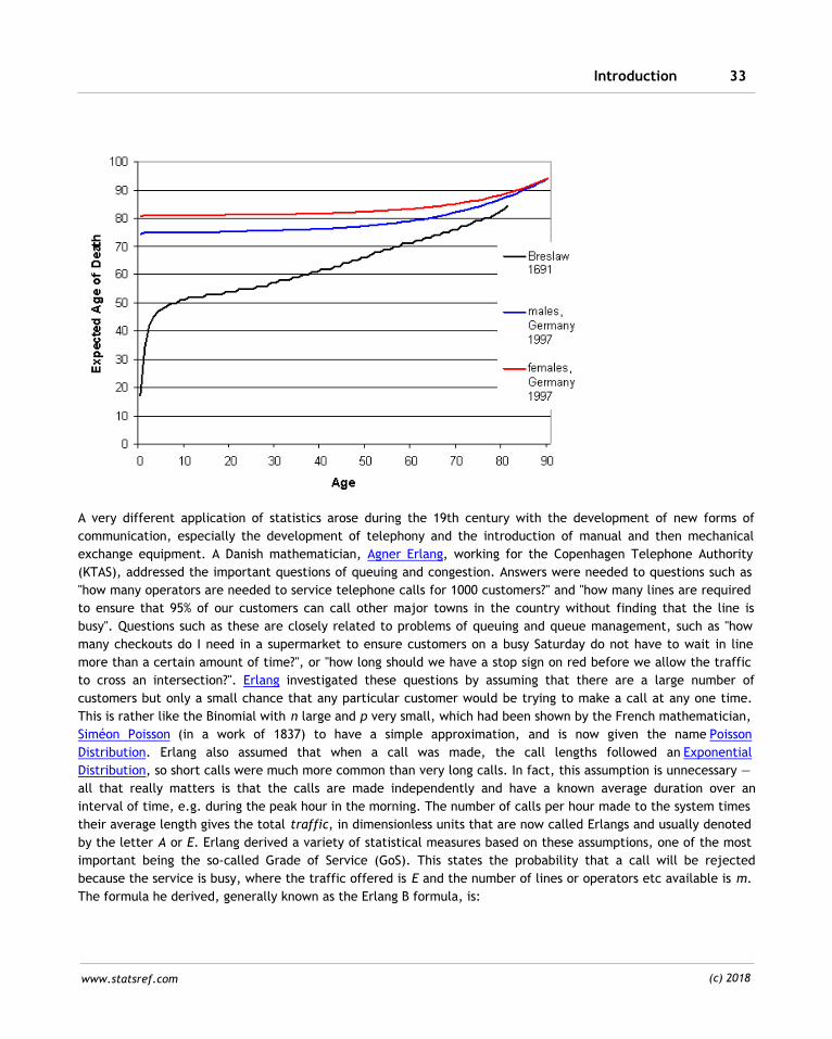
De Moivre also worked extensively on another topic, mentioned in the previous section, mortality tables. This

work developed following the publication by John Graunt in 1662 of figures on births and deaths in London, and

similar research by Edmund Halley (the astronomer) of birth and deaths data for the City of Breslau (modern day

Wrocław in Poland) between 1687 and 1691 [HAL1]. Halley was interested in using this data in order to "ascertain

the price of annuities upon lives", i.e. to determine the level at which life insurance premiums (or annuities)

might be set. As an illustration, Halley observed that (based on his data) there was only 100:1 chance that a man

in Breslau aged 20 would die in the following 12 months (i.e. before reaching 21), but 38:1 if the man was 50 years

old. A diagram derived from the data in Halley's publication of 1693 is shown below. De Moivre included Halley's

data and sample annuity problems and solutions in the 1756 edition of his "Doctrine of Chance" book, cited above.

Introduction 33

www.statsref.com (c) 2018

A very different application of statistics arose during the 19th century with the development of new forms of

communication, especially the development of telephony and the introduction of manual and then mechanical

exchange equipment. A Danish mathematician, Agner Erlang, working for the Copenhagen Telephone Authority

(KTAS), addressed the important questions of queuing and congestion. Answers were needed to questions such as

"how many operators are needed to service telephone calls for 1000 customers?" and "how many lines are required

to ensure that 95% of our customers can call other major towns in the country without finding that the line is

busy". Questions such as these are closely related to problems of queuing and queue management, such as "how

many checkouts do I need in a supermarket to ensure customers on a busy Saturday do not have to wait in line

more than a certain amount of time?", or "how long should we have a stop sign on red before we allow the traffic

to cross an intersection?". Erlang investigated these questions by assuming that there are a large number of

customers but only a small chance that any particular customer would be trying to make a call at any one time.

This is rather like the Binomial with n large and p very small, which had been shown by the French mathematician,

Siméon Poisson (in a work of 1837) to have a simple approximation, and is now given the name Poisson

Distribution. Erlang also assumed that when a call was made, the call lengths followed an Exponential

Distribution, so short calls were much more common than very long calls. In fact, this assumption is unnecessary —

all that really matters is that the calls are made independently and have a known average duration over an

interval of time, e.g. during the peak hour in the morning. The number of calls per hour made to the system times

their average length gives the total traffic, in dimensionless units that are now called Erlangs and usually denoted

by the letter A or E. Erlang derived a variety of statistical measures based on these assumptions, one of the most

important being the so-called Grade of Service (GoS). This states the probability that a call will be rejected

because the service is busy, where the traffic offered is E and the number of lines or operators etc available is m.

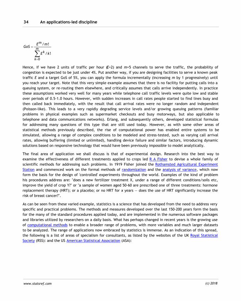
The formula he derived, generally known as the Erlang B formula, is:

An applications-led discipline34

www.statsref.com (c) 2018

0

/ !

/ !

m

mk

k

E mGoS

E k

Hence, if we have 2 units of traffic per hour (E=2) and m=5 channels to serve the traffic, the probability of

congestion is expected to be just under 4%. Put another way, if you are designing facilities to serve a known peak

traffic E and a target GoS of 5%, you can apply the formula incrementally (increasing m by 1 progressively) until

you reach your target. Note that this very simple example assumes that there is no facility for putting calls into a

queuing system, or re-routing them elsewhere, and critically assumes that calls arrive independently. In practice

these assumptions worked very well for many years while telephone call traffic levels were quite low and stable

over periods of 0.5-1.0 hours. However, with sudden increases in call rates people started to find lines busy and

then called back immediately, with the result that call arrival rates were no longer random and independent

(Poisson-like). This leads to a very rapidly degrading service levels and/or growing queuing patterns (familiar

problems in physical examples such as supermarket checkouts and busy motorways, but also applicable to

telephone and data communications networks). Erlang, and subsequently others, developed statistical formulas

for addressing many questions of this type that are still used today. However, as with some other areas of

statistical methods previously described, the rise of computational power has enabled entire systems to be

simulated, allowing a range of complex conditions to be modeled and stress-tested, such as varying call arrival

rates, allowing buffering (limited or unlimited), handling device failure and similar factors, introducing dynamic

solutions based on responsive technology that would have been previously impossible to model analytically.

The final area of application we shall discuss is that of experimental design. Research into the best way to

examine the effectiveness of different treatments applied to crops led R A Fisher to devise a whole family of

scientific methods for addressing such problems. In 1919 Fisher joined the Rothamsted Agricultural Experiment

Station and commenced work on the formal methods of randomization and the analysis of variance, which now

form the basis for the design of 'controlled' experiments throughout the world. Examples of the kind of problem

his procedures address are: "does a new fertilizer treatment X, under a range of different conditions/soils etc,

improve the yield of crop Y?" or "a sample of women aged 50-60 are prescribed one of three treatments: hormone

replacement therapy (HRT); or a placebo; or no HRT for x years — does the use of HRT significantly increase the

risk of breast cancer?".

As can be seen from these varied example, statistics is a science that has developed from the need to address very

specific and practical problems. The methods and measures developed over the last 150-200 years form the basis

for the many of the standard procedures applied today, and are implemented in the numerous software packages

and libraries utilized by researchers on a daily basis. What has perhaps changed in recent years is the growing use

of computational methods to enable a broader range of problems, with more variables and much larger datasets

to be analyzed. The range of applications now embraced by statistics is immense. As an indication of this spread,

the following is a list of areas of specialism for consultants, as listed by the websites of the UK Royal Statistical

Society (RSS): and the US American Statistical Association (ASA):

Introduction 35

www.statsref.com (c) 2018

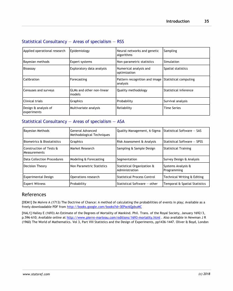
Statistical Consultancy — Areas of specialism — RSS

Applied operational research Epidemiology Neural networks and genetic

algorithms

Sampling

Bayesian methods Expert systems Non-parametric statistics Simulation

Bioassay Exploratory data analysis Numerical analysis and

optimization

Spatial statistics

Calibration Forecasting Pattern recognition and image

analysis

Statistical computing

Censuses and surveys GLMs and other non-linear

models

Quality methodology Statistical inference

Clinical trials Graphics Probability Survival analysis

Design & analysis of

experiments

Multivariate analysis Reliability Time Series

Statistical Consultancy — Areas of specialism — ASA

Bayesian Methods General Advanced

Methodological Techniques

Quality Management, 6-Sigma Statistical Software — SAS

Biometrics & Biostatistics Graphics Risk Assessment & Analysis Statistical Software — SPSS

Construction of Tests &

Measurements

Market Research Sampling & Sample Design Statistical Training

Data Collection Procedures Modeling & Forecasting Segmentation Survey Design & Analysis

Decision Theory Non Parametric Statistics Statistical Organization &

Administration

Systems Analysis &

Programming

Experimental Design Operations research Statistical Process Control Technical Writing & Editing

Expert Witness Probability Statistical Software — other Temporal & Spatial Statistics

References

[DEM1] De Moivre A (1713) The Doctrine of Chance: A method of calculating the probabilities of events in play; Available as a

freely downloadable PDF from http://books.google.com/books?id=3EPac6QpbuMC

[HAL1] Halley E (1693) An Estimate of the Degrees of Mortality of Mankind. Phil. Trans. of the Royal Society, January 1692/3,

p.596-610; Available online at http://www.pierre-marteau.com/editions/1693-mortality.html . Also available in Newman J R

(1960) The World of Mathematics. Vol 3, Part VIII Statistics and the Design of Experiments, pp1436-1447. Oliver & Boyd, London

Chapter

2

Statistical data 39

www.statsref.com (c) 2018

2 Statistical data

Statistics (plural) is the field of science that involves the collection, analysis and reporting of information that has

been sampled from the world around us. The term sampled is important here. In most instances the data we

analyze is a sample (a carefully selected representative subset) from a much larger population. In a production

process, for example, the population might be the set of integrated circuit devices produced by a specific

production line on a given day (perhaps 10,000 devices) and a sample would be a selection of a much smaller

number of devices from this population (e.g. a sample of 100, to be tested for reliability). In general this sample

should be arranged in such a way as to ensure that every chip from the population has an equal chance of being

selected. Typically this is achieved by deciding on the number of items to sample, and then using equi-probable

random numbers to choose the particular devices to be tested from the labeled population members. The details

of this sampling process, and the sample size required, is discussed in the section Sampling and sample size.

The term statistic (singular) refers to a value or quantity, such as the mean value, maximum or total, calculated

from a sample. Such values may be used to estimate the (presumed) population value of that statistic. Such

population values, particular key values such as the mean and variance, are known as parameters of the pattern

or distribution of population values.

In many instances the question of what constitutes the population is not as clear as suggested above. When

undertaking surveys of householders, the total population is rarely known, although an estimate of the population

size may be available. Likewise, when undertaking field research, taking measurements of soil contaminants, or

air pollutants or using remote sensing data, the population being investigated is often not so well-defined and may

be infinite. When examining a particular natural or man made process, the set of outcomes of the process may be

considered as the population, so the process outcomes are effectively the population.

Since statistics involves the analysis of data, and the process of obtaining data involves some kind of measurement

process, a good understanding of measurement is important. In the subsections that follow, we discuss the

question of measurement and measurement scales, and how measured data can be grouped into simple classes to

be produce data distributions. Finally we introduce two issues that serve to disguise or alter the results of

measurement in somewhat unexpected ways. The first of these is the so-called statistical grouping affect,

whereby grouped data produce results that differ from ungrouped data in a non-obvious manner. The second of

these is a spatial effect, whereby selection of particular arrangement of spatial groupings (such as census

districts) can radically alter the results one obtains.

Perhaps one of the mostly hotly debated topics in recent years has been the rise of so-called "Big Data". In an

article "Big Data: Are we making a big mistake?" in the Financial Times, March 2014, Tim Harford addresses these

issues and more, highlighting some of the less obvious issues posed by Big Data. Perhaps primary amongst these is

the bias that is found in many such datasets. Such biases may be subtle and difficult to identify and impossible to

manage. For example, almost all Internet-related Big Data is intrinsically biased in favor of those who have access

to and utilize the Internet most, with demographic and geographic bias built-in. The same applies for specific

services, such as Google, Twitter, Facebook, mobile phone networks, opt-in online surveys, opt-in emails — the

examples are many and varied, but the problems are much the same as those familiar to statisticians for over a

century. Big Data does not imply good data or unbiased data, and Big Data presents other problems — it is all to

easy to focus on the data exploration and pattern discovery, identifying correlations that may well be spurious — a

result of the sheer volume of data and the number of events and variables measured. With enough data and

40

www.statsref.com (c) 2018

enough comparisons, statistically significant findings are inevitable, but that does not necessarily provide real

insights, understanding, or identification of causal relationships. Of course there are many important and

interesting datasets where the collection and storage is far more systematic, less subject to bias, recording

variables in a direct manner, with 'complete' and 'clean' records. Such data are stored and managed well and tend

to be those collected by agencies who supplement the data with metadata (data about data) and quality

assurance information.

Measurement

In principle the process of measurement should seek to ensure that results obtained are consistent, accurate (a

term that requires separate discussion), representative, and if necessary independently reproducible. Some

factors of particular importance include:

· framework — the process of producing measurements is both a technical and, to an extent, philosophical

exercise. The technical framework involves the set of tools and procedures used to obtain and store numerical

data regarding the entities being measured. Different technical frameworks may produce different data of

varying quality from the same set of entities. In many instances measurement is made relative to some

internationally agreed standard, such as the meter (for length) or the kilogram (for mass). The philosophical

framework involves the notion that a meaningful numerical value or set of values can be assigned (using some

technical framework) to attributes of the entities. This is a model or representation of these entity attributes in

the form of numerical data — a person's height is an attribute that we can observe visually, describe in words,

or assign a number to based on an agreed procedure relative to a standard (in meters, which in turn is based on

the agreed measurement of the speed of light in a vacuum)

· observer effects — in both social and pure science research, observer effects can be significant. As a simple

example, if we are interested in measuring the temperature and air quality in a process clean room, the

presence of a person taking such measurements would inevitably have some affect on the readings. Similarly, in

social research many programmes can display the so-called Hawthorne Effect in which changes (often

improvements) in performance are partially or wholly the result of behavioral changes in the presence of the

observer (reflecting greater interest in the individuals being observed)

· metrics — when measuring distance in the plane using Euclidean measure the results are invariant under

translation, reflection and rotation. So if we use Euclidean measure we can safely make measurements of

distances over relatively small areas and not worry about the location or orientation at which we took the

measurements and made the calculation. However, over larger areas and/or using a different metric,

measurements may fail the invariance test. In the case of measurements that seek to compute distances,

measurements made using the so-called City block or Manhattan distance are not invariant under rotation.

Likewise, Euclidean distance measurements give incorrect results over larger distances on the Earth's surface

(e.g. >20 kilometers). When making other forms of measurement similar issues apply (e.g. the effect of the

local gravitational field on weight, the local magnetic field on magnetic flux, etc.)

· temporal effects — measurement made at different times of the day, days of the year and in different years

will inevitably differ. If the differences are simply random fluctuations in a broadly constant process (results are

unaffected by temporal translation of the data) the process is described as being stationary. If a trend exists

(which could be linear, cyclical or some other pattern) the process is said to be non-stationary. All too often

consideration of the temporal aspect of measurement is omitted, e.g. a person's height will be measured as

shorter in the evening as compared with the morning, a persons academic or sporting achievement can be

significantly affected by when they were born (see Gladwell, 2008, for an extensive discussion of this issue,

Statistical data 41

www.statsref.com (c) 2018

[GLA1]) — the issue is always present even if it is not of direct concern. Frequently the sequence of event

measurement is important, especially where humans are doing the measurements or recordings, since issues

such as concentration become important over time; event sequences may also be explicitly monitored, as in

control charts, time series analysis and neural network learning

· spatial effects — measurements made at different locations will typically exhibit spatial variation. If all

locations provided identical data the results would be a spatially uniform distribution. If the results are similar

in all directions at all locations, then the process is described as isotropic (i.e. results are rotationally

invariant). If the results are similar at all locations (i.e. the results are translationally invariant) then the

process can be described as stationary. In practice most spatial datasets are non-stationary

Measurement scales

Measurement gives rise to values, such as counts, sets of decimal values, binary responses (yes/no,

presence/absence) etc., which may be of different types (scales). The principal scales encountered are:

· Nominal (or Categorical): data is really just assignment to named classes, such as Red, Blue, Green — or Utah,

Nevada, New York. An attribute is nominal if it successfully distinguishes between groups, but without any

implied ranking or potential for arithmetic. For example, a telephone number can be a useful attribute of a

place, but the number itself generally has no numeric meaning. It would make no sense to add or divide

telephone numbers, and there is no sense in which the number 9680244 is more or better than the number

8938049. Likewise, assigning arbitrary numerical values to classes of land type, e.g. 1=arable, 2=woodland,

3=marsh, 4=other is simply a convenient form of naming (the values are still nominal)

· Ordinal: this term refers to data values that involves a concept of order, from least to greatest and may include

negative numbers and 0. A set of apparently ordered categories such as: 1=low, 2=medium, 3=high, 4="don't

know" does not form an ordinal scale. An attribute is ordinal if it implies a ranking, in the sense that Class 1 may

be better than Class 2, but as with nominal attributes arithmetic operations do not make sense, and there is no

implication that Class 3 is worse than Class 2 by the precise amount by which Class 2 is worse than Class 1. An

example of an ordinal scale might be preferred locations for residences — an individual may prefer some areas

of a city to others, but such differences between areas may be barely noticeable or quite profound. Analysis of

nominal and ordinal data is often qualitative, or uses visualization techniques to highlight interesting patterns,

and may use non-parametric statistical methods especially when count data are available

· Interval: numeric data that exhibits order, plus the ability to measure the interval (distance) between any pair

of objects on the scale (e.g. 2x-xº3x-2x). Data are of interval type if differences make sense, as they do for

example with measurements of temperature on the Celsius or Fahrenheit scales

· Ratio: interval plus a natural origin, e.g. temperature in degrees Kelvin, weights of people (i.e. so x=2y is

meaningful); Interval or ratio scales are required for most forms of (parametric) statistical analysis. Data are

ratio scaled if it makes sense to divide one measurement by another. For example, it makes sense to say that

one person weighs twice as much as another person, but it makes no sense to say that a temperature of 20

Celsius is twice as warm as a temperature of 10 Celsius, because while weight has a meaningful absolute zero

Celsius temperature does not (but on an absolute scale of temperature, such as the Kelvin scale, 200 degrees

can indeed be said to be twice as warm as 100 degrees). It follows that negative values cannot exist on a ratio

scale.

· Cyclic: modulo data — like angles and clock time. Measurements of attributes that represent directions or cyclic

phenomena have the awkward property that two distinct points on the scale can be equal — for example, 0 and

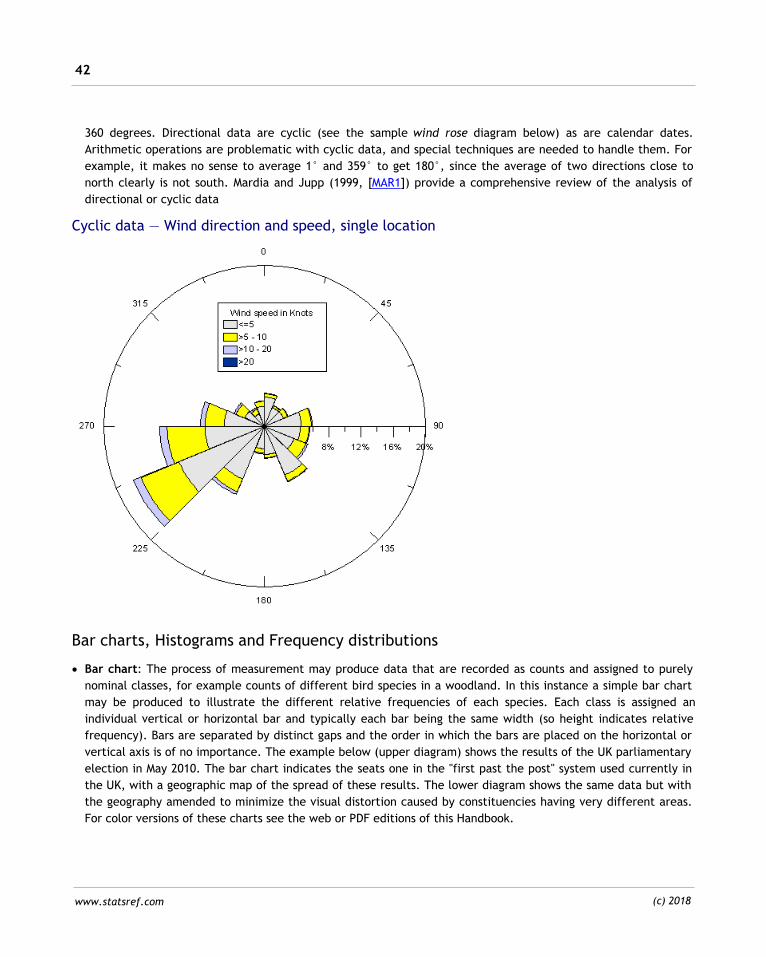
42

www.statsref.com (c) 2018

360 degrees. Directional data are cyclic (see the sample wind rose diagram below) as are calendar dates.

Arithmetic operations are problematic with cyclic data, and special techniques are needed to handle them. For

example, it makes no sense to average 1° and 359° to get 180°, since the average of two directions close to

north clearly is not south. Mardia and Jupp (1999, [MAR1]) provide a comprehensive review of the analysis of

directional or cyclic data

Cyclic data — Wind direction and speed, single location

Bar charts, Histograms and Frequency distributions

· Bar chart: The process of measurement may produce data that are recorded as counts and assigned to purely

nominal classes, for example counts of different bird species in a woodland. In this instance a simple bar chart

may be produced to illustrate the different relative frequencies of each species. Each class is assigned an

individual vertical or horizontal bar and typically each bar being the same width (so height indicates relative

frequency). Bars are separated by distinct gaps and the order in which the bars are placed on the horizontal or

vertical axis is of no importance. The example below (upper diagram) shows the results of the UK parliamentary

election in May 2010. The bar chart indicates the seats one in the "first past the post" system used currently in

the UK, with a geographic map of the spread of these results. The lower diagram shows the same data but with

the geography amended to minimize the visual distortion caused by constituencies having very different areas.

For color versions of these charts see the web or PDF editions of this Handbook.

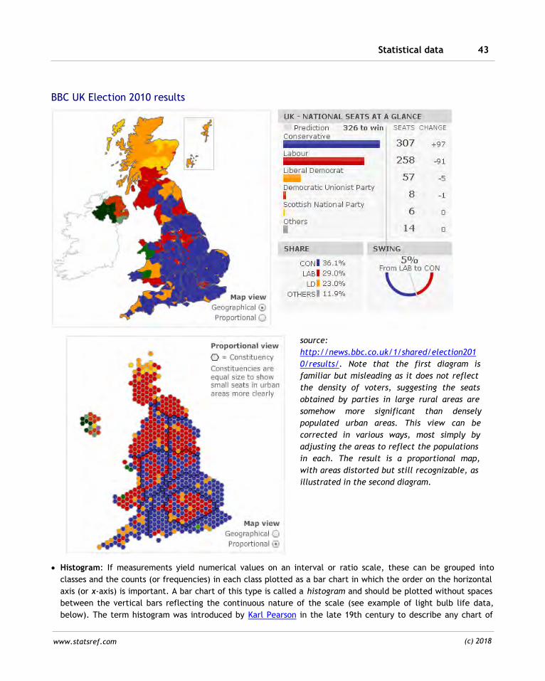
Statistical data 43

www.statsref.com (c) 2018

BBC UK Election 2010 results

source:

http://news.bbc.co.uk/1/shared/election201

0/results/. Note that the first diagram is

familiar but misleading as it does not reflect

the density of voters, suggesting the seats

obtained by parties in large rural areas are

somehow more significant than densely

populated urban areas. This view can be

corrected in various ways, most simply by

adjusting the areas to reflect the populations

in each. The result is a proportional map,

with areas distorted but still recognizable, as

illustrated in the second diagram.

· Histogram: If measurements yield numerical values on an interval or ratio scale, these can be grouped into

classes and the counts (or frequencies) in each class plotted as a bar chart in which the order on the horizontal

axis (or x-axis) is important. A bar chart of this type is called a histogram and should be plotted without spaces

between the vertical bars reflecting the continuous nature of the scale (see example of light bulb life data,

below). The term histogram was introduced by Karl Pearson in the late 19th century to describe any chart of

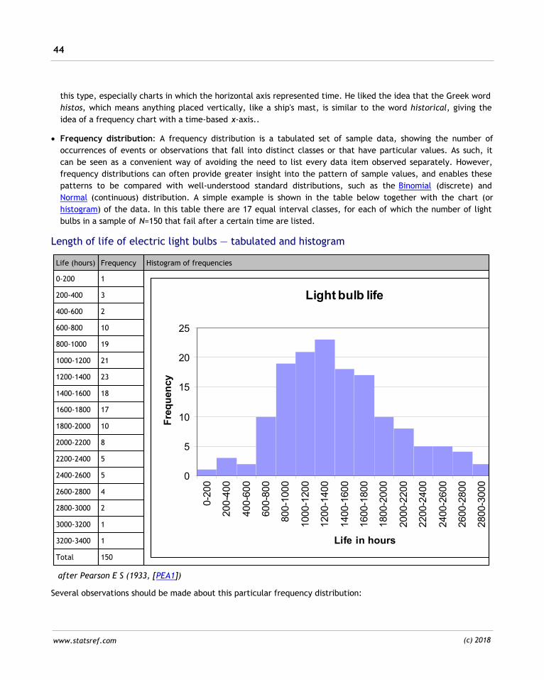
44

www.statsref.com (c) 2018

this type, especially charts in which the horizontal axis represented time. He liked the idea that the Greek word

histos, which means anything placed vertically, like a ship's mast, is similar to the word historical, giving the

idea of a frequency chart with a time-based x-axis..

· Frequency distribution: A frequency distribution is a tabulated set of sample data, showing the number of

occurrences of events or observations that fall into distinct classes or that have particular values. As such, it

can be seen as a convenient way of avoiding the need to list every data item observed separately. However,

frequency distributions can often provide greater insight into the pattern of sample values, and enables these

patterns to be compared with well-understood standard distributions, such as the Binomial (discrete) and

Normal (continuous) distribution. A simple example is shown in the table below together with the chart (or

histogram) of the data. In this table there are 17 equal interval classes, for each of which the number of light

bulbs in a sample of N=150 that fail after a certain time are listed.

Length of life of electric light bulbs — tabulated and histogram

Life (hours) Frequency Histogram of frequencies

0-200 1

Light bulb life

0

5

10

15

20

25

0-2

00

200-4

00

400-6

00

600-8

00

800-1

000

1000-1

200

1200-1

400

1400-1

600

1600-1

800

1800-2

000

2000-2

200

2200-2

400

2400-2

600

2600-2

800

2800-3

000

3000-3

200

3200-3

400

Life in hours

Fre

qu

en

cy

200-400 3

400-600 2

600-800 10

800-1000 19

1000-1200 21

1200-1400 23

1400-1600 18

1600-1800 17

1800-2000 10

2000-2200 8

2200-2400 5

2400-2600 5

2600-2800 4

2800-3000 2

3000-3200 1

3200-3400 1

Total 150

after Pearson E S (1933, [PEA1])

Several observations should be made about this particular frequency distribution:

Statistical data 45

www.statsref.com (c) 2018

(i) it has a single category or class containing the most frequent bulb life (1200-1400hrs) — this category is called

the mode, and because there is a single mode, the distribution is said to be unimodal

(ii) the set of classes in the tabulated list are not really correctly defined — the boundaries are indeterminate, and

should be specified as [0,199.9],[200-399.9], etc (or similar) or better still [0,<200], [200,<400] etc (in Pearson's

paper, which was primarily concerned with production control and sampling, he actually only supplied the

frequency diagram, not the tabulated data) — the precise definition of the boundaries of classes avoids the

problem of deciding how to assign values that lie on the boundary (e.g. a bulb with measured lifespan of exactly

200 hours)

(iii) each class is the same width (duration) and every data value is allocated to a unique class; however, when

performing certain calculations, such as computing the mean value, a decision has to be made as to whether to

use the recorded frequencies in the various classes or bins, or the source data (if available). If the frequencies

have to be used, it is necessary to define a representative value for each interval, which is usually taken to be the

mid-interval value. Note that this assumption hides the within-class variation in values which may create some

errors in computations, especially if the class widths are large. The question of bin selection is discussed later in

this section

(iv) the width (duration) of each class is somewhat arbitrary and this choice significantly affects the form of the

frequency distribution. If the class width was very small (1 hour say) most classes would contain the frequency 0,

and a few would contain just 1 failure. At the opposite extreme, if the class width was 3400 hours all the results

would be in just the one class. In both these examples very little information would be gained from inspecting the

pattern of frequencies. Selecting the class boundaries and number of classes is an important operation — it should

ensure that the minimum of information is lost, whilst also ensuring that the distribution communicates useful and

relevant information. Many authors recommend the use of an odd number of classes, and there are a myriad of

rules-of-thumb for choosing the number of classes and class boundaries (see Class Intervals, below)

(v) all the data fits into the classes (in this example). This is often not possible to achieve with equal interval

classes, especially at the upper and lower ends of the distribution. Indeed, frequency distributions with very long

tails are common, and often the final category is taken as 3000+ for example

(vi) the data being analyzed in this example can be regarded as a continuous variable (lifespan of the bulb) and is

a single variable (i.e. univariate data)

There are several extensions and variations that can be applied to the above model. The first is to rescale the

vertical axis by dividing each class value by the total sample size (N=150), in which case the data are described as

relative frequencies, and in examples such as this, the values can be considered as estimated probabilities.

A second important variant is the extension of the frequency table and chart to multivariate and multi-

dimensional cases. In the bivariate case the data may simply be separate measures applied to the same classes, or

they may be joint measures. For example, suppose that our classes show the heights of individuals in a large

representative sample. The first column of a bivariate frequency tabulation might show the frequency distribution

for men over 18 years, whilst the second column shows the same data but for women. However, if the mix of

those sampled included fathers and sons, one could construct a two-way or joint frequency distribution (or cross-

tabulation) of the men with classes "Tall" and "Short", where Tall is taken as over some agreed height. The table

below illustrates such a cross-tabulation, based on a study of families carried out by Karl Pearson and Dr Alice Lee

from 1893 onwards:

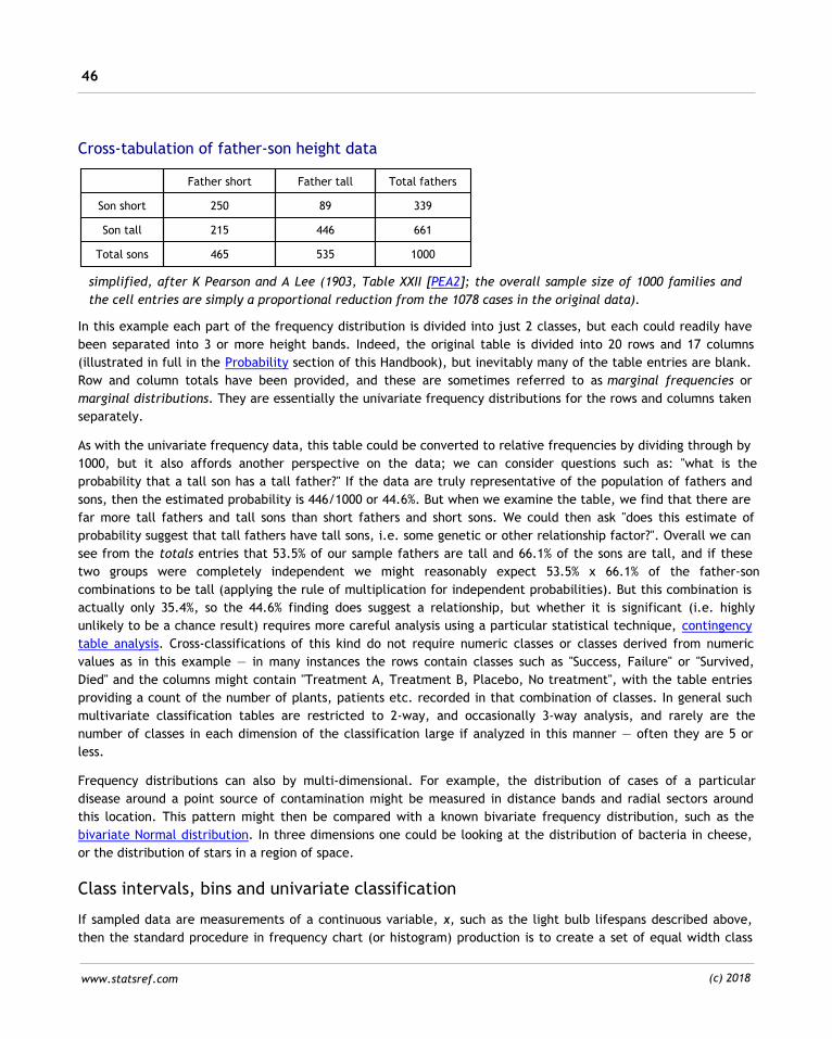
46

www.statsref.com (c) 2018

Cross-tabulation of father-son height data

Father short Father tall Total fathers

Son short 250 89 339

Son tall 215 446 661

Total sons 465 535 1000

simplified, after K Pearson and A Lee (1903, Table XXII [PEA2]; the overall sample size of 1000 families and

the cell entries are simply a proportional reduction from the 1078 cases in the original data).

In this example each part of the frequency distribution is divided into just 2 classes, but each could readily have

been separated into 3 or more height bands. Indeed, the original table is divided into 20 rows and 17 columns

(illustrated in full in the Probability section of this Handbook), but inevitably many of the table entries are blank.

Row and column totals have been provided, and these are sometimes referred to as marginal frequencies or

marginal distributions. They are essentially the univariate frequency distributions for the rows and columns taken

separately.

As with the univariate frequency data, this table could be converted to relative frequencies by dividing through by

1000, but it also affords another perspective on the data; we can consider questions such as: "what is the

probability that a tall son has a tall father?" If the data are truly representative of the population of fathers and

sons, then the estimated probability is 446/1000 or 44.6%. But when we examine the table, we find that there are

far more tall fathers and tall sons than short fathers and short sons. We could then ask "does this estimate of

probability suggest that tall fathers have tall sons, i.e. some genetic or other relationship factor?". Overall we can

see from the totals entries that 53.5% of our sample fathers are tall and 66.1% of the sons are tall, and if these

two groups were completely independent we might reasonably expect 53.5% x 66.1% of the father-son

combinations to be tall (applying the rule of multiplication for independent probabilities). But this combination is

actually only 35.4%, so the 44.6% finding does suggest a relationship, but whether it is significant (i.e. highly

unlikely to be a chance result) requires more careful analysis using a particular statistical technique, contingency

table analysis. Cross-classifications of this kind do not require numeric classes or classes derived from numeric

values as in this example — in many instances the rows contain classes such as "Success, Failure" or "Survived,

Died" and the columns might contain "Treatment A, Treatment B, Placebo, No treatment", with the table entries

providing a count of the number of plants, patients etc. recorded in that combination of classes. In general such

multivariate classification tables are restricted to 2-way, and occasionally 3-way analysis, and rarely are the

number of classes in each dimension of the classification large if analyzed in this manner — often they are 5 or

less.

Frequency distributions can also by multi-dimensional. For example, the distribution of cases of a particular

disease around a point source of contamination might be measured in distance bands and radial sectors around

this location. This pattern might then be compared with a known bivariate frequency distribution, such as the

bivariate Normal distribution. In three dimensions one could be looking at the distribution of bacteria in cheese,

or the distribution of stars in a region of space.

Class intervals, bins and univariate classification

If sampled data are measurements of a continuous variable, x, such as the light bulb lifespans described above,

then the standard procedure in frequency chart (or histogram) production is to create a set of equal width class

Statistical data 47

www.statsref.com (c) 2018

intervals (or bins) and count the frequencies occurring in each interval. The values at which the bins are

separated are often referred to as cut-points. The number of intervals to be used is a matter for the researcher to

determine, depending on the problem requirements. It is often helped, in interactive software packages, by

viewing a display of the resulting histogram as different options are selected. For visualization purposes it is

desirable to limit the number of classes to between 5 or 9, as using large numbers of classes (20+) can be difficult

to display and interpret with clarity, and an odd number of intervals will ensure there is a central class. On the

other hand, with a large set of observations that exhibit considerable spread across the range, a larger number of

classes may be more helpful and will avoid the problem of having much of the real variation hidden by large class

intervals.

There are several rules of thumb for determining the ideal number of bins and/or the width for fixed-width bins

for real-valued continuous data. These include the following (n is the number of observations or data items to be

grouped, k is the number of classes, h is the bin width, s is the standardized average spread or standard deviation

of the sample data):

max min max min, or k h

h k

These options use the range and a pre-selected bin width to define the number of bins, k, or alternatively the

number of bins is specified and the range used to determine the bin width, h. Note that if the distribution has a

very long tail, e.g. a few data items that are very much larger or smaller than all the others, these formulas will

produce excessively wide bins.

The next formula is due to Scott (1979, [SCO1]) and uses the standard deviation of the dataset, s, rather than the

range to determine bin width:

1/33.5 /h s n

Thus for 1000 data items with a standard deviation of 25, h=9. The number of bins still remains to be chosen, and

this will be a matter of choice again, but could safely use the range calculation for k, above, in most cases. Scott's

model is built on an analysis of the optimal properties of a binning arrangement with constant bin widths and an

examination of the ideas of so-called kernel density estimation (KDE) techniques. The latter use all the data

points to create a smooth estimated probability distribution (or probability density function), which has been

shown to produce excellent results but may require a considerable amount of data processing.

As mentioned earlier, if the frequencies are to be used in computations it is necessary to define a representative

value for each interval, which is usually taken to be the mid-interval value. Thus if the bin width is h, and the

mid-interval value is xi, the interval has a range from xi-h/2 to xi+h/2. This assumption hides the within-interval

variation in values which may create some errors in computations, especially if the class width are large. The so-

called Sheppard's correction, named after its author William Sheppard (1897), is an adjustment to estimates of the

variance when (Normally distributed) fixed width bins are used. Without correction the computations tend to

over-estimate the variance since they effectively treat all values in a range as the same as the mid-value.

Sheppard's correction to the variance is -h2/12, an amount that is the variance of the Uniform distribution defined

over an interval of width, h.

48

www.statsref.com (c) 2018

The table below provides details of a number of univariate classification schemes together with comments on their

use. Such schemes are essentially a generalization of fixed-width binning. Many statistical software packages

provide classification options of the types listed, although some (such as the box, Jenks and percentile methods)

are only available in a limited number of software tools.

The scheme described in the table as Natural breaks or Jenks' method is an automated procedure utilizing the

following algorithm:

Step 1: The user selects the attribute, x, to be classified and specifies the number of classes required, k

Step 2: A set of k-1 random or uniform values are generated in the range [min{x},max{x}]. These are used as initial

class boundaries or 'cut points'

Step 3: The mean values for each initial class are computed and the sum of squared deviations of class members

from the mean values is computed. The total sum of squared deviations (TSSD) is recorded

Step 4: Individual values in each class are then systematically assigned to adjacent classes by adjusting the class

boundaries to see if the TSSD can be reduced. This is an iterative process, which ends when improvement in TSSD

falls below a threshold level, i.e. when the within class variance is as small as possible and between class variance

is as large as possible. True optimization is not assured. The entire process can be optionally repeated from Step 1

or 2 and TSSD values compared

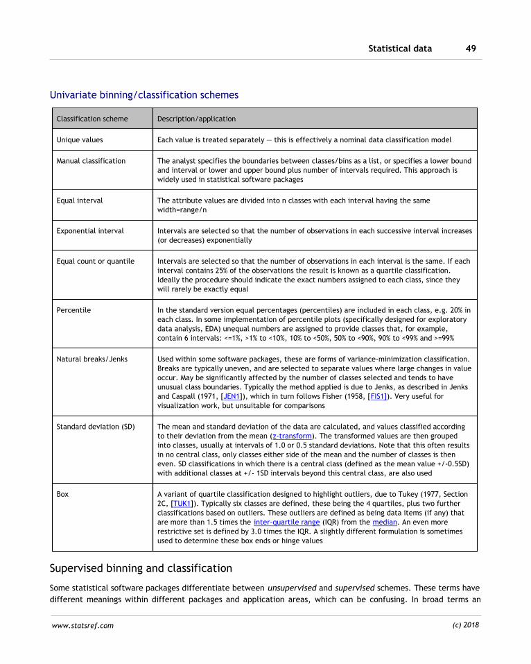
Statistical data 49

www.statsref.com (c) 2018

Univariate binning/classification schemes

Classification scheme Description/application

Unique values Each value is treated separately — this is effectively a nominal data classification model

Manual classification The analyst specifies the boundaries between classes/bins as a list, or specifies a lower bound

and interval or lower and upper bound plus number of intervals required. This approach is

widely used in statistical software packages

Equal interval The attribute values are divided into n classes with each interval having the same

width=range/n

Exponential interval Intervals are selected so that the number of observations in each successive interval increases

(or decreases) exponentially

Equal count or quantile Intervals are selected so that the number of observations in each interval is the same. If each

interval contains 25% of the observations the result is known as a quartile classification.

Ideally the procedure should indicate the exact numbers assigned to each class, since they

will rarely be exactly equal

Percentile In the standard version equal percentages (percentiles) are included in each class, e.g. 20% in

each class. In some implementation of percentile plots (specifically designed for exploratory

data analysis, EDA) unequal numbers are assigned to provide classes that, for example,

contain 6 intervals: <=1%, >1% to <10%, 10% to <50%, 50% to <90%, 90% to <99% and >=99%

Natural breaks/Jenks Used within some software packages, these are forms of variance-minimization classification.

Breaks are typically uneven, and are selected to separate values where large changes in value

occur. May be significantly affected by the number of classes selected and tends to have

unusual class boundaries. Typically the method applied is due to Jenks, as described in Jenks

and Caspall (1971, [JEN1]), which in turn follows Fisher (1958, [FIS1]). Very useful for

visualization work, but unsuitable for comparisons

Standard deviation (SD) The mean and standard deviation of the data are calculated, and values classified according

to their deviation from the mean (z-transform). The transformed values are then grouped

into classes, usually at intervals of 1.0 or 0.5 standard deviations. Note that this often results

in no central class, only classes either side of the mean and the number of classes is then

even. SD classifications in which there is a central class (defined as the mean value +/-0.5SD)

with additional classes at +/- 1SD intervals beyond this central class, are also used

Box A variant of quartile classification designed to highlight outliers, due to Tukey (1977, Section

2C, [TUK1]). Typically six classes are defined, these being the 4 quartiles, plus two further

classifications based on outliers. These outliers are defined as being data items (if any) that

are more than 1.5 times the inter-quartile range (IQR) from the median. An even more

restrictive set is defined by 3.0 times the IQR. A slightly different formulation is sometimes

used to determine these box ends or hinge values

Supervised binning and classification

Some statistical software packages differentiate between unsupervised and supervised schemes. These terms have

different meanings within different packages and application areas, which can be confusing. In broad terms an

50

www.statsref.com (c) 2018

unsupervised method utilizes the data directly, whereas a supervised method cross-refers the sample data to some

other dataset that is already divided into a number of distinct classes or categories. It then uses this other dataset

to guide (or supervise) the classification process.

In SPSS, for example, supervised (or optimal) binning refers to a procedure in which the source data is divided

into bins using cut-points that seek to minimize the mix of a separate, but linked, nominal variable in each bin.

For example, the variable to be binned might be household income in $000s p.a., and the supervisor or control

variable might be the level of education achieved by the main earner of the household. The principal technique

used, known as MDLP, starts by placing every (sorted) data item (observation) into a single large bin. The bin is

then divided using cut-points, and the mix of the linked nominal variable in each bin is examined (using an

Entropy or Diversity statistic). If every entry in the bin has the same linked nominal category then the Entropy

measure will be 0, which is regarded as optimal with respect to the nominal variable. On the other hand if there is

a large mix of nominal variables represented, of roughly equal numbers, the bin will have a higher Entropy score.

The algorithm adjusts the cut points and increases the number of cut points (and hence bins) to achieve an

improvement in the total Entropy of the binning process.

In remote-sensing applications (for example, multi-spectral satellite imagery) the task is to classify individual

image pixels into groups, which may be pre-defined (e.g. land use categories, such as Forest, Grasslands,

Buildings, Water etc) or derived from the data. Unsupervised classification in this instance refers to the use of

wholly automated procedures, such as K-means clustering, in order to group similar pixels. Supervised

classification refers to a multi-stage process, in which the dataset is compared to a reference dataset that has

already been classified, and the similarity between pixels in the dataset to be classified and the reference set is

used as a means for achieving the 'best' classification. Clearly procedures such as this, which arise in a number of

disciplines, essentially belong in the realm of multivariate data classification, which may or may not use statistical

techniques and measures as part of that process.

Scale and arrangement

In the preceding subsections we have seen that determining the ideal number and size of bins can be a quite

complicated exercise. It was noted that with too many bins only frequencies of 1 and 0 would be recorded,

whereas with very few bins, almost all the variation in the data would be hidden within the bin, or class, with

little or no variation detectable between classes. This is often the exact opposite of the ideal classification or

grouping schemes, where the aim is generally to minimize within-class variance as compared to between class

variance — making sure that classes or groupings are as homogeneous as possible. Two additional, and somewhat

unexpected factors, come into play when such groupings are made. These are known as the statistical effect and

the arrangement effect.

To understand the statistical effect (which is a scale or grouping effect) look at the regional employment statistics

shown in the Table below (after de Smith et al. (2018, [DES1]). Areas A and B both contain a total of 100,000

people who are classified as either employed or not. In area A 10% of both Europeans and Asians are unemployed

(i.e. equal proportions), and likewise in Area B we have equal proportions (this time 20% unemployed). So we

expect that combining areas A and B will give us 200,000 people, with an equal proportion of Europeans and Asians

unemployed (we would guess this to be 15%), but it is not the case — 13.6% of Europeans and 18.3% of Asians are

seen to be unemployed! The reason for this unexpected result is that in Area A there are many more Europeans

than Asians, so we are working from different total populations.

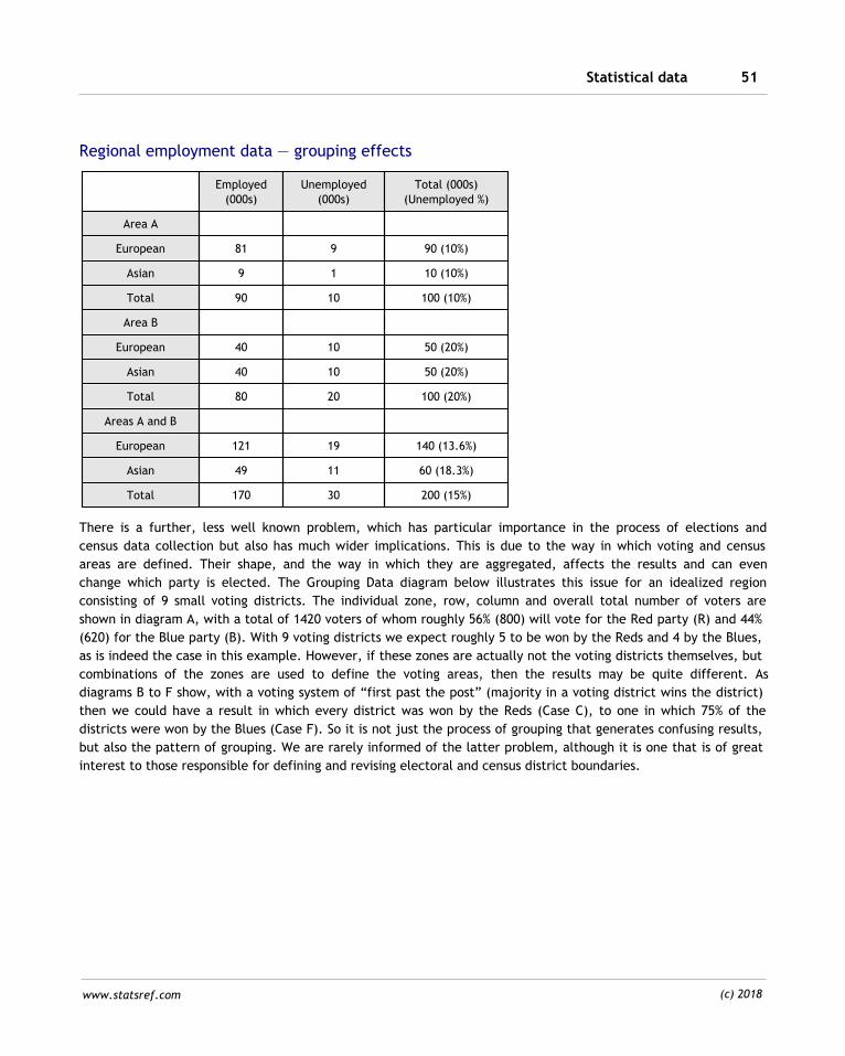
Statistical data 51

www.statsref.com (c) 2018

Regional employment data — grouping effects

Employed

(000s)

Unemployed

(000s)

Total (000s)

(Unemployed %)

Area A

European 81 9 90 (10%)

Asian 9 1 10 (10%)

Total 90 10 100 (10%)

Area B

European 40 10 50 (20%)

Asian 40 10 50 (20%)

Total 80 20 100 (20%)

Areas A and B

European 121 19 140 (13.6%)

Asian 49 11 60 (18.3%)

Total 170 30 200 (15%)

There is a further, less well known problem, which has particular importance in the process of elections and

census data collection but also has much wider implications. This is due to the way in which voting and census

areas are defined. Their shape, and the way in which they are aggregated, affects the results and can even

change which party is elected. The Grouping Data diagram below illustrates this issue for an idealized region

consisting of 9 small voting districts. The individual zone, row, column and overall total number of voters are

shown in diagram A, with a total of 1420 voters of whom roughly 56% (800) will vote for the Red party (R) and 44%

(620) for the Blue party (B). With 9 voting districts we expect roughly 5 to be won by the Reds and 4 by the Blues,

as is indeed the case in this example. However, if these zones are actually not the voting districts themselves, but

combinations of the zones are used to define the voting areas, then the results may be quite different. As

diagrams B to F show, with a voting system of “first past the post” (majority in a voting district wins the district)

then we could have a result in which every district was won by the Reds (Case C), to one in which 75% of the

districts were won by the Blues (Case F). So it is not just the process of grouping that generates confusing results,

but also the pattern of grouping. We are rarely informed of the latter problem, although it is one that is of great

interest to those responsible for defining and revising electoral and census district boundaries.

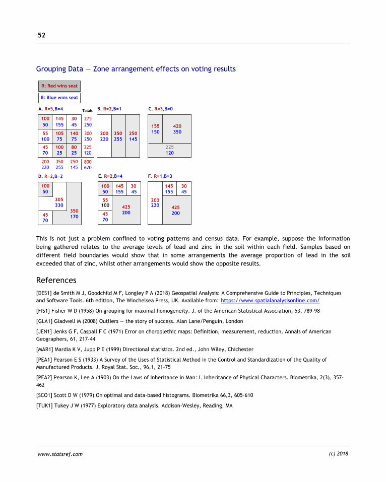
52

www.statsref.com (c) 2018

Grouping Data — Zone arrangement effects on voting results

100

50

200220

155150

10050

200220

145

155

30

45

55100

10575

14075

4570

10025

8025

350255

250145

420350

225120

305330

35017045

70

145155

3045

10050

55100

4570

425200

425200

145155

3045

200220

350255

250145

275

250

300250

225120

A. R=5,B=4 B. R=2,B=1 C. R=3,B=0

D. R=2,B=2 E. R=2,B=4 F. R=1,B=3

800620

Totals

B: Blue wins seat

R: Red wins seat

This is not just a problem confined to voting patterns and census data. For example, suppose the information

being gathered relates to the average levels of lead and zinc in the soil within each field. Samples based on

different field boundaries would show that in some arrangements the average proportion of lead in the soil

exceeded that of zinc, whilst other arrangements would show the opposite results.

References

[DES1] de Smith M J, Goodchild M F, Longley P A (2018) Geospatial Analysis: A Comprehensive Guide to Principles, Techniques

and Software Tools. 6th edition, The Winchelsea Press, UK. Available from: https://www.spatialanalysisonline.com/

[FIS1] Fisher W D (1958) On grouping for maximal homogeneity. J. of the American Statistical Association, 53, 789-98

[GLA1] Gladwell M (2008) Outliers — the story of success. Alan Lane/Penguin, London

[JEN1] Jenks G F, Caspall F C (1971) Error on choroplethic maps: Definition, measurement, reduction. Annals of American

Geographers, 61, 217-44

[MAR1] Mardia K V, Jupp P E (1999) Directional statistics. 2nd ed., John Wiley, Chichester

[PEA1] Pearson E S (1933) A Survey of the Uses of Statistical Method in the Control and Standardization of the Quality of

Manufactured Products. J. Royal Stat. Soc., 96,1, 21-75

[PEA2] Pearson K, Lee A (1903) On the Laws of Inheritance in Man: I. Inheritance of Physical Characters. Biometrika, 2(3), 357-

462

[SCO1] Scott D W (1979) On optimal and data-based histograms. Biometrika 66,3, 605–610

[TUK1] Tukey J W (1977) Exploratory data analysis. Addison-Wesley, Reading, MA

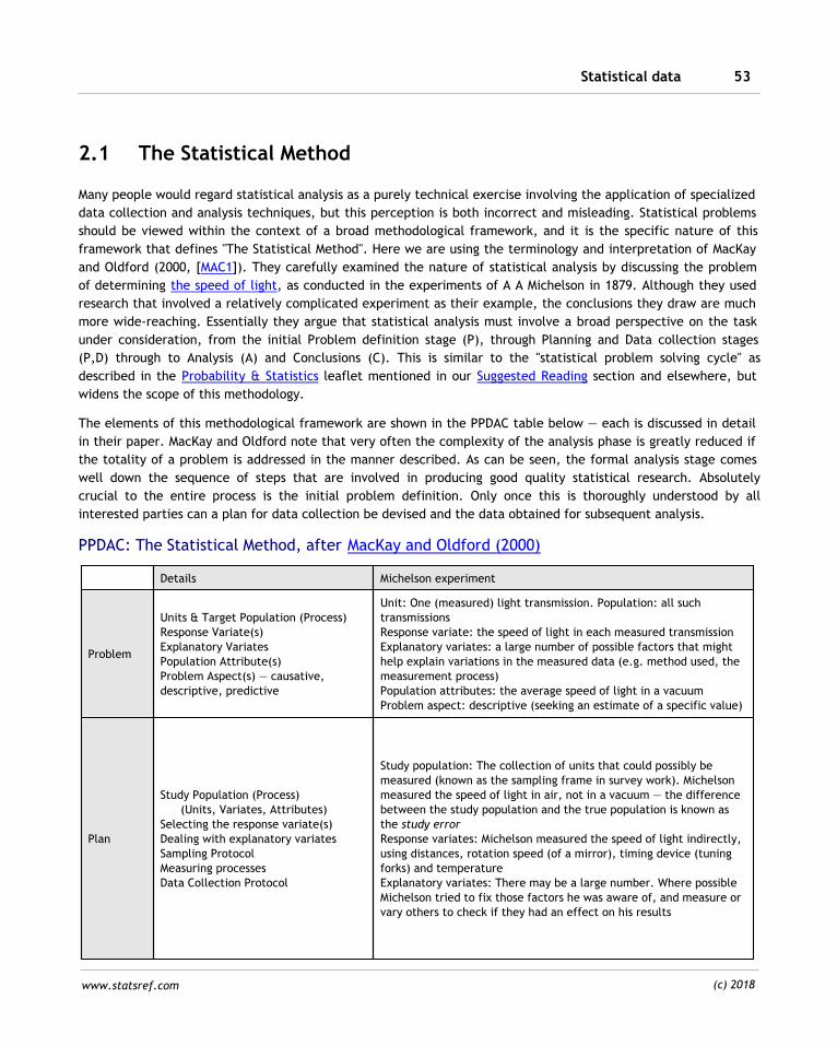
Statistical data 53

www.statsref.com (c) 2018

2.1 The Statistical Method

Many people would regard statistical analysis as a purely technical exercise involving the application of specialized

data collection and analysis techniques, but this perception is both incorrect and misleading. Statistical problems

should be viewed within the context of a broad methodological framework, and it is the specific nature of this

framework that defines "The Statistical Method". Here we are using the terminology and interpretation of MacKay

and Oldford (2000, [MAC1]). They carefully examined the nature of statistical analysis by discussing the problem

of determining the speed of light, as conducted in the experiments of A A Michelson in 1879. Although they used

research that involved a relatively complicated experiment as their example, the conclusions they draw are much

more wide-reaching. Essentially they argue that statistical analysis must involve a broad perspective on the task

under consideration, from the initial Problem definition stage (P), through Planning and Data collection stages

(P,D) through to Analysis (A) and Conclusions (C). This is similar to the "statistical problem solving cycle" as

described in the Probability & Statistics leaflet mentioned in our Suggested Reading section and elsewhere, but

widens the scope of this methodology.

The elements of this methodological framework are shown in the PPDAC table below — each is discussed in detail

in their paper. MacKay and Oldford note that very often the complexity of the analysis phase is greatly reduced if

the totality of a problem is addressed in the manner described. As can be seen, the formal analysis stage comes

well down the sequence of steps that are involved in producing good quality statistical research. Absolutely

crucial to the entire process is the initial problem definition. Only once this is thoroughly understood by all

interested parties can a plan for data collection be devised and the data obtained for subsequent analysis.

PPDAC: The Statistical Method, after MacKay and Oldford (2000)

Details Michelson experiment

Problem

Units & Target Population (Process)

Response Variate(s)

Explanatory Variates

Population Attribute(s)

Problem Aspect(s) — causative,

descriptive, predictive

Unit: One (measured) light transmission. Population: all such

transmissions

Response variate: the speed of light in each measured transmission

Explanatory variates: a large number of possible factors that might

help explain variations in the measured data (e.g. method used, the

measurement process)

Population attributes: the average speed of light in a vacuum

Problem aspect: descriptive (seeking an estimate of a specific value)

Plan

Study Population (Process)

(Units, Variates, Attributes)

Selecting the response variate(s)

Dealing with explanatory variates

Sampling Protocol

Measuring processes

Data Collection Protocol

Study population: The collection of units that could possibly be

measured (known as the sampling frame in survey work). Michelson

measured the speed of light in air, not in a vacuum — the difference

between the study population and the true population is known as

the study error

Response variates: Michelson measured the speed of light indirectly,

using distances, rotation speed (of a mirror), timing device (tuning

forks) and temperature

Explanatory variates: There may be a large number. Where possible

Michelson tried to fix those factors he was aware of, and measure or

vary others to check if they had an effect on his results

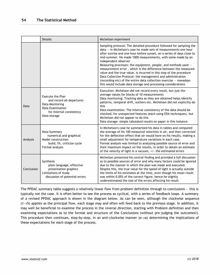
The Statistical Method54

www.statsref.com (c) 2018

Details Michelson experiment

Sampling protocol: The detailed procedure followed for sampling the

data — in Michelson's case he made sets of measurements one hour

after sunrise and one hour before sunset, on a series of days close to

mid-summer. He made 1000 measurements, with some made by an

independent observer

Measuring processes: the equipment, people, and methods used —

measurement error , which is the difference between the measured

value and the true value, is incurred in this step of the procedure

Data Collection Protocol: the management and administration

(recording etc) of the entire data collection exercise — nowadays

this would include data storage and processing considerations

Data

Execute the Plan

and record all departures

Data Monitoring

Data Examination

for internal consistency

Data storage

Execution: Michelson did not record every result, but just the

average values for blocks of 10 measurements

Data monitoring: Tracking data as they are obtained helps identify

patterns, temporal drift, outliers etc. Michelson did not explicitly do

this

Data examination: The internal consistency of the data should be

checked, for unexpected features (each using EDA techniques), but

Michelson did not appear to do this

Data storage: simple tabulated results on paper in this instance

Analysis

Data Summary

numerical and graphical

Model construction

build, fit, criticize cycle

Formal analysis

In Michelson's case he summarized his data in tables and computed

the average of his 100 measured velocities in air, and then corrected

for the deflection effect that air would have on his results, making a

small adjustment for temperature variations in each case.

Formal analysis was limited to analyzing possible source of error and

their maximum impact on the results, in order to obtain an estimate

of the velocity of light in a vacuum, +/- the estimated errors

Conclusion

Synthesis

plain language, effective

presentation graphics

Limitations of study

discussion of potential errors

Michelson presented his central finding and provided a full discussion

as to possible sources of error and why many factors could be ignored

due to the manner in which the plan was made and executed.

Despite this, the true value for the speed of light is actually outside

the limits of his estimates at the time, even though his mean result

was within 0.05% of the correct figure, hence he slightly

underestimated the size of the errors affecting his result

The PPDAC summary table suggests a relatively linear flow from problem definition through to conclusions — this is

typically not the case. It is often better to see the process as cyclical, with a series of feedback loops. A summary

of a revised PPDAC approach is shown in the diagram below. As can be seen, although the clockwise sequence

(1®5) applies as the principal flow, each stage may and often will feed back to the previous stage. In addition, it

may well be beneficial to examine the process in the reverse direction, starting with Problem definition and then

examining expectations as to the format and structure of the Conclusions (without pre-judging the outcomes!).

This procedure then continues, step-by-step, in an anti-clockwise manner (e®a) determining the implications of

these expectations for each stage of the process.

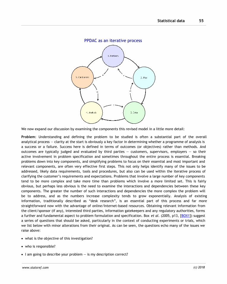
Statistical data 55

www.statsref.com (c) 2018

PPDAC as an iterative process

We now expand our discussion by examining the components this revised model in a little more detail:

Problem: Understanding and defining the problem to be studied is often a substantial part of the overall

analytical process — clarity at the start is obviously a key factor in determining whether a programme of analysis is

a success or a failure. Success here is defined in terms of outcomes (or objectives) rather than methods. And

outcomes are typically judged and evaluated by third parties — customers, supervisors, employers — so their

active involvement in problem specification and sometimes throughout the entire process is essential. Breaking

problems down into key components, and simplifying problems to focus on their essential and most important and

relevant components, are often very effective first steps. This not only helps identify many of the issues to be

addressed, likely data requirements, tools and procedures, but also can be used within the iterative process of

clarifying the customer’s requirements and expectations. Problems that involve a large number of key components

tend to be more complex and take more time than problems which involve a more limited set. This is fairly

obvious, but perhaps less obvious is the need to examine the interactions and dependencies between these key

components. The greater the number of such interactions and dependencies the more complex the problem will

be to address, and as the numbers increase complexity tends to grow exponentially. Analysis of existing

information, traditionally described as “desk research”, is an essential part of this process and far more

straightforward now with the advantage of online/Internet-based resources. Obtaining relevant information from

the client/sponsor (if any), interested third parties, information gatekeepers and any regulatory authorities, forms

a further and fundamental aspect to problem formulation and specification. Box et al. (2005, p13, [BOX1]) suggest

a series of questions that should be asked, particularly in the context of conducting experiments or trials, which

we list below with minor alterations from their original. As can be seen, the questions echo many of the issues we

raise above:

· what is the objective of this investigation?

· who is responsible?

· I am going to describe your problem — is my description correct?

The Statistical Method56

www.statsref.com (c) 2018

· do you have any past data? and if so, how were these data collected/in what order/on what days/by

whom/how?

· do you have any other data like these?

· how does the equipment work/what does it look like/can I see it?

· are there existing sampling, measurement and adjustment protocols?

Plan: Having agreed on the problem definition the next stage is to formulate an approach that has the best

possible chance of addressing the problem and achieving answers (outcomes) that meet expectations. Although

the PLAN phase is next in the sequence, the iterative nature of the PPDAC process emphasizes the need to define

and then re-visit each component. Thus whilst an outline project plan would be defined at this stage, one would

have to consider each of the subsequent stages (DATA, ANALYSIS, CONCLUSIONS) before firming up on the detail

of the plan. With projects that are more experimental in nature, drawing up the main elements of the PLAN takes

place at this stage. With projects for which pre-existing datasets and analysis tools are expected to be used, the

PLAN stage is much more an integrated part of the whole PPDAC exercise. The output of the PLAN stage is often

formulated as a detailed project plan, with allocation of tasks, resources, times, analysis of critical path(s) and

activities, and estimated costs of data, equipment, software tools, manpower, services etc. Frequently project

plans are produced with the aid of formal tools, which may be paper-based or software assisted. In many instances

this will involve determining all the major tasks or task blocks that need to be carried out, identifying the

interconnections between these building blocks (and their sequencing), and then examining how each task block is

broken down into sub-elements. This process then translates into an initial programme of work once estimated

timings and resources are included, which can then be modified and fine-tuned as an improved understanding of

the project is developed. In some instances this will be part of the Planning process itself, where a formal

functional specification and/or pilot project forms part of the overall plan. As with other parts of the PPDAC

process, the PLAN stage is not a one-shot static component, but typically includes a process of monitoring and re-

evaluation of the plan, such that issues of timeliness, budget, resourcing and quality can be monitored and

reported in a well-defined manner. The approach adopted involves consideration of many issues, including:

· the nature of the problem and project — is it purely investigative, or a formal research exercise; is it essentially

descriptive, including identification of structures and relationships, or more concerned with processes, in which

clearer understanding of causes and effects may be required, especially if predictive models are to be

developed and/or prescriptive measures are anticipated as an output?

· does it require commercial costings and/or cost-benefit analysis?

· are particular decision-support tools and procedures needed?

· what level of public involvement and public awareness is involved, if any?

· what particular operational needs and conditions are associated with the exercise?

· what time is available to conduct the research and are there any critical (final or intermediate) deadlines?

· what funds and other resources are available?

· is the project considered technically feasible, what assessable risk is there of failure and how is this affected by

problem complexity?

· what are the client (commercial, governmental, academic, personal) expectations?

Statistical data 57

www.statsref.com (c) 2018

· are there specifications, standards, quality parameters and/or procedures that must be used (for example to

comply with national guidelines)?

· how does the research relate to other studies on the same or similar problems?

· what data components are needed and how will they be obtained (existing sources, collected datasets)?

· are the data to be studied (units) to be selected from the target population, or will the sample be distinct in

some way and applied to the population subsequently (in which case, as discussed earlier, one must consider

not just sampling error but study error also)?

When deciding upon the design approach and analytical methods/tools it is often important to identify any

relevant available datasets, examine their quality, strengths and weaknesses, and carry out exploratory work on

subsets or samples in order to clarify the kind of approach that will be both practical and effective. There will

always be unknowns at this stage, but the aim should be to minimize these at the earliest opportunity, if

necessary by working through the entire process, up to and including drafting the presentation of results based on

sample, hypothetical or simulated data.

Data: In research projects that involve experiments, the data are collected within the context of well-defined and

(in general) tightly controlled circumstances, with the response and explanatory variates being clearly included in

the design of the experiment. In many other instances data is obtained from direct or indirect observation of

variates that do not form part of any controlled experiment. And in survey research, although there will be a

carefully constructed sample design, the level of direct control over variates is typically very limited. Key datasets

are also often provided by or acquired from third parties rather than being produced as part of the research.

Analysis is often of these pre-existing datasets, so understanding their quality and provenance is extremely

important. It also means that in many instances this phase of the PPDAC process involves selection of one or more

existing datasets from those available. In practice not all such datasets will have the same quality, cost, licensing

arrangements, availability, completeness, format, timeliness and detail. Compromises have to be made in most

instances, with the over-riding guideline being fitness for purpose. If the datasets available are unsuitable for

addressing the problem in a satisfactory manner, even if these are the only data that one has to work with, then

the problem should either not be tackled or must be re-specified in such a way as to ensure it is possible to

provide an acceptable process of analysis leading to worthwhile outcomes. A major issue related to data sourcing

is the question of the compatibility of different data sets: in formats and encoding; in temporal, geographic and

thematic coverage; in quality and completeness. In general datasets from different sources and/or times will not

match precisely, so resolution of mismatches can become a major task in the data phase of any project. And as

part of this process the issue of how and where to store the data arises, which again warrants early consideration,

not merely to ensure consistency and retrievability but also for convenient analysis and reporting. Almost by

definition no dataset is perfect. All may contain errors, missing values, have a finite resolution, include distortions

as a result modeling the real world with discrete mathematical forms, incorporate measurement errors and

uncertainties, and may exhibit deliberate or designed adjustment of data (e.g. for privacy reasons, as part of

aggregation procedures).

Analysis: The Analysis phase can be seen as a multi-part exercise. It commences with the review of data collected

and the manipulation of the many inputs to produce consistent and usable data. Exploratory data analysis (EDA),

including the production of simple data summaries, tabulations and graphs is typically the first stage of any such

analysis. The impact on research of exceptions — rare events, outliers, extreme values, unusual clusters — is

extremely important. Exploratory methods, such as examining individual cases and producing box-plots, help to

determine whether these observations are valid and important, or require removal from the study set. This phase

The Statistical Method58

www.statsref.com (c) 2018

then extends into more formal study in order to identify patterns of various kinds that help the researcher to

develop new ideas and hypotheses regarding form and process. And this in turn may lead on to the use or

development of one or more models within a formal build-fit-criticize cycle. Crawley (2007, p339, [CRA1])

provides the following extremely sound advice regarding model selection (echoing a quote attributed to George

Box):

"It is as well to remember the following truths about models: all models are wrong; some models are better

than others [Box said more useful]; the correct model can never be known with certainty; and the simpler a

model the better it is"!

Finally the output of the models and analysis is examined, and where necessary the dataset and data gathering

plan is re-visited, working back up the PPDAC model chain, prior to moving on to producing the output from the

project and delivering this in the Conclusion stage. The application of a single analytical technique or software

tool is often to be avoided unless one is extremely confident of the outcome, or it is the analytical technique or

approach itself that is the subject of investigation, or this approach or toolset has been specifically approved for

use in such cases. If analysis is not limited to single approaches, and a series of outputs, visualizations, techniques

and tests all suggest a similar outcome then confidence in the findings tends to be greatly increased. If such

techniques suggest different outcomes the analyst is encouraged to explain the differences, by re-examining the

design, the data and/or the analytical techniques and tools applied. Ultimately the original problem definition

may have to be reviewed.

Conclusions: The last stage of the PPDAC process is that of reaching conclusions based upon the analyses

conducted, and communicating these to others. Note that implementation of findings (e.g. actually proceeding

with building a bypass, designating an area as unfit for habitation, or implementing a vaccination programme)

does not form part of this model process, but lies beyond its confines.

“The purpose of the Conclusion stage is to report the results of the study in the language of the Problem.

Concise numerical summaries and presentation graphics [tabulations, visualizations] should be used to clarify

the discussion. Statistical jargon should be avoided. As well, the Conclusion provides an opportunity to

discuss the strengths and weaknesses of the Plan, Data and Analysis especially in regards to possible errors

that may have arisen” Mackay and Oldford (2000)

For many problems this summary is sufficient. For others the conclusions stage will be the start of additional work:

re-visiting the problem and iterating the entire process or parts of the process; a new project; implementing

proposals; and/or wider consultation. In Michelson's case, he was aware of several imperfections in his research,

and in fact spent the rest of his life conducting a series of further experiments in order to progressively improve

the accuracy of his estimate of the true speed of light. A full discussion of this revised PPDAC model in the context

of spatial analysis is provided in the "Chapter 3: Spatial analysis and the PPDAC model" of de Smith et al., 2018

[DES1] which is available online.

References

[BOX1] Box G E P,Hunter J S, Hunter W G (1978, 2005) Statistics for Experimenters: An Introduction to Design, Data Analysis and

Model Building. J Wiley & Sons, New York. J Wiley & Sons, New York. The second, extended edition was published in 2005

[CRA1] Crawley M J (2007) The R Book. J Wiley & Son, Chichester, UK, 2nd ed 2015

[DES1] de Smith M J, Goodchild M F, Longley P A and Colleagues (2018) Geospatial Analysis: A Comprehensive Guide to

Principles, Techniques and Software Tools. 6th edition, The Winchelsea Press. Available with public access from:

http://www.spatialanalysisonline.com/

Statistical data 59

www.statsref.com (c) 2018

[MAC1] MacKay R J, Oldford R W (2000) Scientific Method, Statistical Method and the Speed of Light. Statist. Sci., 15, 3, 254-

278. Available from: https://projecteuclid.org/euclid.ss/1009212817

Wikipedia, Speed of Light article: http://en.wikipedia.org/wiki/Speed_of_light

Misuse, Misinterpretation and Bias60

www.statsref.com (c) 2018

2.2 Misuse, Misinterpretation and Bias

A great deal has been written about the misuse of statistics by pressure groups and politicians, by pollsters and

advertising campaigns, by the broadcast media (newspapers, magazines, television, and now the Internet), and

even misuse by statisticians and scientists. In some instances the misuse has been simply lack of awareness of the

kinds of problems that may be encountered, in others carelessness or lack of caution and review, whilst on

occasion this misuse is deliberate. One reason for this has been the growth of so-called evidence-based policy

making — using research results to guide and justify political, economic and social decision-making. Whilst

carefully designed, peer-reviewed and repeatable research does provide a strong foundation for decision-making,

weak research or selective presentation of results can have profoundly damaging consequences. In this section we

provide guidance on the kinds of problems that may be encountered, and comment on how some of these can be

avoided or minimized. The main categories of misuse can be summarized as:

· inadequate or unrepresentative data

· misleading visualization of results

· inadequate reasoning on the basis of results

· deliberate falsification of data

In the subsections of this topic we discuss each of these categories in turn.

Where data is obtained as the result of some form of trial, experiment or survey, careful design can help avoid

many (but not all) of the problems identified in the first category (see also Design of Experiments and Bias). This

is of particular importance in medical research, and for this reason we have included a separate subsection

focusing on this particular application area and the kinds of problems and issues that are encountered.

A simple example, which occurs only too frequently, is the presentation and interpretation of data where some

data items are omitted. A much reported example of this concerned the analysis of the failure of O-rings on the

US space shuttle in 1986. NASA staff and their contractors examined the pattern of failures of O-rings during

launches against temperature just prior to the ill-fated shuttle launch on January 28 1986. They concluded that

the data showed no apparent relationship between the number of failures and temperature, but as we now know,

the low temperature overnight did result in a failure of these components (see graph below) with catastrophic

results. What the analysts failed to consider were all those launches that had 0 failures. All the launches with no

failures occurred when the ambient temperature at the launch site was much higher, as highlighted in the diagram

(see also, the Space Shuttle dataset and example in the R library, vcd).

Statistical data 61

www.statsref.com (c) 2018

In a rather different context highlighted in Jan 2010 by BBC journalist Michael Blastland (see also, our

Recommended Reading topic, [BLA1]). Reports of declining teenage pregnancy rates in Orkney off the north coast

of Scotland, were shown to be highly misleading. Blastland showed two graphs. The first appears to show a halving

of the teenage pregnancy rate between 1994 and 2006, following an intensive programme of education and

support:

However, the reports omitted data for the intervening years, and as we know from stock market and many other

types of data, rates of change depend very heavily on your start and end date. The data in this case is actually

quite cyclical, and choosing 2006 rather than, say 2007, provides a completely misleading picture, as the graph

below demonstrates.

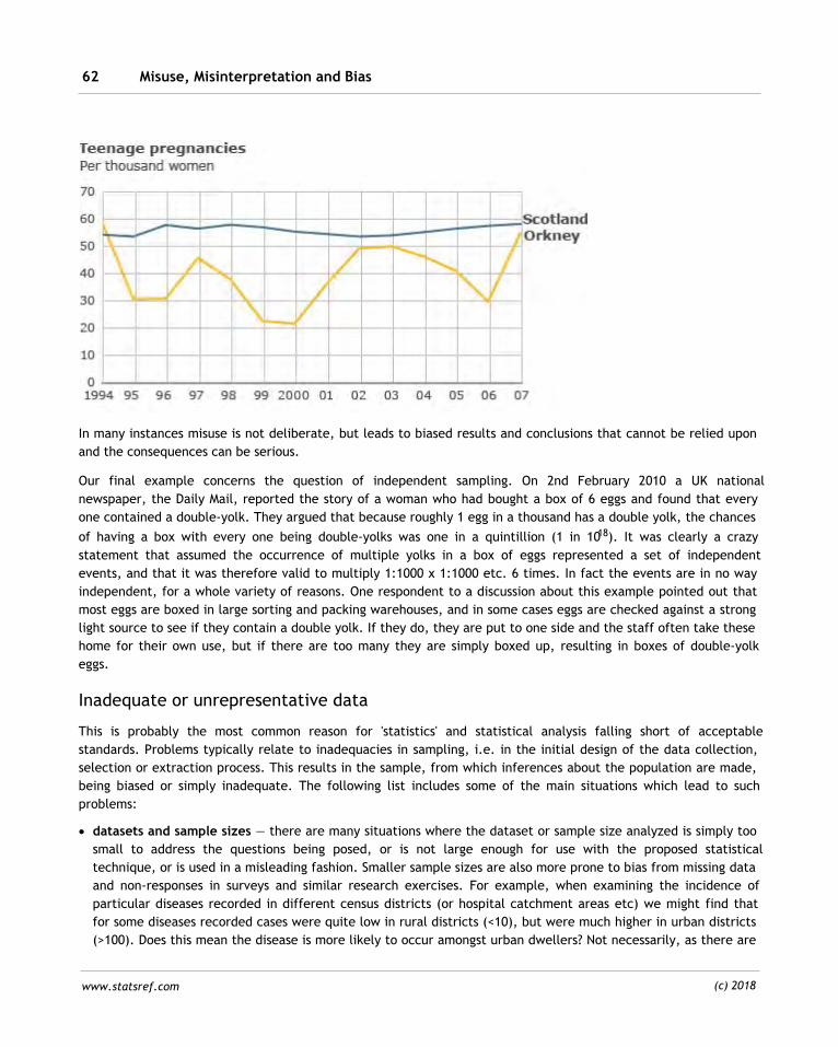
Misuse, Misinterpretation and Bias62

www.statsref.com (c) 2018

In many instances misuse is not deliberate, but leads to biased results and conclusions that cannot be relied upon

and the consequences can be serious.

Our final example concerns the question of independent sampling. On 2nd February 2010 a UK national

newspaper, the Daily Mail, reported the story of a woman who had bought a box of 6 eggs and found that every

one contained a double-yolk. They argued that because roughly 1 egg in a thousand has a double yolk, the chances

of having a box with every one being double-yolks was one in a quintillion (1 in 1018). It was clearly a crazy

statement that assumed the occurrence of multiple yolks in a box of eggs represented a set of independent

events, and that it was therefore valid to multiply 1:1000 x 1:1000 etc. 6 times. In fact the events are in no way

independent, for a whole variety of reasons. One respondent to a discussion about this example pointed out that

most eggs are boxed in large sorting and packing warehouses, and in some cases eggs are checked against a strong

light source to see if they contain a double yolk. If they do, they are put to one side and the staff often take these

home for their own use, but if there are too many they are simply boxed up, resulting in boxes of double-yolk

eggs.

Inadequate or unrepresentative data

This is probably the most common reason for 'statistics' and statistical analysis falling short of acceptable

standards. Problems typically relate to inadequacies in sampling, i.e. in the initial design of the data collection,

selection or extraction process. This results in the sample, from which inferences about the population are made,

being biased or simply inadequate. The following list includes some of the main situations which lead to such

problems:

· datasets and sample sizes — there are many situations where the dataset or sample size analyzed is simply too

small to address the questions being posed, or is not large enough for use with the proposed statistical

technique, or is used in a misleading fashion. Smaller sample sizes are also more prone to bias from missing data

and non-responses in surveys and similar research exercises. For example, when examining the incidence of

particular diseases recorded in different census districts (or hospital catchment areas etc) we might find that

for some diseases recorded cases were quite low in rural districts (<10), but were much higher in urban districts

(>100). Does this mean the disease is more likely to occur amongst urban dwellers? Not necessarily, as there are

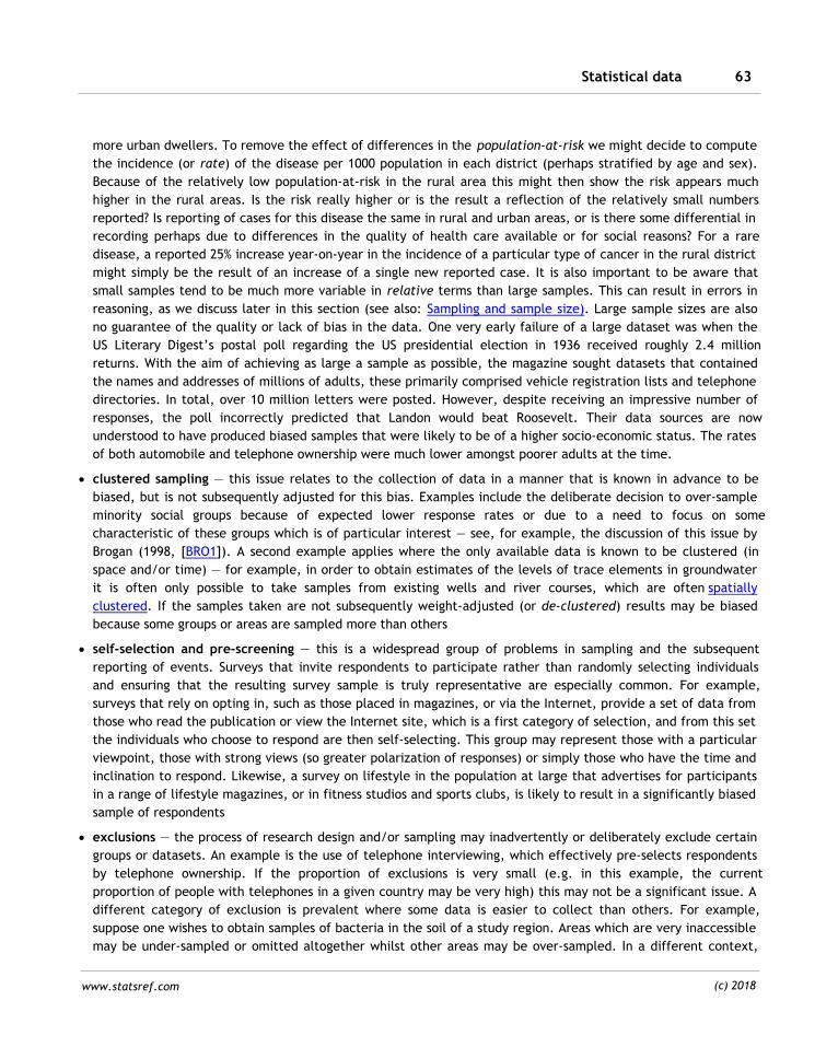
Statistical data 63

www.statsref.com (c) 2018

more urban dwellers. To remove the effect of differences in the population-at-risk we might decide to compute

the incidence (or rate) of the disease per 1000 population in each district (perhaps stratified by age and sex).

Because of the relatively low population-at-risk in the rural area this might then show the risk appears much

higher in the rural areas. Is the risk really higher or is the result a reflection of the relatively small numbers

reported? Is reporting of cases for this disease the same in rural and urban areas, or is there some differential in

recording perhaps due to differences in the quality of health care available or for social reasons? For a rare

disease, a reported 25% increase year-on-year in the incidence of a particular type of cancer in the rural district

might simply be the result of an increase of a single new reported case. It is also important to be aware that

small samples tend to be much more variable in relative terms than large samples. This can result in errors in

reasoning, as we discuss later in this section (see also: Sampling and sample size). Large sample sizes are also

no guarantee of the quality or lack of bias in the data. One very early failure of a large dataset was when the

US Literary Digest’s postal poll regarding the US presidential election in 1936 received roughly 2.4 million

returns. With the aim of achieving as large a sample as possible, the magazine sought datasets that contained

the names and addresses of millions of adults, these primarily comprised vehicle registration lists and telephone

directories. In total, over 10 million letters were posted. However, despite receiving an impressive number of

responses, the poll incorrectly predicted that Landon would beat Roosevelt. Their data sources are now

understood to have produced biased samples that were likely to be of a higher socio-economic status. The rates

of both automobile and telephone ownership were much lower amongst poorer adults at the time.

· clustered sampling — this issue relates to the collection of data in a manner that is known in advance to be

biased, but is not subsequently adjusted for this bias. Examples include the deliberate decision to over-sample

minority social groups because of expected lower response rates or due to a need to focus on some

characteristic of these groups which is of particular interest — see, for example, the discussion of this issue by

Brogan (1998, [BRO1]). A second example applies where the only available data is known to be clustered (in

space and/or time) — for example, in order to obtain estimates of the levels of trace elements in groundwater

it is often only possible to take samples from existing wells and river courses, which are often spatially

clustered. If the samples taken are not subsequently weight-adjusted (or de-clustered) results may be biased

because some groups or areas are sampled more than others

· self-selection and pre-screening — this is a widespread group of problems in sampling and the subsequent

reporting of events. Surveys that invite respondents to participate rather than randomly selecting individuals

and ensuring that the resulting survey sample is truly representative are especially common. For example,

surveys that rely on opting in, such as those placed in magazines, or via the Internet, provide a set of data from

those who read the publication or view the Internet site, which is a first category of selection, and from this set

the individuals who choose to respond are then self-selecting. This group may represent those with a particular

viewpoint, those with strong views (so greater polarization of responses) or simply those who have the time and

inclination to respond. Likewise, a survey on lifestyle in the population at large that advertises for participants

in a range of lifestyle magazines, or in fitness studios and sports clubs, is likely to result in a significantly biased

sample of respondents

· exclusions — the process of research design and/or sampling may inadvertently or deliberately exclude certain

groups or datasets. An example is the use of telephone interviewing, which effectively pre-selects respondents

by telephone ownership. If the proportion of exclusions is very small (e.g. in this example, the current

proportion of people with telephones in a given country may be very high) this may not be a significant issue. A

different category of exclusion is prevalent where some data is easier to collect than others. For example,

suppose one wishes to obtain samples of bacteria in the soil of a study region. Areas which are very inaccessible

may be under-sampled or omitted altogether whilst other areas may be over-sampled. In a different context,

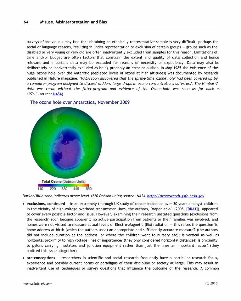
Misuse, Misinterpretation and Bias64

www.statsref.com (c) 2018

surveys of individuals may find that obtaining an ethnically representative sample is very difficult, perhaps for

social or language reasons, resulting in under-representation or exclusion of certain groups — groups such as the

disabled or very young or very old are often inadvertently excluded from samples for this reason. Limitations of

time and/or budget are often factors that constrain the extent and quality of data collection and hence

relevant and important data may be excluded for reasons of necessity or expediency. Data may also be

deliberately or inadvertently excluded as being probably an error or outlier. In May 1985 the existence of the

huge 'ozone hole' over the Antarctic (depleted levels of ozone at high altitudes) was documented by research

published in Nature magazine: "NASA soon discovered that the spring-time 'ozone hole' had been covered up by

a computer-program designed to discard sudden, large drops in ozone concentrations as 'errors'. The Nimbus-7

data was rerun without the filter-program and evidence of the Ozone-hole was seen as far back as

1976." (source: NASA)

The ozone hole over Antarctica, November 2009

Darker/Blue zone indicates ozone level <220 Dobson units; source: NASA http://ozonewatch.gsfc.nasa.gov

· exclusions, continued — in an extremely thorough UK study of cancer incidence over 30 years amongst children

in the vicinity of high-voltage overhead transmission lines, the authors, Draper et al. (2005, [DRA1]), appeared

to cover every possible factor and issue. However, examining their research unstated questions (exclusions from

the research) soon become apparent: no active participation from patients or their families was involved, and

homes were not visited to measure actual levels of Electro-Magnetic (EM) radiation — this raises the question 'is

home address at birth (which the authors used) an appropriate and sufficiently accurate measure'? (the authors

did not include duration at the address, or where the children went to nursery etc); is vertical as well as

horizontal proximity to high voltage lines of importance? (they only considered horizontal distance); is proximity

to pylons carrying insulators and junction equipment rather than just the lines an important factor? (they

omitted this issue altogether)

· pre-conceptions — researchers in scientific and social research frequently have a particular research focus,

experience and possibly current norms or paradigms of their discipline or society at large. This may result in

inadvertent use of techniques or survey questions that influence the outcome of the research. A common

Statistical data 65

www.statsref.com (c) 2018

problem is the wording of questions may lead the respondent to respond in a particular manner. Pre-

conceptions may easily also lead to weak or incorrect reasoning from the data to conclusions

· data trawling — with large multi-variate datasets there is a high probability that statistically significant findings

can be discovered somewhere in the data — brute-force processing of datasets looking for significant results

that relate to a particular area of research interest, with or without explicit pre-conceptions, will often

succeed but may well be entirely spurious. Techniques such as data-mining, cluster-hunting and factor analysis

may all be 'misused' in this way

· temporal or spatial effects — the temporal or spatial sequence or arrangement of samples may be of critical

importance, for many reasons. Examples of temporal effects include: dependence of test results on previous

tests (e.g. in wine tasting); the temporal context of research — responses to questions on a particular topic may

be very different if that topic has had a very high profile in the news in the immediate past (e.g. personal

safety, terrorism, heart disease from too much salt in the diet, attitudes to eating Beef following the BSE/vCJD

scare etc.) — this affects both the nature and the absolute levels (assigned values) of responses; temporal

effects can also be observed in data collected as a sequence using research staff whose accuracy and attention

diminish over time (for example in repeated recording of counts in microscopy; or repeated digitization of data

points, of repeated asking of questions to interviewees). Examples of spatial effects include: location

dependence (for example social groupings in specific areas, types of building, membership of organizations etc);

local correlation of results due to water, materials or other flows (e.g. contaminant levels in soil samples at

various locations may be related to each other due to groundwater or other localized effects). Missing data

(unsampled or lost data) in the temporal and spatial domains are also very common, especially with automated

monitoring equipment that may fail for brief or extended period (e.g. the NASA satellite monitoring data for

high-atmosphere ozone levels from 1978 onwards was not available for much of 1995 due to technical problems)

· over- and under-scoring — the responses individuals provide to questions or tasks often show a distinct bias.

When asked to state how confident the respondent is in the answer they have given, almost always the

confidence level is over-stated, typically by 10-20% based on the relative frequency of correct responses. In

some cultures diligence in completing surveys is taken much more seriously than in others. In one instance the

present author achieved a greater than 100% response rate to a one page questionnaire asking respondents to

list their activities on a given day — in principle impossible, but in fact many respondents photocopied the

questionnaire and completed multiple sheets, even though this was not requested. Such response patterns are

the exception — under-reporting is far more prevalent. In some instances the errors can be detected, for

example by independent measurement or using a separate survey methodology. For example, when asked to

record each telephone call made and its duration, respondents typically under-record the number of calls but

over-score the duration, often rounding up to 1- or 5-minute multiples. The product of this particular over-

scoring of duration and under-scoring of instances is generally close to the call hours (traffic, or Erlangs)

measured using automatic call monitoring equipment, so the effect in terms of traffic estimation tends to

cancel out in this case

· deliberate bias — by judicious selection, combination, arrangement and/or reporting of data (which may have

been extremely carefully collected) is an important and serious area of misuse. Examples include: deliberate

omission of data that does not fit the preconceptions of the researcher, or the conclusions they are seeking;

omission or adjustment of data (this may be acceptable practice in some instances, but should always be made

explicit — for example, exclusion of outliers on the grounds that they appear to be recording errors). Examples

in the temporal domain include reporting results for selected time periods, or against selected 'base years' to

suggest large changes that may not be of any significance; examples in the spatial domain include re-arranging

the set of zones for which reporting is being carried out to increase or decrease a particular level of a variable

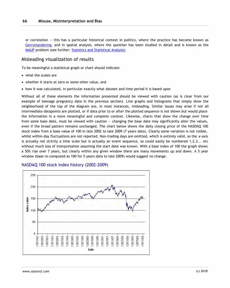
Misuse, Misinterpretation and Bias66

www.statsref.com (c) 2018

or correlation — this has a particular historical context in politics, where the practice has become known as

Gerrymandering, and in spatial analysis, where the question has been studied in detail and is known as the

MAUP problem (see further: Statistics and Statistical Analysis)

Misleading visualization of results

To be meaningful a statistical graph or chart should indicate:

· what the scales are

· whether it starts at zero or some other value, and

· how it was calculated, in particular exactly what dataset and time period it is based upon

Without all of these elements the information presented should be viewed with caution (as is clear from our

example of teenage pregnancy data in the previous section). Line graphs and histograms that simply show the

neighborhood of the top of the diagram are, in most instances, misleading. Similar issues may arise if not all

intermediate datapoints are plotted, or if data prior to or after the plotted sequence is not shown but would place

the information in a more meaningful and complete context. Likewise, charts that show the change over time

from some base date, must be viewed with caution — changing the base date may significantly alter the values,

even if the broad pattern remains unchanged. The chart below shows the daily closing price of the NASDAQ 100

stock index from a base value of 100 in late 2002 to late 2009 (7 years data). Clearly some variation is not visible,

whilst within-day fluctuations are not reported. Non-trading days are omitted, which is entirely valid, so the x-axis

is actually not strictly a time scale but is actually an event sequence, so could easily be numbered 1,2,3... etc

without much loss of interpretation assuming the start date was known. With a base index of 100 the graph shows

a 50% rise over 7 years, but clearly within any given window there are many movements up and down. A 5 year

window (base re-computed as 100 for 5 years data to late 2009) would suggest no change.

NASDAQ 100 stock index history (2002-2009)

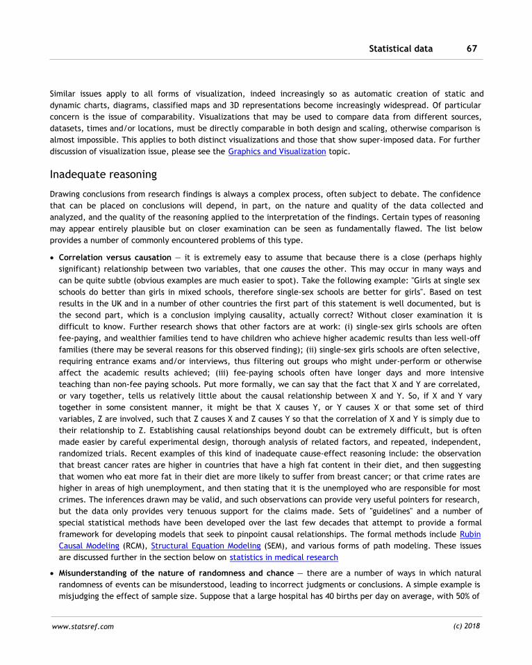
Statistical data 67

www.statsref.com (c) 2018

Similar issues apply to all forms of visualization, indeed increasingly so as automatic creation of static and

dynamic charts, diagrams, classified maps and 3D representations become increasingly widespread. Of particular

concern is the issue of comparability. Visualizations that may be used to compare data from different sources,

datasets, times and/or locations, must be directly comparable in both design and scaling, otherwise comparison is

almost impossible. This applies to both distinct visualizations and those that show super-imposed data. For further

discussion of visualization issue, please see the Graphics and Visualization topic.

Inadequate reasoning

Drawing conclusions from research findings is always a complex process, often subject to debate. The confidence

that can be placed on conclusions will depend, in part, on the nature and quality of the data collected and

analyzed, and the quality of the reasoning applied to the interpretation of the findings. Certain types of reasoning

may appear entirely plausible but on closer examination can be seen as fundamentally flawed. The list below

provides a number of commonly encountered problems of this type.

· Correlation versus causation — it is extremely easy to assume that because there is a close (perhaps highly

significant) relationship between two variables, that one causes the other. This may occur in many ways and

can be quite subtle (obvious examples are much easier to spot). Take the following example: "Girls at single sex

schools do better than girls in mixed schools, therefore single-sex schools are better for girls". Based on test

results in the UK and in a number of other countries the first part of this statement is well documented, but is

the second part, which is a conclusion implying causality, actually correct? Without closer examination it is

difficult to know. Further research shows that other factors are at work: (i) single-sex girls schools are often

fee-paying, and wealthier families tend to have children who achieve higher academic results than less well-off

families (there may be several reasons for this observed finding); (ii) single-sex girls schools are often selective,

requiring entrance exams and/or interviews, thus filtering out groups who might under-perform or otherwise

affect the academic results achieved; (iii) fee-paying schools often have longer days and more intensive

teaching than non-fee paying schools. Put more formally, we can say that the fact that X and Y are correlated,

or vary together, tells us relatively little about the causal relationship between X and Y. So, if X and Y vary

together in some consistent manner, it might be that X causes Y, or Y causes X or that some set of third

variables, Z are involved, such that Z causes X and Z causes Y so that the correlation of X and Y is simply due to

their relationship to Z. Establishing causal relationships beyond doubt can be extremely difficult, but is often

made easier by careful experimental design, thorough analysis of related factors, and repeated, independent,

randomized trials. Recent examples of this kind of inadequate cause-effect reasoning include: the observation

that breast cancer rates are higher in countries that have a high fat content in their diet, and then suggesting

that women who eat more fat in their diet are more likely to suffer from breast cancer; or that crime rates are

higher in areas of high unemployment, and then stating that it is the unemployed who are responsible for most

crimes. The inferences drawn may be valid, and such observations can provide very useful pointers for research,

but the data only provides very tenuous support for the claims made. Sets of "guidelines" and a number of

special statistical methods have been developed over the last few decades that attempt to provide a formal

framework for developing models that seek to pinpoint causal relationships. The formal methods include Rubin

Causal Modeling (RCM), Structural Equation Modeling (SEM), and various forms of path modeling. These issues

are discussed further in the section below on statistics in medical research

· Misunderstanding of the nature of randomness and chance — there are a number of ways in which natural

randomness of events can be misunderstood, leading to incorrect judgments or conclusions. A simple example is

misjudging the effect of sample size. Suppose that a large hospital has 40 births per day on average, with 50% of

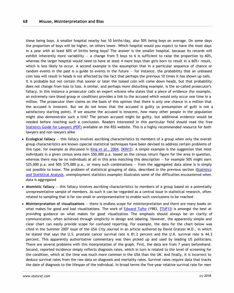
Misuse, Misinterpretation and Bias68

www.statsref.com (c) 2018

these being boys. A smaller hospital nearby has 10 births/day, also 50% being boys on average. On some days

the proportion of boys will be higher, on others lower. Which hospital would you expect to have the most days

in a year with at least 60% of births being boys? The answer is the smaller hospital, because its records will

exhibit inherently more variability — a change from 5 boys to 6 is sufficient to raise the proportion to 60%,

whereas the larger hospital would need to have at least 4 more boys than girls born to result in a 60%+ result,

which is less likely to occur. A second example is the assumption that in a particular sequence of chance or

random events in the past is a guide to events in the future — for instance, the probability that an unbiased

coin toss will result in heads is not affected by the fact that perhaps the previous 10 times it has shown up tails.

It is probable but not certain that sooner or later the tossed coin will come down heads, but that probability

does not change from toss to toss. A similar, and perhaps more disturbing example, is the so-called prosecutor's

fallacy. In this instance a prosecutor calls an expert witness who states that a piece of evidence (for example,

an extremely rare blood group or condition) provides a link to the accused which would only occur one time in a

million. The prosecutor then claims on the basis of this opinion that there is only one chance in a million that

the accused is innocent. But we do not know that the accused is guilty (a presumption of guilt is not a

satisfactory starting point). If we assume the accused is innocent, how many other people in the population

might also demonstrate such a link? The person accused might be guilty, but additional evidence would be

needed before reaching such a conclusion. Readers interested in this particular field should read the free

Statistics Guide for Lawyers (PDF) available on the RSS website. This is a highly recommended resource for both

lawyers and non-lawyers alike

· Ecological fallacy — this fallacy involves ascribing characteristics to members of a group when only the overall

group characteristics are known (special statistical techniques have been devised to address certain problems of

this type, for example as discussed in King et al., 2004, [KIN1]). A simple example is the suggestion that most

individuals in a given census area earn $50,000 p.a. based on the census return figure for the area in question,

whereas there may be no individuals at all in this area matching this description — for example 50% might earn

$25,000 p.a. and 50% $75,000 p.a., or many such combinations — from the aggregated data alone is is simply

not possible to know. The problem of statistical grouping of data, described in the previous section (Statistics

and Statistical Analysis, unemployment statistics example) illustrates some of the difficulties encountered when

data is aggregated

· Atomistic fallacy — this fallacy involves ascribing characteristics to members of a group based on a potentially

unrepresentative sample of members. As such it can be regarded as a central issue in statistical research, often

related to sampling that is far too small or unrepresentative to enable such conclusions to be reached

· Misinterpretation of visualizations — there is endless scope for misinterpretation and there are many books on

what makes for good and bad visualizations. The work of Edward Tufte (1983, [TUF1]) is amongst the best at

providing guidance on what makes for good visualization. The emphasis should always be on clarity of

communication, often achieved through simplicity in design and labeling. However, the apparently simple and

clear chart can easily provide scope for confused reporting. For example, the data for the chart below was

cited in the Summer 2007 issue of the USA City Journal in an article authored by David Gratzer M.D., in which

he stated that says the U.S. prostate cancer survival rate is 81.2 percent and the U.K. survival rate is 44.3

percent. This apparently authoritative commentary was then picked up and used by leading US politicians.

There are several problems with this interpretation of the graph. First, the data are from 7 years beforehand.

Second, reported incidence simply reflects diagnosis rates, which in turn is related to the level of screening for

the condition, which at the time was much more common in the USA than the UK. And finally, it is incorrect to

deduce survival rates from the raw data on diagnosis and mortality rates. Survival rates require data that tracks

the date of diagnosis to the lifespan of the individual. In broad terms the five-year relative survival rate for men

Statistical data 69

www.statsref.com (c) 2018

diagnosed in England in 2000-2001 was 71%. More details on survival rates for Prostate cancer over 1, 5 and 10

years can be found at the Cancer Research UK website

Prostate cancer incidence and mortality per 100,000 males per year

31 28 28 28 27 27 27

7963

49 55

110

136

104

0

20

40

60

80

100

120

140

160

180

New

Zealand

1996

Australia

1998

Germany

1997

UK 1997 France

1996

Canada

1997

USA 1997

per

100,0

00 m

ale

s

Mortality Incidence reported

.

source: Anderson and Hussey (2000, [AND1])

Deliberate falsification of data

There are occasions when data is deliberately falsified. This maybe as a result of a rogue individual scientist or

group, commercial enterprise and even government agency. The case of Prof Hwang Woo Suk who published

fraudulent results on human cloning from stem cells in 2006 is one of the most famous (see

https://en.wikipedia.org/wiki/Hwang_Woo-suk), but there is little doubt that deliberate or semi-deliberate

falsification of data is more common than many realize. Deliberate omission of results that show no significant

results or results that do not support a particular hypothesis can be regarded as a form of deliberate falsification

and is a well-established problem in academic and medical research. Recent high-profile "fake news" cases

highlight how modern media and lack of independent scrutiny can result in such issues becoming widely

circulated.

Misuse, Misinterpretation and Bias70

www.statsref.com (c) 2018

References

[ALT1] Altman D G, Bland J M (1991) Improving Doctors' Understanding of Statistics. J. Royal Statistical Society, Series A,154(2),

223-267

[AND1] Anderson G F, Hussey P S (2000) Multinational Comparison of Health Systems Data, 2000. Johns Hopkins University/The

Commonwealth Fund, October 2000. Available from: http://www.commonwealthfund.org/

[BRA1] Bradford Hill A (1937) Principles of Medical Statistics. The Lancet, London (issued in various editions until 1971. Then

republished as "A Short Textbook of Medical Statistics" in 1977

[BRA2] Bradford Hill A (1965) The Environment and Disease: Association or Causation? Proc. of the Royal Soc. of Medicine, 58,

295-300. A copy of this article is reproduced on Tufte's website: http://www.edwardtufte.com/tufte/hill

[BLA1] Blastland M, Dilnot A (2008) The Tiger That Isn't. Profile Books, London

[BRO1] Brogan D J (1998) Pitfalls of Using Standard Statistical Software Packages for Sample Survey Data. Encyclopedia of

Biostatistics. J Wiley, New York

[DRA1] Draper G, Vincent T, Kroll M E, Swanson J (2005) Childhood cancer in relation to distance from high voltage power lines

in England and Wales: a case-control study. British Medical J., 330, 4 June 2005, 1-5

[ERC1] Ercan I, Yazici B, Yang Y, Özkaya1 G, Cangur S, Ediz B, Kan I(2007) Misuage of Statistics in Medical Research. European J

General Medicine , 4(3),128-134

[HUF1] Huff D (1954) How to Lie with Statistics. W W Norton, New York

[KIN1] King G, Rosen O, Tanner M A (2004) Ecological inference: New methodological strategies. Cambridge University Press,

Cambridge UK

[TUF1] Tufte E (1983) The Visual Display of Quantitative Information. Graphics Press, Cheshire, CT.(2nd edition, 2001). Also, a

2nd, revised edition is available from Tufte's website: http://www.edwardtufte.com/tufte/books_vdqi

NASA Ozone watch information: http://ozonewatch.gsfc.nasa.gov

NADAQ 100-Index reference data: http://dynamic.nasdaq.com/dynamic/nasdaq100_activity.stm

Statistical data 71

www.statsref.com (c) 2018

2.3 Sampling and sample size

Sampling is central to the discipline of statistics. Typically samples are made in order to obtain a picture of the

population as a whole without the need to make observations on every member of that population. This saves

time, cost and may be the only feasible approach, perhaps because the population is infinite or very large or is

dynamic so sampling provides a snapshot at a particular moment. Ideally we wish to make a sample that provides

an extremely good representation of the population under study, whilst at the same time involving as few

observations as possible. These two objectives are clearly related, since a perfect representation is only possible

if the entire population is measured or if the population is completely uniform. This latter point highlights the fact

that larger and more carefully structured samples may be required to obtain an estimate of a given quality if the

population is highly variable. The difference between the measured value for an attribute in a sample from the

'true value' in the population is termed sampling error.

Typically a set of n independent samples are taken based on some form of random selection from the target

population, as far as it is possible to define the latter. Randomness in the selection process seeks to help

eliminate bias, whilst independence of samples also helps to ensure that bias due to samples being associated with

each other in some way is minimized. For example, a sample of leaves from banana trees would seek to take one

sample from each of a large number of banana trees that were relatively well separated spatially. It would be

inappropriate to take 10 different samples from one tree (the samples would not be independent as they all came

from the same tree) and likewise, trees in close proximity may exhibit similarities due to localized effects (e.g.

soil, cultivation practice, disease spread etc.) which may result in samples not being independent. Similar

considerations apply to samples taken from animals or humans, or from soils and rocks, and in some instances,

samples take over a period of time where time dependencies exist. In cases where space- and/or time-

dependencies are thought to exist, tests for autocorrelation should be carried out and if necessary, sample design

and modeling must explicitly take account of the lack of independence between observations. The procedure

adopted for any particular sampling exercise is known as the sampling protocol, and should always be carefully

planned and designed.

Target Population

The first step in this process is to define the population of interest, from which samples are to be taken. The

population may be finite or infinite, and may be very clearly defined (even if difficult to enumerate) — for

example, "all adults over the age of 18 living in a given city", or may be less well defined — for example

"particulates in the air over London", or "all measurements of outcomes from a particular industrial process".

Ensuring the nature of the population to be studied is well understood is an important step in the initial design of

any sampling scheme.

Study population

The study population is the collection of units that could possibly be measured (known as the sampling frame in

survey work). In some instances samples are made on a population that can conveniently be studied (for example,

sampling in a laboratory or a particular location) rather than sampling the population itself, with the results being

applied to the real population of interest. This results in so-called study error, which again one seeks to minimize.

In the example cited in The Statistical Method section, Michelson measured the speed of light in air on the Earth's

surface, not the speed of light in a vacuum, so the study error in this case consisted of the difference between

Sampling and sample size72

www.statsref.com (c) 2018

these two environments. In many studies the research is carried out at a particular time and location, and the

possible effects of temporal and spatial variation are excluded or deemed to have no substantive bearing on the

results. However, all research does take place in space and time, so there is always some study error related to

these factors. For example, after Michelson had completed his research, one criticism of it was that it was carried

out during a brief period of the year, which did not allow for the possibility that the findings would have been

different had the research been conducted 3 or 6 months later (reflecting the different position of the Earth

relative to the Sun). It is often helpful to ensure that the study population is as tightly defined as possible,

thereby ensuring that sampling is only from those individuals or objects that are of direct interest and helping to

restrict variation in measured attributes.

Sampling protocol

This is the detailed procedure followed for sampling the data from the study population. In many instances the

sampling protocol makes use of some level of randomization in order to avoid the risk of bias. The time, location

and possible selection from subgroups of the study population form key elements of the sampling protocol.

Controlled experiments typically involve use of a formal design that seeks to separate explanatory variables into

distinct groups, which are then systematically or randomly sampled. In many instances random numbers are

required in order to select entities, locations or times to be sampled, and typically these are computer-generated

from a uniform distribution over the range [0,1]. Random numbers may also be drawn from other distributions,

either using built-in software functions (e.g. the Excel Data Analysis tools Random Number generator facility, or

SPSS functions of the form RV.DIST which returns a random value from a distribution DIST with specified

parameters), or by using Uniform random numbers in conjunction with the cumulative distribution of interest.

In many instances a sample is required from an empirical distribution or a known (theoretical) distribution with

pre-defined parameters. Typically this involves taking a random sample from the distribution selected or from a

subset (e.g. a range) within this distribution. Many software packages provide facilities for generating such

random samples, which may then be used to compare with observed datasets or as a frame for sampling (see

further, Sampling from a known distribution).

When a large number of records have been obtained and stored in a database, samples from the dataset may be

extracted for analysis rather than analyzing the full dataset (which might consist of thousands or millions of

records). Typically samples of a pre-specified size are selected at random from the stored recordset, with checks

made to ensure that key parameters do not vary too greatly from the population values (i.e. the sample is

representative, not biased). Samples may be taken with or without replacement (without replacement is the

norm) and may be stratified if necessary, depending on the manner in which the data is stored and grouped. Most

statistical software packages provide a range of procedures for record selection. These vary from systematic to

simple random, stratified random where selection probabilities are proportional to stratum size (PPS) and many

variants on these. The table below lists the options provided for SPSS — other packages provide similar facilities.

The documentation for SPSS, SAS/STAT and other packages provide exact details of how the variants (e.g. PPS

Brewer vs PPS Murthy) are calculated. It is important to note that most standard statistical formulas assume that

records are drawn from an infinite population by simple random sampling without replacement (WOR). If this is

not the case the analytical tools applied must be adjusted to take the data selection procedure adopted into

account. Again, statistical software that facilitates such non-random selection will also include facilities for

computing core statistical measures and simple models adjusted for the sampling approach adopted.

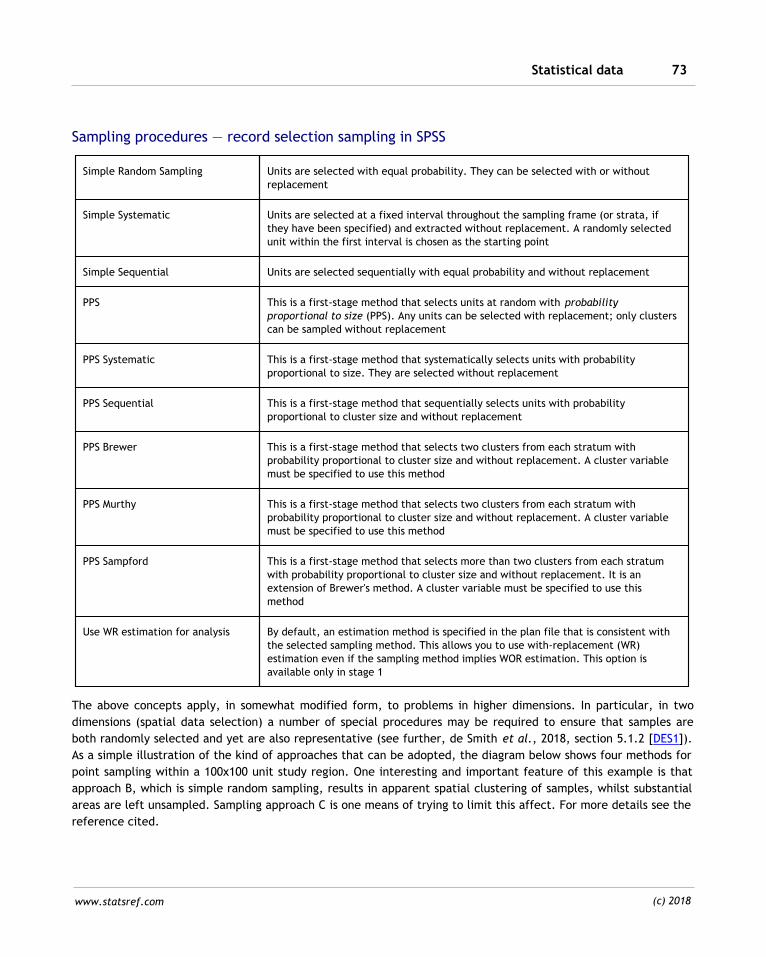
Statistical data 73

www.statsref.com (c) 2018

Sampling procedures — record selection sampling in SPSS

Simple Random Sampling Units are selected with equal probability. They can be selected with or without

replacement

Simple Systematic Units are selected at a fixed interval throughout the sampling frame (or strata, if

they have been specified) and extracted without replacement. A randomly selected

unit within the first interval is chosen as the starting point

Simple Sequential Units are selected sequentially with equal probability and without replacement

PPS This is a first-stage method that selects units at random with probability

proportional to size (PPS). Any units can be selected with replacement; only clusters

can be sampled without replacement

PPS Systematic This is a first-stage method that systematically selects units with probability

proportional to size. They are selected without replacement

PPS Sequential This is a first-stage method that sequentially selects units with probability

proportional to cluster size and without replacement

PPS Brewer This is a first-stage method that selects two clusters from each stratum with

probability proportional to cluster size and without replacement. A cluster variable

must be specified to use this method

PPS Murthy This is a first-stage method that selects two clusters from each stratum with

probability proportional to cluster size and without replacement. A cluster variable

must be specified to use this method

PPS Sampford This is a first-stage method that selects more than two clusters from each stratum

with probability proportional to cluster size and without replacement. It is an

extension of Brewer's method. A cluster variable must be specified to use this

method

Use WR estimation for analysis By default, an estimation method is specified in the plan file that is consistent with

the selected sampling method. This allows you to use with-replacement (WR)

estimation even if the sampling method implies WOR estimation. This option is

available only in stage 1

The above concepts apply, in somewhat modified form, to problems in higher dimensions. In particular, in two

dimensions (spatial data selection) a number of special procedures may be required to ensure that samples are

both randomly selected and yet are also representative (see further, de Smith et al., 2018, section 5.1.2 [DES1]).

As a simple illustration of the kind of approaches that can be adopted, the diagram below shows four methods for

point sampling within a 100x100 unit study region. One interesting and important feature of this example is that

approach B, which is simple random sampling, results in apparent spatial clustering of samples, whilst substantial

areas are left unsampled. Sampling approach C is one means of trying to limit this affect. For more details see the

reference cited.

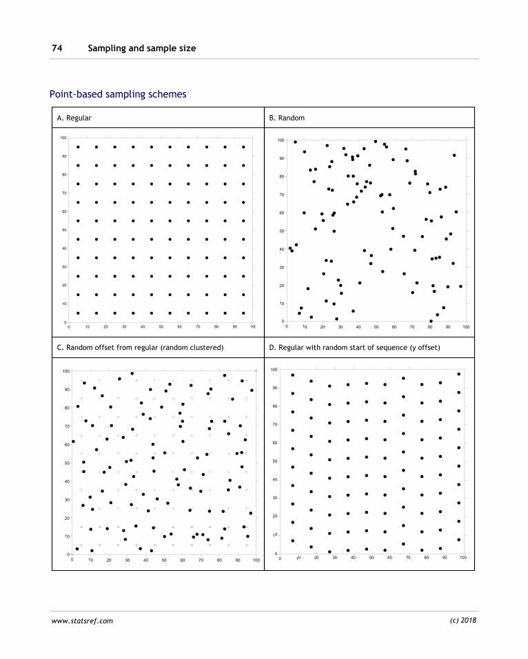
Sampling and sample size74

www.statsref.com (c) 2018

Point-based sampling schemes

A. Regular B. Random

0 10 20 30 40 50 60 70 80 90 1000

10

20

30

40

50

60

70

80

90

100

0 10 20 30 40 50 60 70 80 90 100

0

10

20

30

40

50

60

70

80

90

100

C. Random offset from regular (random clustered) D. Regular with random start of sequence (y offset)

0 10 20 30 40 50 60 70 80 90 100

0

10

20

30

40

50

60

70

80

90

100

0 10 20 30 40 50 60 70 80 90 1000

10

20

30

40

50

60

70

80

90

100

Statistical data 75

www.statsref.com (c) 2018

Sample size

There are many factors that affect the choice of sample size. In public opinion surveys it is very common to hear

that the sample taken was of around 1000-1500 people. This figure is obtained from a relatively simplistic

calculation, based on achieving an approximately 95% confidence level in the results with estimation of a

proportion, p, within a range of roughly +/-3% (see also, our discussion on confidence intervals). The figure of

1000-1500 arises from these two requirements — using a Binomial distribution the standard error (SE) of the

proportion, p, is Ö(pq/n). Note that the term Ö(pq) is maximized for any given n when p=q=0.5, so this assumption

provides an upper bound of 1/2 on Ö(pq) and thereby on the range of expected variation in our estimate. Now

from the Normal distribution, which is the limit of the Binomial for large n (and a reasonably rapid approximation

if p and q are similar in size), we know that 95% of the distribution is included within roughly +/- 2 standard

deviations. Thus the sample size needed to ensure an error in an estimate of x=5% is obtained from the formula

for 2SEs, i.e. 1/Ön. This gives the result n=1/x2 so for x=5%, x=0.05 we have n=400, or for 3% we have just over

1100. For a 1% range at 95%+ confidence a sample size of 10,000 would be required, so the choice of 1000-1500 is

a compromise between the quality of estimation and the cost and time involved in undertaking the survey.

For some problems wider bands are acceptable on the estimated proportion or mean, thus for a value within +/-

20% a sample of only 25 is required — if this was an estimate of the concentration of zinc in the soil in parts per

million (ppm), an estimate of 100ppm with a range of 80-120ppm may be perfectly acceptable. This method of

computing sample size is, of course, simply a rule of thumb that has been found to work in many situations of this

particular type. Put more formally, we are estimating the probability, a, that the estimated proportion will not

differ from the population proportion, p, by more than some amount x:

ˆPr | |p p x

If we denote by za the Normal distribution probability value for a confidence interval determined by a (e.g. with

a=0.025, two-tailed test, 5% in total, za=1.96) then this (rather simplified) formula for sample size n becomes:

2 2n z pq x

Sample size selection is thus related to several factors, including: (i) cost, time and risk; (ii) the type of problem

being addressed (and the techniques used to address the problem); and (iii) the variability of the data being

sampled. If one has prior knowledge of the data variability, or can make an informed estimate of this (for example

based on prior research and/or test samples), then the determination of sample size becomes more

straightforward. Clearly greater variability in the data will mean that the standard error (SE) is intrinsically larger,

which in turn requires a bigger sample size for a given level of precision in the parameter(s) to be estimated.

Furthermore, if the population is known to vary in some kind of structured (or stratified) manner, for example

spatially or temporally, then it makes sense to sample less frequently in the less variable phases or zones and

more frequently in those strata of the study population that are more variable. Thus a given overall sample size,

n, might represent the sum of a set of stratified samples {ni}, where each ni is separately determined from the

estimated variance, si, in zone or time slot i. There is an optimal method of determining the component samples

given n, assuming that estimates of the variance in each zone, si, are available together with some measure of the

proportions, wi, of the overall population represented by each of the separate zones or strata. With countable

items (e.g. census data) these proportions can be obtained as the count in zone i divided by the total for all

Sampling and sample size76

www.statsref.com (c) 2018

zones; other approaches might be to use areas or length of sampled time slots to determine the proportions. The

basic allocation rule is then:

1 1

, where 1

k k

i i i i i i

i i

n n w s w s w

Note that this allocation simply determines how a given sample size (perhaps obtained with reference to some

cost or time constraint) may be allocated amongst the selected strata.

Bartlett et al. (2001, [BAR1]) provide a general discussion of sample size determination for educational and social

research, drawing on the earlier work of Cochran (1977, [COC1]). Their guidance draws on the experience of many

researchers conducting questionnaire surveys and similar social research programmes. The formulas described are

based on those discussed above, but take into account issues such as: finite population size; determination of the

estimated variance; dealing with multiple measured variables of various types; and finally, dealing with non-

response. Cochran recommends, for example, that if the sample size, n, exceeds 5% of the population size, P,

then the sample size value should be adjusted by a factor n/(1+n/P). Assuming an initial sample size estimate of

400 and a population of 4000, this would adjust the sample size down to 364. If the expected response rate is 60%

the sample size is then increased to approximately 600.

A number of statistical tests, such as z-tests and t-tests, yield results that are dependent on the sample size,

through the standard error. The sections that describe these tests also provide guidance on how to compute the

sample size in order to meet requirements on the levels of Type I and Type II errors that are acceptable. Special

graphs, known as Operating Characteristic curves, provide plots of the relationship between sample size and the

two main types of error (see Ferris et. al., 1946, [FER1], for a number of such charts covering c2, F, Normal or z-

tests and t-tests).

In the medical field a range of sample size guidance documents, tables, software tools and formulas are available,

many of which are effectively variants on the same general model (see Altman [ALT1], Chow, Shao and Wang

[CHO1], Jones et al [JON1], Carley et al.[CAR1], Dupont and Plummer [DUP1], Whitley and Ball [WHI1], and

Machin et al.[MAC1]). Typically sample size estimation in these publications is based on the relationship between

three elements, two involving risk assessments and one involving the size of the effect one is seeking to discover

(small effects require larger samples in order to detect them reliably): (a) the risk of a false positive (a level,

usually taken as 5% or 0.05); (b) the risk of a false negative (b level, usually taken as 20% or 0.20; or using the

notion of power=1-b, so 80%); and (c) the size of the effect. The last item can be difficult to determine, but is

typically of the form: E=(target difference)/(estimated standard deviation). For example, if a study is trying to

detect a difference of size 14 units between a measurement on two equal sized groups (e.g. the blood pressure in

mmHg treated using different therapies, with measurements taken 6 hours after therapy commenced) and the

estimated standard deviation was 18mmHg, then the standardized effect value would be 14/18=0.78. The chart

below, redrawn from Altman [ALT1], enables the required sample size to be read from the central section by

drawing a straight line between locations on the left and right hand axes. The left hand axis shows a measure of

the size of effect one is trying to detect (in standardized units) whilst the axis on the right shows the power of the

test (as noted above power=1-the risk of a Type II error or false negative). The third element, the risk of a Type I

error or false positive is determined by the significance level in the central section.

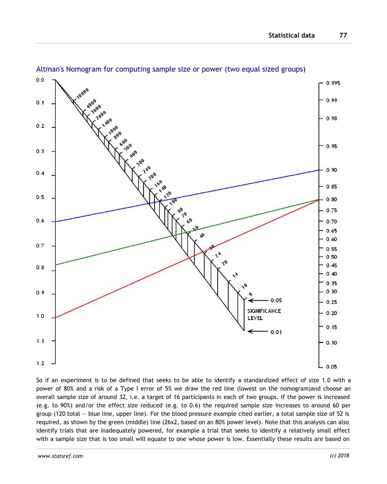
Statistical data 77

www.statsref.com (c) 2018

Altman's Nomogram for computing sample size or power (two equal sized groups)

So if an experiment is to be defined that seeks to be able to identify a standardized effect of size 1.0 with a

power of 80% and a risk of a Type I error of 5% we draw the red line (lowest on the nomogram)and choose an

overall sample size of around 32, i.e. a target of 16 participants in each of two groups. If the power is increased

(e.g. to 90%) and/or the effect size reduced (e.g. to 0.6) the required sample size increases to around 60 per

group (120 total — blue line, upper line). For the blood pressure example cited earlier, a total sample size of 52 is

required, as shown by the green (middle) line (26x2, based on an 80% power level). Note that this analysis can also

identify trials that are inadequately powered, for example a trial that seeks to identify a relatively small effect

with a sample size that is too small will equate to one whose power is low. Essentially these results are based on

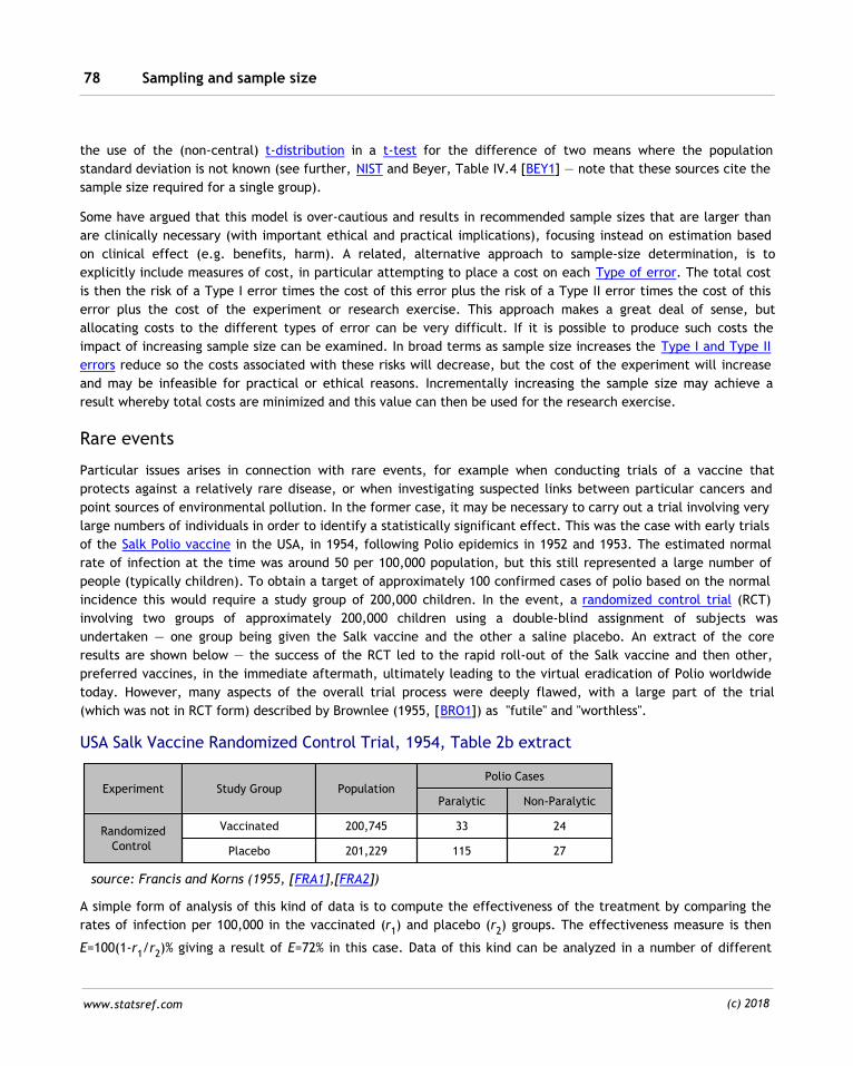
Sampling and sample size78

www.statsref.com (c) 2018

the use of the (non-central) t-distribution in a t-test for the difference of two means where the population

standard deviation is not known (see further, NIST and Beyer, Table IV.4 [BEY1] — note that these sources cite the

sample size required for a single group).

Some have argued that this model is over-cautious and results in recommended sample sizes that are larger than

are clinically necessary (with important ethical and practical implications), focusing instead on estimation based

on clinical effect (e.g. benefits, harm). A related, alternative approach to sample-size determination, is to

explicitly include measures of cost, in particular attempting to place a cost on each Type of error. The total cost

is then the risk of a Type I error times the cost of this error plus the risk of a Type II error times the cost of this

error plus the cost of the experiment or research exercise. This approach makes a great deal of sense, but

allocating costs to the different types of error can be very difficult. If it is possible to produce such costs the

impact of increasing sample size can be examined. In broad terms as sample size increases the Type I and Type II

errors reduce so the costs associated with these risks will decrease, but the cost of the experiment will increase

and may be infeasible for practical or ethical reasons. Incrementally increasing the sample size may achieve a

result whereby total costs are minimized and this value can then be used for the research exercise.

Rare events

Particular issues arises in connection with rare events, for example when conducting trials of a vaccine that

protects against a relatively rare disease, or when investigating suspected links between particular cancers and

point sources of environmental pollution. In the former case, it may be necessary to carry out a trial involving very

large numbers of individuals in order to identify a statistically significant effect. This was the case with early trials

of the Salk Polio vaccine in the USA, in 1954, following Polio epidemics in 1952 and 1953. The estimated normal

rate of infection at the time was around 50 per 100,000 population, but this still represented a large number of

people (typically children). To obtain a target of approximately 100 confirmed cases of polio based on the normal

incidence this would require a study group of 200,000 children. In the event, a randomized control trial (RCT)

involving two groups of approximately 200,000 children using a double-blind assignment of subjects was

undertaken — one group being given the Salk vaccine and the other a saline placebo. An extract of the core

results are shown below — the success of the RCT led to the rapid roll-out of the Salk vaccine and then other,

preferred vaccines, in the immediate aftermath, ultimately leading to the virtual eradication of Polio worldwide

today. However, many aspects of the overall trial process were deeply flawed, with a large part of the trial

(which was not in RCT form) described by Brownlee (1955, [BRO1]) as "futile" and "worthless".

USA Salk Vaccine Randomized Control Trial, 1954, Table 2b extract

Experiment Study Group PopulationPolio Cases

Paralytic Non-Paralytic

Randomized

Control 

Vaccinated 200,745 33 24

Placebo 201,229 115 27

source: Francis and Korns (1955, [FRA1],[FRA2])

A simple form of analysis of this kind of data is to compute the effectiveness of the treatment by comparing the

rates of infection per 100,000 in the vaccinated (r1) and placebo (r2) groups. The effectiveness measure is then

E=100(1-r1/r2)% giving a result of E=72% in this case. Data of this kind can be analyzed in a number of different

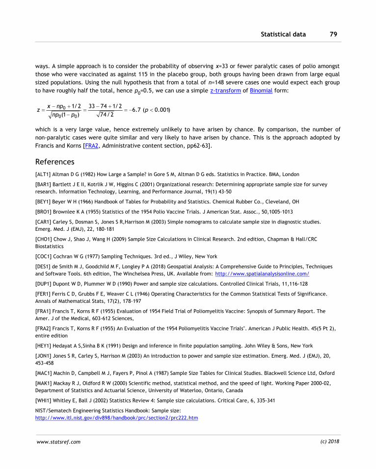
Statistical data 79

www.statsref.com (c) 2018

ways. A simple approach is to consider the probability of observing x=33 or fewer paralytic cases of polio amongst

those who were vaccinated as against 115 in the placebo group, both groups having been drawn from large equal

sized populations. Using the null hypothesis that from a total of n=148 severe cases one would expect each group

to have roughly half the total, hence p0=0.5, we can use a simple z-transform of Binomial form:

0

0 0

1/2 33 74 1/26.7 ( 0.001)

(1 ) 74/2

x npz p

np p

which is a very large value, hence extremely unlikely to have arisen by chance. By comparison, the number of

non-paralytic cases were quite similar and very likely to have arisen by chance. This is the approach adopted by

Francis and Korns [FRA2, Administrative content section, pp62-63].

References

[ALT1] Altman D G (1982) How Large a Sample? in Gore S M, Altman D G eds. Statistics in Practice. BMA, London

[BAR1] Bartlett J E II, Kotrlik J W, Higgins C (2001) Organizational research: Determining appropriate sample size for survey

research. Information Technology, Learning, and Performance Journal, 19(1) 43-50

[BEY1] Beyer W H (1966) Handbook of Tables for Probability and Statistics. Chemical Rubber Co., Cleveland, OH

[BRO1] Brownlee K A (1955) Statistics of the 1954 Polio Vaccine Trials. J American Stat. Assoc., 50,1005-1013

[CAR1] Carley S, Dosman S, Jones S R,Harrison M (2003) Simple nomograms to calculate sample size in diagnostic studies.

Emerg. Med. J (EMJ), 22, 180-181

[CHO1] Chow J, Shao J, Wang H (2009) Sample Size Calculations in Clinical Research. 2nd edition, Chapman & Hall/CRC

Biostatistics

[COC1] Cochran W G (1977) Sampling Techniques. 3rd ed., J Wiley, New York

[DES1] de Smith M J, Goodchild M F, Longley P A (2018) Geospatial Analysis: A Comprehensive Guide to Principles, Techniques

and Software Tools. 6th edition, The Winchelsea Press, UK. Available from: http://www.spatialanalysisonline.com/

[DUP1] Dupont W D, Plummer W D (1990) Power and sample size calculations. Controlled Clinical Trials, 11,116-128

[FER1] Ferris C D, Grubbs F E, Weaver C L (1946) Operating Characteristics for the Common Statistical Tests of Significance.

Annals of Mathematical Stats, 17(2), 178-197

[FRA1] Francis T, Korns R F (1955) Evaluation of 1954 Field Trial of Poliomyelitis Vaccine: Synopsis of Summary Report. The

Amer. J of the Medical, 603-612 Sciences,

[FRA2] Francis T, Korns R F (1955) An Evaluation of the 1954 Poliomyelitis Vaccine Trials". American J Public Health. 45(5 Pt 2),

entire edition

[HEY1] Hedayat A S,Sinha B K (1991) Design and inference in finite population sampling. John Wiley & Sons, New York

[JON1] Jones S R, Carley S, Harrison M (2003) An introduction to power and sample size estimation. Emerg. Med. J (EMJ), 20,

453-458

[MAC1] Machin D, Campbell M J, Fayers P, Pinol A (1987) Sample Size Tables for Clinical Studies. Blackwell Science Ltd, Oxford

[MAK1] Mackay R J, Oldford R W (2000) Scientific method, statistical method, and the speed of light. Working Paper 2000-02,

Department of Statistics and Actuarial Science, University of Waterloo, Ontario, Canada

[WHI1] Whitley E, Ball J (2002) Statistics Review 4: Sample size calculations. Critical Care, 6, 335-341

NIST/Sematech Engineering Statistics Handbook: Sample size:

http://www.itl.nist.gov/div898/handbook/prc/section2/prc222.htm

Data preparation and cleaning80

www.statsref.com (c) 2018

2.4 Data preparation and cleaning

Careful data preparation is an essential part of statistical analysis. This step assumes the data have been

collected, coded and recorded, and now reside in some form of data store. This will often be in the form of a

simple table (sometimes referred to as a data matrix) or SQL-compatible database. Depending on how the data

were coded and stored, variables may or may not have suitable descriptions, coding or data types assigned, and if

not, this is one of the first tasks to carry out. At this stage it will become apparent if any data items are

incompatible with the data type assignments, for example text coded in numeric fields, or missing data that

requires entry of a suitable 'missing data' code. Data provided from third parties, whether governmental or

commercial, should include a metadata document that describes all aspects of the data in a standardized and

thorough manner [UNI1].

Analysis of the dataset for duplicates is often the next step to undertake. There may be many reasons for

duplicates existing in datasets, these include: genuine duplicates on one or more variables; data entry errors;

multiple returns for the same case; duplicates on a subset of variables (as opposed to entirely duplicate records);

and duplicates representing deliberate coding to the same reference. Depending on the nature and validity of the

duplicates, decisions have to made on how they are to be treated. In some instances data will need to be de-

duplicated, in others data will be retained unchanged, whilst in some instances additional data will be added to

records to ensure the duplicates are separately identifiable. When analyzing duplicates using Exploratory Data

Analysis (EDA) tools, duplicates may be hidden — for example, point maps of crime incidents frequently under-

represent the concentration of crimes in certain locations as these are often recorded as co-located. Identification

of duplicates may, of itself, be a form of EDA, identifying genuine co-incident results, or perhaps highlighting data

coding protocols (such as assigning particular disease incidence to doctors surgeries or hospitals rather than the

home address of the individual).

Zero and null (missing data) occurrences form a special group of duplicates that apply to one or more variables

being studied. In many datasets the number of zeros recorded may be very large and their inclusion may totally

distort analysis of the variables in question. Software tools may provide the option to mask out (i.e. hide) zeros

from subsequent analysis. For example, a data collection device might record a value of an environmental

variable, such as wind speed and direction, every 10 minutes. For perhaps 50% of all data items logged the speed

might be below the threshold for measurement with the result that directional information also has no real

meaning. Analysis of the dataset might choose to exclude the zero values from some EDA visualizations and

statistical analyses, as these would overwhelm the results — this is not to say that such data be ignored, but that

it should be separated for some parts of the analysis.

EDA methods will also tend to highlight exceptional data values, anomalies and outliers (specific measurements or

entire cases) that require separate examination and/or removal from subsequent analysis. Note that this analysis

is taking place on the source data, not post-processed information, although the measurement and recording

process itself may have effectively pre-determined some of the possible characteristics of the source data (e.g.

the coding applied, the resolution of measurement and recording equipment, any systematic data filtering applied

during measurement or recording etc.).

In the case of outliers, there are several options of how they should be dealt with, and these will depend on the

particular problem and form of analysis being considered. If the outlier is known to be an error (e.g. a mis-coding,

by placing a decimal point in the wrong place) it can be corrected or removed. It may be an event of great

interest, in which case it warrants separate examination and analysis — this again may result in the item(s) being

Statistical data 81

www.statsref.com (c) 2018

removed from the rest of the dataset. It can also be altered in a systematic manner, for example: changing the

value to be 3 standard deviations from the mean; "Winsorizing" the value, whereby it is amended up or down to

the adjacent value in a sorted series; or effectively excluded by computing statistics based on forms of trimmed

measures, such as the trimmed mean.

Once a dataset has undergone preliminary inspection and cleaning, further amendments may be made in order to

support subsequent analyses and the use of specific statistical models. It may be desirable for such amendments

to result in the creation of a new data table or data layer, thereby ensuring that the source data remains

untouched and available for re-inspection and analysis. In some instances (very large datasets) it is preferable to

extract a representative sample of records and then apply modifications to this extracted set. Data in this new or

modified layer may be subject to re-coding, grouping into new groups or classes, and/or apply some for of data

transformation (for example applying a transformation to a continuous variable to improve the fit to the Normal

distribution). A very large number of transformations are possible, many of these being supported in standard

statistical analysis packages. For certain data types (such as temporal and spatial datasets) a specialized set of

transformations are used, which reflect the serial and neighborhood aspects of such data. For example, with

temporal data, various forms of temporal averaging, seasonal adjustments and filtering may be applied, whilst in

spatial analysis such changes may be based on local, focal or zonal computations (see further, de Smith et al.,

2018, [DES1]).

References

[DES1] de Smith M J, Goodchild M F, Longley P A (2018) Geospatial Analysis: A Comprehensive Guide to Principles, Techniques

and Software Tools. 6th edition, The Winchelsea Press, UK. Available from: https://www.spatialanalysisonline.com/

[UNI1] United Nations Statistical Commission and Economic Commission for Europe of the United Nations (UNECE) (1995)

Guidelines for the Modelling of Statistical Data and Metadata. Conference of European Statisticians, Methodological material,

United Nations, Geneva: http://www.unece.org/stats/publications/53metadaterminology.pdf)%3CBR%3E%3CBR%3EMetadata

Missing data and data errors82

www.statsref.com (c) 2018

2.5 Missing data and data errors

Missing data is a wide-ranging term for the absence of expected data from a recorded sample, which may occur

for many reasons and in many ways. In can be a small, easily managed problem, or a larger problem that raises

questions about the usability of the dataset. Missing data can involve all relevant data for a record or set of

records, or it could be missing values from a set of measurements relating to individual records (incomplete

records). Each different situation requires separate consideration, both as to the seriousness of the problem, and

to the means by which such difficulties are to be addressed. In the following paragraphs we discuss some examples

of the key issues and approaches to resolving them. We then look in more detail at some of the techniques and

tools provided within statistical software packages that are designed to assist in these situations.

In sample surveys the most common reasons are non-response, partial responses (only some questions answered)

and spoiled responses. Surveys may be structured to ensure sample sizes are increased to a level at which the

target response is achieved taking into account non-response and unusable responses, although this can be

difficult when the survey involves quotas (e.g. the study must include responses from 50 women between the ages

of 40 and 60, 50 between 60 and 80, and so forth). In general it is very difficult to avoid the problem that sample

surveys or trials will yield incomplete response data, particularly where there are many questions or variables

being examined. Such problems can lead to biased results and need to be addressed as early as possible in the

overall data collection design and implementation phase of a project. Missing data may also be encountered when

an experiment or trial is undertaken and unforeseen circumstances make some of the data unusable or impossible

to obtain. For example, the present author conducted a controlled trial of three different types of multi-lingual

keyboard in the European Commission headquarters in Brussels. A total of 96 staff were recruited (48 for week 1,

48 for week 2) to undertake computer-controlled typing tests in a variety of real and synthetic languages. All test

sessions were completed with no data losses until one morning the building was picketed and attacked by French

farmers protesting against proposed changes to the Common Agricultural Policy. They entered the building and

were only removed after tear gas was used, which in turn shut down the lower levels of the building and our

morning's data session was lost! Fortunately the exercise included enough replicates, including a complete

replicate of the entire experiment in week 2, so analysis of the results was only marginally affected (see Evans,

1988 [EVA1]). In trials of medical procedures one or more of those involved in the trial may be unable to complete

the trial due to illness or other, unrelated factors, or maybe one sample becomes contaminated or is not of the

correct strength, so the data has to be discarded. This may be all the data relating to one or more participants in

the trial, but more commonly relates to one or data items relating to a case — for example, a missing test result.

Datasets that rely on remote-sensing equipment frequently demonstrate missing data, when equipment fails or has

to be taken out of use temporarily for servicing or other reasons.

For certain experiments and analyses, such as some randomized block designs, loss of even a single data item is

important because it upsets the balanced nature of the design and its subsequent analysis. Where observations are

unavailable for a single unit this may be partially overcome by estimating or imputing the missing data from the

remaining information, thereby turning the unbalanced design back to a balanced form. For example, in a

randomized block design (see further, Cox, 1958 [COX1]) with k blocks and t treatments a simple estimate for a

single missing value is given by (kB-tT-G)/(k-1)(t-1) where B is the total of all remaining observations in the block

containing the missing observation, T is the total of observations on the missing treatment, and G is the grand

total. This provides a simple form of averaging for a single missing value — least squares techniques or simple

iterative estimation can be used to extend the concept to more than one missing value. Analysis then continues as

if the estimated value or values were genuine, but with residual degrees of freedom reduced by 1 for each missing

Statistical data 83

www.statsref.com (c) 2018

value and a correction for bias applied to the total sums of squares in the Analysis of Variance computation.

Likewise, in time series analysis, complete time series are almost always required, making analysis of incomplete

temporal datasets very problematic. Where such data is missing at the start or end of a series, it may be sufficient

to simply ignore this problem and analyze the data that is available, assuming that it can be regarded as

representative of the entire period. However, if embedded values (i.e. within the series) are missing some form of

estimation is often the only option.

Another common reason for missing data is incorrect data recording, coding or subsequent processing. The precise

reason for such errors and the scale of the problem are important to determine. Incorrect data coding by

researchers and data preparation staff can often be checked through systematic verification, for example by

taking a sample of each block of survey returns and having these independently recoded and compared with the

original coding. Incorrect interpretation of survey questions, or incorrect recording of data by surveyed

individuals, needs to be identified through inspection and validation techniques, thereby identifying the scale and

nature of any problems, and implementing changes or corrections to the data gathering and/or subsequent

processing of the data. The widely publicized issue of data quality associated with the Climate Science Unit (CSU)

at East Anglia University in the UK (see http://www.cru.uea.ac.uk/cru/data/availability/ and the IPCC dataset

site: http://www.ipcc-data.org/ ) provides a vivid insight into some of the issues associated with collating and

cleaning datasets from multiple sources on a range of variables over a prolonged period of time.

Minor errors and occasional items of missing data can often be handled programmatically, but in some cases such

approaches are not sufficient and the data and project will have to be reviewed in the light of the data

limitations. Many software packages include facilities to handle problems with data completeness. The most

common arrangement is for data to be coded to identify missing values, for example using a distinct entry such as

a blank " ", * or -999 to indicate a missing value, depending on the data type and range being recorded. When an

entry of this kind is encountered, the software package will apply one or more rules in order to determine what

action to take. For example, in computing basic statistics for quantitative datasets it may simply ignore missing

values (as opposed to deleting records with missing values) and carry out the computation on the available subset,

with a reduced count of items. This raises the question as to whether such estimates are biased.

It is not merely the scale of missing items that must be considered, but also whether there is any pattern to the

missing data. If the missing values occur completely at random (MCAR) and the proportion of missing values is not

large (<5%) then statistics such as mean values, variances, correlations etc. can be produced ignoring these

missing values and the results will tend to be unbiased. However, if the missing values are not randomly

distributed throughout the data, bias will be apparent. It is possible that the non-randomness of missing values is

partial, in the sense that within groups the missing values occur randomly but between groups there are

substantial differences. This might be observed in cases where one group in more likely to respond to a question

or to perform a task than another group. If the data show missing at random (MAR) data within groups but do not

conform to the MCAR requirement, it is still possible to produced unbiased statistics within these groups. It may

also be possible/acceptable to fill in missing values with estimated values that are derived from the remaining

data in the entire study or subsets of the study — this applies principally to quantitative data in univariate and

multivariate data sets, and to temporal and spatial datasets.

In order to determine whether MCAR, MAR or neither apply, the dataset can be partitioned and subject to various

forms of simple pattern analysis and statistical comparisons. For example, all records could be divided into those

with and without a data value on a given variable, and a comparison statistic (such as Little's chi-squared test,

[LIT1, LIT2]) computed to try and detect any significant differences between the two subsets. Having identified

Missing data and data errors84

www.statsref.com (c) 2018

the scale and nature of the missing data problem, the question then arises as to what action to take. If the sample

size is large enough and the proportion of records with missing data is small, it may be acceptable to either ignore

the missing values (especially if the MCAR or MAR tests indicate that this is very safe to do), or to delete/ignore

entire records with missing values (generally an unsafe practice, as this tends to introduce additional bias), or to

impute the missing data (see further, below) from the remaining records. In this latter case missing data are

essentially 'invented' by reference to other data in the sample. Typically results are then reported with and

without the imputed data, with a clear explanation of the impact of imputation on the results.

There are many techniques for such imputation, notably maximum likelihood and a variety of regression methods.

Pure multiple regression methods tend to underestimate the true variance of the imputed data values, so some

form of variance inflation may be added to overcome this limitation. So-called multiple imputation (MI) methods

are now favored by some researchers since these appear to provide more representative and robust results (see

further, Pickles, 2005, [PIC1]). MI methods involve some form a conditional simulation, producing several

imputations (typically 5-10) and then using the mean of the results as the estimates for the missing values.

Alternatively the entire analytical procedure can be carried out on each of the versions of the dataset, and the

results from each analysis averaged or compared. Typically such methods will compute the mean and variance of

the variable across records for which complete data is available and then sample random values from the Normal

distribution matching these parameters to obtain sample values for the missing item. Some packages, such as

SAS/STAT, perform MI using samples obtained via MCMC methods (essentially this involves using the remaining

data as a model distribution for the missing data and randomly sampling from this model distribution). For

categorical data samples are taken from a Multinomial distribution. Another approach, which is sometimes usable

with categorical data, is to create a new category that contains those records that include missing data.

Similar concepts have been applied in temporal and spatial analysis, both as a form of missing data analysis and as

a form of prediction or estimation for unsampled times and locations. For example, the use of conditional

simulation is now a preferred form of prediction in geospatial engineering applications, such as oil and mineral

prospecting. If there are very few missing data points in dense temporal or spatial datasets it is usual for these to

be estimated using deterministic procedures, using linear, bi-linear or spline interpolation from their immediate or

near-neighboring data items, or using simple mean or median values in the local neighborhood. The quality of

imputed results can be evaluated by comparison with the entire dataset (e.g. convergence of parameters), by

internal consistency checks (e.g. jackknifing and bootstrapping techniques) and/or by reference to external

datasets and samples (e.g. so-called 'ground truth' comparisons).

Handling missing values — techniques and tools

This section provides a brief summary of the main approaches for handling missing values. In most instances these

are procedures offered within software packages, but it remains the responsibility of the researcher to select the

method used and to document and justify such selection when reporting the results of analysis. In many cases

estimating missing values will apply to real-valued measurements, but some procedures may apply to binary or

categorical data.

Ignoring entire records

This is the most commonly available approach for handling missing data. As noted above, this is only acceptable if

the number records is relatively large, the number of records with missing data is relatively small (<5%), and the

missing records can be shown to occur completely at random (MCAR) or are missing at random (MAR) within well-

Statistical data 85

www.statsref.com (c) 2018

defined subsets of the data. In general this approach cannot be used in small sample balanced trials nor for time

series.

Setting missing values to fixed value

Many packages allow missing values to be replaced with a fixed value (e.g. 0) or a user-provided value for each

instance. The problems of adopting these approaches are obvious.

Single estimation procedures

A very common approach to missing values is to use some form of estimation based on the characteristics of the

data that has been successfully collected. For example, the SPSS Transform operation, Missing Values option,

offers the following options for estimating such values: (i) use of the mean or median value of nearby points (by

which it means neighboring records, with the number of such records used selectable by the researcher); (ii) use

of the overall series mean, i.e. the mean based on all records; (iii) linear interpolation, which applies to data in

series and uses the two adjacent non-missing values, to fill in the gap or gaps; (iv) linear regression, which is

similar to linear interpolation but use a larger number of neighboring points and calculates a best fit line through

these as its estimator for intermediate missing values. Other software packages may provide additional options —

for example, a variety of model-based interpolation options are available in the SAS/ETS (Economic and Time

Series) software. Similar procedures are provided in some other packages, but often it remains the researcher's

responsibility to provide or compute estimates for missing values as a part of the data cleaning and preparation

stage.

Multiple imputation (MI)

Multiple imputation (MI) methods vary depending on the type of data that is missing and the software tools used

to estimate (impute) the missing values. In this subsection we describe the approaches adopted by the SAS/STAT

and SPSS software, which are largely based on the published work of Rubin (1976, 1987, 1996 [RUB1],[RUB2],

[RUB3]).

Essentially there are 3 stages to MI:

· the missing data are filled in m times to create m complete datasets (m is typically 5)

· the m complete datasets are analyzed separately, in the usual manner

· the results from the multiple analyses are combined in order to provide statistical inferences regarding the data

Depending on the type and pattern of missing data, SAS/STAT and SPSS will generate estimates for the missing

values using some form of regression analysis of the valid data (single, multiple or logistic regression), or MCMC

methods under an assumption of multivariate Normality, for more general missing values. The latter approach is of

the general form: (a) initialize estimates for the missing values for all records and variables by drawing random

values from a Normal distribution with mean and variance that match the non-missing data (or use a multinomial

distribution for categorical data, with proportions in each class defined by the proportions in the non-missing

data); (b) using all the data, except for missing data on the jth variable, use a univariate method (e.g. regression)

to impute the missing values in that variable; (c) iterate across all variables and track the convergence of both the

mean and variance of the imputed missing values.

When the datasets are analyzed the results are combined to produce a single set of inferences together with the

between and within imputed dataset covariances. As Rubin (1996, p476, [RUB3] ) explains, the posterior

Missing data and data errors86

www.statsref.com (c) 2018

distribution of the data obtained following multiple imputations is simply the average of the individual

imputations, the mean values are the means of the imputations, and the variances are the sum of the average of

the individual variances obtained from the MI process plus the variance of the mean values obtained.

References

[COX1] Cox D R (1958) Planning of experiments. John Wiley & Sons, New York

[EVA1] Evans S (1988) The statistical aspects of a study to help in the design of a multi-lingual keyboard. MSc. thesis, University

of Kent, UK

[LIT1] Little R J A, Rubin D B (1987) Statistical analysis with missing data. John Wiley & Sons, New York

[LIT2] Little R J A (1988) A test of missing completely at random for multivariate data with missing values. J of the American

Statistical Association, 83, 1198-1202

[PIC1] Pickles A (2005) Missing data, problems and solutions. pp. 689-694 in Kempf-Leonard K, ed., Encyclopedia of social

measurement. Elsevier, Amsterdam

[RUB1] Rubin D B (1976) Inference and Missing Data, Biometrika, 63, 581-592.

[RUB2] Rubin D B (1987) Multiple Imputation for Nonresponse in Surveys. New York: John Wiley & Sons.

[RUB3] Rubin D B (1996) Multiple Imputation after 18+ Years. Journal of the American Statistical Association, 91, 473-489

Statistical data 87

www.statsref.com (c) 2018

2.6 Statistical error

When approaching any form of data analysis many types and sources of error may be considered: the data

collection procedure may contain errors; there may be gross data capture or encoding errors; there may be errors

in the approach adopted to selecting data, designs or in analysis. However, none of these relates to the rather

special use of the term statistical error. This term refers specifically to non-systematic or random errors that are

observed during measurement. There may be many reasons why such random variations occur, but in general the

assumption is made that these reasons are unknowable and therefore cannot be readily removed. Systematic

variations and gross errors can, at least in theory, be separated out and either accounted for or removed, leaving

simply statistical error.

Statistics in Medical Research88

www.statsref.com (c) 2018

2.7 Statistics in Medical Research

Statistical methods as applied to problems in medical research are, at first sight, no different from the application

of such methods to any area of scientific endeavor. However, there are some important societal and technical

aspects of medical research that warrant particular attention. At the societal level the issues relate to the impact

on individual patients of intervention procedures, treatments and their side effects. The conduct and

interpretation of medical trials is an extremely important issue, and decisions made regarding who is to be treated

and how, and who is not to be treated, are often complex and can be distressing for all involved. Furthermore,

inadequate design, implementation and reporting of trials can lead to erroneous conclusions, with potentially

serious consequences. On a technical level there are specific techniques and protocols that have been developed

to address many of these issues, but there remains continuing difficulties facing medical staff who need to

understand and use appropriate statistical procedures whilst having an enormous number of other issues to deal

with. Again, these problems can be addressed by early involvement of medical statisticians, although the scarcity

of experienced specialists in this field is an additional concern. There is also an ongoing debate regarding the

appropriateness of classical frequentist statistics, and even Bayesian statistics to many problems in medical

research, bearing in mind the practical complexities and uncertainties associated with such work, especially for

observational studies.

In 1937, the editor of The Lancet, writing in the foreword of Austin Bradford Hill's groundbreaking book "Principles

of Medical Statistics" [BH1] summarized the position of statistics in medicine at that time as follows:

"In clinical medicine today there is a growing demand for adequate proof of the efficacy of this or that form

of treatment. Often proof can come only by means of a collection of records of clinical trials devised on such

a scale and in such a form that statistically reliable conclusions can be drawn from them. However great

might be our aversion to figures, we cannot escape the conclusion that the solution of most of the problems

of clinical or preventative medicine must ultimately depend on them"

Bradford Hill sought to provide an easily understood introduction to statistical concepts and methods for medical

students, and his book [BH1] continued to be updated and published in many editions and in many translations,

over a period of forty years. He was particularly concerned to ensure that the foundations of medical research

benefited from sound underlying logical analysis and testing. To this end he was one of the initial proponents of

randomized controlled trials (RCTs), which provide a key framework for current medical research exercises. In

addition he devised a series of viewpoints on how suspected cause-effect relationships can be evaluated. Both of

these areas are discussed in more detail below.

Bradford Hill was also extremely influential in bringing the idea of cohort studies to the fore through his work with

Sir Richard Doll on the link between smoking and lung cancer. Their initial research was based on a case-control

approach, but they then extended this work to a cohort study of over 30,000 British doctors. Cohort studies

typically involve tracking the medical histories of a select group or cohort of individuals over many years. For

example, in 2010 an international cohort study known as COSMOS was launched. The UK cohort will follow the

health of approximately 100,000 mobile phone users (18+ years old) for 20-30 years, and the international cohort

will follow approximately 250,000 European mobile phone users over this period.

Considerable efforts have been made by many specialists with the aim of improving the understanding of statistics

by medical professionals and in ensuring the quality of reporting in journal publications is of the highest standard

(see especially the excellent article and associated discussion in Altman and Bland, 1991 [ALT1]). The quality of

published studies has been greatly aided by the production or adoption of guidelines by individual journals, and by

Statistical data 89

www.statsref.com (c) 2018

the development of "statements" that explain how different types of research exercise should be reported.

Perhaps the most important of these is CONSORT: "Consolidated Standards of Reporting Trials", which encompasses

various initiatives to alleviate the problems arising from inadequate reporting of randomized controlled trials

(RCTs). We discuss CONSORT further below. Other examples of such statements include STROBE "Strengthening

the Reporting of Observational studies in Epidemiology", and the EQUATOR network, which is an international

effort that seeks to "improve the reliability and value of medical research literature by promoting transparent and

accurate reporting of research studies". Their 'reporting guidelines' section includes links to many useful websites

and articles, including those already mentioned, and articles such as Olson et al. [OLS1] on the reporting of case-

control studies.

As mentioned earlier, undertaking and reporting of medical research requires many specialized skills. Historically

there has been insufficient training of medical researchers in statistical concepts and methods, and very real

problems of communication between medical and statistical specialists. For example, the terms significance,

variance and frequency may have a very different meaning to medical staff from those assigned by statisticians.

To medics significance has the more usual interpretation of 'being significant' or important in the context of the

medical problem under consideration — indeed, statisticians and medical journals now often play down the use of

the term and the associated use of statistical significance levels (p-values). Estimation (identifying the typical

range of values/effects) is rightly regarded as being of far greater relevance. For those involved in case-mix

management (CMM) analysis of variance may refer to financial management (variation from targets) rather than

having any statistical interpretation, whilst frequency can refer to how often a patient visits the toilet! As with

many disciplines, technical terminology unfortunately may serve to confuse rather than clarify the subject.

There is no simple answer to these problems, although modern undergraduate and post-graduate teaching practice

attempts to address the most important issues in a manner that medical specialists are most likely to respond to

and retain, long after the brief courses given have been completed. The leading medical journals, key medical

reference web sites, the early involvement of medical statisticians, statistical consultancy and peer review,

recently published precedents and the application of sound methodologies (such as the PPDAC model discussed

earlier in this Handbook) will all serve to assist those engaging in medical research and trials for the first time.

The technical statistical procedures applicable to medical research are covered in the various main topics and

sections of this Handbook. However, there are one or two specific topics that warrant further comment at this

juncture. The two we have focused upon are Causation, and the Conduct and Reporting of Research. Each of these

topics is discussed briefly in the subsections that follow.

An equally important topic, which is of particular relevance to medical research, is that of Bayesian analysis. We

have discussed aspects of Bayesian analysis earlier in this Handbook (e.g. see Yudowsky's example of breast cancer

screening). Whilst not excluding classical frequentist statistics, a substantial number of scientists believe that

Bayesian thinking is essential in the medical sphere — as Professor Campbell states in his commentary on Altman

and Bland's paper (see also [CAM1]):

"Many doctors have an 'a priori' belief that the patient either has or does not have the disease and use the

Bayesian paradigm to modify their beliefs. They find the idea of a null hypothesis existing without any

probability attached to it counter-intuitive"

Other authors argue that for some problems only a Bayesian approach can provide a sensible answer, or in some

instances, any answer at all.

Statistics in Medical Research90

www.statsref.com (c) 2018

We now take a closer look at the thorny question of causality, and how suspected cause-effect relationships can

be identified and studied. We then consider some aspects of the conduct and reporting of medical research,

including randomized controlled trials (RCTs), case-control studies and cohort studies. These procedures are a

particular feature of modern medical research and RCT in particular is a development that has been largely

championed in the medical statistics field.

References

[ALT1] Altman D G, Bland J M (1991) Improving Doctors' Understanding of Statistics. J of the Royal Stat. Soc., A, 154(2), 223-267

[BH1] Bradford Hill A (1937) Principles of Medical Statistics. The Lancet, London (issued in various editions until 1971. Then

republished as "A Short Textbook of Medical Statistics" in 1977

[BH2] Bradford Hill A (1965) The Environment and Disease: Association or Causation? Proc. of the Royal Soc. of Medicine, 58,

295-300. A copy of this article is reproduced on Tufte's website: http://www.edwardtufte.com/tufte/hill

[CAM1] Campbell M J, Machin D, Walters S J (2007) Medical Statistics : A Textbook for the Health Sciences. 4th Ed., John Wiley

& Sons Ltd, Chichester

[OLS1] Olson S H, Voigt L F, Begg C B, Weiss N S (2002) Reporting participation in case-control studies. Epidemiology,13(2),123-6

2.7.1 Causation

In our earlier discussion of the problems associated with using and interpreting statistical data we described some

of the difficulties involved when trying to establish and model causation. As Rothman et al. (2008, p5 [ROT1])

observe:

"such a model should address problems of multifactorial causation, confounding, interdependence of effects,

direct and indirect effects, levels of causation, and systems or webs of causation"

In medical statistics the word cause is often used in a probabilistic sense, i.e. by suggesting that factor A is a

cause of outcome or disease B, we often mean that A significantly increases the risk or probability of outcome B.

This lack of specificity reflects an underlying uncertainty about the detailed processes at work. Hence recognizing

that a particular chemical is carcinogenic does not explain the processes that lead from exposure to incidence of

the condition — these processes are likely to be extremely complicated involving molecular biology, and may be

difficult if not impossible to determine.

In a famous paper delivered by Austin Bradford Hill to the Royal Society of Medicine in 1965 [BH2], he suggested a

series of viewpoints (his terminology) by which one might use as guidance when seeking to establish the nature

and validity of a suspected causal relation. In this subsection we summarize what has now become known as the

Bradford Hill Criteria, although the term criteria was not used in his paper. He commences with the assumption

that a clear-cut association (or correlation) of some kind has been observed. This association is not assumed to be

one that has been obtained as statistically significant — in fact, Bradford Hill argues strongly against the blind use

of statistical significance in this context. In addition and as noted above, the causal relationship may in fact be

complex, as for example in a causal chain, or in an effect that may be the result of multiple (i.e. different) causal

factors or the result of several factors working in combination. Bradford Hill's nine viewpoints for examining

possible causal effects are, in summary:

Statistical data 91

www.statsref.com (c) 2018

Bradford Hill's (1965) 9 Viewpoints for Causation

1. Strength: if an association is very strong it deserves closer consideration than weaker associations — for

example, if we observe that heavy smokers are 30+ times more likely to contract lung cancer than non-

smokers, the strength of evidence is more powerful than if we observed that they were only 2x as likely to

contract lung cancer. In fact it was Bradford Hill who first brought this particular relationship to public

attention. On the other hand, lower strength of evidence does not imply that there is no causal relationship

2. Consistency: is the observed association repeated/repeatable, in different locations, at different times and

under differing circumstances? As above, the absence of such repeatability does not imply that there is no

causal relationship — for example, it may not be possible to repeat a set of circumstances

3. Specificity: if the observed association appears to be highly specific to a given set of circumstances and/or

locations, then it is more likely to be related to these circumstances in some causal manner. For example, the

very high incidence of certain diseases amongst individuals working in very specific environments (e.g.

chimney sweeps in the 18th and 19th centuries; Nickel refinery workers in the early 20th century). A

somewhat different example is the incidence of pre-menopausal breast cancers where a high number of cases

has been observed within particular families across the generations, suggesting a specific genetic effect

4. Temporality: here the question is whether the order is A®B or B¬A. For example, is being extremely

overweight causing people to contract a particular disease or condition, or do people with a particular

condition become extremely overweight. These kinds of relationships can be quite subtle and inter-connected

5. Biological gradient: if increased exposure to some well-defined hazard is associated with a similarly increase in

disease incidence, then this tends to support a causal relationship, as compared with a relationship for which

no 'gradient effect' is observed

6. Plausibility: if the suspected causal relationship is plausible, within the scope of current knowledge, then it

has (marginally) more merit than a relationship for which no known explanation can be proposed. Having made

this observation, it is clearly a relatively weak criterion

7. Coherence: if the suspected causal relationship is consistent with current knowledge about the variables

involved, it may help to support (or at least, not to detract from) the possible causal relationship being

considered. Again, as with plausibility, this may be regarded as a relatively weak criterion

8. Experiment: if one or more repeatable controlled experiments can be carried out to test the suspected

causality, and these tests support the hypothesis, this greatly enhances the strength of evidence case

9. Analogy: if a similar causal relationship has been established, but under different circumstances, it may again

provide support for the argument that a causal relationship exists, but again this is a weak criterion

These 9 viewpoints have been taught to students in the biomedical sciences for many years, often as criteria

rather than as broad guidance. More recently authors such as Phillips and Goodman [PH1] have re-emphasized the

original 'lessons' of Bradford Hill, in particular his skepticism regarding the use of statistical significance. In their

commentary they summarize these missing lessons as:

· Statistical significance should not be mistaken for evidence of a substantial association

· Association does not prove causation (other evidence must be considered)

· Precision should not be mistaken for validity (non-random errors may exist)

Statistics in Medical Research92

www.statsref.com (c) 2018

· Evidence (or belief) that there is a causal relationship is not sufficient to suggest action should be taken

· Uncertainty about whether there is a causal relationship (or even an association) is not sufficient to suggest

action should not be taken

In preparing these bullet points the authors were particularly concerned to address the question of systematic

errors or bias, which we have previously seen can be complex and inadvertently introduced, thereby confusing

both intuitive and statistical inference. They also emphasize the importance of the relationship between causal

analysis and the subsequent decision making regarding policies such as screening, interventions and vaccination.

The latter exists in a much broader framework of political and economic considerations, requiring weighted cost-

benefit and risk-based assessments, whatever the apparent strength of evidence may be from causal analysis.

Evans (1976, (EVA1]) focused on identification of cause-effect relationships for diseases, rather than the

generality of such relations. His "criteria for causation" table, developed as a form of unification of the ideas and

research by many authors over the previous century, but curiously without reference to Bradford Hill, is provided

below (with his italics):

Evans' (1976, Table 13) 10 Criteria for Causation

1. Prevalence of the disease should be significantly higher in those exposed to the putative cause than in cases

[or] controls not so exposed

2. Exposure should be present more commonly in those with the disease than in controls without the disease

when all the risk factors are held constant

3. Incidence of the disease should be significantly higher in those exposed than in those not exposed as shown in

prospective studies

4. Temporally, the disease should follow exposure with a distribution of incubation periods on a bell shaped

curve

5. A spectrum of host responses should follow exposure along a logical biological gradient from mild to severe

6. A measurable host response following exposure should regularly appear in those lacking this before exposure or

should increase in magnitude if present before exposure

7. Experimental reproduction of the disease should occur in higher incidence in animals or man appropriately

exposed than in those not so exposed; this exposure may be deliberate in volunteers, experimentally induced

in the laboratory, or demonstrated in a controlled regulation of natural exposure

8. Elimination or modification of the putative cause or the vector carrying it should decrease the incidence of the

disease

9. Prevention or modification of the host's response on exposure should decrease or eliminate the disease (e.g.

immunization, application of statins to reduce cholesterol), and

10. Sense: the whole thing should make biologic and epidemiological sense

There are a number of formal and informal tools and procedures that may be utilized to assist in the analysis of

the relationships between supposed causes and effects (i.e. in addition to purely statistical approaches). In many

fields, including medical research, structured diagrams are often helpful, for example the use of traditional graph

theory such as the work of Greenland et al. [GR1, ROT1] which uses the analysis of directed acyclic graphs (DAGs)

Statistical data 93

www.statsref.com (c) 2018

to help identify and understand cause-effect relationships and confounding. A number of authors in the medical

field have also used the Ishikawa or fishbone diagram as an aid to identifying the components and structure of

causation particularly in the context of quality management and policy making. Formal structured review

procedures, such as brainstorming and Delphi techniques, and of course the entire peer review process for

research work and publications, collectively provide a range of mechanisms for obtaining the best possible

understanding of possible cause-effect relationships.

References

[ALT1] Altman D G, Bland J M (1991) Improving Doctors' Understanding of Statistics. J of the Royal Stat. Soc., A, 154(2), 223-267

[BH1] Bradford Hill A (1937) Principles of Medical Statistics. The Lancet, London (issued in various editions until 1971. Then

republished as "A Short Textbook of Medical Statistics" in 1977

[BH2] Bradford Hill A (1965) The Environment and Disease: Association or Causation? Proc. of the Royal Soc. of Medicine, 58,

295-300. A copy of this article is reproduced on Tufte's website: http://www.edwardtufte.com/tufte/hill

[CAM1] Campbell M J, Machin D, Walters S J (2007) Medical Statistics : A Textbook for the Health Sciences. 4th Ed., John Wiley

& Sons Ltd, Chichester

[ERC1] Ercan I, Berna Y, Yang Y, Ozkaya G, Cangur S, Ediz B , Kan I (2007) Misuage of Statistics in Medical research. Eur. J of

Gen. Med., 4(3), 128-134

[EVA1] Evans A S (1976) Causation and Disease: The Henle-Koch Postulates Revisited. Yale J Biol Med., 49(2), 175-195

[GR1] Greenland S, Pearl J, Robins J M (1999) Causal Diagrams for Epidemiologic Research, Epidemiology,10(1), 37-48

[MRC1] Medical Research Council (1948) Streptomycin treatment of pulmonary tuberculosis. BMJ, 4582, 769-782

[PH1] Phillips C V, Goodman K J (2004) The missed lessons of Sir Austin Bradford Hill. Epidemiologic Perspectives & Innovations,

1(3)

[ROT1] Rothman K J, Greenland S, Lash T L eds. (2008) Modern Epidemiology. 3rd Ed., Lippincott Williams & Wilkins

[OLS1] Olson S H, Voigt L F, Begg C B, Weiss N S (2002) Reporting participation in case-control studies. Epidemiology,13(2),123-6

2.7.2 Conduct and reporting of medical research

When planning any substantive piece of medical research, especially where human patients are involved, great

care in the design of the research is required. Whilst the PPDAC methodological framework described above has

broad applicability to such problems, there are specific considerations that make such exercises in the medical

arena particularly problematic (e.g. see the discussion in Ercan et al., 2007 [ERC1]). Many of these are addressed

through adoption, where practicable, of a procedure known as randomized controlled trials, or RCTs. In its

simplest, and most widely used form, the RCT is a relatively straightforward procedure — at least, in theory!

Other widely used forms of medical research include case-control studies and cohort studies. All three of these

procedures are described in greater detail in the subsections that follow.

Assuming a trial or other form of study has been designed and is undertaken, the question of reporting all steps in

the process is paramount. In recent years there has been a great deal of effort put into standardizing the

registration of the details of trials (essentially metadata), and into structured reporting. This has been led by the

academic community in association with all the major medical journals, and has led to a series of "statements"

that are designed to both assist and direct the conduct of trials. Journals such as Annals of Internal Medicine, BMC

Medicine, BMJ, Journal of Clinical Epidemiology, the Lancet, Obstetrics & Gynecology, Open Medicine, PLoS

Medicine and Trials have all adopted and published guidelines for reporting randomized trials under the CONSORT

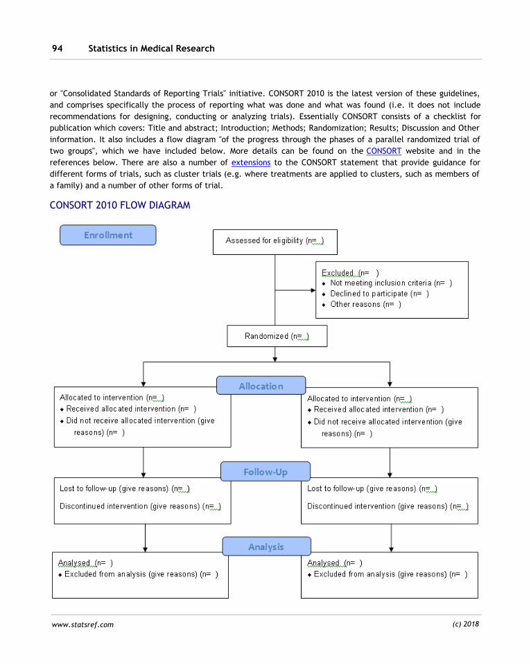
Statistics in Medical Research94

www.statsref.com (c) 2018

or "Consolidated Standards of Reporting Trials" initiative. CONSORT 2010 is the latest version of these guidelines,

and comprises specifically the process of reporting what was done and what was found (i.e. it does not include

recommendations for designing, conducting or analyzing trials). Essentially CONSORT consists of a checklist for

publication which covers: Title and abstract; Introduction; Methods; Randomization; Results; Discussion and Other

information. It also includes a flow diagram "of the progress through the phases of a parallel randomized trial of

two groups", which we have included below. More details can be found on the CONSORT website and in the

references below. There are also a number of extensions to the CONSORT statement that provide guidance for

different forms of trials, such as cluster trials (e.g. where treatments are applied to clusters, such as members of

a family) and a number of other forms of trial.

CONSORT 2010 FLOW DIAGRAM

Statistical data 95

www.statsref.com (c) 2018

As noted above, RCT's are by no means the only, or always the best or most appropriate framework for the

conduct of medical trials. In many instances the 'ideal' of a controlled experiment is not achievable, and many

other forms of research are also widely used — for example cohort studies and case-control studies. However, the

great advantage of RCT's is that they have been shown, within the strict confines of the trial in question, to be the

best means for avoiding bias and minimizing confounding effects, enabling conclusions regarding the differences

between outcomes to be made with a relatively high degree of confidence.

References and further reading

[ALT1] Altman D G, Bland J M (1991) Improving Doctors' Understanding of Statistics. J of the Royal Stat. Soc., A, 154(2), 223-267

[BH1] Bradford Hill A (1937) Principles of Medical Statistics. The Lancet, London (issued in various editions until 1971. Then

republished as "A Short Textbook of Medical Statistics" in 1977

[BH2] Bradford Hill A (1965) The Environment and Disease: Association or Causation? Proc. of the Royal Soc. of Medicine, 58,

295-300. A copy of this article is reproduced on Tufte's website: http://www.edwardtufte.com/tufte/hill

[CAM1] Campbell M J, Machin D, Walters S J (2007) Medical Statistics : A Textbook for the Health Sciences. 4th Ed., John Wiley

& Sons Ltd, Chichester

[ERC1] Ercan I, Berna Y, Yang Y, Ozkaya G, Cangur S, Ediz B , Kan I (2007) Misuage of Statistics in Medical research. Eur. J of

Gen. Med., 4(3), 128-134

[EVA1] Evans A S (1976) Causation and Disease: The Henle-Koch Postulates Revisited. Yale J Biol Med., 49(2), 175-195

[GR1] Greenland S, Pearl J, Robins J M (1999) Causal Diagrams for Epidemiologic Research, Epidemiology,10(1), 37-48

[MRC1] Medical Research Council (1948) Streptomycin treatment of pulmonary tuberculosis. BMJ, 4582, 769-782

[PH1] Phillips C V, Goodman K J (2004) The missed lessons of Sir Austin Bradford Hill. Epidemiologic Perspectives & Innovations,

1(3)

[ROT1] Rothman K J, Greenland S, Lash T L eds. (2008) Modern Epidemiology. 3rd Ed., Lippincott Williams & Wilkins

[OLS1] Olson S H, Voigt L F, Begg C B, Weiss N S (2002) Reporting participation in case-control studies. Epidemiology,13(2),123-6

STROBE (Strengthening the Reporting of Observational studies in Epidemiology): http://www.strobe-statement.org/

CONSORT (Consolidated Standards of Reporting Trials) encompasses various initiatives to alleviate the problems arising from

inadequate reporting of randomized controlled trials (RCTs): http://www.consort-statement.org

EQUATOR Network: http://www.equator-network.org/

Wikipedia: Randomized controlled trials: http://en.wikipedia.org/wiki/Randomized_controlled_trial

2.7.2.1 Randomized controlled trials

The randomized controlled trial (RCT) is generally accepted as the preferred approach to conducting a wide

variety of medical trials and is a central technique in the broader field of evidence-based medicine. The

advantages of the approach are many, but in particular they have been shown to be very effective in controlling

for selection bias and confounding, which other procedures may fail to achieve. In order to explain the central

ideas behind RCTs, we start by providing a brief description below of the steps involved in the very first RCT,

which was designed to determine the effectiveness of a new treatment for tuberculosis (TB).

The first step when designing an RCT is to carefully define the problem to be studied. Ideally this definition should

be easily understood and as narrow as is practical. In the British Medical Research Council's (MRC) study of

tuberculosis treatments in the late 1940s, the trial (of the effectiveness of streptomycin as a treatment) was

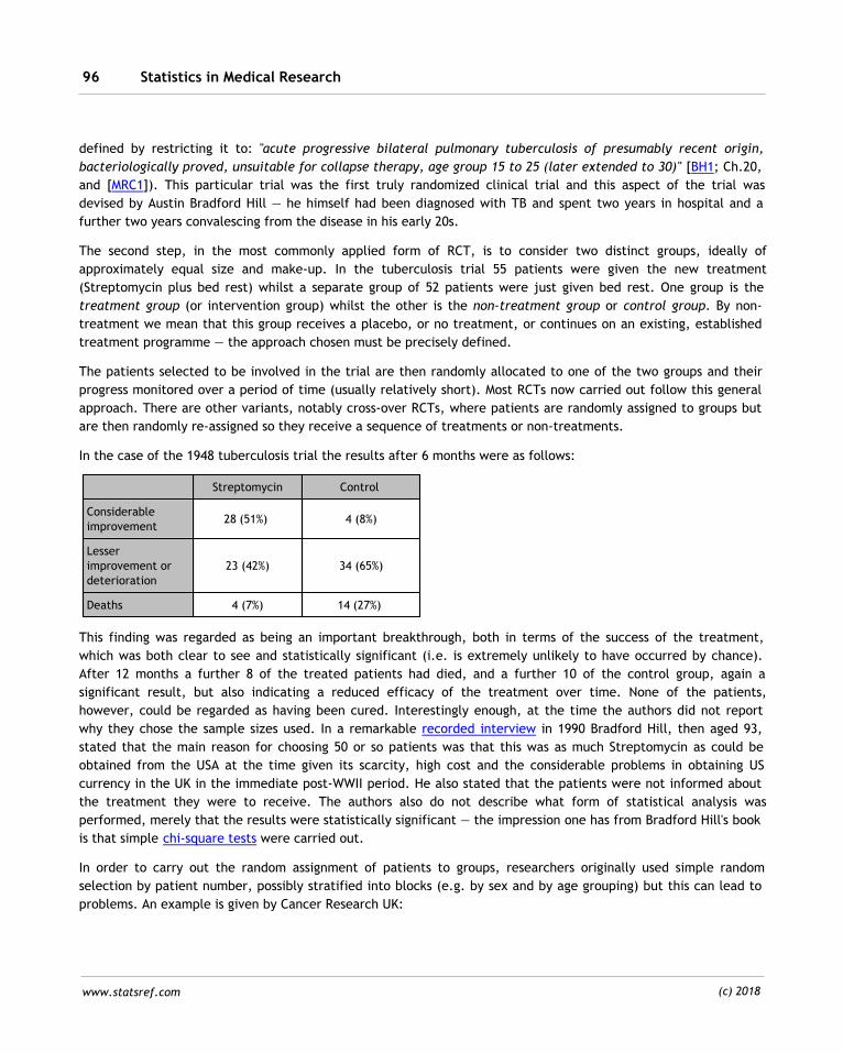
Statistics in Medical Research96

www.statsref.com (c) 2018

defined by restricting it to: "acute progressive bilateral pulmonary tuberculosis of presumably recent origin,

bacteriologically proved, unsuitable for collapse therapy, age group 15 to 25 (later extended to 30)" [BH1; Ch.20,

and [MRC1]). This particular trial was the first truly randomized clinical trial and this aspect of the trial was

devised by Austin Bradford Hill — he himself had been diagnosed with TB and spent two years in hospital and a

further two years convalescing from the disease in his early 20s.

The second step, in the most commonly applied form of RCT, is to consider two distinct groups, ideally of

approximately equal size and make-up. In the tuberculosis trial 55 patients were given the new treatment

(Streptomycin plus bed rest) whilst a separate group of 52 patients were just given bed rest. One group is the

treatment group (or intervention group) whilst the other is the non-treatment group or control group. By non-

treatment we mean that this group receives a placebo, or no treatment, or continues on an existing, established

treatment programme — the approach chosen must be precisely defined.

The patients selected to be involved in the trial are then randomly allocated to one of the two groups and their

progress monitored over a period of time (usually relatively short). Most RCTs now carried out follow this general

approach. There are other variants, notably cross-over RCTs, where patients are randomly assigned to groups but

are then randomly re-assigned so they receive a sequence of treatments or non-treatments.

In the case of the 1948 tuberculosis trial the results after 6 months were as follows:

Streptomycin Control

Considerable

improvement 28 (51%) 4 (8%)

Lesser

improvement or

deterioration

23 (42%) 34 (65%)

Deaths 4 (7%) 14 (27%)

This finding was regarded as being an important breakthrough, both in terms of the success of the treatment,

which was both clear to see and statistically significant (i.e. is extremely unlikely to have occurred by chance).

After 12 months a further 8 of the treated patients had died, and a further 10 of the control group, again a

significant result, but also indicating a reduced efficacy of the treatment over time. None of the patients,

however, could be regarded as having been cured. Interestingly enough, at the time the authors did not report

why they chose the sample sizes used. In a remarkable recorded interview in 1990 Bradford Hill, then aged 93,

stated that the main reason for choosing 50 or so patients was that this was as much Streptomycin as could be

obtained from the USA at the time given its scarcity, high cost and the considerable problems in obtaining US

currency in the UK in the immediate post-WWII period. He also stated that the patients were not informed about

the treatment they were to receive. The authors also do not describe what form of statistical analysis was

performed, merely that the results were statistically significant — the impression one has from Bradford Hill's book

is that simple chi-square tests were carried out.

In order to carry out the random assignment of patients to groups, researchers originally used simple random

selection by patient number, possibly stratified into blocks (e.g. by sex and by age grouping) but this can lead to

problems. An example is given by Cancer Research UK:

Statistical data 97

www.statsref.com (c) 2018

"it is possible to be biased without realizing it. For example, if a new treatment has quite bad side effects,

the doctors running the trial might subconsciously avoid putting sicker patients into the group having the new

treatment. So as the trial went on, the control group would have more and more of the sickest patients in it.

The people in the new treatment group would then do better than the control group. So, when the trial

results come out, the new treatment would [incorrectly] look as if it works better than the standard

treatment."

To avoid such problems a system known as blinding is applied. In blind trials one or more parties are unaware of

the assignment of treatments. For example, in a so-called single-blind trial the individual receiving the treatment

is not made aware whether the treatment they are being given is an existing treatment, a new treatment or a

placebo (i.e. a tablet or preparation that is not a drug at all and has no effect on the patient). In double-blind

trials neither the experimenter nor the patient know which treatment has been assigned to which patient

(treatments are coded) thereby minimizing the risk of any influence the experimenter may have on the

experiment. Unfortunately this terminology is not uniformly applied, leading to current recommendations to

describe in detail the kind of blinding applied (if any), even extending to those involved in analysis and

interpretation of the results.

Whilst the RCT procedure described above appears simple and straightforward, it does have numerous difficulties.

Determining the appropriate sample size to use can be problematic, especially in the case of rarer conditions

and/or where suitable triallists are simply not available in the location or at the period of time required (see the

earlier discussion on sample size, and in particular, the Salk Polio vaccine trials of 1954). The cost of conducting

such trials may be high, and if the trial is interrupted during its structured program, or there are problems with

adverse effects or triallists dropping out, how are the results to be interpreted? Some treatments are not

amenable to such form of trial, for example those requiring specific actions or exercises by participants. Sample

size determination can be difficult and it may be impossible to obtain the desired numbers in each group and

stratum or the required sample size if far larger than is achievable within time and cost constraints. There are

also often ethical problems — for example, should a particular treatment that is thought to be very promising be

withheld from very sick patients? (see further, the Declaration of Helsinki).

References

[BH1] Bradford Hill A (1937) Principles of Medical Statistics. The Lancet, London (issued in various editions until 1971. Then

republished as "A Short Textbook of Medical Statistics" in 1977

[MRC1] Medical Research Council (1948) Streptomycin treatment of pulmonary tuberculosis. BMJ, 4582, 769-782

Wikipedia: Randomized controlled trials: http://en.wikipedia.org/wiki/Randomized_controlled_trial

2.7.2.2 Case-control studies

Case-control studies involve investigations that are essentially retrospective in nature, since they involve the

study of patients who have acquired a disease or condition, and comparing these cases with so-called 'controls'

whose profile is similar to the cases. By similar we mean that the controls have not exhibited the condition under

investigation but have considerable similarities with those who have — for example, they have the same age/sex

mix, they live in the same area, do similar work, attended similar schools etc. In some instances case-control

studies involve multiple control groups, but more typically there is one group of cases and another of controls. In

other instances multiple diseases that affect cases, or different levels of severity of cases, are analyzed

simultaneously, which obviously complicates the design. As with other forms of medical research procedures, we

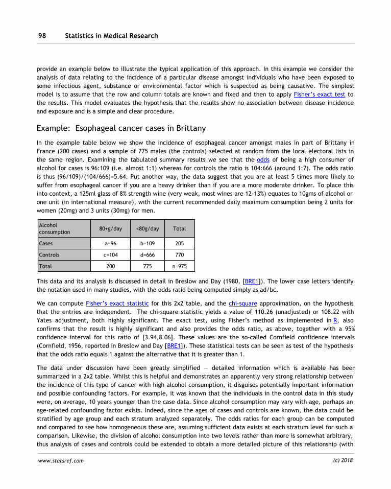
Statistics in Medical Research98

www.statsref.com (c) 2018

provide an example below to illustrate the typical application of this approach. In this example we consider the

analysis of data relating to the incidence of a particular disease amongst individuals who have been exposed to

some infectious agent, substance or environmental factor which is suspected as being causative. The simplest

model is to assume that the row and column totals are known and fixed and then to apply Fisher’s exact test to

the results. This model evaluates the hypothesis that the results show no association between disease incidence

and exposure and is a simple and clear procedure.

Example: Esophageal cancer cases in Brittany

In the example table below we show the incidence of esophageal cancer amongst males in part of Brittany in

France (200 cases) and a sample of 775 males (the controls) selected at random from the local electoral lists in

the same region. Examining the tabulated summary results we see that the odds of being a high consumer of

alcohol for cases is 96:109 (i.e. almost 1:1) whereas for controls the ratio is 104:666 (around 1:7). The odds ratio

is thus (96/109)/(104/666)=5.64. Put another way, the data suggest that you are at least 5 times more likely to

suffer from esophageal cancer if you are a heavy drinker than if you are a more moderate drinker. To place this

into context, a 125ml glass of 8% strength wine (very weak, most wines are 12-13%) equates to 10gms of alcohol or

one unit (in international measure), with the current recommended daily maximum consumption being 2 units for

women (20mg) and 3 units (30mg) for men.

Alcohol

consumption80+g/day <80g/day Total

Cases a=96 b=109 205

Controls c=104 d=666 770

Total 200 775 n=975

This data and its analysis is discussed in detail in Breslow and Day (1980, [BRE1]). The lower case letters identify

the notation used in many studies, with the odds ratio being computed simply as ad/bc.

We can compute Fisher’s exact statistic for this 2x2 table, and the chi-square approximation, on the hypothesis

that the entries are independent. The chi-square statistic yields a value of 110.26 (unadjusted) or 108.22 with

Yates adjustment, both highly significant. The exact test, using Fisher’s method as implemented in R, also

confirms that the result is highly significant and also provides the odds ratio, as above, together with a 95%

confidence interval for this ratio of [3.94,8.06]. These values are the so-called Cornfield confidence intervals

(Cornfield, 1956, reported in Breslow and Day [BRE1]). These statistical tests can be seen as test of the hypothesis

that the odds ratio equals 1 against the alternative that it is greater than 1.

The data under discussion have been greatly simplified — detailed information which is available has been

summarized in a 2x2 table. Whilst this is helpful and demonstrates an apparently very strong relationship between

the incidence of this type of cancer with high alcohol consumption, it disguises potentially important information

and possible confounding factors. For example, it was known that the individuals in the control data in this study

were, on average, 10 years younger than the case data. Since alcohol consumption may vary with age, perhaps an

age-related confounding factor exists. Indeed, since the ages of cases and controls are known, the data could be

stratified by age group and each stratum analyzed separately. The odds ratios for each group can be computed

and compared to see how homogeneous these are, assuming sufficient data exists at each stratum level for such a

comparison. Likewise, the division of alcohol consumption into two levels rather than more is somewhat arbitrary,

thus analysis of cases and controls could be extended to obtain a more detailed picture of this relationship (with

Statistical data 99

www.statsref.com (c) 2018

or without age-based stratification). Clearly as the number of levels and strata are increased, so the cell entries

will diminish and without relatively large samples the scope for detailed breakdowns of this type will be limited.

Also, the Fisher test for tables with more than a 2x2 arrangement is typically implemented using simulation

methods. Finally, the dataset also collected information on tobacco consumption — perhaps the strong

relationship observed for alcohol consumption is actually not causative but indicative of lifestyle. By including

tobacco consumption levels as well as alcohol consumption, for cases and controls, estimates of relative risks (by

age group) can be obtained.

For the above analysis controls were not tightly matched to cases — for example, their age profile, and possible

other important factors, were not matched. In some instances carefully matched controls can be identified which

generally increases the power of the analysis. Typically more controls than cases are identified, and analysis

proceeds either by taking the first or a randomly selected matched control from a set, or by combining the

controls as if they represented a single individual. Procedures for analyzing matched controls, which are variants

of those described above, are covered in Breslow and Day [BRE1]. For more complex problems it may be

preferable to apply techniques based on logistic regression, with unmatched or matched samples.

References

[BRE1] Breslow N E, Day N E (1980) Statistical Methods in Cancer Research: Volume 1 — The Analysis of Case-Control studies.

IARC Scientific Publications No.32, World Health Organization, IARC Lyon

[BRE2] Breslow N E, Day N E (1987) Statistical Methods in Cancer Research: Volume 2 — The Design and Analysis of Cohort

Studies. IARC Scientific Publications No.82, World Health Organization, IARC Lyon

[MAN1] Mantel N, Haenszel W. (1959) Statistical aspects of the analysis of data from retrospective studies of disease. Journal of

the National Cancer Institute, 22, 719-748

2.7.2.3 Cohort studies

Cohort studies primarily consist of the selection of a group of individuals (the cohort) and studying aspects of their

development over many years, possibly several decades. In particular, disease incidence and mortality of the

cohort are studied. As with case-control studies and randomized control trials, the unit of analysis is the

individual, i.e. macro-level relationships amongst groups (i.e. population correlation or ecological studies) are not

the basis for research in any of these methods. At the start of the process members of the cohort are recruited,

generally with a carefully constructed profile that is designed to embrace the study population of interest, and

detailed interviews are conducted to learn relevant information about their background, health history, lifestyle

etc. Further interviews and/or questionnaires are then conducted every few years over the course of the project.

The great advantage of this approach, which is known as a prospective cohort study, is that information about the

individuals is well documented and all subsequent disease incidence is recorded, in many cases up to eventual

death. However, this may take a long time and may exhibit only a few cases of the specific disease or diseases of

interest unless a very large cohort is used, which increases the cost and complexity of the project. Retrospective

or historical cohort studies seek to identify a group or cohort with known exposure to a suspected agent, and then

attempt to reconstruct the history of exposure and related data in order to obtain an understanding about current

disease incidence and mortality patterns. This approach has the advantage that data is available relatively quickly

and without excessive expense, may be the only possible approach (for example if a substance or circumstance

not longer applies), but is subject to many practical problems — notably missing data and recall problems.

Statistics in Medical Research100

www.statsref.com (c) 2018

Prospective cohort studies may be compared with a case-control approach, for which cases are selected from

those with a disease of interest, controls are selected, and the two datasets are compared. For example, in the

very first major cohort study, that of British Doctors commencing in 1951, some 34,440 male doctors were

recruited to the study, and after 20 years total incidence of lung case deaths was 441. This compares with a case-

control study that commenced in 1948 and was completed in 1952, with 4342 people being involved and 1488

being lung cancer cases. The advantages of case-control studies for identifying possible relationships of

importance is clear, and they are much faster and typically less costly to conduct, but they are severely limited in

the degree of confidence in the nature of the relationship and by their reliance on recalled information. With a

cohort study an improved understanding of the relationship between exposure, lifestyle and outcomes is possible,

including effects not previously identified. For example, in the British Doctors study it was apparent, after 20

years, that the death rate amongst heavy smokers from all causes was twice that of non-smokers. In this example

the level of long-term successful follow-up of the cohort was very high, but in other studies this has not been the

case. Unless the results are available for a very high proportion of the cohort, the validity of the results may be

called into question.

In summary, Breslow and Day [BRE2] identify the following advantages of cohort studies as compared with case-

control studies. Cohort studies:

· Give a wider picture of the health hazards associated with a given exposure

· Eliminate most forms of selection bias and recall bias

· Are often the only practical option where exposure to specific agents (e.g. suspected hazardous industrial

chemicals) is rare

· In addition to detailed interviews or questionnaires, medical tests can be carried out at the start of the cohort

study that may aid interpretation of outcomes, for example in terms of prior susceptibility to certain conditions

· Repeated measurements over the lifetime of the study may be possible and important — for example,

measurements of specific chemicals present in blood or urine samples

· Absolute risk rates are obtained for the cohort, as opposed to relative risk rates for case-control studies.

However, if the cohort is not representative of the broader population these risk estimates cannot be extended

without reservation

Historically, most attention has been focused on mortality whereas more recently interest has been shown in a

combination of severity of various conditions (e.g. chronic illnesses) and the detail of dose-response relationships,

both of which are more demanding in terms of data (e.g. obtaining an understanding of multi-factor effects) and

analytical methods. For dose-response analysis much emphasis is placed on fitting alternative models to data

collected over time, using various forms of time series analysis to help model, and thereby predict safe exposure

or dose levels in absolute and temporal terms.

References

[BRE1] Breslow N E, Day N E (1980) Statistical Methods in Cancer Research: Volume 1 — The Analysis of Case-Control studies.

IARC Scientific Publications No.32, World Health Organization, IARC Lyon

[BRE2] Breslow N E, Day N E (1987) Statistical Methods in Cancer Research: Volume 2 — The Design and Analysis of Cohort

Studies. IARC Scientific Publications No.82, World Health Organization, IARC Lyon