Statistical Alignment Models for Translational Equivalence · Statistical Alignment Models for...
185
Statistical Alignment Models for Translational Equivalence Bing Zhao CMU-LTI-07-012 Language Technologies Institute School of Computer Science Carnegie Mellon University 5000 Forbes Ave. Pittsburgh, PA 15213 www.lti.cs.cmu.edu Thesis Committee: Alex Waibel, Carnegie Mellon University Stephan Vogel, Carnegie Mellon University Eric Xing, Carnegie Mellon University Kishore Papineni, Yahoo! Research Submitted in partial fulfillment of the requirements for the degree of Doctor of Philosophy In Language and Information Technologies c 2007, Bing Zhao
Transcript of Statistical Alignment Models for Translational Equivalence · Statistical Alignment Models for...

Statistical Alignment Models forTranslational Equivalence
Bing Zhao
CMU-LTI-07-012
Language Technologies InstituteSchool of Computer ScienceCarnegie Mellon University
5000 Forbes Ave. Pittsburgh, PA 15213www.lti.cs.cmu.edu
Thesis Committee:
Alex Waibel, Carnegie Mellon UniversityStephan Vogel, Carnegie Mellon UniversityEric Xing, Carnegie Mellon UniversityKishore Papineni, Yahoo! Research
Submitted in partial fulfillment of the requirementsfor the degree of Doctor of Philosophy
In Language and Information Technologies
c©2007, Bing Zhao


This dissertation is dedicated to my parents.
iii

Abstract
The ever-increasing amount of parallel data opens a rich resource to multilingual natural lan-
guage processing, enabling models to work on various translational aspects like detailed hu-
man annotations, syntax and semantics. With efficient statistical models, many cross-language
applications have seen significant progresses in recent years, such as statistical machine trans-
lation, speech-to-speech translation, cross-lingual information retrieval and bilingual lexicog-
raphy. However, the current state-of-the-art statistical translation models rely heavily on the
word-level mixture models — a bottleneck, which fails to represent the rich varieties and depen-
dencies in translations. In contrast to word-based translations, phrase-based models are more
robust in capturing various translation phenomena than the word-level (e.g., local word reorder-
ing), and less susceptive to the errors from preprocessing such as word segmentations and tok-
enizations. Leveraging phrase level knowledge in translation models is challenging yet reward-
ing: it also brings significant improvements on translation qualities. Above the phrase-level are
the sentence- and document- levels of translational equivalences, from which topics can be fur-
ther abstracted as hidden concepts to govern the bilingual generative process of sentence-pair,
phrase-pair or word-pair sequences. The modeling of hidden bilingual concepts also enables
the learning to share parameters, and thus, endows the models with the abilities of learning to
translate.
Learning translational equivalence is the fundamental building block for machine transla-
tions. This thesis delves into learning statistical alignment models for translational equivalences
v
vi
at various levels: documents, sentences and words. Specific attention will be devoted to intro-
ducing hidden concepts in modeling translation. Models, such as Inner-Outer Bracket models,
are designed to model the dependency between phrases and the words inside of them; bilin-
gual concepts are generalized to integrate topics for translation. In particular, Bilingual Topic-
AdMixture (BiTAM) models are proposed to formulate the semantic correlations among words
and sentences. BiTAM is shown to be a general framework, which can generalize over different
traditional alignment models with ease. In this thesis, IBM Model-1 and HMM are embedded
in BiTAM; BiTAM 1-3 and HM-BiTAM are designed with tractable learning and inference al-
gorithms. Improvements of word alignment accuracies are observed, and also better machine
translation qualities are obtained.
The models, proposed in this thesis, have also been applied successfully in the past a few
statistical machine translation evaluations for the CMU-SMT team, especially for the scenarios
of Chinese-to-English.
Keywords: BiTAM, AdMixture Models, Graphical Models, Machine Translation, Genera-
tive Models, Sentence-Alignment, Document-Alignment, Word-Alignment, Phrase-Extraction,
Speech-Translation, GALE, NIST, and IWSLT.
Acknowledgements
As I came close to the finishing-line, I could not help appreciating the people who helped me so
significantly, in both my research and in my life in Pittsburgh, over the past six years of studies
at Carnegie Mellon University.
First of all, it is my advisor Alex Waibel, who brought me to the field of statistical machine
translation — a field full of fun and challenges. Without his patient guidance over the years,
I could not have had a chance to step into this field, and make any progress. My co-advisor
Stephan Vogel, helped me to start from the sentence-alignment for machine translation, and
later, he led me into the more involved hands-on projects of improving the machine translation
models. My co-advisor, Eric P. Xing, helped me to sort out the problems of machine translations
in a clean way, which provided many insights to improve the translation models. My supervisor
Kishore Papineni, a great advisor and a friend, provided with me not only ideas to improve trans-
lations but also a great of help in shaping my research work from his many years of experiences
in machine translation. I owned so much to their insightful advices, tremendous help and great
patience. Without their help, I could not have achieved anything. I also thank Noah Smith and
Rebecca Hwa, who spent a lot of time in discussing and refining my research works. I want
to thank the LTI faculties Jaime Carbonell, Tanja Schultz, Eric Nyberg, William Cohen, John
Lafferty, Jamie Callan, and Alan Black. The education I received at LTI is very helpful in my
research. Many thanks to all of them!
In the past six years at InterAct CMU, I feel lucky to Have a few nice labmates. First, my
vii

Acknowledgements viii
five-year’s officemate, Matthias Eck, had been sharing the office with me for more than five
years and helped me in many aspects. I feel very lucky to have him as my officemate. InterAct
is a very active group. My labmates include Nguyen, Linh, Stan, Wilson, Ian, Roger, Choir, Qin,
Yue, Silja, Joy, Mahamed, Anthony, Nimish, Sanjika, Paisarn, Ashish and Andreas. Thanks a
lot for all of their help of my work at ISL. Also, it was my great honor to make quite a few
super friends, who added a lot of colors to my life in Pittsburgh. I want to express my sincere
thanks to Liu Li, Jie Lu, Chun Jin, Luo Si, Hui (Grace) Yang, Ting Liu, Ting Chen, Chun Wang,
Huaiwei Liao, Kevin Gimpel, Jae Dong Kim, Jeongwoo Ko, John Kominek, Kornel Laskowski,
Fan Li, Jiazhi Ou, Wen Wu, Jun Yang, Rong Zhang, Yanhui Zhang, Rong Yan, Ariadna Font
Llitjs, Yanjun Qi, Hua Yu, Rong Jin, Jerry Zhu, and Klaus Zechner. Their friendship matters a
lot. I want to thank Lisa Mauti, Stacey Young, Mary Jo Bensasi, April Murphy, Brooke Hyatt
and Linda Hager, and Radha Rao for their kind help.
At last, I want to express my sincere thanks to my parents, who brought me up, and have been
supporting me with love over the years far away from them.
Contents
1 Introduction 1
1.1 Machine Translation . . . . . . . . . . . . . . . . . . . . . . . . . . . . . . . 1
1.2 Towards an Ideal of Translation . . . . . . . . . . . . . . . . . . . . . . . . . . 2
1.3 The Organization of This Thesis . . . . . . . . . . . . . . . . . . . . . . . . . 3
2 Literature Review 5
2.1 Approaches to Mining Parallel Data . . . . . . . . . . . . . . . . . . . . . . . 7
2.2 Approaches to Translation Models . . . . . . . . . . . . . . . . . . . . . . . . 9
2.2.1 Generative Models . . . . . . . . . . . . . . . . . . . . . . . . . . . . 9
2.2.2 Log-Linear Models . . . . . . . . . . . . . . . . . . . . . . . . . . . . 11
2.2.3 Syntax-based Models . . . . . . . . . . . . . . . . . . . . . . . . . . . 13
2.2.4 Other Models . . . . . . . . . . . . . . . . . . . . . . . . . . . . . . . 16
2.3 Datasets and Evaluations . . . . . . . . . . . . . . . . . . . . . . . . . . . . . 17
3 Mining Translational Equivalences 19
3.1 Language Pairs and Resources . . . . . . . . . . . . . . . . . . . . . . . . . . 19
3.2 Full-text Bilingual Document Alignment Models . . . . . . . . . . . . . . . . 21
3.2.1 Pseudo-Query Models via Standard IR . . . . . . . . . . . . . . . . . . 22
3.2.2 Full-Text Alignment Model-A . . . . . . . . . . . . . . . . . . . . . . 23
3.2.3 Full-Text Alignment Model-B . . . . . . . . . . . . . . . . . . . . . . 25
ix
CONTENTS x
3.2.4 Refined Full-Text Alignment Models . . . . . . . . . . . . . . . . . . 25
3.3 Bilingual Sentence Alignment from Comparable Documents . . . . . . . . . . 28
3.4 Experiments . . . . . . . . . . . . . . . . . . . . . . . . . . . . . . . . . . . . 30
3.4.1 Mining from Web-collection for Comparable Documents . . . . . . . . 30
3.4.2 Refined Full-Text Alignment Models . . . . . . . . . . . . . . . . . . 32
3.4.3 Mining from Noisy Comparable Corpora: XinHua News Stories . . . . 34
3.4.4 Mining from High-Quality Parallel Corpora: FBIS Corpora . . . . . . 36
3.4.5 Integrating Multiple Feature Streams for Selecting Parallel Sentence-Pairs 37
3.5 Discussions and Summary . . . . . . . . . . . . . . . . . . . . . . . . . . . . 39
4 Leveraging Bilingual Feature Streams 40
4.1 Word Alignment Models . . . . . . . . . . . . . . . . . . . . . . . . . . . . . 41
4.2 Bilingual Word Spectrum Clusters . . . . . . . . . . . . . . . . . . . . . . . . 42
4.2.1 From Monolingual to Bilingual . . . . . . . . . . . . . . . . . . . . . 44
4.2.2 Bilingual Word Spectral Clustering . . . . . . . . . . . . . . . . . . . 45
4.2.3 A Bi-Stream HMM . . . . . . . . . . . . . . . . . . . . . . . . . . . . 48
4.3 From Word to Phrase Alignment Models . . . . . . . . . . . . . . . . . . . . . 49
4.3.1 Inside of a Block . . . . . . . . . . . . . . . . . . . . . . . . . . . . . 51
4.3.2 Outside of a Block . . . . . . . . . . . . . . . . . . . . . . . . . . . . 56
4.3.3 A Log-linear Model . . . . . . . . . . . . . . . . . . . . . . . . . . . 59
4.4 Experiments . . . . . . . . . . . . . . . . . . . . . . . . . . . . . . . . . . . . 60
4.4.1 Extended HMM with Bilingual Word Clusters . . . . . . . . . . . . . 60
4.4.2 Spectral Analysis for Co-occurrence Matrix . . . . . . . . . . . . . . . 61
4.4.3 Bilingual Spectral Clustering Results . . . . . . . . . . . . . . . . . . 62
4.4.4 Bi-Stream HMM for Word Alignment . . . . . . . . . . . . . . . . . . 66
4.4.5 Comparing with Symmetrized Word Alignments from IBM Model 4 . . 67
4.4.6 Evaluations of Log-Linear Phrase Alignment Models . . . . . . . . . . 68
CONTENTS xi
4.4.7 Evaluations of Both Word and Phrase Alignment Models in GALE-2007 73
4.5 Discussions and Summary . . . . . . . . . . . . . . . . . . . . . . . . . . . . 75
5 Modeling Hidden Blocks 78
5.1 Segmentation of Blocks . . . . . . . . . . . . . . . . . . . . . . . . . . . . . . 79
5.2 Inner-Outer Bracketing Models with Hidden Blocks . . . . . . . . . . . . . . . 80
5.2.1 Model-A: Lexicalized Inner-Outer . . . . . . . . . . . . . . . . . . . . 81
5.2.2 Model-B: Lexicalized Width-Center . . . . . . . . . . . . . . . . . . . 81
5.2.3 Predicting “NULL” Word Alignment using Context . . . . . . . . . . . 83
5.2.4 A Constrained Max-Posterior Inference . . . . . . . . . . . . . . . . . 84
5.3 Experimental Evaluation . . . . . . . . . . . . . . . . . . . . . . . . . . . . . 85
5.3.1 Baselines . . . . . . . . . . . . . . . . . . . . . . . . . . . . . . . . . 86
5.3.2 Improved Word Alignment via Blocks . . . . . . . . . . . . . . . . . . 86
5.3.3 Improved Word Blocks via Alignment . . . . . . . . . . . . . . . . . . 87
5.4 Discussions and Summary . . . . . . . . . . . . . . . . . . . . . . . . . . . . 88
6 Modeling Hidden Concepts in Translation 89
6.1 Notations and Terminology . . . . . . . . . . . . . . . . . . . . . . . . . . . . 91
6.2 Admixture of Topics for Parallel Data . . . . . . . . . . . . . . . . . . . . . . 92
6.2.1 Bilingual AdMixture Model: BiTAM Model-1 . . . . . . . . . . . . . 93
6.2.2 The Sampling Scheme for BiTAM Model-1 . . . . . . . . . . . . . . . 93
6.2.3 Inference and Learning for BiTAM Model-1 . . . . . . . . . . . . . . 97
6.3 Extensions to the Bilingual Topic AdMixture Models . . . . . . . . . . . . . . 100
6.3.1 BiTAM Model-2: Word-level Topics . . . . . . . . . . . . . . . . . . . 101
6.3.2 Extension with Monolingual LM: BiTAM Model-3 . . . . . . . . . . . 102
6.4 HM-BiTAM: Extensions along the “A-chain” . . . . . . . . . . . . . . . . . . 104
6.4.1 A Graphical Model of HMM for Word Alignment . . . . . . . . . . . 105
CONTENTS xii
6.4.2 From HMM to HM-BiTAM . . . . . . . . . . . . . . . . . . . . . . . 106
6.4.3 Sampling Scheme for HM-BiTAM Model-1 . . . . . . . . . . . . . . . 106
6.4.4 First-order Markov Dependency for Alignment . . . . . . . . . . . . . 108
6.4.5 Approximated Posterior Inference . . . . . . . . . . . . . . . . . . . . 109
6.5 Extensions to HM-BiTAM: Topics Sampled at Word-pair Level . . . . . . . . . 112
6.5.1 HM-BiTAM Model-2 . . . . . . . . . . . . . . . . . . . . . . . . . . . 112
6.5.2 Generative Scheme of HM-BiTAM Model-2 . . . . . . . . . . . . . . 112
6.5.3 Inference and Learning . . . . . . . . . . . . . . . . . . . . . . . . . . 114
6.5.4 Extension to HM-BiTAM: Leveraging Monolingual Topic-LM . . . . . 114
6.6 Inference of Word Alignment with BiTAMs . . . . . . . . . . . . . . . . . . . 116
6.7 Experiments . . . . . . . . . . . . . . . . . . . . . . . . . . . . . . . . . . . . 117
6.7.1 The Data . . . . . . . . . . . . . . . . . . . . . . . . . . . . . . . . . 117
6.7.2 Inside of the Topic-specific Lexicons . . . . . . . . . . . . . . . . . . 120
6.7.3 Extracting Bilingual Topics from HM-BiTAM . . . . . . . . . . . . . . 124
6.7.4 Improved Likelihood and Perplexity for BiTAMs . . . . . . . . . . . . 128
6.7.5 Evaluating Word Alignment . . . . . . . . . . . . . . . . . . . . . . . 132
6.7.6 Improving BiTAM Models with Boosted Lexicons . . . . . . . . . . . 136
6.7.7 Using HM-BiTAM Models for Word Alignment . . . . . . . . . . . . 137
6.7.8 Decoding MT04 Documents in Gale07 System . . . . . . . . . . . . . 139
6.7.9 Translations with HM-BiTAM . . . . . . . . . . . . . . . . . . . . . . 142
6.8 Discussion and Summary . . . . . . . . . . . . . . . . . . . . . . . . . . . . . 149
7 Summary of this Thesis 150
7.1 Survey of State-of-the-art Approaches . . . . . . . . . . . . . . . . . . . . . . 151
7.2 Modeling Alignments of Document Pairs and Sentence Pairs . . . . . . . . . . 151
7.3 Modeling Hidden Blocks . . . . . . . . . . . . . . . . . . . . . . . . . . . . . 152
7.4 Modeling Hidden Concepts . . . . . . . . . . . . . . . . . . . . . . . . . . . . 152
List of Figures
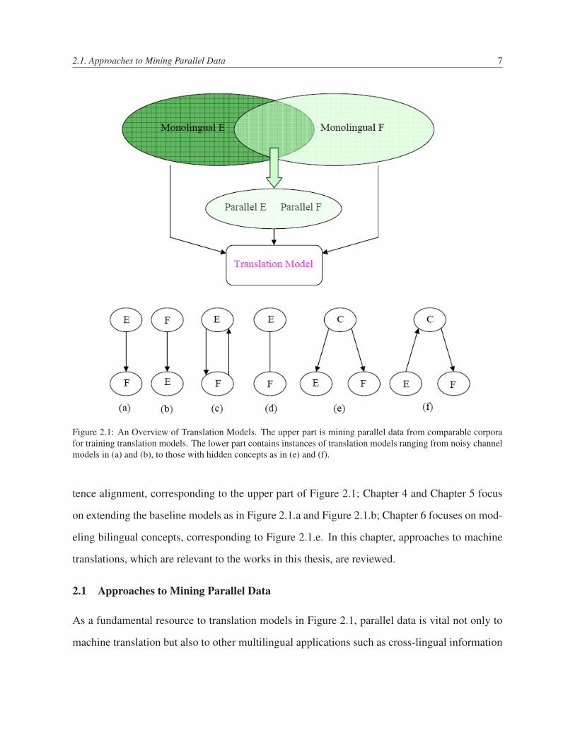
2.1 An Overview of Translation Models. The upper part is mining parallel data from
comparable corpora for training translation models. The lower part contains
instances of translation models ranging from noisy channel models in (a) and
(b), to those with hidden concepts as in (e) and (f). . . . . . . . . . . . . . . . 7
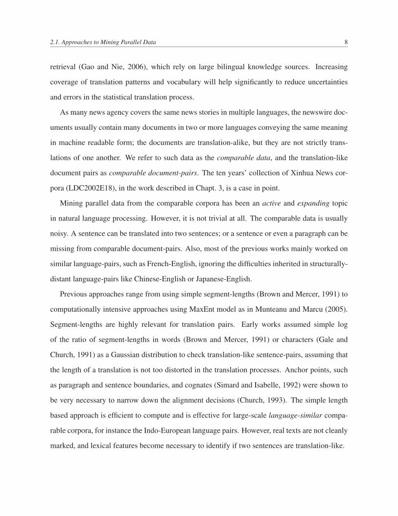
2.2 An Overview of Translation Models: “Vauquois pyramid” . . . . . . . . . . . 10
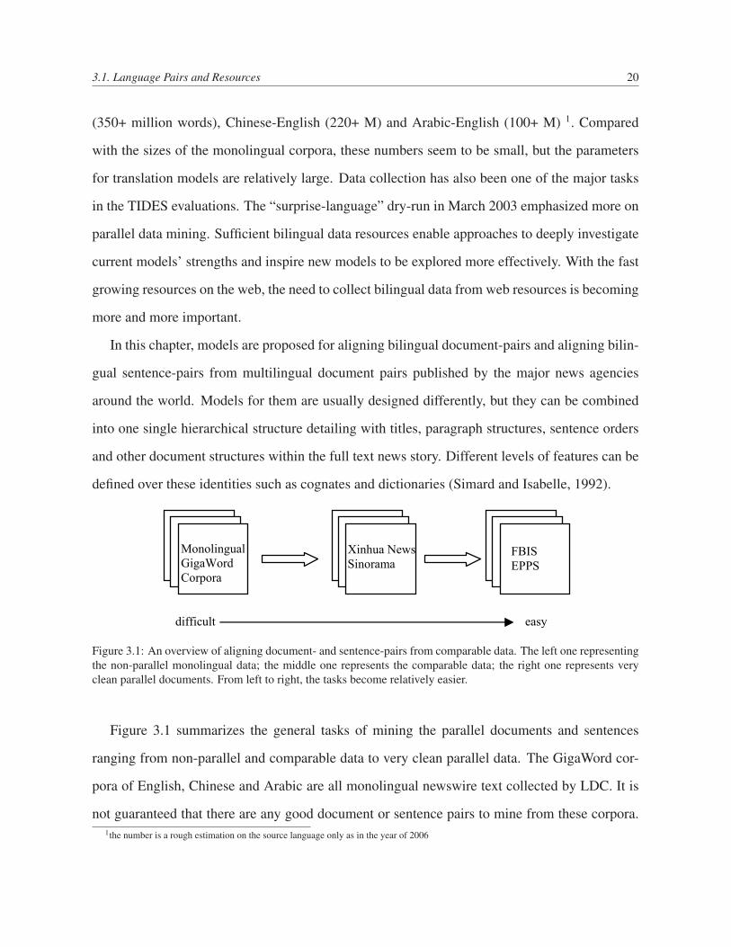
3.1 An overview of aligning document- and sentence-pairs from comparable data.
The left one representing the non-parallel monolingual data; the middle one rep-
resents the comparable data; the right one represents very clean parallel docu-
ments. From left to right, the tasks become relatively easier. . . . . . . . . . . 20
3.2 Seven Sentence Alignment Types in Dynamic Programming. . . . . . . . . . . 29
3.3 Cumulative percentage of parallel stories found at each rank for Known-Item
retrieval . . . . . . . . . . . . . . . . . . . . . . . . . . . . . . . . . . . . . . 31
4.1 A Baseline HMM for Word Alignment . . . . . . . . . . . . . . . . . . . . . . 42
4.2 A Bi-Stream HMM for Word Alignment . . . . . . . . . . . . . . . . . . . . . 42
4.3 Blocks with “width” and “centers” . . . . . . . . . . . . . . . . . . . . . . . . 50
4.4 The upper part is a trellis of an English trigram with maximum fertility of three
per English word. Dynamic programming is then carried out through the trellis,
as shown in the lower part. . . . . . . . . . . . . . . . . . . . . . . . . . . . . 53
xiii
LIST OF FIGURES xiv
4.5 Histogram of relative centers’ differences between oracle phrase pairs (blocks)
extracted from 627 human word-aligned parallel sentence pairs. . . . . . . . . 54
4.6 Ngram Bracketing: the sentence-pair is described as the matrix, and a block, rep-
resented by A segments the sentence-pair into four additional parts: B, C, D, E.
If the block is a good block, the remaining parts B, C, D, E should also maintain
good translation equivalences, esp. in terms of length and lexical aspects. . . . 57
4.7 Top-1000 Eigen Values of Co-occurrence Matrix . . . . . . . . . . . . . . . . 62
4.8 Histogram of cluster pairs (Fj, Ei) . . . . . . . . . . . . . . . . . . . . . . . . 65
4.9 ε-mirror with different settings . . . . . . . . . . . . . . . . . . . . . . . . . . 65
4.10 Word Alignment Over HMM Forward-Backward Iterations . . . . . . . . . . . 66
4.11 Clustered Feature Functions with Feature ID (FID). Each rectangle in the table
corresponds to one of the four clusters inferred from the standard K-means al-
gorithm. This clustering is based on all the blocks extracted from the training
data; each block is associated with a 11-dimension vector, corresponding to 11
feature functions. . . . . . . . . . . . . . . . . . . . . . . . . . . . . . . . . . 69
4.12 Pair-wise correlations among 11 feature functions; The color of each cell indi-
cates the correlation strength between two features. . . . . . . . . . . . . . . . 69
5.1 Parallel Sentence-Pair Segmentation by a Block . . . . . . . . . . . . . . . . . 80
LIST OF FIGURES xv
6.1 Graphical Model representations for (a) IBM Model-1 and (b) BiTAM Model-1.
Model parameter for IBM Model-1 in figure (a) is B = p(f |e), which is a simple
word-to-word translation lexicon; Model parameters for BiTAM Model-1 (in (b)
) are a set of K topic-specific lexicons: {Bk = p(f |e, z=k)} and a Dirichlet
prior parameter α. All the plates represent replicates. The outmost plate (M -
plate) represents M bilingual document-pairs, while the inner N -plate represents
the N repeated choice of topics for each sentence-pairs in the document; and the
inner J-plate represents J word-pairs within each sentence-pair. Shaded nodes
are observations; unshaded nodes are hidden variables. α and B are the corpus
level parameters. B, for BiTAM, is a three-dimensional matrix, representing a
set of topic-specific translation lexicons: {p(f |e, z)}. . . . . . . . . . . . . . . 95
6.2 Graphical Model representation of the variational distribution used to approxi-
mate the posteriors in Bilingual AdMixture Model-1. . . . . . . . . . . . . . . 98
6.3 (a) A graphical model representation of BiTAM Model-2 for Bilingual document-
and sentence-pairs. The topics are sampled at the level of each word-pair. (b) A
graphical model representation of BiTAM Model-3. The topics are sampled at
the sentence-pair level, and an additional topic specific unigram language model
is integrated to improve the inference for topics. . . . . . . . . . . . . . . . . 101
6.4 A graphical model representation of HMM for Bilingual data. The model param-
eters are the jump probability of βi,i′ = p(aj = i|aj−1 = i′) and a word-to-word
translation lexicon B = p(f |e). . . . . . . . . . . . . . . . . . . . . . . . . . 105
LIST OF FIGURES xvi
6.5 A graphical model representation of HM-BiTAM for Bilingual document- and
sentence-pairs. A node in the graph represents a random variable, and a hexagon
denotes a parameter. Un-shaded nodes are hidden variables. The square boxes
are “plates” that represent replicates of variables in the boxes. The outmost
plate (M -plate) represents M bilingual document-pairs, while the inner N -plate
represents the Nm sentences (each with its own topic z) in, say, document m.
The innermost I-plate represents the In words of the source sentence (i.e., the
length of the English sentence). . . . . . . . . . . . . . . . . . . . . . . . . . . 106
6.6 The embedded HMM transition network with special treatment of NULL word
in the target sentence. fj+1 and fj+2 are aligned to NULL words, of which the
pseudo positions are set to be the ones close to eajand eaj+3
, respectively. . . . 109
6.7 A graphical model representation of HM-BiTAM Model-2 for Bilingual document-
and sentence-pairs. The topics are sampled at the word-pair level instead of at
sentence-pair level as in HM-BiTAM Model-1. . . . . . . . . . . . . . . . . . 113
6.8 The graphical model representation of HM-BiTAM Model-1 with monolingual
English topic LM models. Circles represent random variables, hexagons denote
parameters, and observed variables are shaded. . . . . . . . . . . . . . . . . . 114
6.9 The sizes of topic-specific translation lexicons over variational EM iterations in
BiTAM Model-2. The global lexicon has 641,293 entries; BiTAM Model-2 leant
ten lexicons (ten topics) with an average size of 131,328 for one lexicon over 20
iterations. The largest one has 147,270 entries, and the smallest one has 114,749
entries. Overall each topic specific lexicon is much smaller than the global one.
Similar observations are obtained for all BiTAMs introduced so far. . . . . . . 121
6.10 Bilingual topics learned from parallel data. Both English topics and Chinese
topics are displayed. The English topics are highly parallel to those of Chinese
topics. . . . . . . . . . . . . . . . . . . . . . . . . . . . . . . . . . . . . . . . 126

LIST OF FIGURES xvii
6.11 Topic Assignments Inferred from HM-BiTAM Model-2 for training data. Each
document-pair has its own focus of content; most of the document-specific topic
assignments within a document-pair have modes, which are represented by the
peaks in the graph. . . . . . . . . . . . . . . . . . . . . . . . . . . . . . . . . 127
6.12 Comparison of likelihoods of data under different models. Top: HM-BiTAM
v.s. IBM Model-4; bottom: HM-BiTAM v.s. HMM. . . . . . . . . . . . . . . . 130
6.13 Experiments carried out using parallel corpora with up to 22.6-million (22.6 M)
Chinese words. the word alignment accuracy (F-measure) over different sizes of
training data, comparing with baseline HMMs. . . . . . . . . . . . . . . . . . 138
6.14 Experiments carried out using parallel corpora with up to 22.6-million (23 M)
Chinese words. Case-insensitive BLEU over MT03 (MER tuned on MT02) in a
monotone SMT decoder. . . . . . . . . . . . . . . . . . . . . . . . . . . . . . 138
6.15 Topic Assignments Inferred from HM-BiTAM Model-2. . . . . . . . . . . . . 140
6.16 Topic Assignments for Doc:ZBN20040310.001, which is mainly on Keynesian-
ism implemented in US, and its influence on the economic developments of
China and India. Topics are from HM-BiTAM Model-1, in which topics are
sampled at sentence level. The topics for a sentence are limited. The topic-
switches are well represented for this editorial style document: the first four sen-
tences are about US policy encoding Keynesianism, sent-5 and sent-6 are about
results within US; sent-7/8/9 are about global influence of this policy esp. related
China and India; the last sentence is, however, to correct the miss-understanding
of people’s impression on China. . . . . . . . . . . . . . . . . . . . . . . . . 142
6.17 Topic Assignments for Doc:ZBN20040310.001, HM-BiTAM Model-2 was learned
with 20 topics. Five topics are active for this document. . . . . . . . . . . . . . 143

LIST OF FIGURES xviii
6.18 Oracle Experiment with ground truth: topic Assignments for MT2004. Doc-
uments were paired with their human translations. HM-BiTAM Model-2 was
learned with 10 topics. Topics are sampled at word level. The topic-specific
lexicons are then mixed for each word-pair within the document. . . . . . . . 144
6.19 Practical Experiment: topic Assignments for MT2004., HM-BiTAM Model-2
was learned with 10 topics. Testing document is paired with the top-1 baseline
translation hypotheses. Topic assignment is inferred with HM-BiTAM Model-2;
topic-specific lexicons are then mixed for each word-pair within the document. 145
List of Tables
3.1 Mean reciprocal rank and known items at the raw rank. . . . . . . . . . . . . . 31
3.2 Top-1 results of perplexity and mean reciprocal rank for different window sizes 32
3.3 Top-1 results of perplexity and mean reciprocal rank: removing punctuation and
stop-words . . . . . . . . . . . . . . . . . . . . . . . . . . . . . . . . . . . . . 33
3.4 Top-1 results of perplexity and mean reciprocal rank: using TF.IDF weights . . 33
3.5 Sentence length models: Word-based vs Character-based Gaussian models . . . 35
3.6 Seven alignment types’ distributions (%) using different alignment models. CL:
character-based length model; WL: word-based length model; TB: translation
lexicon. . . . . . . . . . . . . . . . . . . . . . . . . . . . . . . . . . . . . . . 35
3.7 Alignment types (%) changes over iterations . . . . . . . . . . . . . . . . . . . 36
3.8 Word alignment accuracy using the mined Data from XinHua News Stories from
1992∼2001. . . . . . . . . . . . . . . . . . . . . . . . . . . . . . . . . . . . . 36
3.9 FBIS: Document aligned corpora collected from FBIS Corpora. Data classified
according to location: Beijing, Taipei, and Hong Kong; alignment types distri-
butions from the output of our sentence aligner. . . . . . . . . . . . . . . . . . 37
3.10 Five component feature functions for sentence alignment . . . . . . . . . . . . 37
3.11 Correlation between Human Subjects . . . . . . . . . . . . . . . . . . . . . . 38
3.12 Correlation between customization models and human subjects . . . . . . . . . 38
xix
LIST OF TABLES xx
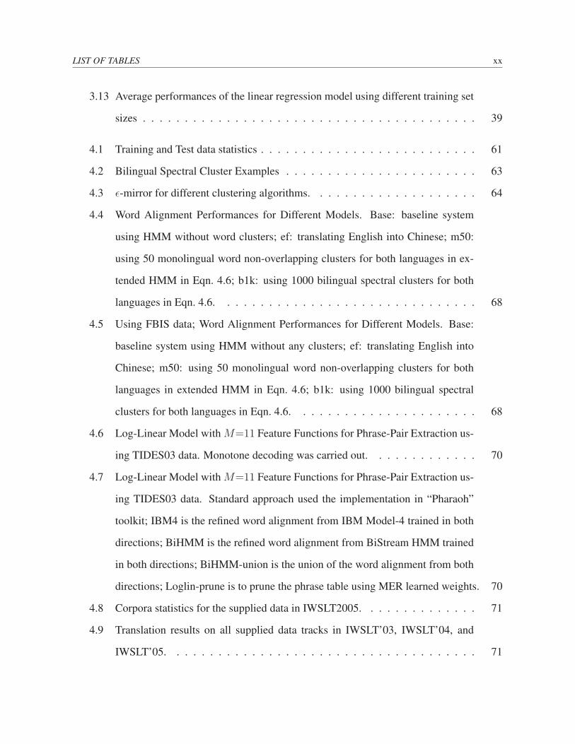
3.13 Average performances of the linear regression model using different training set
sizes . . . . . . . . . . . . . . . . . . . . . . . . . . . . . . . . . . . . . . . . 39
4.1 Training and Test data statistics . . . . . . . . . . . . . . . . . . . . . . . . . . 61
4.2 Bilingual Spectral Cluster Examples . . . . . . . . . . . . . . . . . . . . . . . 63
4.3 ε-mirror for different clustering algorithms. . . . . . . . . . . . . . . . . . . . 64
4.4 Word Alignment Performances for Different Models. Base: baseline system
using HMM without word clusters; ef: translating English into Chinese; m50:
using 50 monolingual word non-overlapping clusters for both languages in ex-
tended HMM in Eqn. 4.6; b1k: using 1000 bilingual spectral clusters for both
languages in Eqn. 4.6. . . . . . . . . . . . . . . . . . . . . . . . . . . . . . . 68
4.5 Using FBIS data; Word Alignment Performances for Different Models. Base:
baseline system using HMM without any clusters; ef: translating English into
Chinese; m50: using 50 monolingual word non-overlapping clusters for both
languages in extended HMM in Eqn. 4.6; b1k: using 1000 bilingual spectral
clusters for both languages in Eqn. 4.6. . . . . . . . . . . . . . . . . . . . . . 68
4.6 Log-Linear Model with M=11 Feature Functions for Phrase-Pair Extraction us-
ing TIDES03 data. Monotone decoding was carried out. . . . . . . . . . . . . 70
4.7 Log-Linear Model with M=11 Feature Functions for Phrase-Pair Extraction us-
ing TIDES03 data. Standard approach used the implementation in “Pharaoh”
toolkit; IBM4 is the refined word alignment from IBM Model-4 trained in both
directions; BiHMM is the refined word alignment from BiStream HMM trained
in both directions; BiHMM-union is the union of the word alignment from both
directions; Loglin-prune is to prune the phrase table using MER learned weights. 70
4.8 Corpora statistics for the supplied data in IWSLT2005. . . . . . . . . . . . . . 71
4.9 Translation results on all supplied data tracks in IWSLT’03, IWSLT’04, and
IWSLT’05. . . . . . . . . . . . . . . . . . . . . . . . . . . . . . . . . . . . . 71
LIST OF TABLES xxi
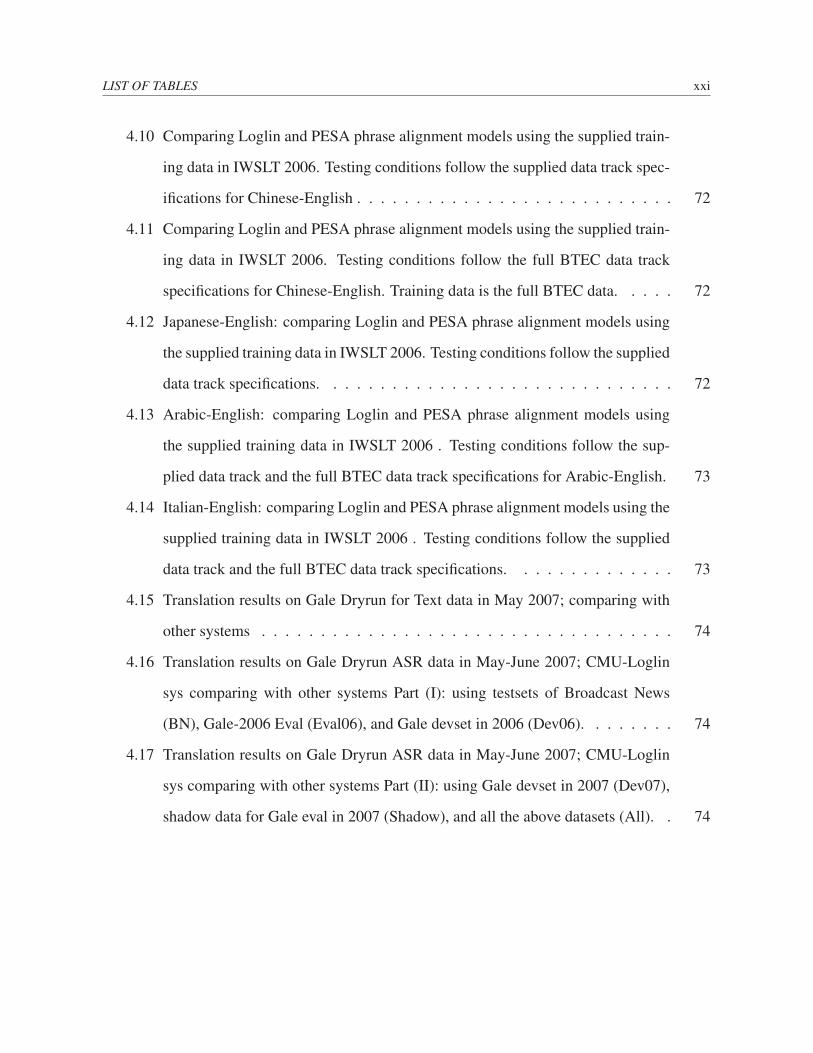
4.10 Comparing Loglin and PESA phrase alignment models using the supplied train-
ing data in IWSLT 2006. Testing conditions follow the supplied data track spec-
ifications for Chinese-English . . . . . . . . . . . . . . . . . . . . . . . . . . . 72
4.11 Comparing Loglin and PESA phrase alignment models using the supplied train-
ing data in IWSLT 2006. Testing conditions follow the full BTEC data track
specifications for Chinese-English. Training data is the full BTEC data. . . . . 72
4.12 Japanese-English: comparing Loglin and PESA phrase alignment models using
the supplied training data in IWSLT 2006. Testing conditions follow the supplied
data track specifications. . . . . . . . . . . . . . . . . . . . . . . . . . . . . . 72
4.13 Arabic-English: comparing Loglin and PESA phrase alignment models using
the supplied training data in IWSLT 2006 . Testing conditions follow the sup-
plied data track and the full BTEC data track specifications for Arabic-English. 73
4.14 Italian-English: comparing Loglin and PESA phrase alignment models using the
supplied training data in IWSLT 2006 . Testing conditions follow the supplied
data track and the full BTEC data track specifications. . . . . . . . . . . . . . 73
4.15 Translation results on Gale Dryrun for Text data in May 2007; comparing with
other systems . . . . . . . . . . . . . . . . . . . . . . . . . . . . . . . . . . . 74
4.16 Translation results on Gale Dryrun ASR data in May-June 2007; CMU-Loglin
sys comparing with other systems Part (I): using testsets of Broadcast News
(BN), Gale-2006 Eval (Eval06), and Gale devset in 2006 (Dev06). . . . . . . . 74
4.17 Translation results on Gale Dryrun ASR data in May-June 2007; CMU-Loglin
sys comparing with other systems Part (II): using Gale devset in 2007 (Dev07),
shadow data for Gale eval in 2007 (Shadow), and all the above datasets (All). . 74
LIST OF TABLES xxii
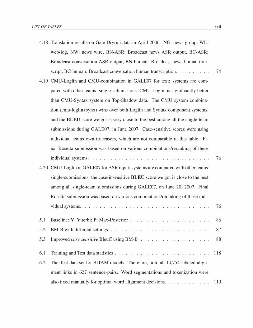
4.18 Translation results on Gale Dryrun data in April 2006. NG: news group, WL:
web-log, NW: news wire, BN-ASR: Broadcast news ASR output, BC-ASR:
Broadcast conversation ASR output, BN-human: Broadcast news human tran-
script, BC-human: Broadcast conversation human transcription. . . . . . . . . 74
4.19 CMU-Loglin and CMU-combination in GALE07 for text; systems are com-
pared with other teams’ single-submissions. CMU-Loglin is significantly better
than CMU-Syntax system on Top-Shadow data. The CMU system combina-
tion (cmu-loglin+synx) wins over both Loglin and Syntax component systems,
and the BLEU score we got is very close to the best among all the single-team
submissions during GALE07, in June 2007. Case-sensitive scores were using
individual teams own truecasers, which are not comparable in this table. Fi-
nal Rosetta submission was based on various combinations/reranking of these
individual systems. . . . . . . . . . . . . . . . . . . . . . . . . . . . . . . . . 76
4.20 CMU-Loglin in GALE07 for ASR input; systems are compared with other teams’
single-submissions. the case-insensitive BLEU score we got is close to the best
among all single-team submissions during GALE07, on June 20, 2007. Final
Rosetta submission was based on various combinations/reranking of these indi-
vidual systems. . . . . . . . . . . . . . . . . . . . . . . . . . . . . . . . . . . 76
5.1 Baseline: V: Viterbi; P: Max-Posterior . . . . . . . . . . . . . . . . . . . . . . 86
5.2 BM-B with different settings . . . . . . . . . . . . . . . . . . . . . . . . . . . 87
5.3 Improved case sensitive BleuC using BM-B . . . . . . . . . . . . . . . . . . . 88
6.1 Training and Test data statistics . . . . . . . . . . . . . . . . . . . . . . . . . . 118
6.2 The Test data set for BiTAM models. There are, in total, 14,754 labeled align-
ment links in 627 sentence-pairs. Word segmentations and tokenization were
also fixed manually for optimal word alignment decisions. . . . . . . . . . . . 119
LIST OF TABLES xxiii
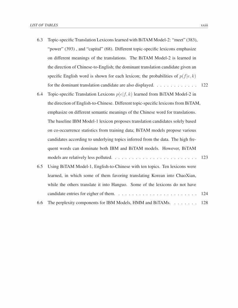
6.3 Topic-specific Translation Lexicons learned with BiTAM Model-2: “meet” (383),
“power” (393) , and “capital” (68). Different topic-specific lexicons emphasize
on different meanings of the translations. The BiTAM Model-2 is learned in
the direction of Chinese-to-English; the dominant translation candidate given an
specific English word is shown for each lexicon; the probabilities of p(f |e, k)
for the dominant translation candidate are also displayed. . . . . . . . . . . . . 122
6.4 Topic-specific Translation Lexicons p(e|f, k) learned from BiTAM Model-2 in
the direction of English-to-Chinese. Different topic-specific lexicons from BiTAM,
emphasize on different semantic meanings of the Chinese word for translations.
The baseline IBM Model-1 lexicon proposes translation candidates solely based
on co-occurrence statistics from training data; BiTAM models propose various
candidates according to underlying topics inferred from the data. The high fre-
quent words can dominate both IBM and BiTAM models. However, BiTAM
models are relatively less polluted. . . . . . . . . . . . . . . . . . . . . . . . . 123
6.5 Using BiTAM Model-1, English-to-Chinese with ten topics. Ten lexicons were
learned, in which some of them favoring translating Korean into ChaoXian,
while the others translate it into Hanguo. Some of the lexicons do not have
candidate entries for eigher of them. . . . . . . . . . . . . . . . . . . . . . . . 124
6.6 The perplexity components for IBM Models, HMM and BiTAMs. . . . . . . . 128
LIST OF TABLES xxiv
6.7 Improved perplexity for training data for Chinese words with different number of
Chinese characters – each corresponds to two bytes. IBM Model-1 is the base-
line for BiTAM Model-1, which is learned using ten topics. The word-length
is measured as number of Chinese characters. The ascii characters, and the
punctuation marks are not considered as Chinese words, and are not listed in the
above table. However, they are considered in the computation of the perplexity
for the whole corpus “All”, as shown in the bottom of the table. Because the
singer-byte character corresponds to high-frequent punctuations with very low
perplexity, the overall perplexity (‘All’) is still small in terms of perplexity. . . . 129
6.8 Measuring Translation Lexicons’ Size, Distribution shape, and Sharpness for
IBM Model-1, HMM, IBM Model-4 and BiTAM models. . . . . . . . . . . . . 133
6.9 Evaluating Word Alignment Accuracies and Machine Translation Qualities for
BiTAM Models, IBM Models, and HMMs using the Treebank data in Table 6.1.
A trigram LM was trained using 180 million words (selected from Giga words
corpus) for decoding. . . . . . . . . . . . . . . . . . . . . . . . . . . . . . . . 134
6.10 Evaluating Word Alignment Accuracies and Machine Translation Qualities for
BiTAM Models, IBM Models, HMMs, and boosted BiTAM Model-3 using all
the training data listed in Table. 6.1. . . . . . . . . . . . . . . . . . . . . . . . 136
6.11 Word Alignment Accuracy (F-measure) for HM-BiTAM Model-1, comparing
with IBM Models, and HMMs with a training scheme of 18h743 on the Treebank
data listed in Table 6.1. HM-BiTAM-A only updates the topic-specific lexicons;
HM-BiTAM-B updates both lexicons and the jump-table; HM-BiTAM-C extend
the HMM network with special treatment of NULL word as in Section 6.4.4. . 137
LIST OF TABLES xxv
6.12 Log-Likelihood and averaged perplexities for unseen documents. Sources were
paired with reference. The documents covered genres of news, speech, and edi-
torial from seven news agencies. BiTAM models are then applied to infer topic
assignments for the documents. The conditional likelihood P (F |E) for each
document are computed via the variational E-step of the proposed BiTAM models.140
6.13 Non-symmetric Dirichlet Priors learned for HM-BiTAM Model-2 . . . . . . . 141
6.14 Decoding MT04 10-documents: Gale systems’ output from CMU, IBM and
UMD, as of May 09, 2007. . . . . . . . . . . . . . . . . . . . . . . . . . . . . 143
6.15 Decoding MT04 10-documents: Gale systems’ output from CMU; Experiments
using the topic assignments inferred from oracle document-pairs: testing mono-
lingual document paired with its English translations. case-insensitive BLEU
score (BLEUr4), NIST score, and case-sensitive BLEU score (BLEUr4c) are
reported. . . . . . . . . . . . . . . . . . . . . . . . . . . . . . . . . . . . . . . 146
6.16 The p-values for one-tailed paired t-test . . . . . . . . . . . . . . . . . . . . . 147
Chapter 1
Introduction
1.1 Machine Translation
In this thesis, we view machine translation, in essence, as a process to abstract the meaning of
a text from its original forms and reproduce the exact meaning with different forms in a second
language. In this process, what are supposed to change are the form and the code only, and what
should remain intact and unchanged are the meaning and the message. The goal of this thesis
is to empower statistical alignment models with the abilities of “learning to translate”, from
shared evidences at different levels of translational equivalences — covering from the direct
observations of word-pairs to the hidden bilingual concepts.
It has been one of the most formidable tasks to fulfill in natural language processing since
1947, when the concept of machine translation first emerged, and was initially documented in
Weaver (1949). For end-users, machine translation means automatically translating texts from a
source language (e.g., Chinese) into texts in a target language (e.g., English). We, therefore, use
these end-user source and target terminologies throughout this thesis.
1
1.2. Towards an Ideal of Translation 2
1.2 Towards an Ideal of Translation
The recent success of Statistical Machine Translation (SMT) seen in the last decade emphasizes
data-driven approaches. These approaches learn from the statistics on the translation patterns
extracted from parallel corpora — each data point is a source sentence together with its transla-
tion in the target language. Data-driven SMT requires sufficient, relevant and representative data,
which is challenging to collect. For high-density language-pairs (e.g., Chinese-English), the par-
allel data seems to be large: in the range of hundreds of millions of words in the TIDES project.
However, compared with the available size of monolingual data (e.g. 200 billion English words)
for training a trigram language model, the amount of parallel data is relatively even smaller for
translation models with parameters in bilingual space. Secondly, current machine translation
models are still relatively knowledge-poor with respect to monolingual linguistic analysis: they
rely only on bag-of-word representations and the associated word correspondences and align-
ments. For instance, models such as IBM’s (Brown et al., 1993) rely on word mixture models,
which more or less act as bottlenecks to capture the rich variations and hidden factors in trans-
lation processes. Faced with many challenges including insufficient parallel data, non-flexible
and less expressive translation models, machine translation (MT) still has not lived up to our
expectations.
When comparing with human translators, we get even more key clues why the current state-
of-the-art machine translation output does not yet reach the level of human translations, and
potentially improve state-of-the-art translation systems. A professional human translator is usu-
ally a master of both languages, equipped with necessary knowledge of the social and cultural
facts, and is very familiar with the domain specific facts. In a detailed study in chapt.11 of (Nida,
1964) “Toward a Science of Translating”, the professional translators’ behaviors are divided into
a few detailed steps, ranging from inferring topics from document level context to revising hy-
potheses iteratively. To be more specific, the professional translators’ behaviors can be divided
into nine steps or three rounds. The first round involves reading the entire document and ob-
1.3. The Organization of This Thesis 3
taining background information; The second round involves comparing existing translations and
generating initial sufficiently comprehensible translations; The third round involves revising the
translations from aspects including styles and rhythms, reactions of receptors, and the scrutiny of
other competent translators. Even though some of the steps listed above are optional, several key
aspects are missing in the current state-of-the-art translation systems especially the document-
level concepts acquisition in the first round.
An ideal machine translation system should be able to leverage a large amount of data re-
sources and multiple information streams from monolingual or bilingual analysis in statistical
or linguistic forms, and be able to self-adapt the model parameters given feedbacks from hu-
man editors or in-domain data. In this thesis, we investigate three aspects to improve the system:
sentence-pair alignment for mining parallel data, improving word-pair and phrase-pair alignment
models, and introducing hidden concepts to generalize over current translation models.
1.3 The Organization of This Thesis
To approximate the ideals, a general framework for building a SMT system is outlined in this
thesis: it starts from mining parallel corpora; bilingual phrase-pairs as hidden structures are
embedded to capture context beyond bag-of-word representations; hidden bilingual concepts
are inferred and fused to enrich the model’s dependency structure and expressive power; the
proposed models have tractable optimizations and inference.
Overall, translational equivalences are modeled from not only the observations of sentence-
pairs, phrase-pairs (block), and word-pair, but also the hidden bilingual concepts. In this thesis,
generative models are mainly used for modeling the translation equivalences, because transla-
tion itself involves a lot of hidden factors, and generative models are modular, scalable to large
training data and easier to be combined with other models. Specific expected contributions of
this thesis include the following:
• Modeling translation at document and sentence levels. This is to design a parallel document
1.3. The Organization of This Thesis 4
and sentences aligner to automatically collect bilingual parallel data, from web sources, to
provide more data for training translation models. This includes a model for bilingual
comparable document-pairs, a parallel sentence-pair aligner, and an efficient optimization
component to combine multiple features at different translational equivalence levels for
selecting high quality bilingual sentence-pairs;
• Modeling translations at the phrase and word levels. Two main aspects are explored: mod-
eling multiple information streams and modeling hidden blocks. The multiple information
streams are to enhance the expressive power of state-of-the-art translation models (esp.
HMM) and improve the dependency structure of such models. The hidden blocks (phrase-
pairs) are very good features for localizing word alignments decisions.
• Leveraging graphical model representations for designing new translation models. The
structure of the graphical models (qualitative aspect) defines the dependency between the
nodes and edges; the potentials over the edges and cliques exemplifies the quantitative
aspect. The hidden concept translation models (BiTAMs) can be viewed as hierarchical
models with each topic corresponding to a point on the conditional word-simplex, with
each English word invoking a simplex.
The work in this thesis will provide not only an initial solution toward breaking the bottle-
necks of machine translation, but also pave the path to a more theoretically sound framework
via graphical model language to reformulate problems of machine translation, and potentially
related alignment problems of annotated data.
The models proposed in this thesis were mainly tested for the language-pair of Chinese-
English in both small-scale systems and large ones such as GALE systems. Other language-pairs
such as Japanese-English, Arabic-English and Italian English were also tested under the IWSLT
evaluation conditions in travel domain.
Chapter 2
Literature Review
Potentially inspired by the successes of noisy channel model in speech recognition, practically,
most of the statistical machine translation approaches have some corresponding counterparts in
speech recognition. There are many methodologies in speech recognition, which maybe help-
ful in current statistical machine translation, as summarized in Och and Ney (2001). Another
evidence is that most of the statistical systems can be formulated as the weighted finite state
transducers (WFST), e.g. the system of Shankar and Byrne (2003). Descriptions of the statisti-
cal alignment models such as HMM and IBM models will be explained in detail and extended
through the following chapters in this thesis.
The work in this thesis focuses on statistical phrase-based machine translation approaches;
the other approaches such as interlingua, transfer-based, example-based, syntax-based may po-
tentially benefit from the facts and results investigated in this thesis. The approaches can usually
be described in a so-called machine translation pyramid: “Vauquois pyramid”(Vauquois, 1968)
(also called Vanquois triangle) as in Figure 2.2. Different approaches go to different levels of
this pyramid, and utilize different representations of the semantics and syntax in one or both of
the languages for machine translation.
Throughout the thesis, the notations in Brown et al. (1993) are followed; additional notations
5
6
are used in necessary to explain the proposed algorithms. The fundamental model for statistical
machine translation is the noisy channel model in Eqn. 2.1:
e = arg maxe
Pr(e)Pr(f |e), (2.1)
where e is an English word, e is the English sentence; I is the length of e; E is the English
vocabulary; E is the English document; ei is the English word at the position of i in e indexed
by i; fj is a French word at position j in the French sentence f indexed by j with sentence
length of J . Pr(e) is Language Model, and Pr(f |e) is the Translation Model. Current state-of-
the-art translation models are mostly based on word-level mixture models such as the translation
lexicon Pr(f |e), the fertility models Pr(φ|ei) (φ: number of words), and the distortion models
Pr(j|i, l, m).
The SMT translation models, investigated in this thesis, can be summarized using Figure 2.1.
The upper panel describes the parallel data mining from from comparable corpora. Figure 2.1.a
and Figure 2.1.b describe the noisy channel models in both directions: English-to-Foreign and
Foreign-to-English. Figure 2.1.c described a symmetrizing approach in combining the statis-
tics collected from the two directions. Figure 2.1.d is an undirected model in which the joint
probability is directly modeled instead of conditional probability. Figure 2.1.e is a typical joint
model, in which a hidden concept is explicitly introduced. Figure 2.1.f is a hierarchical model,
where the hidden concept is used as one additional layer of mixtures. In general, we can classify
current phrase-based approaches into the above clusters.
As also discussed in the previous chapter, the current state-of-the-art SMT systems are fac-
ing insufficient training data and the lack of power to capture various translation patterns due to
underlying word-mixture models. The very first approach, explored in this thesis, is to increase
the coverage of the translation patterns by mining parallel data from comparable data. Models
such as a log-linear phrase-pair alignment model, embedding blocks for word-alignment, and
bilingual topic-admixture models were also explored. Chapter 3 focuses on document and sen-
2.1. Approaches to Mining Parallel Data 7
Figure 2.1: An Overview of Translation Models. The upper part is mining parallel data from comparable corporafor training translation models. The lower part contains instances of translation models ranging from noisy channelmodels in (a) and (b), to those with hidden concepts as in (e) and (f).
tence alignment, corresponding to the upper part of Figure 2.1; Chapter 4 and Chapter 5 focus
on extending the baseline models as in Figure 2.1.a and Figure 2.1.b; Chapter 6 focuses on mod-
eling bilingual concepts, corresponding to Figure 2.1.e. In this chapter, approaches to machine
translations, which are relevant to the works in this thesis, are reviewed.
2.1 Approaches to Mining Parallel Data
As a fundamental resource to translation models in Figure 2.1, parallel data is vital not only to
machine translation but also to other multilingual applications such as cross-lingual information
2.1. Approaches to Mining Parallel Data 8
retrieval (Gao and Nie, 2006), which rely on large bilingual knowledge sources. Increasing
coverage of translation patterns and vocabulary will help significantly to reduce uncertainties
and errors in the statistical translation process.
As many news agency covers the same news stories in multiple languages, the newswire doc-
uments usually contain many documents in two or more languages conveying the same meaning
in machine readable form; the documents are translation-alike, but they are not strictly trans-
lations of one another. We refer to such data as the comparable data, and the translation-like
document pairs as comparable document-pairs. The ten years’ collection of Xinhua News cor-
pora (LDC2002E18), in the work described in Chapt. 3, is a case in point.
Mining parallel data from the comparable corpora has been an active and expanding topic
in natural language processing. However, it is not trivial at all. The comparable data is usually
noisy. A sentence can be translated into two sentences; or a sentence or even a paragraph can be
missing from comparable document-pairs. Also, most of the previous works mainly worked on
similar language-pairs, such as French-English, ignoring the difficulties inherited in structurally-
distant language-pairs like Chinese-English or Japanese-English.
Previous approaches range from using simple segment-lengths (Brown and Mercer, 1991) to
computationally intensive approaches using MaxEnt model as in Munteanu and Marcu (2005).
Segment-lengths are highly relevant for translation pairs. Early works assumed simple log
of the ratio of segment-lengths in words (Brown and Mercer, 1991) or characters (Gale and
Church, 1991) as a Gaussian distribution to check translation-like sentence-pairs, assuming that
the length of a translation is not too distorted in the translation processes. Anchor points, such
as paragraph and sentence boundaries, and cognates (Simard and Isabelle, 1992) were shown to
be very necessary to narrow down the alignment decisions (Church, 1993). The simple length
based approach is efficient to compute and is effective for large-scale language-similar compa-
rable corpora, for instance the Indo-European language pairs. However, real texts are not cleanly
marked, and lexical features become necessary to identify if two sentences are translation-like.
2.2. Approaches to Translation Models 9
Because the length-based methods ignored the word-identities, they are not robust to non-
literal translations or language-pairs which are structurally different. In Kueng and Su (2002), it
was shown when the style is different, the length-based approach’s performance can drop from
98% to 85%. In Chen (1993), lexical featues of 1:1 word-pairs were used in a dynamic program-
ming with thresholding. Wu (1994) had tried both length and cognate features on Hong Kong
Hansard English-Chinese corpus, and a 7.9% error rate has been reported. Further evidences
using lexical features were reported in Haruno and Yamazaki (1996). Compared with the statis-
tical approaches, they are quite different in the way they use word-correspondence information
and the parameters in their models. In this thesis work, we are aimed at structurally-different
language pairs: Chinese-English, and the comparable corpora is highly noisy containing many
insertions (0:1), deletions (1:0) and non 1:1 mappings. We designed specific background mod-
els to handle the noise including the insertions and deletions, and we embedded both lexical
features and sentence-length features in a dynamic programming framework to be explained in
Chapt. 3. The results produced in our approaches were also released through LDC under the
catalog number of LDC2002E18.
2.2 Approaches to Translation Models
2.2.1 Generative Models
Generative models simulate the process of generating the observations, given some hidden vari-
ables. It defines the a joint distributions of the observations and the hidden variables, and learning
the parameters for maximizing the data likelihood, typically through Expectation Maximization
or its variants. models. According to the human translation studies in Nida (1964), there are
potentially a few hidden factors influencing the translation process. In this sense, generative
models are well suited for machine translation. Generative models are modular, and can be eas-
ily combined into more complex models. In the later of this thesis, we will see several extensions
to the generative models.
2.2. Approaches to Translation Models 10
Interlingua Semantics
English SemanticsFrench Semantics
French Syntax English Syntax
English WordsFrench Words
Figure 2.2: An Overview of Translation Models: “Vauquois pyramid”
The IBM Models in Brown et al. (1993) are typical generative models, laying down a foun-
dation for statistical machine translation. Showing in Eqn. 2.1 is a noisy-channel model scheme.
The model learns word-translation pairs from parallel corpora through the Expectation Maxi-
mization (EM) algorithms. Shown in Figure (2.1.{a,b}) are general representations of the IBM
Model-1 through Model-5.
These models approximate the translation process as a process of manipulating bilingual
word-pairs: permutations, substitutions, and insertions/deletions with NULL token introduced
into the generative process. To be more specific, the generative story is approximately as follows:
delete or duplicate n times of each English word ei according to a fertility table φ(n|ei); second,
once the desired length of the English sentence is reached, add the necessary number of NULL
words to generate the French words, which have no corresponding English translations; third,
after these operations, try to map the French words with English word in a one-to-one fashion
which is preferred by the noisy-channel model; fourth after all the word pairs are connected,
the resulting French word string is permuted into a possibly different position, as controlled by
a distortion table d(j|i, I, J). These mixture models are mainly located near the paths directly
2.2. Approaches to Translation Models 11
from F to E at the bottom of the Vanquois pyramid in Figure 2.2.
There are several problems in traditional IBM Models due to the simplified generative process
mentioned above. Firstly, these models ignored the context, and only model the word-level
translation equivalences. Secondly, the models are not bijective due to the underlying noisy
channel models applied, and the generative stories are only half of the truth because it pretends
one side of the parallel data is unseen. Thirdly, the models ignored the knowledge from the
monolingual data assuming no correlations or connections of two monolingual words in the
translation space. These assumptions are not sound for modeling the translation process, and it
can be verified easily from the data of professional human translators.
However, generative models, such as IBM models, are modular, and can be easily combined
and composed to form more complicated models. HMM is such a model to generalize over IBM
Model-1: a chained IBM Model-1 with additional alignment dependency. The work of BiTAM
Models in Chapt.6 generalize over both IBM Model-1 and HMMs. Simple additional heuristics
can also be applied to remedy the noisy-channel models. For instance, a typical approach is to get
the intersection word alignment from both directions, and grow the intersection with additional
aligned word-pairs seen in the union. This approach has been widely applied in Koehn (2004b),
Och and Ney (2003), Tillmann (2003). The results from these works indicate that if the model
can symmetrize the parameter estimation by considering statistics collected from both directions,
one may gain further improvements (Zens et al., 2004) and (Liang et al., 2006b). This evidence is
leveraged in the work in Chapt. 5, in which the block-level information is modeled for collecting
the fractional counts from context.
2.2.2 Log-Linear Models
Current state-of-the-art phrase-based statistical machine translation systems combine the sub
generative models in a log-linear framework, and limit the training to be just a few parameters
(typical ten to twenty) in (Och and Ney, 2002). There are several extensions to IBM models.
Most of the log-linear models are targeted at word-alignment tasks, or the decoding process,
2.2. Approaches to Translation Models 12
which combines a few underlying models together in a log-linear framework.
In Liang et al. (2006a), the discriminative training for the decoding parmeters were studied
using data from reachable and non-reachable N-Best list generated from the decoder. In the
log-linear model style for word alignment, the joint probability of English and Foreign words
is estimated, such as the the log-linear models for word alignment (Liu et al., 2005). However,
the performance reported is very close to the results obtained by using heuristics to combine
both directions of the trained IBM models. Further investigations should be carried out. In
Lacoste-Julien et al. (2006), the word alignment is projected as a quadratic programming. In
Fraser and Marcu (2006), the sub-models in IBM Model-4 are combined together using a log-
linear model framework, in which each feature function corresponds to a generative model. The
weights associated with each feature function is then learned in a supervised fashion with small
labeled data set. One key problem for these approaches is the need of optimization for millions
of parameters. The works win by choosing appropriate thresholds from a development data set
in a greedy-style algorithm. Most of the improvements over IBM Model-4 are quite small. On
the other hand, IBM Model-4 does not yet use the same labeled data set as used in the log-linear
model, to guide the learning. Therefore, the improvement from log-linear model is not yet as
significant as expected.
In Papineni et al. (1998), a direct translation model is proposed to view translation as a direct
communication so that the multiple features can be taken into account to help machine transla-
tion. One of such model instances is the work by Ittycheriah and Roukos (2005). They learned a
Maximum Entropy Model from hand-aligned data. Their model is a mixture of supervised and
unsupervised methods, taking advantages of a few feature functions relevant to the alignment
tasks. Their models performed significantly better than the IBM Model-4. In Ittycheriah and
Roukos (2007), the model parameters are reduced significantly but still maintain the the prop-
erty of easy integration of multiple feature streams and optimization. Watanabe et al. (2007)
directly optimized the model parameters under a large margin framework, and reported gain for

2.2. Approaches to Translation Models 13
unseen data is still marginal.
Our work using a log-linear model solely for phrase-alignment, in which each feature func-
tion is a generative model. Each of the sub-model is learned in a unsupervised fashion, and
the combination of them is an exponential model, and the optimization is limited to only a few
parameters. Working for phrase-level alignment provides a easier framework to take a few in-
formative yet overlapping feature functions. More details are in Chapt. 4.
2.2.3 Syntax-based Models
In terms of the motivations, syntax based models have a grammar-channel view of the parallel
data. As shown in Figure (2.1.e), the models range from the simplest one such as Bilingual
Bracketing (Wu, 1997) to more complicated ones including tree-to-tree and tree-to-string models
in Yamada and Knight (2001). The simple bilingual bracketing grammar works well in many
cases of word alignments and as well as word reordering constraints in decoding algorithms.
A → [A,A]
A → <A,A>
A → e/f
A → e/ε
A → ε/f (2.2)
where “<·, ·>” indicates the bracketing along the reverse diagonal, and “[·, ·]” along the diago-
nal; ε indicates that a NULL word is being aligned to. One can train the standard IBM Model-1
lexicon Pr(f |e) to lexicalize the generation rules of A → e/f ; with the dynamic programming,
the word alignment can be traced through an inside-outside style algorithm. Zhao and Vogel
(2003) showed the performance obtained from this approach is better than IBM Model-4. In
Zhang and Gildea (2005), a stochastic lexicalized ITG for alignment is proposed. The ITG is
enhanced by making the orientation choices dependent on the real lexical pairs that are passed
2.2. Approaches to Translation Models 14
up from the bottom. The improvements of alignment accuracy over IBM Model-4 comes at the
expense of a high complexity of O(n8), where n is the sentence length. In Zens and Ney (2003),
ITG was found to be very helpful when combing with the heuristics used in traditional IBM
models.
These approaches proved the simple syntax constraints can improve translation models. How-
ever, more complicated approaches suffer from both data sparseness and expensive computa-
tions, and therefore, are less competitive to the IBM Models (such as IBM Model-4) using large
training data.
Recently, the use of syntax to improve machine translation system has attracted a lot of atten-
tion. Modeling syntax across language pairs, in general, is not easy as the syntax structures for
two languages are usually very different (e.g., SVO in English, SOV in Japanese, VSO in Ara-
bic; S: subject, V: verb, O: object); translators usually do not strictly follow the syntax structure
in the source sentence. However, there is a big room for improvement with regard to better syn-
tax modeling: in evaluations, the target language proficiency is more highly prized than source
language proficiency; the oracle experiments indicate most of the good translation candidates
are well represented in current translation models, but the language model employed is not yet
able to select the best ones. Syntax modeling is one of the key aspects different from speech
recognition using the same noisy-channel paradigm, partially because the word-orders becomes
an essential problem in translation.
Overall, syntactic models have potential benefits of using more complex language models
to better synthesize the translation hypothesis. The reason is that a syntactic translation model
outputs tree structured hypotheses rather than surface strings and the trees can be readily scored
by tree-based language models. This brings the advantage of better models for word reordering
and functional words generations, which, in turn, influence word choices and potentially get
more n-gram translated correctly.
Approaches in this field vary with different success. The earliest work along this line maybe
2.2. Approaches to Translation Models 15
the work in Wu (1997), which showed that restricting word-level alignments between sentence-
pairs to an ITG grammar (binary branching trees) can significantly improve the performance with
a solution of a polynomial-time algorithm. The work in Yamada and Knight (2001) assumes the
source sentence not only contains the words to be translated but also specifies the syntax structure
to be followed in organizing the words into a target sentence (hypothesis). In this sense, it
uses incomplete syntactic information in modeling the syntax transfer: only the target (English)
sentence’s parsing structure is taken into considerations in the modeling (source-string-to-target-
tree). Later, in the work of Charniak et al. (2003), the translation model is combined with a
syntax-based language model. Motivated by the fact that real parallel sentences generally do not
exhibit parse-tree isomorphism, Gildea proposed loosely string-to-tree 1 with a clone-operation
and tree-to-tree with m-to-n mapping of up to two nodes on either side of the tree (Gildea, 2003).
These alignment models provide flexibilities for word alignments not conforming to the original
tree structure. In the studies of Fox (2002), dependencies were found to be more consistent
than constituent structure between French and English. A comparison following the tree-to-tree
models were carried out in Gildea (2004); the constituent-based alignment model is shown to
significantly outperforms the dependency based model on a relatively small data set for Chinese-
English.
In Melamed (2004), generalized parsers are proposed for machine translation by extending
common notions of parsing: the logics of input and output, a multitext grammar, a semiring
structure and an inference or search strategy. Evaluations of the proposed approach, however, is
not yet presented in detail.
In Och et al. (2004), a log linear model integrated a number of syntax features including
the works mentioned above. Surprisingly, the features from IBM Model-1 are shown to be
the most informative feature in this log-linear model to re-rank the N-Best list from a state-
of-the-art machine translation system. These experiments show the discriminative training is1Note we are using End-User terminologies for source and target

2.2. Approaches to Translation Models 16
not powerful enough facing many parameters; or the re-ranking of the N-Best list may not be a
good framework for testing the syntax features; or the syntax features inferred from the available
toolkits may contain too much noise. Potentially, the improvements may not be well captured or
represented by BLEU scores. The overall results indicate current models are still far away from
tightly integrating the syntax features.
The work in Chiang (2005) successfully generalized the phrase alignments by introducing
variables in the phrase-pairs, and decode unseen sentence by CKY style parsing. Other ap-
proaches, such as Galley et al. (2006), also generalize syntax rules from the underlying word-
alignment and phrase-alignment. In Graehl and Knight (2004), algorithms to learn the tree-to-
tree mapping rules are described. In Hwa et al. (2002), the human translations from Chinese
to English preserved only 29−42% of the unlabeled Chinese dependencies. Smith and Eisner
(2006) showed that relaxing synchronous process of generating trees can fit better to the bilin-
gual data, and the word alignment performances match standard baselines by allowing greater
syntactic divergence. More or less, the assumption is human translators might be translating
with information “inspired by the source sentence”; the syntactic constituents may not be well
kept during this translation process. In Turian et al. (2006), the trees were broken into atoms,
and each atom is one feature in an exponential model, which is learnt via discriminative training.
Because the approaches in this thesis are not aimed at modeling the syntax per se, the chapters
will not follow up with more details unless they are relevant. However, the generative models
in this thesis can be combined with the syntax features in a log-linear model framework as was
done in Och et al. (2004).
2.2.4 Other Models
Other approaches include example-based machine translation (EBMT or memory-based)1, in
general, relies on the alignment of the bilingual texts. It decomposes the unseen source sen-
tences into units, and try to match the source units with those seen in the training corpus. The1Other names are like analogy-based, memory-based, case-based, experience-guided etc.

2.3. Datasets and Evaluations 17
target sentences (or hypothesis) are then generalized from the selected matching units with the
various knowledge of the target language. There are a variety of methods and techniques, which
differ in many levels in these basic processing steps. Overall the underlying message is that the
translation process often involves the finding or recalling of analogous examples, the discovery
or recollection of how a particular expression or some similar phrase has been translated before.
A detailed review can be found in Somers (1999). Hutchins (2005) and Carl and Way (2003)
have more detailed disccusions between EBMT and SMT.
2.3 Datasets and Evaluations
Training data (parallel datasets) for machine translation is always limited for most of the lan-
guage pairs in the world. The parallel datasets are mainly from LDC(Linguistic Data Consor-
tium) for the TIDES 1 and GALE 2 projects. There is also domain specific data sets used in the
speech-to-speech translation in traveling domain such as BTEC: Basic Travel Expression Cor-
pus(Takezawa et al., 1999), which is a multilingual speech corpus containing tourism-related
sentences similar to those found in phrase books.
The focus in this thesis work is mainly Chinese-English translation. The evaluation tracks in
the TIDES project from 2001 to 2005 include large-data-tracks for both language pairs and one
small-data-track for Chinese-English. The small data track (LDC2003E07) evaluation is very
close to the scenarios for translating language pairs with scarce resources (low-density language
pairs), while the large data sets are very close to the scenarios of high-density language pairs for
which the data resources are abundant. For low-density language pairs, the model’s strength is
emphasized, and for high-density language pairs, the model’s efficiency is emphasized. In this
thesis, the domain-specific data sets from BTEC used in speech-to-speech translation in travel
domain will also be evaluated for domain specific translation scenarios. BLEU scores (Papineni
et al., 2002), as shown in Eqn. 2.3, are selected as the main evaluation measure in this thesis to1see http://www.ldc.upenn.edu/Projects/TIDES/index.html2see http://www.ldc.upenn.edu/Projects/GALE/index.html
2.3. Datasets and Evaluations 18
evaluate the translation qualities.
BLEU = BP× exp( N∑
n=1
wn × log(pn)), (2.3)
where BP is the brevity penalty for the translations which are shorted than the reference: BP =
exp(1 − c/r). c is the candidate length in words, and r is the length in words of the reference.
When c > r, there is no brief penalty. pn is the ngram precision for the translation comparing
against the references. Note that, with different versions of the choosing the references’ length
when multiple references are available, there are different versions of the BLEU scores. In this
thesis, we use the original IBM implementation of the BLEU score for evaluating the proposed
models.
Other automatic translation scores and human judgement scores were reported occasionally.
For every controlled experiments, BLEU scores will be reported.
Chapter 3
Mining Translational Equivalences
As introduced previously, one of the bottlenecks of most of the translation systems is insufficient
bilingual data. Data sparseness is always a problem of statistical machine translation. Given
enough translation patterns covered by training data, even a simple model can perform very well.
It is indeed one of the most effective ways to improve systems’ performances by adding more
bilingual parallel data. A case in point is the parallel data from FBIS (Foreign Broadcast Infor-
mation Service, LDC: LDC2003E14), which significantly improved our system’s performance.
Lacking enough training data is a serious problem, especially for low-density language-pairs
such as Hindi-English — the surprising language in the translation exercise by DARPA in the
2003.
3.1 Language Pairs and Resources
From a recent study of the language resources at LDC, there are around 6,900 languages in the
world. Among them, there are about 340 languages which have more than one million speakers
1. Most of these languages have written systems and also web presence, which provides an good
opportunity of mining relevant data for machine translation. The bilingual texts for current trans-
lation systems are still scarce even for the high density language-pairs such as French-English1the numbers are from Max’s presentations at ACL SMT workshop in 2005.
19
3.1. Language Pairs and Resources 20
(350+ million words), Chinese-English (220+ M) and Arabic-English (100+ M) 1. Compared
with the sizes of the monolingual corpora, these numbers seem to be small, but the parameters
for translation models are relatively large. Data collection has also been one of the major tasks
in the TIDES evaluations. The “surprise-language” dry-run in March 2003 emphasized more on
parallel data mining. Sufficient bilingual data resources enable approaches to deeply investigate
current models’ strengths and inspire new models to be explored more effectively. With the fast
growing resources on the web, the need to collect bilingual data from web resources is becoming
more and more important.
In this chapter, models are proposed for aligning bilingual document-pairs and aligning bilin-
gual sentence-pairs from multilingual document pairs published by the major news agencies
around the world. Models for them are usually designed differently, but they can be combined
into one single hierarchical structure detailing with titles, paragraph structures, sentence orders
and other document structures within the full text news story. Different levels of features can be
defined over these identities such as cognates and dictionaries (Simard and Isabelle, 1992).
Monolingual
GigaWord
Corpora
Xinhua News
Sinorama FBIS
EPPS
difficult easy
Figure 3.1: An overview of aligning document- and sentence-pairs from comparable data. The left one representingthe non-parallel monolingual data; the middle one represents the comparable data; the right one represents veryclean parallel documents. From left to right, the tasks become relatively easier.
Figure 3.1 summarizes the general tasks of mining the parallel documents and sentences
ranging from non-parallel and comparable data to very clean parallel data. The GigaWord cor-
pora of English, Chinese and Arabic are all monolingual newswire text collected by LDC. It is
not guaranteed that there are any good document or sentence pairs to mine from these corpora.1the number is a rough estimation on the source language only as in the year of 2006
3.2. Full-text Bilingual Document Alignment Models 21
However, there could be many named entities and other translational equivalence contained in
these corpora. Xinhua News Agency, the largest news agency in mainland China, publishes hun-
dreds of news stories on the web every day in both Chinese and English. The Xinhua news data
collected from the web is usually noisy with a lot of non-parallel segments; but they also contain
very good translation pairs. On the other hand, the FBIS (Foreign Broadcast Information Ser-
vice) corpora are very clean parallel datasets. All the documents are translated by professional
translators. In these datasets, the tasks to mine document pairs and sentences are relatively easy.
3.2 Full-text Bilingual Document Alignment Models
The most typical newswire item is the news story, a coherent self-contained report on a particular
topic or event. Bilingual newswire corpora released by major international news agencies are
mainly in this category; a typical such chunk-based news service generates about 15 ∼ 20MB
per month of raw text. The major Chinese-English bilingual news services include Xinhua News
Agency, Sinorama, BBC, VOA, etc..
The newswire documents collected by LDC have a clear grouping of contents and structures.
For example, the document from Xinhua News Agency usually has a title, followed by the agency
name, dates, reporters’ name and an initial headline of the news story. Parallel documents share
strong similarities in these aspects together with nearly identical paragraph-structure and simi-
lar sentence-orders. To mine parallel documents, the most important features are tokens in the
documents, and the features of the structures including the title, date and reporters names; doc-
ument lengthes are also important in extracting document-level translational equivalences from
the noisy comparable corpora released by news agencies. The data targeted, in this chapter, is
a collection of the comparable documents. These documents were downloaded from the web
sites, tokenized and cleaned. The documents have time-stamp associated with them, specifying
when the documents were published and released. The time information can be used to restrict
the span for seeking parallel documents to improve the speed of the parallel documents mining.
3.2. Full-text Bilingual Document Alignment Models 22
In this thesis, several features are integrated for extracting parallel documents and parallel
sentences through full-text story alignment models (Zhao and Vogel, 2002b) and sentence align-
ment models (Zhao and Vogel, 2002a). Usually the story alignment models are like known-item
retrieval problem assuming that each document has none or only one parallel story in the other
language. The documents are indexed and pseudo queries are designed to retrieve them fol-
lowing typical information retrieval framework. The details will be explained in the following
sections.
3.2.1 Pseudo-Query Models via Standard IR
Let’s start from mining the English parallel documents for given Chinese documents (one can
do the other direction as explained later in this thesis). One approach of creating pseudo query
from a given Chinese document is to use a lexicon or dictionary to translate every Chinese
word into a candidate list of English words. Then all the candidates are merged into a bag-of-
word representation with necessary preprocessing. A query then is created to mine the relevant
English documents using available typical information retrieval schemes. The mined documents
are supposed to be the potential translations of a given Chinese document.
Formulation
In our approach, for each Chinese word wc in a Chinese news story: wjc , j = 1, · · · ,m, the
top three translation words w1e , w
2e , w
3e of wc from our translation model were chosen, and the
union of all the translated English words for one document was collected; stop words were
removed and a pseudo-query was generated. Now the story alignment reduces to the evaluation
of the pseudo-query and the retrieval of one particular document, which is the potential parallel
English story (none or only one parallel story). This is a typical known-item retrieval task stated
in Kanto and Voorhees (1996), where we know there is only one correct answer for a query. We
are interested in retrieving that one particular document instead of retrieving/ranking the entire
set of documents that pertain to a particular subject like in standard IR.
3.2. Full-text Bilingual Document Alignment Models 23
Retrieval Methods
Three standard query methods were investigated: TFIDF, Okapi and LM-JM (Jelinek-Mercer
smoothing). The first two methods differ in term of weighting schemes. Okapi has the advantage
of the term frequency normalization using document length:
TFIDF : tw = log(tf) + 1
Okapi : tw = tf/(tf + 0.5 + 1.5 · doclen/avg(doclen)) (3.1)
Now the pseudo query q and document d are represented by term-weight vectors, of which
the element is an index term’s weightings tw in q and d, defined in Eqn. 3.1. The similarity of q
and d is the inner product of the two vectors.
The third method of LM-JM is a language modeling approach to information retrieval. It
infers a language model for each document and estimates the generation of the query according
to each of the document language models. Then it ranks the documents using those probabili-
ties. In this paper, the document language model (LM) is built as a unigram and the smoothing
method is Jelinek-Mercer (JM), which is fixed coefficient linear interpolation. These standard
information retrieval approaches were implemented in Lemur toolkit 1.
3.2.2 Full-Text Alignment Model-A
Instead of using the pseudo queries as in section 3.2.1, we can directly model the probability that
an English story (Document) DE was the relevant document given a Chinese story (Query) QC :
P (DE|QC). Assume a story is a bag of tokens, then we have:
DE = wie, i = 1, · · · , l
QC = wic, i = 1, · · · ,m (3.2)
The goal is to retrieve relevant English documents DE , which are possible translation candi-1see http://www-2.cs.cmu.edu/ lemur/
3.2. Full-text Bilingual Document Alignment Models 24
dates for the given Chinese document as the pseudo queries QC . The relevance P (DE|QC) is
computed as follows:
P (DE|QC) =∏
we∈DE
∑wc∈QC
P (we, wc|QC) (3.3)
=∏
we∈DE
∑wc∈QC
[P (we|wc, QC) · P (wc|QC)]
'∏
we∈DE
∑wc∈QC
[P (we|wc) · P (wc|QC)],
where we is a word in DE , wc is a word in QC ; P (we|wc) is the translation lexicon, for example
IBM Model-1; P (wc|QC) is a bag-of-word unigram language model. P (wc|QC) could also be
the tf.idf model for each word in the document or other informative term-weighting models as
shown later in the experiment section.
In this model, the words wc in the source language of Chinese will be weighted by the doc-
ument specific language model p(wc|QC), and the repeated occurring content words will have
higher frequency in this query model, and the translations of them, according to a word-to-word
translation lexicon, will also have larger weight in the final decisions for selecting the English
documents as the relevant translation candidates. With suitable weighting schemes, like standard
tf.idf , content words usually have larger weights, and in such, they play more effective role in
determining the translation candidates for a given Chinese document.
Thus, the relevance of an English news story to the given Chinese news story (which is a
query) is directly modeled. For each Chinese news story, we can obtain a ranked candidates list
with a score of relevance attached to each of the candidates. The translation probability acts as a
bridge between the language pairs in an efficient way. It re-weighs each possible English word’s
relevance to the given Chinese story.
The model of P (we|wc) can be learned directly from parallel data, and the P (wc|QC) is
simply a frequency table for a bag-of-word representation of the document. The combination of
the two sub-models is a overall a generative model for mining Chinese-English document-pairs
3.2. Full-text Bilingual Document Alignment Models 25
from comparable data collections.
3.2.3 Full-Text Alignment Model-B
As specified earlier, the other direction for mining the relevant Chinese document-level transla-
tions for a given English document is modeled as follows:
P (QC |DE) =∏
wc∈QC
∑we∈DE
P (we, wc|DE) (3.4)
=∏
wc∈QC
∑we∈DE
[P (wc|we, DE) · P (we|QE)]
'∏
wc∈QC
∑we∈DE
[P (wc|we) · P (we|DE)],
where the lexicon P (wc|we) is learnt from the parallel data. P (we|DE) is a unigram language
model. This model is different from Model-A in that it models relevance directly.
Both the models are aimed at retrieving the parallel document-pairs from the comparable
document-pairs. It is important to have efficient representations and models for this task due
to the large amount of data to work with. The model is aimed at getting initial compara-
ble document-pairs from very noisy comparable document-pairs and the detailed alignments
at sentence-level and word-level can be carried out later with slightly higher computational cost.
3.2.4 Refined Full-Text Alignment Models
Sliding Window
Both the two alignment models in sections 3.2.2 and section 3.2.3 have one common problem:
ignoring the position of the words appearing in the documents (stories). All the documents are
deemed as a bag of words. We know that potential parallel stories have a good portion of
parallel sentences, and token pairs in these sentences usually appear in similar positions of the
corresponding stories. For example, if a token wc is too far away from the position of token we,
it is unlikely for them to form a translation token pair.
While it is hard to model the position of translation pairs, we can approximate the effect by
3.2. Full-text Bilingual Document Alignment Models 26
using a window to constraint the probabilities of translation for the token pair. The refinement
uses alignment Model-B for demonstrating this formalization, which is actually the same for
Model-A. First, we reformulate the documents as tokens with positions:
DE = (we, i), i = 1, · · · , l
QC = (wc, j), j = 1, · · · ,m. (3.5)
Now, the refinement of alignment Model-B is an approximation as follows:
P (QC |DE) =∏
(wc,j)∈QC
[ ∑
(we,i)∈DE
P ((wc, j), (we, i)|DE)]
'∏
wc∈QC
[ ∑we∈DE
P ((wc, j)|(we, i) · P ((we, i)|DE))]
'∏
wc∈QC
[ ∑we∈DE
P (wc|we)P (j|i) · P (we|DE)]
'∏
wc∈QC
[ ∑we∈DE
P (wc|we)P (|j − i|) · P (we|DE)], (3.6)
where P (|j − i|) is the probability of the position difference between the translation token pair
(wc, we). Due to the noise in the data collected from web, it is hard to estimate the probability
accurately. In our approach, a uniform probability within a certain size of window was used as
the following:
p(|i− j|) =
12N
if |i− j| < N
0.0, else, (3.7)
where N is the window size.
The TF.IDF approximation to P (we|DE)
Another refinement is the P (we|DE), which is so far a unigram document language model:
P (we|DE) =c(we; DE)
|DE| =tfwe
|DE| , (3.8)

3.2. Full-text Bilingual Document Alignment Models 27
where tfwe is the term-frequency for the word we in the document DE , and |DE| is the document
length in words. In fact, one can increase the discrimination power by replacing the document
length |DE| with the document-frequency within the whole collection of monolingual English
documents, similar to the tf.idf term-weights for the pseudo query models. Thus, the alignment
model-B P (QC |DE) can be approximated as below:
P (QC |DE) '∏
wc∈QC
[ ∑we∈DE
P (wc|we)P (|j − i|) · (1 + log(tfwe))(log(M)/dfwe)
λ
], (3.9)
where M is the number of English documents in the whole collection, and λ is a normalization
constant. The tf.idf scheme, as used in the pseudo query models, measures the words’ informa-
tive power by computing the statistics from whole corpus collection. This turns out to be more
informative than the language models used in Eqn. 3.8.
We can easily compute a normalized probability, which is similar to the perplexity for a
document-pair, as below:
PP = − 1
|Qc| log P (QC |DE). (3.10)
Usually, high-quality parallel story pairs will have a low normalized PP. This score can help to
setup some thresholds for filtering out the non-parallel documents in the experiments.
If we start from learning the lexicons using the mined parallel data, the initial translation
lexicons may not be very clean in modeling the translation equivalence across document-pairs.
If we learned the lexicons from clean parallel data, the possible danger is that the lexicon may
not be representative for the domain of the data we are working with. Instead of relying solely on
either of them, we propose to run the document-alignment iteratively, and update the translation
lexicons with newly-mined parallel data to ensure good coverage for the domain.
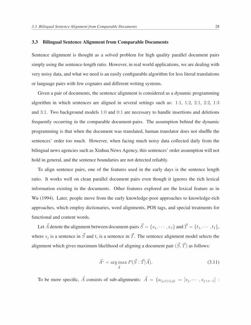
3.3. Bilingual Sentence Alignment from Comparable Documents 28
3.3 Bilingual Sentence Alignment from Comparable Documents
Sentence alignment is thought as a solved problem for high quality parallel document pairs
simply using the sentence-length ratio. However, in real world applications, we are dealing with
very noisy data, and what we need is an easily configurable algorithm for less literal translations
or language pairs with few cognates and different writing systems.
Given a pair of documents, the sentence alignment is considered as a dynamic programming
algorithm in which sentences are aligned in several settings such as: 1:1, 1:2, 2:1, 2:2, 1:3
and 3:1. Two background models 1:0 and 0:1 are necessary to handle insertions and deletions
frequently occurring in the comparable document-pairs. The assumption behind the dynamic
programming is that when the document was translated, human translator does not shuffle the
sentences’ order too much. However, when facing much noisy data collected daily from the
bilingual news agencies such as Xinhua News Agency, this sentences’ order assumption will not
hold in general, and the sentence boundaries are not detected reliably.
To align sentence pairs, one of the features used in the early days is the sentence length
ratio. It works well on clean parallel document pairs even though it ignores the rich lexical
information existing in the documents. Other features explored are the lexical feature as in
Wu (1994). Later, people move from the early knowledge-poor approaches to knowledge-rich
approaches, which employ dictionaries, word alignments, POS tags, and special treatments for
functional and content words.
Let ~A denote the alignment between document-pairs ~S = {s1, · · · , sJ} and ~T = {t1, · · · , tI},
where sj is a sentence in ~S and ti is a sentence in ~T . The sentence alignment model selects the
alignment which gives maximum likelihood of aligning a document pair (~S, ~T ) as follows:
~A∗ = arg max~A
P (~S : ~T | ~A). (3.11)
To be more specific, ~A consists of sub-alignments: ~A = {a(j,x):(i,y) = [sj, · · · , sj+x−1] :
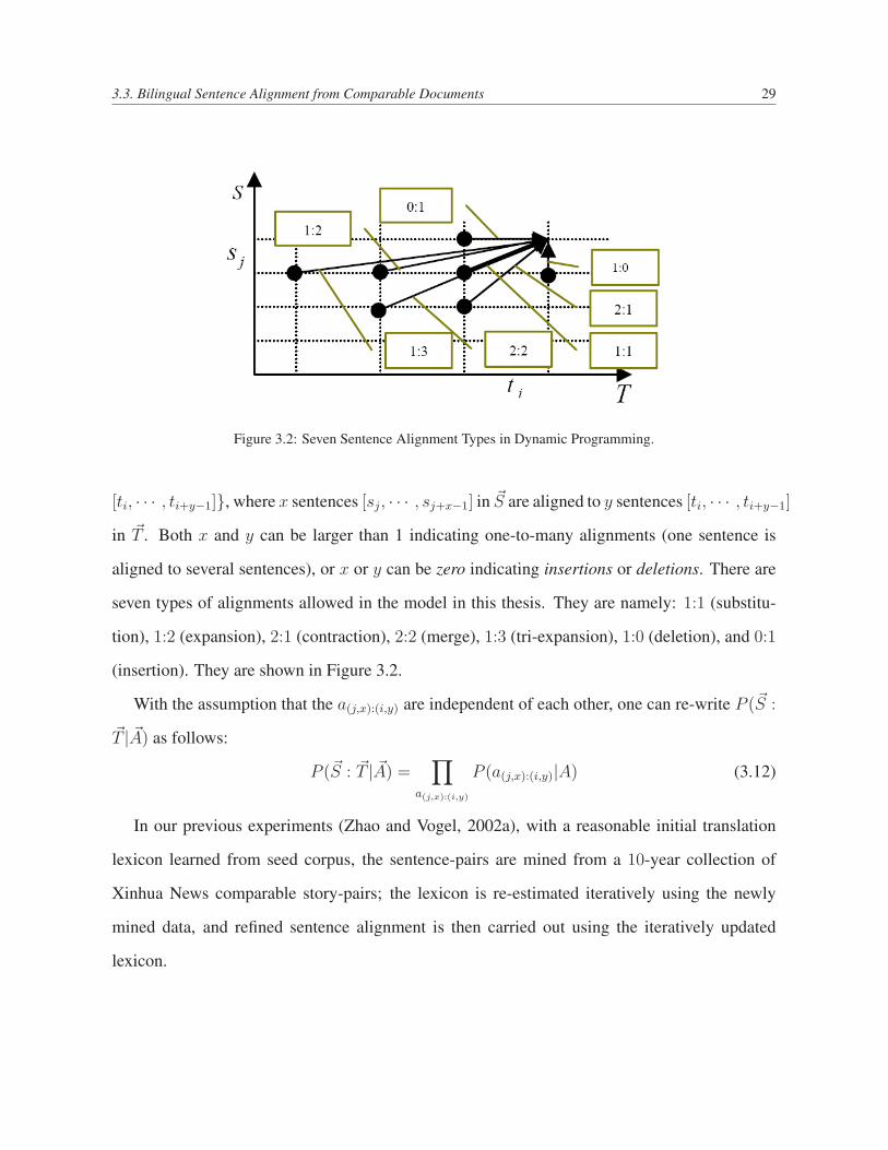
3.3. Bilingual Sentence Alignment from Comparable Documents 29
Figure 3.2: Seven Sentence Alignment Types in Dynamic Programming.
[ti, · · · , ti+y−1]}, where x sentences [sj, · · · , sj+x−1] in ~S are aligned to y sentences [ti, · · · , ti+y−1]
in ~T . Both x and y can be larger than 1 indicating one-to-many alignments (one sentence is
aligned to several sentences), or x or y can be zero indicating insertions or deletions. There are
seven types of alignments allowed in the model in this thesis. They are namely: 1:1 (substitu-
tion), 1:2 (expansion), 2:1 (contraction), 2:2 (merge), 1:3 (tri-expansion), 1:0 (deletion), and 0:1
(insertion). They are shown in Figure 3.2.
With the assumption that the a(j,x):(i,y) are independent of each other, one can re-write P (~S :
~T | ~A) as follows:
P (~S : ~T | ~A) =∏
a(j,x):(i,y)
P (a(j,x):(i,y)|A) (3.12)
In our previous experiments (Zhao and Vogel, 2002a), with a reasonable initial translation
lexicon learned from seed corpus, the sentence-pairs are mined from a 10-year collection of
Xinhua News comparable story-pairs; the lexicon is re-estimated iteratively using the newly
mined data, and refined sentence alignment is then carried out using the iteratively updated
lexicon.

3.4. Experiments 30
3.4 Experiments
In our experiments, we applied our proposed document alignment models in section 3.2 on
the ten-year’s collection of Xinhua news data to get the parallel documents first; the sentence-
alignment was then applied to extract the candidate parallel sentence-pairs; optimization and
filtering were applied to refine the final aligned sentence-pairs, which were released under LDC
catalog number LDC2003E18.
3.4.1 Mining from Web-collection for Comparable Documents
Experiments for the above mentioned Full-text alignment models showed the effectiveness for
document-pairs alignment using the data collected on Jan. 1st, 2000 published by Xinhua News
Agency in Chinese and English languages. There are 214 Chinese stories and 168 English stories
released on that day. We hand-labeled the data and found 26 document-pairs to be truly parallel
to each other.
As discussed in section 3.2, that the parallel story alignment can be considered as known-item
retrieval: each Chinese story has either none or exactly one parallel English story. The known-
item retrieval approach is well-suited to this task. Two evaluation measures can be applied for
this kind of problem:
• Rank of the known-item in an N-best list;
• Mean-reciprocal rank measure, which is the mean of the reciprocal of the rank at which the
known-item was found.
The first one gives close and detailed evaluations, and the second one gives a single value sum-
mary, which is in fact the average precision. We use these two measures together in our experi-
ments.
Standard pseudo-query retrieval, detailed in section 3.2.1 is carried out using the Lemur
Toolkit (http://www.lemurproject.org/). The pseudo-query is generated using the top-3 trans-
lation words from each word in a Chinese story. Two translation models are trained using the
3.4. Experiments 31
Hong Kong news data, one from English to Chinese and vice versa for alignment Model-A and
Model-B, respectively. The simple TF.IDF Okapi and LM-JM are compared with the two align-
ment models as shown in Figure 3.3. Table 3.1 gives the numbers of correctly retrieved items at
ranks up to 3. The mean-reciprocal rank is also shown in the bottom row.
Figure 3.3: Cumulative percentage of parallel stories found at each rank for Known-Item retrieval
In Figure 3.3, the models were evaluated for the cumulative percentage of parallel stories
found at each rank. On the x-axis is the rank of the founded parallel documents, on the y-axis is
the cumulative percentage of the found parallel document-pairs. It shows that both of the align-
ment models have better performances than the simple pseudo-query model based approaches.
Rank M-A M-B TFIDF Okapi LM-JM1 18 20 12 16 142 21 23 18 19 183 22 23 19 21 19
1/r 0.158 0.306 0.131 0.150 0.171
Table 3.1: Mean reciprocal rank and known items at the raw rank.
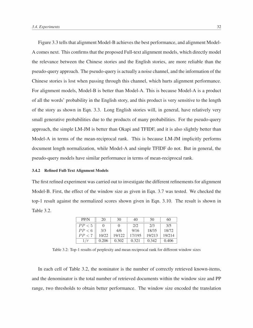
3.4. Experiments 32
Figure 3.3 tells that alignment Model-B achieves the best performance, and alignment Model-
A comes next. This confirms that the proposed Full-text alignment models, which directly model
the relevance between the Chinese stories and the English stories, are more reliable than the
pseudo-query approach. The pseudo-query is actually a noise channel, and the information of the
Chinese stories is lost when passing through this channel, which hurts alignment performance.
For alignment models, Model-B is better than Model-A. This is because Model-A is a product
of all the words’ probability in the English story, and this product is very sensitive to the length
of the story as shown in Eqn. 3.3. Long English stories will, in general, have relatively very
small generative probabilities due to the products of many probabilities. For the pseudo-query
approach, the simple LM-JM is better than Okapi and TFIDF, and it is also slightly better than
Model-A in terms of the mean-reciprocal rank. This is because LM-JM implicitly performs
document length normalization, while Model-A and simple TFIDF do not. But in general, the
pseudo-query models have similar performance in terms of mean-reciprocal rank.
3.4.2 Refined Full-Text Alignment Models
The first refined experiment was carried out to investigate the different refinements for alignment
Model-B. First, the effect of the window size as given in Eqn. 3.7 was tested. We checked the
top-1 result against the normalized scores shown given in Eqn. 3.10. The result is shown in
Table 3.2.
PP/N 20 30 40 50 60PP < 5 0 0 2/2 2/3 3/5PP < 6 3/3 4/6 9/16 18/35 18/72PP < 7 10/22 19/122 17/195 19/213 19/214
1/r 0.206 0.302 0.321 0.342 0.406
Table 3.2: Top-1 results of perplexity and mean reciprocal rank for different window sizes
In each cell of Table 3.2, the nominator is the number of correctly retrieved known-items,
and the denominator is the total number of retrieved documents within the window size and PP
range, two thresholds to obtain better performance. The window size encoded the translation
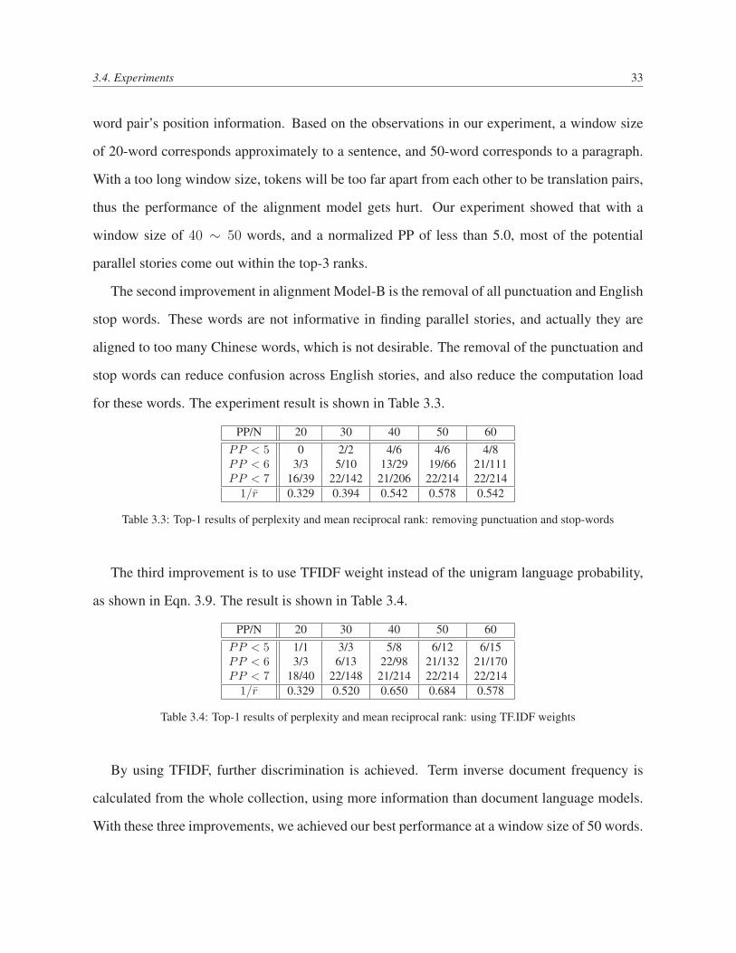
3.4. Experiments 33
word pair’s position information. Based on the observations in our experiment, a window size
of 20-word corresponds approximately to a sentence, and 50-word corresponds to a paragraph.
With a too long window size, tokens will be too far apart from each other to be translation pairs,
thus the performance of the alignment model gets hurt. Our experiment showed that with a
window size of 40 ∼ 50 words, and a normalized PP of less than 5.0, most of the potential
parallel stories come out within the top-3 ranks.
The second improvement in alignment Model-B is the removal of all punctuation and English
stop words. These words are not informative in finding parallel stories, and actually they are
aligned to too many Chinese words, which is not desirable. The removal of the punctuation and
stop words can reduce confusion across English stories, and also reduce the computation load
for these words. The experiment result is shown in Table 3.3.
PP/N 20 30 40 50 60PP < 5 0 2/2 4/6 4/6 4/8PP < 6 3/3 5/10 13/29 19/66 21/111PP < 7 16/39 22/142 21/206 22/214 22/214
1/r 0.329 0.394 0.542 0.578 0.542
Table 3.3: Top-1 results of perplexity and mean reciprocal rank: removing punctuation and stop-words
The third improvement is to use TFIDF weight instead of the unigram language probability,
as shown in Eqn. 3.9. The result is shown in Table 3.4.
PP/N 20 30 40 50 60PP < 5 1/1 3/3 5/8 6/12 6/15PP < 6 3/3 6/13 22/98 21/132 21/170PP < 7 18/40 22/148 21/214 22/214 22/214
1/r 0.329 0.520 0.650 0.684 0.578
Table 3.4: Top-1 results of perplexity and mean reciprocal rank: using TF.IDF weights
By using TFIDF, further discrimination is achieved. Term inverse document frequency is
calculated from the whole collection, using more information than document language models.
With these three improvements, we achieved our best performance at a window size of 50 words.
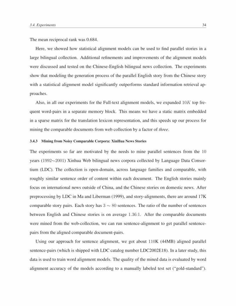
3.4. Experiments 34
The mean reciprocal rank was 0.684.
Here, we showed how statistical alignment models can be used to find parallel stories in a
large bilingual collection. Additional refinements and improvements of the alignment models
were discussed and tested on the Chinese-English bilingual news collection. The experiments
show that modeling the generation process of the parallel English story from the Chinese story
with a statistical alignment model significantly outperforms standard information retrieval ap-
proaches.
Also, in all our experiments for the Full-text alignment models, we expanded 10K top fre-
quent word-pairs in a separate memory block. This means we have a static matrix embedded
in a sparse matrix for the translation lexicon representation, and this speeds up our process for
mining the comparable documents from web collection by a factor of three.
3.4.3 Mining from Noisy Comparable Corpora: XinHua News Stories
The experiments so far are motivated by the needs to mine parallel sentences from the 10
years (1992∼2001) Xinhua Web bilingual news corpora collected by Language Data Consor-
tium (LDC). The collection is open-domain, across language families and comparable, with
roughly similar sentence order of content within each document. The English stories mainly
focus on international news outside of China, and the Chinese stories on domestic news. After
preprocessing by LDC in Ma and Liberman (1999), and story-alignments, there are around 17K
comparable story pairs. Each story has 3 ∼ 80 sentences. The ratio of the number of sentences
between English and Chinese stories is on average 1.36:1. After the comparable documents
were mined from the web-collection, we can run sentence-alignment to get parallel sentence-
pairs from the aligned comparable document-pairs.
Using our approach for sentence alignment, we got about 110K (44MB) aligned parallel
sentence-pairs (which is shipped with LDC catalog number LDC2002E18). In a later study, this
data is used to train word alignment models. The quality of the mined data is evaluated by word
alignment accuracy of the models according to a manually labeled test set (“gold-standard”).
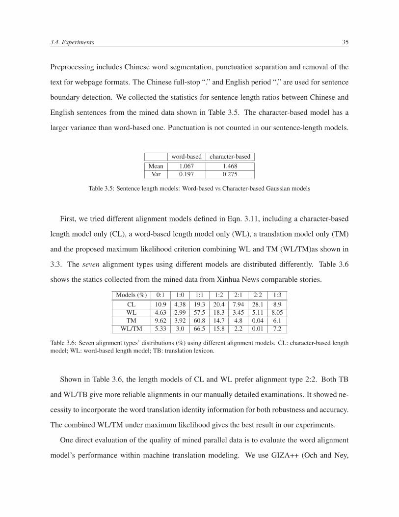
3.4. Experiments 35
Preprocessing includes Chinese word segmentation, punctuation separation and removal of the
text for webpage formats. The Chinese full-stop “.” and English period “.” are used for sentence
boundary detection. We collected the statistics for sentence length ratios between Chinese and
English sentences from the mined data shown in Table 3.5. The character-based model has a
larger variance than word-based one. Punctuation is not counted in our sentence-length models.
word-based character-basedMean 1.067 1.468Var 0.197 0.275
Table 3.5: Sentence length models: Word-based vs Character-based Gaussian models
First, we tried different alignment models defined in Eqn. 3.11, including a character-based
length model only (CL), a word-based length model only (WL), a translation model only (TM)
and the proposed maximum likelihood criterion combining WL and TM (WL/TM)as shown in
3.3. The seven alignment types using different models are distributed differently. Table 3.6
shows the statics collected from the mined data from Xinhua News comparable stories.
Models (%) 0:1 1:0 1:1 1:2 2:1 2:2 1:3CL 10.9 4.38 19.3 20.4 7.94 28.1 8.9WL 4.63 2.99 57.5 18.3 3.45 5.11 8.05TM 9.62 3.92 60.8 14.7 4.8 0.04 6.1
WL/TM 5.33 3.0 66.5 15.8 2.2 0.01 7.2
Table 3.6: Seven alignment types’ distributions (%) using different alignment models. CL: character-based lengthmodel; WL: word-based length model; TB: translation lexicon.
Shown in Table 3.6, the length models of CL and WL prefer alignment type 2:2. Both TB
and WL/TB give more reliable alignments in our manually detailed examinations. It showed ne-
cessity to incorporate the word translation identity information for both robustness and accuracy.
The combined WL/TM under maximum likelihood gives the best result in our experiments.
One direct evaluation of the quality of mined parallel data is to evaluate the word alignment
model’s performance within machine translation modeling. We use GIZA++ (Och and Ney,

3.4. Experiments 36
Alignment Types (%) 0:1 1:0 1:1 1:2 2:1 2:2 1:3Iter 1 5.33 3.00 66.5 15.8 2.20 0.01 7.21Iter 2 4.86 2.69 66.9 16.0 2.26 0.01 7.29Iter 3 4.81 2.65 66.6 16.3 2.38 0.01 7.26Iter 4 4.81 2.64 66.6 16.2 2.39 0.01 7.28
Table 3.7: Alignment types (%) changes over iterations
2003) to build the translation models up to IBM Model-3. Word alignment accuracy is calcu-
lated according to a hand-aligned 365 sentence-pairs test set containing 4, 094 word-to-word
alignments. Table 3.8 shows the word alignment accuracy of translation models learned from
the mined parallel data.
Baseline Model-1 Model-2 Model-3Precision 43.43% 44.98% 43.65%
Recall 50.98% 53.81% 49.66%F 46.90% 49.00% 46.46%
Mined data Model-1 Model-2 Model-3Precision 48.94% 48.88% 48.88%
Recall 58.97% 58.55% 56.84%F 53.49% 53.28% 52.56%
Table 3.8: Word alignment accuracy using the mined Data from XinHua News Stories from 1992∼2001.
The baseline models were learned using the Hong Kong News data set, which contains 290K
parallel sentence pairs from LDC. The mined data are 57K sentence pairs (with pp < 5.0)
selected after four iterations; the best quality we get from all the four iterations. There is a
consistent improvement for all the three word alignment models. The F-measure of Model-1
has a 14.05% relative improvement, showing better vocabulary coverage and the high parallel
quality of the data mined using the proposed models.
3.4.4 Mining from High-Quality Parallel Corpora: FBIS Corpora
FBIS data (LDC2003E14) is a collection of translated newswire documents published by major
news agencies from three representative locations: Beijing, Taipei and Hong Kong. The doc-
uments are translated by professional translators, and are aligned at the document-level. We
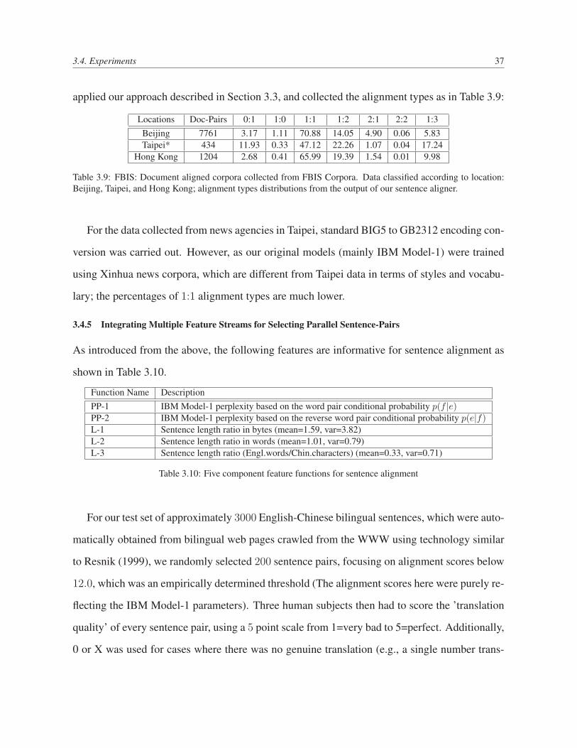
3.4. Experiments 37
applied our approach described in Section 3.3, and collected the alignment types as in Table 3.9:
Locations Doc-Pairs 0:1 1:0 1:1 1:2 2:1 2:2 1:3Beijing 7761 3.17 1.11 70.88 14.05 4.90 0.06 5.83Taipei* 434 11.93 0.33 47.12 22.26 1.07 0.04 17.24
Hong Kong 1204 2.68 0.41 65.99 19.39 1.54 0.01 9.98
Table 3.9: FBIS: Document aligned corpora collected from FBIS Corpora. Data classified according to location:Beijing, Taipei, and Hong Kong; alignment types distributions from the output of our sentence aligner.
For the data collected from news agencies in Taipei, standard BIG5 to GB2312 encoding con-
version was carried out. However, as our original models (mainly IBM Model-1) were trained
using Xinhua news corpora, which are different from Taipei data in terms of styles and vocabu-
lary; the percentages of 1:1 alignment types are much lower.
3.4.5 Integrating Multiple Feature Streams for Selecting Parallel Sentence-Pairs
As introduced from the above, the following features are informative for sentence alignment as
shown in Table 3.10.
Function Name DescriptionPP-1 IBM Model-1 perplexity based on the word pair conditional probability p(f |e)PP-2 IBM Model-1 perplexity based on the reverse word pair conditional probability p(e|f)L-1 Sentence length ratio in bytes (mean=1.59, var=3.82)L-2 Sentence length ratio in words (mean=1.01, var=0.79)L-3 Sentence length ratio (Engl.words/Chin.characters) (mean=0.33, var=0.71)
Table 3.10: Five component feature functions for sentence alignment
For our test set of approximately 3000 English-Chinese bilingual sentences, which were auto-
matically obtained from bilingual web pages crawled from the WWW using technology similar
to Resnik (1999), we randomly selected 200 sentence pairs, focusing on alignment scores below
12.0, which was an empirically determined threshold (The alignment scores here were purely re-
flecting the IBM Model-1 parameters). Three human subjects then had to score the ’translation
quality’ of every sentence pair, using a 5 point scale from 1=very bad to 5=perfect. Additionally,
0 or X was used for cases where there was no genuine translation (e.g., a single number trans-

3.4. Experiments 38
lated to itself), or where both sentences were from the same language. We further excluded too
short sentences from consideration and evaluated 168 remaining hand labeled sentences.
The correlation coefficients (Pearson r) between human subjects were as follows (all are
statistically significant) in Table 3.11:
H2 H3H1 0.786 0.615H2 — 0.568
Table 3.11: Correlation between Human Subjects
Correlation table of the five component feature function alignment scores based on Model X
and human subjects’ translation quality scores are also computed as shown in the Table 3.12:
Model human-1 human-2 human-3PP-1 .57 .53 .32PP-2 .60 .58 .46L-1 .42 .41 .30L-2 .46 .41 .40L-3 .40 .38 .29
Regression model .72 .68 .53
Table 3.12: Correlation between customization models and human subjects
The regression model here is the standard linear regression using the observations (5-scale
scores) from three human subjects. The averaged performance of the regression model is shown
in the bottom line in the above table. The average correlation varies from 0.53 to 0.72, which
shows the regression model is a good approximation of the human judgment.
We also performed correlation experiments with varied numbers of training sentences from
either Human-1/Human-2/Human-3 or from all of the three human subjects. We picked the first
30/60/90/120 sentence pairs for training and saved the last 48 sentence pairs for testing. The
average performance of the regression model is shown in Table 3.13:
The average correlation of the regression models shown here increased noticeably when the
training set was increased from 30 sentence pairs to 90 sentence pairs. More sentence pairs
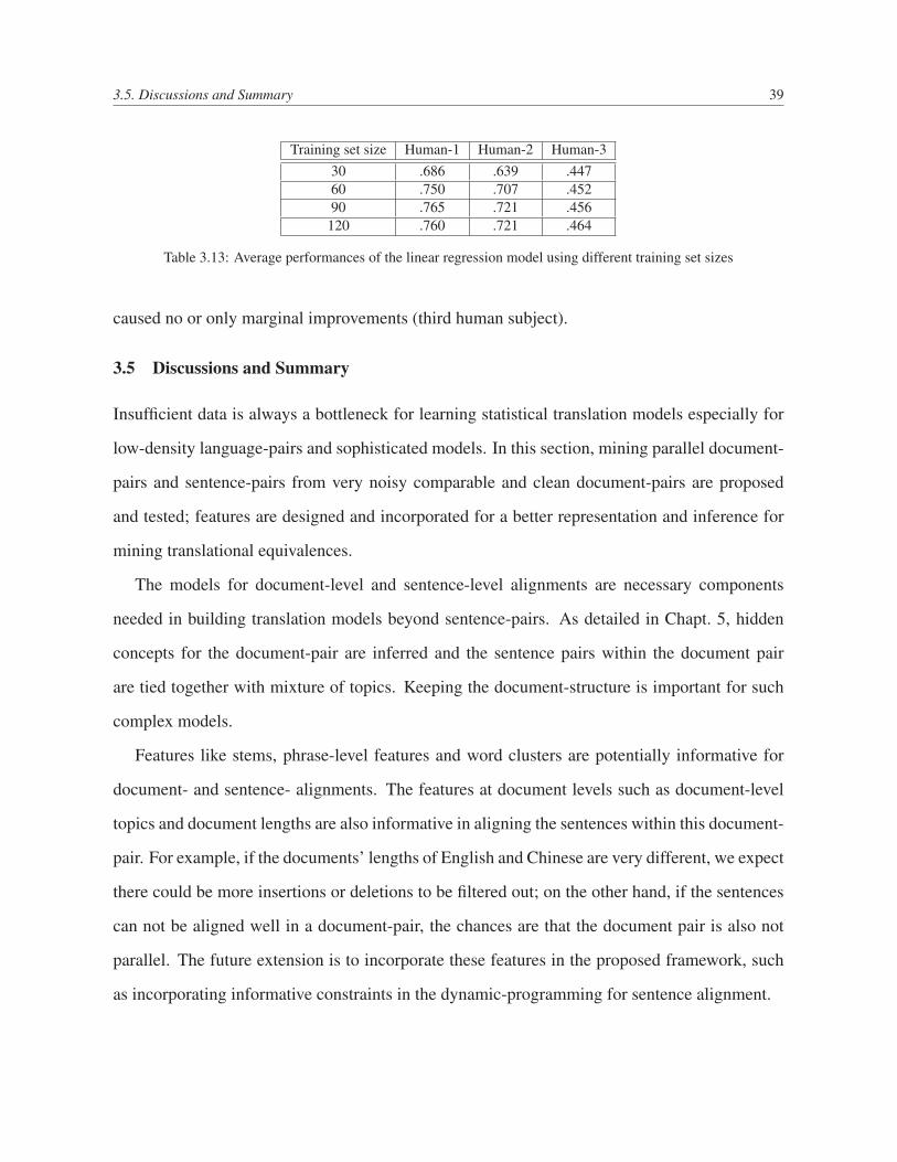
3.5. Discussions and Summary 39
Training set size Human-1 Human-2 Human-330 .686 .639 .44760 .750 .707 .45290 .765 .721 .456
120 .760 .721 .464
Table 3.13: Average performances of the linear regression model using different training set sizes
caused no or only marginal improvements (third human subject).
3.5 Discussions and Summary
Insufficient data is always a bottleneck for learning statistical translation models especially for
low-density language-pairs and sophisticated models. In this section, mining parallel document-
pairs and sentence-pairs from very noisy comparable and clean document-pairs are proposed
and tested; features are designed and incorporated for a better representation and inference for
mining translational equivalences.
The models for document-level and sentence-level alignments are necessary components
needed in building translation models beyond sentence-pairs. As detailed in Chapt. 5, hidden
concepts for the document-pair are inferred and the sentence pairs within the document pair
are tied together with mixture of topics. Keeping the document-structure is important for such
complex models.
Features like stems, phrase-level features and word clusters are potentially informative for
document- and sentence- alignments. The features at document levels such as document-level
topics and document lengths are also informative in aligning the sentences within this document-
pair. For example, if the documents’ lengths of English and Chinese are very different, we expect
there could be more insertions or deletions to be filtered out; on the other hand, if the sentences
can not be aligned well in a document-pair, the chances are that the document pair is also not
parallel. The future extension is to incorporate these features in the proposed framework, such
as incorporating informative constraints in the dynamic-programming for sentence alignment.

Chapter 4
Leveraging Bilingual Feature Streams
The word alignment and phrase alignment are building blocks for state-of-the-art statistical
phrase-based machine translation systems. Information utilized by human translators is very
broad, but our current models on top of HMM and IBM models are not yet capable of capturing
such phenomena. We are aiming at leveraging informative feature streams which can be em-
bedded naturally in alignment models for word and phrase-alignment to enrich the structures for
translations.
A few previous approaches were designed for enriching the dependencies for alignment mod-
els. For example, the jump-table proposed in hidden Markov model (HMM) (Vogel et al., 1996)
implemented the assumption that words “close-in-source” will be aligned to words “close-in-
target”. It was then further extended with dependency using monolingual word-classes in Och
and Ney (2003) and POS tags in Toutanova et al. (2002). The context features of dependency
in Cherry and Lin (2003) modeled two types of dependencies: adjacency features surround-
ing alignment links, and dependency features based on English parsing trees from monolingual
parsers. The model’s performance is shown to be close to a lemmatized bi-directional IBM
Model-4 in the same shared tasks of Dejean et al. (2003). Some information streams have been
tested to be useful in terms of preprocessing or post-processing besides Dejean et al. (2003). This
40
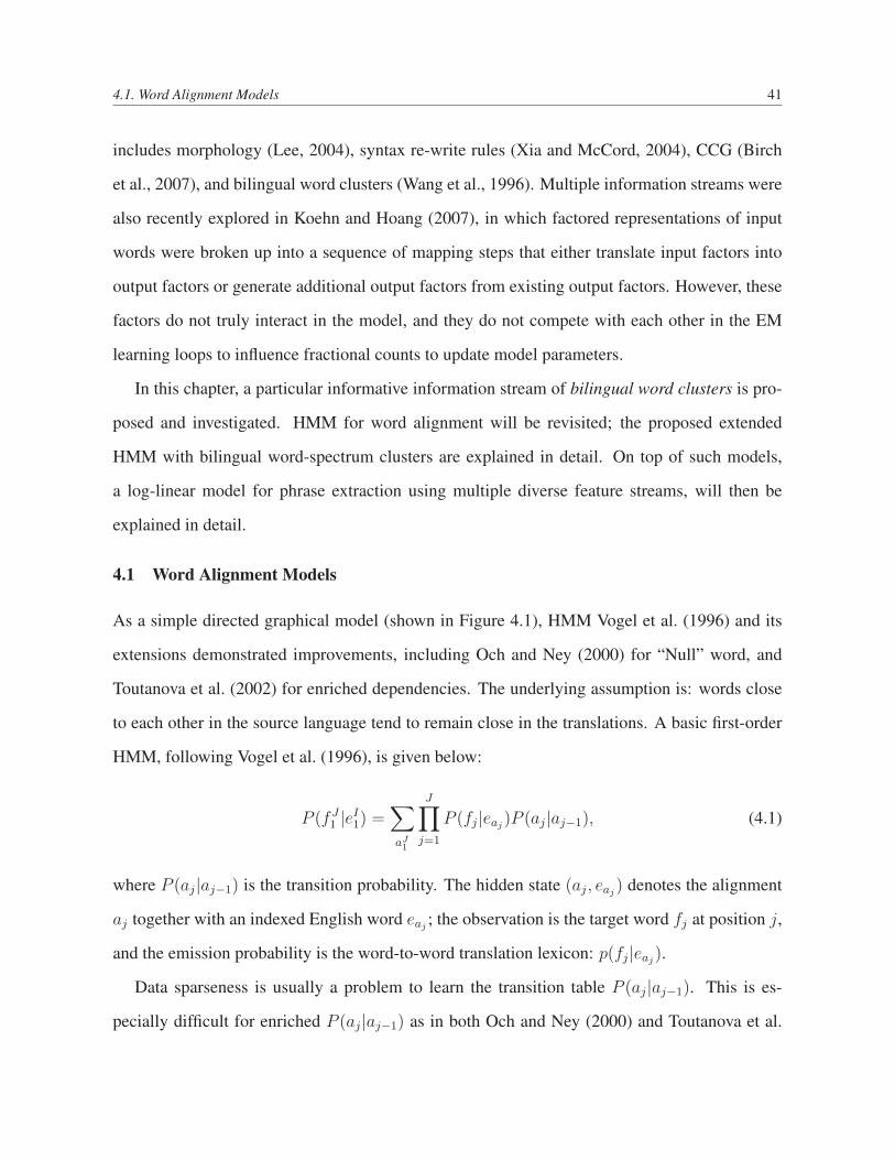
4.1. Word Alignment Models 41
includes morphology (Lee, 2004), syntax re-write rules (Xia and McCord, 2004), CCG (Birch
et al., 2007), and bilingual word clusters (Wang et al., 1996). Multiple information streams were
also recently explored in Koehn and Hoang (2007), in which factored representations of input
words were broken up into a sequence of mapping steps that either translate input factors into
output factors or generate additional output factors from existing output factors. However, these
factors do not truly interact in the model, and they do not compete with each other in the EM
learning loops to influence fractional counts to update model parameters.
In this chapter, a particular informative information stream of bilingual word clusters is pro-
posed and investigated. HMM for word alignment will be revisited; the proposed extended
HMM with bilingual word-spectrum clusters are explained in detail. On top of such models,
a log-linear model for phrase extraction using multiple diverse feature streams, will then be
explained in detail.
4.1 Word Alignment Models
As a simple directed graphical model (shown in Figure 4.1), HMM Vogel et al. (1996) and its
extensions demonstrated improvements, including Och and Ney (2000) for “Null” word, and
Toutanova et al. (2002) for enriched dependencies. The underlying assumption is: words close
to each other in the source language tend to remain close in the translations. A basic first-order
HMM, following Vogel et al. (1996), is given below:
P (fJ1 |eI
1) =∑
aJ1
J∏j=1
P (fj|eaj)P (aj|aj−1), (4.1)
where P (aj|aj−1) is the transition probability. The hidden state (aj, eaj) denotes the alignment
aj together with an indexed English word eaj; the observation is the target word fj at position j,
and the emission probability is the word-to-word translation lexicon: p(fj|eaj).
Data sparseness is usually a problem to learn the transition table P (aj|aj−1). This is es-
pecially difficult for enriched P (aj|aj−1) as in both Och and Ney (2000) and Toutanova et al.
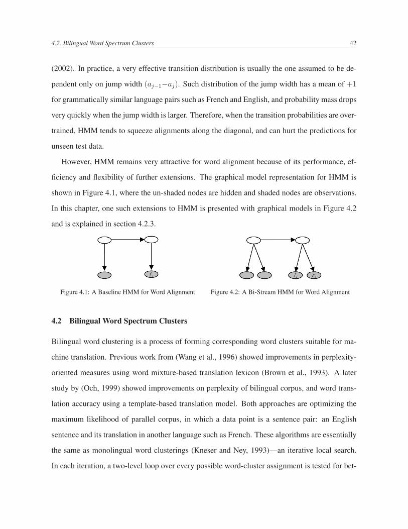
4.2. Bilingual Word Spectrum Clusters 42
(2002). In practice, a very effective transition distribution is usually the one assumed to be de-
pendent only on jump width (aj−1−aj). Such distribution of the jump width has a mean of +1
for grammatically similar language pairs such as French and English, and probability mass drops
very quickly when the jump width is larger. Therefore, when the transition probabilities are over-
trained, HMM tends to squeeze alignments along the diagonal, and can hurt the predictions for
unseen test data.
However, HMM remains very attractive for word alignment because of its performance, ef-
ficiency and flexibility of further extensions. The graphical model representation for HMM is
shown in Figure 4.1, where the un-shaded nodes are hidden and shaded nodes are observations.
In this chapter, one such extensions to HMM is presented with graphical models in Figure 4.2
and is explained in section 4.2.3.
Figure 4.1: A Baseline HMM for Word Alignment Figure 4.2: A Bi-Stream HMM for Word Alignment
4.2 Bilingual Word Spectrum Clusters
Bilingual word clustering is a process of forming corresponding word clusters suitable for ma-
chine translation. Previous work from (Wang et al., 1996) showed improvements in perplexity-
oriented measures using word mixture-based translation lexicon (Brown et al., 1993). A later
study by (Och, 1999) showed improvements on perplexity of bilingual corpus, and word trans-
lation accuracy using a template-based translation model. Both approaches are optimizing the
maximum likelihood of parallel corpus, in which a data point is a sentence pair: an English
sentence and its translation in another language such as French. These algorithms are essentially
the same as monolingual word clusterings (Kneser and Ney, 1993)—an iterative local search.
In each iteration, a two-level loop over every possible word-cluster assignment is tested for bet-
4.2. Bilingual Word Spectrum Clusters 43
ter likelihood change. This kind of approach has two drawbacks: first it can get stuck in local
optima; second, the clustering of English and the other language are basically two separated
optimization processes, and cluster-level translation is modeled loosely. These drawbacks make
their approaches generally not very effective in improving translation models.
In this Chapter, a variant of the spectral clustering algorithm (Ng et al., 2001) is proposed
for bilingual word clustering. Given parallel corpus, first, the word’s bilingual context is used
directly as features — for instance, each English word is represented by its bilingual word trans-
lation candidates. Second, latent eigenstructure analysis is carried out in this bilingual feature
space, which leads to clusters of words with similar translations. Essentially an affinity matrix is
computed using these cross-lingual features. It is then decomposed into two sub-spaces, which
are meaningful for translation tasks: the left subspace corresponds to the representation of words
in English vocabulary, and the right sub-space corresponds to words in French. Each eigenvector
is considered as one bilingual concept, and the bilingual clusters are considered to be its realiza-
tions in two languages. Finally, a general K-means clustering algorithm is used to find out word
clusters in the two sub-spaces.
In bilingual word clustering, the task is to build word clusters F and E to form partitions of
the vocabularies of the two languages respectively. The two partitions for the vocabularies of F
and E are aimed to be suitable for machine translation in the sense that the cluster/partition level
translation equivalence is reliable and focused to handle data sparseness; the translation model
using these clusters explains the parallel corpus {(fJ1 , eI
1)} better in terms of perplexity or joint
likelihood.
4.2. Bilingual Word Spectrum Clusters 44
4.2.1 From Monolingual to Bilingual
To infer bilingual word clusters of (F, E), one can optimize the joint probability of the parallel
corpus {(fJ1 , eI
1)} using the clusters as follows:
(F, E) = arg max(F,E)
P (fJ1 , eI
1|F,E)
= arg max(F,E)
P (eI1|E)P (fJ
1 |eI1, F, E). (4.2)
Eqn. 4.2 separates the optimization process into two parts: the monolingual part for E, and the
bilingual part for F given fixed E. The monolingual part is considered as a prior probability:P (eI1|E),
and E can be inferred using corpus bigram statistics in the following equation:
E = arg max{E}
P (eI1|E)
= arg max{E}
I∏i=1
P (Ei|Ei−1)P (ei|Ei). (4.3)
We need to fix the number of clusters beforehand, otherwise the optimum is reached when each
word is a class of its own. There exists efficient leave-one-out style algorithm (Kneser and Ney,
1993), which can automatically determine the number of clusters.
For the bilingual part P (fJ1 |eI
1, F, E), we can slightly modify the same algorithm as in
(Kneser and Ney, 1993). Given the word alignment {aJ1} between fJ
1 and eI1 collected from
the Viterbi path in HMM-based translation model, we can infer F as follows:
F = arg max{F}
P (fJ1 |eI
1, F, E)
= arg max{F}
J∏j=1
P (Fj|Eaj)P (fj|Fj). (4.4)
Overall, this bilingual word clustering algorithm is essentially a two-step approach. In the first
step, E is inferred by optimizing the monolingual likelihood of English data, and secondly F is
4.2. Bilingual Word Spectrum Clusters 45
inferred by optimizing the bilingual part without changing E. In this way, the algorithm is easy
to implement without much change from the monolingual counterpart.
This approach was shown to give the best results in (Och, 1999). We use it as our baseline to
compare with.
4.2.2 Bilingual Word Spectral Clustering
Instead of using word alignment to bridge the parallel sentence pair, and optimize the likelihood
in two separate steps, we develop an alignment-free algorithm using a variant of spectral cluster-
ing algorithm. The goal is to build high cluster-level translation quality suitable for translation
modeling, and at the same time maintain high intra-cluster similarity , and low inter-cluster
similarity clusters for both F and E.
Notations
We define the vocabulary VF as the French vocabulary with a size of |VF |; VE as the English
vocabulary with size of |VE|. A co-occurrence matrix C{F,E} is built with |VF | rows and |VE|columns; each element represents the co-occurrence counts of the corresponding French word
fj and English word ei. In this way, each French word forms a row vector with a dimension of
|VE|, and each coordinate is a co-occurring English word. The elements in the vector are the
co-occurrence counts. We can also view each column as a vector for English word, and we’ll
have similar interpretations as above.
Algorithm
With C{F,E}, we can infer two affinity matrixes as follows:
AE = CT{F,E}C{F,E}
AF = C{F,E}CT{F,E},
where AE is an |VE| × |VE| affinity matrix for English words, with rows and columns repre-
senting English words and each element the inner product between two English words column

4.2. Bilingual Word Spectrum Clusters 46
vectors. Correspondingly, AF is an affinity matrix of size |VF | × |VF | for French words with
similar definitions. Both AE and AF are symmetric and non-negative. Now we can compute the
eigenstructure for both AE and AF . In fact, the eigen vectors of the two are correspondingly the
right and left sub-spaces of the original co-occurrence matrix of C{F,E}, respectively. This can
be computed using singular value decomposition (SVD): C{F,E} = USV T , AE = V S2V T , and
AF = US2UT , where U is the left sub-space, and V the right sub-space of the co-occurrence
matrix C{F,E}. S is a diagonal matrix, with the singular values ranked from large to small along
the diagonal. Obviously, the left sub-space U is the eigenstructure for AF ; the right sub-space V
is the eigenstructure for AE .
By choosing the top K singular values (the square root of the eigen values for both AE and
AF ), the sub-spaces will be reduced to: U|VF |×K and V|VE |×K , respectively. Based on these
subspaces, we can carry out K-means or other clustering algorithms to infer word clusters for
both languages. Our algorithm goes as follows:
• Initialize bilingual co-occurrence matrix C{F,E} with rows representing French words, and
columns English words. Cji is the co-occurrence raw counts of French word fj and English
word ei;
• Form the affinity matrix AE = CT{F,E}C{F,E} and AF = CT
{F,E}C{F,E}. Kernels can also
be applied here such as AE = exp(C{F,E}CT
{F,E}σ2 ) for English words. Set AEii = 0 and
AF ii = 0, and normalize each row to be unit length;
• Compute the eigen structure of the normalized matrix AE , and find the k largest eigen
vectors: v1, v2, ..., vk; Similarly, find the k largest eigen vectors of AF : u1, u2, ..., uk;
• Stack the k eigenvectors of v1, v2, ..., vk in the columns of YE , and stack the eigenvectors
u1, u2, ..., uk in the columns for YF ; Normalize rows of both YE and YF to have unit length.
YE is size of |VE| × k and YF is size of |VF | × k;
• Treat each row of YE as a point in R|VE |×k, and cluster them into K English word clusters
4.2. Bilingual Word Spectrum Clusters 47
using K-means. Treat each row of YF as a point in R|VF |×k, and cluster them into K French
word clusters.
• Finally, assign original word ei to cluster Ek if row i of the matrix YE is clustered as Ek;
similar assignments are for French words.
Here AE and AF are affinity matrixes of pair-wise inner products between the monolingual
words. The more similar the two words, the larger the value. In our implementations, we did not
apply a kernel function like the algorithm in (Ng et al., 2001). But the kernel function such as the
exponential function mentioned above can be applied here to control how rapidly the similarity
falls, using some carefully chosen scaling parameter.
Related Clustering Algorithms
The above algorithm is very close to the variants of a big family of the spectral clustering
algorithms introduced in (Meila and Shi, 2000) and studied in (Ng et al., 2001). Spectral clus-
tering refers to a class of techniques which rely on the eigenstructure of a similarity matrix to
partition points into disjoint clusters with high intra-cluster similarity and low inter-cluster sim-
ilarity. It’s shown to be computing the k-way normalized cut: K − trY T D− 12 AD− 1
2 Y for any
matrix Y ∈ RM×N . A is the affinity matrix, and Y in our algorithm corresponds to the subspaces
of U and V .
Experimentally, it has been observed that using more eigenvectors and directly computing a
k-way partitioning usually gives better performance. In our implementations, we used the top
500 eigen vectors to construct the subspaces of U and V for K-means clustering.
K-means
The K-means here can be considered as a post-processing step in our proposed bilingual word
clustering. For initial centroids, we first compute the center of the whole data set. The farthest
centroid from the center is then chosen to be the first initial centroid; and after that, the other
K-1 centroids are chosen one by one to well separate all the previous chosen centroids.

4.2. Bilingual Word Spectrum Clusters 48
The stopping criterion is: if the maximal change of the clusters’ centroids is less than the
threshold of 1e-3 between two iterations, the clustering algorithm then stops.
4.2.3 A Bi-Stream HMM
Let F denote the cluster mapping fj → F(fj), which assigns French word fj to its cluster ID
Fj = F(fj). Similarly E maps English word ei to its cluster ID of Ei = E(ei). In this section,
we assume each word belongs to one cluster only.
With bilingual word clusters, we can extend the HMM model in two ways. First, the jump
table is extended with clusters, so that the jump-distance depends on word cluster labels.
P (fJ1 |eI
1) =∑
aJ1
J∏j=1
P (fj|eaj) · P (aj|aj−1, E(eaj−1
), F(fj−1)), (4.5)
where E(eaj−1) and F(fj−1) are non-overlapping word clusters (Eaj−1
, Fj−1) for English and
French, respectively.
The second explicit way of utilizing bilingual word clusters can be considered as a two-stream
HMM as follows:
P (fJ1 , F J
1 |eI1, E
I1) =
∑
aJ1
J∏j=1
P (fj|eaj)P (Fj|Eaj
)P (aj|aj−1). (4.6)
This model introduces the translation of bilingual word clusters directly as an extra factor to
Eqn. 4.1. Intuitively, the role of this factor is to boost the translation probabilities for words
sharing the same concept (i.e., cluster label). This is a more expressive model because it models
both word and cluster level translation equivalences. Also, compared with the model in Eqn.
4.5, this model is easier to learn, as it uses two decoupled two-dimension tables (P (Fj|Eaj) and
P (aj|aj−1) ) instead of a four-dimension table of P (aj|aj−1, E(eaj−1), F(fj−1)).
However, we do not want this P (Fj|Eaj) to dominate the HMM transition structure, and the
observation probability of P (fj|eaj) during the EM iterations. Thus a uniform prior P (Fj) =
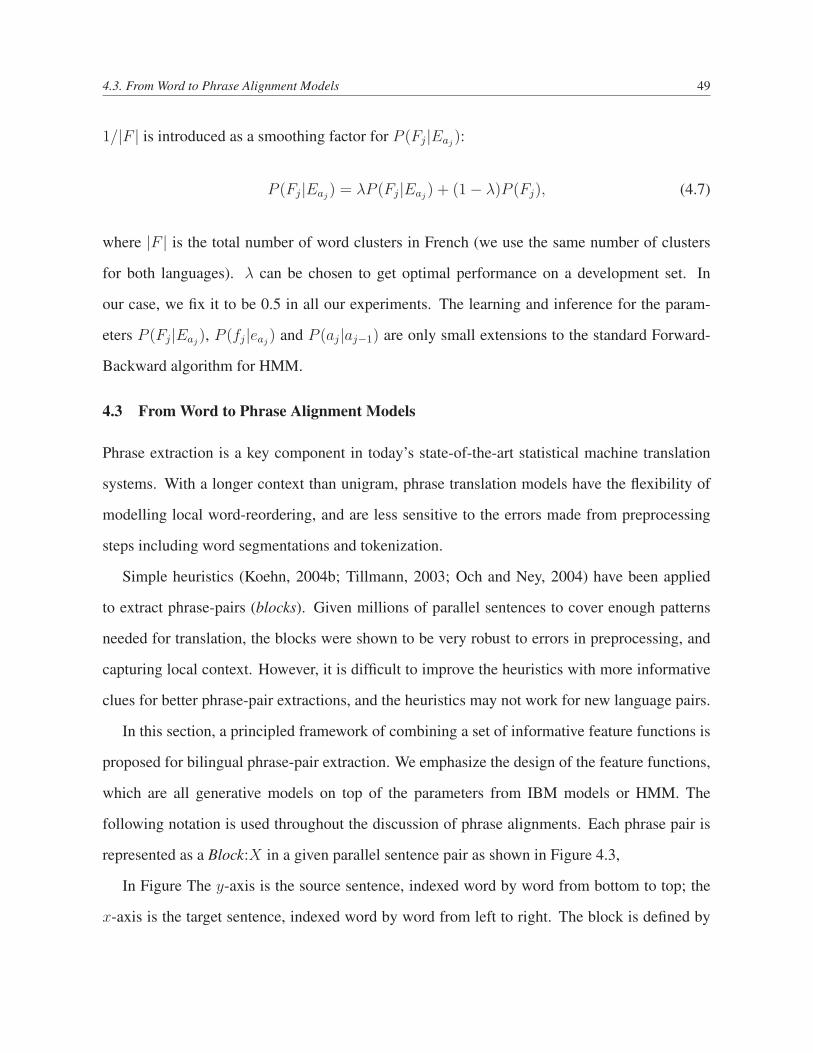
4.3. From Word to Phrase Alignment Models 49
1/|F | is introduced as a smoothing factor for P (Fj|Eaj):
P (Fj|Eaj) = λP (Fj|Eaj
) + (1− λ)P (Fj), (4.7)
where |F | is the total number of word clusters in French (we use the same number of clusters
for both languages). λ can be chosen to get optimal performance on a development set. In
our case, we fix it to be 0.5 in all our experiments. The learning and inference for the param-
eters P (Fj|Eaj), P (fj|eaj
) and P (aj|aj−1) are only small extensions to the standard Forward-
Backward algorithm for HMM.
4.3 From Word to Phrase Alignment Models
Phrase extraction is a key component in today’s state-of-the-art statistical machine translation
systems. With a longer context than unigram, phrase translation models have the flexibility of
modelling local word-reordering, and are less sensitive to the errors made from preprocessing
steps including word segmentations and tokenization.
Simple heuristics (Koehn, 2004b; Tillmann, 2003; Och and Ney, 2004) have been applied
to extract phrase-pairs (blocks). Given millions of parallel sentences to cover enough patterns
needed for translation, the blocks were shown to be very robust to errors in preprocessing, and
capturing local context. However, it is difficult to improve the heuristics with more informative
clues for better phrase-pair extractions, and the heuristics may not work for new language pairs.
In this section, a principled framework of combining a set of informative feature functions is
proposed for bilingual phrase-pair extraction. We emphasize the design of the feature functions,
which are all generative models on top of the parameters from IBM models or HMM. The
following notation is used throughout the discussion of phrase alignments. Each phrase pair is
represented as a Block:X in a given parallel sentence pair as shown in Figure 4.3,
In Figure The y-axis is the source sentence, indexed word by word from bottom to top; the
x-axis is the target sentence, indexed word by word from left to right. The block is defined by
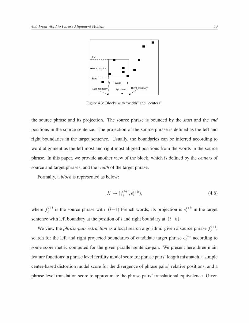
4.3. From Word to Phrase Alignment Models 50
Start
End
Right boundaryLeft boundary
Width
src center
tgt center
Figure 4.3: Blocks with “width” and “centers”
the source phrase and its projection. The source phrase is bounded by the start and the end
positions in the source sentence. The projection of the source phrase is defined as the left and
right boundaries in the target sentence. Usually, the boundaries can be inferred according to
word alignment as the left most and right most aligned positions from the words in the source
phrase. In this paper, we provide another view of the block, which is defined by the centers of
source and target phrases, and the width of the target phrase.
Formally, a block is represented as below:
X → (f j+lj , ei+k
i ), (4.8)
where f j+lj is the source phrase with (l+1) French words; its projection is ei+k
i in the target
sentence with left boundary at the position of i and right boundary at (i+k).
We view the phrase-pair extraction as a local search algorithm: given a source phrase f j+lj ,
search for the left and right projected boundaries of candidate target phrase ei+ki according to
some score metric computed for the given parallel sentence-pair. We present here three main
feature functions: a phrase level fertility model score for phrase pairs’ length mismatch, a simple
center-based distortion model score for the divergence of phrase pairs’ relative positions, and a
phrase level translation score to approximate the phrase pairs’ translational equivalence. Given
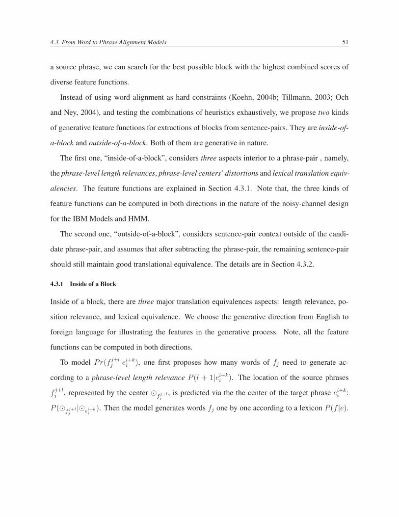
4.3. From Word to Phrase Alignment Models 51
a source phrase, we can search for the best possible block with the highest combined scores of
diverse feature functions.
Instead of using word alignment as hard constraints (Koehn, 2004b; Tillmann, 2003; Och
and Ney, 2004), and testing the combinations of heuristics exhaustively, we propose two kinds
of generative feature functions for extractions of blocks from sentence-pairs. They are inside-of-
a-block and outside-of-a-block. Both of them are generative in nature.
The first one, “inside-of-a-block”, considers three aspects interior to a phrase-pair , namely,
the phrase-level length relevances, phrase-level centers’ distortions and lexical translation equiv-
alencies. The feature functions are explained in Section 4.3.1. Note that, the three kinds of
feature functions can be computed in both directions in the nature of the noisy-channel design
for the IBM Models and HMM.
The second one, “outside-of-a-block”, considers sentence-pair context outside of the candi-
date phrase-pair, and assumes that after subtracting the phrase-pair, the remaining sentence-pair
should still maintain good translational equivalence. The details are in Section 4.3.2.
4.3.1 Inside of a Block
Inside of a block, there are three major translation equivalences aspects: length relevance, po-
sition relevance, and lexical equivalence. We choose the generative direction from English to
foreign language for illustrating the features in the generative process. Note, all the feature
functions can be computed in both directions.
To model Pr(f j+lj |ei+k
i ), one first proposes how many words of fj need to generate ac-
cording to a phrase-level length relevance P (l + 1|ei+ki ). The location of the source phrases
f j+lj , represented by the center ¯fj+l
j, is predicted via the the center of the target phrase ei+k
i :
P (¯fj+lj|¯ei+k
i). Then the model generates words fj one by one according to a lexicon P (f |e).

4.3. From Word to Phrase Alignment Models 52
This generative process is summarized in Eqn. 4.9.
Pr(f j+lj |ei+k
i ) = max{ei+k
i }P (l + 1|ei+k
i ) ·
P (¯fj+lj|¯ei+k
i) ·
P (f j+lj |ei+k
i ), (4.9)
where the three components P (l+1|ei+ki ), P (¯fj+l
j|¯ei+k
i) and P (f j+l
j |ei+ki ) control three differ-
ent aspects of a block: phrase-level fertility, center distortion and lexical translation equivalence.
A variation of this model was applied in a ACL05 shared task for phrase-based statistical ma-
chine translation in (Zhao and Vogel, 2005).
A Phrase-Level Length Model: Translation length is an important feature used by human
translator. A word in Chinese is typically translated into less than four English words; it is
very rare to see a Chinese word translated into more than eight English words. The word-
fertility defined in Brown et al. (1993) models such an assumption at word level. In this work,
we generalize the length-relevance for a block, and predict how many source words need to
generate given the length of the target phrase.
Given the candidate target phrase (English) ei+ki and a source phrase f j+l
j , this model gives
the probabilistic estimation of P (l+1|eI1), computed via a dynamic programming algorithm us-
ing the English word fertilities model P (φ|ei), where φ is number of words with typical value
from one to eight. Figure 4.4 shows an example fertility trellis for an English trigram, where
each edge between two nodes represents one English word ei. The arc between two nodes rep-
resents one candidate non-zero fertility for word ei. The fertility of zero (i.e., generating a Null
word) corresponds to the direct edge between two nodes and thus, the Null word is naturally in-
corporated into this model’s representation. Each arc is associated with an English word fertility
probability P (φi|ei). A path φi+ki through the trellis represents the number of French words φi
generated by each of the English word in the trigram. The probability of generating l + 1 words
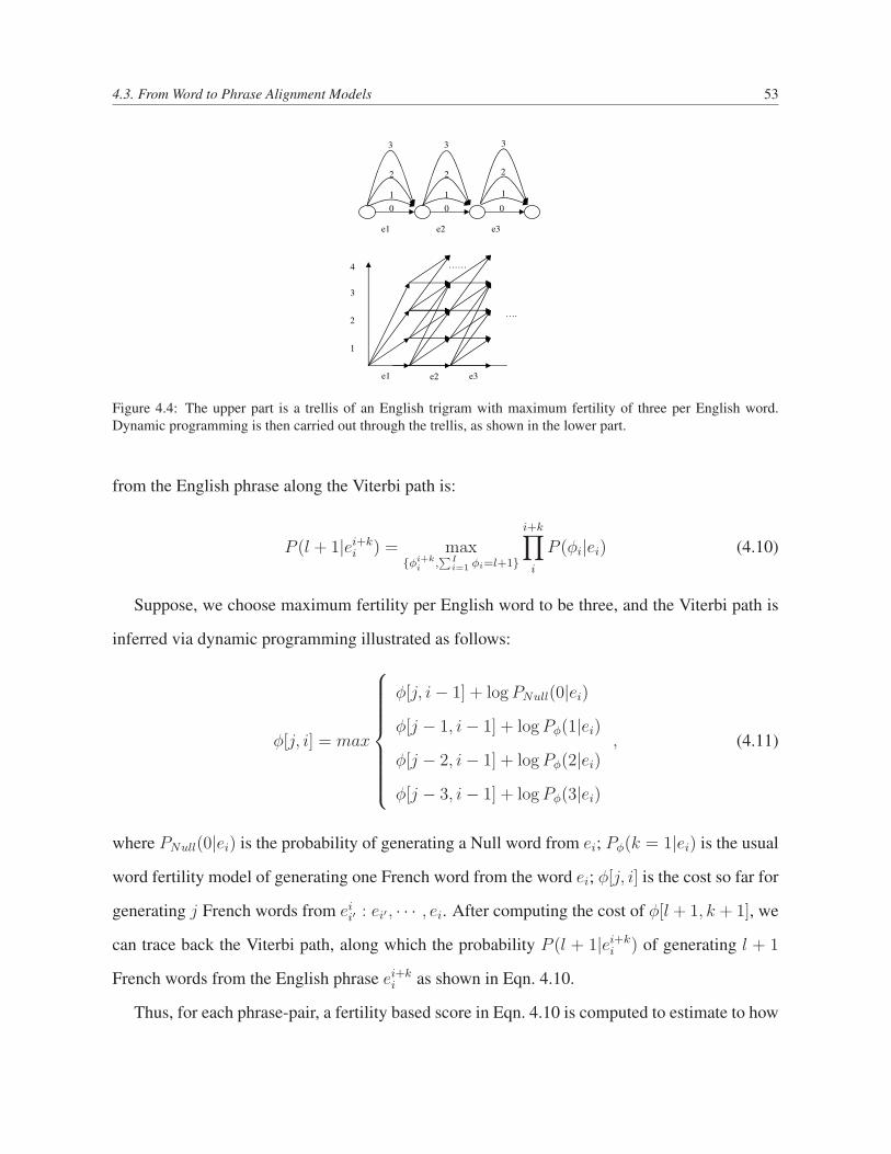
4.3. From Word to Phrase Alignment Models 53
e1 e2 e3
1
3
2
0 0
2
0
e1 e2 e3
……
….
1
2
3
4
3
1
3
1
2
Figure 4.4: The upper part is a trellis of an English trigram with maximum fertility of three per English word.Dynamic programming is then carried out through the trellis, as shown in the lower part.
from the English phrase along the Viterbi path is:
P (l + 1|ei+ki ) = max
{φi+ki ,
∑Ii=1 φi=l+1}
i+k∏i
P (φi|ei) (4.10)
Suppose, we choose maximum fertility per English word to be three, and the Viterbi path is
inferred via dynamic programming illustrated as follows:
φ[j, i] = max
φ[j, i− 1] + log PNull(0|ei)
φ[j − 1, i− 1] + log Pφ(1|ei)
φ[j − 2, i− 1] + log Pφ(2|ei)
φ[j − 3, i− 1] + log Pφ(3|ei)
, (4.11)
where PNull(0|ei) is the probability of generating a Null word from ei; Pφ(k = 1|ei) is the usual
word fertility model of generating one French word from the word ei; φ[j, i] is the cost so far for
generating j French words from eii′ : ei′ , · · · , ei. After computing the cost of φ[l + 1, k + 1], we
can trace back the Viterbi path, along which the probability P (l + 1|ei+ki ) of generating l + 1
French words from the English phrase ei+ki as shown in Eqn. 4.10.
Thus, for each phrase-pair, a fertility based score in Eqn. 4.10 is computed to estimate to how
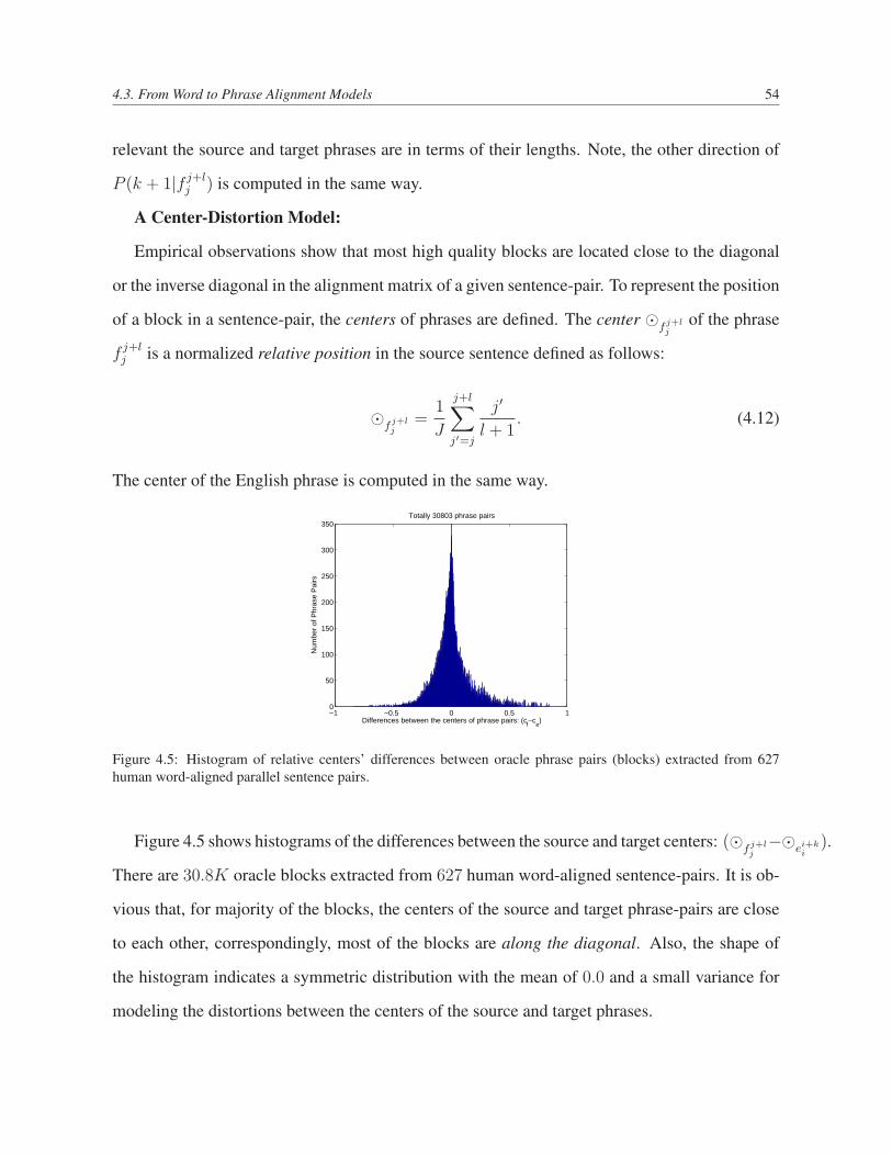
4.3. From Word to Phrase Alignment Models 54
relevant the source and target phrases are in terms of their lengths. Note, the other direction of
P (k + 1|f j+lj ) is computed in the same way.
A Center-Distortion Model:
Empirical observations show that most high quality blocks are located close to the diagonal
or the inverse diagonal in the alignment matrix of a given sentence-pair. To represent the position
of a block in a sentence-pair, the centers of phrases are defined. The center ¯fj+lj
of the phrase
f j+lj is a normalized relative position in the source sentence defined as follows:
¯fj+lj
=1
J
j+l∑
j′=j
j′
l + 1. (4.12)
The center of the English phrase is computed in the same way.
−1 −0.5 0 0.5 10
50
100
150
200
250
300
350
Num
ber
of P
hras
e P
airs
Differences between the centers of phrase pairs: (cf−c
e)
Totally 30803 phrase pairs
Figure 4.5: Histogram of relative centers’ differences between oracle phrase pairs (blocks) extracted from 627human word-aligned parallel sentence pairs.
Figure 4.5 shows histograms of the differences between the source and target centers: (¯fj+lj−¯ei+k
i).
There are 30.8K oracle blocks extracted from 627 human word-aligned sentence-pairs. It is ob-
vious that, for majority of the blocks, the centers of the source and target phrase-pairs are close
to each other, correspondingly, most of the blocks are along the diagonal. Also, the shape of
the histogram indicates a symmetric distribution with the mean of 0.0 and a small variance for
modeling the distortions between the centers of the source and target phrases.
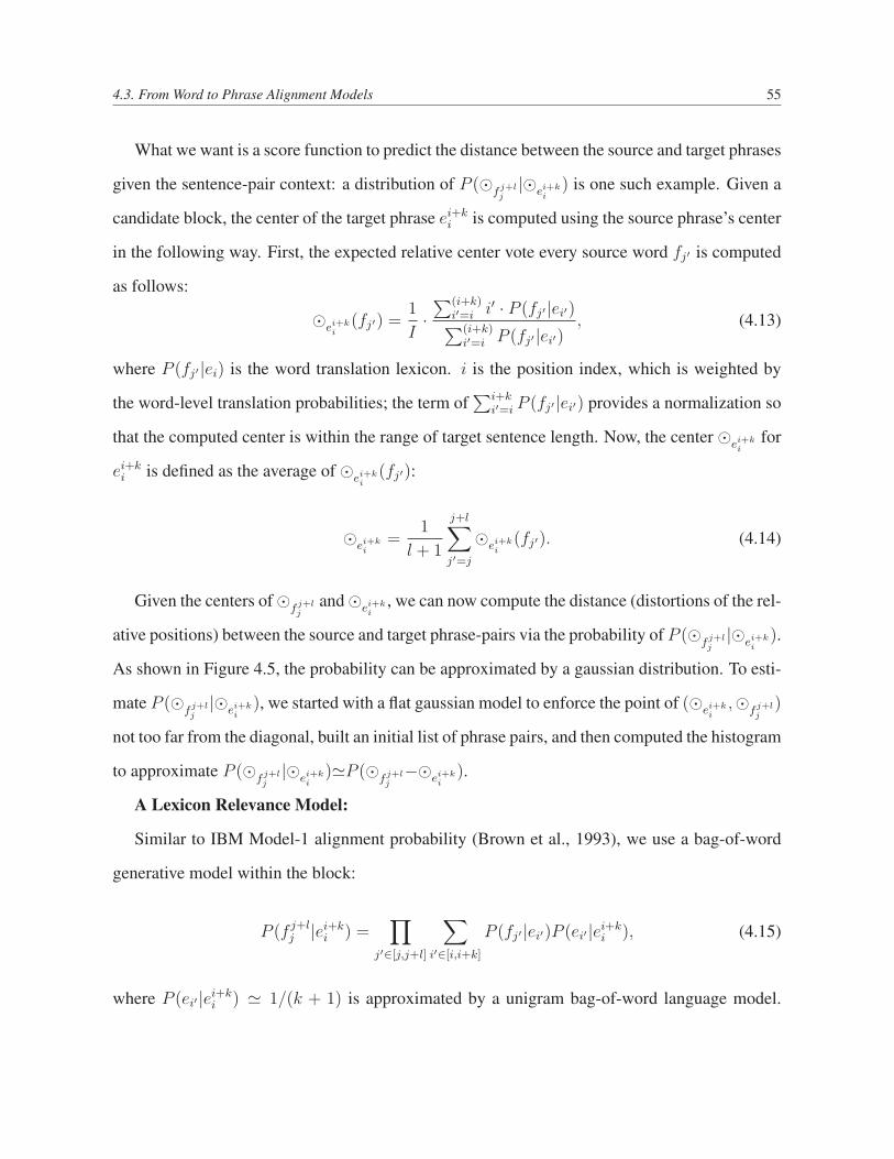
4.3. From Word to Phrase Alignment Models 55
What we want is a score function to predict the distance between the source and target phrases
given the sentence-pair context: a distribution of P (¯fj+lj|¯ei+k
i) is one such example. Given a
candidate block, the center of the target phrase ei+ki is computed using the source phrase’s center
in the following way. First, the expected relative center vote every source word fj′ is computed
as follows:
¯ei+ki
(fj′) =1
I·∑(i+k)
i′=i i′ · P (fj′|ei′)∑(i+k)i′=i P (fj′|ei′)
, (4.13)
where P (fj′|ei) is the word translation lexicon. i is the position index, which is weighted by
the word-level translation probabilities; the term of∑i+k
i′=i P (fj′|ei′) provides a normalization so
that the computed center is within the range of target sentence length. Now, the center ¯ei+ki
for
ei+ki is defined as the average of ¯ei+k
i(fj′):
¯ei+ki
=1
l + 1
j+l∑
j′=j
¯ei+ki
(fj′). (4.14)
Given the centers of¯fj+lj
and¯ei+ki
, we can now compute the distance (distortions of the rel-
ative positions) between the source and target phrase-pairs via the probability of P (¯fj+lj|¯ei+k
i).
As shown in Figure 4.5, the probability can be approximated by a gaussian distribution. To esti-
mate P (¯fj+lj|¯ei+k
i), we started with a flat gaussian model to enforce the point of (¯ei+k
i,¯fj+l
j)
not too far from the diagonal, built an initial list of phrase pairs, and then computed the histogram
to approximate P (¯fj+lj|¯ei+k
i)'P (¯fj+l
j−¯ei+k
i).
A Lexicon Relevance Model:
Similar to IBM Model-1 alignment probability (Brown et al., 1993), we use a bag-of-word
generative model within the block:
P (f j+lj |ei+k
i ) =∏
j′∈[j,j+l]
∑
i′∈[i,i+k]
P (fj′|ei′)P (ei′|ei+ki ), (4.15)
where P (ei′|ei+ki ) ' 1/(k + 1) is approximated by a unigram bag-of-word language model.
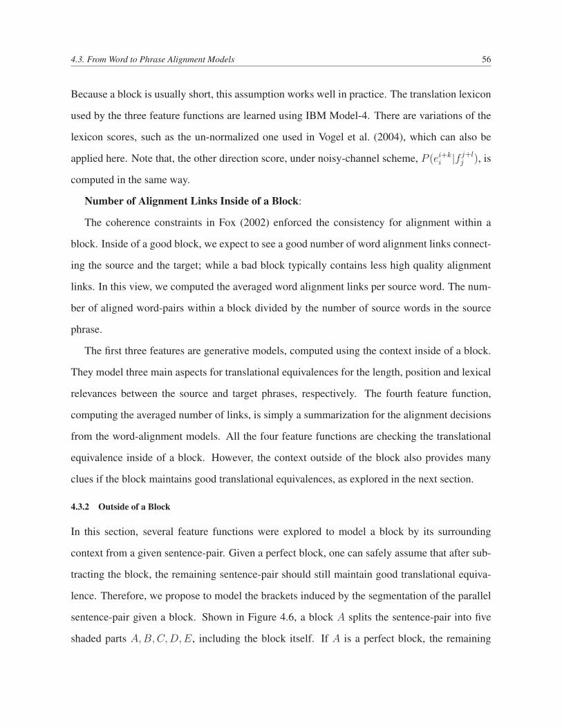
4.3. From Word to Phrase Alignment Models 56
Because a block is usually short, this assumption works well in practice. The translation lexicon
used by the three feature functions are learned using IBM Model-4. There are variations of the
lexicon scores, such as the un-normalized one used in Vogel et al. (2004), which can also be
applied here. Note that, the other direction score, under noisy-channel scheme, P (ei+ki |f j+l
j ), is
computed in the same way.
Number of Alignment Links Inside of a Block:
The coherence constraints in Fox (2002) enforced the consistency for alignment within a
block. Inside of a good block, we expect to see a good number of word alignment links connect-
ing the source and the target; while a bad block typically contains less high quality alignment
links. In this view, we computed the averaged word alignment links per source word. The num-
ber of aligned word-pairs within a block divided by the number of source words in the source
phrase.
The first three features are generative models, computed using the context inside of a block.
They model three main aspects for translational equivalences for the length, position and lexical
relevances between the source and target phrases, respectively. The fourth feature function,
computing the averaged number of links, is simply a summarization for the alignment decisions
from the word-alignment models. All the four feature functions are checking the translational
equivalence inside of a block. However, the context outside of the block also provides many
clues if the block maintains good translational equivalences, as explored in the next section.
4.3.2 Outside of a Block
In this section, several feature functions were explored to model a block by its surrounding
context from a given sentence-pair. Given a perfect block, one can safely assume that after sub-
tracting the block, the remaining sentence-pair should still maintain good translational equiva-
lence. Therefore, we propose to model the brackets induced by the segmentation of the parallel
sentence-pair given a block. Shown in Figure 4.6, a block A splits the sentence-pair into five
shaded parts A,B,C,D,E, including the block itself. If A is a perfect block, the remaining
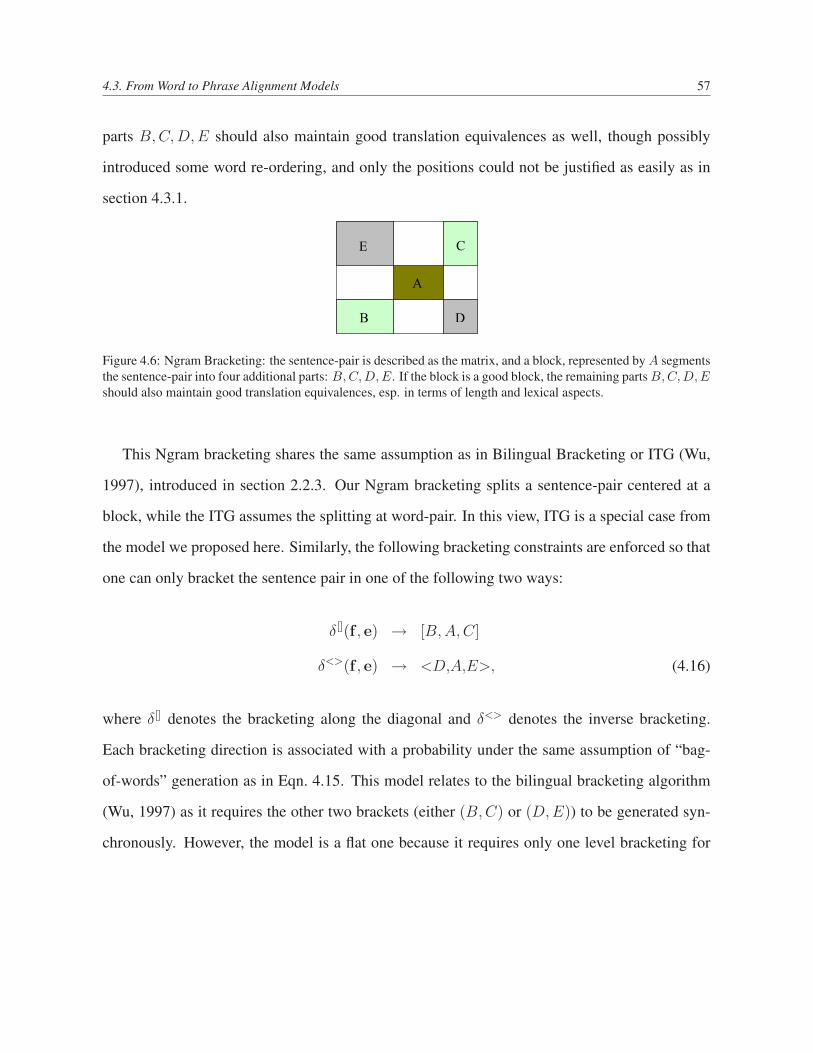
4.3. From Word to Phrase Alignment Models 57
parts B, C, D, E should also maintain good translation equivalences as well, though possibly
introduced some word re-ordering, and only the positions could not be justified as easily as in
section 4.3.1.
A
C
B D
E
Figure 4.6: Ngram Bracketing: the sentence-pair is described as the matrix, and a block, represented by A segmentsthe sentence-pair into four additional parts: B,C, D,E. If the block is a good block, the remaining parts B,C, D,Eshould also maintain good translation equivalences, esp. in terms of length and lexical aspects.
This Ngram bracketing shares the same assumption as in Bilingual Bracketing or ITG (Wu,
1997), introduced in section 2.2.3. Our Ngram bracketing splits a sentence-pair centered at a
block, while the ITG assumes the splitting at word-pair. In this view, ITG is a special case from
the model we proposed here. Similarly, the following bracketing constraints are enforced so that
one can only bracket the sentence pair in one of the following two ways:
δ[](f , e) → [B, A,C]
δ<>(f , e) → <D,A,E>, (4.16)
where δ[] denotes the bracketing along the diagonal and δ<> denotes the inverse bracketing.
Each bracketing direction is associated with a probability under the same assumption of “bag-
of-words” generation as in Eqn. 4.15. This model relates to the bilingual bracketing algorithm
(Wu, 1997) as it requires the other two brackets (either (B, C) or (D,E)) to be generated syn-
chronously. However, the model is a flat one because it requires only one level bracketing for
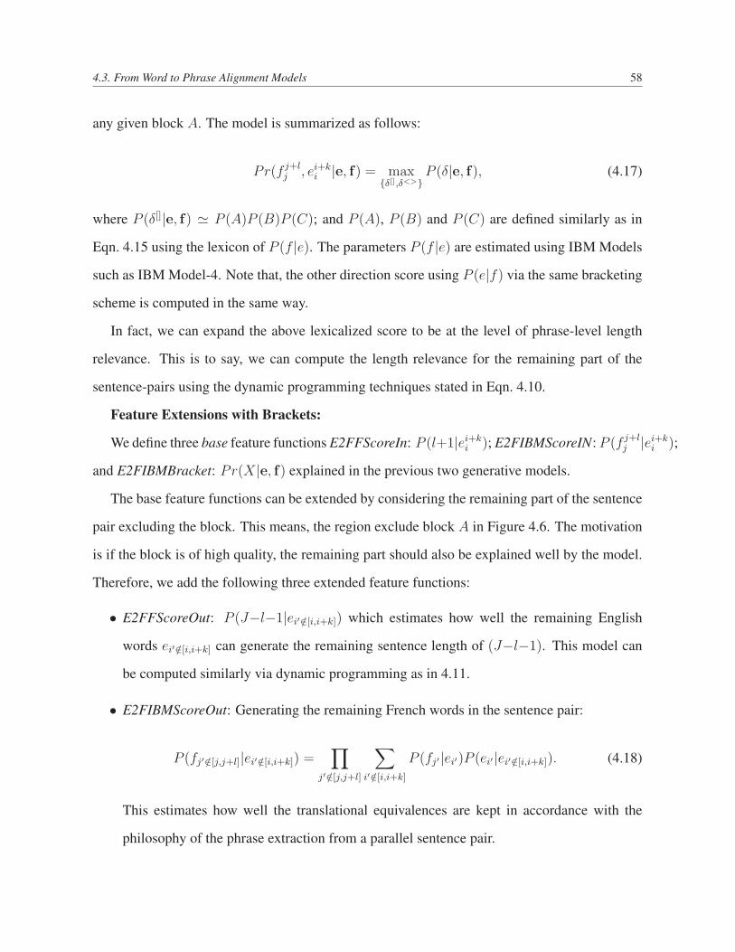
4.3. From Word to Phrase Alignment Models 58
any given block A. The model is summarized as follows:
Pr(f j+lj , ei+k
i |e, f) = max{δ[],δ<>}
P (δ|e, f), (4.17)
where P (δ[]|e, f) ' P (A)P (B)P (C); and P (A), P (B) and P (C) are defined similarly as in
Eqn. 4.15 using the lexicon of P (f |e). The parameters P (f |e) are estimated using IBM Models
such as IBM Model-4. Note that, the other direction score using P (e|f) via the same bracketing
scheme is computed in the same way.
In fact, we can expand the above lexicalized score to be at the level of phrase-level length
relevance. This is to say, we can compute the length relevance for the remaining part of the
sentence-pairs using the dynamic programming techniques stated in Eqn. 4.10.
Feature Extensions with Brackets:
We define three base feature functions E2FFScoreIn: P (l+1|ei+ki ); E2FIBMScoreIN: P (f j+l
j |ei+ki );
and E2FIBMBracket: Pr(X|e, f) explained in the previous two generative models.
The base feature functions can be extended by considering the remaining part of the sentence
pair excluding the block. This means, the region exclude block A in Figure 4.6. The motivation
is if the block is of high quality, the remaining part should also be explained well by the model.
Therefore, we add the following three extended feature functions:
• E2FFScoreOut: P (J−l−1|ei′ /∈[i,i+k]) which estimates how well the remaining English
words ei′ /∈[i,i+k] can generate the remaining sentence length of (J−l−1). This model can
be computed similarly via dynamic programming as in 4.11.
• E2FIBMScoreOut: Generating the remaining French words in the sentence pair:
P (fj′ /∈[j,j+l]|ei′ /∈[i,i+k]) =∏
j′ /∈[j,j+l]
∑
i′ /∈[i,i+k]
P (fj′|ei′)P (ei′|ei′ /∈[i,i+k]). (4.18)
This estimates how well the translational equivalences are kept in accordance with the
philosophy of the phrase extraction from a parallel sentence pair.
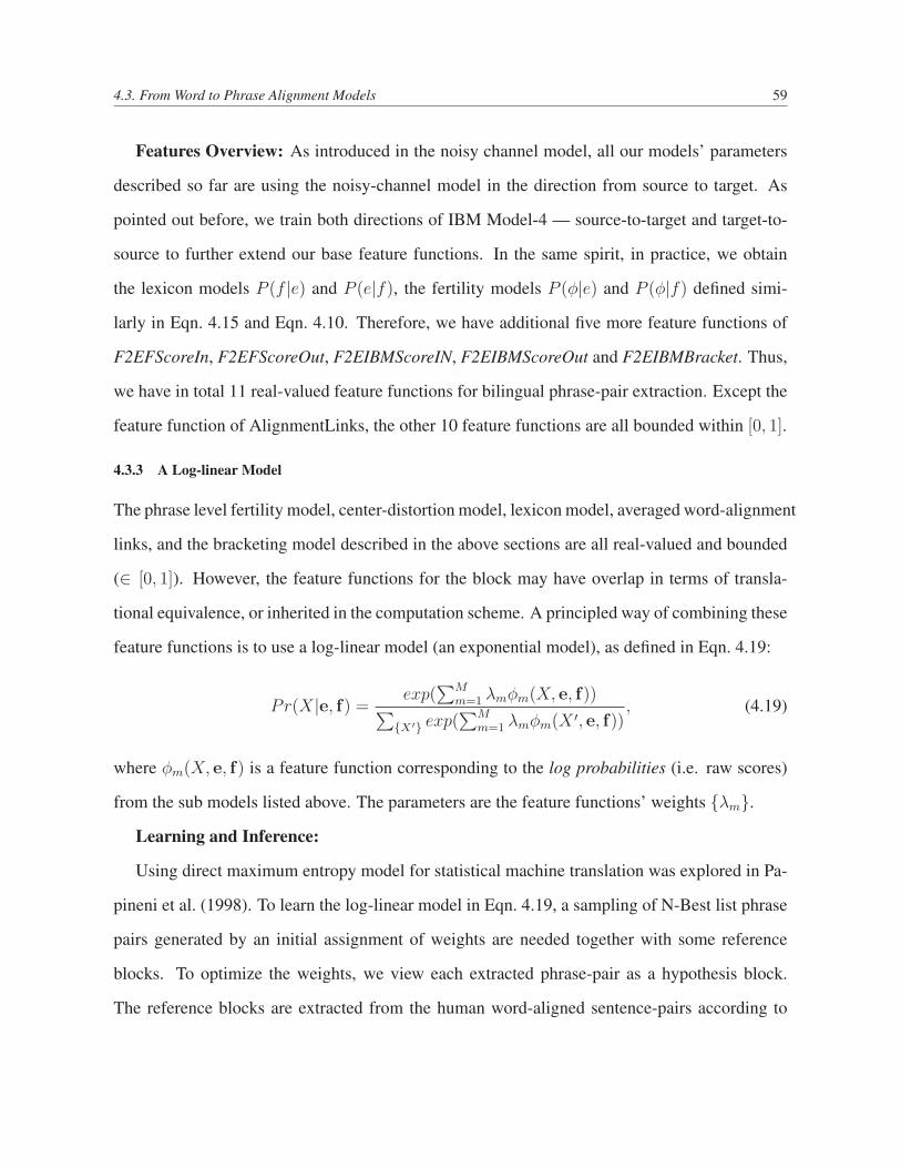
4.3. From Word to Phrase Alignment Models 59
Features Overview: As introduced in the noisy channel model, all our models’ parameters
described so far are using the noisy-channel model in the direction from source to target. As
pointed out before, we train both directions of IBM Model-4 — source-to-target and target-to-
source to further extend our base feature functions. In the same spirit, in practice, we obtain
the lexicon models P (f |e) and P (e|f), the fertility models P (φ|e) and P (φ|f) defined simi-
larly in Eqn. 4.15 and Eqn. 4.10. Therefore, we have additional five more feature functions of
F2EFScoreIn, F2EFScoreOut, F2EIBMScoreIN, F2EIBMScoreOut and F2EIBMBracket. Thus,
we have in total 11 real-valued feature functions for bilingual phrase-pair extraction. Except the
feature function of AlignmentLinks, the other 10 feature functions are all bounded within [0, 1].
4.3.3 A Log-linear Model
The phrase level fertility model, center-distortion model, lexicon model, averaged word-alignment
links, and the bracketing model described in the above sections are all real-valued and bounded
(∈ [0, 1]). However, the feature functions for the block may have overlap in terms of transla-
tional equivalence, or inherited in the computation scheme. A principled way of combining these
feature functions is to use a log-linear model (an exponential model), as defined in Eqn. 4.19:
Pr(X|e, f) =exp(
∑Mm=1 λmφm(X, e, f))∑
{X′} exp(∑M
m=1 λmφm(X ′, e, f)), (4.19)
where φm(X, e, f) is a feature function corresponding to the log probabilities (i.e. raw scores)
from the sub models listed above. The parameters are the feature functions’ weights {λm}.
Learning and Inference:
Using direct maximum entropy model for statistical machine translation was explored in Pa-
pineni et al. (1998). To learn the log-linear model in Eqn. 4.19, a sampling of N-Best list phrase
pairs generated by an initial assignment of weights are needed together with some reference
blocks. To optimize the weights, we view each extracted phrase-pair as a hypothesis block.
The reference blocks are extracted from the human word-aligned sentence-pairs according to

4.4. Experiments 60
the “coherence” constraints proposed by Fox (2002). We compute word-level F-measure for
each extracted block according to all the reference blocks, which contain the same extracted
source phrase. Therefore, the data point for optimization is M raw scores 2 of feature functions
together with a performance indicator of word-level F-measure. Finally, an optimizer similar to
Och and Ney (2002) can be utilized to ofbtain the optimized weights for the proposed feature
functions. Other optimization methods including generalized downhill simplex (in particular,
see http://paula.univ.gda.pl/ dokgrk/simplex.html) are also effective in practice.
The inference is a hill-climbing with a performance measure to score the phrase pairs (f j+lj , ei+k
i )
according to the log-linear model as in Eqn 4.20:
X = arg max{X}
M∑m=1
λmφm(X, e, f), (4.20)
where φm(X, e, f) are log probabilities computed using the models and their extensions dis-
cussed in section 4.3.3.
4.4 Experiments
4.4.1 Extended HMM with Bilingual Word Clusters
In the experiments for word clusters, we applied it to the TIDES Chinese-English small data
track evaluation test set. After preprocessing, including English tokenization, Chinese word
segmentation, and parallel sentence splitting, there are in total 4172 parallel sentence pairs for
training. We manually labeled word alignments for 627 test sentence pairs randomly sampled
from the dry-run test data in 2001, which has four human reference translations for each Chinese
sentence. The preprocessing for the test data was different from the above, as it was designed
for humans to label word alignments correctly by removing ambiguities from tokenization and
word segmentation as much as possible. The data statistics are shown in Table 1.2The log probabilities from sub-models; in our case M=11
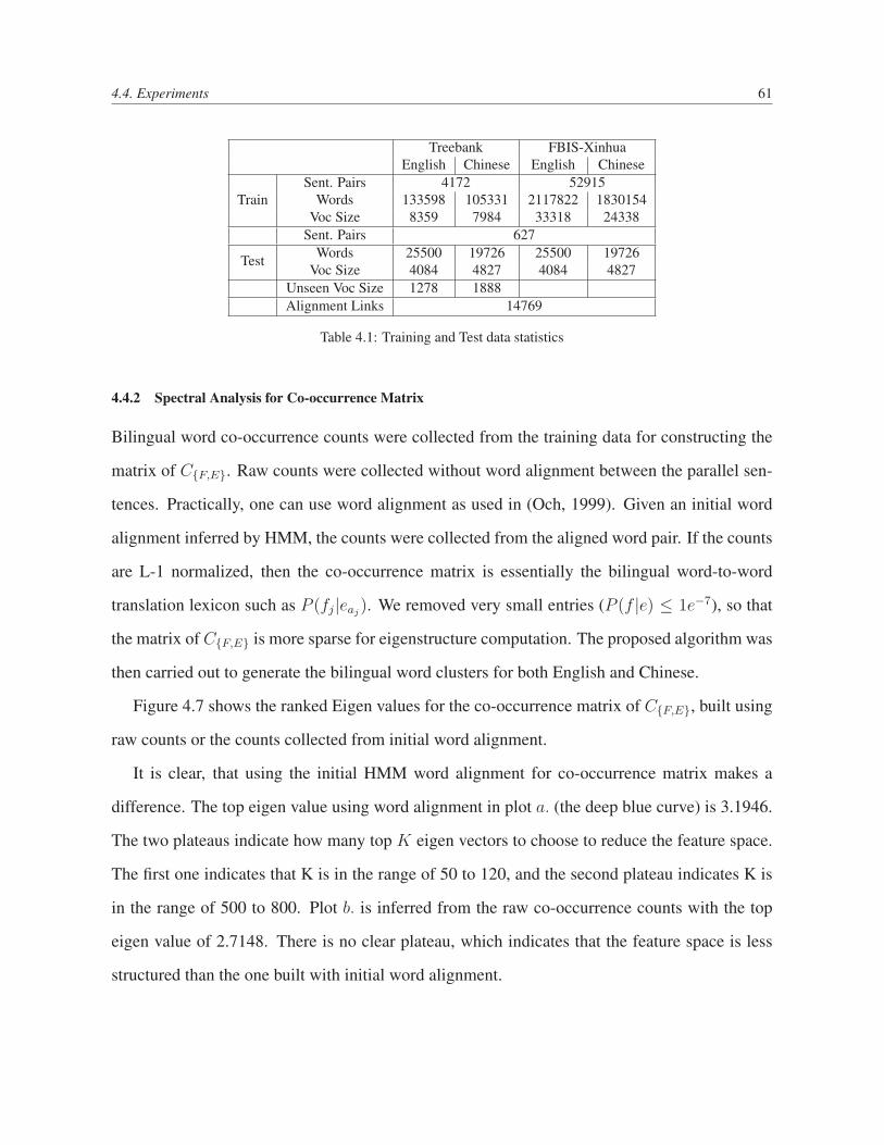
4.4. Experiments 61
Treebank FBIS-XinhuaEnglish Chinese English Chinese
TrainSent. Pairs 4172 52915
Words 133598 105331 2117822 1830154Voc Size 8359 7984 33318 24338
Test
Sent. Pairs 627Words 25500 19726 25500 19726
Voc Size 4084 4827 4084 4827Unseen Voc Size 1278 1888Alignment Links 14769
Table 4.1: Training and Test data statistics
4.4.2 Spectral Analysis for Co-occurrence Matrix
Bilingual word co-occurrence counts were collected from the training data for constructing the
matrix of C{F,E}. Raw counts were collected without word alignment between the parallel sen-
tences. Practically, one can use word alignment as used in (Och, 1999). Given an initial word
alignment inferred by HMM, the counts were collected from the aligned word pair. If the counts
are L-1 normalized, then the co-occurrence matrix is essentially the bilingual word-to-word
translation lexicon such as P (fj|eaj). We removed very small entries (P (f |e) ≤ 1e−7), so that
the matrix of C{F,E} is more sparse for eigenstructure computation. The proposed algorithm was
then carried out to generate the bilingual word clusters for both English and Chinese.
Figure 4.7 shows the ranked Eigen values for the co-occurrence matrix of C{F,E}, built using
raw counts or the counts collected from initial word alignment.
It is clear, that using the initial HMM word alignment for co-occurrence matrix makes a
difference. The top eigen value using word alignment in plot a. (the deep blue curve) is 3.1946.
The two plateaus indicate how many top K eigen vectors to choose to reduce the feature space.
The first one indicates that K is in the range of 50 to 120, and the second plateau indicates K is
in the range of 500 to 800. Plot b. is inferred from the raw co-occurrence counts with the top
eigen value of 2.7148. There is no clear plateau, which indicates that the feature space is less
structured than the one built with initial word alignment.

4.4. Experiments 62
0 100 200 300 400 500 600 700 800 900 10000.5
1
1.5
2
2.5
3
3.5Eigen values of affinity matrices
Top 1000 Eigen Values
Eig
en V
alue
s
(a) co−occur counts from init word alignment(b) raw co−occur counts from data
Figure 4.7: Top-1000 Eigen Values of Co-occurrence Matrix
We found, in our experiments, 500 top eigen vectors are good enough for bilingual clustering
in terms of efficiency and effectiveness.
4.4.3 Bilingual Spectral Clustering Results
Clusters built via the two described methods are compared. The first method bil1 is the two-step
optimization approach: first optimizing the monolingual clusters for target language (English),
and afterwards optimizing clusters for the source language (Chinese). The second method bil2 is
our proposed algorithm to compute the eigenstructure of the co-occurrence matrix, which builds
the left and right subspaces, and finds clusters in such spaces. Top 500 eigen vectors were used
to construct these subspaces. For both methods, 1000 clusters were inferred for English and
Chinese respectively. The number of clusters is chosen in a way that the final word alignment
accuracy was optimal. Table 4.2 provides the clustering examples using the two algorithms.
The monolingual word clusters often contain words with similar syntax functions. This hap-
pens with esp. frequent words (eg. mono-E1 and mono-E2). The algorithm tends to put rare
words such as “carota, anglophobia” into a very big cluster (eg. mono-E3). In addition, the
words within these monolingual clusters rarely share similar translations such as the typical
cluster of “week, month, year”. This indicates that the corresponding Chinese clusters inferred
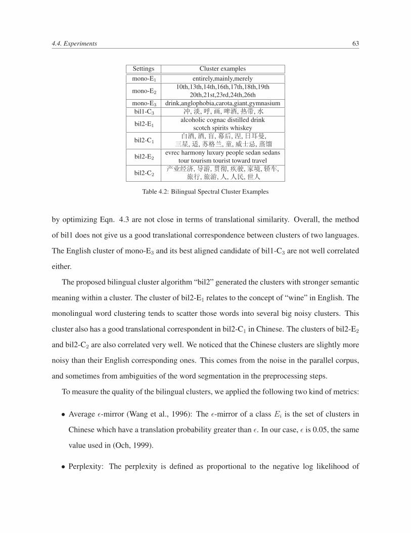
4.4. Experiments 63
Settings Cluster examplesmono-E1 entirely,mainly,merely
mono-E210th,13th,14th,16th,17th,18th,19th
20th,21st,23rd,24th,26thmono-E3 drink,anglophobia,carota,giant,gymnasiumbil1-C3 冲,淡,呼,画,啤酒,热带,水
bil2-E1alcoholic cognac distilled drink
scotch spirits whiskey
bil2-C1白酒,酒,盲,幕后,涅,日耳曼,三星,适,苏格兰,童,威士忌,蒸馏
bil2-E2evrec harmony luxury people sedan sedans
tour tourism tourist toward travel
bil2-C2产业经济,导游,贯彻,疾驶,家境,轿车,
旅行,旅游,人,人民,世人
Table 4.2: Bilingual Spectral Cluster Examples
by optimizing Eqn. 4.3 are not close in terms of translational similarity. Overall, the method
of bil1 does not give us a good translational correspondence between clusters of two languages.
The English cluster of mono-E3 and its best aligned candidate of bil1-C3 are not well correlated
either.
The proposed bilingual cluster algorithm “bil2” generated the clusters with stronger semantic
meaning within a cluster. The cluster of bil2-E1 relates to the concept of “wine” in English. The
monolingual word clustering tends to scatter those words into several big noisy clusters. This
cluster also has a good translational correspondent in bil2-C1 in Chinese. The clusters of bil2-E2
and bil2-C2 are also correlated very well. We noticed that the Chinese clusters are slightly more
noisy than their English corresponding ones. This comes from the noise in the parallel corpus,
and sometimes from ambiguities of the word segmentation in the preprocessing steps.
To measure the quality of the bilingual clusters, we applied the following two kind of metrics:
• Average ε-mirror (Wang et al., 1996): The ε-mirror of a class Ei is the set of clusters in
Chinese which have a translation probability greater than ε. In our case, ε is 0.05, the same
value used in (Och, 1999).
• Perplexity: The perplexity is defined as proportional to the negative log likelihood of
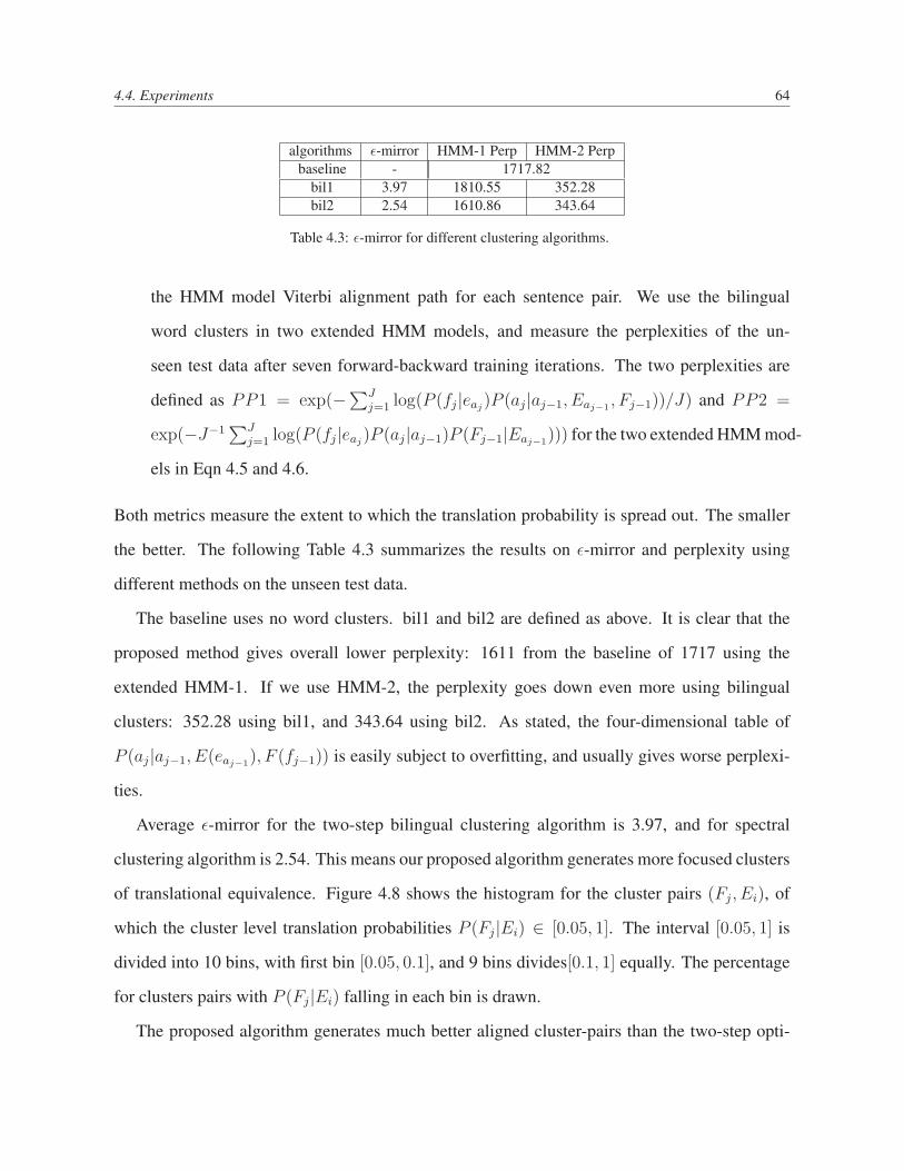
4.4. Experiments 64
algorithms ε-mirror HMM-1 Perp HMM-2 Perpbaseline - 1717.82
bil1 3.97 1810.55 352.28bil2 2.54 1610.86 343.64
Table 4.3: ε-mirror for different clustering algorithms.
the HMM model Viterbi alignment path for each sentence pair. We use the bilingual
word clusters in two extended HMM models, and measure the perplexities of the un-
seen test data after seven forward-backward training iterations. The two perplexities are
defined as PP1 = exp(−∑Jj=1 log(P (fj|eaj
)P (aj|aj−1, Eaj−1, Fj−1))/J) and PP2 =
exp(−J−1∑J
j=1 log(P (fj|eaj)P (aj|aj−1)P (Fj−1|Eaj−1
))) for the two extended HMM mod-
els in Eqn 4.5 and 4.6.
Both metrics measure the extent to which the translation probability is spread out. The smaller
the better. The following Table 4.3 summarizes the results on ε-mirror and perplexity using
different methods on the unseen test data.
The baseline uses no word clusters. bil1 and bil2 are defined as above. It is clear that the
proposed method gives overall lower perplexity: 1611 from the baseline of 1717 using the
extended HMM-1. If we use HMM-2, the perplexity goes down even more using bilingual
clusters: 352.28 using bil1, and 343.64 using bil2. As stated, the four-dimensional table of
P (aj|aj−1, E(eaj−1), F (fj−1)) is easily subject to overfitting, and usually gives worse perplexi-
ties.
Average ε-mirror for the two-step bilingual clustering algorithm is 3.97, and for spectral
clustering algorithm is 2.54. This means our proposed algorithm generates more focused clusters
of translational equivalence. Figure 4.8 shows the histogram for the cluster pairs (Fj, Ei), of
which the cluster level translation probabilities P (Fj|Ei) ∈ [0.05, 1]. The interval [0.05, 1] is
divided into 10 bins, with first bin [0.05, 0.1], and 9 bins divides[0.1, 1] equally. The percentage
for clusters pairs with P (Fj|Ei) falling in each bin is drawn.
The proposed algorithm generates much better aligned cluster-pairs than the two-step opti-
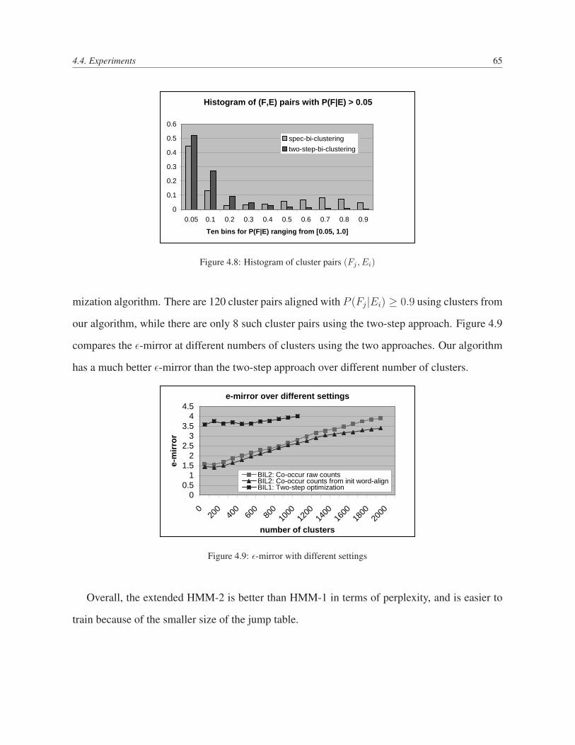
4.4. Experiments 65
Histogram of (F,E) pairs with P(F|E) > 0.05
0
0.1
0.2
0.3
0.4
0.5
0.6
0.05 0.1 0.2 0.3 0.4 0.5 0.6 0.7 0.8 0.9
Ten bins for P(F|E) ranging from [0.05, 1.0]
spec-bi-clustering
two-step-bi-clustering
Figure 4.8: Histogram of cluster pairs (Fj , Ei)
mization algorithm. There are 120 cluster pairs aligned with P (Fj|Ei) ≥ 0.9 using clusters from
our algorithm, while there are only 8 such cluster pairs using the two-step approach. Figure 4.9
compares the ε-mirror at different numbers of clusters using the two approaches. Our algorithm
has a much better ε-mirror than the two-step approach over different number of clusters.
e-mirror over different settings
00.5
11.5
22.5
33.5
44.5
020
040
060
080
010
0012
0014
0016
0018
0020
00
number of clusters
e-m
irro
r
BIL2: Co-occur raw countsBIL2: Co-occur counts from init word-alignBIL1: Two-step optimization
Figure 4.9: ε-mirror with different settings
Overall, the extended HMM-2 is better than HMM-1 in terms of perplexity, and is easier to
train because of the smaller size of the jump table.
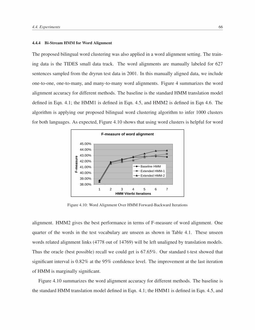
4.4. Experiments 66
4.4.4 Bi-Stream HMM for Word Alignment
The proposed bilingual word clustering was also applied in a word alignment setting. The train-
ing data is the TIDES small data track. The word alignments are manually labeled for 627
sentences sampled from the dryrun test data in 2001. In this manually aligned data, we include
one-to-one, one-to-many, and many-to-many word alignments. Figure 4 summarizes the word
alignment accuracy for different methods. The baseline is the standard HMM translation model
defined in Eqn. 4.1; the HMM1 is defined in Eqn. 4.5, and HMM2 is defined in Eqn 4.6. The
algorithm is applying our proposed bilingual word clustering algorithm to infer 1000 clusters
for both languages. As expected, Figure 4.10 shows that using word clusters is helpful for word
F-measure of word alignment
38.00%
39.00%
40.00%
41.00%
42.00%
43.00%
44.00%
45.00%
1 2 3 4 5 6 7HMM Viterbi Iterations
F-m
easu
re
Baseline HMM
Extended HMM-1
Extended HMM-2
Figure 4.10: Word Alignment Over HMM Forward-Backward Iterations
alignment. HMM2 gives the best performance in terms of F-measure of word alignment. One
quarter of the words in the test vocabulary are unseen as shown in Table 4.1. These unseen
words related alignment links (4778 out of 14769) will be left unaligned by translation models.
Thus the oracle (best possible) recall we could get is 67.65%. Our standard t-test showed that
significant interval is 0.82% at the 95% confidence level. The improvement at the last iteration
of HMM is marginally significant.
Figure 4.10 summarizes the word alignment accuracy for different methods. The baseline is
the standard HMM translation model defined in Eqn. 4.1; the HMM1 is defined in Eqn. 4.5, and
4.4. Experiments 67
HMM2 is defined in Eqn 4.6. The algorithm is applying our proposed bilingual word clustering
algorithm to infer 1000 clusters for both languages. Figure 4.10 shows that using word clusters
is helpful for word alignment. HMM2 gives the best performance in terms of F-measure of word
alignment. HMM1 is susceptible to data sparseness, but it still outperforms the baseline HMM.
In the later experiments, we only show the results using HMM2, which is Bi-Stream HMM using
the Bilingual Word Spectrum Clusters.
4.4.5 Comparing with Symmetrized Word Alignments from IBM Model 4
In this experiment, all the parameters for training extended Bi-Stream HMMs and IBM Model-4
were tuned for the optimal performance for word alignment accuracy. Refined word alignments
from directions of Chinese-to-English and English-to-Chinese are also collected for compar-
isons. The NULL word alignment is specially treated in Bi-Stream HMM in GIZA++. There-
fore, we tuned the smoothing for NULL word to be optimal for all the Bi-Stream HMM and
IBM Model-4.
We collected 50 monolingual word clusters, and the 1000 word clusters inferred by spectral
clustering. Translation models were trained using the scheme of 15h53243, in which HMM
is the version of extended HMM-2 (Bi-Stream HMM); IBM Model-4 is the standard one in
GIZA++ without the cluster information. Two iterations of Model-3 seem to help slightly in our
experiments for the treebank data.
The results shown in Table 4.4 provide several interesting observations. First, the direction
of English-to-Chinese word alignment performance is usually better than the other direction.
Second, extended HMMs with bilingual word clusters are usually better than the monolingual
word clusters. Third, extended HMMs are usually better than IBM Model-4. There could be two
reasons: there is no word clusters information in IBM Model-4; IBM Model-4 may suffer from
data sparseness from this small training data and the FBIS data. However, our later experiments
show that even using decent amount of training data (about 2 million words on the source side),
the extended HMM still outperform the IBM Model-4.

4.4. Experiments 68
Treebank Data Bi-Stream HMM IBM Model-4Settings Precision (%) Recall (%) F-measure (%) Precision (%) Recall (%) F-measure (%)base-ef 38.87 54.95 45.53 35.09 56.45 43.28base-fe 40.31 50.17 44.70 38.11 48.68 42.75base-refined 36.30 66.42 46.94 32.85 65.37 43.73m50-ef 46.77 54.42 50.30 41.08 59.02 48.44m50-fe 45.02 50.10 47.42 42.36 52.79 47.01m50-refined 62.22 41.15 49.54 55.62 45.50 50.05b1k-ef 50.42 55.87 53.00 42.12 60.45 49.65b1k-fe 50.32 51.09 50.70 45.17 54.55 49.42b1k-refined 47.08 63.48 54.07 38.83 66.88 49.13b1k-inter 69.07 40.18 50.80 63.23 44.21 52.03
Table 4.4: Word Alignment Performances for Different Models. Base: baseline system using HMM without wordclusters; ef: translating English into Chinese; m50: using 50 monolingual word non-overlapping clusters for bothlanguages in extended HMM in Eqn. 4.6; b1k: using 1000 bilingual spectral clusters for both languages in Eqn. 4.6.
FBIS Xinhua Bi-Stream HMM IBM Model-4Settings Precision (%) Recall (%) F-measure (%) Precision (%) Recall (%) F-measure (%)base-ef 43.15 58.33 49.60 40.69 65.29 50.14base-fe 43.27 54.17 48.11 45.01 57.56 50.51base-refined 59.63 43.98 50.62 57.04 51.07 53.89m50-ef 54.15 60.65 57.22 44.56 67.43 53.66m50-fe 50.29 54.27 52.20 47.91 59.96 53.26m50-refined 68.49 46.20 55.18 58.34 54.22 56.21b1k-ef 56.96 59.91 58.40 43.68 67.36 53.00b1k-fe 51.14 54.53 52.78 44.71 56.96 50.09b1k-refined 65.59 45.91 54.01 57.46 53.31 55.31b1k-inter 70.57 42.51 53.06 63.28 49.23 55.38
Table 4.5: Using FBIS data; Word Alignment Performances for Different Models. Base: baseline system usingHMM without any clusters; ef: translating English into Chinese; m50: using 50 monolingual word non-overlappingclusters for both languages in extended HMM in Eqn. 4.6; b1k: using 1000 bilingual spectral clusters for bothlanguages in Eqn. 4.6.
4.4.6 Evaluations of Log-Linear Phrase Alignment Models
To investigate the feature streams designed in section 4.3, we first analyzed the correlations
among the feature streams, and then the log-linear alignment model was applied and evalu-
ated using TIDES03 small-data track for Chinese-English. It was further tested for four dif-
ferent language-pairs in the supplied data tracks in IWSLT05: Chinese-English, Arabic-English,
Japanese-English, and Korean-English. We also applied the log-linear model of block-extraction

4.4. Experiments 69
in the evaluations of GALE 2007, for both text and ASR input, using large scale training data.
Pair-wise Correlations among Feature Functions:
The pair-wise correlations among the eleven (M=11) real-valued feature functions were in-
vestigated. The M×M correlation matrix was obtained by computing the pairwise linear corre-
lation coefficient between the feature functions. After this, the feature functions which are highly
correlated were regrouped close to each other via the standard K-means algorithm. The result is
shown in Figure 4.12, in which the color is an indicator of the correlation strength between the
two features. The feature IDs and the clusters are shown in the Table 4.11 on the left panel.
Feature Func. FID Feature Func. FIDE2FFScoreIn 2 E2FIBMBracket 9E2FIBMScoreIN 7 AlignmentLinks 11F2EIBMScoreOut 6F2EFScoreIn 1 E2FIBMScoreOut 8F2EIBMScoreIN 5 F2EIBMBracket 10E2FFScoreOut 4F2EFScoreOut 3
Figure 4.11: Clustered Feature Functions with Feature ID(FID). Each rectangle in the table corresponds to one ofthe four clusters inferred from the standard K-means algo-rithm. This clustering is based on all the blocks extractedfrom the training data; each block is associated with a 11-dimension vector, corresponding to 11 feature functions.
4
2
9
7
11
6
8
5
10
1
3
Scale Gives Value of R for Each Feature Function Pair
Feture Functions Correlations, Regrouped by Similarity via K−means
4 2 9 7 11 6 8 5 10 1 3
−1
−0.8
−0.6
−0.4
−0.2
0
0.2
0.4
0.6
0.8
1
Figure 4.12: Pair-wise correlations among 11 fea-ture functions; The color of each cell indicates thecorrelation strength between two features.
Evaluating Log Linear Model for Small-data and Large-data track in TIDES:
Table 4.6 summarizes the log-linear model’s performances at different configurations. The
CMU-SMT decoder is configured as a monotone decoding. The best BLEU for the log-linear
model is 18.34, an improvement of 1.1 BLEU points over the best baseline models’ performance
of 17.26 using the best generative model components. Table 4.7 showed the combined effects of
log-linear model and the Bi-Stream HMM, using STTK decoder, on TIDES-MT03 data.
The log-linear model has several advantages over each of the underlying generative models.
It introduces less data fragmentation, requiring fewer independence assumptions, and exploiting
a principled technique for automatic feature weighting. However, a drawback in our approach is
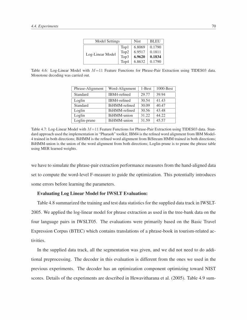
4.4. Experiments 70
Model Settings Nist BLEU
Log-Linear Model
Top1 6.8069 0.1790Top2 6.9517 0.1811Top3 6.9620 0.1834Top4 6.8632 0.1790
Table 4.6: Log-Linear Model with M=11 Feature Functions for Phrase-Pair Extraction using TIDES03 data.Monotone decoding was carried out.
Phrase-Alignment Word-Alignment 1-Best 1000-BestStandard IBM4-refined 29.77 39.94Loglin IBM4-refined 30.54 41.43Standard BiHMM-refined 30.09 40.47Loglin BiHMM-refined 30.56 43.48Loglin BiHMM-union 31.22 44.22Loglin-prune BiHMM-union 31.59 45.57
Table 4.7: Log-Linear Model with M=11 Feature Functions for Phrase-Pair Extraction using TIDES03 data. Stan-dard approach used the implementation in “Pharaoh” toolkit; IBM4 is the refined word alignment from IBM Model-4 trained in both directions; BiHMM is the refined word alignment from BiStream HMM trained in both directions;BiHMM-union is the union of the word alignment from both directions; Loglin-prune is to prune the phrase tableusing MER learned weights.
we have to simulate the phrase-pair extraction performance measures from the hand-aligned data
set to compute the word-level F-measure to guide the optimization. This potentially introduces
some errors before learning the parameters.
Evaluating Log Linear Model for IWSLT Evaluation:
Table 4.8 summarized the training and test data statistics for the supplied data track in IWSLT-
2005. We applied the log-linear model for phrase extraction as used in the tree-bank data on the
four language pairs in IWSLT05. The evaluations were primarily based on the Basic Travel
Expression Corpus (BTEC) which contains translations of a phrase-book in tourism-related ac-
tivities.
In the supplied data track, all the segmentation was given, and we did not need to do addi-
tional preprocessing. The decoder in this evaluation is different from the ones we used in the
previous experiments. The decoder has an optimization component optimizing toward NIST
scores. Details of the experiments are described in Hewavitharana et al. (2005). Table 4.9 sum-

4.4. Experiments 71
Supplied Data TrackArabic Chinese Japanese Korean English
Manual ASRTraining Sentences 20,000
Words 131,711 176,199 198,453 208,763 183,452Vocabulary 26,116 8,687 9,277 9,132 6,956
C-STAR’03 Sentences 506Words 2,579 3,511 2,835 4,130 4,084 -Vocabulary 1,322 913 1,024 920 976 -Unknown Words 441 117 245 70 95 -
IWSLT’04 Sentences 500Words 2,712 3,590 2,896 4,131 - -Vocabulary 1,399 975 1,068 945 - -Unknown Words 484 116 223 61 - -
IWSLT’05 Sentences 506Words 2,607 3,743 3,003 4,226 4,563 -Vocabulary 1,387 963 1,091 975 969 -Unknown Words 468 155 249 169 84 -
Table 4.8: Corpora statistics for the supplied data in IWSLT2005.
marizes the translation results for the test data used in the year of 2003, 2004, and 2005.
Language Pairs C-STAR’03 IWSLT’04 IWSLT’05BLEU NIST BLEU NIST BLEU NIST
AR-EN 44.8 8.14 40.3 8.10 46.4 9.05CH-EN 40.3 8.10 42.8 8.82 46.4 9.28JP-EN 50.4 7.50 49.1 7.68 39.3 8.00KR-EN 37.9 7.66 - - 35.8 8.17
Table 4.9: Translation results on all supplied data tracks in IWSLT’03, IWSLT’04, and IWSLT’05.
Furthermore, we also applied the Loglin model for IWSLT-2006. We compared the perfor-
mances of proposed Loglin model with PESA phrase-alignment in Vogel (2005) in CMU team.
The results on Chinese-English were shown in Table 4.10 and Table 4.11. Both results show that
the Loglin model outperforms the PESA alignment significantly in both the supplied data track
and the full BTEC data track.
We also applied the Loglin model for other language pairs: Japanese-English, Arabic-English
and Italian-English. Note the weights associated for each of the feature functions should be
learned for each of the language-pair. However, we do not have hand-labeled training data for
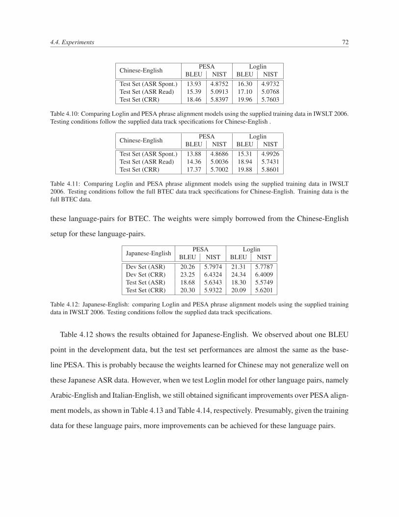
4.4. Experiments 72
Chinese-English PESA LoglinBLEU NIST BLEU NIST
Test Set (ASR Spont.) 13.93 4.8752 16.30 4.9732Test Set (ASR Read) 15.39 5.0913 17.10 5.0768Test Set (CRR) 18.46 5.8397 19.96 5.7603
Table 4.10: Comparing Loglin and PESA phrase alignment models using the supplied training data in IWSLT 2006.Testing conditions follow the supplied data track specifications for Chinese-English .
Chinese-English PESA LoglinBLEU NIST BLEU NIST
Test Set (ASR Spont.) 13.88 4.8686 15.31 4.9926Test Set (ASR Read) 14.36 5.0036 18.94 5.7431Test Set (CRR) 17.37 5.7002 19.88 5.8601
Table 4.11: Comparing Loglin and PESA phrase alignment models using the supplied training data in IWSLT2006. Testing conditions follow the full BTEC data track specifications for Chinese-English. Training data is thefull BTEC data.
these language-pairs for BTEC. The weights were simply borrowed from the Chinese-English
setup for these language-pairs.
Japanese-English PESA LoglinBLEU NIST BLEU NIST
Dev Set (ASR) 20.26 5.7974 21.31 5.7787Dev Set (CRR) 23.25 6.4324 24.34 6.4009Test Set (ASR) 18.68 5.6343 18.30 5.5749Test Set (CRR) 20.30 5.9322 20.09 5.6201
Table 4.12: Japanese-English: comparing Loglin and PESA phrase alignment models using the supplied trainingdata in IWSLT 2006. Testing conditions follow the supplied data track specifications.
Table 4.12 shows the results obtained for Japanese-English. We observed about one BLEU
point in the development data, but the test set performances are almost the same as the base-
line PESA. This is probably because the weights learned for Chinese may not generalize well on
these Japanese ASR data. However, when we test Loglin model for other language pairs, namely
Arabic-English and Italian-English, we still obtained significant improvements over PESA align-
ment models, as shown in Table 4.13 and Table 4.14, respectively. Presumably, given the training
data for these language pairs, more improvements can be achieved for these language pairs.
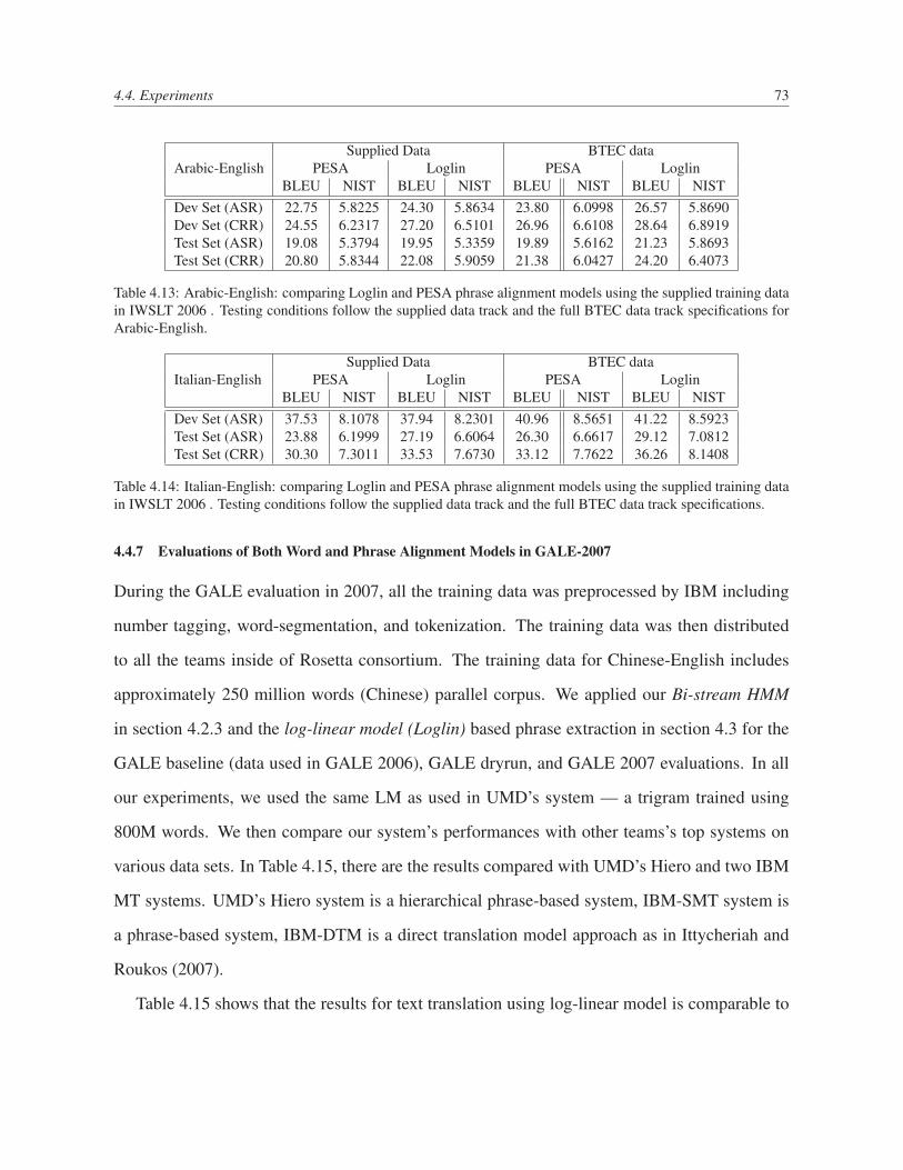
4.4. Experiments 73
Arabic-EnglishSupplied Data BTEC data
PESA Loglin PESA LoglinBLEU NIST BLEU NIST BLEU NIST BLEU NIST
Dev Set (ASR) 22.75 5.8225 24.30 5.8634 23.80 6.0998 26.57 5.8690Dev Set (CRR) 24.55 6.2317 27.20 6.5101 26.96 6.6108 28.64 6.8919Test Set (ASR) 19.08 5.3794 19.95 5.3359 19.89 5.6162 21.23 5.8693Test Set (CRR) 20.80 5.8344 22.08 5.9059 21.38 6.0427 24.20 6.4073
Table 4.13: Arabic-English: comparing Loglin and PESA phrase alignment models using the supplied training datain IWSLT 2006 . Testing conditions follow the supplied data track and the full BTEC data track specifications forArabic-English.
Italian-EnglishSupplied Data BTEC data
PESA Loglin PESA LoglinBLEU NIST BLEU NIST BLEU NIST BLEU NIST
Dev Set (ASR) 37.53 8.1078 37.94 8.2301 40.96 8.5651 41.22 8.5923Test Set (ASR) 23.88 6.1999 27.19 6.6064 26.30 6.6617 29.12 7.0812Test Set (CRR) 30.30 7.3011 33.53 7.6730 33.12 7.7622 36.26 8.1408
Table 4.14: Italian-English: comparing Loglin and PESA phrase alignment models using the supplied training datain IWSLT 2006 . Testing conditions follow the supplied data track and the full BTEC data track specifications.
4.4.7 Evaluations of Both Word and Phrase Alignment Models in GALE-2007
During the GALE evaluation in 2007, all the training data was preprocessed by IBM including
number tagging, word-segmentation, and tokenization. The training data was then distributed
to all the teams inside of Rosetta consortium. The training data for Chinese-English includes
approximately 250 million words (Chinese) parallel corpus. We applied our Bi-stream HMM
in section 4.2.3 and the log-linear model (Loglin) based phrase extraction in section 4.3 for the
GALE baseline (data used in GALE 2006), GALE dryrun, and GALE 2007 evaluations. In all
our experiments, we used the same LM as used in UMD’s system — a trigram trained using
800M words. We then compare our system’s performances with other teams’s top systems on
various data sets. In Table 4.15, there are the results compared with UMD’s Hiero and two IBM
MT systems. UMD’s Hiero system is a hierarchical phrase-based system, IBM-SMT system is
a phrase-based system, IBM-DTM is a direct translation model approach as in Ittycheriah and
Roukos (2007).
Table 4.15 shows that the results for text translation using log-linear model is comparable to

4.4. Experiments 74
System MT04 TestSetBLEU TER METEOR BLEU TER METEOR
IBM-SMT 0.3256 59.28 0.6397 0.1216 72.57 0.4610IBM-DTM 0.3022 61.54 0.6140 0.1133 72.08 0.4569UMD-Hiero 0.3123 58.13 0.6000 0.1052 72.43 0.4277CMU LogLin 0.3131 62.32 0.6308 0.1114 73.43 0.4534
Table 4.15: Translation results on Gale Dryrun for Text data in May 2007; comparing with other systems
the results from IBM and UMD. For BLEU scores, the CMU log-linear system is slightly higher
than the UMD system, and for METEOR, CMU log-linear system is better than UMD’s Hiero
system. For ASR translation, we have the results shown in Table 4.16 and Table 4.17. Overall,
the CMU log-linear system performs slightly better than UMD’s system, and close to IBM-DTM
system’s performance.
SystemBN Eval06 Dev06
BLEU TER METEOR BLEU TER METEOR BLEU TER METEOR
IBM-SMT 0.1250 79.27 0.4972 0.0748 82.22 0.3825 0.1225 81.65 0.4677IBM-DTM 0.1216 78.66 0.4955 0.0686 82.25 0.3809 0.1099 82.30 0.4596UMD-Hiero 0.1270 75.40 0.4832 0.0577 83.15 0.3542 0.1070 80.82 0.4344CMU-Loglin 0.1364 78.90 0.4987 0.0673 84.39 0.3774 0.1113 84.06 0.4565
Table 4.16: Translation results on Gale Dryrun ASR data in May-June 2007; CMU-Loglin sys comparing withother systems Part (I): using testsets of Broadcast News (BN), Gale-2006 Eval (Eval06), and Gale devset in 2006(Dev06).
SystemDev07 Shadow All
BLEU TER METEOR BLEU TER METEOR BLEU TER METEOR
IBM-SMT 0.0827 81.71 0.3895 0.0421 85.98 0.2786 0.0934 81.79 0.4136IBM-DTM 0.0742 82.25 0.3882 0.0186 90.55 0.2382 0.0841 82.27 0.4101UMD-Hiero 0.0713 82.51 0.3738 0.0237 90.98 0.2399 0.0796 82.13 0.3898CMU-Loglin 0.0806 83.59 0.3989 0.0399 91.24 0.2705 0.0875 83.89 0.4135
Table 4.17: Translation results on Gale Dryrun ASR data in May-June 2007; CMU-Loglin sys comparing withother systems Part (II): using Gale devset in 2007 (Dev07), shadow data for Gale eval in 2007 (Shadow), and all theabove datasets (All).
Score NG WL NW BN-ASR BC-ASR BN-human BC-humanBLEU 10.81 7.72 30.56 10.87 13.83 20.35 12.44NIST 4.50 3.59 8.9989 4.3020 4.2332 4.2404 4.9202
Table 4.18: Translation results on Gale Dryrun data in April 2006. NG: news group, WL: web-log, NW: news wire,BN-ASR: Broadcast news ASR output, BC-ASR: Broadcast conversation ASR output, BN-human: Broadcast newshuman transcript, BC-human: Broadcast conversation human transcription.
4.5. Discussions and Summary 75
We also did system combination experiments 1 for two CMU internal MT systems: the blocks
for SMT Loglin system are based on the log-linear model, and they were further re-scored for
each document using the techniques described in Chapt. 6; the syntax-augmented system was
done by Venugopal et al. (2007). As the CMU-Syntax only submitted the text translations,
we here compare the systems performances using the shadow data for text for the GALE-2007
evaluation.
Shown in Table 4.19 are the submitted results from each group. CMU-Loglin-reanked is
a simple re-ranking for 1K-best list from CMU-Loglin system using IBM Model-1 features.
Overall, CMU-Loglin has significantly better BLEU than CMU-syntax esp. on top-shadow
data. CMU-syntax system seems to generate shorter translations, and therefore, it has better
precision and TER. The system combination acts as balance for selecting translations from both
the CMU-Loglin and CMU-Syntax systems, and the final score metrics we got are very close
to the top scores under each data settings. This experiment reveals one more utility for using
the proposed Loglin SMT for system combinations. The final Rosetta submission for GALE07
was based on several configurations of combinations using these individual systems and their
reranked versions; more details are in Huang and Papineni (2007).
4.5 Discussions and Summary
The professional translators using multiple information sources in translating is a fact that is
not yet addressed well in current machine translation models. The information streams beyond
word-surface level can enhance the expressive power of translation models especially for low-
density language-pairs as exemplified in the small-data track for Chinese-English.
In this chapter, modeling with multiple information streams for word-alignment and for
phrase-extraction are proposed and tested on both small and large data sets. The proposed mod-
els share the characteristics of handling overlapped features and the flexibility of incorporating
new information streams. In our experiments, we showed the utilities of bilingual word-clusters1ack: help from Silja
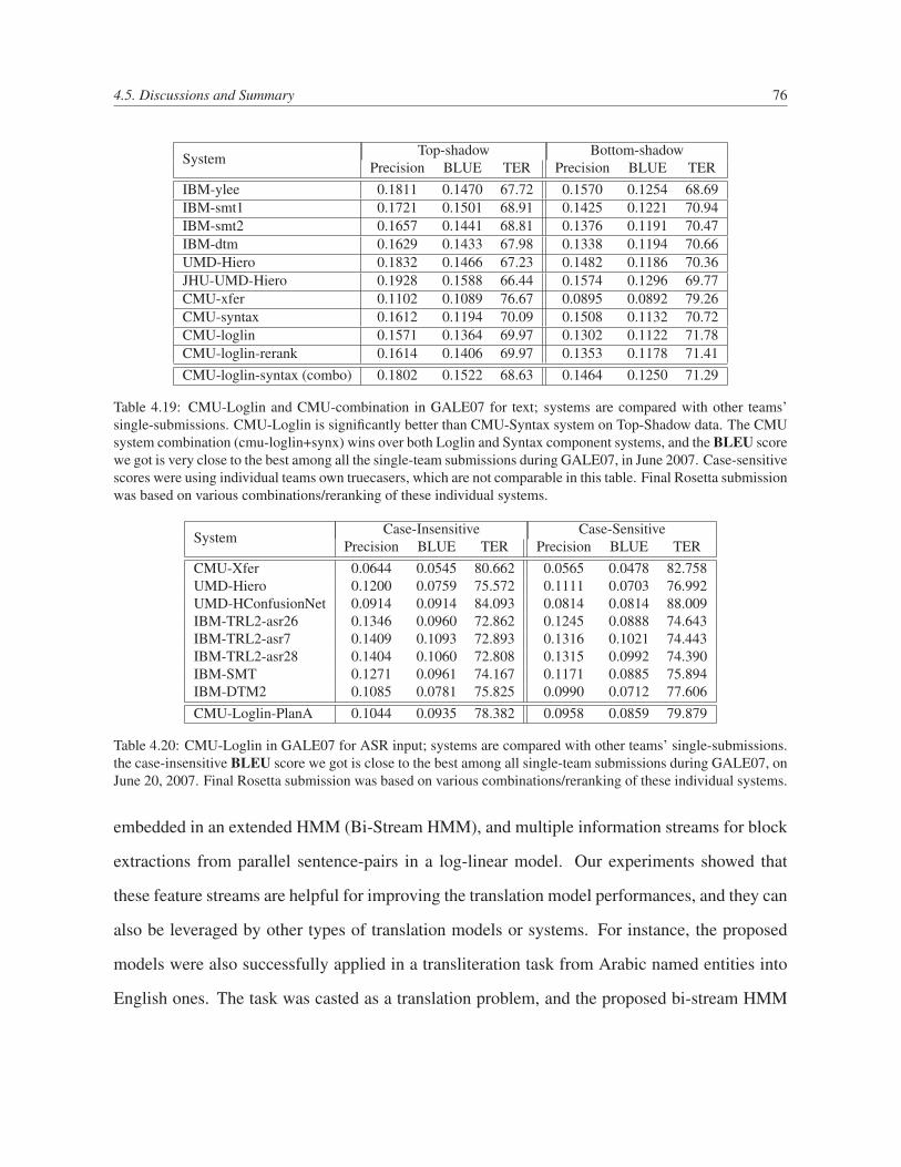
4.5. Discussions and Summary 76
System Top-shadow Bottom-shadowPrecision BLUE TER Precision BLUE TER
IBM-ylee 0.1811 0.1470 67.72 0.1570 0.1254 68.69IBM-smt1 0.1721 0.1501 68.91 0.1425 0.1221 70.94IBM-smt2 0.1657 0.1441 68.81 0.1376 0.1191 70.47IBM-dtm 0.1629 0.1433 67.98 0.1338 0.1194 70.66UMD-Hiero 0.1832 0.1466 67.23 0.1482 0.1186 70.36JHU-UMD-Hiero 0.1928 0.1588 66.44 0.1574 0.1296 69.77CMU-xfer 0.1102 0.1089 76.67 0.0895 0.0892 79.26CMU-syntax 0.1612 0.1194 70.09 0.1508 0.1132 70.72CMU-loglin 0.1571 0.1364 69.97 0.1302 0.1122 71.78CMU-loglin-rerank 0.1614 0.1406 69.97 0.1353 0.1178 71.41CMU-loglin-syntax (combo) 0.1802 0.1522 68.63 0.1464 0.1250 71.29
Table 4.19: CMU-Loglin and CMU-combination in GALE07 for text; systems are compared with other teams’single-submissions. CMU-Loglin is significantly better than CMU-Syntax system on Top-Shadow data. The CMUsystem combination (cmu-loglin+synx) wins over both Loglin and Syntax component systems, and the BLEU scorewe got is very close to the best among all the single-team submissions during GALE07, in June 2007. Case-sensitivescores were using individual teams own truecasers, which are not comparable in this table. Final Rosetta submissionwas based on various combinations/reranking of these individual systems.
System Case-Insensitive Case-SensitivePrecision BLUE TER Precision BLUE TER
CMU-Xfer 0.0644 0.0545 80.662 0.0565 0.0478 82.758UMD-Hiero 0.1200 0.0759 75.572 0.1111 0.0703 76.992UMD-HConfusionNet 0.0914 0.0914 84.093 0.0814 0.0814 88.009IBM-TRL2-asr26 0.1346 0.0960 72.862 0.1245 0.0888 74.643IBM-TRL2-asr7 0.1409 0.1093 72.893 0.1316 0.1021 74.443IBM-TRL2-asr28 0.1404 0.1060 72.808 0.1315 0.0992 74.390IBM-SMT 0.1271 0.0961 74.167 0.1171 0.0885 75.894IBM-DTM2 0.1085 0.0781 75.825 0.0990 0.0712 77.606CMU-Loglin-PlanA 0.1044 0.0935 78.382 0.0958 0.0859 79.879
Table 4.20: CMU-Loglin in GALE07 for ASR input; systems are compared with other teams’ single-submissions.the case-insensitive BLEU score we got is close to the best among all single-team submissions during GALE07, onJune 20, 2007. Final Rosetta submission was based on various combinations/reranking of these individual systems.
embedded in an extended HMM (Bi-Stream HMM), and multiple information streams for block
extractions from parallel sentence-pairs in a log-linear model. Our experiments showed that
these feature streams are helpful for improving the translation model performances, and they can
also be leveraged by other types of translation models or systems. For instance, the proposed
models were also successfully applied in a transliteration task from Arabic named entities into
English ones. The task was casted as a translation problem, and the proposed bi-stream HMM
4.5. Discussions and Summary 77
and log-linear phrase-alignment models were configured for letter-sequence within a named-
entity. Significant improved results were obtained over IBM models as shown in Zhao et al.
(2007).
The proposed models provided clues to improve baseline word and phrase-alignment models.
The features regarding the inside and outside of the block given the sentence-pair context can
be combined in the learning loop of a generative model. In this way, the model parameters
will benefit from not only the local decisions as in the traditional EM, but also the fractional
counts collected from the decisions which take into considerations from the context outside of
the blocks. The model of “Inner-Outer Bracket Model” in Chapt. 5 is one such example.
Chapter 5
Modeling Hidden Blocks
Modeling translation equivalence on the phrase-pair level gives state-of-the-art machine trans-
lation performances. The potential reasons are better modeling of contexts and local word re-
ordering. It is also less sensitive to the errors in the preprocessing steps.
In Chapt. 4, several feature functions were proposed using the context inside of a block and
outside of a block. These features were shown to be helpful for improving the phrase-alignment.
However, the log-linear model does not feed these features streams into the iterative learning
loop for updating the model parameters and improve the accuracies of the blocks. In this chapter,
each block induces a segmentation of the sentence-pair, and introduces a soft decision for the
word alignment inside and outside of the block. This process is introduced in the EM learning
loop for updating the word alignment and block segmentation iteratively.
We propose a new method for localizing word alignments as in (Zhao et al., 2005). We use
blocks to achieve locality decisions in the following manner: the inner part of the block in a
sentence pair is a source phrase aligned to a target phrase. We assume that words inside the
source phrase cannot align to words outside the target phrase and that words outside the source
phrase cannot align to words inside the target phrase. Furthermore, a block divides the sentence
pair into two smaller regions: the inner part of the block, which corresponds to the source and
78
5.1. Segmentation of Blocks 79
target phrase in the block, and the outer part of the block, which corresponds to the remaining
source and target words in the parallel sentence pair. The two regions are non-overlapping; and
each of them is shorter in length than the original parallel sentence pair. The regions are thus
easier to align than the original sentence pairs (e.g., using IBM Model-1), assuming the given
block is a perfect one. While the model uses a single block to split the sentence pair into two
independent regions, it is not clear which block we should select for this purpose. Therefore, we
treat the splitting block as a hidden variable.
5.1 Segmentation of Blocks
We use the following notation in the remainder of this chapter: e and f denote the English
and foreign sentences with sentence lengths of I and J , respectively. ei is an English word at
position i in e; fj is a foreign word at position j in f . a is the alignment vector with aj mapping
the position of the English word eajto which fj connects. We have the common limitation in
this representation that one foreign word cannot be connected to more than one English word. A
block δ[] is defined as a pair of brackets as follows:
δ[] = (δe, δf ) = ([il, ir], [jl, jr]), (5.1)
where δe = [il, ir] is a bracket in the English sentence defined by a pair of indices: the left
position il and the right position ir, corresponding to a English phrase eiril
. Similar notations
are for δf = [jl, jr], which is one possible projection of δe in f . The subscript l and r are
abbreviations of left and right, respectively.
δe segments e into two parts: (δe, e) = (δe∈, δ
e/∈). The inner part δe
∈ = {ei, i ∈ [il, ir]} and the
outer part δe/∈ = {ei, i /∈ [il, ir]}; δf segments f similarly.
Thus, the block δ[] splits the parallel sentence pair into two non-overlapping regions: the
Inner δ[]∈ and Outer δ
[]/∈ parts (see Figure 5.1). With this segmentation, we assume the words in
the inner part are aligned to words in the inner part only: δ[]∈ = δe
∈ ↔ δf∈ : {ei, i ∈ [il, ir]} ↔

5.2. Inner-Outer Bracketing Models with Hidden Blocks 80
Outer
Inner
li ri
rj
lj
eδ
fδ
Figure 5.1: Parallel Sentence-Pair Segmentation by a Block
{fj, j ∈ [jl, jr]}; and words in the outer part are aligned to words in the outer part only: δ[]/∈ =
δe/∈ ↔ δf
/∈ : {ei, i /∈ [il, ir]} ↔ {fj, j /∈ [jl, jr]}. We do not allow alignments to cross block
boundaries. Words inside a block δ[] can be aligned using a variety of models (IBM models 1-5,
HMM, etc). We choose Model1 for simplicity. In the learning loop, if the block boundaries are
accurate, we can expect high quality word alignment, and vice versa. This is our proposed new
localization method.
5.2 Inner-Outer Bracketing Models with Hidden Blocks
We treat the constraining block as a hidden variable in a generative model shown in Eqn. 5.2.
P (f |e) =∑
{δ[]}P (f , δ[]|e)
=∑
{δe}
∑
{δf}P (f , δf |δe, e)P (δe|e), (5.2)
where δ[] = (δe, δf ) is the hidden block. In the generative process, the model first generates a
bracket δe for e with a monolingual bracketing model of P (δe|e). It then uses the segmentation
of the English (δe, e) to generate the projected bracket δf of f using a generative translation
model P (f , δf |δe, e) = P (δf/∈, δ
f∈|δe
/∈, δe∈) — the key model to implement our proposed inner-
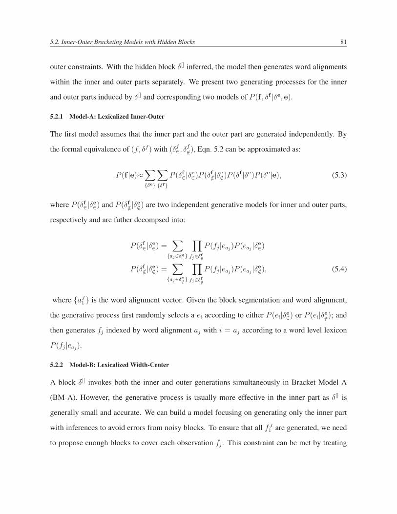
5.2. Inner-Outer Bracketing Models with Hidden Blocks 81
outer constraints. With the hidden block δ[] inferred, the model then generates word alignments
within the inner and outer parts separately. We present two generating processes for the inner
and outer parts induced by δ[] and corresponding two models of P (f , δf |δe, e).
5.2.1 Model-A: Lexicalized Inner-Outer
The first model assumes that the inner part and the outer part are generated independently. By
the formal equivalence of (f, δf ) with (δf∈, δ
f/∈), Eqn. 5.2 can be approximated as:
P (f |e)≈∑
{δe}
∑
{δf}P (δf
∈|δe∈)P (δf
/∈|δe/∈)P (δf |δe)P (δe|e), (5.3)
where P (δf∈|δe
∈) and P (δf/∈|δe
/∈) are two independent generative models for inner and outer parts,
respectively and are futher decompsed into:
P (δf∈|δe
∈) =∑
{aj∈δe∈}
∏
fj∈δf∈
P (fj|eaj)P (eaj
|δe∈)
P (δf/∈|δe
/∈) =∑
{aj∈δe/∈}
∏
fj∈δf/∈
P (fj|eaj)P (eaj
|δe/∈), (5.4)
where {aJ1} is the word alignment vector. Given the block segmentation and word alignment,
the generative process first randomly selects a ei according to either P (ei|δe∈) or P (ei|δe
/∈); and
then generates fj indexed by word alignment aj with i = aj according to a word level lexicon
P (fj|eaj).
5.2.2 Model-B: Lexicalized Width-Center
A block δ[] invokes both the inner and outer generations simultaneously in Bracket Model A
(BM-A). However, the generative process is usually more effective in the inner part as δ[] is
generally small and accurate. We can build a model focusing on generating only the inner part
with inferences to avoid errors from noisy blocks. To ensure that all fJ1 are generated, we need
to propose enough blocks to cover each observation fj . This constraint can be met by treating
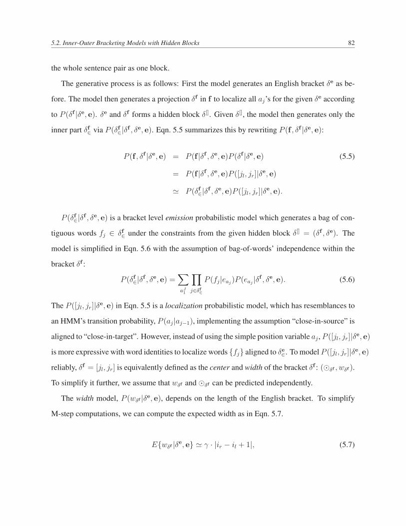
5.2. Inner-Outer Bracketing Models with Hidden Blocks 82
the whole sentence pair as one block.
The generative process is as follows: First the model generates an English bracket δe as be-
fore. The model then generates a projection δf in f to localize all aj’s for the given δe according
to P (δf |δe, e). δe and δf forms a hidden block δ[]. Given δ[], the model then generates only the
inner part δf∈ via P (δf
∈|δf , δe, e). Eqn. 5.5 summarizes this by rewriting P (f , δf |δe, e):
P (f , δf |δe, e) = P (f |δf , δe, e)P (δf |δe, e) (5.5)
= P (f |δf , δe, e)P ([jl, jr]|δe, e)
' P (δf∈|δf , δe, e)P ([jl, jr]|δe, e).
P (δf∈|δf , δe, e) is a bracket level emission probabilistic model which generates a bag of con-
tiguous words fj ∈ δf∈ under the constraints from the given hidden block δ[] = (δf , δe). The
model is simplified in Eqn. 5.6 with the assumption of bag-of-words’ independence within the
bracket δf :
P (δf∈|δf , δe, e) =
∑
aJ1
∏
j∈δf∈
P (fj|eaj)P (eaj
|δf , δe, e). (5.6)
The P ([jl, jr]|δe, e) in Eqn. 5.5 is a localization probabilistic model, which has resemblances to
an HMM’s transition probability, P (aj|aj−1), implementing the assumption “close-in-source” is
aligned to “close-in-target”. However, instead of using the simple position variable aj , P ([jl, jr]|δe, e)
is more expressive with word identities to localize words {fj} aligned to δe∈. To model P ([jl, jr]|δe, e)
reliably, δf = [jl, jr] is equivalently defined as the center and width of the bracket δf : (¯δf , wδf ).
To simplify it further, we assume that wδf and ¯δf can be predicted independently.
The width model, P (wδf |δe, e), depends on the length of the English bracket. To simplify
M-step computations, we can compute the expected width as in Eqn. 5.7.
E{wδf |δe, e} ' γ · |ir − il + 1|, (5.7)
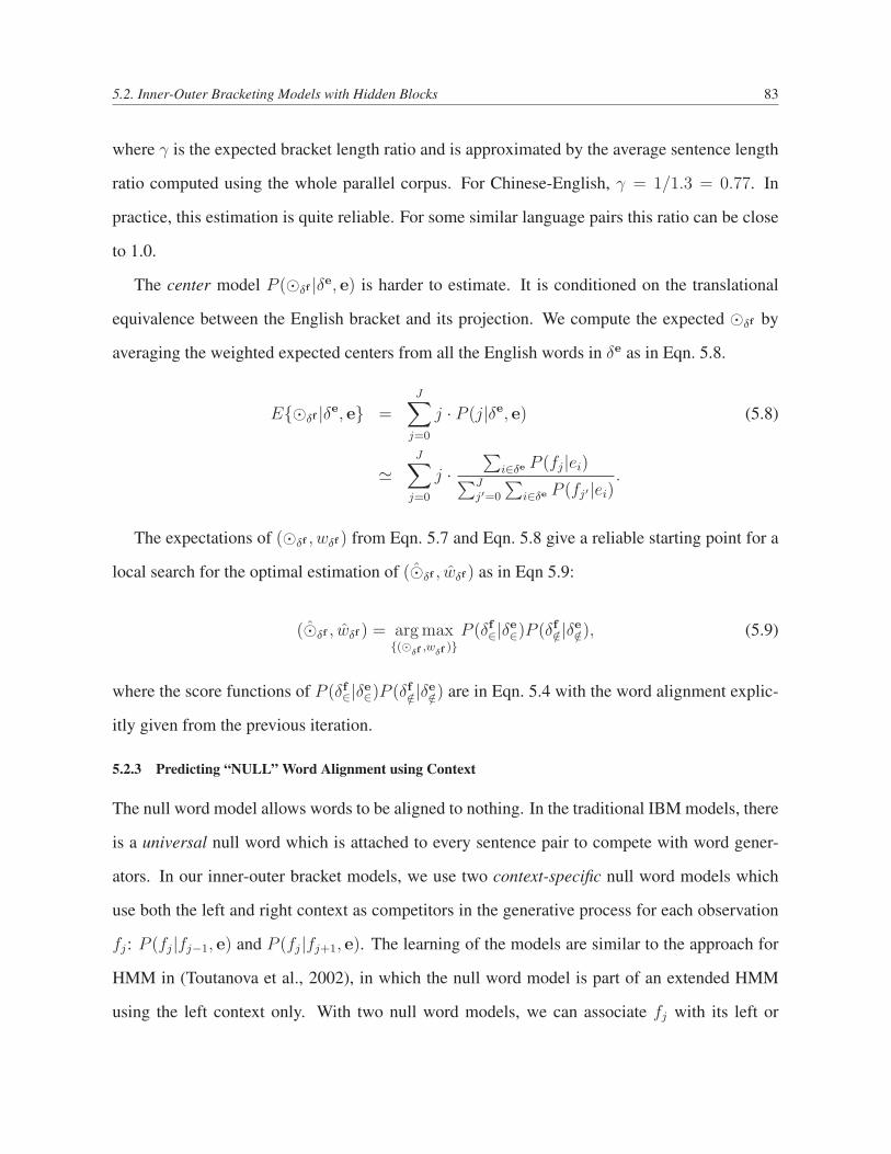
5.2. Inner-Outer Bracketing Models with Hidden Blocks 83
where γ is the expected bracket length ratio and is approximated by the average sentence length
ratio computed using the whole parallel corpus. For Chinese-English, γ = 1/1.3 = 0.77. In
practice, this estimation is quite reliable. For some similar language pairs this ratio can be close
to 1.0.
The center model P (¯δf |δe, e) is harder to estimate. It is conditioned on the translational
equivalence between the English bracket and its projection. We compute the expected ¯δf by
averaging the weighted expected centers from all the English words in δe as in Eqn. 5.8.
E{¯δf |δe, e} =J∑
j=0
j · P (j|δe, e) (5.8)
'J∑
j=0
j ·∑
i∈δe P (fj|ei)∑Jj′=0
∑i∈δe P (fj′|ei)
.
The expectations of (¯δf , wδf ) from Eqn. 5.7 and Eqn. 5.8 give a reliable starting point for a
local search for the optimal estimation of ( ˆδf , wδf ) as in Eqn 5.9:
( ˆδf , wδf ) = arg max
{(¯δf
,wδf
)}P (δf
∈|δe∈)P (δf
/∈|δe/∈), (5.9)
where the score functions of P (δf∈|δe
∈)P (δf/∈|δe
/∈) are in Eqn. 5.4 with the word alignment explic-
itly given from the previous iteration.
5.2.3 Predicting “NULL” Word Alignment using Context
The null word model allows words to be aligned to nothing. In the traditional IBM models, there
is a universal null word which is attached to every sentence pair to compete with word gener-
ators. In our inner-outer bracket models, we use two context-specific null word models which
use both the left and right context as competitors in the generative process for each observation
fj: P (fj|fj−1, e) and P (fj|fj+1, e). The learning of the models are similar to the approach for
HMM in (Toutanova et al., 2002), in which the null word model is part of an extended HMM
using the left context only. With two null word models, we can associate fj with its left or
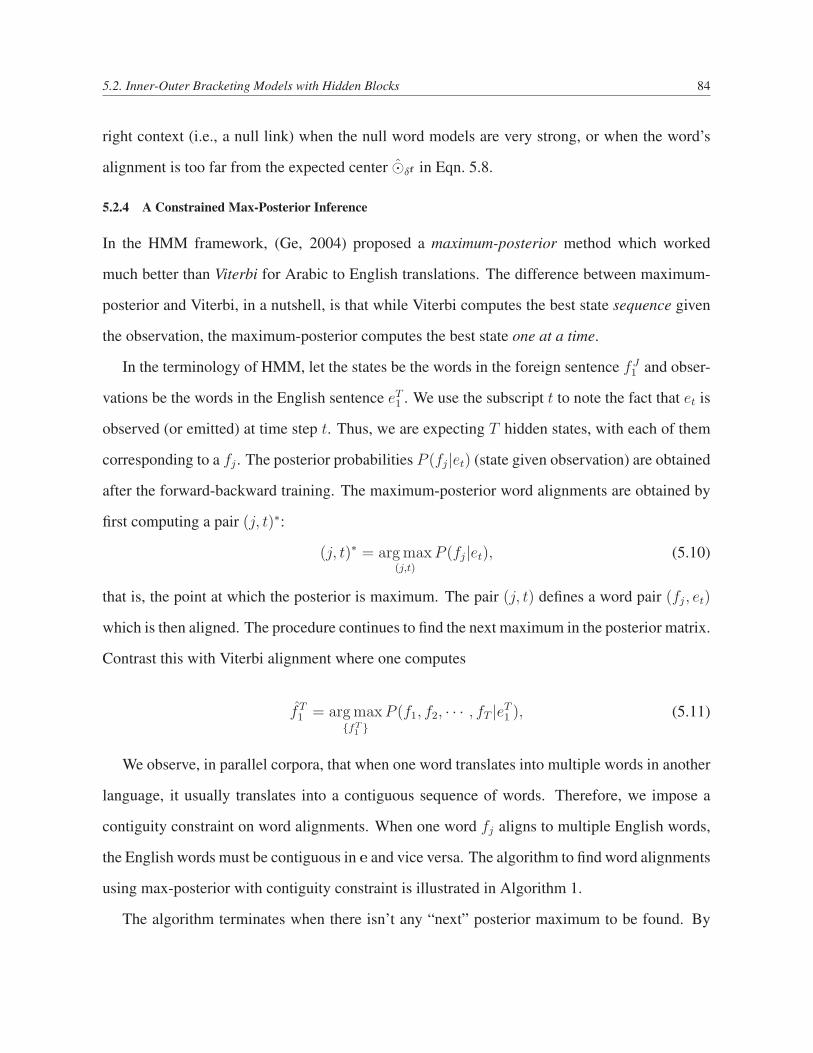
5.2. Inner-Outer Bracketing Models with Hidden Blocks 84
right context (i.e., a null link) when the null word models are very strong, or when the word’s
alignment is too far from the expected center ˆδf in Eqn. 5.8.
5.2.4 A Constrained Max-Posterior Inference
In the HMM framework, (Ge, 2004) proposed a maximum-posterior method which worked
much better than Viterbi for Arabic to English translations. The difference between maximum-
posterior and Viterbi, in a nutshell, is that while Viterbi computes the best state sequence given
the observation, the maximum-posterior computes the best state one at a time.
In the terminology of HMM, let the states be the words in the foreign sentence fJ1 and obser-
vations be the words in the English sentence eT1 . We use the subscript t to note the fact that et is
observed (or emitted) at time step t. Thus, we are expecting T hidden states, with each of them
corresponding to a fj . The posterior probabilities P (fj|et) (state given observation) are obtained
after the forward-backward training. The maximum-posterior word alignments are obtained by
first computing a pair (j, t)∗:
(j, t)∗ = arg max(j,t)
P (fj|et), (5.10)
that is, the point at which the posterior is maximum. The pair (j, t) defines a word pair (fj, et)
which is then aligned. The procedure continues to find the next maximum in the posterior matrix.
Contrast this with Viterbi alignment where one computes
fT1 = arg max
{fT1 }
P (f1, f2, · · · , fT |eT1 ), (5.11)
We observe, in parallel corpora, that when one word translates into multiple words in another
language, it usually translates into a contiguous sequence of words. Therefore, we impose a
contiguity constraint on word alignments. When one word fj aligns to multiple English words,
the English words must be contiguous in e and vice versa. The algorithm to find word alignments
using max-posterior with contiguity constraint is illustrated in Algorithm 1.
The algorithm terminates when there isn’t any “next” posterior maximum to be found. By
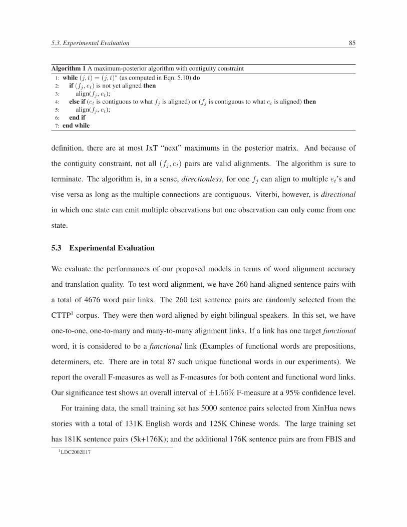
5.3. Experimental Evaluation 85
Algorithm 1 A maximum-posterior algorithm with contiguity constraint1: while (j, t) = (j, t)∗ (as computed in Eqn. 5.10) do2: if (fj , et) is not yet aligned then3: align(fj , et);4: else if (et is contiguous to what fj is aligned) or (fj is contiguous to what et is aligned) then5: align(fj , et);6: end if7: end while
definition, there are at most JxT “next” maximums in the posterior matrix. And because of
the contiguity constraint, not all (fj, et) pairs are valid alignments. The algorithm is sure to
terminate. The algorithm is, in a sense, directionless, for one fj can align to multiple et’s and
vise versa as long as the multiple connections are contiguous. Viterbi, however, is directional
in which one state can emit multiple observations but one observation can only come from one
state.
5.3 Experimental Evaluation
We evaluate the performances of our proposed models in terms of word alignment accuracy
and translation quality. To test word alignment, we have 260 hand-aligned sentence pairs with
a total of 4676 word pair links. The 260 test sentence pairs are randomly selected from the
CTTP1 corpus. They were then word aligned by eight bilingual speakers. In this set, we have
one-to-one, one-to-many and many-to-many alignment links. If a link has one target functional
word, it is considered to be a functional link (Examples of functional words are prepositions,
determiners, etc. There are in total 87 such unique functional words in our experiments). We
report the overall F-measures as well as F-measures for both content and functional word links.
Our significance test shows an overall interval of ±1.56% F-measure at a 95% confidence level.
For training data, the small training set has 5000 sentence pairs selected from XinHua news
stories with a total of 131K English words and 125K Chinese words. The large training set
has 181K sentence pairs (5k+176K); and the additional 176K sentence pairs are from FBIS and1LDC2002E17
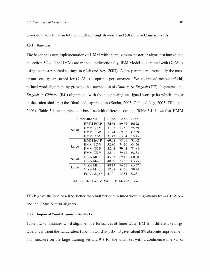
5.3. Experimental Evaluation 86
Sinorama, which has in total 6.7 million English words and 5.8 million Chinese words.
5.3.1 Baselines
The baseline is our implementation of HMM with the maximum-posterior algorithm introduced
in section 5.2.4. The HMMs are trained unidirectionally. IBM Model-4 is trained with GIZA++
using the best reported settings in (Och and Ney, 2003). A few parameters, especially the max-
imum fertility, are tuned for GIZA++’s optimal performance. We collect bi-directional (bi)
refined word alignment by growing the intersection of Chinese-to-English (CE) alignments and
English-to-Chinese (EC) alignments with the neighboring unaligned word pairs which appear
in the union similar to the “final-and” approaches (Koehn, 2003; Och and Ney, 2003; Tillmann,
2003). Table 5.1 summarizes our baseline with different settings. Table 5.1 shows that HMM
F-measure(%) Func Cont Both
Small
HMM EC-P 54.69 69.99 64.78HMM EC-V 31.38 53.56 55.59HMM CE-P 51.44 69.35 62.69HMM CE-V 31.43 63.84 55.45
Large
HMM EC-P 60.08 78.01 71.92HMM EC-V 32.80 74.10 64.26HMM CE-P 58.45 79.44 71.84HMM CE-V 35.41 79.12 68.33
Small GIZA MH-bi 45.63 69.48 60.08GIZA M4-bi 48.80 73.68 63.75
Large GIZA MH-bi 49.13 76.51 65.67GIZA M4-bi 52.88 81.76 70.24
- Fully-Align 2 5.10 15.84 9.28
Table 5.1: Baseline: V: Viterbi; P: Max-Posterior
EC-P gives the best baseline, better than bidirectional refined word alignments from GIZA M4
and the HMM Viterbi aligners.
5.3.2 Improved Word Alignment via Blocks
Table 5.2 summarizes word alignment performances of Inner-Outer BM-B in different settings.
Overall, without the handcrafted function word list, BM-B gives about 8% absolute improvement
in F-measure on the large training set and 9% for the small set with a confidence interval of
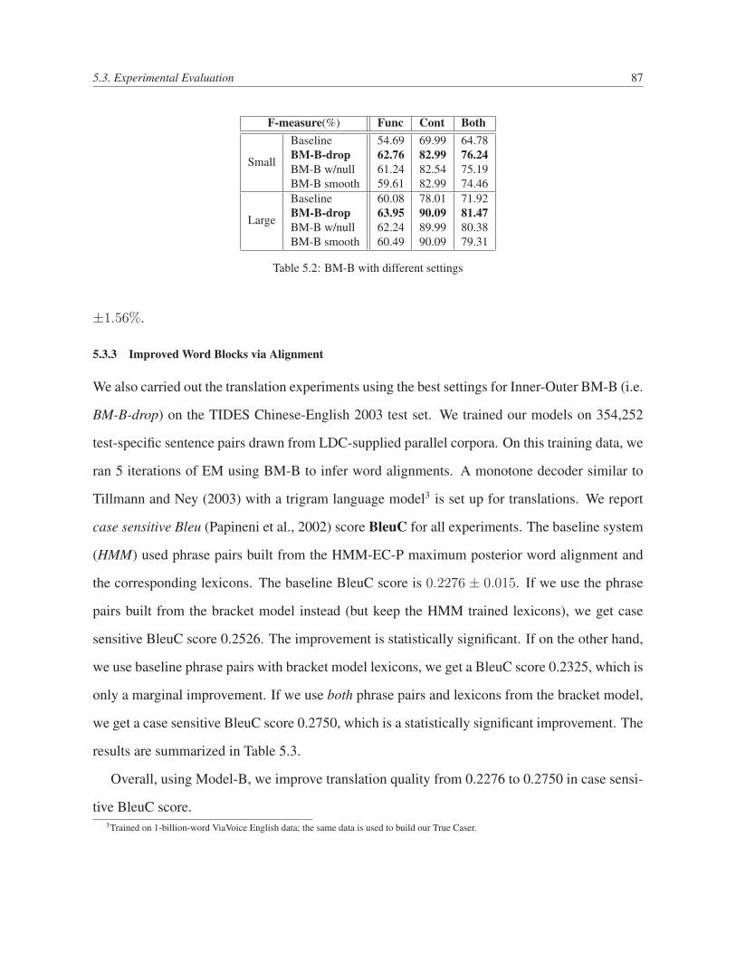
5.3. Experimental Evaluation 87
F-measure(%) Func Cont Both
Small
Baseline 54.69 69.99 64.78BM-B-drop 62.76 82.99 76.24BM-B w/null 61.24 82.54 75.19BM-B smooth 59.61 82.99 74.46
Large
Baseline 60.08 78.01 71.92BM-B-drop 63.95 90.09 81.47BM-B w/null 62.24 89.99 80.38BM-B smooth 60.49 90.09 79.31
Table 5.2: BM-B with different settings
±1.56%.
5.3.3 Improved Word Blocks via Alignment
We also carried out the translation experiments using the best settings for Inner-Outer BM-B (i.e.
BM-B-drop) on the TIDES Chinese-English 2003 test set. We trained our models on 354,252
test-specific sentence pairs drawn from LDC-supplied parallel corpora. On this training data, we
ran 5 iterations of EM using BM-B to infer word alignments. A monotone decoder similar to
Tillmann and Ney (2003) with a trigram language model3 is set up for translations. We report
case sensitive Bleu (Papineni et al., 2002) score BleuC for all experiments. The baseline system
(HMM) used phrase pairs built from the HMM-EC-P maximum posterior word alignment and
the corresponding lexicons. The baseline BleuC score is 0.2276 ± 0.015. If we use the phrase
pairs built from the bracket model instead (but keep the HMM trained lexicons), we get case
sensitive BleuC score 0.2526. The improvement is statistically significant. If on the other hand,
we use baseline phrase pairs with bracket model lexicons, we get a BleuC score 0.2325, which is
only a marginal improvement. If we use both phrase pairs and lexicons from the bracket model,
we get a case sensitive BleuC score 0.2750, which is a statistically significant improvement. The
results are summarized in Table 5.3.
Overall, using Model-B, we improve translation quality from 0.2276 to 0.2750 in case sensi-
tive BleuC score.3Trained on 1-billion-word ViaVoice English data; the same data is used to build our True Caser.
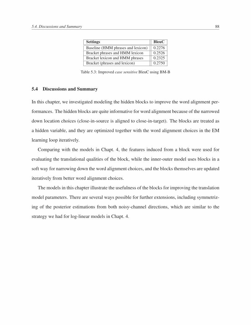
5.4. Discussions and Summary 88
Settings BleuCBaseline (HMM phrases and lexicon) 0.2276Bracket phrases and HMM lexicon 0.2526Bracket lexicon and HMM phrases 0.2325Bracket (phrases and lexicon) 0.2750
Table 5.3: Improved case sensitive BleuC using BM-B
5.4 Discussions and Summary
In this chapter, we investigated modeling the hidden blocks to improve the word alignment per-
formances. The hidden blocks are quite informative for word alignment because of the narrowed
down location choices (close-in-source is aligned to close-in-target). The blocks are treated as
a hidden variable, and they are optimized together with the word alignment choices in the EM
learning loop iteratively.
Comparing with the models in Chapt. 4, the features induced from a block were used for
evaluating the translational qualities of the block, while the inner-outer model uses blocks in a
soft way for narrowing down the word alignment choices, and the blocks themselves are updated
iteratively from better word alignment choices.
The models in this chapter illustrate the usefulness of the blocks for improving the translation
model parameters. There are several ways possible for further extensions, including symmetriz-
ing of the posterior estimations from both noisy-channel directions, which are similar to the
strategy we had for log-linear models in Chapt. 4.
Chapter 6
Modeling Hidden Concepts in Translation
Statistical machine translation has been treating parallel data as independent sentence-pairs
whether or not they are from the same document-pair. Translation models are learned only at
sentence-pair level. The goal of machine translation — to translate documents — has generally
been overlooked therefore. In fact, translating documents differ considerably from translating
a group of unrelated sentences. One should avoid destroying a coherent document by simply
translating it into a group of sentences which are unrelated to each other and detached from the
context.
Recent developments in statistics, genetics and machine learning show that latent topical
aspects of complex data can often be captured by a model known as statistical admixture (or
mixed membership model). Statistically, an object is said to be derived from an admixture if
it consists of a bag of elements, each sampled independently or coupled in certain ways, from
a mixture model. In the context of SMT, each parallel document-pair is treated as an object.
Depending on the chosen modeling granularity, all sentence-pairs or word-pairs in a document-
pair correspond to the basic elements constituting the object, and the mixture from which the
elements are sampled can correspond to a collection of translation lexicons based on different
topics (e.g., economics, politics, sports, etc.). Variants of such admixture models have appeared
89
90
in population genetics (Pritchard et al., 2000) and text modeling (Blei et al., 2003; Erosheva
et al., 2004). Recently, we proposed a Bilingual Topic-AdMixture (BiTAM) in Zhao and Xing
(2006) to model the topical mixtures underlying SMT; this enables word-pairs, from a paral-
lel document, to be induced according to topic-specific translation lexicons. Simple BiTAMs,
which are generalizations of IBM Model-1, are very efficient to learn, and scalable for large
training data. However, they do not capture locality constraints of word alignment, i.e., words
“close-in-source” are usually aligned to words “close-in-target”, under topical contagion. To
incorporate such local constraints for BiTAMs, we conjoin the advantages of both the HMM and
the BiTAMs, and propose a Hidden Markov Bilingual Topic-AdMixture model, or HM-BiTAM
as in Zhao and Xing (2007), for word alignment that leverages on both locality constraints and
topical context from parallel document-pair.
Previous related works include those inferring non-overlapping bilingual word clusters (Wang
et al., 1996; Och, 1999; Zhao et al., 2005) with particular translation models. The non-overlapping
word-clusters were shown to be effective for enriching the alignment dependencies; they also im-
proved the alignment quality. The proposed approach, in this thesis, can be considered as soft
clustering algorithms, in which a word belongs to a vector of weighted topics rather than one
single cluster/class. There is a weight associated with each of the topic for the word. This is
in the same spirit of the Latent Dirichlet Allocation (LDA) (Blei et al., 2003) for monolingual
mixture of unigrams. We extend bilingual lexicon mixtures by leveraging a Dirichlet prior over
topic mixture weights (e.g., prior proportions). Each topic, in the proposed model, corresponds
to a point in a conditional simplex: each source word invokes a simplex, in which each dimen-
sion corresponds to a bilingual translation candidate. The hidden topics are leveraged in learning
topic-specific bilingual translation lexicons, to enrich the emission distribution of IBM models
or HMM, and thereby improve their expressiveness. Under this framework, bilingual statistics
are shared more effectively across different topics. Constrained by the hidden topics, a word will
have only limited translation candidates. The translation models, therefore, are expected to be
6.1. Notations and Terminology 91
smaller and sharper.
6.1 Notations and Terminology
Before introducing the latent variables to capture the abstract notations of bilingual topics, we
start from a revisit to the parallel data to identify the entities in the proposed BiTAM models
such as “word-pair”, “sentence-pair” and “document-pair”. We formally define the following
terms:
• A word-pair (fj, ei) is the basic unit discrete data for machine translation, where fj is a
French word and ei is an English word. j and i are the positions in the corresponding
French sentence f and English sentence e.
• A sentence-pair (f , e) contains the source sentence f with a length of J : f = f1, f2, · · · , fj, · · · , fJ ;
a target sentence e with a length of I: e = e1, e2, · · · , ei,
· · · , eI . The two sentences f and e are considered to be the translations of each other.
• A document pair (F,E) contains two documents: the source document F and the tar-
get document E, which are mutual translations of each other. F has N sentences: F =
{fn|n = 1, · · · , N}. For simplicity, let’s assume the sentence-level alignment is one-to-
one mapping. Therefore, a document-pair has a sequence of N parallel sentence-pairs
{(fn, en)|n = 1 · · ·N}, where (fn, en) is the n’th parallel sentence-pair.
• A parallel corpus C is a collection of M parallel document-pairs: {(F,E)d|d = 1, · · · ,M}.
For notations used in the noisy channel model, we denote the French monolingual corpus as
CF and English part as CE . We are using the end-user terminology: French is the source
language, and English is the target language throughout this thesis. We are translating
Foreign language (e.g., French) into English.
6.2. Admixture of Topics for Parallel Data 92
For traditional statistical machine translation (Brown et al., 1993), the noisy-channel model
is used to describe the decoding process as shown below:
e∗ = arg max{e}
P (e|f)
= arg max{e}
P (f |e)P (e), (6.1)
where e is a English sentence, decoded as the translation of the source sentence f ; P (f |e) is the
translation model, for example, the traditional IBM Model 1 ∼ 5 and HMM; P (e) is a language
model, such as a trigram.
Now, the translation model can be extended to the document-level using the notations given
above. Instead of translating at the sentence-level, we are able to translate at the document-level,
shown in Eqn. 6.2:
CE∗ = arg max
{CE}P (CE|CF )
= arg max{CE}
P (CF |CE)P (CE), (6.2)
where P (CF |CE) is a document-level translation model: a generative model for the whole
document of CF as one entity. In this model, we are able to introduce the topics for each
document-pair to improve the model’s expressive power. Rather than being translated into un-
related segments and then pieced them together later on, as presented in traditional approaches,
the sentences in the new model can be meaningfully connected and integrated during translation
by the topics in the documents. Since the document is treated as a whole entity, the translation
is more coherent consequently.
6.2 Admixture of Topics for Parallel Data
A document-pair (F,E) is treated as an admixture of topics, which is induced by random draws
of a topic, from a pool of topics; the sentence-pairs are then generated according to the topic-
6.2. Admixture of Topics for Parallel Data 93
assignment. A unique normalized and real-valued vector θ, referred to as a topic-weight vector,
captures the contribution of different topics and is instantiated for each document-pair, so that
the sentence-pairs with their alignments are generated from topics mixed according to these
common proportions. Marginally, a sentence-pair is word-aligned according to a unique topic-
specific bilingual model given the hidden topical assignments. Therefore, the sentence-level
translations are coupled, rather than being independent as assumed in the IBM models or HMM
and their extensions.
I will introduce the proposed models for this document-level translation model, by starting
from extending IBM Model-1 to BiTAM Model-1, and then from HMM, with similar deriva-
tions, to the final model of HM-BiTAM.
6.2.1 Bilingual AdMixture Model: BiTAM Model-1
The first model BiTAM Model-1, a generative model of a parallel document proposed within
this BiTAM framework, generalizes over the simplest IBM models, e.g., IBM Model-1 word
alignment. The key idea is that each parallel document is represented as random mixtures over
a set of latent topics, in which each topic is characterized by a distribution over word-pairs.
6.2.2 The Sampling Scheme for BiTAM Model-1
The generative process (i.e., sampling process) for a parallel document-pair (F,E) is described
as below:
1. Sample number of sentence-pairs N from a Poisson(γ).
2. Sample topic assignment θd from a Dirichlet (α) prior.
3. For each sentence-pair (fdn, edn) in the document,
(a) Sample source sentence length Jdn from a Poisson(δ);
(b) Sample a topic zdn from Multinomial(θd);
(c) For each word fdnj
6.2. Admixture of Topics for Parallel Data 94
i. Sample a word alignment link adnj from a Dirichlet (ζ);
ii. Sample a foreign word fdnj according to p(fdnj|e, adnj, zdnj,Bzdnj).
The parameters of this model are: K topic indicator variables for each parallel document-
pair: t1, t2, · · · , tK ; A K-dimensional Dirichlet random variable θd, which takes values in the
(K − 1)-simplex, and has the following probability density on this simplex in Eqn. 6.3:
p(θ|α) =Γ(
∑Kk=1 αk)∏K
k=1 Γ(αk)θα1−11 · · · θαK−1
K , (6.3)
where the parameter α is a K-dim vector with each component αk > 0, and Γ(x) is the Gamma
function. The alignment vector is a = {a1, a2, · · · , aJ}, with aj = i maps the French word
fj to the English word ei. To be more specific, word alignment link aj is a selector, which
selects the English word at position aj to be aligned to the French word fj at the position j in
the French sentence. The topic-specific word-to-word translation lexicons are parameterized by
a k × |VF | × |VE| table B, where |VE| is the size of English vocabulary and |VF | is the size
of French vocabulary. Bk,f,e = p(f |e, z = k) is a corpus-level parameter — topic-specific
translation probability for word pair f and e. In practice, this table is very sparse: one French
word f has on average a few candidate English word e translations given the topic assignment
of z; each such table is usually smaller than the standard IBM Model-1: p(f |e), which ignores
the topical context.
The last two sub-steps in the sampling-scheme 6.2.2 define a translation model: an alignment
link aj is proposed and an observation of fj is generated according to the proposed topic-specific
distributions Bk,f,e, the word-alignment aj and the topic assignment z. In this BiTAM Model-1,
the generative scheme is simplified by starting from as simple as the one in IBM Model-1: aj is
sampled independently and uniformly.
The number of sentence-pairs N is independent of the other data generating variables θ, z
and a. Thus its randomness is generally ignored in the modeling. The same assumption applies
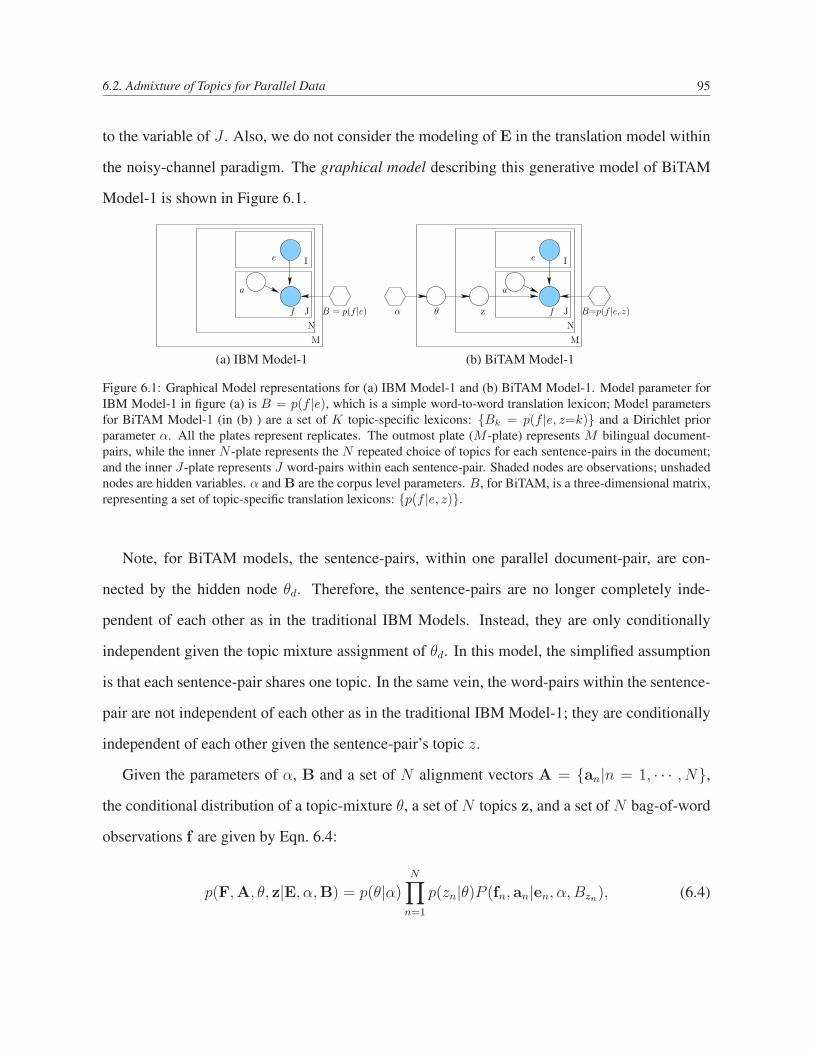
6.2. Admixture of Topics for Parallel Data 95
to the variable of J . Also, we do not consider the modeling of E in the translation model within
the noisy-channel paradigm. The graphical model describing this generative model of BiTAM
Model-1 is shown in Figure 6.1.
f J
I
N
e
a
M
B = p(f |e) f
a
J
I
N
M
e
θ zα B=p(f |e, z)
(a) IBM Model-1 (b) BiTAM Model-1
Figure 6.1: Graphical Model representations for (a) IBM Model-1 and (b) BiTAM Model-1. Model parameter forIBM Model-1 in figure (a) is B = p(f |e), which is a simple word-to-word translation lexicon; Model parametersfor BiTAM Model-1 (in (b) ) are a set of K topic-specific lexicons: {Bk = p(f |e, z=k)} and a Dirichlet priorparameter α. All the plates represent replicates. The outmost plate (M -plate) represents M bilingual document-pairs, while the inner N -plate represents the N repeated choice of topics for each sentence-pairs in the document;and the inner J-plate represents J word-pairs within each sentence-pair. Shaded nodes are observations; unshadednodes are hidden variables. α and B are the corpus level parameters. B, for BiTAM, is a three-dimensional matrix,representing a set of topic-specific translation lexicons: {p(f |e, z)}.
Note, for BiTAM models, the sentence-pairs, within one parallel document-pair, are con-
nected by the hidden node θd. Therefore, the sentence-pairs are no longer completely inde-
pendent of each other as in the traditional IBM Models. Instead, they are only conditionally
independent given the topic mixture assignment of θd. In this model, the simplified assumption
is that each sentence-pair shares one topic. In the same vein, the word-pairs within the sentence-
pair are not independent of each other as in the traditional IBM Model-1; they are conditionally
independent of each other given the sentence-pair’s topic z.
Given the parameters of α, B and a set of N alignment vectors A = {an|n = 1, · · · , N},
the conditional distribution of a topic-mixture θ, a set of N topics z, and a set of N bag-of-word
observations f are given by Eqn. 6.4:
p(F,A, θ, z|E, α,B) = p(θ|α)N∏
n=1
p(zn|θ)P (fn, an|en, α, Bzn), (6.4)

6.2. Admixture of Topics for Parallel Data 96
where p(zn|θ) = θi is the probability for sampling a topic z, such that zin = 1, where i is a unique
topic index. Marginalizing out θ and z, we can obtain the marginal distribution of generating F
from E for each parallel document-pair, as shown in Eqn. 6.5.
p(F,A|E, α,Bzn) =
∫p(θ|α)
(N∏
n=1
∑zn
p(zn|θ)p(fn, an|en,Bzn)
)dθ
=
∫p(θ|α)
(N∏
n=1
∑zn
p(zn|θ)p(fn|an, en,Bzn)p(an|en,Bzn)
)dθ(6.5)
where p(fn|en, an,Bzn) is a topic-specific sentence-level translation model under the topic as-
signment of zn. After marginalizing out the hidden topic assignments z, we have:
p(fn|en, an, θ) =∑zn
p(zn|θ)p(fn|en, an,Bzn), (6.6)
where p(zn|θ) = θi is the topic-weight for choosing topic-i, and this reveals that the proposed
sentence-level alignment model is, in essence, an additive mixture of topic-specific translation
models.
According to the simplified model shown in Figure 6.1, the French words fj’s are condition-
ally independent of each other, the alignment variables aj’s are independent of other variables,
and furthermore we assume all alignments are equally probable for the sake of simplicity. Now
the probability distribution for each sentence-pair is further simplified in Eqn. 6.7.
p(fn, an|en,Bzn) = p(fn|en, an,Bzn)p(an|en,Bzn)
≈ p(fn|en, an,Bzn)p(an)
=1
IJ
J∏j=1
p(fj|eaj,Bzn). (6.7)

6.2. Admixture of Topics for Parallel Data 97
The translation model for the whole parallel corpus is given by taking the product of the marginal
probabilities of each single document as in Eqn. 6.8.
P (CF ,CA|CE, α,B) =M∏
d=1
∫p(θd|α)
(Nd∏n=1
∑zdn
p(zdn|θ)p(fdn, adn|edn,Bzdn)
)dθd
∝M∏
d=1
∫p(θd|α)
(Nd∏n=1
∑zdn
p(zdn|θ) 1
IJdndn
Jdn∏j=1
p(fdnj|eadnj,Bzdn
)
)dθd.(6.8)
Finally, after we marginalize out the hidden alignment variable A, we can get the document-
level translation model as shown below:
P (CF |CE, α,B) =∑
{CA}
M∏
d=1
∫p(θd|α)
(Nd∏n=1
∑zdn
p(zdn|θ)Jdn∏j=1
p(fdn, adn|edn,Bzdn)
)dθd. (6.9)
Overall, in this generative model, the model parameters work at different-levels. The param-
eters of α and B are corpus-level parameters; θd is the document-level parameter, sampled once
per document-pair; the variable zdn is the sentence-level parameter, sampled once per sentence-
pair in the document-pair; the variables of fdnj and adnj are word-pair level variables, sampled
for each word-pair in the sentence-pair.
6.2.3 Inference and Learning for BiTAM Model-1
For inference and learning, the posterior distribution of the hidden variables given a document-
pair is shown in Eqn. 6.10.
p(A, θ, z|F,E, α,B) =p(F,A, θ, z|E, α,B)
p(F|E, α,B). (6.10)
Due to the hybrid nature of the “V” structure (explain-away structure) in the graphical model
in Figure 6.1, the hidden variables of A, θ, and z are all coupled together. This makes the joint
posterior distribution intractable to compute. We resort to the generalized mean field approxima-
tion as in Xing et al. (2003), and carry out the variational inference. The variational inference is
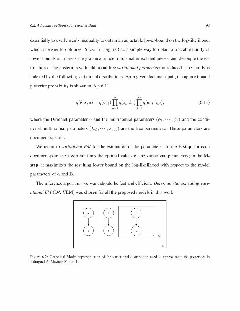
6.2. Admixture of Topics for Parallel Data 98
essentially to use Jensen’s inequality to obtain an adjustable lower-bound on the log-likelihood,
which is easier to optimize. Shown in Figure 6.2, a simple way to obtain a tractable family of
lower bounds is to break the graphical model into smaller isolated pieces, and decouple the es-
timation of the posteriors with additional free variational parameters introduced. The family is
indexed by the following variational distributions. For a given document-pair, the approximated
posterior probability is shown in Eqn.6.11.
q(θ, z, a) = q(θ|γ)N∏
n=1
q(zn|φn)Jn∏j=1
q(anj|λnj), (6.11)
where the Dirichlet parameter γ and the multinomial parameters (φ1, · · · , φn) and the condi-
tional multinomial parameters (λn1, · · · , λnJn) are the free parameters. These parameters are
document-specific.
We resort to variational EM for the estimation of the parameters. In the E-step, for each
document-pair, the algorithm finds the optimal values of the variational parameters; in the M-
step, it maximizes the resulting lower bound on the log-likelihood with respect to the model
parameters of α and B.
The inference algorithm we want should be fast and efficient. Deterministic annealing vari-
ational EM (DA-VEM) was chosen for all the proposed models in this work.
Figure 6.2: Graphical Model representation of the variational distribution used to approximate the posteriors inBilingual AdMixture Model-1.
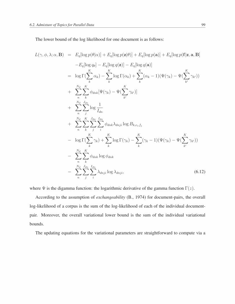
6.2. Admixture of Topics for Parallel Data 99
The lower bound of the log likelihood for one document is as follows:
L(γ, φ, λ; α,B) = Eq[log p(θ|α)] + Eq[log p(z|θ)] + Eq[log p(a)] + Eq[log p(f |z, a,B]
−Eq[log qθ]− Eq[log q(z)]− Eq[log q(a)]
= log Γ(K∑
k
αk)−K∑
k
log Γ(αk) +K∑
k
(αk − 1)(Ψ(γk)−Ψ(K∑
k′γk′))
+
Nd∑n
K∑
k
φdnk[Ψ(γk)−Ψ(K∑
k′γk′)]
+
Nd∑n
Jdn∑j
log1
Idn
+
Nd∑n
K∑
k
Jdn∑j
Idn∑i
φdnkλdnji log Bk,ei,fj
− log Γ(K∑
k
γk) +K∑
k
log Γ(γk)−K∑
k
(γk − 1)(Ψ(γk)−Ψ(K∑
k′γk′))
−Nd∑n
K∑
k
φdnk log φdnk
−Nd∑n
Jdn∑j
Idn∑i
λdnji log λdnji, (6.12)
where Ψ is the digamma function: the logarithmic derivative of the gamma function Γ(z).
According to the assumption of exchangeability (B., 1974) for document-pairs, the overall
log-likelihood of a corpus is the sum of the log-likelihood of each of the individual document-
pair. Moreover, the overall variational lower bound is the sum of the individual variational
bounds.
The updating equations for the variational parameters are straightforward to compute via a
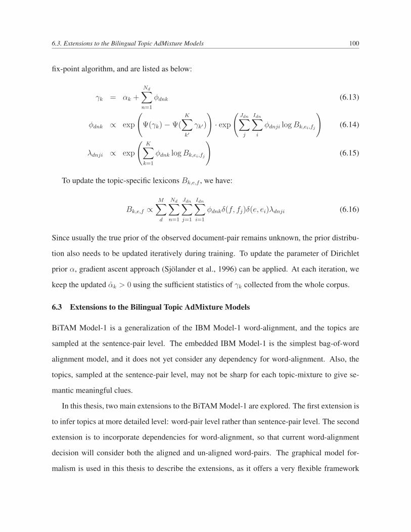
6.3. Extensions to the Bilingual Topic AdMixture Models 100
fix-point algorithm, and are listed as below:
γk = αk +
Nd∑n=1
φdnk (6.13)
φdnk ∝ exp
(Ψ(γk)−Ψ(
K∑
k′γk′)
)· exp
(Jdn∑j
Idn∑i
φdnji log Bk,ei,fj
)(6.14)
λdnji ∝ exp
(K∑
k=1
φdnk log Bk,ei,fj
)(6.15)
To update the topic-specific lexicons Bk,e,f , we have:
Bk,e,f ∝M∑
d
Nd∑n=1
Jdn∑j=1
Idn∑i=1
φdnkδ(f, fj)δ(e, ei)λdnji (6.16)
Since usually the true prior of the observed document-pair remains unknown, the prior distribu-
tion also needs to be updated iteratively during training. To update the parameter of Dirichlet
prior α, gradient ascent approach (Sjolander et al., 1996) can be applied. At each iteration, we
keep the updated αk > 0 using the sufficient statistics of γk collected from the whole corpus.
6.3 Extensions to the Bilingual Topic AdMixture Models
BiTAM Model-1 is a generalization of the IBM Model-1 word-alignment, and the topics are
sampled at the sentence-pair level. The embedded IBM Model-1 is the simplest bag-of-word
alignment model, and it does not yet consider any dependency for word-alignment. Also, the
topics, sampled at the sentence-pair level, may not be sharp for each topic-mixture to give se-
mantic meaningful clues.
In this thesis, two main extensions to the BiTAM Model-1 are explored. The first extension is
to infer topics at more detailed level: word-pair level rather than sentence-pair level. The second
extension is to incorporate dependencies for word-alignment, so that current word-alignment
decision will consider both the aligned and un-aligned word-pairs. The graphical model for-
malism is used in this thesis to describe the extensions, as it offers a very flexible framework
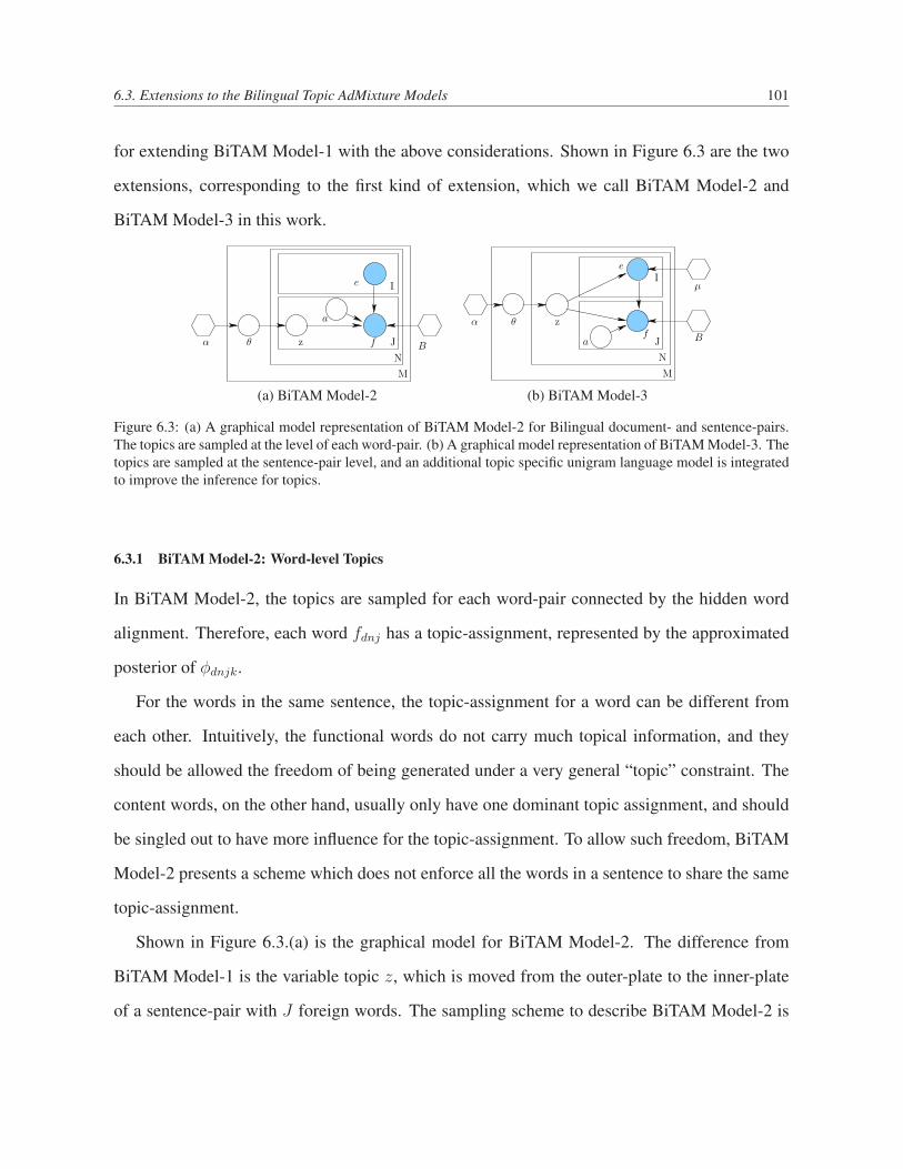
6.3. Extensions to the Bilingual Topic AdMixture Models 101
for extending BiTAM Model-1 with the above considerations. Shown in Figure 6.3 are the two
extensions, corresponding to the first kind of extension, which we call BiTAM Model-2 and
BiTAM Model-3 in this work.
a
J
I
N
M
e
Bθ zα f
µ
JB
I
f
e
a
α θ z
M
N
(a) BiTAM Model-2 (b) BiTAM Model-3
Figure 6.3: (a) A graphical model representation of BiTAM Model-2 for Bilingual document- and sentence-pairs.The topics are sampled at the level of each word-pair. (b) A graphical model representation of BiTAM Model-3. Thetopics are sampled at the sentence-pair level, and an additional topic specific unigram language model is integratedto improve the inference for topics.
6.3.1 BiTAM Model-2: Word-level Topics
In BiTAM Model-2, the topics are sampled for each word-pair connected by the hidden word
alignment. Therefore, each word fdnj has a topic-assignment, represented by the approximated
posterior of φdnjk.
For the words in the same sentence, the topic-assignment for a word can be different from
each other. Intuitively, the functional words do not carry much topical information, and they
should be allowed the freedom of being generated under a very general “topic” constraint. The
content words, on the other hand, usually only have one dominant topic assignment, and should
be singled out to have more influence for the topic-assignment. To allow such freedom, BiTAM
Model-2 presents a scheme which does not enforce all the words in a sentence to share the same
topic-assignment.
Shown in Figure 6.3.(a) is the graphical model for BiTAM Model-2. The difference from
BiTAM Model-1 is the variable topic z, which is moved from the outer-plate to the inner-plate
of a sentence-pair with J foreign words. The sampling scheme to describe BiTAM Model-2 is
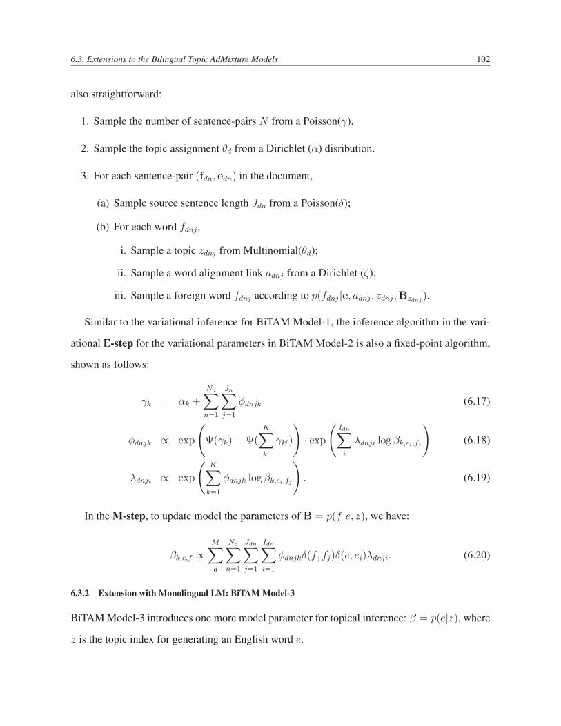
6.3. Extensions to the Bilingual Topic AdMixture Models 102
also straightforward:
1. Sample the number of sentence-pairs N from a Poisson(γ).
2. Sample the topic assignment θd from a Dirichlet (α) disribution.
3. For each sentence-pair (fdn, edn) in the document,
(a) Sample source sentence length Jdn from a Poisson(δ);
(b) For each word fdnj ,
i. Sample a topic zdnj from Multinomial(θd);
ii. Sample a word alignment link adnj from a Dirichlet (ζ);
iii. Sample a foreign word fdnj according to p(fdnj|e, adnj, zdnj,Bzdnj).
Similar to the variational inference for BiTAM Model-1, the inference algorithm in the vari-
ational E-step for the variational parameters in BiTAM Model-2 is also a fixed-point algorithm,
shown as follows:
γk = αk +
Nd∑n=1
Jn∑j=1
φdnjk (6.17)
φdnjk ∝ exp
(Ψ(γk)−Ψ(
K∑
k′γk′)
)· exp
(Idn∑i
λdnji log βk,ei,fj
)(6.18)
λdnji ∝ exp
(K∑
k=1
φdnjk log βk,ei,fj
). (6.19)
In the M-step, to update model the parameters of B = p(f |e, z), we have:
βk,e,f ∝M∑
d
Nd∑n=1
Jdn∑j=1
Idn∑i=1
φdnjkδ(f, fj)δ(e, ei)λdnji. (6.20)
6.3.2 Extension with Monolingual LM: BiTAM Model-3
BiTAM Model-3 introduces one more model parameter for topical inference: β = p(e|z), where
z is the topic index for generating an English word e.
6.3. Extensions to the Bilingual Topic AdMixture Models 103
Note that the likelihood we are optimizing is not the conditional-likelihood as in BiTAM
Model-1 and BiTAM Model-2. For BiTAM Model-3, we are optimizing the joint likelihood of
generating a document-pair (F,E). However, this joint likelihood can be decomposed into the
conditional likelihood part, as we do in the translation model , and the monolingual likelihood
part for generating the English document E, shown as in Eqn. 6.21.
P (F,E) = P (F|E)P (E). (6.21)
BiTAM Model-3 is generating both the target side E and the source side F of the parallel data:
for the bilingual part (f, e), we use the embedded topic-specific bilingual model: B = p(f |e, z),
and for the target side e ∈ E, we use a topic-specific monolingual unigram language model:
β = p(e|z). The two generative process are connected by the word-alignment variable a.
1. Sample the number of sentence-pairs N from a Poisson(γ),
2. Sample the topic assignment θd from a Dirichlet (α) prior,
3. For each sentence-pair (fdn, edn) in the document,
(a) Sample source sentence length Jdn from a Poisson(δ);
(b) Sample a topic zdn from Multinomial(θd);
(c) For each word fdnj ,
i. Sample a English word edni from a monolingual topic-specific language model
βzdn;
ii. Sample a word alignment link adnj = i from a Dirichlet (ζ);
iii. Sample a foreign word fdnj according to p(fdnj|e, adnj, zdnj,Bzdnj).
Similar to the inference for the BiTAM Model-1, the inference algorithm for the variational
6.4. HM-BiTAM: Extensions along the “A-chain” 104
parameters in BiTAM Model-3 is as follows:
γk = αk +
Nd∑n=1
φdnk (6.22)
φdnk ∝ exp
(Ψ(γk)−Ψ(
K∑
k′γk′)
)· exp
(N∑
n=1
Idn∑i
λdnji log Bk,fj ,ei
)
· exp
(N∑
n=1
Jdn∑j
Idn∑i
λdnji log βk,ei
)(6.23)
λdnji ∝ exp
(K∑
k=1
φdnk log Bk,ei,fj
)· exp
(K∑
k=1
φdnk log βk,ei
), (6.24)
where β serves as the smoothing parameter for updating the approximated posterior of φdnjk. It is
obvious that the newly introduced topic specific ungram language model β = p(e|z) influences
the word-alignment decisions of λdnji in Eqn. 6.24.
Similar to the BiTAM Model-1, to update the model parameters of B = p(f |e, z), we have:
Bk,e,f ∝M∑
d
Nd∑n=1
Jdn∑j=1
Idn∑i=1
φdnkδ(f, fj)δ(e, ei)λdnji. (6.25)
To update the model parameters of β = p(e|z), we have:
βk,e ∝M∑
d
Nd∑n=1
Jdn∑j=1
Idn∑i=1
δ(e, ei)φdnkλdnji. (6.26)
6.4 HM-BiTAM: Extensions along the “A-chain”
In Section 6.2.1, the Admixture model is illustrated with a basic alignment model: IBM Model-
1, which is a simple word-to-word level translation lexicon.
To date, hidden Markov models (HMMs) (Vogel et al., 1996) have been effectively used
in SMT. They are scalable to large training corpora, and are successfully used to boost higher-
order IBM models (Och and Ney, 2003). However, an HMM only generates words at each state
according to a word-based translation lexicon without considering the topical correlations among
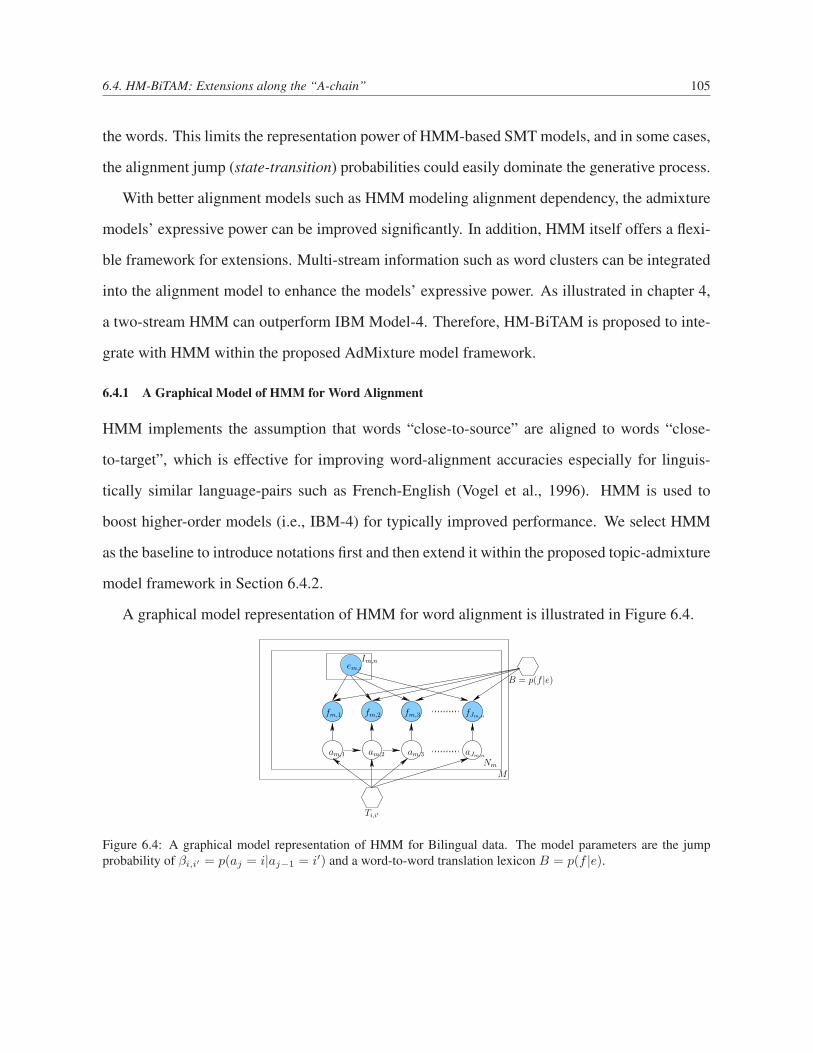
6.4. HM-BiTAM: Extensions along the “A-chain” 105
the words. This limits the representation power of HMM-based SMT models, and in some cases,
the alignment jump (state-transition) probabilities could easily dominate the generative process.
With better alignment models such as HMM modeling alignment dependency, the admixture
models’ expressive power can be improved significantly. In addition, HMM itself offers a flexi-
ble framework for extensions. Multi-stream information such as word clusters can be integrated
into the alignment model to enhance the models’ expressive power. As illustrated in chapter 4,
a two-stream HMM can outperform IBM Model-4. Therefore, HM-BiTAM is proposed to inte-
grate with HMM within the proposed AdMixture model framework.
6.4.1 A Graphical Model of HMM for Word Alignment
HMM implements the assumption that words “close-to-source” are aligned to words “close-
to-target”, which is effective for improving word-alignment accuracies especially for linguis-
tically similar language-pairs such as French-English (Vogel et al., 1996). HMM is used to
boost higher-order models (i.e., IBM-4) for typically improved performance. We select HMM
as the baseline to introduce notations first and then extend it within the proposed topic-admixture
model framework in Section 6.4.2.
A graphical model representation of HMM for word alignment is illustrated in Figure 6.4.
Ti,i′
fm,3fm,2fm,1 fJm,n
M
am,3am,2am,1 aJm,n
em,i
Im,n
B = p(f |e)
Nm
Figure 6.4: A graphical model representation of HMM for Bilingual data. The model parameters are the jumpprobability of βi,i′ = p(aj = i|aj−1 = i′) and a word-to-word translation lexicon B = p(f |e).

6.4. HM-BiTAM: Extensions along the “A-chain” 106
6.4.2 From HMM to HM-BiTAM
Instead of modeling parallel data as a bag of independent sentence-pairs in traditional IBM
models, we work directly on parallel document-pairs (F,E), which contain, for simplicity, N
one-to-one sentence-pair alignments (en, fn). The document-pair boundaries serve as the infor-
mative knowledge for inferring the topics of the sentence-pairs or word-pairs (ein , fjn) inside
of the document-pair. Similar to the previously introduced BiTAM models, a graphical model
representation of HM-BiTAM will be presented, and then the configuration of the embedded
HMM will be explained for alignment.
βi,i′
znθmα
f3f2f1
B
fJn
Nm
M
a3a2a1 aJn
ei
In
Figure 6.5: A graphical model representation of HM-BiTAM for Bilingual document- and sentence-pairs. A node inthe graph represents a random variable, and a hexagon denotes a parameter. Un-shaded nodes are hidden variables.The square boxes are “plates” that represent replicates of variables in the boxes. The outmost plate (M -plate)represents M bilingual document-pairs, while the inner N -plate represents the Nm sentences (each with its owntopic z) in, say, document m. The innermost I-plate represents the In words of the source sentence (i.e., the lengthof the English sentence).
6.4.3 Sampling Scheme for HM-BiTAM Model-1
Under a hidden Markov bilingual topic-admixture model, given a conjugate prior (which can be
either learned according to a maximum likelihood principle or empirically specified), the topic-
weight vector θn for each document-pair (Fn,En), is sampled independently; given θn and a
collection of topic-specific translation lexicons B, the sentence-pairs within (Fn,En) are drawn
independently from a mixture of topics. Following is an outline of the HM-BiTAM generative

6.4. HM-BiTAM: Extensions along the “A-chain” 107
process for each document-pair, indexed by n=1 · · ·M :
1. Sample N from a Poisson(γ).
2. Sample θn from a Dirichlet prior with parameter α.
3. For each sentence-pair (fn, en),
(a) Sample sentence length Nn from a Poisson(δ),
(b) Sample a topic zn from Multinomial(θn).
(c) For each position jn = 1, . . . , Jn in fn,
i. Sample an alignment link ajn from a first-order Markov dependency distribution:
p(ajn|ajn−1, β),
ii. Sample a foreign word fjn according to a topic-specific translation lexicon:
p(fjn|en, ajn , zn,B).
Similar to the BiTAM models introduced before, we denote the model parameter B as a vector
of topic-specific translation lexicons. Bi,j,k=p(f=fj|e=ei, z=k) is to translate e into f under a
given topic indexed by z. Parameter β is the jump-table, representing the transitions from aj−1 to
aj: βaj ,aj−1=p(aj|aj−1). Figure 6.5 shows a graphical model representation of the HM-BiTAM
generative process. Each sentence-pair is described with a random mixture of latent bilingual
topics, where each topic is associated with a distribution over bilingual word-pairs. Each word f
is assumed to have been generated by a latent topic z drawn from a document-specific distribu-
tion over K topics and the aligned English word e identified by the hidden alignment variable a.
A variational EM is designed to predict, for each sentence-pair within a document-pair, which
topics it belongs to. The proposed model is to infer the topic mixtures and the weights associated
with the topics in an unsupervised fashion.
6.4. HM-BiTAM: Extensions along the “A-chain” 108
6.4.4 First-order Markov Dependency for Alignment
The Markov dependency for word-alignment follows the scheme in Vogel et al. (1996), and we
have adopted a simple strategy to deal with the “NULL” word. “NULL” is a special word for
the source words which do not have translations in the target sentence. However, the position
of “NULL” is not well defined in the target sentence. This causes confusions in estimating the
transition probabilities involving jumping to or from a NULL word.
In this work, we assume NULL word moves freely within the target sentence. Therefore,
the jumping distances involving NULL are simplified to be position-difference. A more delicate
approach is in Toutanova et al. (2002); NULL is treated as the left-context of the current source
position, and it competes with the corresponding English words to generate the source word.
GIZA++ 1 introduces more dependencies into the transition table by including sentence length,
position, and word-classes. In this work, as the aim is not to enrich the transition structures, we
choose the simplest scheme for NULL. Shown in Figure 6.6, a pseudo position is then assigned
to be between every two adjacent positions in the target sentence for word NULL. Therefore,
the HMM parameters for transitions are reduced to two components: first, a zero-order jump-
distance for transitions involving NULL word, and second, for alignment jumps between two
real words, we use first-order Markov dependencies: p(aj|aj−1).
We initialize the transition matrix using the following scheme:
p(aj|aj−1) ∝
‖aj − aj−1‖−α, if aj 6= aj−1
1.0I
, if aj = aj−1
, (6.27)
where α can control the shape of the jump-table, such that the alignment focus more on short
jumping-distances and penalize more on no-jumps and long-jumps. In all the experiments, α
was set to 2.0. We initialize the zero-order transition involving NULL word to be uniformly
distributed as 1.0/I . In our empirical observations, the above configured jump-table is very1http://www.fjoch.com/GIZA++.html.
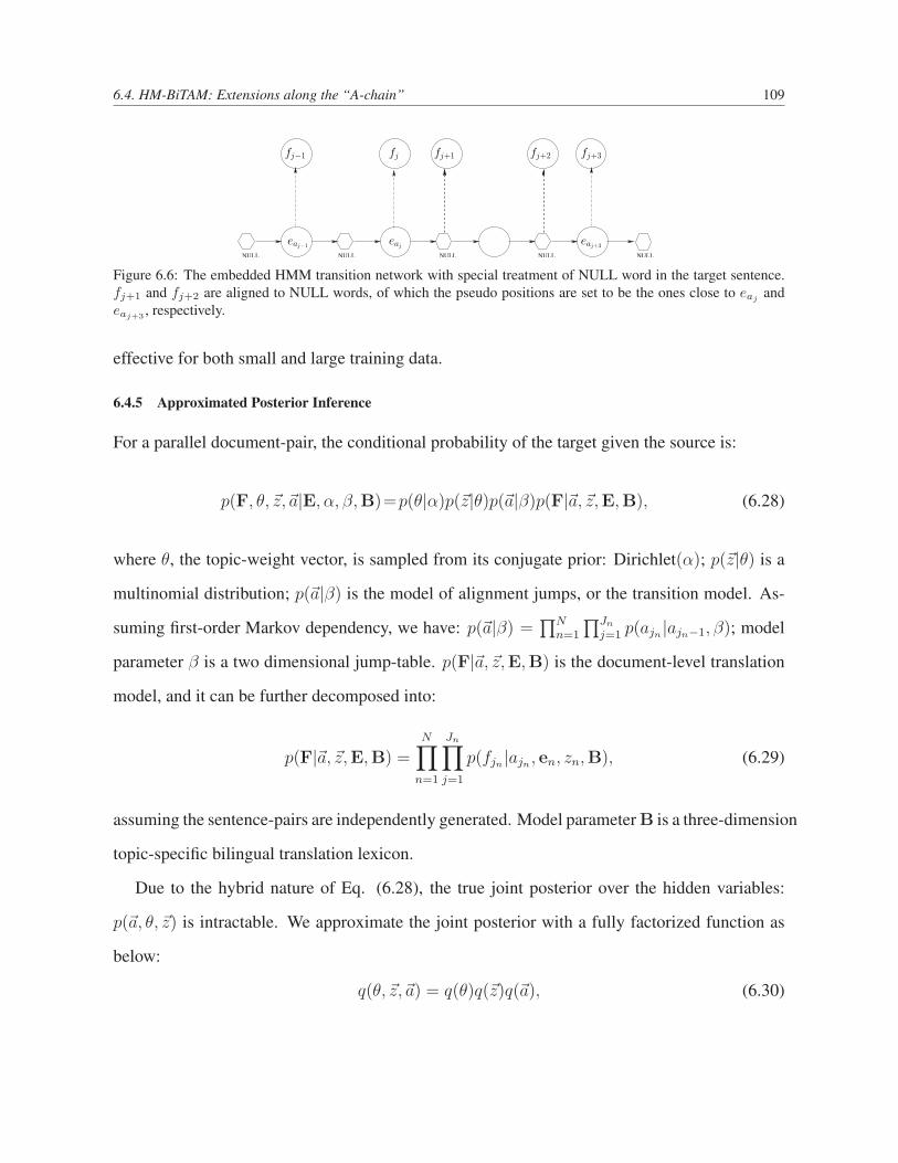
6.4. HM-BiTAM: Extensions along the “A-chain” 109
NULL NULL NULL NULLNULL
fj+1 fj+2 fj+3fj−1 fj
eaj−1eaj+3
eaj
Figure 6.6: The embedded HMM transition network with special treatment of NULL word in the target sentence.fj+1 and fj+2 are aligned to NULL words, of which the pseudo positions are set to be the ones close to eaj
andeaj+3 , respectively.
effective for both small and large training data.
6.4.5 Approximated Posterior Inference
For a parallel document-pair, the conditional probability of the target given the source is:
p(F, θ, ~z,~a|E, α, β,B)=p(θ|α)p(~z|θ)p(~a|β)p(F|~a, ~z,E,B), (6.28)
where θ, the topic-weight vector, is sampled from its conjugate prior: Dirichlet(α); p(~z|θ) is a
multinomial distribution; p(~a|β) is the model of alignment jumps, or the transition model. As-
suming first-order Markov dependency, we have: p(~a|β) =∏N
n=1
∏Jn
j=1 p(ajn|ajn−1, β); model
parameter β is a two dimensional jump-table. p(F|~a, ~z,E,B) is the document-level translation
model, and it can be further decomposed into:
p(F|~a, ~z,E,B) =N∏
n=1
Jn∏j=1
p(fjn|ajn , en, zn,B), (6.29)
assuming the sentence-pairs are independently generated. Model parameter B is a three-dimension
topic-specific bilingual translation lexicon.
Due to the hybrid nature of Eq. (6.28), the true joint posterior over the hidden variables:
p(~a, θ, ~z) is intractable. We approximate the joint posterior with a fully factorized function as
below:
q(θ, ~z,~a) = q(θ)q(~z)q(~a), (6.30)
6.4. HM-BiTAM: Extensions along the “A-chain” 110
where q(θ) is a Dirichlet distribution; q(~z) is a multinomial; and q(~a) follows a re-parameterized
HMM:
q(~θ|~γ) =Γ(
∑Kk=1)γk∏K
k=1 Γ(γk)·
K∏
k=1
θγk−1k (6.31)
q(~z|~φ) =N∏
n=1
K∏
k=1
φ1(zn,k)nk (6.32)
q(~a|~λ) =N∏
n=1
( Jn∏j=1
In∏i=1
λ1(ajn ,i)n,jn,in
Jn∏j=1
p(ajn|ajn−1)), (6.33)
where γk, φnk and λn,j,i are variational parameters, and 1(·, ·) is an equality indicator function.
Similar to the derivations as in Blei et al. (2003), by minimizing the Kullback-Leibler distance
between p(·) and q(·), it is equivalent to optimizing the lower-bound of the conditional likelihood
for the parallel data, :
L(~a, θ, ~z; β,B) = Eq{log(p(F, θ,~z,~a|E,α,β,B))}−Eq{log(q(θ,~z,~a))}, (6.34)
where Eq denotes the expectation with regard to the distribution of q(·). Because of the fully
factorized nature of q(·), the computations of these expectations are now tractable.
Variational EM (VEM) is a generalization of EM; it iterates between optimizing the vari-
ational parameters, and inferring the hidden variable distributions. The E-step in VEM is an
iterative fixed-point algorithm for updating the hidden variables. The updating equations are
6.4. HM-BiTAM: Extensions along the “A-chain” 111
shown as below:
γk = αk +N∑
n=1
φnk (6.35)
φnk ∝ exp(Ψ(γk)−Ψ(
K∑
k=1
γk))
× exp(Jn,In∑j,i=1
∑f∈VF
∑e∈VE
1(fjn , f)1(ein , e)λn,j,ilog Bf,e,k
)(6.36)
λn,j,i ∝ exp( In∑
i′=1
λn,j−1,i′ log βi,i′
)× exp
( In∑
i”=1
λn,j+1,i” log βi”,i
)
× exp(∑f∈VF
∑e∈VE
1(fjn ,f)1(ein ,e)K∑
k=1
φn,k log Bf,e,k
). (6.37)
Intuitively, the first two terms on the right side of the Eq. (6.37) represent the messages
corresponding to the forward and backward passes in HMM; the third term represents the state-
emission probabilities, which can be viewed as a geometric interpolation of the strengths of
individual topic-specific lexicons. The λn,j,i’s are the approximated posteriors of the alignment
in the proposed topic-specific HMM model. This approximated posterior, as shown in Eqn. 6.37,
is in essence an exponential model, combining three sets of feature functions: forward and
backward edge potentials, and the node potential for the weighted topic-specific lexicons.
The topic weight-vector {φnk} in Eq. (6.36) is associated with the topic mixtures for each
sentence-pair within a document-pair. It represents the approximate posteriors of the topic
weights for each sentence-pair (~fn, ~en). The topical information for updating {φnk} are col-
lected from the individual aligned word-pairs associated with the corresponding topic-specific
translation lexicon probabilities and smoothed by the priors from a Dirichlet distribution.
After the E-step converges for updating variational parameters in Eqn. 6.35-6.37, the maximal
likelihood updates of the transition matrix ~β and the translation lexicons B are carried out in M-
6.5. Extensions to HM-BiTAM: Topics Sampled at Word-pair Level 112
step as follows:
βi”,i′ ∝N∑
n=1
Jn∑j=1
λn,j,i”λn,j−1,i′ (6.38)
~Bf,e,k∝N∑
n=1
Jn∑j=1
In∑i=1
K∑k=1
1(fjn , f)1(ein , e)λn,j,iφn,k. (6.39)
For updating Dirichlet parameter α, the corpus-level parameter, we resort to gradient accent
(Sjolander et al., 1996). The overall computation complexity of the model is linear to the number
of topics.
6.5 Extensions to HM-BiTAM: Topics Sampled at Word-pair Level
Sentences, especially the long sentences, can usually correlated with more than one topics, while
word usually exemplify one topic. Intuitively, topics sampled at word-pair level are potentially
sharper than those sampled at sentence-pair level. The extension to BiTAM Model-1, encod-
ing more word-alignment dependencies for the parallel data, is already shown in HM-BiTAM
Model-1. Another extension to BiTAM Model-1 is to encode both word alignment dependency
the same as in HM-BiTAM Model-1, and it also samples topics at word-pair level. HM-BiTAM
Model-2 will be explained in this section with the two extended features. Given the graphical
model representation, the extensions become easy to construct, and the sampling scheme and
variational EM for HM-BiTAM Model-2 are straightforward to derive as shown in the follows.
6.5.1 HM-BiTAM Model-2
Shown in Figure 6.7 is HM-BiTAM Model-2. The topics are sampled at the word-pair level
instead of the sentence-pair level. The graphical model structure is close to the HM-BiTAM
Model-1, and the sampling scheme and variational EM are all very close.
6.5.2 Generative Scheme of HM-BiTAM Model-2
1. Sample N from a Poisson(γ).

6.5. Extensions to HM-BiTAM: Topics Sampled at Word-pair Level 113
B
Nm
M
aJn
βi,i′
a3a2a1
α
θm
f3
ei
In zn,1 zn,2 zn,3 zn,J
f2f1 fJn
Figure 6.7: A graphical model representation of HM-BiTAM Model-2 for Bilingual document- and sentence-pairs.The topics are sampled at the word-pair level instead of at sentence-pair level as in HM-BiTAM Model-1.
2. Sample θn from a Dirichlet prior with parameter α.
3. For each sentence-pair (fn, en),
(a) Sample sentence length Nn from a Poisson(δ),
(b) For each position jn = 1, . . . , Jn in fn,
i. Sample a topic znj from Multinomial(θn).
ii. Sample an alignment link ajn from a first-order Markov dependency distribution:
p(ajn|ajn−1, β),
iii. Sample a foreign word fjn according to a topic-specific translation lexicon:
p(fjn|en, ajn , zn,j,B).
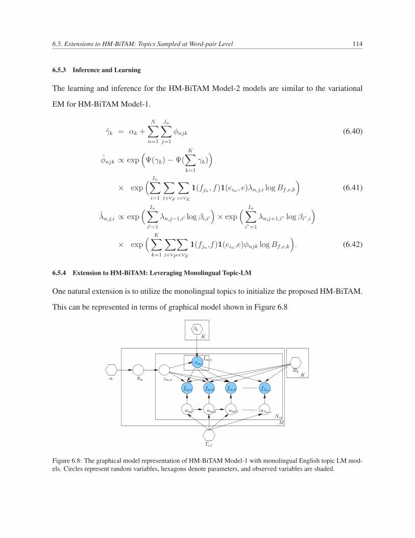
6.5. Extensions to HM-BiTAM: Topics Sampled at Word-pair Level 114
6.5.3 Inference and Learning
The learning and inference for the HM-BiTAM Model-2 models are similar to the variational
EM for HM-BiTAM Model-1.
γk = αk +N∑
n=1
Jn∑j=1
φnjk (6.40)
φnjk ∝ exp(Ψ(γk)−Ψ(
K∑
k=1
γk))
× exp( In∑
i=1
∑f∈VF
∑e∈VE
1(fjn , f)1(ein , e)λn,j,i log Bf,e,k
)(6.41)
λn,j,i ∝ exp( In∑
i′=1
λn,j−1,i′ log βi,i′
)× exp
( In∑
i”=1
λn,j+1,i” log βi”,i
)
× exp( K∑
k=1
∑f∈VF
∑e∈VE
1(fjn ,f)1(ein ,e)φnjk log Bf,e,k
). (6.42)
6.5.4 Extension to HM-BiTAM: Leveraging Monolingual Topic-LM
One natural extension is to utilize the monolingual topics to initialize the proposed HM-BiTAM.
This can be represented in terms of graphical model shown in Figure 6.8
α zm,nθm
fm,3fm,2fm,1
Bk
fJm,n
Nm
M
am,3am,2am,1
em,i
Im,n
Ti,i′
βk
K
K
aJm,n
Figure 6.8: The graphical model representation of HM-BiTAM Model-1 with monolingual English topic LM mod-els. Circles represent random variables, hexagons denote parameters, and observed variables are shaded.
6.5. Extensions to HM-BiTAM: Topics Sampled at Word-pair Level 115
In this way, the topical information from monolingual data (Here is English) will be propoa-
gated to update the topics for the parallel data. The sampling schem and the variational EM are
changed slightly. The modified variational EM is given here.
In the E-step, we have:
γk = αk +N∑
n=1
φn,k, (6.43)
φn,k ∝ exp(Ψ(γk)−Ψ(
K∑
k=1
γk))· exp
( In∑i=1
Jn∑j=1
λn,j,i log βk,ein
)
× exp(Jn,In∑j,i=1
∑f∈VF
∑e∈VE
1(fjn , f)1(ein , e)λn,j,ilog Bf,e,k
), (6.44)
λn,j,i ∝ exp( In∑
i′=1
λn,j−1,i′ log Ti,i′
)× exp
( In∑
i”=1
λn,j+1,i” log Ti”,i
)
× exp(∑f∈VF
∑e∈VE
1(fjn ,f)1(ein ,e)K∑
k=1
φn,k log Bf,e,k
)× exp
( K∑
k=1
φn,k log βk,ein
),(6.45)
where 1(·, ·) denotes an indicator function, and Ψ(·) represents the digamma function.
The vector φn ≡ (φn,1, . . . , φn,K) given by Eq. (6.44) represents the approximate posterior
of the topic weights for each sentence-pair (fn, en). The topical information for updating φn is
collected from three aspects: aligned word-pairs weighted by the corresponding topic-specific
translation lexicon probabilities, topical distributions of monolingual English language model,
and the smoothing factors from the topic prior.
Equation (6.45) gives the approximate posterior probability for alignment between the j-th
word in fn and the i-th word in en. Intuitively, the first two terms represent the messages corre-
sponding to the forward and backward passes in HMM; The third term represents the emission
probabilities, and it can be viewed as a geometric interpolation of the strengths of individual
topic-specific lexicons; and the last term provides further smoothing from monolingual topic-
specific aspects.
6.6. Inference of Word Alignment with BiTAMs 116
The update equations for the M-step are as below:
Ti”,i′ ∝N∑
n=1
Jn∑j=1
λn,j,i”λn,j−1,i′ , (6.46)
Bf,e,k∝N∑
n=1
Jn∑j=1
In∑i=1
K∑k=1
1(fjn , f)1(ein , e)λn,j,iφn,k, (6.47)
βk,e∝N∑
n=1
In∑i=1
Jn∑j=1
1ei,eλnjiφn,k. (6.48)
For updating Dirichlet hyperparameter α, which is a corpora-level parameter, we resort to gra-
dient accent (Sjolander et al., 1996). The overall computation complexity of the model is linear
to the number of topics.
6.6 Inference of Word Alignment with BiTAMs
We use the same Viterbi word-alignment retrieval algorithm as the one used in traditional IBM
Models and HMM for word-alignment.
The posterior mean of the alignment indicators ajn = i, captured by the so called the approx-
imated posterior alignment matrix λn,j,i. In Viterbi algorithm, we use a French word fjn (at the
j′th position of n′th sentence to query the row of λn,j,i to get the best aligned English word (by
taking the maximum point in a row:
ajn = arg maxi∈[1,In]
{λn,j,i
}. (6.49)
It only generates one aligned English word per source word (one-to-one). Since BiTAM
models are still noisy channel models, so we can use the same heuristics to symmetrize the word
alignments, as used with the IBM models for building phrase-based machine translation. The
heuristics include union, intersection, and Refined, which grow the intersection of the alignments
obtained from both directions of the noisy-channel models with additional aligned word-pairs
seen in the union.
6.7. Experiments 117
6.7 Experiments
In the experimental setup, we want to answer several questions:
• Can the proposed BiTAM models improve the likelihood of the unseen test data over the
traditional IBM Models 1 ∼ 4?
• What kinds of the hidden topics are learned with BiTAM models from parallel document-
pairs?
• Can BiTAM models improve the word alignment accuracy?
• Can BiTAM models improve the translation quality?
6.7.1 The Data
Most of the parallel sentences are from document-pairs which have certain logical concept flow.
The training data for the Admixture models is a collection of parallel document-pairs, as shown
in Table 6.1. To model the hidden concepts specific to document-pairs, it is necessary to have
the document boundaries of parallel data; however, the order of the parallel sentences is not
required to be the same as the original in the BiTAM models investigated here. Some of the
data sets provided by LDC and the data from European Union are qualified: the high quality
FBIS data, Sinorama data, Xinhua News, European Parliament Plenary Sessions (EPPS) and the
data from United Nations Debates. Most of the other data sets, however, are not suitable for
the BiTAM models’ training because the document-boundaries are missing. For instance, the
BTEC data is from phrase-books for tourism domain, and there is no document boundaries in
the data. Therefore, it is not suitable for the training of BiTAM models. Because not all the
parallel corpora provided by LDC contains document-boundary, the collected training data for
BiTAM models has up to 33K document-pairs, and around 22.6 million English words.
The parallel document-pairs can be mined using the full-text bilingual document alignment
models as described in Chapt. 3.2; and the parallel sentence-pairs can be obtained by the sentence-

6.7. Experiments 118
alignment models in Chapt. 3.3. The data set released under LDC2002E18 (Xinhua News data
in Table 6.1) is one such example.
Train #Doc. #Sent.#Tokens
English Chinese
TreeBank* 316 4172 133598 105331Sinorama05* 6367 282176 10321061 10027095Sinorama02* 2373 103252 3810664 3146014chnews.2005* 1001 10317 326347 270274FOUO * 15180 414266 17490921 13188097FBIS.BEIJING* 6111 99396 4199030 3527786XinHuaNewsStory* 17260 98444 3807884 3915267
Treebank 316 4172 133598 105331All 33,428 597,757 22,598,584 20,991,767
Table 6.1: Training and Test data statistics
The training data sets are mainly general newswire style text, covering topics like economics,
politics, and sports. Two training data sets were selected for experiments of two scenarios: the
small-data track and the large-data track.
The small-data track for Chinese-English statistical machine translation, from TIDES eval-
uation, aims to investigate close-to-optimal configurations for BiTAMs and HM-BiTAMs. The
training data is from the Chinese-Treebank. This is also to simulate the scenarios of low-density
language-pairs for machine translation. After document boundary detection1, tokenization, sen-
tence segmentations, and long sentences’ splitting., there are totally 280 document-pairs in the
small training data, containing 4127 parallel sentence pairs.
The large-data track is used to test the scalability and effectiveness for the proposed BiTAMs
and HM-BiTAMs. The large training data set has up to 33 K document-pairs. It is collected from
Treebank (LDC2002E17), FBIS (LDC2003E14), Sinorama05 (LDC2005T10), Sinorama02(LDC2002E58),
FOUO (LDC2006G05), FBIS (Beijing part) and ten-year Xinhua news story collection (LDC2002E18).
The large training data set is to simulate the scenarios of high-density language-pair resources
such as Arabic and Chinese. When the training data grows large, more hidden factors come
into play for modeling the translations. At the same time, large training data can also cover1Here, the newswire document ending marker “(end)” in the TreeBank data is used to classify document boundaries.
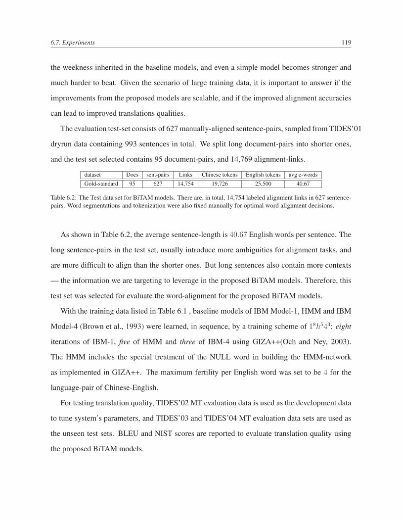
6.7. Experiments 119
the weekness inherited in the baseline models, and even a simple model becomes stronger and
much harder to beat. Given the scenario of large training data, it is important to answer if the
improvements from the proposed models are scalable, and if the improved alignment accuracies
can lead to improved translations qualities.
The evaluation test-set consists of 627 manually-aligned sentence-pairs, sampled from TIDES’01
dryrun data containing 993 sentences in total. We split long document-pairs into shorter ones,
and the test set selected contains 95 document-pairs, and 14,769 alignment-links.
dataset Docs sent-pairs Links Chinese tokens English tokens avg e-words
Gold-standard 95 627 14,754 19,726 25,500 40.67
Table 6.2: The Test data set for BiTAM models. There are, in total, 14,754 labeled alignment links in 627 sentence-pairs. Word segmentations and tokenization were also fixed manually for optimal word alignment decisions.
As shown in Table 6.2, the average sentence-length is 40.67 English words per sentence. The
long sentence-pairs in the test set, usually introduce more ambiguities for alignment tasks, and
are more difficult to align than the shorter ones. But long sentences also contain more contexts
— the information we are targeting to leverage in the proposed BiTAM models. Therefore, this
test set was selected for evaluate the word-alignment for the proposed BiTAM models.
With the training data listed in Table 6.1 , baseline models of IBM Model-1, HMM and IBM
Model-4 (Brown et al., 1993) were learned, in sequence, by a training scheme of 18h543: eight
iterations of IBM-1, five of HMM and three of IBM-4 using GIZA++(Och and Ney, 2003).
The HMM includes the special treatment of the NULL word in building the HMM-network
as implemented in GIZA++. The maximum fertility per English word was set to be 4 for the
language-pair of Chinese-English.
For testing translation quality, TIDES’02 MT evaluation data is used as the development data
to tune system’s parameters, and TIDES’03 and TIDES’04 MT evaluation data sets are used as
the unseen test sets. BLEU and NIST scores are reported to evaluate translation quality using
the proposed BiTAM models.
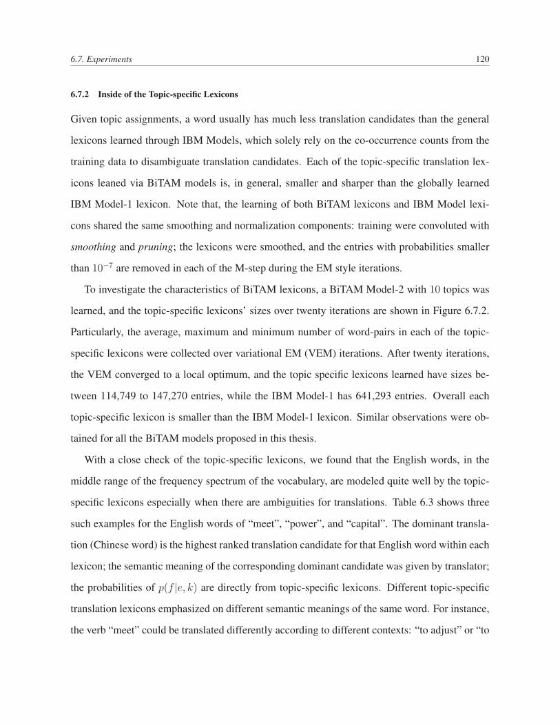
6.7. Experiments 120
6.7.2 Inside of the Topic-specific Lexicons
Given topic assignments, a word usually has much less translation candidates than the general
lexicons learned through IBM Models, which solely rely on the co-occurrence counts from the
training data to disambiguate translation candidates. Each of the topic-specific translation lex-
icons leaned via BiTAM models is, in general, smaller and sharper than the globally learned
IBM Model-1 lexicon. Note that, the learning of both BiTAM lexicons and IBM Model lexi-
cons shared the same smoothing and normalization components: training were convoluted with
smoothing and pruning; the lexicons were smoothed, and the entries with probabilities smaller
than 10−7 are removed in each of the M-step during the EM style iterations.
To investigate the characteristics of BiTAM lexicons, a BiTAM Model-2 with 10 topics was
learned, and the topic-specific lexicons’ sizes over twenty iterations are shown in Figure 6.7.2.
Particularly, the average, maximum and minimum number of word-pairs in each of the topic-
specific lexicons were collected over variational EM (VEM) iterations. After twenty iterations,
the VEM converged to a local optimum, and the topic specific lexicons learned have sizes be-
tween 114,749 to 147,270 entries, while the IBM Model-1 has 641,293 entries. Overall each
topic-specific lexicon is smaller than the IBM Model-1 lexicon. Similar observations were ob-
tained for all the BiTAM models proposed in this thesis.
With a close check of the topic-specific lexicons, we found that the English words, in the
middle range of the frequency spectrum of the vocabulary, are modeled quite well by the topic-
specific lexicons especially when there are ambiguities for translations. Table 6.3 shows three
such examples for the English words of “meet”, “power”, and “capital”. The dominant transla-
tion (Chinese word) is the highest ranked translation candidate for that English word within each
lexicon; the semantic meaning of the corresponding dominant candidate was given by translator;
the probabilities of p(f |e, k) are directly from topic-specific lexicons. Different topic-specific
translation lexicons emphasized on different semantic meanings of the same word. For instance,
the verb “meet” could be translated differently according to different contexts: “to adjust” or “to
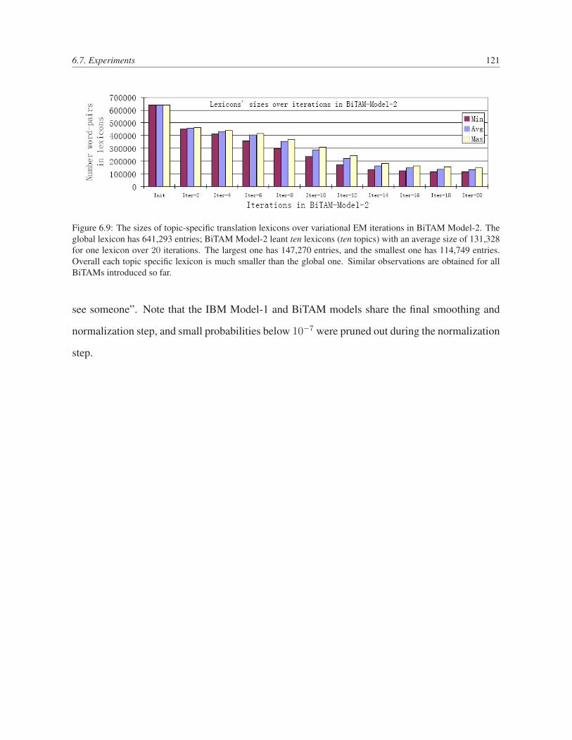
6.7. Experiments 121
Figure 6.9: The sizes of topic-specific translation lexicons over variational EM iterations in BiTAM Model-2. Theglobal lexicon has 641,293 entries; BiTAM Model-2 leant ten lexicons (ten topics) with an average size of 131,328for one lexicon over 20 iterations. The largest one has 147,270 entries, and the smallest one has 114,749 entries.Overall each topic specific lexicon is much smaller than the global one. Similar observations are obtained for allBiTAMs introduced so far.
see someone”. Note that the IBM Model-1 and BiTAM models share the final smoothing and
normalization step, and small probabilities below 10−7 were pruned out during the normalization
step.
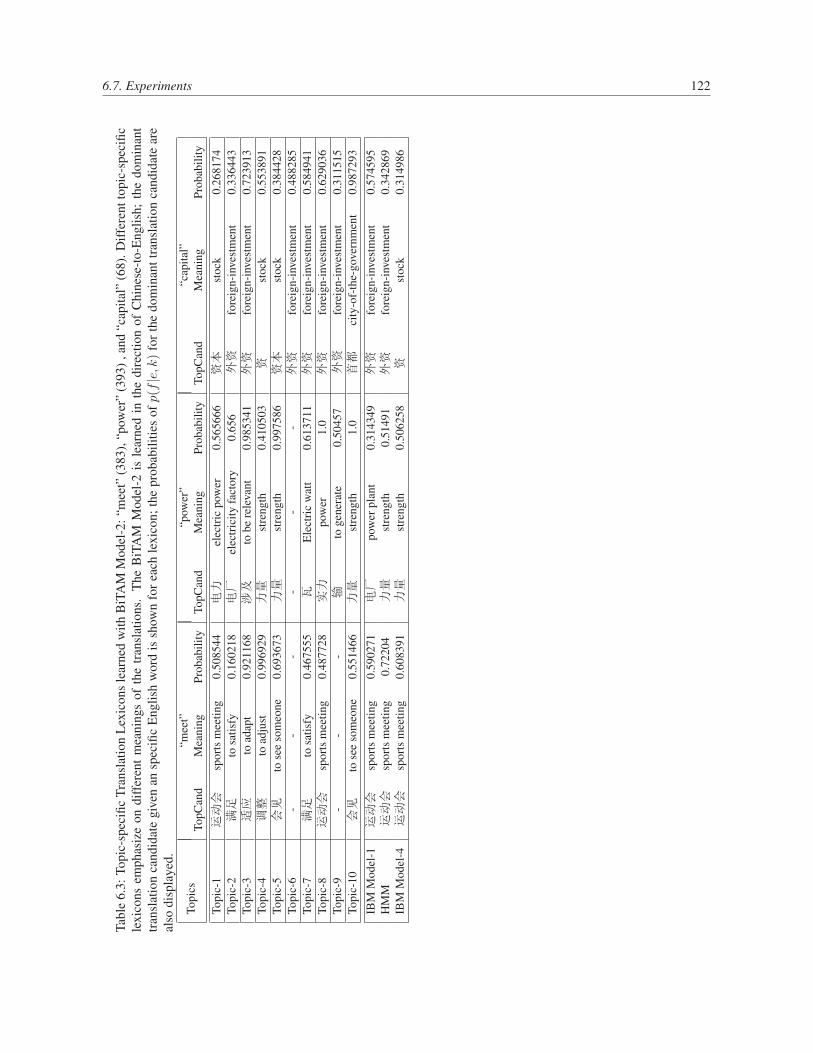
6.7. Experiments 122
Tabl
e6.
3:To
pic-
spec
ific
Tran
slat
ion
Lex
icon
sle
arne
dw
ithB
iTA
MM
odel
-2:“
mee
t”(3
83),
“pow
er”
(393
),an
d“c
apita
l”(6
8).D
iffer
entt
opic
-spe
cific
lexi
cons
emph
asiz
eon
diff
eren
tm
eani
ngs
ofth
etr
ansl
atio
ns.
The
BiT
AM
Mod
el-2
isle
arne
din
the
dire
ctio
nof
Chi
nese
-to-
Eng
lish;
the
dom
inan
ttr
ansl
atio
nca
ndid
ate
give
nan
spec
ific
Eng
lish
wor
dis
show
nfo
rea
chle
xico
n;th
epr
obab
ilitie
sof
p(f|e,
k)
for
the
dom
inan
ttra
nsla
tion
cand
idat
ear
eal
sodi
spla
yed.
Topi
cs“m
eet”
“pow
er”
“cap
ital”
TopC
and
Mea
ning
Prob
abili
tyTo
pCan
dM
eani
ngPr
obab
ility
TopC
and
Mea
ning
Prob
abili
ty
Topi
c-1
运动会
spor
tsm
eetin
g0.
5085
44电力
elec
tric
pow
er0.
5656
66资本
stoc
k0.
2681
74To
pic-
2满足
tosa
tisfy
0.16
0218
电厂
elec
tric
ityfa
ctor
y0.
656
外资
fore
ign-
inve
stm
ent
0.33
6443
Topi
c-3
适应
toad
apt
0.92
1168
涉及
tobe
rele
vant
0.98
5341
外资
fore
ign-
inve
stm
ent
0.72
3913
Topi
c-4
调整
toad
just
0.99
6929
力量
stre
ngth
0.41
0503
资st
ock
0.55
3891
Topi
c-5
会见
tose
eso
meo
ne0.
6936
73力量
stre
ngth
0.99
7586
资本
stoc
k0.
3844
28To
pic-
6-
--
--
-外资
fore
ign-
inve
stm
ent
0.48
8285
Topi
c-7
满足
tosa
tisfy
0.46
7555
瓦E
lect
ric
wat
t0.
6137
11外资
fore
ign-
inve
stm
ent
0.58
4941
Topi
c-8
运动会
spor
tsm
eetin
g0.
4877
28实力
pow
er1.
0外资
fore
ign-
inve
stm
ent
0.62
9036
Topi
c-9
--
-输
toge
nera
te0.
5045
7外资
fore
ign-
inve
stm
ent
0.31
1515
Topi
c-10
会见
tose
eso
meo
ne0.
5514
66力量
stre
ngth
1.0
首都
city
-of-
the-
gove
rnm
ent
0.98
7293
IBM
Mod
el-1
运动会
spor
tsm
eetin
g0.
5902
71电厂
pow
erpl
ant
0.31
4349
外资
fore
ign-
inve
stm
ent
0.57
4595
HM
M运动会
spor
tsm
eetin
g0.
7220
4力量
stre
ngth
0.51
491
外资
fore
ign-
inve
stm
ent
0.34
2869
IBM
Mod
el-4
运动会
spor
tsm
eetin
g0.
6083
91力量
stre
ngth
0.50
6258
资st
ock
0.31
4986

6.7. Experiments 123
Table 6.4: Topic-specific Translation Lexicons p(e|f, k) learned from BiTAM Model-2 in the direction of English-to-Chinese. Different topic-specific lexicons from BiTAM, emphasize on different semantic meanings of the Chi-nese word for translations. The baseline IBM Model-1 lexicon proposes translation candidates solely based onco-occurrence statistics from training data; BiTAM models propose various candidates according to underlyingtopics inferred from the data. The high frequent words can dominate both IBM and BiTAM models. However,BiTAM models are relatively less polluted.
Topics分 台 港
TopCand p(e|f, k) TopCand p(e|f, k) TopCand p(e|f, k)
Topic-1 part 0.356084 sets 0.36889 port 0.339554Topic-2 component 0.336602 from 0.619634 port 0.916524Topic-3 portion 0.636405 taiwan 0.325529 the 0.769986Topic-4 score 0.199637 of 0.512724 kong 0.437063Topic-5 components 0.424127 taiwan 0.49379 port 0.218575Topic-6 drafting 1.0 sets 0.709279 port 0.112944Topic-7 points 0.489062 and 0.438952 hong 0.119163Topic-8 portion 1.0 parts 0.344728 kong 0.31599Topic-9 minutes 0.948216 taiwan 0.368632 the 0.519904Topic-10 component 0.646592 taiwan 0.461473 port 0.573701
IBM Model-1 the 0.250177 and 0.311071 port 0.290295HMM of 0.319917 taiwan 0.308263 port 0.424215IBM Model-4 of 0.502472 taiwan 0.342031 port 0.359474
One can usually find some topic-specific trends in the learned topic-specific lexicons using
BiTAM models. One example, as shown in Table 6.5, is the translation of the English word “Ko-
rean”. The word “North Korean”, in the newswire corpus, co-occurring with politics and nuclear
weapons, and “North Korean” is translated into Chinese word “朝鲜” (Chao2 Xian3) 2; while
the “South Korean” co-occurred more with economics and development, and it is translated into
Chinese word “韩国”(Han2 Guo2), which does not share any Chinese characters with “朝鲜”
(Chao2 Xian3). Table 6.5 shows the BiTAM Model-1 learned with small training data. Within
each of them, “Korean” were queried with its best translations in each topic-specific lexicon. In
the resultant lexicons from BiTAM Model-1 with ten topics, we observed topic lexicons were
clearly favoring either translating “Korean” into “朝鲜” (Chao2 Xian3: north) or favoring the
other way of translating it into “韩国” (Han2 Guo2: south). This will not be possible for the
standard IBM Model-1, because it does not discriminate the two possible translations in terms
of topic differences; it only favors the one which has larger co-occurrence count in the training2there are other translations for North Korean in Chinese, “Chao2 Xian3” was one of the high frequent ones occurred in the corpus. The
same situations for “South Korean”, and we choose the corpus frequent one for illustrations

6.7. Experiments 124
data.
Overall, the BiTAM translation lexicons share a scheme to disambiguate different translations
given different context; their sharper distributions also enable the models’ to be more focused
than the global IBM Model lexicons. More such observations will be given in the latter part of
this section.
Topics-lex 1 2 3 4 5 6 7 8 9 10朝鲜(Chao2Xian3) 0.953 3.59e-06 - 0.118 - - 0.0001 4.69e-06 0.999 0.058韩国(Han2Guo2) 0.046 0.918 0.185 0.233 0.999 0.992 0.999 0.976 - 0.940
Table 6.5: Using BiTAM Model-1, English-to-Chinese with ten topics. Ten lexicons were learned, in which someof them favoring translating Korean into ChaoXian, while the others translate it into Hanguo. Some of the lexiconsdo not have candidate entries for eigher of them.
As shown in Table 6.5, because of the convoluted smoothing and pruning in the variational
EM for learning the BiTAM lexicons, not every lexicon covers all the words in the vocabu-
lary. The topic assignment fragments the training data, and the word-pairs which have very low
fractional counts will be pruned out in the M-step.
6.7.3 Extracting Bilingual Topics from HM-BiTAM
Because of the parallel nature of the training data, the topics in English and the foreign language
will share similar semantic meanings. This was captured in the design of the proposed models
as shown in the graphical model representations in Figure 6.1(b): both the English topics and
foreign ones are sampled from the same distribution θ — the document-specific topic-weight
vector.
Although there is an inherent asymmetry in the bilingual topic representation in HM-BiTAM:
the monolingual topic representations β are defined in English, and the foreign topic representa-
tions are only implicit via the topical translation models, it is not difficult to retrieve the mono-
lingual topic representations of the foreign language via a marginalization over the hidden word
6.7. Experiments 125
alignments. For example, the frequency of foreign word f under topic k can be computed by
P (f |k) ∝∑
e
P (f |e,Bk)P (e|βk). (6.50)
As a result, HM-BiTAM can actually be used as a bilingual topic explorer in the LDA-style
and beyond. Given parallel documents, it can extract the representations of each topic in both
languages in a consistent way. This is, however, not guaranteed, if topics are extracted separately
from each language using, e.g., LDA. HM-BiTAM can also learned the lexical mappings under
each topics, based on a maximal likelihood or Bayesian principle.
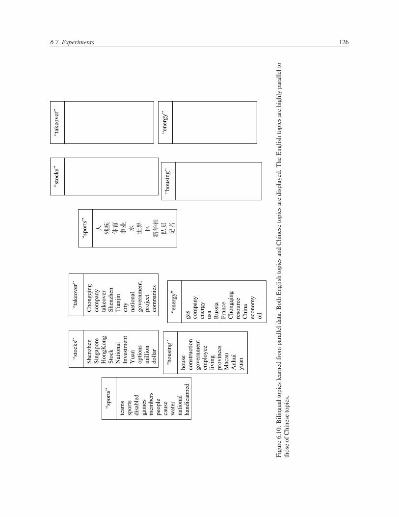
6.7. Experiments 126
“ho
usi
ng
”“e
ner
gy
”
“tak
eov
er”
“sto
cks”
“sp
ort
s”
team
s
spo
rts
dis
able
d
gam
es
mem
ber
s
peo
ple
cau
se
wat
er
nat
ion
al
han
dic
a pp
ed
Sh
enzh
en
Sin
gap
ore
HongK
ong
Sto
ck
Nat
ion
al
Inv
estm
ent
Yuan
op
tio
ns
mil
lio
n
do
lla r
Ch
on
gq
ing
com
pan
y
tak
eov
er
Sh
enzh
en
Tia
nji
n
city
nat
ion
al
go
ver
nm
ent,
pro
ject
com
pan
ies
ho
use
const
ruct
ion
go
ver
nm
ent
emp
loy
ee
liv
ing
pro
vin
ces
Mac
au
An
hu
i
yu
an
gas
com
pan
y
ener
gy
usa
Ru
ssia
Fra
nce
Ch
on
gq
ing
reso
urc
e
Ch
ina
eco
no
my
oil
“sp
ort
s”
“sto
cks”
“tak
eov
er”
“ho
usi
ng
”“e
ner
gy
”
Figu
re6.
10:B
iling
ualt
opic
sle
arne
dfr
ompa
ralle
ldat
a.B
oth
Eng
lish
topi
csan
dC
hine
seto
pics
are
disp
laye
d.T
heE
nglis
hto
pics
are
high
lypa
ralle
lto
thos
eof
Chi
nese
topi
cs.
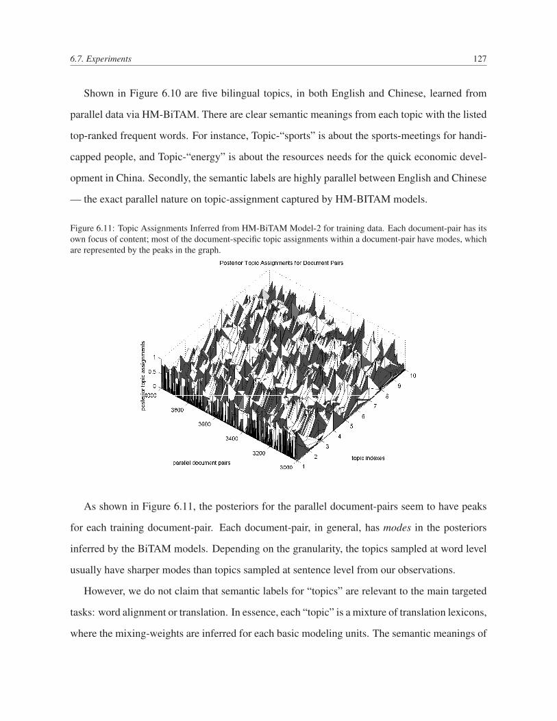
6.7. Experiments 127
Shown in Figure 6.10 are five bilingual topics, in both English and Chinese, learned from
parallel data via HM-BiTAM. There are clear semantic meanings from each topic with the listed
top-ranked frequent words. For instance, Topic-“sports” is about the sports-meetings for handi-
capped people, and Topic-“energy” is about the resources needs for the quick economic devel-
opment in China. Secondly, the semantic labels are highly parallel between English and Chinese
— the exact parallel nature on topic-assignment captured by HM-BITAM models.
Figure 6.11: Topic Assignments Inferred from HM-BiTAM Model-2 for training data. Each document-pair has itsown focus of content; most of the document-specific topic assignments within a document-pair have modes, whichare represented by the peaks in the graph.
As shown in Figure 6.11, the posteriors for the parallel document-pairs seem to have peaks
for each training document-pair. Each document-pair, in general, has modes in the posteriors
inferred by the BiTAM models. Depending on the granularity, the topics sampled at word level
usually have sharper modes than topics sampled at sentence level from our observations.
However, we do not claim that semantic labels for “topics” are relevant to the main targeted
tasks: word alignment or translation. In essence, each “topic” is a mixture of translation lexicons,
where the mixing-weights are inferred for each basic modeling units. The semantic meanings of

6.7. Experiments 128
the topics are not what we are optimizing within the proposed BiTAM framework. The sharper
resolutions of topics might not necessarily correlate well with higher word-alignment accuracies
nor translation quality. Instead, the topics inferred give clues to the quality of BiTAM models,
but other measures such as training and test set likelihood and word-alignment accuracies are
more relevant to evaluate the proposed BiTAM models, and the comparing with IBM models is
more meaningful.
6.7.4 Improved Likelihood and Perplexity for BiTAMs
To answer the first question listed in section 6.7: can the proposed BiTAM models improve the
modeling power, the perplexities for both training data and test data were computed. Perplexities
were also divided into word-length specific components as shown in Table 6.6.
Perplexity is usually a good metric for measuring the modeling power using esp. unseen data.
For translation models, we can usually decompose the perplexity into two major components:
one from position choice within a sentence-pair, and one from lexical choice for selecting a
word’s translation. For Chinese-English, the perplexity is also highly dependent on the nature of
the Chinese word-segmenter applied. In all the experiments, Stanford word-segmenter (Tseng
et al., 2005), which was learned following the Chinese treebank style, was applied to the data.
In Table 6.6, the components configuration of perplexity are listed for IBM Models, and
BiTAM models. The position component usually helps to narrow down the choices for word-
alignment. Therefore, as shown in the experiments, those models with position-component, such
as HMM, IBM Model-4, and HM-BiTAM, usually have lower perplexity than those without.
Models IBM-1 HMM IBM-4 BiTAM-1 BiTAM-2 BiTAM-3 HM-BiTAM-1 HM-BiTAM-2Position No Yes Yes No No No Yes YesLexicon Yes Yes Yes Yes Yes Yes Yes Yes
Table 6.6: The perplexity components for IBM Models, HMM and BiTAMs.
BiTAM Model-1 has embedded IBM Model-1 alignment; the perplexity and likelihood of the
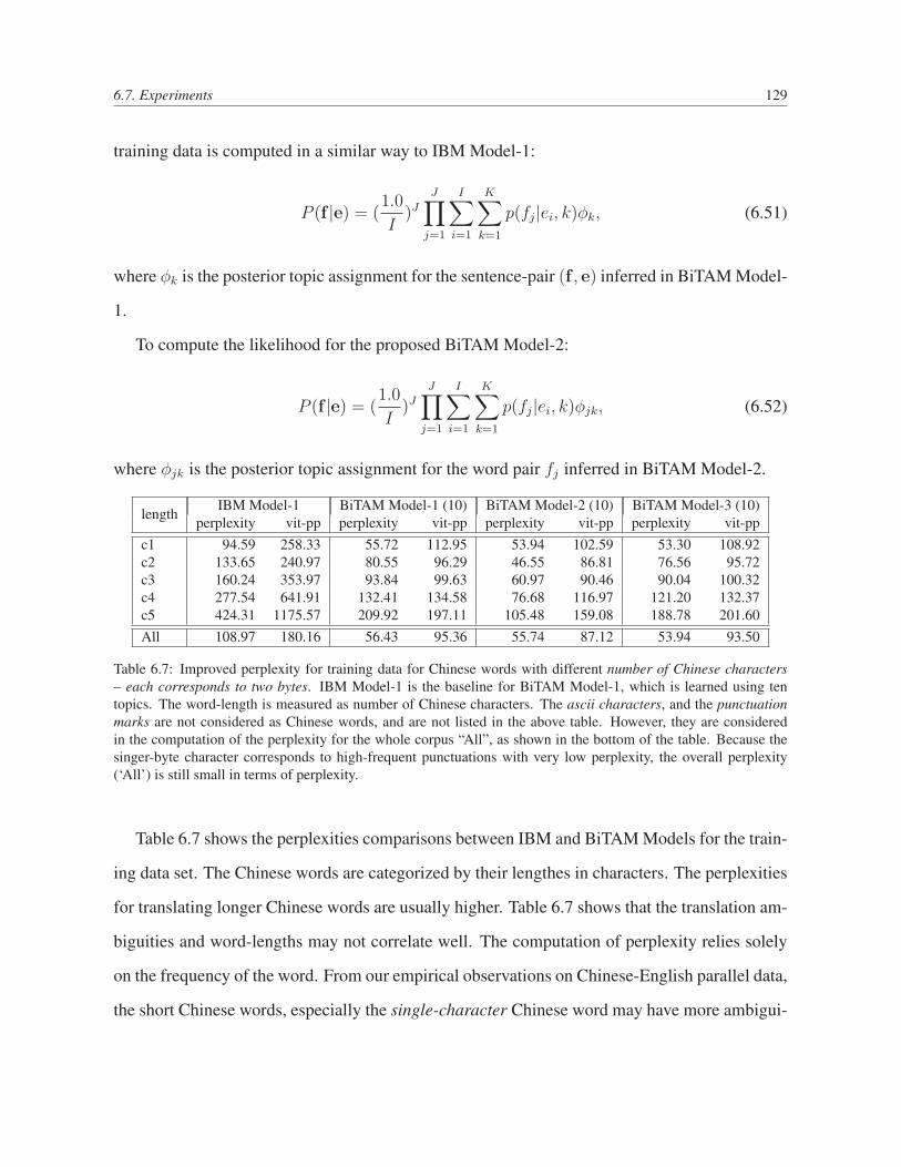
6.7. Experiments 129
training data is computed in a similar way to IBM Model-1:
P (f |e) = (1.0
I)J
J∏j=1
I∑i=1
K∑
k=1
p(fj|ei, k)φk, (6.51)
where φk is the posterior topic assignment for the sentence-pair (f , e) inferred in BiTAM Model-
1.
To compute the likelihood for the proposed BiTAM Model-2:
P (f |e) = (1.0
I)J
J∏j=1
I∑i=1
K∑
k=1
p(fj|ei, k)φjk, (6.52)
where φjk is the posterior topic assignment for the word pair fj inferred in BiTAM Model-2.
length IBM Model-1 BiTAM Model-1 (10) BiTAM Model-2 (10) BiTAM Model-3 (10)perplexity vit-pp perplexity vit-pp perplexity vit-pp perplexity vit-pp
c1 94.59 258.33 55.72 112.95 53.94 102.59 53.30 108.92c2 133.65 240.97 80.55 96.29 46.55 86.81 76.56 95.72c3 160.24 353.97 93.84 99.63 60.97 90.46 90.04 100.32c4 277.54 641.91 132.41 134.58 76.68 116.97 121.20 132.37c5 424.31 1175.57 209.92 197.11 105.48 159.08 188.78 201.60All 108.97 180.16 56.43 95.36 55.74 87.12 53.94 93.50
Table 6.7: Improved perplexity for training data for Chinese words with different number of Chinese characters– each corresponds to two bytes. IBM Model-1 is the baseline for BiTAM Model-1, which is learned using tentopics. The word-length is measured as number of Chinese characters. The ascii characters, and the punctuationmarks are not considered as Chinese words, and are not listed in the above table. However, they are consideredin the computation of the perplexity for the whole corpus “All”, as shown in the bottom of the table. Because thesinger-byte character corresponds to high-frequent punctuations with very low perplexity, the overall perplexity(‘All’) is still small in terms of perplexity.
Table 6.7 shows the perplexities comparisons between IBM and BiTAM Models for the train-
ing data set. The Chinese words are categorized by their lengthes in characters. The perplexities
for translating longer Chinese words are usually higher. Table 6.7 shows that the translation am-
biguities and word-lengths may not correlate well. The computation of perplexity relies solely
on the frequency of the word. From our empirical observations on Chinese-English parallel data,
the short Chinese words, especially the single-character Chinese word may have more ambigui-
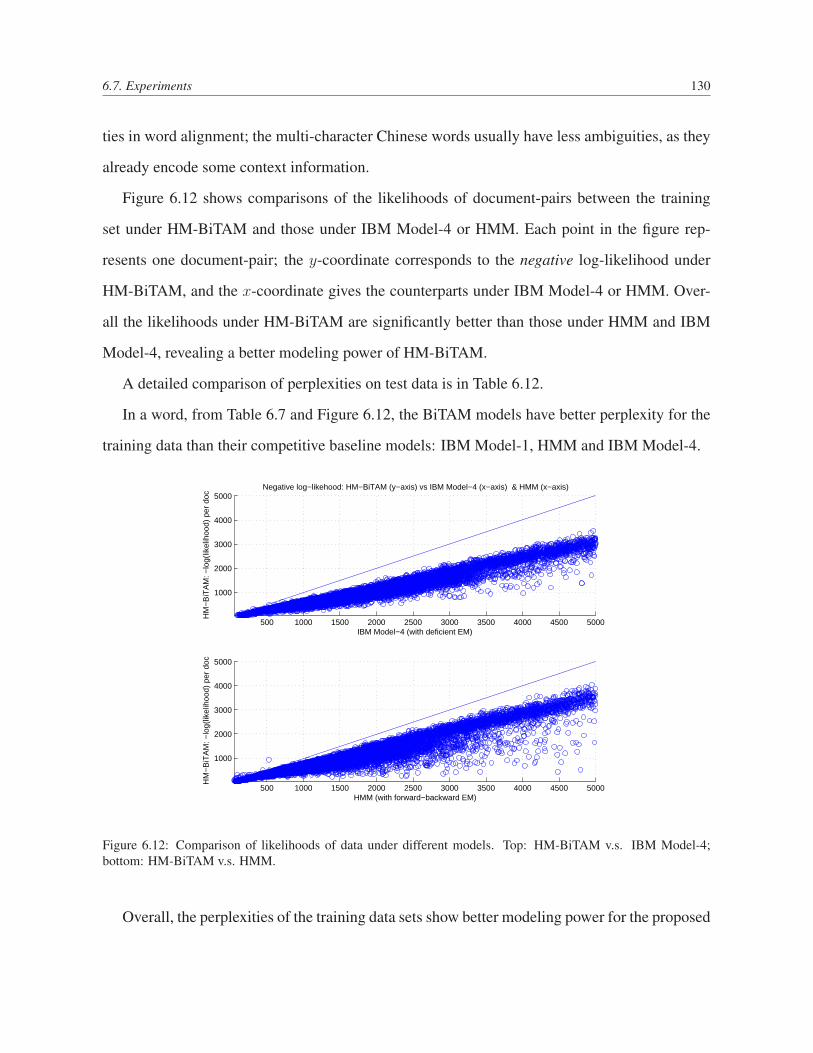
6.7. Experiments 130
ties in word alignment; the multi-character Chinese words usually have less ambiguities, as they
already encode some context information.
Figure 6.12 shows comparisons of the likelihoods of document-pairs between the training
set under HM-BiTAM and those under IBM Model-4 or HMM. Each point in the figure rep-
resents one document-pair; the y-coordinate corresponds to the negative log-likelihood under
HM-BiTAM, and the x-coordinate gives the counterparts under IBM Model-4 or HMM. Over-
all the likelihoods under HM-BiTAM are significantly better than those under HMM and IBM
Model-4, revealing a better modeling power of HM-BiTAM.
A detailed comparison of perplexities on test data is in Table 6.12.
In a word, from Table 6.7 and Figure 6.12, the BiTAM models have better perplexity for the
training data than their competitive baseline models: IBM Model-1, HMM and IBM Model-4.
500 1000 1500 2000 2500 3000 3500 4000 4500 5000
1000
2000
3000
4000
5000Negative log−likehood: HM−BiTAM (y−axis) vs IBM Model−4 (x−axis) & HMM (x−axis)
IBM Model−4 (with deficient EM)
HM
−B
iTA
M: −
log(
likel
ihoo
d) p
er d
oc
500 1000 1500 2000 2500 3000 3500 4000 4500 5000
1000
2000
3000
4000
5000
HM
−B
iTA
M: −
log(
likel
ihoo
d) p
er d
oc
HMM (with forward−backward EM)
Figure 6.12: Comparison of likelihoods of data under different models. Top: HM-BiTAM v.s. IBM Model-4;bottom: HM-BiTAM v.s. HMM.
Overall, the perplexities of the training data sets show better modeling power for the proposed
6.7. Experiments 131
BiTAM models than their competing IBM models. Similar experiments were carried out for
unseen test sets, as will shown in Table 6.12. Since the topic-specific lexicon is the major factor
different from IBM models, we further investigate these translation lexicons by looking into
three specific measures. First, each English word invokes a simplex, and the entropy can be
defined for each English word as in Eqn. 6.53. The entropy reflects how confident the lexicon
p(f |e, k) is on the translations of a given English word e.
H(f |e) = −∑
f∈VF
p(f |e) · log p(f |e). (6.53)
The second measure proposed is the L2-norm. This measure is to describe the shape of the
lexicon’s distribution. It emphasizes the probability mass allocated for the top-ranked translation
candidates for a given English word e. If the top-ranked candidates occupy large probability
mass, the L2-norm will also be large. A large L2-norm value indicates that the distribution
peaks around the top-ranked candidates, and the lexicon is considered to be sharp. To compute
the L2 Norm, we have:
S(f |e) =∑
f∈VF
p(f |e)2. (6.54)
The third measure we take is the “epsilon-95%”, which is an empirical measure of the “fuzzi-
ness” of a lexicon. For a given English word, we count how many of the proposed translation
candidates pass the threshold of p(f |e, k) > 0.05. This a very rough measure to tell how skewed
the lexicon’s distribution is. We also look into the number of the unique word-pairs in the trans-
lation lexicon table.
Table 6.8 shows the average entropy, L2-Norm, epsilon-95% and lexicon’s size for baseline
IBM Models and HMM, and BiTAM Models. The IBM Model-1 lexicon has an averaged en-
tropy of 2.20, while the lowest entropy from the proposed BiTAM topic-specific lexicons is 1.73
for BiTAM Model-1 and 1.41 for BiTAM Model-2. The measurements of L2-norm and epsilon-
95% also show similar trends. These evidences indicate the lexicons inferred from BiTAM
6.7. Experiments 132
models are sharper than the baseline IBM Model-1 lexicons. Each individual topic-specific lex-
icon is smaller in sizes than IBM model-1, and in general, the BiTAM models do not introduce
too many additional parameters over IBM models. Note, these measures are only used as side
evidences for the lexicons which are learned from well defined models; the proposed models are
not designed to optimize towards these measures.
Another observation from Table 6.8 is: BiTAM Model-3 and HM-BiTAM Model-2 have more
evenly spread entropy and L2-Norm than other models. Presumably, BiTAM Model-3 introduces
monolingual topic-specific unigram to enhance the prior, which helps smoothing across the top-
ics. HM-BiTAM Model-2 sample a topic for each word-pair instead of for each sentence-pair. In
this way, more samples of topic evidences (for example 400 instead of 20 at sentence-pair level)
are collected for updating the topic-assignment prior; this seems to reduce the variance across
different topics. BiTAM Model-2, which samples topics for each word-pair, obviously has more
evenly distributed lexicons than BiTAM Model-1, esp. in terms of the lexicon’s sizes. The same
picture is exemplified for HM-BiTAM Model-2 versus HM-BiTAM Model-1.
6.7.5 Evaluating Word Alignment
Word alignment accuracies were evaluated in a few settings. Notably, the proposed BiTAM
models are generative models in the spirit of the noisy channel model, similar to the IBM models.
Therefore, BiTAM models allow to leverage alignments in both directions: English-to-Chinese
(EC) and Chinese-to-English (CE).
Similar heuristics applied to state-of-the-art SMT systems can also be applied to BiTAM
alignments and phrase-extractions. For instance, the heuristics from Koehn (2004a) can be ap-
plied on the word alignment matrix to tune the system for better alignment or translation quali-
ties. INTER takes the intersection of the two directions and generates high-precision and high-
confident alignments; the UNION of two directions gives high-recall with additional aligned
points; REFINED grows the intersection with the neighboring word-pairs seen in the union, and
yields high-precision and high-recall alignments.
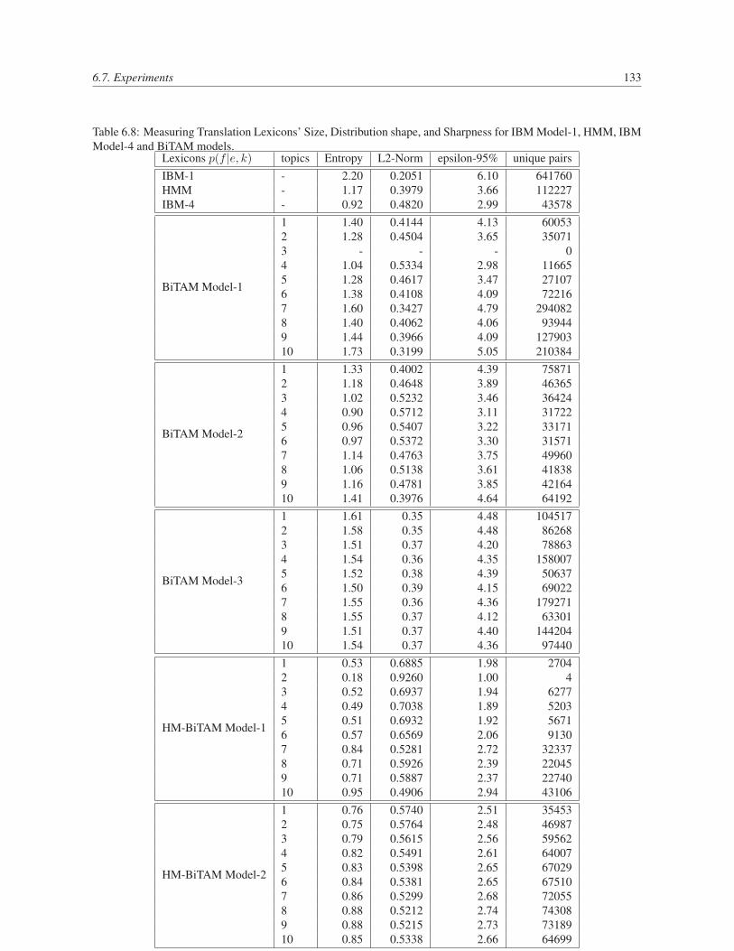
6.7. Experiments 133
Table 6.8: Measuring Translation Lexicons’ Size, Distribution shape, and Sharpness for IBM Model-1, HMM, IBMModel-4 and BiTAM models.
Lexicons p(f |e, k) topics Entropy L2-Norm epsilon-95% unique pairsIBM-1 - 2.20 0.2051 6.10 641760HMM - 1.17 0.3979 3.66 112227IBM-4 - 0.92 0.4820 2.99 43578
BiTAM Model-1
1 1.40 0.4144 4.13 600532 1.28 0.4504 3.65 350713 - - - 04 1.04 0.5334 2.98 116655 1.28 0.4617 3.47 271076 1.38 0.4108 4.09 722167 1.60 0.3427 4.79 2940828 1.40 0.4062 4.06 939449 1.44 0.3966 4.09 12790310 1.73 0.3199 5.05 210384
BiTAM Model-2
1 1.33 0.4002 4.39 758712 1.18 0.4648 3.89 463653 1.02 0.5232 3.46 364244 0.90 0.5712 3.11 317225 0.96 0.5407 3.22 331716 0.97 0.5372 3.30 315717 1.14 0.4763 3.75 499608 1.06 0.5138 3.61 418389 1.16 0.4781 3.85 4216410 1.41 0.3976 4.64 64192
BiTAM Model-3
1 1.61 0.35 4.48 1045172 1.58 0.35 4.48 862683 1.51 0.37 4.20 788634 1.54 0.36 4.35 1580075 1.52 0.38 4.39 506376 1.50 0.39 4.15 690227 1.55 0.36 4.36 1792718 1.55 0.37 4.12 633019 1.51 0.37 4.40 14420410 1.54 0.37 4.36 97440
HM-BiTAM Model-1
1 0.53 0.6885 1.98 27042 0.18 0.9260 1.00 43 0.52 0.6937 1.94 62774 0.49 0.7038 1.89 52035 0.51 0.6932 1.92 56716 0.57 0.6569 2.06 91307 0.84 0.5281 2.72 323378 0.71 0.5926 2.39 220459 0.71 0.5887 2.37 2274010 0.95 0.4906 2.94 43106
HM-BiTAM Model-2
1 0.76 0.5740 2.51 354532 0.75 0.5764 2.48 469873 0.79 0.5615 2.56 595624 0.82 0.5491 2.61 640075 0.83 0.5398 2.65 670296 0.84 0.5381 2.65 675107 0.86 0.5299 2.68 720558 0.88 0.5212 2.74 743089 0.88 0.5215 2.73 7318910 0.85 0.5338 2.66 64699
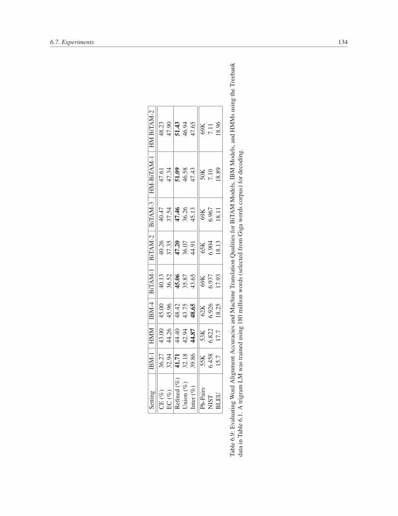
6.7. Experiments 134
Setti
ngIB
M-1
HM
MIB
M-4
BiT
AM
-1B
iTA
M-2
BiT
AM
-3H
M-B
iTA
M-1
HM
BiT
AM
-2
CE
(%)
36.2
743
.00
45.0
040
.13
40.2
640
.47
47.6
148
.23
EC
(%)
32.9
444
.26
45.9
636
.52
37.3
537
.54
47.3
447
.90
Refi
ned
(%)
41.7
144
.40
48.4
245
.06
47.2
047
.46
51.0
951
.43
Uni
on(%
)32
.18
42.9
443
.75
35.8
736
.07
36.2
646
.58
46.9
4In
ter(
%)
39.8
644
.87
48.6
543
.65
44.9
145
.13
47.4
347
.65
Ph-P
airs
55K
53K
62K
69K
65K
69K
50K
69K
NIS
T6.
458
6.82
26.
926
6.93
76.
904
6.96
77.
107.
11B
LE
U15
.717
.718
.25
17.9
318
.13
18.1
118
.89
18.9
6
Tabl
e6.
9:E
valu
atin
gW
ord
Alig
nmen
tAcc
urac
ies
and
Mac
hine
Tran
slat
ion
Qua
litie
sfo
rBiT
AM
Mod
els,
IBM
Mod
els,
and
HM
Ms
usin
gth
eTr
eeba
nkda
tain
Tabl
e6.
1.A
trig
ram
LM
was
trai
ned
usin
g18
0m
illio
nw
ords
(sel
ecte
dfr
omG
iga
wor
dsco
rpus
)for
deco
ding
.
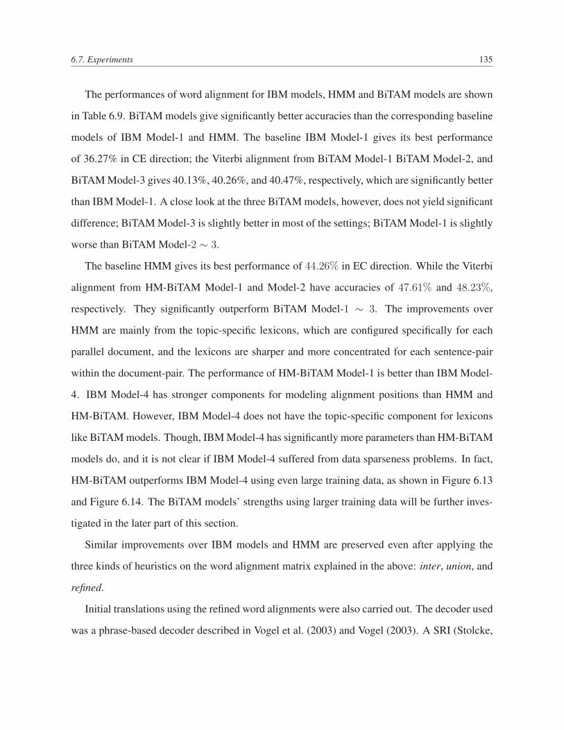
6.7. Experiments 135
The performances of word alignment for IBM models, HMM and BiTAM models are shown
in Table 6.9. BiTAM models give significantly better accuracies than the corresponding baseline
models of IBM Model-1 and HMM. The baseline IBM Model-1 gives its best performance
of 36.27% in CE direction; the Viterbi alignment from BiTAM Model-1 BiTAM Model-2, and
BiTAM Model-3 gives 40.13%, 40.26%, and 40.47%, respectively, which are significantly better
than IBM Model-1. A close look at the three BiTAM models, however, does not yield significant
difference; BiTAM Model-3 is slightly better in most of the settings; BiTAM Model-1 is slightly
worse than BiTAM Model-2 ∼ 3.
The baseline HMM gives its best performance of 44.26% in EC direction. While the Viterbi
alignment from HM-BiTAM Model-1 and Model-2 have accuracies of 47.61% and 48.23%,
respectively. They significantly outperform BiTAM Model-1 ∼ 3. The improvements over
HMM are mainly from the topic-specific lexicons, which are configured specifically for each
parallel document, and the lexicons are sharper and more concentrated for each sentence-pair
within the document-pair. The performance of HM-BiTAM Model-1 is better than IBM Model-
4. IBM Model-4 has stronger components for modeling alignment positions than HMM and
HM-BiTAM. However, IBM Model-4 does not have the topic-specific component for lexicons
like BiTAM models. Though, IBM Model-4 has significantly more parameters than HM-BiTAM
models do, and it is not clear if IBM Model-4 suffered from data sparseness problems. In fact,
HM-BiTAM outperforms IBM Model-4 using even large training data, as shown in Figure 6.13
and Figure 6.14. The BiTAM models’ strengths using larger training data will be further inves-
tigated in the later part of this section.
Similar improvements over IBM models and HMM are preserved even after applying the
three kinds of heuristics on the word alignment matrix explained in the above: inter, union, and
refined.
Initial translations using the refined word alignments were also carried out. The decoder used
was a phrase-based decoder described in Vogel et al. (2003) and Vogel (2003). A SRI (Stolcke,
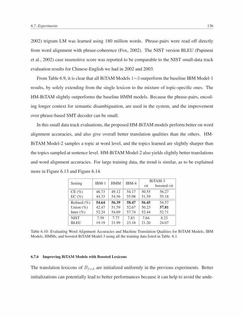
6.7. Experiments 136
2002) trigram LM was learned using 180 million words. Phrase-pairs were read off directly
from word alignment with phrase-coherence (Fox, 2002). The NIST version BLEU (Papineni
et al., 2002) case insensitive score was reported to be comparable to the NIST small-data track
evaluation results for Chinese-English we had in 2002 and 2003.
From Table 6.9, it is clear that all BiTAM Models 1∼3 outperform the baseline IBM Model-1
results, by solely extending from the single lexicon to the mixture of topic-specific ones. The
HM-BiTAM slightly outperforms the baseline HMM models. Because the phrase-pairs, encod-
ing longer context for semantic disambiguation, are used in the system, and the improvement
over phrase-based SMT decoder can be small.
In this small data track evaluations, the proposed HM-BiTAM models perform better on word
alignment accuracies, and also give overall better translation qualities than the others. HM-
BiTAM Model-2 samples a topic at word level, and the topics learned are slightly sharper than
the topics sampled at sentence level. HM-BiTAM Model-2 also yields slightly better translations
and word alignment accuracies. For large training data, the trend is similar, as to be explained
more in Figure 6.13 and Figure 6.14.
Setting IBM-1 HMM IBM-4 BiTAM-3vit boosted-vit
CE (%) 46.73 49.12 54.17 50.55 56.27EC (%) 44.33 54.56 55.08 51.59 55.18
Refined (%) 54.64 56.39 58.47 56.45 54.57Union (%) 42.47 51.59 52.67 50.23 57.81Inter (%) 52.24 54.69 57.74 52.44 52.71NIST 7.59 7.77 7.83 7.64 8.23BLEU 19.19 21.99 23.18 21.20 24.07
Table 6.10: Evaluating Word Alignment Accuracies and Machine Translation Qualities for BiTAM Models, IBMModels, HMMs, and boosted BiTAM Model-3 using all the training data listed in Table. 6.1.
6.7.6 Improving BiTAM Models with Boosted Lexicons
The translation lexicons of Bf,e,k are initialized uniformly in the previous experiments. Better
initializations can potentially lead to better performances because it can help to avoid the unde-
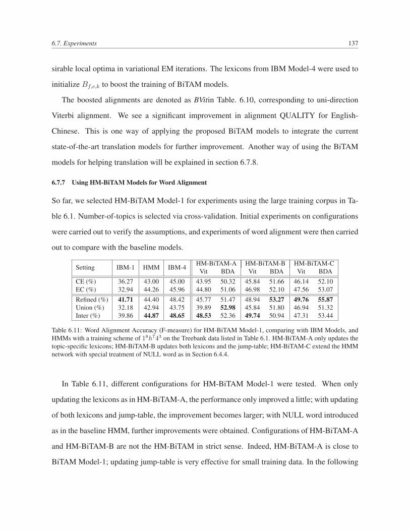
6.7. Experiments 137
sirable local optima in variational EM iterations. The lexicons from IBM Model-4 were used to
initialize Bf,e,k to boost the training of BiTAM models.
The boosted alignments are denoted as BVitin Table. 6.10, corresponding to uni-direction
Viterbi alignment. We see a significant improvement in alignment QUALITY for English-
Chinese. This is one way of applying the proposed BiTAM models to integrate the current
state-of-the-art translation models for further improvement. Another way of using the BiTAM
models for helping translation will be explained in section 6.7.8.
6.7.7 Using HM-BiTAM Models for Word Alignment
So far, we selected HM-BiTAM Model-1 for experiments using the large training corpus in Ta-
ble 6.1. Number-of-topics is selected via cross-validation. Initial experiments on configurations
were carried out to verify the assumptions, and experiments of word alignment were then carried
out to compare with the baseline models.
Setting IBM-1 HMM IBM-4 HM-BiTAM-A HM-BiTAM-B HM-BiTAM-CVit BDA Vit BDA Vit BDA
CE (%) 36.27 43.00 45.00 43.95 50.32 45.84 51.66 46.14 52.10EC (%) 32.94 44.26 45.96 44.80 51.06 46.98 52.10 47.56 53.07
Refined (%) 41.71 44.40 48.42 45.77 51.47 48.94 53.27 49.76 55.87Union (%) 32.18 42.94 43.75 39.89 52.98 45.84 51.80 46.94 51.32Inter (%) 39.86 44.87 48.65 48.53 52.36 49.74 50.94 47.31 53.44
Table 6.11: Word Alignment Accuracy (F-measure) for HM-BiTAM Model-1, comparing with IBM Models, andHMMs with a training scheme of 18h743 on the Treebank data listed in Table 6.1. HM-BiTAM-A only updates thetopic-specific lexicons; HM-BiTAM-B updates both lexicons and the jump-table; HM-BiTAM-C extend the HMMnetwork with special treatment of NULL word as in Section 6.4.4.
In Table 6.11, different configurations for HM-BiTAM Model-1 were tested. When only
updating the lexicons as in HM-BiTAM-A, the performance only improved a little; with updating
of both lexicons and jump-table, the improvement becomes larger; with NULL word introduced
as in the baseline HMM, further improvements were obtained. Configurations of HM-BiTAM-A
and HM-BiTAM-B are not the HM-BiTAM in strict sense. Indeed, HM-BiTAM-A is close to
BiTAM Model-1; updating jump-table is very effective for small training data. In the following

6.7. Experiments 138
experiments, we scaled up the training data size with the configuration to update both lexicons
and jump-table.
50
52
54
56
58
60
62
64
66
6M 11M 22.6M
HMM
BiTAM
IBM-4
HM-BiTAM
Figure 6.13: Experiments carried out using parallel corpora with up to 22.6-million (22.6 M) Chinese words. theword alignment accuracy (F-measure) over different sizes of training data, comparing with baseline HMMs.
Figure 6.14: Experiments carried out using parallel corpora with up to 22.6-million (23 M) Chinese words. Case-insensitive BLEU over MT03 (MER tuned on MT02) in a monotone SMT decoder.
Figure 6.13 shows the alignment accuracies of HM-BiTAM Models, in comparison with
those of the baseline-HMM, the baseline BiTAM Model-3, and the IBM Model-4. Overall,
HM-BiTAM gives significantly better F-measures over HMM, with absolute margins of 7.56%,
5.72% and 6.91% on training sizes of 6 M, 11 M and 22.6 M words, respectively. In HM-BiTAM,
two factors contribute to narrow down the word-alignment decisions: the position and the lexical
mapping. The position part is the same as the baseline-HMM, implementing the “proximity-

6.7. Experiments 139
bias”. Whereas the emission lexical probability is different, each state is a mixture of topic-
specific translation lexicons, of which the weights are inferred using document contexts. The
topic-specific translation lexicons are sharper and smaller than the global ones used in HMM.
Thus the improvements of HM-BiTAM over HMM are essentially resulted from the extended
topic-admixture lexicons. Not surprisingly, HM-BiTAM also outperforms the baseline-BiTAM
significantly, because BiTAM captures only the topical aspects but ignores the proximity bias.
Notably, HM-BiTAM also outperforms IBM Model-4 by a margin of 3.43%, 3.64% and
2.73%, respectively. IBM Model-4 already integrates the fertility and distortion sub-models on
top of HMM, which further narrow down the word-alignment choices. However, IBM Model-4
does not have a scheme to adjust its lexicon probabilities specific to document topical-context
as in HM-BiTAM. HM-BiTAM wins over IBM-4 by leveraging topic models that capture the
document context.
6.7.8 Decoding MT04 Documents in Gale07 System
We choose the shadow-data used in the GALE evaluation for the translation experiments. This
shadow-data contains 10 documents selected from NIST SMT04 evaluation. The genre cov-
ered are news, speech and editorial. Table 6.12 displayed several genres. The editorial usually
contains more subtle topics, as the authors do not share fixed patterns in presenting their opin-
ions. The topics covered in that ten documents range from spaceships, HIV issues, stock market,
terrorists, economic policies inside and outside of united states, etc..
The source documents were paired with one reference (“cha”), from a four-reference set. In
this way, we can compute the likelihood by applying different BiTAM models. The conditional
likelihood P (F |E) computed from our BiTAM models are shown in Table 6.12. HM-BiTAM
Model-2 yields the best conditional likelihood than other models. BiTAM Model-1∼3 are based
on embedded IBM Model-1 alignment model, and they have similar likelihoods for the ten
documents. We choose HM-BiTAM Model-2 for topic inference and investigate the potentials
for improving translations with the inferred topic assignments.
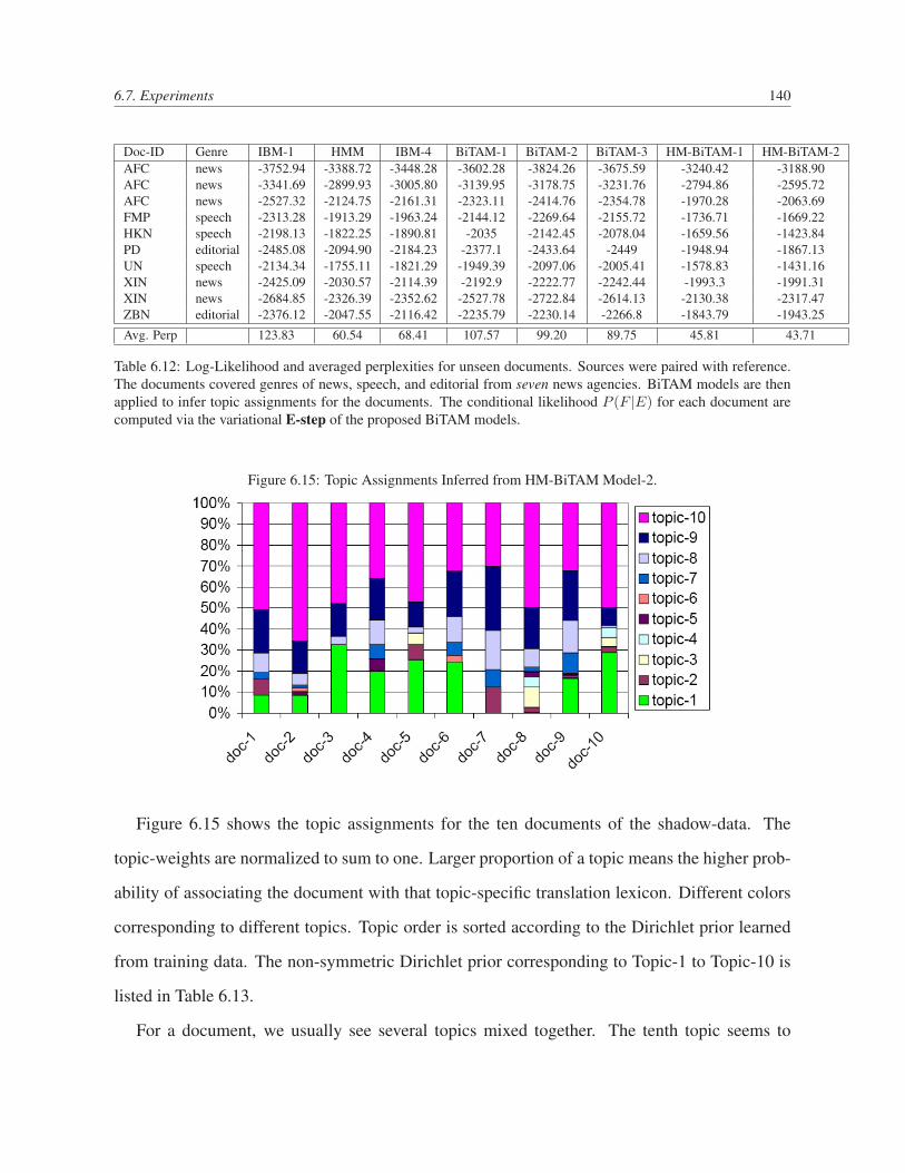
6.7. Experiments 140
Doc-ID Genre IBM-1 HMM IBM-4 BiTAM-1 BiTAM-2 BiTAM-3 HM-BiTAM-1 HM-BiTAM-2AFC news -3752.94 -3388.72 -3448.28 -3602.28 -3824.26 -3675.59 -3240.42 -3188.90AFC news -3341.69 -2899.93 -3005.80 -3139.95 -3178.75 -3231.76 -2794.86 -2595.72AFC news -2527.32 -2124.75 -2161.31 -2323.11 -2414.76 -2354.78 -1970.28 -2063.69FMP speech -2313.28 -1913.29 -1963.24 -2144.12 -2269.64 -2155.72 -1736.71 -1669.22HKN speech -2198.13 -1822.25 -1890.81 -2035 -2142.45 -2078.04 -1659.56 -1423.84PD editorial -2485.08 -2094.90 -2184.23 -2377.1 -2433.64 -2449 -1948.94 -1867.13UN speech -2134.34 -1755.11 -1821.29 -1949.39 -2097.06 -2005.41 -1578.83 -1431.16XIN news -2425.09 -2030.57 -2114.39 -2192.9 -2222.77 -2242.44 -1993.3 -1991.31XIN news -2684.85 -2326.39 -2352.62 -2527.78 -2722.84 -2614.13 -2130.38 -2317.47ZBN editorial -2376.12 -2047.55 -2116.42 -2235.79 -2230.14 -2266.8 -1843.79 -1943.25
Avg. Perp 123.83 60.54 68.41 107.57 99.20 89.75 45.81 43.71
Table 6.12: Log-Likelihood and averaged perplexities for unseen documents. Sources were paired with reference.The documents covered genres of news, speech, and editorial from seven news agencies. BiTAM models are thenapplied to infer topic assignments for the documents. The conditional likelihood P (F |E) for each document arecomputed via the variational E-step of the proposed BiTAM models.
Figure 6.15: Topic Assignments Inferred from HM-BiTAM Model-2.
Figure 6.15 shows the topic assignments for the ten documents of the shadow-data. The
topic-weights are normalized to sum to one. Larger proportion of a topic means the higher prob-
ability of associating the document with that topic-specific translation lexicon. Different colors
corresponding to different topics. Topic order is sorted according to the Dirichlet prior learned
from training data. The non-symmetric Dirichlet prior corresponding to Topic-1 to Topic-10 is
listed in Table 6.13.
For a document, we usually see several topics mixed together. The tenth topic seems to
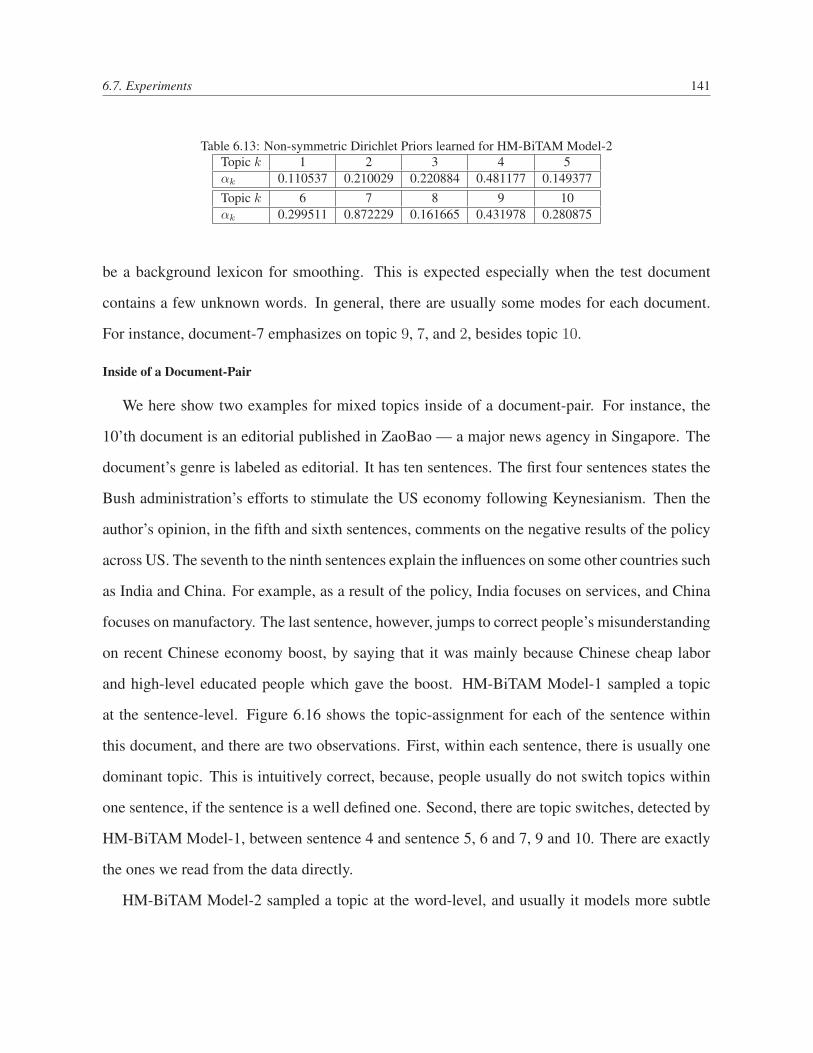
6.7. Experiments 141
Table 6.13: Non-symmetric Dirichlet Priors learned for HM-BiTAM Model-2Topic k 1 2 3 4 5αk 0.110537 0.210029 0.220884 0.481177 0.149377Topic k 6 7 8 9 10αk 0.299511 0.872229 0.161665 0.431978 0.280875
be a background lexicon for smoothing. This is expected especially when the test document
contains a few unknown words. In general, there are usually some modes for each document.
For instance, document-7 emphasizes on topic 9, 7, and 2, besides topic 10.
Inside of a Document-Pair
We here show two examples for mixed topics inside of a document-pair. For instance, the
10’th document is an editorial published in ZaoBao — a major news agency in Singapore. The
document’s genre is labeled as editorial. It has ten sentences. The first four sentences states the
Bush administration’s efforts to stimulate the US economy following Keynesianism. Then the
author’s opinion, in the fifth and sixth sentences, comments on the negative results of the policy
across US. The seventh to the ninth sentences explain the influences on some other countries such
as India and China. For example, as a result of the policy, India focuses on services, and China
focuses on manufactory. The last sentence, however, jumps to correct people’s misunderstanding
on recent Chinese economy boost, by saying that it was mainly because Chinese cheap labor
and high-level educated people which gave the boost. HM-BiTAM Model-1 sampled a topic
at the sentence-level. Figure 6.16 shows the topic-assignment for each of the sentence within
this document, and there are two observations. First, within each sentence, there is usually one
dominant topic. This is intuitively correct, because, people usually do not switch topics within
one sentence, if the sentence is a well defined one. Second, there are topic switches, detected by
HM-BiTAM Model-1, between sentence 4 and sentence 5, 6 and 7, 9 and 10. There are exactly
the ones we read from the data directly.
HM-BiTAM Model-2 sampled a topic at the word-level, and usually it models more subtle
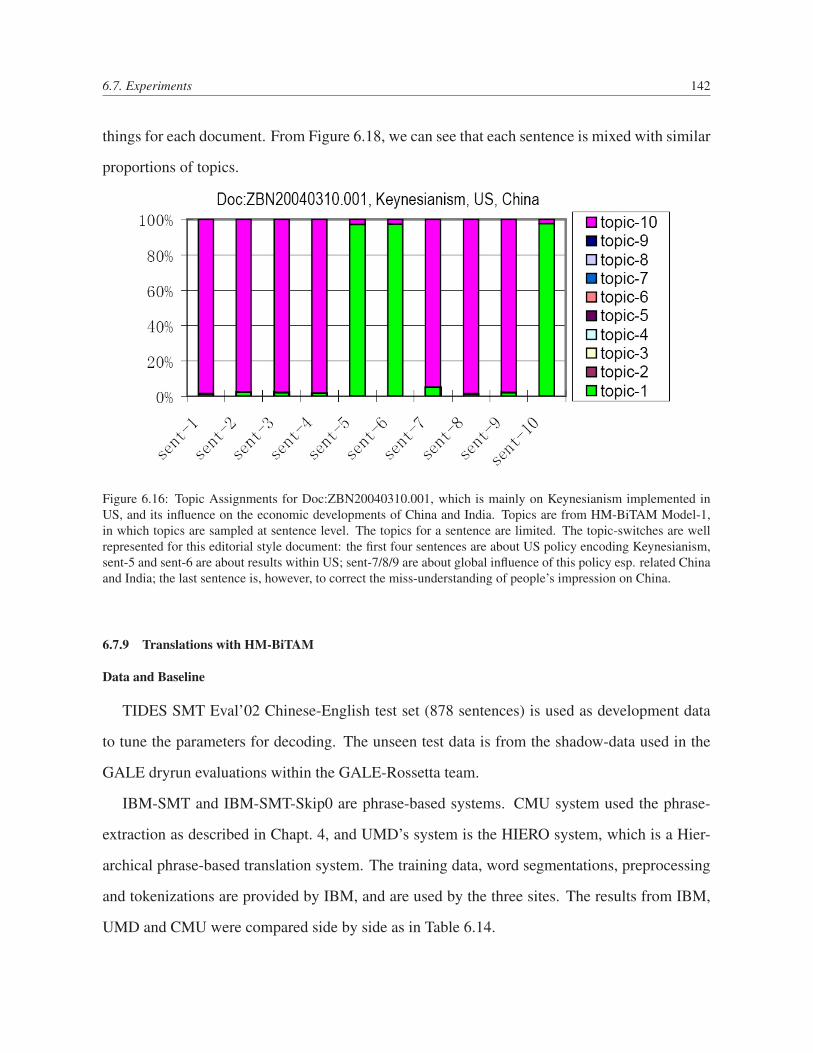
6.7. Experiments 142
things for each document. From Figure 6.18, we can see that each sentence is mixed with similar
proportions of topics.
Figure 6.16: Topic Assignments for Doc:ZBN20040310.001, which is mainly on Keynesianism implemented inUS, and its influence on the economic developments of China and India. Topics are from HM-BiTAM Model-1,in which topics are sampled at sentence level. The topics for a sentence are limited. The topic-switches are wellrepresented for this editorial style document: the first four sentences are about US policy encoding Keynesianism,sent-5 and sent-6 are about results within US; sent-7/8/9 are about global influence of this policy esp. related Chinaand India; the last sentence is, however, to correct the miss-understanding of people’s impression on China.
6.7.9 Translations with HM-BiTAM
Data and Baseline
TIDES SMT Eval’02 Chinese-English test set (878 sentences) is used as development data
to tune the parameters for decoding. The unseen test data is from the shadow-data used in the
GALE dryrun evaluations within the GALE-Rossetta team.
IBM-SMT and IBM-SMT-Skip0 are phrase-based systems. CMU system used the phrase-
extraction as described in Chapt. 4, and UMD’s system is the HIERO system, which is a Hier-
archical phrase-based translation system. The training data, word segmentations, preprocessing
and tokenizations are provided by IBM, and are used by the three sites. The results from IBM,
UMD and CMU were compared side by side as in Table 6.14.
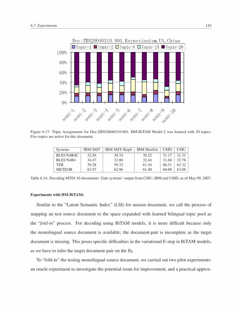
6.7. Experiments 143
Figure 6.17: Topic Assignments for Doc:ZBN20040310.001, HM-BiTAM Model-2 was learned with 20 topics.Five topics are active for this document.
Systems IBM-SMT IBM SMT-Skip0 IBM MaxEnt UMD CMUBLEUN4R4C 32.56 30.74 30.22 31.17 31.31BLEUN4R4 34.47 32.80 32.44 31.60 32.78TER 59.28 59.32 61.54 66.51 62.32METEOR 63.97 62.96 61.40 60.00 63.08
Table 6.14: Decoding MT04 10-documents: Gale systems’ output from CMU, IBM and UMD, as of May 09, 2007.
Experiments with HM-BiTAMs
Similar to the “Latent Semantic Index” (LSI) for unseen document, we call the process of
mapping an test source document to the space expanded with learned bilingual topic pool as
the “fold-in” process. For decoding using BiTAM models, it is more difficult because only
the monolingual source document is available; the document-pair is incomplete as the target
document is missing. This poses specific difficulties in the variational E-step in BiTAM models,
as we have to infer the target document-pair on the fly.
To “fold-in” the testing monolingual source document, we carried out two pilot experiments:
an oracle experiment to investigate the potential room for improvement, and a practical approx-
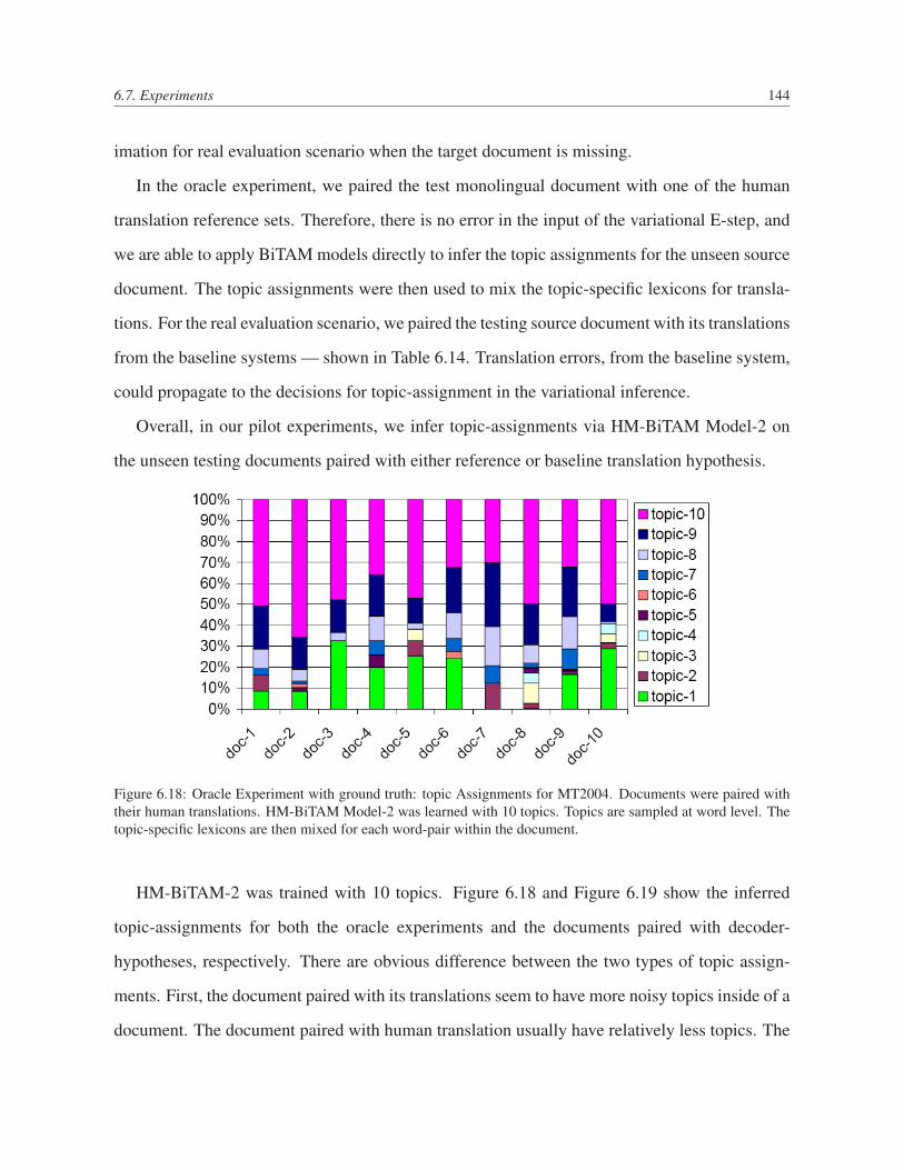
6.7. Experiments 144
imation for real evaluation scenario when the target document is missing.
In the oracle experiment, we paired the test monolingual document with one of the human
translation reference sets. Therefore, there is no error in the input of the variational E-step, and
we are able to apply BiTAM models directly to infer the topic assignments for the unseen source
document. The topic assignments were then used to mix the topic-specific lexicons for transla-
tions. For the real evaluation scenario, we paired the testing source document with its translations
from the baseline systems — shown in Table 6.14. Translation errors, from the baseline system,
could propagate to the decisions for topic-assignment in the variational inference.
Overall, in our pilot experiments, we infer topic-assignments via HM-BiTAM Model-2 on
the unseen testing documents paired with either reference or baseline translation hypothesis.
Figure 6.18: Oracle Experiment with ground truth: topic Assignments for MT2004. Documents were paired withtheir human translations. HM-BiTAM Model-2 was learned with 10 topics. Topics are sampled at word level. Thetopic-specific lexicons are then mixed for each word-pair within the document.
HM-BiTAM-2 was trained with 10 topics. Figure 6.18 and Figure 6.19 show the inferred
topic-assignments for both the oracle experiments and the documents paired with decoder-
hypotheses, respectively. There are obvious difference between the two types of topic assign-
ments. First, the document paired with its translations seem to have more noisy topics inside of a
document. The document paired with human translation usually have relatively less topics. The

6.7. Experiments 145
Figure 6.19: Practical Experiment: topic Assignments for MT2004., HM-BiTAM Model-2 was learned with 10topics. Testing document is paired with the top-1 baseline translation hypotheses. Topic assignment is inferred withHM-BiTAM Model-2; topic-specific lexicons are then mixed for each word-pair within the document.
first and the last topics (topic-1 and topic-10) seem to play larger role in the topic-assignment
from oracle experiments; while topic-6 seems to be everywhere when using the translation hy-
pothesis from the baseline system. The errors introduced from the baseline hypothesis are mostly
content words, which can influence the topic assignment significantly.
Given the inferred topic-assignment from either oracle document pair or practical hypoth-
esized document-pair, each sentence, in a document, is a mixture of topics; we can mix the
topic-specific lexicons using the inferred topic-weights as follows:
p(f |e,D) =K∑
k=1
p(f |e, k) · p(k|D), (6.55)
where D is a document; p(k|D) is the topic-weight assignment based on the document con-
text; p(f |e, k) is the topic-specific lexicons; p(f |e,D) is the mixed-lexicon from the AdMixture
Models. The mixed translation lexicon p(f |e,D) is used to re-score the phrase-pairs, and the
score will be specific to each sentence.
A third way is to exploit the parallelism of monolingual topics underlying in the parallel data.
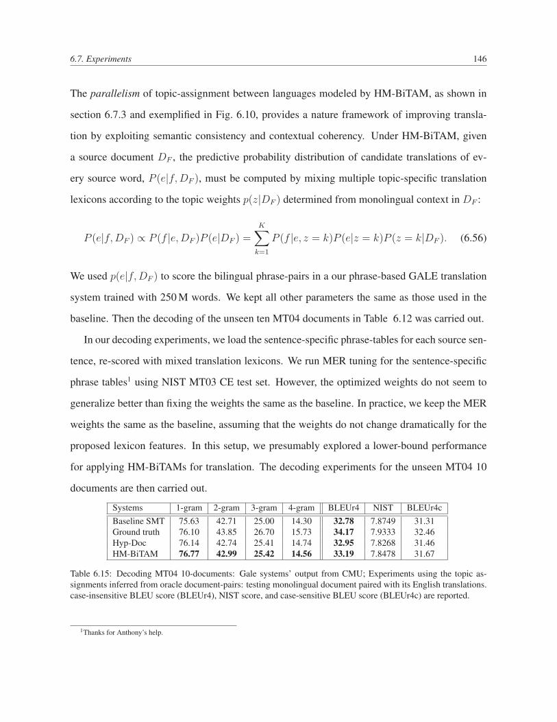
6.7. Experiments 146
The parallelism of topic-assignment between languages modeled by HM-BiTAM, as shown in
section 6.7.3 and exemplified in Fig. 6.10, provides a nature framework of improving transla-
tion by exploiting semantic consistency and contextual coherency. Under HM-BiTAM, given
a source document DF , the predictive probability distribution of candidate translations of ev-
ery source word, P (e|f, DF ), must be computed by mixing multiple topic-specific translation
lexicons according to the topic weights p(z|DF ) determined from monolingual context in DF :
P (e|f, DF ) ∝ P (f |e,DF )P (e|DF ) =K∑
k=1
P (f |e, z = k)P (e|z = k)P (z = k|DF ). (6.56)
We used p(e|f, DF ) to score the bilingual phrase-pairs in a our phrase-based GALE translation
system trained with 250 M words. We kept all other parameters the same as those used in the
baseline. Then the decoding of the unseen ten MT04 documents in Table 6.12 was carried out.
In our decoding experiments, we load the sentence-specific phrase-tables for each source sen-
tence, re-scored with mixed translation lexicons. We run MER tuning for the sentence-specific
phrase tables1 using NIST MT03 CE test set. However, the optimized weights do not seem to
generalize better than fixing the weights the same as the baseline. In practice, we keep the MER
weights the same as the baseline, assuming that the weights do not change dramatically for the
proposed lexicon features. In this setup, we presumably explored a lower-bound performance
for applying HM-BiTAMs for translation. The decoding experiments for the unseen MT04 10
documents are then carried out.
Systems 1-gram 2-gram 3-gram 4-gram BLEUr4 NIST BLEUr4cBaseline SMT 75.63 42.71 25.00 14.30 32.78 7.8749 31.31Ground truth 76.10 43.85 26.70 15.73 34.17 7.9333 32.46Hyp-Doc 76.14 42.74 25.41 14.74 32.95 7.8268 31.46HM-BiTAM 76.77 42.99 25.42 14.56 33.19 7.8478 31.67
Table 6.15: Decoding MT04 10-documents: Gale systems’ output from CMU; Experiments using the topic as-signments inferred from oracle document-pairs: testing monolingual document paired with its English translations.case-insensitive BLEU score (BLEUr4), NIST score, and case-sensitive BLEU score (BLEUr4c) are reported.
1Thanks for Anthony’s help.
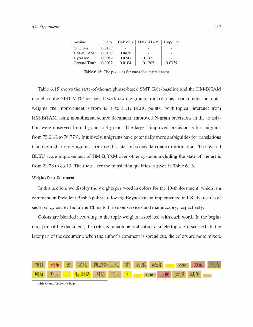
6.7. Experiments 147
p-value Hiero Gale-Sys HM-BiTAM Hyp-DocGale Sys 0.0127 - - -HM-BiTAM 0.0107 0.0430 - -Hyp-Doc 0.0052 0.0243 0.1921 -Ground Truth 0.0032 0.0104 0.1202 0.0339
Table 6.16: The p-values for one-tailed paired t-test
Table 6.15 shows the state-of-the-art phrase-based SMT Gale-baseline and the HM-BiTAM
model, on the NIST MT04 test set. If we know the ground truth of translation to infer the topic-
weights, the improvement is from 32.78 to 34.17 BLEU points. With topical inference from
HM-BiTAM using monolingual source document, improved N-gram precisions in the transla-
tion were observed from 1-gram to 4-gram. The largest improved precision is for unigram:
from 75.63% to 76.77%. Intuitively, unigrams have potentially more ambiguities for translations
than the higher order ngrams, because the later ones encode context information. The overall
BLEU score improvement of HM-BiTAM over other systems including the state-of-the-art is
from 32.78 to 33.19. The t-test 1 for the translation qualities is given in Table 6.16.
Weights for a Document
In this section, we display the weights per word in colors for the 10-th document, which is a
comment on President Bush’s policy following Keynesianism implemented in US; the results of
such policy enable India and China to thrive on services and manufactory, respectively.
Colors are blended according to the topic weights associated with each word. In the begin-
ning part of the document, the color is monotone, indicating a single topic is discussed. In the
later part of the document, when the author’s comment is spread out, the colors are more mixed.
布什 政府 想 采用 凯恩斯主义 来 刺激 经济 , one 方面 大力
增加 开支 ( 特别是 国防 开支 ) , one 方面 大量 减税 。
1with Kyung-Ah Sohn’s help.
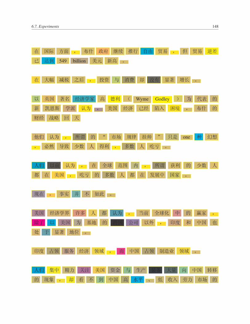
6.7. Experiments 148
在 国际 方面 , 布什 政府 继续 推行 自由 贸易 , 但 贸易 逆差
已 达到 549 billion 美元 新高 。
在 大幅 减税 之后 , 投资 与 消费 却 没有 显著 增长 。
以 英国 著名 经济学家 高 德利 ( Wyme Godley ) 为 代表 的
新 凯恩斯 学派 认为 , 美国 经济 已经 陷入 困境 , 布什 的
财经 战略 回 天
他们 认为 , 所谓 的 “ 市场 规律 挂帅 ” 只是 one 种 幻想
, 必然 导致 少数 人 得利 , 多数 人 吃亏 。
人们 以前 认为 , 在 全球 范围 内 , 所谓 获利 的 少数 人
都 在 美国 , 吃亏 的 多数 人 都 在 发展中 国家 。
现在 , 事实 并 不 如此 。
美国 经济学界 许多 人 都 认为 , 当前 全球化 中 的 赢家 ,
除了 以 美国 为 基地 的 跨国 公司 以外 , 印度 和 中国 也
处 于 显著 地位 。
印度 占领 服务 经济 领域 , 而 中国 占领 制造业 领域 。
人们 集中 精力 关注 美国 资金 与 生产 装备 大量 向 中国 转移
的 现象 , 却 看 不 到 中国 高 水平 、 低 收入 劳力 市场 的

6.8. Discussion and Summary 149
优势 。
6.8 Discussion and Summary
In this chapter, a novel framework, BiTAM, is presented to explore bilingual topics, and general-
ize over traditional IBM Model-1 and HMM for improved word-alignment accuracies and trans-
lation quality. A variational inference and learning procedure was developed for efficient training
based on generalized mean field. We demonstrated significant improvement of word-alignment
accuracy over a number of existing systems, and the interesting capability of HM-BiTAM to
simultaneously extract coherent monolingual topics from both languages. We also report en-
couraging improvement of translation quality over current benchmarks. Although the margin is
modest, it is noteworthy that the current version of HM-BiTAM remains a purely autonomously
trained system. Future work also includes extensions with more structures for word-alignment
such as noun phrase chunking, and also investigations of principle ways for selecting number of
topics to configure BiTAM for given training data sets.

Chapter 7
Summary of this Thesis
This thesis proposes new models for approximating the translational equivalence at different
levels: documents, sentences, phrases, words and concepts. The goal of this thesis is to enable
efficient “learning to translate” by sharing evidences of translational equivalence ranging from
concepts to feedbacks.
In Nida (1964), the professional translators’ behaviors can be divided into three rounds, which
can be further divided into nine steps. The first round involves reading the entire document and
obtaining background information; The second round involves comparing existing translations
and generating initial sufficiently comprehensible translations; The third round involves revis-
ing the translations from aspects including styles and rhythms, reactions of receptors, and the
scrutiny of other competent translators. Overall, these steps take into consideration various levels
of translational equivalence ranging from direct observations of word-pairs to hidden bilingual
topics from the document level.
This thesis focuses on models at three levels: mining parallel documents and sentences; mod-
eling hidden blocks learned from parallel sentences, modeling hidden bilingual topics inferred
from parallel document-pairs.
150
7.1. Survey of State-of-the-art Approaches 151
7.1 Survey of State-of-the-art Approaches
In this thesis, a detailed survey of state-of-the-art machine translation approaches is given. The
shortcomings of these approaches are pointed out, and addressed in later chapters. These ob-
servations and insights gained from literatures are summarized as the starting point for the work
in this thesis. Datasets and related issues are also explained for the development of this thesis,
especially the experimental parts.
The works of symmetrizing noisy channel models, EBMT, RBMT, and syntax based ap-
proaches all show that multiple information streams can enrich the expressiveness of the models
and thus improve the performances significantly. This requires a flexible framework in feature
selections, representations and integrations in statistical translation models.
7.2 Modeling Alignments of Document Pairs and Sentence Pairs
Data sparseness has been a bottleneck to NLP applications, especially for data-driven statistical
machine translation. Through the document and sentence level alignment models, the web’s
fast-growing, comparable data can be collected and filtered to be high quality parallel data to
improve translation performance or to adapt the models to a different domain.
The task of mining comparable documents and parallel sentences are challenging, as most of
the comparable documents contain much noise such as insertions or deletions. In addition, as the
web is so large, we need efficient tools for extracting the sentence-pairs from comparable data.
Usually some multi-stage models are designed in a divide-and-conquer style as seen in the pio-
neer work of Resnik and Smith (2003). The very relevant work is the cross-lingual information
retrieval with suitable designed query models.
Sentence alignment is usually thought of as a solved problem for cleanly aligned document
pairs. However, detailed study over 10 years of Xinhua news data (1992∼2001) showed the
ideal 1:1 aligned sentence pairs only occupy 60% percent of the whole data. For a much higher
quality FBIS data (2003/2002), it shows 1:1 mapping only accounts for 70% of the whole data.
7.3. Modeling Hidden Blocks 152
These previous studies show that length and lexicon information are both helpful, in different
aspects, for sentence alignment, so incorporating multiple information streams can bring more
benefits, as shown in this thesis.
7.3 Modeling Hidden Blocks
Most of the current approaches are based on the word-level mixture models such as IBM Models
1 ∼ 5 and HMMs. Context information is encoded in the phrase level translation pairs, which
are currently simply by-products of the word alignment models. Directly modeling the phrase-
pair is problematic because of the inherited complex dependencies between blocks and the curse
of dimensionality.
A block in a sentence pair corresponds to a phrase-pair translation. Blocks are usually short
and accurate in terms of localizing the word alignment choices. As most of the blocks are
inferred from word alignment, it is optimal to integrate the two into one optimization framework.
This thesis will show two different settings within one inner-outer bracketing framework. A
block brackets the sentence pair into two non-overlapping regions: the inner part and the outer
part. Within each part, a simpler alignment model can be applied to infer the word alignment
more accurately. Moreover, in this bracketing style, the interactions between phrase-pairs are
simplified. The inner part of a block is usually more effective in predicting the word alignment
than the outer part because its size is smaller.
Within the inner and outer parts, word alignment models such as the word-mixture models
or models with higher dependencies can be applied to infer better word alignment. The joint
likelihood can then be optimized together with the inner-outer segmentation via EM. This thesis
demonstrates significant improvements in the inner-outer model framework.
7.4 Modeling Hidden Concepts
The ultimate goal of machine translation is to abstract the meaning of a text from its forms and
reproduce the meaning in forms of a different language. In this process, the form and the code
7.4. Modeling Hidden Concepts 153
are changed while the meaning and the concepts are preserved.
Most machine translation systems treat the parallel data as isolated sentence pairs, ignoring
the concepts which unify the sentences into the original meaningful documents. A sentence,
taken out of the context of the document, is generally not very meaningful and less informative
in conveying the concepts. In fact, the parallel sentences come mostly from documents which
have certain logical concept flow. For example, the data provided by LDC is usually in one of
these categories: the high quality FBIS data, Sinorama data, Xinhua News, European Parliament
Plenary Sessions (EPPS) and the data from United Nations Debates. This thesis re-explains the
parallel sentences within their concept level translations.
Human beings do not make a sentence without a purpose. Each word conveys specific mean-
ings upon certain topics. The translation equivalence at the concept-level is subtle as the concepts
are bilingual. These hidden concepts can be learnt from bilingual document-pairs. With suit-
able representations of the bilingual concept, as proposed in this thesis, the parallel sentences
are generated in a manner similar to playing two “madlibs” simultaneously: pick up the aligned
structures first for both of the languages according to the certain hidden parallel concept distri-
bution; then pick up the words from the common topic specific distribution. This process can be
governed by a Dirichlet prior.
In this thesis, several BiTAM models are proposed and tested within this framework; they
generalize over the traditional IBM Model-1 and HMM for word alignment. Tractable learning
and inference are designed, and experiments in this thesis show we have better modeling power
from BiTAM models, which leads to better word-alignment accuracy and improved translation
quality.
References 154
References
De Finetti B. 1974. Theory of Probability. Wiley, New York.
Alexandra Birch, Miles Osborne, and Philipp Koehn. 2007. Ccg supertags in factored statisticalmachine translation. In ACL Workshop on Statistical Machine Translation.
David Blei, Andrew NG, and Michael I. Jordon. 2003. Latent dirichlet allocation. In Journal ofMachine Learning Research, volume 3, pages 1107–1135.
Lai J. C. Brown, P. and R. Mercer. 1991. Aligning sentences in parallel corpora. In ACL-91.
Peter F. Brown, Stephen A. Della Pietra, Vincent. J. Della Pietra, and Robert L. Mercer. 1993.The mathematics of statistical machine translation: Parameter estimation. In ComputationalLinguistics, volume 19(2), pages 263–331.
M. Carl and A. Way. 2003. Recent advances in Example-based Machine Translation. In Dor-drechtL Kluwer Academic Publishers, Phuket, Thailand.
Eugene Charniak, Kevin Knight, and Kenji Yamada. 2003. Syntax-based language models forstatistical machine translation. In Proceedings of MT Summit IX 2003, New Orleans.
Stanley F. Chen. 1993. Aligning sentences in bilingual corpora using lexical information. InThe 31st Annual Meeting of the Assoc. for Computational Linguistics (ACL93), Columbus,Ohio, June, June.
Colin Cherry and Dekang Lin. 2003. A probability model to improve word alignment. InProceedings of the Annual Meeting of the Association for Computational Linguistics.
David Chiang. 2005. A hierarchical phrase-based model for statistical machine translation.In Proceedings of the 43rd Annual Meeting of the Association for Computational Linguis-tics (ACL’05), pages 263–270, Ann Arbor, Michigan, June. Association for ComputationalLinguistics.
K. W. Church. 1993. Char align: A program for aligning parallel texts at the character level. InACL-93.
Herve Dejean, Eric Gaussier, Cyril Goutte, and Kenji Yamada. 2003. Reducing parameter spacefor word alignment. In Rada Mihalcea and Ted Pedersen, editors, HLT-NAACL 2003 Work-shop: Building and Using Parallel Texts: Data Driven Machine Translation and Beyond,pages 23–26, Edmonton, Alberta, Canada, May 31. Association for Computational Linguis-tics.
Elena Erosheva, Steve Fienberg, and John Lafferty. 2004. Mixed membership models of scien-tific publications. In Proceedings of the National Academy of Sciences, volume 101 of Suppl.1, April 6.
Heidi J. Fox. 2002. Phrasal cohesion and statistical machine translation. In Proc. of the Confer-ence on Empirical Methods in Natural Language Processing, pages 304–311, Philadelphia,PA, July 6-7.

References 155
Alexander Fraser and Daniel Marcu. 2006. Semi-supervised training for statistical word align-ment. In the Conference of the Association for Computational Linguistics (ACL), July.
W. A. Gale and K. W. Church. 1991. A program for aligning sentences in bilingual corpora. InACL-91.
Michel Galley, Jonathan Graehl, Kevin Knight, Daniel Marcu, Steve DeNeefe, Wei Wang, andIgnacio Thayer. 2006. Scalable inference and training of context-rich syntactic translationmodels. In Proceedings of ACL-Coling, pages 961–968, Australia, July.
JianFeng Gao and Jianyun Nie. 2006. Statistical query translation models for cross-languageinformation retrieval. In ACM Transactions on Asian Information Processing (TAKIP).
Niyu Ge. 2004. A maximum posterior method for word alignment. In Presentation given atDARPA/TIDES MT workshop.
Daniel Gildea. 2003. Loosely tree-based alignment for machine translation. In Proceedingsof the 41th Annual Conference of the Association for Computational Linguistics (ACL-03),pages 80–87, Sapporo, Japan.
Daniel Gildea. 2004. Dependencies vs. constituents for tree-based alignment. In 2004 Confer-ence on Empirical Methods in Natural Language Processing (EMNLP), Barcelona.
Jonathan Graehl and Kevin Knight. 2004. Training tree transducers. In Proc. NAACL-HLT.
Masahiko Haruno and Takefumi Yamazaki. 1996. High-performance bilingual text alignmentusing statistical and dictionary information. In Annual Meeting of the Association for Com-putationaly Linguistics.
Sanjika Hewavitharana, Bing Zhao, Almut Silja Hildebrand, Matthias Eck, Chiori Hori, StephanVogel, and Alex Waibel. 2005. The cmu statistical machine translation system for iwslt2005.In The 2005 International Workshop on Spoken Language Translation.
Fei Huang and Kishore Papineni. 2007. Hierarchical system combination for machine trans-lation. In the Joint Conference on Empirical Methods in Natural Language Processing andComputational Natural Language Learning (EMNLP-CoNLL 2007).
John Hutchins. 2005. Towards a definition of example-based machine translation. In MTSummit X workshop on Example-Based Machine Translation, pages 63–70, Phuket, Thailand,September,16.
R. Hwa, P. Resnik, A. Weinberg, and O. Kolak. 2002. Evaluating translational correspondenceusing annotation projection. In Proc of ACL.
Abraham Ittycheriah and Salim Roukos. 2005. A maximum entropy word aligner for arabic-english machine translation. In Human Language Technology Conference and EmpiricalMethods in Natural Language Processing.
Abraham Ittycheriah and Salim Roukos. 2007. Direct translation model 2. In Human LanguageTechnologies (HLT).
References 156
Paul B. Kanto and Ellen Voorhees. 1996. Report on the trec-5 confusion track. In The Fifth TextRetrieval Conference.
R. Kneser and Hermann Ney. 1993. Improved clustering techniques for class-based statisticallanguage modelling. In European Conference on Speech Communication and Technology,pages 973–976.
Philipp Koehn and Hieu Hoang. 2007. Factored translation models. In Joint Conference onEmpirical Methods in Natural Language Processing and Computational Natural LanguageLearning (EMNLP-CoNLL).
Philipp Koehn. 2003. Noun phrase translation. In Ph.D. Thesis, University of Southern Califor-nia, ISI.
Philipp Koehn. 2004a. The foundation for statistical machine translation at mit. In Presentationgiven at DARPA/TIDES MT workshop.
Philipp Koehn. 2004b. Pharaoh: a beam search decoder for phrase-based smt. In Proceedingsof the Conference of the Association for Machine Translation in the Americans (AMTA).
Tz-Liang Kueng and Keh-Yih Su. 2002. A robust cross-style bilingual sentences alignmentmodel. In International Conference on Computational Linguistics (Coling).
S. Lacoste-Julien, B Taskar, D. Klein, and M. Jordan. 2006. Word alignment via quadraticassignment. In Human Language Technology conference.
Young-Suk Lee. 2004. Morphological analysis for statistical machine translation. In HumanLanguage Technologies Conference (HLT).
P. Liang, Alexandre Bouchard-Cote, Dan Klein, and Ben. Taskar. 2006a. An end-to-end dis-criminative approach to machine translation. In ACL.
P. Liang, B. Taskar, and D. Klei. 2006b. Alignment by agreement. In Human Language Tech-nology conference (HLT).
Yang Liu, Qun Liu, and Shouxun Lin. 2005. Log-linear models for word alignment. In Proceed-ings of the 43rd Annual Meeting of the Association for Computational Linguistics (ACL’05),pages 459–466, Ann Arbor, Michigan, June. Association for Computational Linguistics.
Xiaoyi Ma and Mark Y. Liberman. 1999. Bits: A method for bilingual text search over the web.In Machine Translation Summit VII.
Marina Meila and Jianbo Shi. 2000. Learning segmentation by random walks. In Advances inNeural Information Processing Systems. (NIPS2000), pages 873–879.
I. Dan Melamed. 2004. Statistical machine translation by parsing. In Proceedings of the 42ndAnnual Meeting of the Association for Computational Linguistics, Barcelona, Spain.
Dragos Munteanu and Daniel Marcu. 2005. Improving machine translation performance byexploring comparable corpora. In Computational Linguistics, volume 31, pages 477–504.
References 157
A. Ng, M. Jordan, and Y. Weiss. 2001. On spectral clustering: Analysis and an algorithm. InAdvances in Neural Information Processing Systems 14: Proceedings of the 2001.
Eugene A. Nida. 1964. Toward a Science of Translating: With Special Reference to PrinciplesInvolved in Bible Translating. Leiden, Netherlands: E.J. Brill.
Franz J. Och and Hermann Ney. 2000. A comparison of alignment models for statistical ma-chine translation. In COLING’00: The 18th Int. Conf. on Computational Linguistics, pages1086–1090, Saarbrucken, Germany, July.
Franz . Och and Hermann Ney. 2001. What can machine translation learn from speech recog-nition? In Workshop: MT 2010 - Towards a Road Map for MT, pages 26–31, Santiago deCompostela, Spain, September.
Franz J. Och and Hermann Ney. 2002. Discriminative training and maximum entropy modelsfor statistical machine translation. In Proceedings of the 40th Annual Meeting of ACL, pages440–447.
Franz J. Och and Hermann Ney. 2003. A systematic comparison of various statistical alignmentmodels. In Computational Linguistics, volume 1:29, pages 19–51.
Franz J. Och and Hermann Ney. 2004. The alignment template approach to statistical machinetranslation. In Computational Linguistics, volume 30, pages 417–449.
Franz J. Och, Daniel Gildea, Sanjeev Khudanpur, Anoop Sarkar, Kenji Yamada, Alex Fraser,Shankar Kumar, Libin Shen, David Smith, Katherine Eng, Viren Jain, Zhen Jin, and DragomirRadev. 2004. A smorgasbord of features for statistical machine translation. In HLT/NAACL:Human Language Technology Conference, volume 1:29, pages 161–168.
Franz J. Och. 1999. An efficient method for determining bilingal word classes. In Ninth Conf.of the Europ. Chapter of the Association for Computational Linguistics (EACL’99), pages71–76.
Kishore Papineni, Salim Roukos, and Todd Ward. 1998. Maximum likelihood and discrimi-native training of direct translation models. In Proceedings of the 1998 IEEE InternationalConference on Acoustics, Speech & Signal Processing, volume 1, pages 189–192, Seattle,May.
Kishore Papineni, Salim Roukos, Todd Ward, and Wei-Jing Zhu. 2002. Bleu: a method for auto-matic evaluation of machine translation. In Proc. of the 40th Annual Conf. of the Associationfor Computational Linguistics (ACL 02), pages 311–318, Philadelphia, PA, July.
J. Pritchard, M. Stephens, and P. Donnell. 2000. Inference of population structure using multi-locus genotype data. In Genetics, volume 155, pages 945–959.
Philip Resnik and Noah A. Smith. 2003. The web as a parallel corpus. In ComputationalLinguistics, volume 29(3), pages 349–380, September.
References 158
Kumar Shankar and William Byrne. 2003. A weighted finite state transducer implementationof the alignment template model for statistical machine translation. In In Proceedings of theHuman Language Technology Conference and the North American Association for Compu-tational Linguistics (HLTNAACL), pages 63–70, Edmonton, Canada.
Foster G. Simard, M. and P. Isabelle. 1992. Using cognates to align sentences in bilingualcorpora. In TMI-92, Montreal Canada.
K. Sjolander, K. Karplus, M. Brown, R. Hughey, A. Krogh, I.S. Mian, and D. Haussler. 1996.Dirichlet mixtures: A method for improving detection of weak but significant protein se-quence homology. Computer Applications in the Biosciences, 12.
David Smith and Jason Eisner. 2006. Quasi-synchronous grammars: Alignment by soft pro-jection of synctactic dependencies. In Proc of the workshop on SMT, pages 23–30, NewYork.
Harold Somers. 1999. Review article: Example-based machine translation. In Journal ofMachine Translation, volume 14, pages 113–157.
Andreas Stolcke. 2002. SRILM – An extensible language modeling toolkit. In Proc. Intl. Conf.on Spoken Language Processing, volume 2, pages 901–904, Denver.
T. Takezawa, E. Sumita, F. Sugaya, H. Yamamoto, and S. Yamamoto. 1999. Toward a broad-coverage bilingual corpus for speech translation of travel conversations in the real world. InProc. of the Third Int. Conf. on Language Resources and Evaluation (LREC), pages 19–51,Las Palmas, Spain, May.
Christoph Tillmann and Hermann Ney. 2003. Word reordering and a dp beam search algorithmfor statistical machine translation. In Computational Linguistics, volume 29(1), pages 97–133.
Christoph Tillmann. 2003. A projection extension algorithm for statistical machine translation.In Proc. of the Conference on Empirical Methods in Natural Language Processing.
Kristina Toutanova, H. Tolga Ilhan, and Christopher D. Manning. 2002. Extensions to HMM-based statistical word alignment models. In Proc. of the Conference on Empirical Methodsin Natural Language Processing, Philadelphia, PA, July 6-7.
Huihsin Tseng, Pichuan Chang, Galen Andrew, Daniel Jurafsky, and Christopher Manning.2005. A conditional random field word segmenter. In Fourth SIGHAN Workshop on Chi-nese Language Processing.
Joseph Turian, Benjamin Wellington, and I. Dan Melamed. 2006. Scalable discriminative learn-ing for natural language parsing and translation. In Proceedings of the 20th Annual Confer-ence on Neural Information Processing Systems (NIPS).
B. Vauquois. 1968. A survey of formal grammars and algorithms for recognition and transfor-mation in machine translation. In IFIP Congress-68, pages 254–260, Edinburgh.
References 159
Ashish Venugopal, Andreas Zollmann, and Stephan Vogel. 2007. An efficient two-pass ap-proach to synchronous-cfg driven statistical mt. In : The Annual Conference of the NorthAmerican Chapter of the Association for Computational Linguistics (NAACL-HLT 2007).
Stephan. Vogel, Hermann Ney, and Christoph Tillmann. 1996. HMM based word alignmentin statistical machine translation. In Proc. The 16th Int. Conf. on Computational Lingustics,(Coling’96), pages 836–841, Copenhagen, Denmark.
Stephan Vogel, Ying Zhang, Fei Huang, Alicia Tribble, Ashish Venogupal, Bing Zhao, and AlexWaibel. 2003. The CMU statistical machine translation system. In Proc. of MT SUMMITIX, pages 257–264, New Orleans, LA, September.
Stephan Vogel, Sanjika Hewavitharana, Muntsin Kolss, and Alex Waibel. 2004. The ISL statisti-cal translation system for spoken language translation. In Proc. of the International Workshopon Spoken Language Translation, pages 65–72, Kyoto, Japan.
Stephan Vogel. 2003. Smt decoder dissected: word reordering. In Natural Language Process-ing and Knowledge Engineering.
Stephan Vogel. 2005. Pesa: phrase-pair extraction as sentence spliting. In Proc. of MT SUMMITX, September.
Yeyi Wang, John Lafferty, and Alex Waibel. 1996. Word clustering with parallel spoken lan-guage corpora. In proceedings of the 4th International Conference on Spoken LanguageProcessing (ICSLP’96), pages 2364–2367.
Taro Watanabe, Jun Suzuki, Hajime Tsukada, and Hideki Isozaki. 2007. Online large-margintraining for statistical machine translation. In Joint Conference of Empirical Methods in Nat-ural Language Processing and Computational Natural Language Learning (EMNLP-CoNll).
Warren Weaver. 1949. Translation. In Repr. in: Locke, W.N. and Booth, A.D. (eds.) Machinetranslation of languages: fourteen essays (Cambridge, Mass.: Technology Press of the Mas-sachusetts Institute of Technology, 1955), pages 15–23.
Dekai Wu. 1994. Aligning a parallel english-chinese corpus statistically with lexical criteria.In The 32nd Annual Meeting of the Assoc. for Computational Linguistics (ACL94), pages80–87, Las Cruces, NM, June.
Dekai Wu. 1997. Stochastic inversion transduction grammars and bilingual parsing of parallelcorpora. In Computational Linguistics, volume 23(3), pages 377–403.
Fei Xia and Michael McCord. 2004. Improving a statistical mt system with automaticallylearned rewrite patterns. In the 20th International Conference on Computational Linguistics(COLING 2004), Geneva, Switzerland, Aug 22-29.
Eric P. Xing, M.I. Jordan, and S. Russell. 2003. A generalized mean field algorithm for varia-tional inference in exponential families. In Meek and Kjaelff, editors, Uncertainty in Artifi-cial Intelligence (UAI2003), pages 583–591. Morgan Kaufmann Publishers.
References clx
K. Yamada and Kevin. Knight. 2001. Syntax-based Statistical Translation Model. In Proceed-ings of the Conference of the Association for Computational Linguistics (ACL-2001).
Richard Zens and Hermann: Ney. 2003. A comparative study on reordering constraints instatistical machine translation. In Proceedings of the Annual Meeting of the Association forComputational Linguistics (ACL), pages 144–151, Sapporo, Japan, July.
Richard Zens, E. Matusov, and Hermmann Ney. 2004. Improved word alignment using a sym-metric lexicon model. In Proceedings of the 20th International Conference on ComputationalLinguistics (CoLing 2004), pages 36–42, Geneva, Switzerland, Auguest.
Hao Zhang and Daniel Gildea. 2005. Stochastic lexicalized inversion transduction grammarfor alignment. In Proceedings of the 43rd Annual Meeting of the Association for Compu-tational Linguistics (ACL’05), pages 475–482, Ann Arbor, Michigan, June. Association forComputational Linguistics.
Bing Zhao and Stephan Vogel. 2002a. Adaptive parallel sentences mining from web bilingualnews collection. In The 2002 IEEE International Conference on Data Mining.
Bing Zhao and Stephan Vogel. 2002b. Full-text story alignment models for chinese-englishbilingual news corpora. In International Conference on Spoken Language Processing, pages521–524, Denver, CO.
Bing Zhao and Stephan Vogel. 2003. Word alignment based on bilingual bracketing. In RadaMihalcea and Ted Pedersen, editors, HLT-NAACL 2003 Workshop: Building and Using Par-allel Texts: Data Driven Machine Translation and Beyond, pages 15–18, Edmonton, Alberta,Canada, May 31. Association for Computational Linguistics.
Bing Zhao and Stephan Vogel. 2005. A generalized alignment-free phrase extraction. In Pro-ceedings of the ACL Workshop on Building and Using Parallel Texts, pages 141–144, AnnArbor, Michigan, June. Association for Computational Linguistics.
Bing Zhao and Eric P. Xing. 2006. Bitam: Bilingual topic admixture models for word align-ment. In Proceedings of the 44th Annual Meeting of the Association for ComputationalLinguistics (ACL’06).
Bing Zhao and Eric P. Xing. 2007. Hm-bitam: Bilingual topic exploration, word alignment, andtranslation. In Neural Information Processing Systems Conference (NIPS, 2007), Vancouver,Canada, December.
Bing Zhao, Niyu Ge, and Kishore Papineni. 2005. Inner-outer bracket models for word align-ment using hidden blocks. In Proceedings of Human Language Technology/Empirical Meth-ods in Natural Language Processing, Vancouver, Canada, October.
Bing Zhao, Nguyen Bach, Ian Lane, and Stephan Vogel. 2007. A log-linear block transliterationmodel based on bi-stream hmms. In the Annual Conference of the North American Chapterof the Association for Computational Linguistics (NAACL-HLT 2007).


![MSc in Translational (Neuroscience) · PDF fileMSc in Translational Pathology [Neuroscience] Why Translational Pathology? The MSc Translational Pathology (Neuroscience) course combines](https://static.fdocuments.net/doc/165x107/5a7454947f8b9a0d558bb440/msc-in-translational-neuroscience-a-msc-in-translational-pathology-neuroscience.jpg)