Statistica Sinica Preprint No: SS-2016-0537

Statistica Sinica Preprint No: SS-2016-0537.R2

Title An Outlyingness Matrix for Multivariate Functional Data

Classification

Manuscript ID SS-2016-0537.R2

URL http://www.stat.sinica.edu.tw/statistica/

DOI 10.5705/ss.202016.0537

Complete List of Authors Wenlin Dai and

Marc G. Genton

Corresponding Author Marc G. Genton

E-mail [email protected]

Notice: Accepted version subject to English editing.

An Outlyingness Matrix for Multivariate Functional

Data Classification

Wenlin Dai and Marc G. Genton1

August 24, 2017

Abstract

The classification of multivariate functional data is an important task in scientific re-

search. Unlike point-wise data, functional data are usually classified by their shapes rather

than by their scales. We define an outlyingness matrix by extending directional outlying-

ness, an effective measure of the shape variation of curves that combines the direction of

outlyingness with conventional statistical depth. We propose two classifiers based on direc-

tional outlyingness and the outlyingness matrix, respectively. Our classifiers provide better

performance compared with existing depth-based classifiers when applied on both univariate

and multivariate functional data from simulation studies. We also test our methods on two

data problems: speech recognition and gesture classification, and obtain results that are

consistent with the findings from the simulated data.

Keywords: Directional outlyingness; Functional data classification; Multivariate functionaldata; Outlyingness matrix; Statistical depth.

1CEMSE Division, King Abdullah University of Science and Technology, Thuwal 23955-6900, SaudiArabia. E-mail: [email protected], [email protected] research was supported by the King Abdullah University of Science and Technology (KAUST).

Statistica Sinica: Newly accepted Paper (accepted version subject to English editing)

1 Introduction

Functional data are frequently collected by researchers in many research fields, including

but not limited to, biology, finance, geology, medicine, and meteorology. As with other

types of data, problems, such as ranking, registration, outlier detection, classification, and

modeling also arise with functional data. Many methods have been proposed to extract

useful information from functional data (Ferraty and Vieu, 2006; Horvath and Kokoszka,

2012; Ramsay and Silverman, 2006). Functional classification is an essential task in many

applications, e.g., diagnosing diseases based on curves or images from medical test results,

recognizing handwriting or speech patterns, and classifying products (Alonso et al., 2012;

Delaigle and Hall, 2012; Epifanio, 2008; Galeano et al., 2015; Sguera et al., 2014).

Statistical depth was initially defined to rank multivariate data, mimicking the natural

order of univariate data. Zuo and Serfling (2000) presented details on statistical depth.

Recently, the concept of statistical depth has been generalized to functional depth to rank

functional data from the center outward (Claeskens et al., 2014; Cuevas et al., 2007; Fraiman

and Muniz, 2001; Lopez-Pintado and Romo, 2009; Lopez-Pintado et al., 2014). An alterna-

tive way to rank functional data is the tilting approach proposed by Genton and Hall (2016).

Functional depth, as a measure of the centrality of curves, has been used extensively to clas-

sify functional data, especially if the dataset is possibly contaminated (Sguera et al., 2014).

Lopez-Pintado and Romo (2006) defined (modified) band depth for functional data, based

on which they proposed two methods for classification of functional data: “distance to the

trimmed mean” and “weighted averaged distance”. Cuevas et al. (2007) introduced random

projection depth and the “within maximum depth” criterion. Sguera et al. (2014) defined

kernelized functional spatial depth and comprehensively investigated the performance of

1


depth-based classifiers. Cuesta-Albertos et al. (2015) and Mosler and Mozharovskyi (2015)

discussed functional versions of the depth-depth (DD) classifier (Li et al., 2012; Liu et al.,

1999). Hubert et al. (2016) investigated functional bag distance and a distance-distance plot

to classify functional data. Kuhnt and Rehage (2016) proposed a graphical approach using

the angles in the intersections of one observation with the others.

There have been many other attempts to tackle the challenge of functional data classifica-

tion, a great number of which sought to generalize finite dimensional methods to functional

settings. Specifically, these approaches firstly map functional data to finite-dimensional data

via dimension reduction and then apply conventional classification methods, e.g., linear dis-

criminant analysis (LDA) or support vector machines (SVMs) (Boser et al., 1992; Cortes

and Vapnik, 1995), to the obtained finite-dimensional data. Dimension reduction techniques

mainly fall into two categories: regularization and filtering methods. The regularization

approach simply treats functional data as multivariate data observed at discrete time points

or intervals (Delaigle et al., 2012; Li and Yu, 2008), and the filtering approach approximates

each curve by a linear combination of a finite number of basis functions, representing the

data by their corresponding basis coefficients (Epifanio, 2008; Galeano et al., 2015; James

and Hastie, 2001; Li et al., 2017; Rossi and Villa, 2006; Yao et al., 2016).

Most of the aforementioned methods focus on univariate functional data. Very little

attention has been paid to multivariate functional cases, which are also frequently observed

in scientific research. Examples of multivariate functional cases are gait data and handwriting

data (Ramsay and Silverman, 2006), height and weight of children by age (Lopez-Pintado

et al., 2014) and various records from weather stations (Claeskens et al., 2014). Classifying

such multivariate functional data jointly rather than marginally is necessary because a joint

method takes into consideration the interaction between components and one observation

2


may be marginally assigned to different classes by different components.

Locations/coordinates are used to classify point-wise data; however, the variation be-

tween different groups of curves in functional data classification usually results from the

data’s different patterns/shapes rather than their scales. We refer the readers to the simu-

lation settings and real applications in a number of references (Alonso et al., 2012; Cuevas

et al., 2007; Epifanio, 2008; Galeano et al., 2015; Sguera et al., 2014). This important feature

of functional data classification cannot be handled by conventional functional depths which

do not effectively describe the differences in shapes of curves. A recently proposed notion of

directional outlyingness (Dai and Genton, 2017) overcomes these drawbacks. The authors

pointed out that the direction of outlyingness is crucial to describing the centrality of mul-

tivariate functional data. By combining the direction of outlyingness with the conventional

point-wise outlyingness, they established a framework that can decompose total functional

outlyingness into shape outlyingness and scale outlyingness. The shape outlyingness mea-

sures the change of point-wise outlyingness in view of both level and direction. It thus

effectively describes the shape variation between curves. We extend the scalar outlyingness

to an outlyingness matrix, which contains pure information of shape variation of a curve.

Based on directional outlyingness and the outlyingness matrix, we propose two classification

methods for multivariate functional data.

The remainder of the paper is organized as follows. In Section 2, we briefly review

the framework of directional outlyingness, define the outlyingness matrix and propose two

classification methods for multivariate functional data using this framework. In Section 3,

we evaluate our proposed classifiers on both univariate and multivariate functional data via

simulation studies. In Section 4, we use two real datasets to illustrate the performance of

the proposed methods in practice. We end the paper with a short conclusion in Section

3


5. Two illustrative figures of real multivariate functional data and technical proofs for the

theoretical results are provided in an online supplement.

2 Directional Outlyingness and Classification Proce-

dure

Considering K ≥ 2 groups of data as training sets, to classify a new observation from the test

set, X0, into one of the groups, one needs to find an effective measure of distance between X0

and each group. Such a measure is the Bayesian probability for the naive Bayes classifier, the

Euclidean distance for the k-nearest neighbors classifier, or the functional outlyingness/depth

for the depth-based classifier. Our classification methods fall into the category of depth-based

classifiers. In what follows, we first review the framework of directional outlyingness as our

measure for the distance between a new curve and a labeled group of curves, and then

propose two classification methods based on this framework.

2.1 Directional Outlyingness

Consider a p-variate stochastic process of continuous functions, X = (X1, . . . , Xp)T, with

each Xk (1 ≤ k ≤ p): I → R, t 7→ Xk(t) from the space C(I,R) of real continuous functions

on I. At each fixed time point, t, X(t) is a p-variate random variable. Here, p is a finite

positive integer that indicates the dimension of the functional data and I is a compact time

interval. We get univariate functional data when p = 1 and multivariate functional data

when p ≥ 2. Denote the distribution of X as FX and the distribution of X(t), which is the

function value of X at time point t, as FX(t). For a sample of curves from FX, X1, . . . ,Xn,

the empirical distribution is denoted as FX,n; correspondingly, the empirical distribution of

X1(t), . . . ,Xn(t) is denoted as FX(t),n. Let d(X(t), FX(t)): Rp −→ [0, 1] be a statistical depth

4


function for X(t) with respect to FX(t). The finite sample depth function is then denoted as

dn(X(t), FX(t),n).

Directional outlyingness (Dai and Genton, 2017) is defined by combining conventional

statistical depth with the direction of outlyingness. For multivariate point-wise data, assum-

ing d(X(t), FX(t)) > 0, the directional outlyingness is defined as

O(X(t), FX(t)) ={

1/d(X(t), FX(t))− 1}· v(t),

where v(t) is the unit vector pointing from the median of FX(t) to X(t). Specifically,

assuming that Z(t) is the unique median of FX(t), v(t) can be expressed as v(t) =

{X(t)− Z(t)} /‖X(t) − Z(t)‖, where ‖ · ‖ denotes the L2 norm. Then, Dai and Genton

(2017) defined three measures of directional outlyingness for functional data as follows:

1) the functional directional outlyingness (FO) is

FO(X, FX) =

∫I‖O(X(t), FX(t))‖2w(t)dt;

2) the mean directional outlyingness (MO) is

MO(X, FX) =

∫I

O(X(t), FX(t))w(t)dt;

3) the variation of directional outlyingness (VO) is

VO(X, FX) =

∫I‖O(X(t), FX(t))−MO(X, FX)‖2w(t)dt,

where w(t) is a weight function defined on I, which can be constant or proportional to the

local variation at each time point (Claeskens et al., 2014). Throughout this paper, we use

a constant weight function, w(t) = {λ(I)}−1, where λ(·) represents the Lebesgue measure.

MO indicates the position of a curve relative to the center on average, which measures the

5


scale outlyingness of this curve; VO represents the variation in the quantitative and direc-

tional aspects of the directional outlyingness of a curve and measures the shape outlyingness

of that curve. Further, we may link the three measures of directional outlyingness through

the following equation:

FO(X, FX) = ‖MO(X, FX)‖2 + VO(X, FX). (1)

Then, FO can be regarded as the overall outlyingness and is equivalent to the conventional

functional outlyingness. When the curves are parallel to each other, VO becomes zero and

a quadratic relationship then appears between FO and ‖MO‖. Many existing statistical

depths can be used to construct their corresponding directional outlyingness, among which

we suggest the distance-based depths, e.g., random projection depth (Zuo, 2003) and the Ma-

halanobis depth (Zuo and Serfling, 2000). In the current paper, we choose the Mahalanobis

depth to construct directional outlyingness for all the numerical studies. As an intuitive

illustration of this framework, an example is provided in the supplement.

Compared with conventional functional depths, directional outlyingness more effectively

describes the centrality of functional data, especially the shape variation, because VO ac-

counts for not only variation of absolute values of point-wise outlyingness but also for the

change in their directions. This advantage coincides with the functional data classification

task, which is essentially to distinguish curves by their differences in shapes rather than

scales. With the above advantages, we adopt the functional directional outlyingness to mea-

sure the distance between the curve to be classified and the labeled groups of curves. In

the next two subsections, we propose two classification methods for multivariate functional

data. Both methods are based on a similar idea used by the maximum depth classifier: a

new curve should be assigned to the class leading to the smallest outlyingness value.

6


2.2 Two-Step Outlyingness

In the first step, directional outlyingness maps one p-variate curve to a (p+ 1)-dimensional

vector, Y = (MOT,VO)T, which involves both magnitude outlyingness and shape outly-

ingness of this curve. As shown in Figure S1 of the supplement, the Yi’s that correspond

to the outlying curves are also isolated from the cluster of points corresponding with non-

outlying curves. Hence, in the second step, we can simply measure the outlyingness of the

point, Yi, to assess the outlyingness of its respective curve, Xi. Specifically, we calculate

the Mahalanobis distance (Mahalanobis, 1936) of Yi and employ this distance as a two-step

outlyingness of the raw curve.

For a set of n observations, Yi (i = 1, . . . , n), a general form of the Mahalanobis distance

can be expressed as

D(Y,µµµ) =√

(Y − µµµ)TS−1(Y − µµµ),

where µµµ is the mean vector of the Yi’s and S is the covariance matrix. Various estimators of S

exist in the literature, among which the minimum covariance determinant (MCD) estimator

(Rousseeuw, 1985) is quite popular due to its robustness. To subtract the influence of

potential outliers, we utilize this estimator to calculate the distance for our method.

In particular, the robust Mahalanobis distance based on MCD and a sample of size h ≤ n

can be expressed as

RMDJ(Y) =√

(Y − Y∗J)TS∗J−1(Y − Y∗J),

where J denotes the set of h points that minimizes the determinant of the corresponding

covariance matrix, Y∗J = h−1∑

i∈J Yi and S∗J = h−1∑

i∈J(Yi − Y∗J)(Yi − Y∗J)T. The sub-

sample size, h, controls the robustness of the method. For a (p+1)-dimensional distribution,

the maximum finite sample breakdown point is [(n− p)/2]/n, where [a] denotes the integer

7


part of a ∈ R. Assume that we get K ≥ 2 groups of functional observations, named Gi

(i = 1, . . . , K). To classify a new curve, X0, into one of the groups, we use the following

classifier:

C1 = arg min1≤i≤K

{RMDGi(X0)} ,

where C1 is the group label, to which we assign X0, and RMDGi(X0) is the robust Ma-

halanobis distance of X0 to Gi. This classifier is based on an idea similar to the “within

maximum depth” criterion (Cuevas et al., 2007), which assigns a new observation to the

group that leads to a larger depth. The difference is that we use a two-step outlyingness,

which can better distinguish shape variation between curves compared with conventional

functional depths utilized in existing methods.

2.3 Outlyingness Matrix

Unlike conventional statistical depth, point-wise directional outlyingness of multivariate

functional data, O(X(t), FX(t)), is a vector, which allows us to define two additional statistics

to describe the centrality of multivariate functional data.

Definition 1 (Outlyingness Matrix of Multivariate Functional Data): Consider a

stochastic process, X : I −→ Rp, that takes values in the space C(I,Rp) of real continuous

functions defined from a compact interval, I, to Rp with probability distribution FX. We

define the functional directional outlyingness matrix (FOM) as

FOM(X, FX) =

∫I

O(X(t), FX(t))OT(X(t), FX(t))w(t)dt;

and the variation of directional outlyingness matrix (VOM) as

VOM(X, FX) =

∫I

{O(X(t), FX(t))−MO(X, FX)

}{O(X(t), FX(t))−MO(X, FX)

}Tw(t)dt.

8


FOM can be regarded as a matrix version of the total outlyingness, FO, and VOM corre-

sponds to the shape outlyingness, VO. A decomposition of FOM and its connection with

the scalar statistics are proposed in the following theorem.

Theorem 1 (Outlyingness Decomposition): For the statistics defined in Definition 1,

we have:

(i) FOM(X, FX) = MO(X, FX)MOT(X, FX) + VOM(X, FX);

(ii) FO(X, FX) = tr {FOM(X, FX)} and VO(X, FX) = tr {VOM(X, FX)}, where tr(·)

denotes the trace of a matrix.

Theorem 2 (Properties of the Outlyingness Matrix): Assume that O(X(t), FX(t)

)is

a valid directional outlyingness for point-wise data from Dai and Genton (2017). Then, for

a constant weight function, we have

VOM(T(Xg), FT(Xg)

)= A0VOM (X, FX) A0

T,

where T(Xg(t)) = A {g(t)}X {g(t)}+b {g(t)} is a transformation of X in both the response

and support domains, A(t) = f(t)A0 with f(t) > 0 for t ∈ I and A0 an orthogonal matrix,

b(t) is a p-vector at each time t, and g is a bijection on the interval I.

Throughout the paper, we focus on the cases when the distinction between different groups

of functional data depends on their patterns/shapes. VOM effectively measures the level

of shape variation between one curve and a group of curves. Hence, our second classifier is

defined as

C2 = arg min1≤i≤K

{‖VOM(X0, Gi)‖F} ,

where ‖ · ‖F denotes the Frobenius norm of a matrix and C2 is the group label, to which

we assign X0. Compared with our first classifier, this second classifier is purely based on

9


the shape information, which means it is more efficient on handling shape classification

problems. We choose the Frobenius norm to get a scalar to take into consideration the

interaction between outlyingness in different directions (the off-diagonal elements of VOM).

3 Simulation Studies

In this section, we conduct some simulation studies to assess finite-sample performances of

the proposed classification methods and compare them with some existing methods based on

conventional statistical depth. We investigate both univariate and multivariate functional

data cases.

3.1 Classification Methods

We calculate the point-wise directional outlyingness with the Mahalanobis depth (MD) (Zuo

and Serfling, 2000) for our proposed methods, two-step outlyingness, denoted by RMD, and

outlyingness matrix, denoted by VOM. We consider the “within maximum depth” criterion

(Cuevas et al., 2007) for existing methods, using the following four conventional functional

depths that can handle both univariate and multivariate functional data.

Method FM1. Integrated depth defined by Fraiman and Muniz (2001), which calculates

functional depth as the integral of point-wise depth across the whole support interval

of a curve. We use random Tukey depth (TD) (Tukey, 1975) as the point-wise depth

for this method.

Method FM2. Integrated depth with MD as the point-wise depth. The R functions

depth.FM and depth.FMp in the package fda.usc are used to calculate FM1 and FM2

for univariate and multivariate cases, respectively.

10


Method RP1. Random projection depth defined by Cuevas et al. (2007). In this method,

we randomly choose NR directions, project the curves onto each direction, calculate the

statistical depth based on the projections for each direction and take the average of the

direction-wise depth. Here, we set the number of random directions, NR = 50. Note

that the direction in this method refers to a random function, a, in the Hilbert space

L2[0, 1] so that the projection of a datum, X, is given by the standard inner product

〈a,X〉 =∫ 1

0a(t)X(t)dt. We use TD as the direction-wise depth for this method.

Method RP2. Random projection depth with MD as the direction-wise depth. The R

functions depth.RP and depth.RPp in the package fda.usc are used to calculate RP1

and RP2 for univariate and multivariate cases, respectively.

TD and MD are selected as representatives of rank-based and distance-based depths, respec-

tively. Except for the above functional depths, many other notions have been proposed in

the literature. Some methods can be regarded as special cases of FM1 (with different point-

wise depths), including modified band depth (Lopez-Pintado and Romo, 2009), half-region

depth (Lopez-Pintado and Romo, 2011), simplicial band depth (Lopez-Pintado et al., 2014),

multivariate functional halfspace depth (Claeskens et al., 2014), and multivariate functional

skew-adjusted projection depth (Hubert et al., 2015). Some methods have been specifically

designed for univariate functional data, including kernelized functional spatial depth (Sguera

et al., 2014) and extremal depth (Narisetty and Nair, 2016).

3.2 Univariate Functional Data

We consider three univariate settings. We mentioned that different groups of curves vary in

terms of patterns or shapes rather than scales. Each pair of curves thus oscillates within a

similar range in different fashions in our settings.

11


Data 1. Class 0: X0(t) = u01 sin(2πt)+u02 cos(2πt)+ε(t) and class 1: X1(t) = u11 sin(2πt)+

u12 cos(2πt)+ε(t), where u01 and u02 are generated independently from a uniform distribution

U(0.5, 1), u11 and u12 are i.i.d. observations from U(1, 1.2) and ε(t) is a Gaussian process

with covariance function

cov{ε(t), ε(s)} = 0.25 exp{−(t− s)2}, t, s ∈ [0, 1].

This setting has been considered by Sguera et al. (2014).

Data 2. Class 0: X0(t) = 10 sin(2πt)+ε(t) and class 1: X1(t) = 10 sin(2πt)+sin(20πt)+ε(t).

A similar setting has been considered by Cuevas et al. (2007).

Data 3. Class 0: X0(t) = u0 sin(2πt) + ε(t) and class 1: X1(t) = u1 + ε(t), where u0

is generated from U(0.5, 1) and u1 is generated from U(−1, 1). Lopez-Pintado and Romo

(2009) considered a similar setting for outlier detection.

In the top panel of Figure 1, we provide one realization of two classes of curves for each

setting. The functions are evaluated at 50 equidistant points on [0, 1]. We independently

generated 200 samples from both classes of each data setting, randomly chose 100 of them

as the training set, and treated the remaining 100 samples as the testing set. We applied

the six methods to the generated data and calculated the correct classification rate, pc, for

each method. We repeated the above procedure 100 times. The results are presented in

the bottom panel of Figure 1. Under all three settings, our proposed methods expectedly

performed significantly better than the four existing classification methods. For example, the

classification result from our methods are almost perfect, whereas the other four methods

achieve a pc of less than 80% in the second setting, because our two proposed methods

describe the shape variation of a curve more effectively than does conventional functional

depth.

12


0.0 0.2 0.4 0.6 0.8 1.0

−3

−2

−1

01

23

Data 1

t

0.0 0.2 0.4 0.6 0.8 1.0

−1

0−

50

51

0

Data 2

t

0.0 0.2 0.4 0.6 0.8 1.0

−3

−2

−1

01

23

Data 3

t

RMD VOM FM1 FM2 RP1 RP2

0.4

0.5

0.6

0.7

0.8

0.9

1.0

Data 1 (Mean Function)


0.4

0.5

0.6

0.7

0.8

0.9

1.0



0.4

0.5

0.6

0.7

0.8

0.9

1.0


Figure 1: Top panel: Realizations of three univariate functional data settings (Data 1, 2,3) with two classes. Bottom panel: correct classification rates of our two proposed methods(red), RMD and VOM, and four existing methods (yellow), FM1, FM2, RP1, and RP2, forthree settings based on 100 simulations.

3.3 Multivariate Functional Data

Typically, multivariate functional data are obtained from two sources: combining raw uni-

variate curves and their derivatives (Claeskens et al., 2014; Cuevas et al., 2007) or functional

data with multiple responses (Hubert et al., 2015, 2016). We conduct simulation studies on

both sources.

In the first scenario, we combine mean functions and the first-order derivatives of Data

13



0.8

50

.90

0.9

51

.00

Data 1 (Mean Function and First Derivative)


0.9

30

.94

0.9

50

.96

0.9

70

.98

0.9

91

.00



0.9

20

.94

0.9

60

.98

1.0

0


Figure 2: Correct classification rates of our two proposed methods (red), RMD and VOM,and four existing methods (yellow), FM1, FM2, RP1, and RP2, for three settings (Data 1,2, 3) based on 100 simulations, using both mean functions and first-order derivatives.

1, 2, and 3 to get bivariate functional data. Under the same setting for sample sizes, design

points, and replicates, we apply the six methods to the resulting data and present the

classification results in Figure 2. On the three datasets, RMD and VOM perform overall

better than the existing methods and VOM always performs the best. The performance

of the existing methods improves by combining the first-order derivatives with the mean

function for classification. This is because the derivatives are no longer of the same scale for

different groups, which makes classification by conventional functional depths easier.

In the second scenario, we consider three settings: two bivariate cases and one three-

variate case. Again, the two classes of simulated data possess the same range but different

patterns.

Data 4. Class 0: X0 = (X01, X02)T with X01(t) = sin(4πt) + e1(t) and X02(t) = cos(4πt) +

e2(t) and class 1: X1 = (X11, X12)T withX11(t) = sin(4πt)+sin(20πt)/10+e1(t) andX12(t) =

cos(4πt) + cos(20πt)/10 + e2(t), where e(t) = {e1(t), e2(t)}T is a bivariate Gaussian process

14


with zero mean and covariance function (Apanasovich et al., 2012; Gneiting et al., 2010):

cov{ei(s), ej(t)} = ρijσiσjM(|s− t|; νij, αij), i, j = 1, 2,

where ρ12 is the correlation between Xi1(t) and Xi2(t) (i = 0, 1), ρ11 = ρ22 = 1, σ2i is the

marginal variance and M(h; ν, α) = 21−νΓ(ν)−1 (α|h|)ν Kν(α|h|) with |h| = |s − t| is the

Matern class (Matern, 1960) where Kν is a modified Bessel function of the second kind of

order ν, ν > 0 is a smoothness parameter, and α > 0 is a range parameter. Here, we set

σ1 = σ2 = 0.01, ν11 = ν22 = ν12 = 2, α11 = 0.2, α22 = 0.1, α12 = 0.16, and ρ12 = 0.6.

Data 5. Class 0: X0 = (X01, X02)T with X01(t) = U01 + e1(t) and X02(t) = U02 + e2(t) and

class 1: X1 = (X11, X12)T with X11(t) = U11 +sin(4πt)+e1(t) and X12(t) = U12 +cos(4πt)+

e2(t), where U01 are generated independently from a uniform distribution, U(−1.5, 1.5), U01

and U02 are generated independently from a uniform distribution, U(−2, 2); U11 and U12 are

generated independently from a uniform distribution, U(−0.5, 0.5).

Data 6. Class 0: X0 = (X01, X02, X03)T with three components generated from class 0 of

Data 1, 2, and 3. Class 1: X1 = (X11, X12, X13)T with three components generated from

class 1 of Data 1, 2, and 3. Data 6 is a three-variate setting.

Realizations of two classes of curves for each setting are illustrated in the top panel of

Figure 3. The functions are evaluated at 50 equidistant points from [0, 1]. We independently

generated 200 samples from both classes of each data setting, randomly chose 100 of them

as the training set, and treated the remaining 100 samples as the testing set. We applied

the six methods to the simulated data and calculated the correct classification rate for each

method. We repeated the above procedure 100 times and present the results in the bottom

panel of Figure 3. As illustrated, our proposed methods attain much higher pc than do the

existing methods. In particular, VOM has almost perfect classification results for the three

15


Data 4

−2 −1 0 1 20.0

0.2

0.4

0.6

0.8

1.0

−2

−1

0

1

2

X1

X2

t

Data 5

−2 −1 0 1 20.0

0.2

0.4

0.6

0.8

1.0

−2

−1

0

1

2

X1

X2

t

Data 6

−20 −10 0 10 20−3

−2

−1

0 1

2 3

−3−2

−1 0

1 2

3

X1

X2x

3


0.4

0.5

0.6

0.7

0.8

0.9

1.0

Data 4


0.5

0.6

0.7

0.8

0.9

1.0

Data 5


0.6

0.7

0.8

0.9

1.0

Data 6

Figure 3: Top panel: realizations of three multivariate functional data settings (Data 4, 5,6). Bottom panel: correct classification rates of our two proposed methods (red), RMD andVOM, and four existing methods (yellow), FM1, FM2, RP1, and RP2, for three settingsbased on 100 simulations.

settings. Sometimes the four existing methods provide results that are only slightly better

than results from completely random classification. Data 5 is an example. These simulation

results again validate our claim that the proposed methods based on directional outlyingness

are much more effective in distinguishing curve groups that vary by shape.

Besides the non-contaminated settings, we also consider a contaminated setting as follows:

Data 1C. Class 0: X0(t) = {I(V≥0.1)u01 + (1 − I(V≥0.1))u11} sin(2πt) + u02 cos(2πt) + ε(t)

and class 1: X1(t) = u11 sin(2πt) + u12 cos(2πt) + ε(t), where IA is an indicator function: Ix

16


0 10 20 30 40 50

−3

−2

−1

01

23

Data 1C

t


0.4

0.5

0.6

0.7

0.8

0.9

1.0

Mean Function


0.8

50

.90

0.9

51

.00 Mean Function and First Derivative

Figure 4: Left plot: realizations of the setting of Data 1C with two classes. The red curvesare the outliers contaminating Class 0. Middle plot: correct classification rates of the sixmethods using the mean curves. Right plot: correct classification rates of the six methodsusing the combination of the mean curves and their first-order derivatives.

equals to 1 if x ∈ A and 0 otherwise; V is generated from U(0, 1). Class 0 is contaminated

by outliers with a probability of 0.1. Sguera et al. (2014) considered a similar setting. The

functions are evaluated at 50 equidistant points on [0, 1]. We independently generated 200

samples from both classes, randomly chose 100 of them as the training set, and treated the

remaining 100 samples as the testing set. We calculated the correct detection rates of the

six methods based on the mean curves and the combination of the mean curves and their

first-order derivatives, respectively. The results as illustrated in Figure 4 are quite similar

with the results from Data 1, which means our proposed methods are robust to the presence

of outliers.

4 Data Applications

In this section, we evaluate our methods on two real datasets: the first one is univariate and

the second one is multivariate. Comparisons with existing methods are provided as well.

17


4.1 Phoneme Data

We first apply our methods to the benchmark phoneme dataset. Phoneme is a speech-

recognition problem introduced by Hastie et al. (1995). We obtain the data from the R

package fds. The dataset comprises five phonemes extracted from the TIMIT database

(TIMIT Acoustic-Phonetic Continuous Speech Corpus, NTIS, U.S. Department of Com-

merce). The phonemes are transcribed as follows: “sh” as in “she”, “dcl” as in “dark”, “iy”

as the vowel in “she”, “aa” as the vowel in “dark”, and “ao” as the first vowel in “water”.

A log-periodogram was computed from each speech frame; this is one of several widely used

methods for translating speech data into a form suitable for speech recognition. For each

log-periodogram, we consider the first 150 frequencies. In our study, we randomly select 400

samples for each class and consequently, 2000 samples are considered in total. Ten samples

from each class are illustrated in Figure S2 of the supplement. As shown, the five types of

curves vary within the same range with different shapes.

We randomly select 1500 samples as the training set (300 for each class) and treat the

remaining 500 samples as the testing set (100 for each class). We apply the six aforementioned

methods in two ways: 1) using only the raw data (univariate); and 2) using both raw

data and their first-order derivatives (bivariate). For each method, we calculate the correct

classification rate and repeat this procedure 50 times. The simulation results are presented

in Figure 5. Based on the raw data, our methods perform better than the existing methods.

After taking their first derivatives into consideration, the performance of all methods except

for RMD is improved significantly and VOM achieves the highest correct classification rate.

18



0.7

50.8

00.8

50.9

0

Mean Function


0.7

50.8

00.8

50.9

0

Mean Function and First Derivative

Figure 5: Correct classification rates of our two proposed methods (red) RMD and VOM,and four existing methods (yellow), FM1, FM2, RP1, and RP2, of the phoneme data. Left:results based on only raw data; right: results based on both raw data and their first-orderderivatives.

4.2 Gesture Data

Gesture commands are widely used to interact with or control external devices, e.g., playing

gesture-based games and controlling interactive screens. The problem is how to recognize

one observation accurately as a particular gesture. Our second dataset includes gesture data

comprising the eight simple gestures shown in Figure S3 of the supplement. These gestures

have been identified by a Nokia research study as preferred by users for interaction with

home appliances.

We downloaded this dataset from Chen et al. (2015). Although this dataset has been

analyzed by Shokoohi-Yekta et al. (2017) with the dynamic time warping algorithm in a time

series context, we use it to illustrate our multivariate functional data analysis approach. It

includes 4,480 gestures: 560 for each type of action made by eight participants ten times

19


0 50 100 150 200 250 300

−3

−2

−1

01

23

4

Gesture: X

t

acce

lera

tio

n

0 50 100 150 200 250 300

−3

−2

−1

01

23

4

Gesture: Y

t

acce

lera

tio

n

0 50 100 150 200 250 300

−3

−2

−1

01

23

4

Gesture: Z

t

acce

lera

tio

n

Figure 6: Left column: eight median curves of X-accelerations of eight gestures; middlecolumn: eight median curves of Y -accelerations; right column: eight median curves of Z-accelerations.

per day during one week. Each record contains accelerations on three orthogonal directions

(X, Y and Z), which means that we need to classify three-dimensional curves. We find

the median curve of acceleration for three directions of each gesture with the functional

boxplot (Sun and Genton, 2011) as shown in Figure 6. Generally, most of the acceleration

curves oscillate between −3 and 3. We apply the six methods to the gesture data in four

ways: combining all three components together, (X, Y, Z), and selecting two components

out of three, (X, Y ), (X,Z), and (Y, Z). For each numerical study, we randomly select 3200

samples as the training set (400 for each class) and treat the remaining 1280 samples as the

testing set (160 for each class). We repeat this procedure 50 times and report the correct

classification rates of each method in Figure 7.

In the four combinations, our proposed methods are always better than the four existing

methods except for RMD of (X,Z). For three cases, VOM achieves the best performance

among the six methods. Overall, the correct classification rates improve as we raise the

dimensions of the curves. We define the marginal effect of component X as the averaged

20


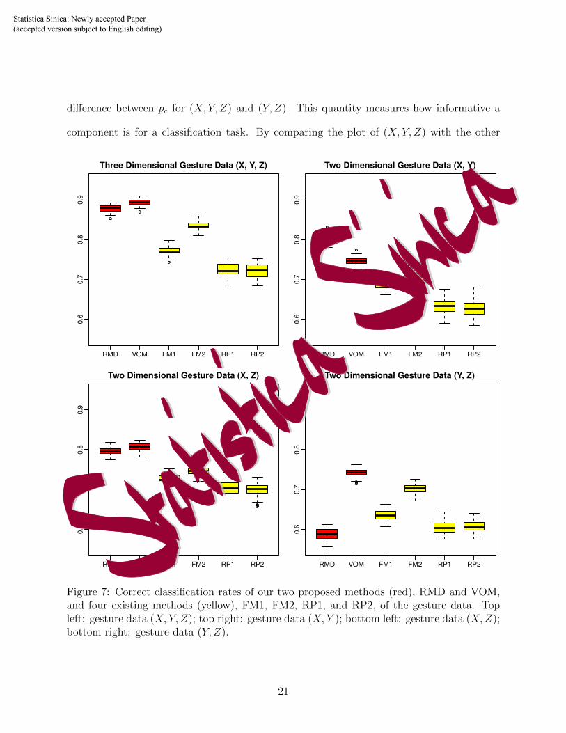
difference between pc for (X, Y, Z) and (Y, Z). This quantity measures how informative a

component is for a classification task. By comparing the plot of (X, Y, Z) with the other


0.6

0.7

0.8

0.9

Three Dimensional Gesture Data (X, Y, Z)


0.6

0.7

0.8

0.9

Two Dimensional Gesture Data (X, Y)


0.6

0.7

0.8

0.9

Two Dimensional Gesture Data (X, Z)


0.6

0.7

0.8

0.9

Two Dimensional Gesture Data (Y, Z)

Figure 7: Correct classification rates of our two proposed methods (red), RMD and VOM,and four existing methods (yellow), FM1, FM2, RP1, and RP2, of the gesture data. Topleft: gesture data (X, Y, Z); top right: gesture data (X, Y ); bottom left: gesture data (X,Z);bottom right: gesture data (Y, Z).

21


three cases, we find that the marginal effect of Y is the smallest. This finding is consistent

with the fact that the acceleration curves in direction Y are more alike with each other. For

example, the black and yellow curves in the middle graph of Figure 6 are quite similar to

the purple and red curves, respectively. In contrast, the shapes of the acceleration curves

in the other two directions differ, which leads to their higher marginal effects. The gestures

included in the dataset were mainly collected from the screens of smart phones, which means

that the direction orthogonal to the screen is not as informative as the other two directions.

5 Conclusion

In this paper, we introduced two classifiers for multivariate functional data based on di-

rectional outlyingness and the outlyingness matrix. Unlike point-type data that can be

classified only by their locations, functional data often differ not by their magnitudes but by

their shapes. This feature challenges the classifiers based on conventional functional depth

because they cannot effectively describe the shape variation between curves. Directional

outlyingness tackles this challenge by combining the direction of outlyingness with conven-

tional functional depth: it measures shape variation not only by the change in the level of

outlyingness but also by the rotation of the direction of outlyingness. For multivariate cases,

we defined the outlyingness matrix and investigated theoretical results for this matrix. On

both univariate and multivariate functional data, we evaluated our proposed classifiers and

obtained better results than existing methods using both simulated and real data.

The proposed methods can be simply generalized to image or video data (Genton et al.,

2014), where the support of functional data is two-dimensional. We plan to investigate more

general settings for both classifiers and data structures. Rather than the constant weight

22


function considered in the current paper, we believe that a weight function proportional to

local variation could further improve our methods. It is reasonable to put more weight on

the time points where the curves differ a lot and less weight on those where the curves are

quite alike. For functional data observed at irregular or sparse time points (Lopez-Pintado

and Wei, 2011), we may fit the trajectories with a set of basis functions and then estimate

depth of the discrete curves based on their continuous estimates. The functional data within

each group could be correlated in general data structures. An example is spatio-temporal

precipitation (Sun and Genton, 2012). Our methods need further modifications to account

for the correlations between functional observations as well.

Acknowledgment

The authors thank the editor, the associate editor and the two referees for their constructive

comments that led to a substantial improvement of the paper. The work of Wenlin Dai and

Marc G. Genton was supported by King Abdullah University of Science and Technology

(KAUST).

Supplementary Material

Supplementary material includes an illustrative example of functional directional outlying-

ness framework, two figures of real functional data, and technical proofs for the theoretical

results.

References

Alonso, A. M., Casado, D., and Romo, J. (2012), “Supervised classification for functional

data: A weighted distance approach,” Computational Statistics & Data Analysis, 56, 2334–

23


2346.

Apanasovich, T. V., Genton, M. G., and Sun, Y. (2012), “A valid Matern class of cross-

covariance functions for multivariate random fields with any number of components,”

Journal of the American Statistical Association, 107, 180–193.

Boser, B. E., Guyon, I. M., and Vapnik, V. N. (1992), “A training algorithm for optimal mar-

gin classifiers,” in Proceedings of the Fifth Annual Workshop on Computational Learning

Theory, ACM, pp. 144–152.

Chen, Y., Keogh, E., Hu, B., Begum, N., Bagnall, A., Mueen, A.,

and Batista, G. (2015), “The UCR Time Series Classification Archive,”

www.cs.ucr.edu/ eamonn/time series data/.

Claeskens, G., Hubert, M., Slaets, L., and Vakili, K. (2014), “Multivariate functional halfs-

pace depth,” Journal of the American Statistical Association, 109, 411–423.

Cortes, C. and Vapnik, V. (1995), “Support-vector networks,” Machine Learning, 20, 273–

297.

Cuesta-Albertos, J. A., Febrero-Bande, M., and de la Fuente, M. O. (2015), “The DDG-

classifier in the functional setting,” arXiv preprint arXiv:1501.00372.

Cuevas, A., Febrero, M., and Fraiman, R. (2007), “Robust estimation and classification for

functional data via projection-based depth notions,” Computational Statistics, 22, 481–

496.

Dai, W. and Genton, M. G. (2017), “Directional outlyingness for multivariate functional

data,” arXiv preprint arXiv:1612.04615v2.

24


Delaigle, A. and Hall, P. (2012), “Achieving near perfect classification for functional data,”

Journal of the Royal Statistical Society: Series B, 74, 267–286.

Delaigle, A., Hall, P., and Bathia, N. (2012), “Componentwise classification and clustering

of functional data,” Biometrika, 99, 299–313.

Epifanio, I. (2008), “Shape descriptors for classification of functional data,” Technometrics,

50, 284–294.

Ferraty, F. and Vieu, P. (2006), Nonparametric Functional Data Analysis: Theory and Prac-

tice, Springer.

Fraiman, R. and Muniz, G. (2001), “Trimmed means for functional data,” TEST, 10, 419–

440.

Galeano, P., Joseph, E., and Lillo, R. E. (2015), “The Mahalanobis distance for functional

data with applications to classification,” Technometrics, 57, 281–291.

Genton, M. G. and Hall, P. (2016), “A tilting approach to ranking influence,” Journal of the

Royal Statistical Society: Series B, 78, 77–97.

Genton, M. G., Johnson, C., Potter, K., Stenchikov, G., and Sun, Y. (2014), “Surface

boxplots,” Stat, 3, 1–11.

Gneiting, T., Kleiber, W., and Schlather, M. (2010), “Matern cross-covariance functions for

multivariate random fields,” Journal of the American Statistical Association, 105, 1167–

1177.

Hastie, T., Buja, A., and Tibshirani, R. (1995), “Penalized discriminant analysis,” The

Annals of Statistics, 23, 73–102.

25


Horvath, L. and Kokoszka, P. (2012), Inference for Functional Data with Applications,

Springer.

Hubert, M., Rousseeuw, P. J., and Segaert, P. (2015), “Multivariate functional outlier de-

tection,” Statistical Methods & Applications, 24, 177–202.

— (2016), “Multivariate and functional classification using depth and distance,” Advances

in Data Analysis and Classification, 1–22.

James, G. M. and Hastie, T. J. (2001), “Functional linear discriminant analysis for irregularly

sampled curves,” Journal of the Royal Statistical Society: Series B, 63, 533–550.

Kuhnt, S. and Rehage, A. (2016), “An angle-based multivariate functional pseudo-depth for

shape outlier detection,” Journal of Multivariate Analysis, 146, 325–340.

Li, B. and Yu, Q. (2008), “Classification of functional data: A segmentation approach,”

Computational Statistics & Data Analysis, 52, 4790–4800.

Li, J., Cuesta-Albertos, J. A., and Liu, R. Y. (2012), “DD-classifier: Nonparametric clas-

sification procedure based on DD-plot,” Journal of the American Statistical Association,

107, 737–753.

Li, P.-L., Chiou, J.-M., and Shyr, Y. (2017), “Functional data classification using covariate-

adjusted subspace projection,” Computational Statistics & Data Analysis, 115, 21–34.

Liu, R. Y., Parelius, J. M., and Singh, K. (1999), “Multivariate analysis by data depth:

descriptive statistics, graphics and inference,” The Annals of Statistics, 27, 783–858.

Lopez-Pintado, S. and Romo, J. (2006), “Depth-based classification for functional data,”

26


DIMACS Series in Discrete Mathematics and Theoretical Computer Science. Data Depth:

Robust Multivariate Analysis, Computational Geometry and Applications., 72, 103–120.

— (2009), “On the concept of depth for functional data,” Journal of the American Statistical

Association, 104, 718–734.

— (2011), “A half-region depth for functional data,” Computational Statistics & Data Anal-

ysis, 55, 1679–1695.

Lopez-Pintado, S., Sun, Y., Lin, J. K., and Genton, M. G. (2014), “Simplicial band depth for

multivariate functional data,” Advances in Data Analysis and Classification, 8, 321–338.

Lopez-Pintado, S. and Wei, Y. (2011), “Depth for sparse functional data,” in Ferraty F. (ed)

Recent Advances in Functional Data Analysis and Related Topics, Springer, pp. 209–212.

Mahalanobis, P. C. (1936), “On the generalized distance in statistics,” Proceedings of the

National Institute of Sciences of India, 2, 49–55.

Matern, B. (1960), Spatial Variation, Springer.

Mosler, K. and Mozharovskyi, P. (2015), “Fast DD-classification of functional data,” Statis-

tical Papers, 1–35.

Narisetty, N. N. and Nair, V. N. (2016), “Extremal depth for functional data and applica-

tions,” Journal of the American Statistical Association, 111, 1705–1714.

Ramsay, J. O. and Silverman, B. W. (2006), Functional Data Analysis, Springer.

Rossi, F. and Villa, N. (2006), “Support vector machine for functional data classification,”

Neurocomputing, 69, 730–742.

27


Rousseeuw, P. J. (1985), “Multivariate estimation with high breakdown point,” in Mathe-

matical Statistics and Applications, Volume B (W. Grossmann, G. Pflug, I. Vincze and

W. Wert, eds.), Reidel, Dordrecht, pp. 283–297.

Sguera, C., Galeano, P., and Lillo, R. (2014), “Spatial depth-based classification for func-

tional data,” TEST, 23, 725–750.

Shokoohi-Yekta, M., Hu, B., Jin, H., Wang, J., and Keogh, E. (2017), “Generalizing dynamic

time warping to the multi-dimensional case requires an adaptive approach,” Data Mining

and Knowledge Discovery, 31, 1–31.

Sun, Y. and Genton, M. G. (2011), “Functional boxplots,” Journal of Computational and

Graphical Statistics, 20, 316–334.

— (2012), “Adjusted functional boxplots for spatio-temporal data visualization and outlier

detection,” Environmetrics, 23, 54–64.

Tukey, J. W. (1975), “Mathematics and the picturing of data,” in Proceedings of the Inter-

national Congress of Mathematicians, vol. 2, pp. 523–531.

Yao, F., Wu, Y., and Zou, J. (2016), “Probability-enhanced effective dimension reduction

for classifying sparse functional data,” TEST, 25, 1–22.

Zuo, Y. (2003), “Projection-based depth functions and associated medians,” The Annals of

Statistics, 31, 1460–1490.

Zuo, Y. and Serfling, R. (2000), “General notions of statistical depth function,” The Annals

of Statistics, 28, 461–482.

28


Statistica Sinica Preprint No: SS-2016-0537

Documents

Transcript of Statistica Sinica Preprint No: SS-2016-0537