Japanese VLBI programs, East Asian VLBI Network and Space VLBI;VSOP-2
Upload
abner-austinCategory
view
225download
8
(Station Dependent) Correlation in VLBI Observations
John M. GipsonNVI, Inc./NASA GSFC
4th IVS General Meeting 9-11 January 2006Concepcion, Chile
Agenda
• Quick review of observations and formal errors in VLBI• Evidence for (unmodeled) station-dependent delay• Sources of station-dependent delay• Handling station-dependent delay• Results• Conclusions
Independence of Observations
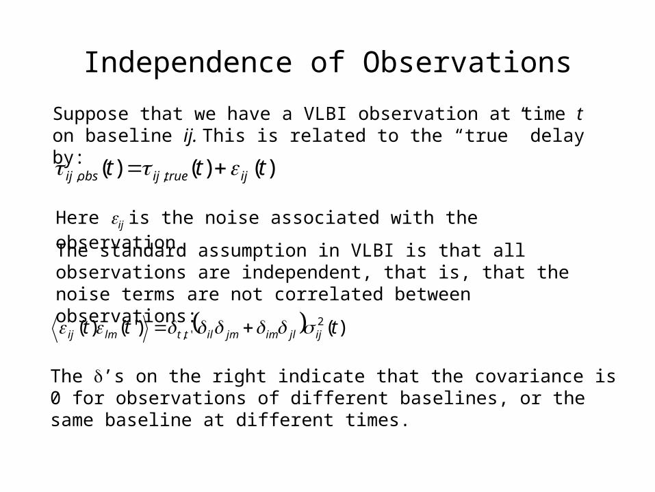
)()()( ,, ttt ijtrueijobsij
The standard assumption in VLBI is that all observations are independent, that is, that the noise terms are not correlated between observations:
Suppose that we have a VLBI observation at time t on baseline ij. This is related to the “true” delay by:
The ’s on the right indicate that the covariance is 0 for observations of different baselines, or the same baseline at different times.
)()'()( 2', ttt ijjlimjmilttlmij
Here ij is the noise associated with the observation.

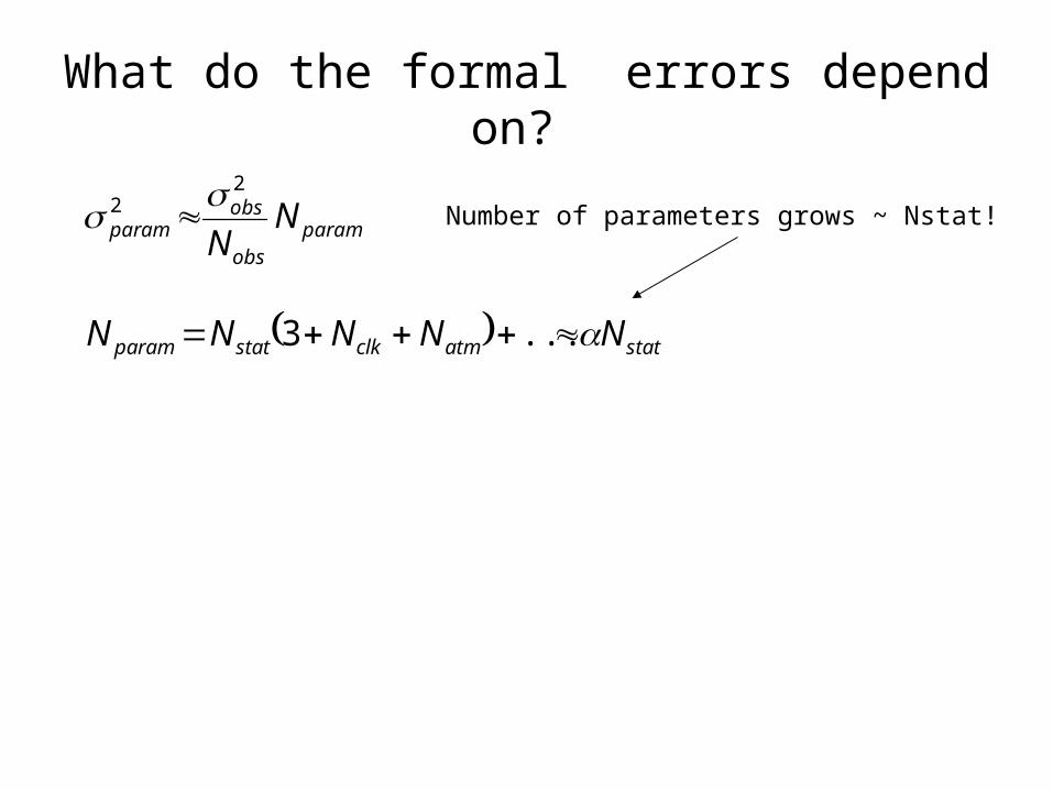
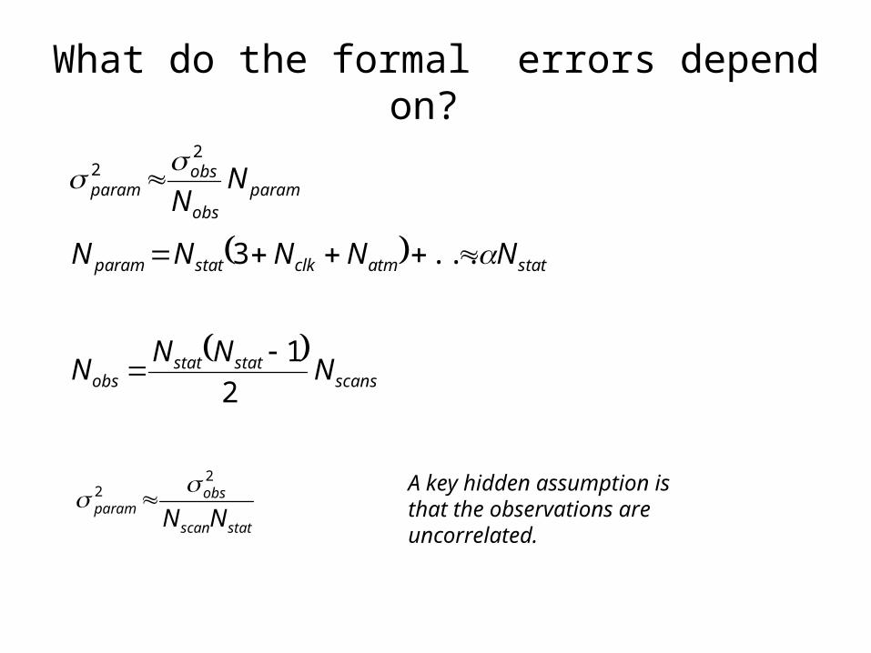
What do the formal errors depend on?
paramobs
obsparam N
N
22
What do the formal errors depend on?
paramobs
obsparam N
N
22
statatmclkstatparam NNNNN ...3
Number of parameters grows ~ Nstat!
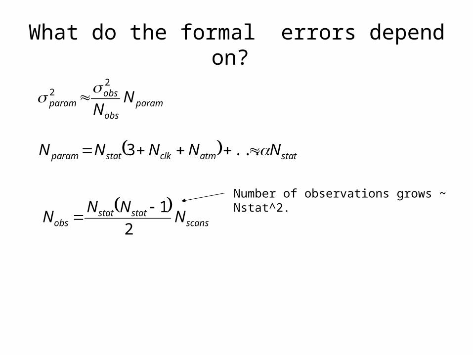
What do the formal errors depend on?
paramobs
obsparam N
N
22
scans
statstatobs N
NNN
2
1
statatmclkstatparam NNNNN ...3
Number of observations grows ~ Nstat^2.
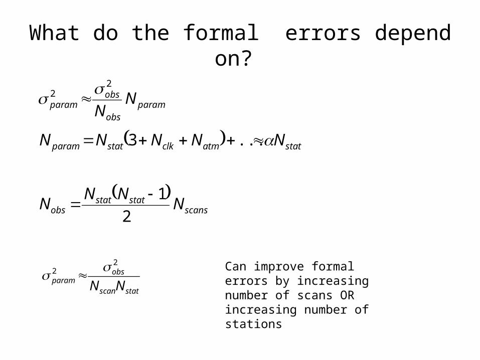
What do the formal errors depend on?
paramobs
obsparam N
N
22
scans
statstatobs N
NNN
2
1
statatmclkstatparam NNNNN ...3
statscan
obsparam NN
22
Can improve formal errors by increasing number of scans OR increasing number of stations
What do the formal errors depend on?
paramobs
obsparam N
N
22
scans
statstatobs N
NNN
2
1
statatmclkstatparam NNNNN ...3
statscan
obsparam NN
22
A key hidden assumption is that the observations are uncorrelated.
Are the observations independent? Is observational noise uncorrelated?
•We do not have direct access to the observation noise term ij. •We need to approach study of correlation indirectly.•Use the residuals to a solution (=ij) as a proxy for ij.
My approach: Look at the residuals to the solution of an RDV experiment to see if they are correlated.
RDVs have many observations, and many large net-work scans. This makes uncovering correlations easier.
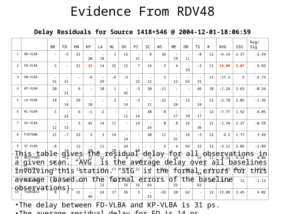
Evidence From RDV48
Delay Residuals for Source 1418+546 @ 2004-12-01-18:06:59 BR FD HN KP LA NL OV PI SC WS ME ON TS # AVG SIG Avg/Sig
1 BR-VLBA - -5 31 -20 -18 1 12 -21 8 36 -19 -11 -8 12 -6.14 2.37 -2.59
2 FD-VLBA 5 - 31 31 14 22 15 7 16 2 4 -39 -3 12 14.09 2.07 6.82
3 HN-VLBA -31 -31 - -6 -29 -6 -5 -22 -12 2 -12 -63 -31 12 -17.2 3 -5.73
4 KP-VLBA 20 -31 6 - 10 1 -45 -3 20 -11 - - 46 10 -1.24 3.63 -0.34
5 LA-VLBA 18 -14 29 -10 - 2 -14 -3 -11 -22 -24 12 -24 12 -2.78 2.05 -1.36
6 NL-VLBA -1 -22 6 -1 -2 - -11 -14 20 -8 -17 -39 -17 12 -7.77 1.92 -4.05
7 OV-VLBA -12 -15 5 45 14 11 - 14 -24 0 8 16 -36 12 -1.34 2.27 -0.59
8 PIETOWN 21 -7 22 3 3 14 -14 - 20 11 -21 16 -3 12 6.2 1.77 3.49
9 SC-VLBA -8 -16 12 -20 11 -20 24 -20 - 6 4 64 23 12 -3.11 2.86 -1.09
10 WESTFORD -36 -2 -2 11 22 8 0 -11 -6 - 34 - 32 11 0.24 4.34 0.06
11 MEDICINA 19 -4 12 - 24 17 -8 21 -4 -34 - 55 -28 11 2.81 4.31 0.65
12 ONSALA60 11 39 63 - -12 39 -16 -16 -64 - -55 - -62 10 -13.6 12 -1.13
13 TSUKUB32 8 3 31 -46 24 17 36 3 -23 -32 28 62 - 12 13.88 3.45 4.02
This table gives the residual delay for all observations in a given scan. “AVG” is the average delay over all baselines involving this station. “SIG” is the formal errors for this average (based on the formal errors of the baseline observations).
•The delay between FD-VLBA and KP-VLBA is 31 ps. •The average residual delay for FD is 14 ps•For FD the formal error is 2 ps.
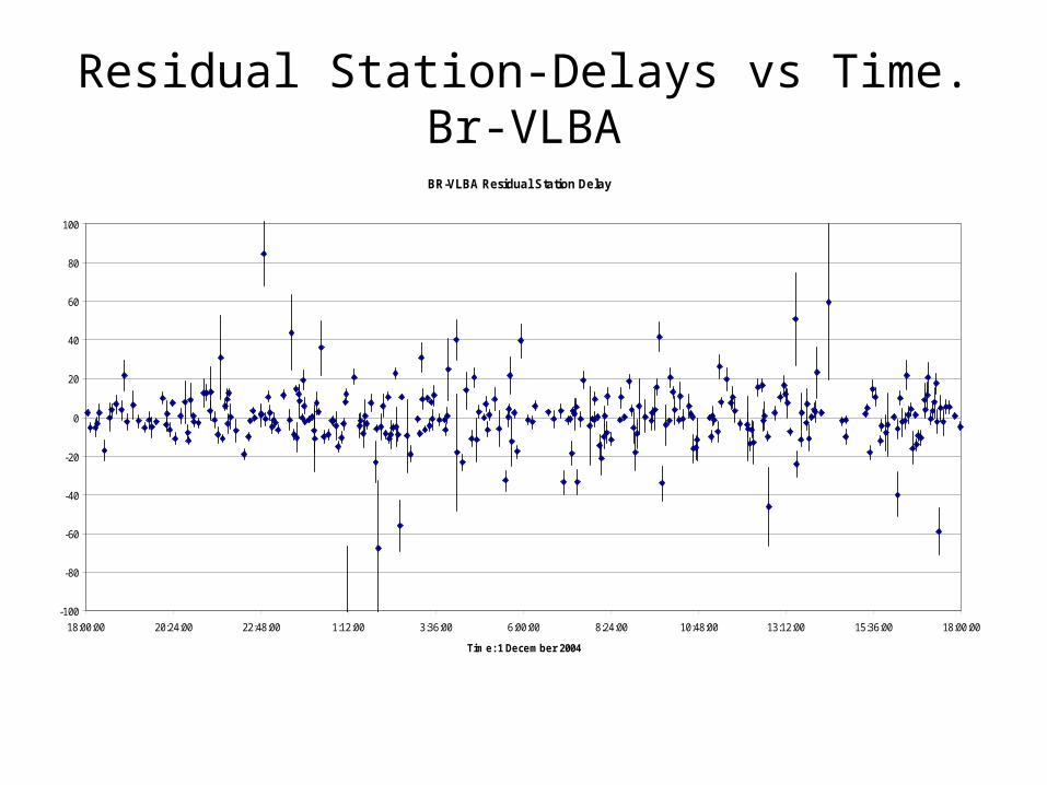
Residual Station-Delays vs Time. Br-VLBA
BR-VLBA Residual Station Delay
-100
-80
-60
-40
-20
0
20
40
60
80
100
18:00:00 20:24:00 22:48:00 1:12:00 3:36:00 6:00:00 8:24:00 10:48:00 13:12:00 15:36:00 18:00:00
Time: 1 December 2004
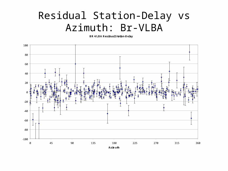
Residual Station-Delay vs Azimuth: Br-VLBABR-VLBA Residual Station-Delay
-100
-80
-60
-40
-20
0
20
40
60
80
100
0 45 90 135 180 225 270 315 360
Azimuth

Residual Station-Delay vs Elevation: BR-VLBA
BR-VLBA Residual Station-Delay
-100
-80
-60
-40
-20
0
20
40
60
80
100
0 10 20 30 40 50 60 70 80 90
Elevation
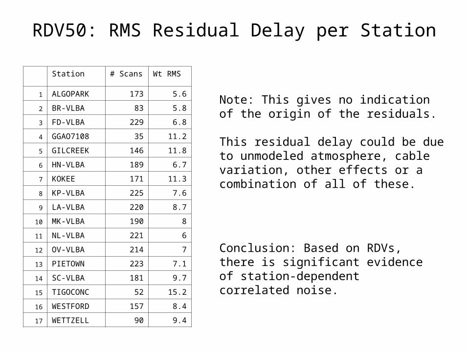
RDV50: RMS Residual Delay per Station
Station # Scans Wt RMS
1 ALGOPARK 173 5.6
2 BR-VLBA 83 5.8
3 FD-VLBA 229 6.8
4 GGAO7108 35 11.2
5 GILCREEK 146 11.8
6 HN-VLBA 189 6.7
7 KOKEE 171 11.3
8 KP-VLBA 225 7.6
9 LA-VLBA 220 8.7
10 MK-VLBA 190 8
11 NL-VLBA 221 6
12 OV-VLBA 214 7
13 PIETOWN 223 7.1
14 SC-VLBA 181 9.7
15 TIGOCONC 52 15.2
16 WESTFORD 157 8.4
17 WETTZELL 90 9.4
Note: This gives no indication of the origin of the residuals.
This residual delay could be due to unmodeled atmosphere, cable variation, other effects or a combination of all of these.
Conclusion: Based on RDVs, there is significant evidence of station-dependent correlated noise.
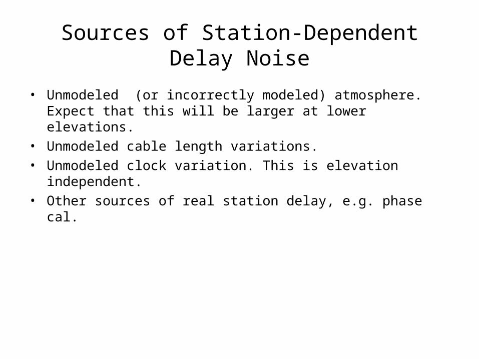
Sources of Station-Dependent Delay Noise
• Unmodeled (or incorrectly modeled) atmosphere. Expect that this will be larger at lower elevations.
• Unmodeled cable length variations. • Unmodeled clock variation. This is elevation independent.• Other sources of real station delay, e.g. phase cal.
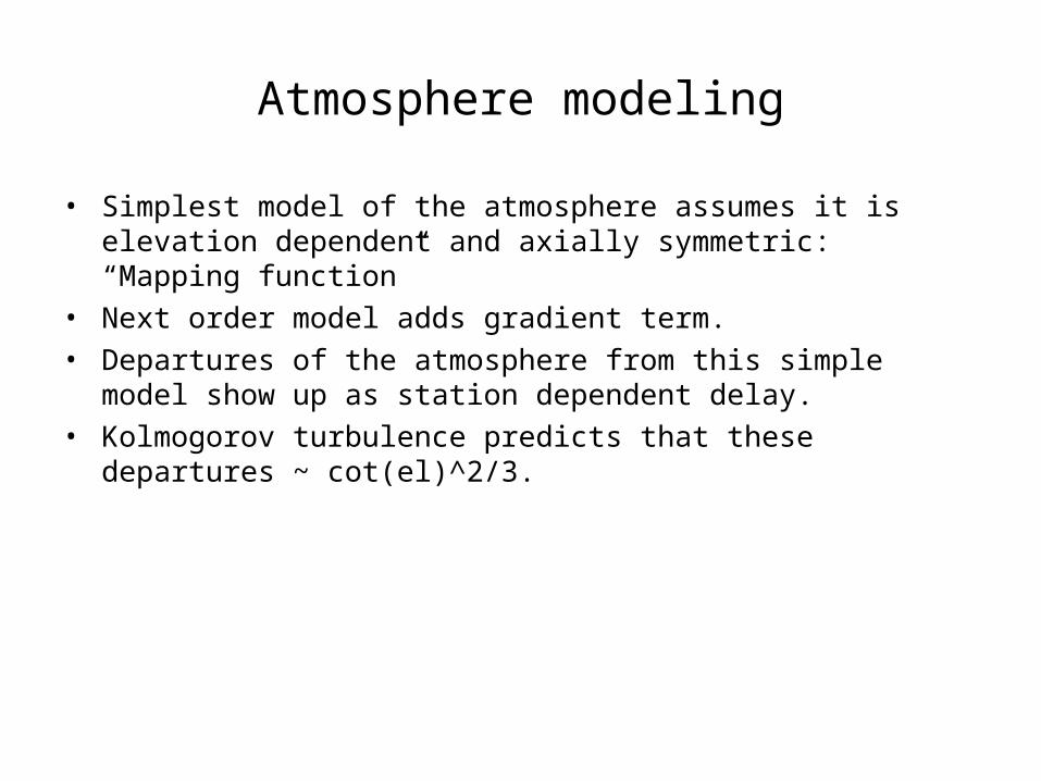
Atmosphere modeling
• Simplest model of the atmosphere assumes it is elevation dependent and axially symmetric: “Mapping function”
• Next order model adds gradient term.• Departures of the atmosphere from this simple model show up as
station dependent delay.• Kolmogorov turbulence predicts that these departures ~ cot(el)^2/3.
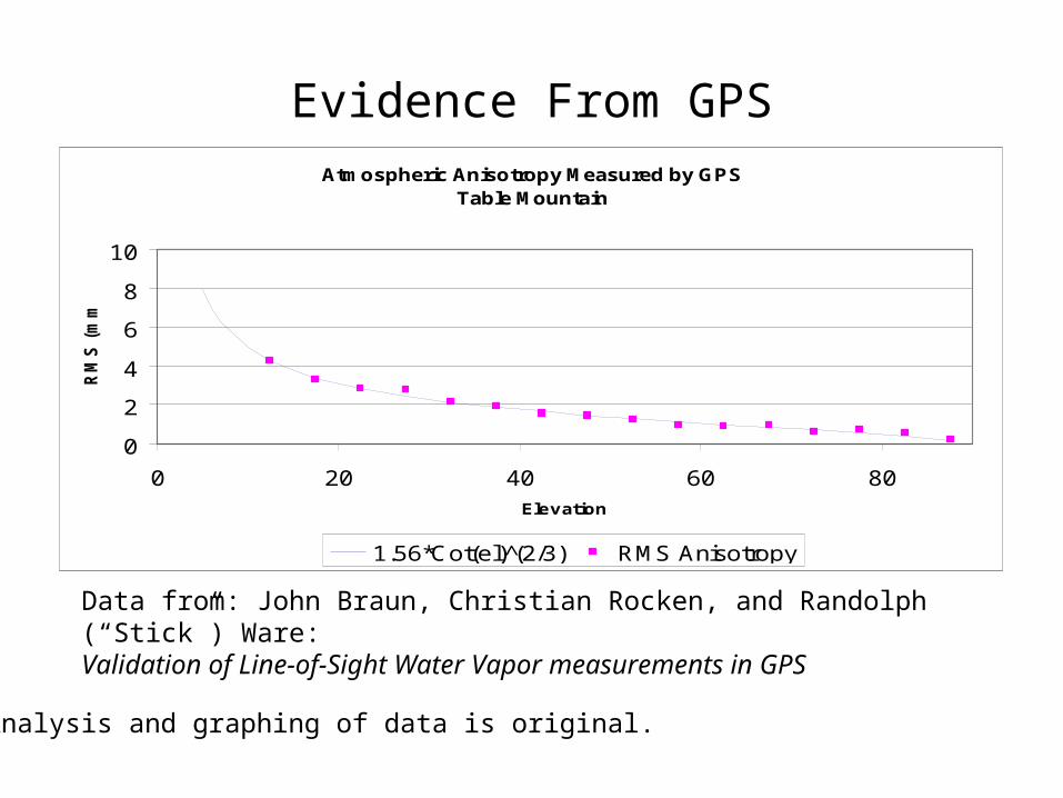
Atmospheric Anisotropy Measured by GPSTable Mountain
0
2
4
6
8
10
0 20 40 60 80
Elevation
RM
S (
mm
)
1.56*Cot(el) (̂2/3) RMS Anisotropy
Data from: John Braun, Christian Rocken, and Randolph (“Stick”) Ware:Validation of Line-of-Sight Water Vapor measurements in GPS
Analysis and graphing of data is original.
Evidence From GPS
Modeling Station-Dependent Delay
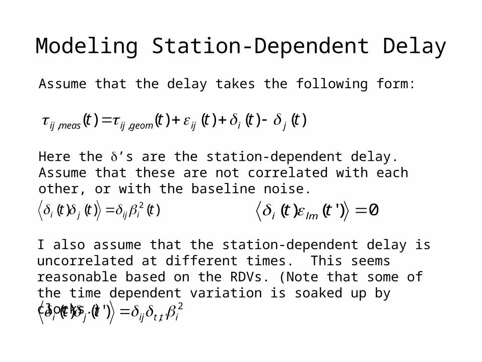
)()()( 2 ttt iijji
)()()()()( ,, ttttt jiijgeomijmeasij
Assume that the delay takes the following form:
0)'()( tt lmi
I also assume that the station-dependent delay is uncorrelated at different times. This seems reasonable based on the RDVs. (Note that some of the time dependent variation is soaked up by clocks.)
2',)'()( ittijji tt
Here the ’s are the station-dependent delay. Assume that these are not correlated with each other, or with the baseline noise.
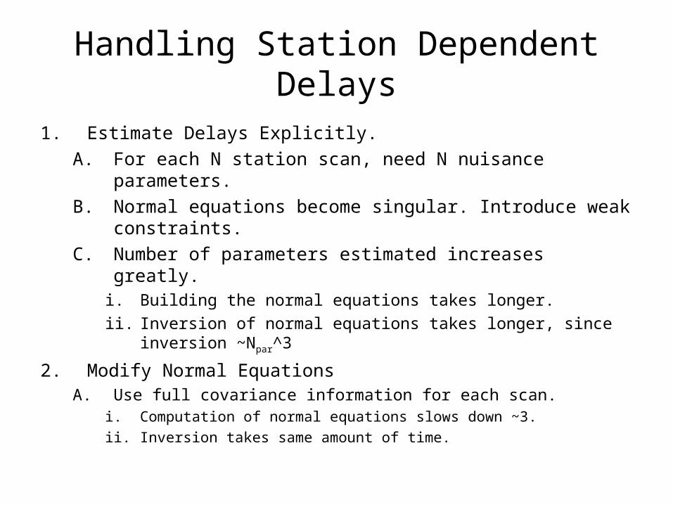
Handling Station Dependent Delays
1. Estimate Delays Explicitly.
A. For each N station scan, need N nuisance parameters.
B. Normal equations become singular. Introduce weak constraints.
C. Number of parameters estimated increases greatly. i. Building the normal equations takes longer.
ii. Inversion of normal equations takes longer, since inversion ~Npar^3
2. Modify Normal EquationsA. Use full covariance information for each scan.
i. Computation of normal equations slows down ~3.
ii. Inversion takes same amount of time.
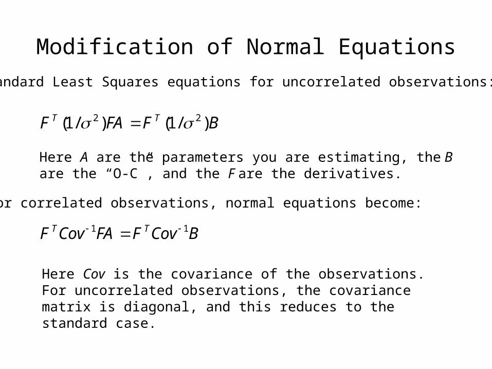
Modification of Normal Equations
BCovFFACovF TT 11
Standard Least Squares equations for uncorrelated observations:
For correlated observations, normal equations become:
BFFAF TT )/1()/1( 22
Here A are the parameters you are estimating, the B are the “O-C”, and the F are the derivatives.
Here Cov is the covariance of the observations. For uncorrelated observations, the covariance matrix is diagonal, and this reduces to the standard case.
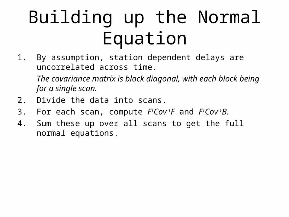
Building up the Normal Equation
1. By assumption, station dependent delays are uncorrelated across time.
The covariance matrix is block diagonal, with each block being for a single scan.
2. Divide the data into scans.
3. For each scan, compute FTCov-1F and FTCov-1B.
4. Sum these up over all scans to get the full normal equations.
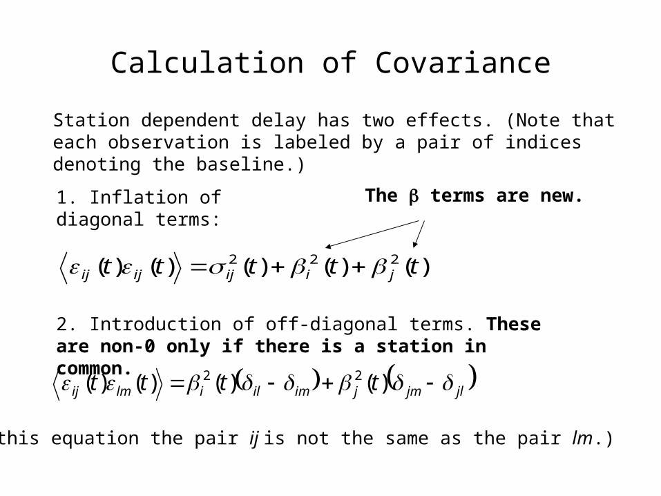
Calculation of Covariance
)()()()()( 222 ttttt jiijijij
1. Inflation of diagonal terms:
2. Introduction of off-diagonal terms. These are non-0 only if there is a station in common.
jljmjimililmij tttt )()()()( 22
(In this equation the pair ij is not the same as the pair lm.)
Station dependent delay has two effects. (Note that each observation is labeled by a pair of indices denoting the baseline.)
The terms are new.
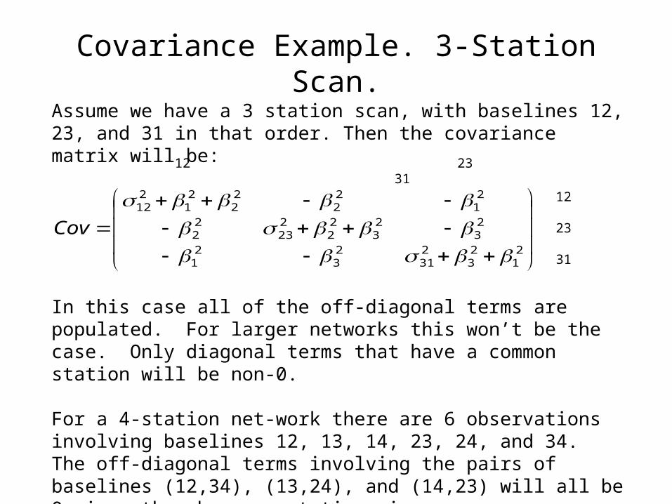
Covariance Example. 3-Station Scan.
2
123
231
23
21
23
23
22
223
22
21
22
22
21
212
Cov
Assume we have a 3 station scan, with baselines 12, 23, and 31 in that order. Then the covariance matrix will be:
In this case all of the off-diagonal terms are populated. For larger networks this won’t be the case. Only diagonal terms that have a common station will be non-0.
For a 4-station net-work there are 6 observations involving baselines 12, 13, 14, 23, 24, and 34. The off-diagonal terms involving the pairs of baselines (12,34), (13,24), and (14,23) will all be 0 since they have no stations in common.
12 23 31
12
23
31
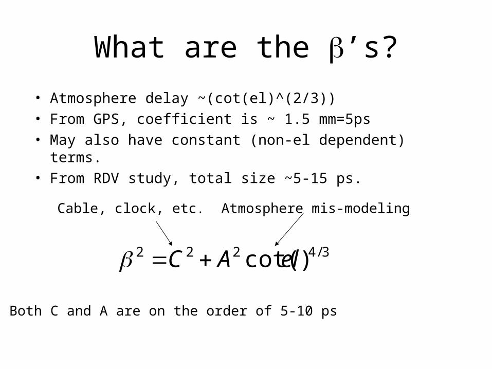
What are the ’s?
• Atmosphere delay ~(cot(el)^(2/3))• From GPS, coefficient is ~ 1.5 mm=5ps• May also have constant (non-el dependent) terms.• From RDV study, total size ~5-15 ps.
3/4222 )cot(elAC
Atmosphere mis-modelingCable, clock, etc.
Both C and A are on the order of 5-10 ps
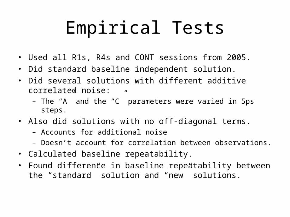
Empirical Tests
• Used all R1s, R4s and CONT sessions from 2005.• Did standard baseline independent solution.• Did several solutions with different additive correlated noise:
– The “A” and the “C” parameters were varied in 5ps steps.
• Also did solutions with no off-diagonal terms.– Accounts for additional noise
– Doesn’t account for correlation between observations.
• Calculated baseline repeatability.• Found difference in baseline repeatability between the “standard”
solution and “new” solutions.
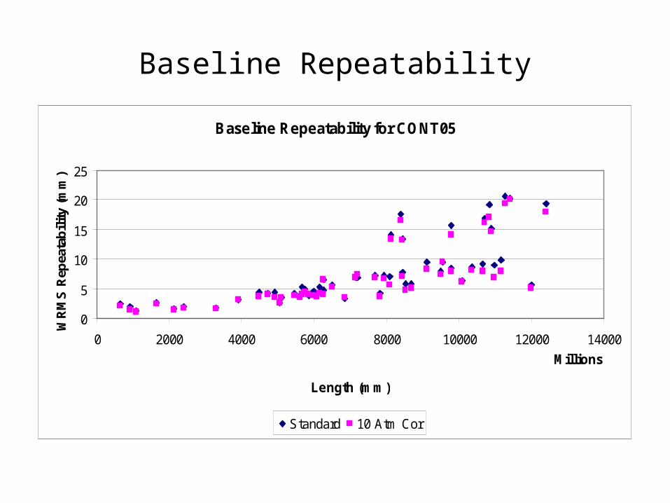
Baseline Repeatability
Baseline Repeatability for CONT05
0
5
10
15
20
25
0 2000 4000 6000 8000 10000 12000 14000
Millions
Length (mm)
WR
MS
Rep
eata
bil
ity
(mm
)
Standard 10 Atm Cor
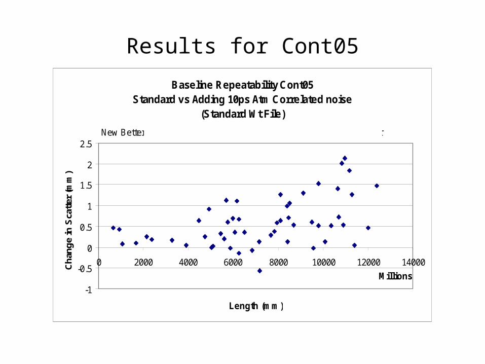
Results for Cont05
Baseline Repeatability Cont05Standard vs Adding 10ps Atm Correlated noise
(Standard Wt File)
-1
-0.5
0
0.5
1
1.5
2
2.5
0 2000 4000 6000 8000 10000 12000 14000
Millions
Length (mm)
Ch
ang
e in
Sca
tter
(m
m)
New Better
Standard Better
48/54 betterAverage improvement 0.58 mm
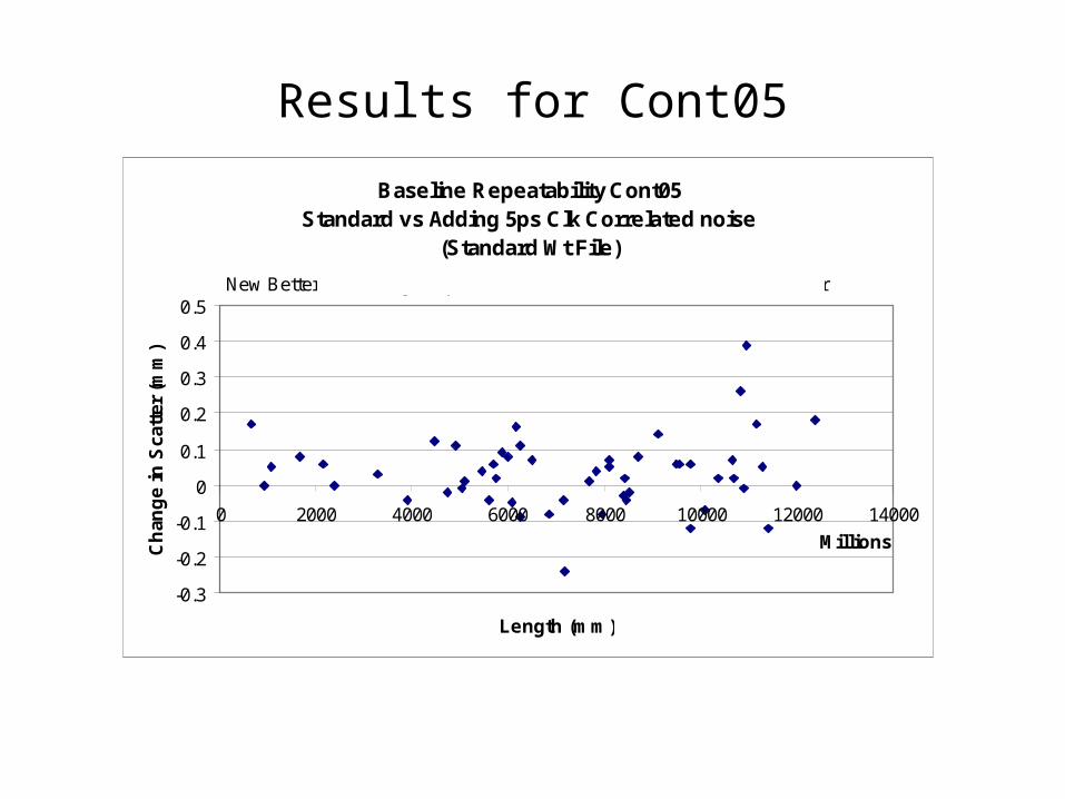
Results for Cont05
Baseline Repeatability Cont05Standard vs Adding 5ps Clk Correlated noise
(Standard Wt File)
-0.3
-0.2
-0.1
0
0.1
0.2
0.3
0.4
0.5
0 2000 4000 6000 8000 10000 12000 14000
Millions
Length (mm)
Ch
ang
e in
Sca
tter
(m
m)
New Better
Standard Better
34/54 betterAverage improvement 0.04 mm
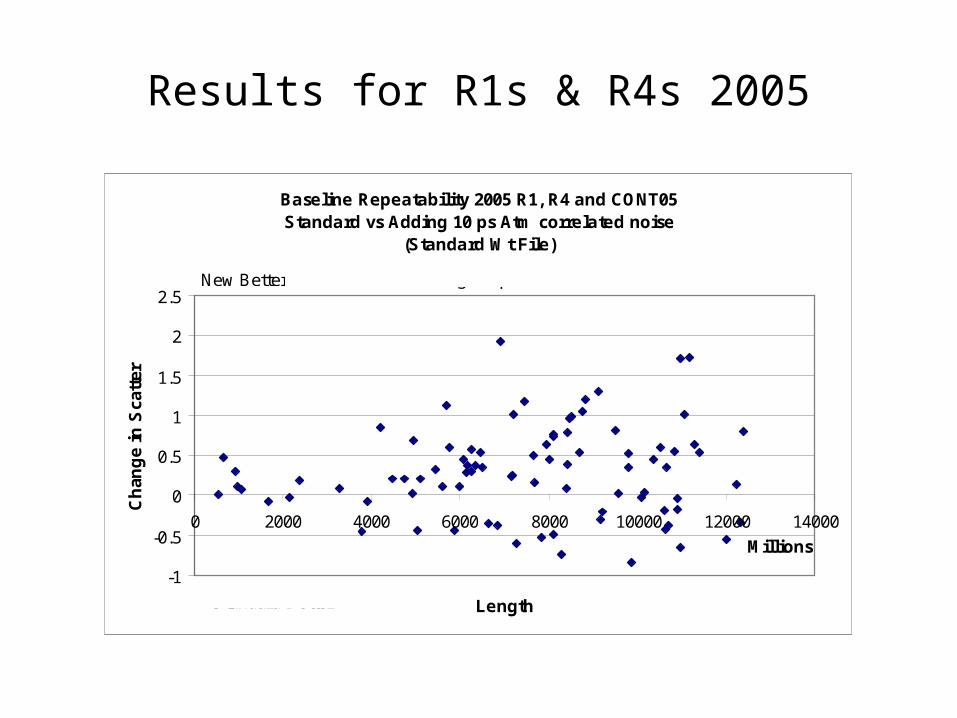
Results for R1s & R4s 2005
Baseline Repeatability 2005 R1, R4 and CONT05Standard vs Adding 10 ps Atm correlated noise
(Standard Wt File)
-1
-0.5
0
0.5
1
1.5
2
2.5
0 2000 4000 6000 8000 10000 12000 14000
Millions
Length
Ch
ang
e in
Sca
tter
New Better
Standard Better
61/84 betterAverage improvement 0.30 mm
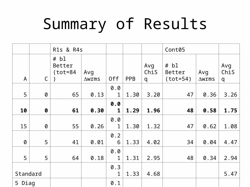
Summary of Results
R1s & R4s Cont05
A C# bl Better (tot=84)
Avgwrms Off PPB
Avg ChiSq
# bl Better (tot=54)
Avgwrms
Avg ChiSq
5 0 65 0.13 0.01 1.30 3.20 47 0.36 3.26
10 0 61 0.30 0.01 1.29 1.96 48 0.58 1.75
15 0 55 0.26 0.01 1.30 1.32 47 0.62 1.08
0 5 41 0.01 0.26 1.33 4.02 34 0.04 4.47
5 5 64 0.18 0.01 1.31 2.95 48 0.34 2.94
Standard 0.31 1.33 4.68 5.47
5 Diag Atm 62 0.09 0.13 1.32 3.72
10 Diag Atm 57 0.13 0.01 1.32 2.56
15 Diag Atm 53 0.10 0.01 1.32 1.82
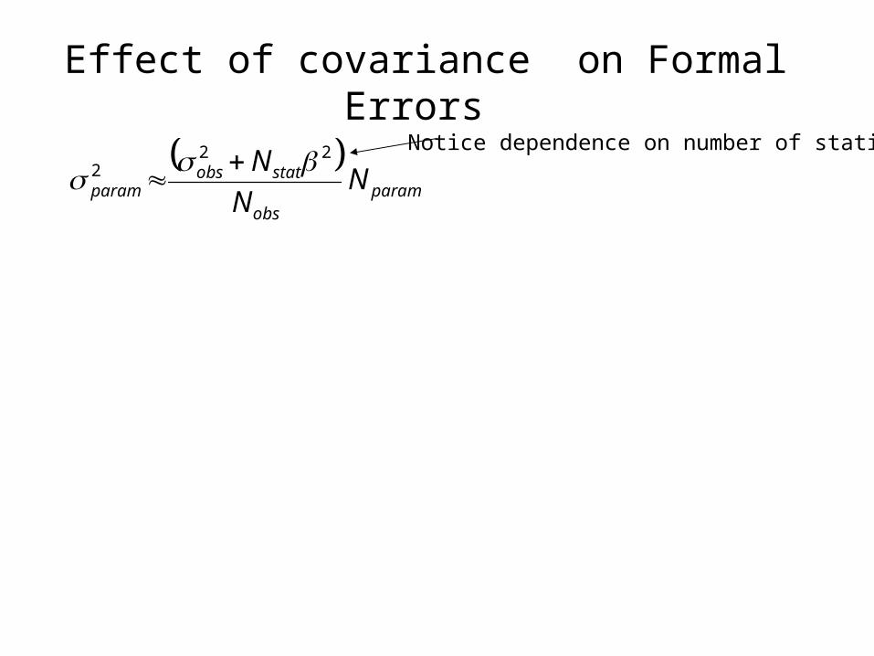
Effect of covariance on Formal Errors
param
obs
statobsparam N
N
N 222
Notice dependence on number of stations
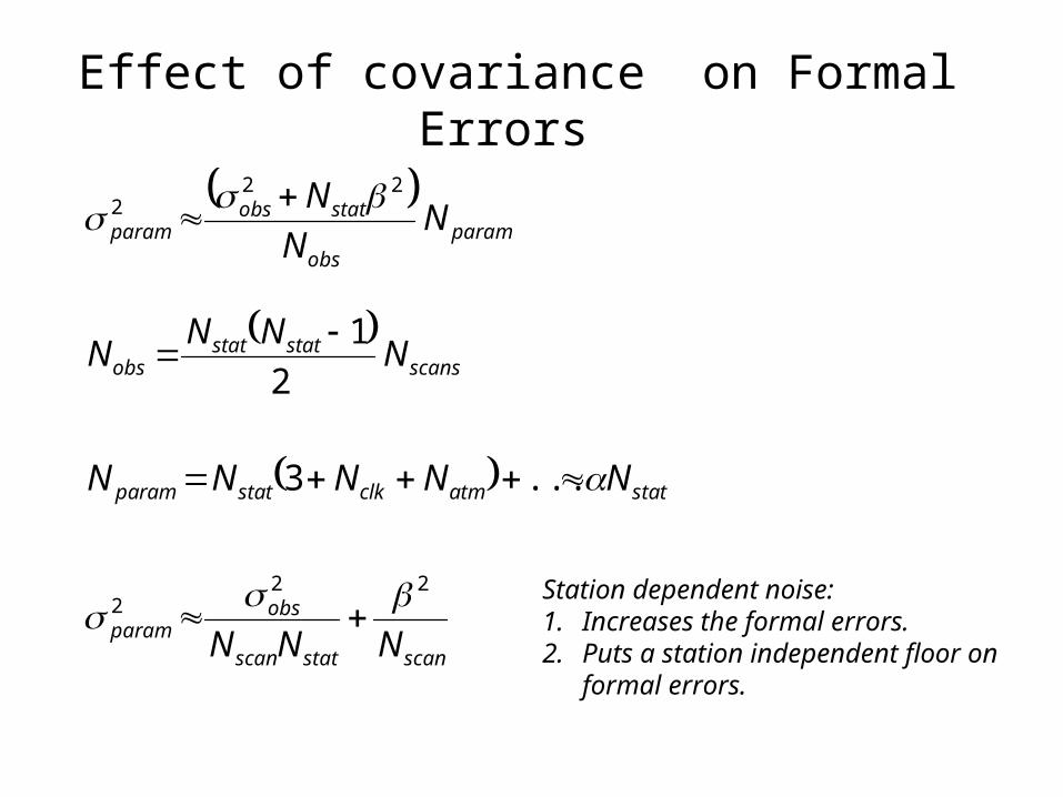
Effect of covariance on Formal Errors
param
obs
statobsparam N
N
N 222
scans
statstatobs N
NNN
2
1
statatmclkstatparam NNNNN ...3
scanstatscan
obsparam NNN
222
Station dependent noise:1. Increases the formal errors.2. Puts a station independent floor on
formal errors.
Conclusions
1. Clear evidence from RDVs that there is unmodeled station dependent delay noise terms.
2. GPS data indicates the presence of unmodeled atmosphere delay.
3. There may be other sources of delay as well: cable, clocks, etc.
4. Accounting for the correlation:A. Reduces baseline scatter.
B. Makes the formal errors more realistic.
5. In VLBI, most of the unmodeled-station-dependent-delay appears to be “atmosphere like”.
6. Reduction in scatter is not due to down-weighting the data: correlation between observations is necessary.