Static Magnetic Fields (PDF, 1.5 MB) - Health Protection Agency
156
Static Magnetic Fields Report of the independent Advisory Group on Non-ionising Radiation
Transcript of Static Magnetic Fields (PDF, 1.5 MB) - Health Protection Agency
Static Magnetic Fields
Report of the independent Advisory Group on Non-ionising Radiation


RCE-6
Static Magnetic Fields
Report of the independent Advisory Group on Non-ionising Radiation
Documents of the Health Protection Agency Radiation, Chemical and Environmental Hazards May 2008

iii
Contents
Foreword v Advisory Group on Non-ionising Radiation Membership vii
Static Magnetic Fields 1 Executive Summary 3
1 Introduction 5
2 Sources, Exposures and Measurements 8 2.1 Quantities and units 8 2.2 Magnetic environment 9 2.3 Magnetic resonance imaging 12 2.4 Other static magnetic field sources 20 2.5 Measurement equipment 28 2.6 Summary and conclusions 31 2.7 References 32
3 Mechanisms for Biological Interaction 35 3.1 Electrodynamic interactions 35 3.2 Magnetomechanical interactions 37 3.3 Electrodynamic interactions in body tissue 38 3.4 Magnetomechanical interactions in body tissue 46 3.5 Summary and conclusions 48 3.6 References 49
4 Cellular Studies 52 4.1 Genotoxic effects 52 4.2 Changes in cellular processes 58 4.3 Orientation 60 4.4 Summary and conclusions 63 4.5 References 64
iv
5 Animal Studies 67 5.1 Cancer-related endpoints 67 5.2 Reproduction and development 69 5.3 Physiological and behavioural responses 72 5.4 Summary and conclusions 90 5.5 References 91
6 Human Exposures: Experimental Studies 97 6.1 Cardiovascular effects 97 6.2 Cognitive, neurological and sensory effects 100 6.3 References 115
7 Human Exposures: Epidemiological Studies, Randomised Trials and Case Reports 117 7.1 Cancer 117 7.2 Reproductive and developmental outcomes 120 7.3 Therapeutic trials using static magnetic fields 122 7.4 Immune function 122 7.5 Other health outcomes 126 7.6 Summary and conclusions 127 7.7 References 127
8 Conclusions 130 8.1 Sources, exposures and measurements 130 8.2 Mechanisms for biological interaction 131 8.3 Cellular studies 132 8.4 Animal studies 133 8.5 Human exposures 133
9 Research Recommendations 135 9.1 Sources, exposures and measurements 135 9.2 Mechanisms for biological interaction 136 9.3 Cellular studies 136 9.4 Animal studies 136 9.5 Human exposures 137
Glossary 139
Appendix Publications of the independent Advisory Group on Non-ionising Radiation 143
v
Foreword
The Health Protection Agency has a statutory responsibility for advising UK government departments on health effects and standards of protection for exposure to ionising and non-ionising radiations. This responsibility came to the Agency in April 2005 when it incorporated the National Radiological Protection Board (NRPB) as its Radiation Protection Division (RPD).
In 1990, to provide support for the development of advice on non-ionising radiations, the Director of the NRPB set up the Advisory Group on Non-ionising Radiation with terms of reference:
‘to review work on the biological effects of non-ionising radiation relevant to
human health and to advise on research priorities’
The Advisory Group was reconstituted in 1999 as an independent body and now reports to the subcommittee of the Board of the HPA that deals with radiation, chemical and environmental hazards. Its current membership is given on page vii of this report. For details of its work programme, see the website www.hpa.org.uk.
The Advisory Group has, to date, issued a number of reports concerned with exposures to electromagnetic fields (EMFs). It has considered
a their possible association with an increased risk of cancer, including childhood leukaemia,
b neurodegenerative disease,
c corona ions and increased particle deposition near power lines,
d melatonin, breast cancer and exposure to power frequency fields,
e health effects related to the use of visual display units,
f potential health effects of radiofrequency fields.
Details of publications by the Advisory Group are given in an appendix.
In this report the Advisory Group considers the available scientific evidence from studies of people, animals and cells relating to health effects from exposure to static magnetic fields. The report is limited to direct biological effects of static fields, and therefore does not review the evidence on two known indirect effects that can affect health – the risk of accidental injury from flying metal objects attracted by the magnet (‘the projectile effect’), and the effect of magnetic fields on implanted electrical devices and implanted metallic devices. Some emphasis is placed on static field exposures resulting from the use of magnetic resonance imaging (MRI) procedures in medical diagnosis. The report is about static magnetic fields, not MRI per se, however, and therefore does not consider other non-ionising radiation exposures from MRI.

vii
Advisory Group on Non-ionising Radiation Membership
CHAIRMAN Professor A J Swerdlow Section of Epidemiology, Institute of Cancer Research, University of London
MEMBERS Professor L J Challis University of Nottingham
Professor D N M Coggon University of Southampton
Dr L A Coulton University of Sheffield
Professor S C Darby Clinical Trials Service Unit, University of Oxford
Professor P A Gowland University of Nottingham
Professor P Haggard Institute of Cognitive Neuroscience, University College London
Professor D J Lomas Addenbrooke’s Hospital, University of Cambridge
Professor D Noble University of Oxford
SECRETARIAT Dr S M Mann Health Protection Agency, Chilton
OBSERVER Dr H Walker Department of Health, London
viii
HPA REPRESENTATIVES Dr A F McKinlay Health Protection Agency, Chilton
Dr C R Muirhead Health Protection Agency, Chilton
Dr R D Saunders Health Protection Agency, Chilton
Dr J W Stather Health Protection Agency, Chilton
CONSULTANTS Mr S G Allen Health Protection Agency, Chilton
Dr Z J Sienkiewicz Health Protection Agency, Chilton
This report from the independent Advisory Group on Non-ionising Radiation reflects understanding and evaluation of the current scientific evidence as presented and referenced in this document.
Static Magnetic Fields
Report of the independent Advisory Group on Non-ionising Radiation
Chairman: Professor A J Swerdlow

3
Executive Summary
Exposure to static magnetic fields of 25–60 microtesla (μT) from the Earth’s core is ubiquitous. In addition, greater exposures occur from certain man-made sources, produced either as a deliberate consequence or as a byproduct of the operation of electrical equipment and distribution of direct current (DC) electricity, or from permanent magnets. Certain industrial processes, including aluminium production and the chloralkali industry, involve exposures up to around 20 millitesla (mT). Particularly large exposures, of up to several tesla (T), can occur from magnetic resonance imaging (MRI) and spectroscopy, and from sources used in certain areas of scientific research. There are a number of theoretical mechanisms, via electrodynamic and magnetomechanical interactions, by which such fields might directly affect biological functioning, especially by reducing blood flow in the aorta and inducing currents in the surrounding tissue, stimulating peripheral nerves, and disturbing the functioning of the vestibular system (balance organs).
In the laboratory, certain macromolecules and cells can be shown to align in a field of about 0.5 T or more, but the implications of this are not clear. Although some changes in cellular function have been recorded in experiments at fields of 0.2 T or more, no direct adverse effects on cells of magnetic fields alone have been established.
Studies of animals have shown aversive responses in fields of about 4 T and greater, probably reflecting effects of exposure on the vestibular system. Induction of electric currents around the heart and major blood vessels of animals by magnetic fields above 100 mT has been demonstrated, but no adverse consequences were found. Studies of other biological responses in animals have been limited but have not shown any adverse effects.
At fields up to 8 T, cardiovascular effects have been observed in people but these effects have been minimal and within the range of normal physiological variation; the available data are, however, limited. Some individuals exposed to fields of about 2 T or greater experience transient sensations, including vertigo and a metallic taste in the mouth. These appear to relate at least in part to movement in the field, and can be reduced by moving more slowly. Studies of other cognitive and neurological functions in people have not given convincing evidence of any effect. Epidemiological studies and clinical case reports do not indicate any long-term adverse effects of exposures to static magnetic fields, but the data are sparse and, in particular, there have been no long-term cohort (follow-up) studies on patients and staff involved with magnetic resonance procedures.
Overall, the available evidence shows the following. At levels of static magnetic field exposure above about 2 T, transient sensory effects occur in some individuals; these effects relate at least in part to movement in the field. No serious or permanent health effects have been found from human exposures at levels up to 8 T, but scientific investigation has been limited. The effects of human exposure to fields above 8 T are unknown, but some cardiovascular and sensory effects would be expected to increase with stronger fields.

5
1 Introduction
Over recent years there has been a rapid increase in the use of technologies employing electromagnetic fields and radiations (EMFs) covering all parts of the electromagnetic spectrum. Sources of exposure include power frequency fields (50 Hz) in the national grid system, the local electricity supply network, and mains wiring in homes, offices and other buildings. In addition, all machines, appliances and devices powered by electricity, produce EMFs. There has also been a rapid expansion of technologies using radiofrequency (RF) fields. These include radio and TV transmitters, telecommunications links and satellite communication, mobile phones and their supporting base stations, as well as wireless computer networking. The Advisory Group on Non-ionising Radiation (AGNIR) has issued reports covering exposures to power frequency electric and magnetic fields, and to radiofrequency fields. In addition to time-varying fields, people may also be exposed to static magnetic and electric fields (ie fields that do not vary with time) both in medical procedures and in other situations. The number of applications is growing and the levels of exposure are known to be increasing. The present report by the AGNIR is concerned with the assessment of health effects from exposures to static magnetic fields.
To date there has been little public interest in possible adverse health effects of exposure to static magnetic fields and rather limited research. These fields are used to advantage in certain industries, high energy physics research facilities, and particularly in medicine where magnetic resonance imaging (MRI) provides exceptionally clear images of tissue that can lead to more effective diagnosis of disease or injury. There have been rapid advances in the applications of static fields and, in addition, there have been progressive increases in the strength of the magnetic fields used. In particular, in MRI it is expected that exposures of several tesla (T) may become more common while partial body exposures can be even higher.
As a consequence, the Board of the National Radiological Protection Board (NRPB), now the Radiation Protection Division (RPD) of the Health Protection Agency (HPA), asked the AGNIR to review the technologies and possible health implications of exposure to high strength static magnetic fields of patients, members of the public, and people who may be occupationally exposed.
The NRPB, together with the International Commission on Non-Ionizing Radiation Protection (ICNIRP) and the World Health Organization (WHO), held an international workshop in April 2004 to consider the health effects of exposure to intense static magnetic fields. The published proceedings reviewed current evidence on short- and long-term health effects of exposure to static fields and have been a valuable input to the work of the AGNIR.
The physical principles involved in the production of static magnetic fields are considered in Chapter 2 together with information on natural and artificial sources. Medical diagnosis using MRI and magnetic resonance spectroscopy (MRS) is the main source of high exposure of people to static fields. In 2007 around 35 machines of 3 T were expected to be operational in the UK. In addition to patients, staff and
1 I N T R O D U C T I O N
6
volunteers can also be exposed to strong static fields. The development and use of this equipment and current trends in exposures are also considered, together with information on numbers of people involved, developments in equipment and techniques, and the strength of the fields.
Chapter 3 considers mechanisms of interaction between magnetic fields and biological systems. Static magnetic fields interact with moving charged particles, such as ions, and with magnetic moments (dipoles) arising from the orbital motion or spin of electrons in an atom. Many nuclei also have moments, although these are much smaller than those associated with electrons. Electrodynamic interactions, involving charges, and magnetomechanical interactions, involving magnetic dipoles, are considered in this chapter, as is their role in causing interactions between magnetic fields and body tissues. Of particular importance is their influence on blood flow, vertigo and signalling in the nervous system.
Cellular studies are valuable for providing a method for assessing the potential effects of various agents on the human body in a well-defined and controlled way. They can be used as a screening process to analyse possible interactions of agents with body tissues and to understand mechanisms of interaction, although effects demonstrated in cells in culture are not always reflected in similar changes in the whole organism. Chapter 4 examines experimental studies on the biological effects of exposure to static magnetic fields. Various indicators of biological damage are considered including DNA damage and the induction of chromosomal aberrations, mutational change, and cellular division and proliferation, as well as changes in cellular processes including gene expression, intracellular signalling, and metabolic activity.
Further information relevant to an assessment of possible effects on health can be obtained from animal studies. These can demonstrate effects on organs and tissues as well as whole organisms. They can be carried out in a controlled and coordinated way, the dosimetry can be properly calibrated and, if necessary, exposure–response information can be obtained. Chapter 5 summarises animal studies that have been carried out to assess the possible effects of static magnetic fields on the body.
Blood flow in an applied magnetic field gives rise to induced voltages in the aorta and other major arteries of the central circulatory system that can be observed as superimposed electrical signals in the electrocardiogram (ECG). Studies involving the measurement of blood pressure, blood flow rate, heart sounds, and cardiac valve displacements have been carried out in monkeys and dogs exposed to static fields to examine the effects on cardiac function and haemodynamic parameters.
Experimental studies in people provide a direct method for examining the effects of static magnetic fields on the body. Chapter 6 considers the main studies that have been carried out to investigate the effects of static magnetic fields on cardiovascular, cognitive and neurological function. Effects of direct mechanical torque on implanted and extracorporeal metallic and electrical cardiovascular devices such as replacement cardiac valves and artificial pacemakers are well recognised but beyond the scope of this report. Potential direct biological effects of magnetic fields on the cardiovascular system have been less studied in people; the published work is reviewed in this chapter including studies of cardiac pump performance, cardiac rhythm, and vascular resistance. The presence of magnetic fields also has the potential to alter the normal function of nerve cells either peripherally in the body or centrally in the brain and spinal cord. Recent studies of the effects of magnetic fields, and particularly static magnetic fields, on the function of the human nervous system are reviewed. The range of investigations covered includes

I N T R O D U C T I O N
7
studies on nerve conduction, electroencephalography (EEG) and neuroimaging, effects on evoked potential, changes in cognitive function and brain metabolism.
Data on possible health effects from exposure to static magnetic fields are also available from epidemiological studies and clinical observations in people. The evidence examined in Chapter 7 relates to groups of people exposed at work in industrial processes that use DC supplies for electrolysis, follow-up studies of people exposed to MRI, and patients exposed to magnetic devices used in the treatment of pain. The main health outcomes examined have been the induction of cancer, reproductive and developmental disorders, and impairment of immune function.
The conclusions of the report are given in Chapter 8 and recommendations for further work are given in Chapter 9.

8
2 Sources, Exposures and Measurements
2.1 Quantities and units
Static magnetic fields are produced either by permanent magnets or by flows of direct current (DC) through conducting materials. The Biot Savart law describes how current-carrying elements produce magnetic fields such that the magnetic field contribution, dB, due to a thin wire element of length, dl, supporting a current, I, is given by
3
dd
4
r
μπ×
=r
BlI
(2.1)
where r is the vector from the location of the current element to the point where the field is calculated and μ is the permeability of the medium. This shows that the magnetic field is a vector quantity with a direction that circulates around the current element producing it and with a magnitude that decreases with the square of the distance from the current element. Integrations may be carried out using equation 2.1 to evaluate the magnetic field at any point in the space around current-carrying structures – for example, coils or electricity distribution networks.
Magnetic fields are described in terms of the force they exert on moving charges, eg those that comprise electric currents. The magnitude of the force, F, in newtons is proportional to the size of the charge, q, in coulombs and its velocity, v, in metres per second, and the direction of the force is at right angles to both the direction of motion and the field. Mathematically, this is expressed as
q= ×F v B (2.2)
The B-fields referred to above are more strictly termed magnetic flux densities and their unit is the tesla, T. Often multipliers are applied to the unit such that nT (nanotesla), μT (microtesla) and mT (millitesla) are quoted.
The true magnetic field strength has the symbol H and the unit ampere per metre (A m−1). It is closely related to the magnetic flux density through
μ=B H (2.3)
In non-magnetic materials such as air, the permeability is equal to the permeability of free space, μ0, which is by definition equal to 4π 10−7 H m−1 (henrys per metre).
Magnetic fields store energy such that the energy per unit volume (J m−3), U M, is given by
μ= 2
M / 2U B (2.4)
For example, a 1 T field stores an energy density of 400 kJ m−3.
M A G N E T I C E N V I R O N M E N T
9
It should be noted that the oersted and the gauss are the units for magnetic field strength and flux density in the now obsolete CGS system of units. The permeability of free space is unity in the CGS system, such that the field strength and flux density are equal in vacuo. The gauss is still in fairly common use and 104 gauss is equal to 1 tesla.
2.2 Magnetic environment
At the centre of the Earth is a conducting iron core in which electric currents flow, and hence give rise to a static magnetic field. The fields at the surface of the Earth have a similar structure to those from a bar magnet inclined around 11° from the Earth’s axis of rotation. The magnetic field is thus approximately parallel to the Earth’s surface at the equator and generally becomes more vertically inclined towards the north and south poles of the planet.
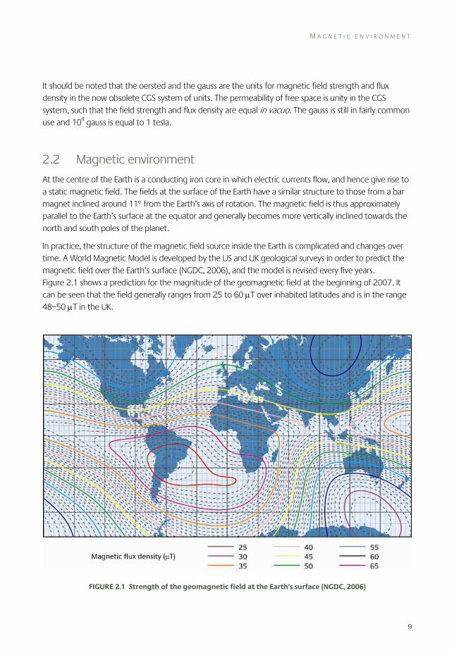
In practice, the structure of the magnetic field source inside the Earth is complicated and changes over time. A World Magnetic Model is developed by the US and UK geological surveys in order to predict the magnetic field over the Earth’s surface (NGDC, 2006), and the model is revised every five years. Figure 2.1 shows a prediction for the magnitude of the geomagnetic field at the beginning of 2007. It can be seen that the field generally ranges from 25 to 60 μT over inhabited latitudes and is in the range 48–50 μT in the UK.
FIGURE 2.1 Strength of the geomagnetic field at the Earth’s surface (NGDC, 2006)
2 S O U R C E S , E X P O S U R E S A N D M E A S U R E M E N T S
10
There is a slow variation of the geomagnetic field over time, known as the secular variation, and this is accounted for in the World Magnetic Model. In the UK, this variation is presently giving an increase in flux density of around 30 nT per year. There is also a diurnal variation in the magnetic field due to rotation of the Earth in the solar wind.
The geomagnetic field is affected by the solar wind, and variations in the sun’s output, eg due to geomagnetic storms, cause short-term changes in flux density and direction. These changes are usually small in relation to the overall magnitude of the geomagnetic field but can range up to a few microtesla during violent storms.
The magnetic field at the surface of the Earth can also vary from that shown in Figure 2.1 at some locations because of the presence of magnetic materials in rocks near the surface or nearby objects. Measurements that have been made in homes and workplaces are discussed in this section to illustrate the degree of perturbation of the geomagnetic field that can be expected at typical locations where people may be present.
2.2.1 Geomagnetic fields in homes
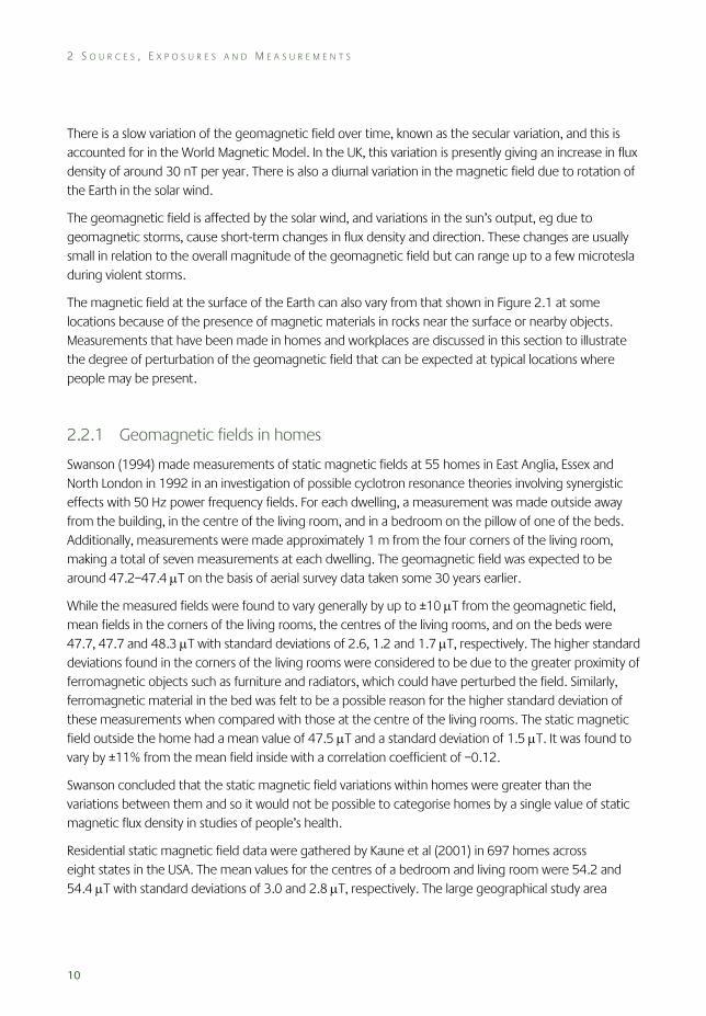
Swanson (1994) made measurements of static magnetic fields at 55 homes in East Anglia, Essex and North London in 1992 in an investigation of possible cyclotron resonance theories involving synergistic effects with 50 Hz power frequency fields. For each dwelling, a measurement was made outside away from the building, in the centre of the living room, and in a bedroom on the pillow of one of the beds. Additionally, measurements were made approximately 1 m from the four corners of the living room, making a total of seven measurements at each dwelling. The geomagnetic field was expected to be around 47.2–47.4 μT on the basis of aerial survey data taken some 30 years earlier.
While the measured fields were found to vary generally by up to ±10 μT from the geomagnetic field, mean fields in the corners of the living rooms, the centres of the living rooms, and on the beds were 47.7, 47.7 and 48.3 μT with standard deviations of 2.6, 1.2 and 1.7 μT, respectively. The higher standard deviations found in the corners of the living rooms were considered to be due to the greater proximity of ferromagnetic objects such as furniture and radiators, which could have perturbed the field. Similarly, ferromagnetic material in the bed was felt to be a possible reason for the higher standard deviation of these measurements when compared with those at the centre of the living rooms. The static magnetic field outside the home had a mean value of 47.5 μT and a standard deviation of 1.5 μT. It was found to vary by ±11% from the mean field inside with a correlation coefficient of –0.12.
Swanson concluded that the static magnetic field variations within homes were greater than the variations between them and so it would not be possible to categorise homes by a single value of static magnetic flux density in studies of people’s health.
Residential static magnetic field data were gathered by Kaune et al (2001) in 697 homes across eight states in the USA. The mean values for the centres of a bedroom and living room were 54.2 and 54.4 μT with standard deviations of 3.0 and 2.8 μT, respectively. The large geographical study area

M A G N E T I C E N V I R O N M E N T
11
meant that the geomagnetic field was expected to vary in the range 54–58 μT, and this explains why the standard deviations are higher than those found by Swanson.
The fields were systematically lower than the expected geomagnetic field across all states and all categories of dwellings. The majority of these (560) were classed as single family homes and the measured fields in the bedroom and living room were on average 2.5% and 2.7% lower than the geomagnetic field, respectively, both with standard errors of 0.2%. The reason for the attenuation of the geomagnetic field found inside homes by Kaune et al was unclear and the effect does not appear to be evident in the study by Swanson. Measurement errors were ruled out as a cause as the calibrations were regarded as accurate to ±1%.
Kaune et al also analysed temporal stability of residential static fields in a set of 51 homes in the Minneapolis St Paul and Detroit areas. Each home was visited seven times over a year, with around 61 days between the visits. Measurements were made at the centre of a living room and bedroom, and 5 cm above the bed. The coefficients of variation (standard deviation/mean) in the data for each measurement position were 1.4%, 7.4% and 1.2% with standard deviations of 1.3%, 8.2% and 0.7%, respectively. The measurement on the bed hence had poorer repeatability and this was regarded to be due to positioning errors having a larger effect in fields perturbed by ferromagnetic materials in the beds.
2.2.2 Geomagnetic fields in workplaces
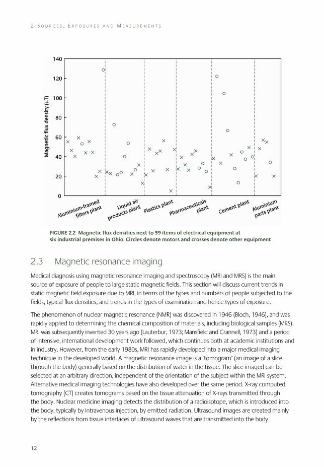
Bowman and Methner (2000) used a novel measuring instrument to capture magnetic field waveforms at six manufacturing premises in Ohio, USA. The premises were selected because they were heavy users of electricity since the processes involved were in the manufacture of plastics, pharmaceuticals, cement, liquid air products, aluminium parts and aluminium-framed filters. Measurements were made next to 59 items of electrical equipment at 1 m height at the locations where operators would be present.
The measurement instrument, known as the Multiwave II, was based on a three-axis fluxgate magnetometer having a bandwidth up to 3 kHz. The instrument was configured to acquire time-domain samples at a rate of 6142.5 Hz, as this would correspond to exactly five waveform cycles at the mains frequency of 60 Hz and the data were processed to identify the variation over time in the magnitude and direction of power frequency fields, and also the magnitude of the static field. The results are shown in Figure 2.2.
The field range was from 4.95 to 128.58 μT, with a median value of 39.24 μT. The geomagnetic field was stated to be 55 μT and the authors suggested that the median field was lower than this due to shielding of work locations by steel structures and machinery.
The five measurements over 60 μT were all next to equipment items described as motors by the authors, and the highest measurement was next to a 2 HP (1.5 kW) DC motor. Not all motors gave high static fields, possibly to some extent because not all of the field directions may have been such that they would have added to the geomagnetic field. Nevertheless, motors generally contain large amounts of ferromagnetic material and so it is not unexpected that they would perturb the geomagnetic field.
2 S O U R C E S , E X P O S U R E S A N D M E A S U R E M E N T S
12
FIGURE 2.2 Magnetic flux densities next to 59 items of electrical equipment at six industrial premises in Ohio. Circles denote motors and crosses denote other equipment
2.3 Magnetic resonance imaging
Medical diagnosis using magnetic resonance imaging and spectroscopy (MRI and MRS) is the main source of exposure of people to large static magnetic fields. This section will discuss current trends in static magnetic field exposure due to MRI, in terms of the types and numbers of people subjected to the fields, typical flux densities, and trends in the types of examination and hence types of exposure.
The phenomenon of nuclear magnetic resonance (NMR) was discovered in 1946 (Bloch, 1946), and was rapidly applied to determining the chemical composition of materials, including biological samples (MRS). MRI was subsequently invented 30 years ago (Lauterbur, 1973; Mansfield and Grannell, 1973) and a period of intensive, international development work followed, which continues both at academic institutions and in industry. However, from the early 1980s, MRI has rapidly developed into a major medical imaging technique in the developed world. A magnetic resonance image is a ‘tomogram’ (an image of a slice through the body) generally based on the distribution of water in the tissue. The slice imaged can be selected at an arbitrary direction, independent of the orientation of the subject within the MRI system. Alternative medical imaging technologies have also developed over the same period. X-ray computed tomography (CT) creates tomograms based on the tissue attenuation of X-rays transmitted through the body. Nuclear medicine imaging detects the distribution of a radioisotope, which is introduced into the body, typically by intravenous injection, by emitted radiation. Ultrasound images are created mainly by the reflections from tissue interfaces of ultrasound waves that are transmitted into the body.
M A G N E T I C R E S O N A N C E I M A G I N G
13
The enormous expansion in MRI during the last 30 years is due to the versatility of the technique. First, MRI is a global anatomical imaging modality; it can provide excellent, detailed images of soft tissue with a wide contrast range. In this it competes with X-ray computed tomography (CT) for whole body imaging coverage. The situations where MRI or CT is the modality of choice evolve as the two technologies continue to develop. However, some patients will never be suitable for MRI (since they have contraindications such as an implanted pacemaker), but CT gives a high dose of ionising radiation to patients (Paterson and Frush, 2007). The lack of exposure to ionising radiation means that MRI has particular advantages over CT in paediatric radiology (where the radiation dose is critical) and abdominal imaging (where the radiation dose is often very high). Most imaging techniques rely upon one or two contrast mechanisms – for instance, based on the differences in tissue density and atomic number (X-ray techniques), or acoustic impedance and motion of tissue (ultrasound). However, the MRI signal can be modulated to generate contrast based on a wide range of parameters related to water binding, the concentration of macromolecules in the tissue, the concentration of iron containing molecules in the tissue, and others.
Second, MRI is a functional imaging modality, similar to nuclear medicine techniques. For instance, it can be used to measure blood flow in vessels, tissue perfusion or changes in blood oxygenation. Using MRS, it is even possible to study metabolism in vivo.
Third, MRI is a dynamic imaging modality and images can be acquired continuously in a similar fashion to ultrasound. For instance, MRI can be used to study the movement of joints, or the handling of a meal in the gastrointestinal tract.
The versatility and flexibility of MRI, its apparent relative safety and non-invasive nature, have led to an enormous increase in demand for examinations over the last two decades. This chapter will explain how MRI works, the extent and degree of exposures, and the major drivers in the field at present that are likely to lead to an increase in exposure over the next decade.
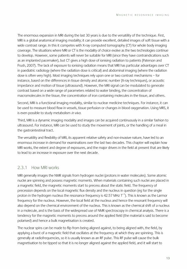
2.3.1 How MRI works
MRI generally images the NMR signals from hydrogen nuclei (protons in water molecules). Some atomic nuclei are spinning and possess magnetic moments. When materials containing such nuclei are placed in a magnetic field, the magnetic moments start to precess about the static field. The frequency of precession depends on the local magnetic flux density and the nucleus in question (eg for the single proton in the hydrogen nucleus the resonance frequency is 42.57 MHz T−1). This is known as the Larmor frequency for the nucleus. However, the local field at the nucleus and hence the resonant frequency will also depend on the chemical environment of the nucleus. This is known as the chemical shift of a nucleus in a molecule, and is the basis of the widespread use of NMR spectroscopy in chemical analysis. There is a tendency for the magnetic moments to precess around the applied field (the material is said to become polarised) and hence a bulk magnetisation is created.
The nuclear spins can be made to flip from being aligned against, to being aligned with, the field, by applying a burst of a magnetic field that oscillates at the frequency at which they are spinning. This is generally at radiofrequencies, so it is usually known as an RF pulse. This RF pulse will cause the bulk magnetisation to be tipped so that it is no longer aligned against the applied field, and it will start to

2 S O U R C E S , E X P O S U R E S A N D M E A S U R E M E N T S
14
rotate about the applied field, also at the same Larmor frequency. The rotating bulk magnetisation will induce a voltage at the Larmor frequency in a pick-up coil placed close to the sample, and this is the NMR signal that is detected. To form an image, the static field is made to vary linearly through space (a magnetic field gradient). This means that the Larmor frequency of the NMR signal now codes for spatial position. This magnetic field gradient is switched on and off very rapidly during imaging sequences.
From this explanation, it can be seen that three types of magnetic fields are used in MRI. These are the static field (around 1 T), the gradient fields (around 20 mT m–1 varied with a period of around 1 ms, but with a highly complex waveform), and the RF fields (around 10 μT). The static field effectively exposes staff and patients to a large static field, a spatial gradient of field (as it falls off around the magnet) and a small time-varying field (if an individual moves around in the spatially varying, static field). The static field is usually created by a superconducting magnet, which it is not practical to switch on and off rapidly. However, the gradient field is switched on and off very rapidly during an examination and so exposes patients to large time-varying fields, although in general staff are less frequently exposed to this. Similarly, the RF field exposes patients to magnetic fields that are varying extremely rapidly. This chapter generally considers only the effect of static magnetic fields, although it should be noted that as both patients and staff must physically move through the static field as part of the MRI examination they are also inevitably exposed to time-varying magnetic fields.
2.3.2 Numbers of people exposed
The increasing take up of MRI, and the expansion of MRI into new areas of application, is demonstrated by the growth in the number of scanners in the UK from about 10 in 1991 to about 400 today (de Wilde, 2004). An unpublished survey carried out on behalf of the Institute of Physics and Engineering in Medicine (Moore et al, 2006) found 438 National Health Service and private systems in the UK at 326 hospitals/clinics; this excludes about 20 scanners situated in university departments. Based on the responses to the survey an estimated 1.37 million clinical MRI examinations are carried out each year in the whole of the UK, corresponding to 2.5% of the population having an MRI scan each year. This figure is set to increase as the NHS (the main provider of medical care in the UK) is currently purchasing more MRI capacity. It seems likely that this trend will continue for some time because some applications of MRI are currently limited only because of cost, and as MRI scanner numbers have increased they have become cheaper, and hence feasible areas of application increase. In some instances, such as breast screening, this may lead to the construction of cheaper, dedicated niche MRI systems, further increasing utilisation.
Another recent trend has been an increase in the number of MRI systems that are dedicated to research, and which are owned and operated by non-clinical university departments. There are probably about 20 of these systems in the UK and they are used predominantly to examine healthy volunteers rather than patients and they may be operated by technical staff rather than by clinically trained radiographers. Research scanners are most frequently used in neuroscience, although they are also increasingly used in the pharmaceutical industry.
M A G N E T I C R E S O N A N C E I M A G I N G
15
2.3.3 Exposure levels
Currently the most widely used magnetic flux density for clinical MRI is 1.5 T. However, the optimum flux density for many applications continues to be debated, and tends to evolve upwards as the technical difficulties facing some applications in strong fields are overcome. For the first decade of MRI, there was no clear preference for fields between 0.5 and 1.5 T, but in the last decade, 1.5 T has become the primary flux density for routine clinical scanning, and there are now probably fewer than 20 standard MRI scanners operating at 1.0 T or less in the UK. Magnets operating at 3 T appeared in the early 1990s and until recently their use has been restricted to research laboratories. However, they are rapidly becoming the magnets of choice in centres dedicated to neuroimaging, and it was estimated that there were 35 in the UK in 2007. Niche application and interventional scanners have tended to use weaker magnets (0.5 T or less), but even for these uses there has been a trend toward higher fields (manufacturers are currently marketing 1.0 T open systems). More recently ultrahigh field magnets have started to receive more attention, the first 8 T whole body magnet becoming operational in 1998. Scanners operating at 7 T have been installed at a few research sites, and there is currently estimated to be a worldwide market for about ten to fifteen 7 T scanners, although this will undoubtedly increase over the next five years. The first 9.4 T whole body magnet was delivered in 2003 and an 11.7 T whole body scanner is to be installed in Paris in the near future.
Broadly speaking, as the magnetic flux density increases, the signal to noise ratio in an image increases approximately linearly. This is because the signal increases quadratically (because it depends on both the polarisation of the tissue and induction), whereas the noise only increases linearly (as it depends only on induction). Therefore if the magnetic flux density is doubled, the signal to noise ratio will be doubled. This improved signal to noise ratio can be used in a variety of ways. Most commonly, the increased signal is used to reduce the size of the image pixels, and hence increase the spatial resolution. This allows detection of previously hidden anatomical detail, and high field MRI is now providing images with a detail that can otherwise generally only be obtained from pathology. The increased signal can also be used to reduce the amount of signal averaging, which allows reduction in the total examination time. This will potentially increase patient throughput, but is also useful clinically for uncooperative patients such as children, or acutely sick patients. Related to this, the shorter imaging times can be used to reduce the length of the data acquisition. This can reduce image artefacts related to inhomogeneities in the static magnetic field. Finally, the shorter imaging times can be used to carry out dynamic studies of systems that are changing. For instance, dynamic MRI is widely used to study the time course of uptake of a contrast agent in an organ such as the liver which may help both detect and characterise tumours.
Another effect of increasing the magnetic flux density is that NMR relaxation times increase, so after an RF pulse it takes longer for the magnetisation to return to its original value. This can be a disadvantage, as it tends to make examination times longer. However, it does provide an advantage in pulse sequences using MRI to measure blood flow or tissue perfusion. This makes it possible to study the blood vessels of the head in much more detail, which is important, for instance, when investigating conditions that can lead to stroke.
2 S O U R C E S , E X P O S U R E S A N D M E A S U R E M E N T S
16
An alternative method of studying blood flow involves injecting a contrast agent. These are chemicals that change the NMR relaxation times of the blood or tissue, and are often used to enhance the signal from tumours. There are a few side effects associated with them, and clearly it is preferable to minimise the dose used; at 3 T, enhancement of the image contrast can be obtained using less contrast agent than at 1.5 T (Krautmacher et al, 2005).
Increasing the magnetic field also creates new difficulties. First, if there are considerable variations in the magnetic susceptibility of the tissue, eg air in the nasal sinuses, then the local field is altered by an amount that is proportional to the applied field. This will combine with the effect of the applied magnetic gradient fields, and confuse the image encoding, leading to both geometric distortion and signal loss. These susceptibility artefacts get worse in routine clinical imaging as the field is increased, and this is a major technical hurdle to be overcome for stronger fields. However, there is also a diagnostically useful difference between the magnetic susceptibility of deoxygenated blood and oxygenated blood or tissue. The resulting microscopic changes in susceptibility around blood vessels are the basis of the blood oxygenation level dependent (BOLD) effect that is used to map brain activation in response to a stimulus or during a task. The sensitivity of the BOLD effect increases in stronger fields, and this is one of the main drivers towards stronger fields in neuroscience research MRI systems.
Second, at higher static magnetic flux densities, more RF energy is required to produce an image and the increase is approximately as the square of the flux density. RF energy deposited in tissue causes heating of the tissue, and therefore at higher flux densities, fewer RF pulses can be applied before the limits on power deposition are exceeded. This limits some applications of MRI at high flux densities, particularly where the whole body (rather than just the head) is exposed to the RF heating effect. Furthermore at high flux densities, the distribution of RF energy across the organs becomes less homogeneous, which leads to large variations in both RF energy deposition and resulting image intensity.
Finally, the chemical shift between different molecular species increases in stronger magnetic fields. This is an advantage for spectroscopy as it increases the resolution of the NMR spectra and the feasibility of performing NMR spectroscopy in vivo (MRS). However, it does have a disadvantage for imaging as a chemical shift artefact arises from the spatial location image of fat being shifted a few pixels with respect to the location of the protons in water. This effect is worse at higher flux densities and the solution (increasing receiver bandwidth) has the undesirable effect of reducing the signal to noise ratio.
At present, the major limit to increasing the magnetic field in MRI systems is the cost and local structural constraints of installing a high field magnet. However, during the last three decades, the relative cost of the magnets has decreased and magnet shielding technology has advanced making it simpler to install a magnet within existing buildings. Active shielding reduces the stray field outside the magnet bore and therefore the field experienced by the staff working around the magnet. However, as the shielding becomes more effective, so the gradient of the magnetic field away from the bore is increased. The main established hazard of MRI is the so-called ‘projectile effect’. This term is used to describe the force on, and hence acceleration of, any ferromagnetic object in the vicinity of the magnet. A person can be killed if they are hit by an object that is accelerated in this way. This force is proportional to the product of the static magnetic flux density and its gradient (B dB/dz), and therefore this hazard is increased in the vicinity of a shielded magnet compared with an unshielded one.
M A G N E T I C R E S O N A N C E I M A G I N G
17
2.3.4 New areas of application
Until recently clinical MRI scans have generally been performed within hospital radiology departments, but it is possible that this may change. Interventional MRI is now being used to monitor therapeutic procedures, and niche MRI systems are beginning to appear outside radiology departments. It is important to ensure that these MRI systems, in common with more standard installations, are subject to strict safety management. However, they also have implications for exposure to static magnetic fields. In particular, as discussed above, interventional MRI will increase the exposure of staff to static magnetic fields, as well as magnetic field gradients and RF fields.
Interventional radiology generally involves medical imaging techniques to guide a therapeutic or diagnostic procedure. These procedures traditionally use X-ray guidance and are associated with a high ionising radiation dose to patients (fluoroscopy accounts for 6% of medical imaging procedures but 27% of the dose) (ICRP, 2001) and a radiation dose to staff (Haskal, 2004). Interventional MRI is a new field of work, and is complicated by the need for all equipment, such as catheters, surgical instruments and monitoring equipment, to be MRI compatible. Despite the technical challenges of developing adequate MRI fluoroscopic techniques, this application of MRI is developing quickly. MRI has been used to guide tumour resection in real time and this has led to a reduced rate of tumour recurrence and hence repeat resection (Hall et al, 2000, 2005; Martin et al, 2000). The use of intraoperative MRI has also led to a reduced complication rate, because the procedure required smaller craniotomies and because post-operative haemorrhage could be detected rapidly on an MRI scan. This has led to a reduction in the length of hospital stay, and a reduction in the cost of the total procedure, even taking into account the cost of the intraoperative MRI (Hall et al, 2001; Kucharczyk et al, 2001).
Interventional MRI has also been used to guide cardiac catheterisation and electrophysiology studies (Martin et al, 2002; Razavi et al, 2003); in special combined units, patients can be transferred between an X-ray catheterisation laboratory and an interventional MRI scanner on a floating table. The three-dimensional anatomical and functional imaging capabilities, including improved soft tissue contrast, of MRI compared with X-ray techniques, allows some important functional parameters to be measured during scanning. Normally, paediatric cardiac patients often undergo multiple, complex and lengthy, X-ray guided, cardiovascular interventions, exposing them to an effective dose of around 6 mSv. The projected lifetime risk of fatal cancer due to this dose is estimated as 0.1–0.05% (decreasing with age at exposure during childhood) (Bacher et al, 2005), and thus the risk of radiation-induced cancer is estimated to be increased for this group of patients. Using interventional MRI in the future it is expected that the X-ray dose will be greatly reduced or even totally eliminated. If both MRI and X-ray procedures are required, then by combining the MRI and X-ray procedures in one laboratory on one occasion, only one anaesthetic, one catheterisation and one attendance at hospital is required, instead of two or more.
A combined MRI/catheterisation laboratory has also been used to guide chemotherapy (Martin et al, 2002) using a chemotherapy agent that has been tagged to be MRI visible. Initially, a baseline MRI scan is performed, and the patient is then transferred via a floating tabletop to the catheterisation laboratory, where a feeding vessel to the organ of interest is selected and the agent is delivered. The patient is then
2 S O U R C E S , E X P O S U R E S A N D M E A S U R E M E N T S
18
returned to the MRI scanner, to determine the drug distribution (indicated by the change in signal intensity caused by the chemotherapy agent). Based on the MRI information, the catheter can then be repositioned and a second injection can be delivered. This process can be repeated until adequate coverage of the tumour has been achieved or the toxic limit of the drug is reached.
Small, dedicated MRI scanners are being sited outside radiology departments; a common example is the use of small bore MRI systems for orthopaedic imaging. Similar scanners are also being used for imaging neonates within the neonatal unit, to avoid the risks associated with transferring them to the radiology department.
Finally, it should be noted that as well as examining people in hospitals and research institutions, MRI is also used to scan animals and samples such as rock cores in research institutions. MRI is increasingly being used in the pharmaceutical industry, where it has the potential to reduce greatly the number of animals used to test drugs, as imaging allows the time course of the effects of the drugs to be studied. These magnets often have stronger fields (around 7 T) than the clinical scanners, but they have a smaller bore (around 30 cm), making it harder for the staff to expose more than their arms to regions of high field strength. Vertical bore magnets are also in use in research institutions for microscopic imaging and chemical analysis. They can typically operate at fields of 12 T, but in these magnets it is usually impossible for staff to access regions where such fields are present. Various designs of MRI scanners are also being used in veterinary medicine.
2.3.5 Classes of staff exposed
As well as exposures to the patient, MRI examinations expose radiography and medical staff, service engineers and research volunteers to static magnetic fields. There are few detailed exposure data available at present for the different classes of staff discussed above, and the collection of such data is hampered by the lack of a suitable personal dosemeter. Since all these groups must inevitably move within the static field, they are also exposed to slowly time-varying fields (around <10 Hz) creating rates of change of field, dB/dt, of up to 2 T s–1 (Cavin et al, 2007). However, radiography and medical staff are not routinely exposed to the RF field or the time-varying gradient fields; this occurs only if they are required to stand near the end of the bore during an examination (eg reassuring a child or during an interventional MRI procedure) (at levels of around 50 μT at 40 cm from the end of the bore [Riches et al, 2007]).
Radiographers form the largest group of workers who are occupationally exposed to static magnetic fields. Their role is to look after patients’ comfort and safety, and to operate the MRI system efficiently. Radiographers intermittently walk through the static field around the magnet throughout their working day, and hence they probably receive the greatest exposure (up to around 0.1 T to the whole body). When a patient is positioned the radiographer often has to reach into the bore to ensure that the patient is comfortable and that any monitoring equipment (such as electrocardiogram (ECG) leads and respiratory monitoring cables) is safely and correctly positioned. Distressed and seriously ill patients often require closer monitoring and the radiographer may need to lean into the bore of the magnet to
M A G N E T I C R E S O N A N C E I M A G I N G
19
reassure the patient during the examination, which will increase their exposure (up to around 2 T, the approximate field at the end of most magnets with central fields of 1.5 T (shielded) to 7 T, to the head, arms and upper torso). In some research sites, clinically qualified radiographers are replaced by staff with no formal qualifications related to magnetic resonance. There is little published information on the exposures of staff to static fields. The limited data available indicate time-averaged exposures of approximately 14±10 mT over 24 hours for radiographers working around 1.5 T scanners (Bradley, 2005), with similar values reported for MRI technicians working around 3 T scanners (Cavin et al, 2007). However, there is considerable variation in the integrated exposure of different members of staff undertaking the same task (Cavin et al, 2007), and the results are likely to be extremely dependent on the design of magnet and on the work being undertaken.
The medical staff who are clinically responsible for MRI scans (radiologists) are less involved in direct patient care but nevertheless may be exposed to the static field in the same way as radiographers, particularly to administer any contrast agents (drugs that change the signal in the image) required during the procedure or to supervise an ill patient. The expansion of interventional MRI will greatly increase the exposure of radiologists to magnetic fields including the gradient and RF fields, as they will have to be in close contact with the patient during scanning. Other medical staff such as anaesthetists are sometimes involved in scanning sick or uncooperative patients and they may also be close to the patients during scanning, although they may also be able to operate from outside the MRI room where possible.
Another group of staff exposed to static fields are the engineers involved in constructing the MRI scanners and maintaining them on site. Careful working practices can minimise exposure from routine work but if a component breaks down within the scanner, they may have to climb inside to remove it. Field engineers typically spend a large proportion of their working day inside the MRI rooms, although there are few published exposure data for this group.
The physicists, engineers and developmental staff (who may include both radiography and medical staff) in industry, universities and hospitals – whose role is to develop and optimise the capabilities of MRI – can receive considerable exposure. These groups of staff will often use novel scanners or use standard scanners in non-standard ways, which frequently involves them climbing inside the magnet to adjust new pieces of hardware, and thus being exposed to strong magnetic fields. Testing of new imaging examinations and the optimisation of MRI examinations are frequently performed using these staff as volunteers, prior to their use on patients. This process of protocol optimisation on volunteers is very widely performed on clinical MRI systems, even those not directly involved in research.
It is important to note that as well as scanning patients, healthy volunteers are also frequently scanned, under ethics committee approval. This can be to answer questions about normal human physiological and psychological function. However, due to the sensitivity of MRI to the function of living biological tissue (blood flow, movement, etc), normal volunteers are also scanned in developing and optimising new imaging techniques, because test phantoms cannot be created to mimic living tissue adequately. It is worth noting that some individuals (particularly MRI workers) may be scanned as volunteers many times.
2 S O U R C E S , E X P O S U R E S A N D M E A S U R E M E N T S
20
2.4 Other static magnetic field sources
Electrical equipment can produce magnetic fields either as a deliberate part or as a byproduct of its normal operation. Direct current (DC) flows are required to produce static fields; however, such currents are frequently derived in practice from the rectification of alternating currents (AC) at 50/60 Hz. Where there is imperfect smoothing of the rectified currents, the magnetic fields contain components at 50/60 Hz and its harmonics as well as a static components. Permanent magnets give rise to pure static magnetic fields.
The context for artificially generated magnetic fields is that all people are continuously exposed to the geomagnetic field of 48–50 μT (in the UK). Artificially generated fields add to (or subtract from) this field according to the relative vector orientations. Sometimes experimental equipment is used deliberately to cancel out the geomagnetic field at a particular location so that processes that are sensitive to magnetic fields can be carried out in isolation.
Stuchly (1986) reviewed human exposure to static magnetic fields in a paper drawing on a range of information sources including conference papers, dissertations and technical reports, as well as peer-reviewed information from journals. Other more recent reviews of the topic are in Allen et al (1994), Cooper (2002) and WHO (2006). Original sources of information dating from the mid-1970s are included in the Stuchly review; however, few original papers seem to have been published since. This section summarises the published information regarding the static magnetic fields produced by a range of sources and the relevant exposure conditions for people in the vicinity of the sources. It also draws on unpublished data from surveys performed by the HPA, where little information is available from other sources.
Many reported measurements aim to investigate compliance with exposure guidelines, eg as published by ICNIRP (www.icnirp.org), and tend to represent maximum exposure levels that can occur at normally accessible locations. For other purposes, eg health research studies, there may be an interest in more typical exposure values, or the range of exposure values that occurs during normal work activities. Such information is not so readily available in the literature.
2.4.1 Electrochemical industry
Various industries use electrolysis to extract chemicals from conducting liquids and the large currents involved give rise to static magnetic fields. Pairs of electrodes are inserted into a cell containing the liquid and a current is passed between them, resulting in either anions or cations in the liquid being converted into uncharged chemicals at the electrodes.
A solution of sodium chloride is electrolysed in the chloralkali industry and hydrogen gas is collected at the cathode and chlorine gas is collected at the anode. An alkaline solution of sodium hydroxide (caustic soda) is the residue of the process.
In the aluminium industry, molten ore, known as alumina is electrolysed. Oxygen gas is produced at the anode and molten aluminium metal is formed at the cathode, where it sinks to the bottom of the cell and is tapped-off.

O T H E R S T A T I C M A G N E T I C F I E L D S O U R C E S
21
Many, perhaps hundreds, of electrolysis cells can be located near to each other in a manufacturing plant, with power supply bus-bars passing the length of the production area with taps carrying the currents to individual cells. Potential differences between the bus-bars are a few hundred volts, but the currents are many thousands of amperes so strong magnetic fields are generated. In order to minimise resistive losses and heating, the bus-bars are substantial multi-vaned conductors of large cross-sectional area, as shown in Figure 2.3.
FIGURE 2.3 Power supply bus-bars in the roof of a corridor at a chloralkali plant (courtesy of Ineos Chlor)
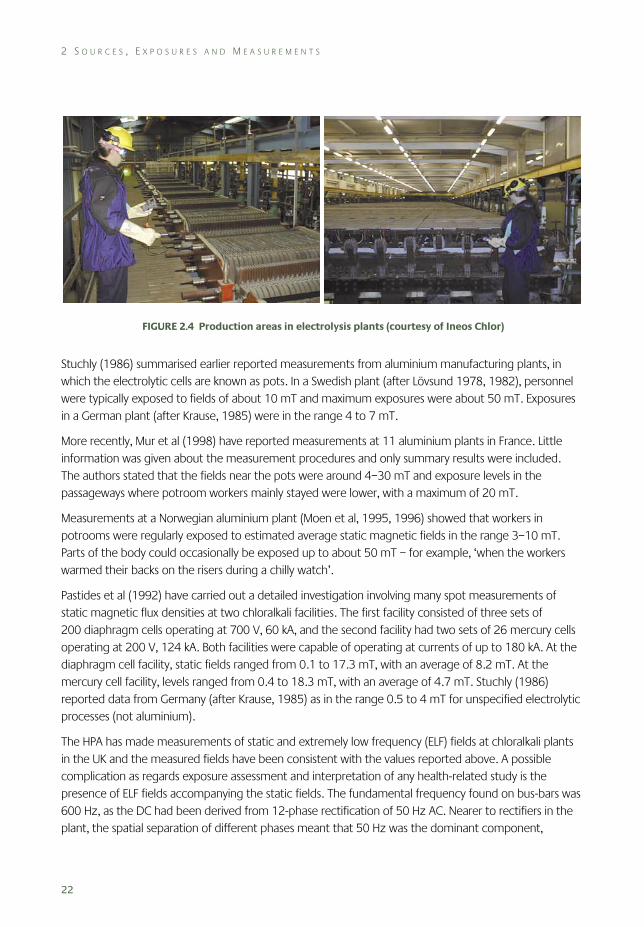
Exposures to static magnetic fields occur when people are in the vicinity of the cells and bus-bars, and some staff may be present at these locations for many hours each day. Typical production areas with arrays of electrolysis cells are shown in Figure 2.4. It is estimated that there are around 150 electrolysis plants in Europe.
Marsh et al (1982) carried out a cross-sectional study involving 320 workers who spent a large portion of their working day near electrolysis cells containing either sodium or magnesium chloride solution. Data from time and motion studies were available for the workers allowing spot measurements of magnetic field to be weighted and combined in order to evaluate time-averaged exposures. The authors noted that variations in the orientation of the fields with respect to the body may have been an important consideration in developing exposure metrics and that the orientation with respect to the horizontal field component would be more variable than that to the vertical component. A range of descriptive statistics was given, including that the mean static magnetic field level at operator positions was 7.6 mT and the maximum was 14.6 mT. Time-weighted-average field exposures were calculated to be about 5 and 13.7 mT for the mean and maximum field levels, respectively.
2 S O U R C E S , E X P O S U R E S A N D M E A S U R E M E N T S
22
FIGURE 2.4 Production areas in electrolysis plants (courtesy of Ineos Chlor)
Stuchly (1986) summarised earlier reported measurements from aluminium manufacturing plants, in which the electrolytic cells are known as pots. In a Swedish plant (after Lövsund 1978, 1982), personnel were typically exposed to fields of about 10 mT and maximum exposures were about 50 mT. Exposures in a German plant (after Krause, 1985) were in the range 4 to 7 mT.
More recently, Mur et al (1998) have reported measurements at 11 aluminium plants in France. Little information was given about the measurement procedures and only summary results were included. The authors stated that the fields near the pots were around 4–30 mT and exposure levels in the passageways where potroom workers mainly stayed were lower, with a maximum of 20 mT.
Measurements at a Norwegian aluminium plant (Moen et al, 1995, 1996) showed that workers in potrooms were regularly exposed to estimated average static magnetic fields in the range 3–10 mT. Parts of the body could occasionally be exposed up to about 50 mT – for example, ‘when the workers warmed their backs on the risers during a chilly watch’.
Pastides et al (1992) have carried out a detailed investigation involving many spot measurements of static magnetic flux densities at two chloralkali facilities. The first facility consisted of three sets of 200 diaphragm cells operating at 700 V, 60 kA, and the second facility had two sets of 26 mercury cells operating at 200 V, 124 kA. Both facilities were capable of operating at currents of up to 180 kA. At the diaphragm cell facility, static fields ranged from 0.1 to 17.3 mT, with an average of 8.2 mT. At the mercury cell facility, levels ranged from 0.4 to 18.3 mT, with an average of 4.7 mT. Stuchly (1986) reported data from Germany (after Krause, 1985) as in the range 0.5 to 4 mT for unspecified electrolytic processes (not aluminium).
The HPA has made measurements of static and extremely low frequency (ELF) fields at chloralkali plants in the UK and the measured fields have been consistent with the values reported above. A possible complication as regards exposure assessment and interpretation of any health-related study is the presence of ELF fields accompanying the static fields. The fundamental frequency found on bus-bars was 600 Hz, as the DC had been derived from 12-phase rectification of 50 Hz AC. Nearer to rectifiers in the plant, the spatial separation of different phases meant that 50 Hz was the dominant component,
O T H E R S T A T I C M A G N E T I C F I E L D S O U R C E S
23
together with harmonics. In both cases, frequency components extending up to several kilohertz were found in the measurements.
2.4.2 Transport systems
Many different types of electrically powered transport systems exist and wherever DC supplies are used static magnetic fields will be present. Some traction motors use DC, although often the currents will be switched on and off rapidly (chopped) with a variable duty factor in order to control the total power consumption. This introduces time-varying magnetic fields, typically with frequencies of the order of a kilohertz.
Dietrich and Jacobs (1999) prepared a substantial technical report on public exposure to static and ELF time-varying electric and magnetic fields in transport systems under the US Department of Energy EMF Research and Public Information Dissemination (EMF-RAPID) Engineering Research Program. The work was carried out on systems in the North Eastern USA, mostly in the New York area, where the static magnetic flux density was around 54 μT in 1999. Measurements were made using a triaxial fluxgate magnetometer to acquire sampled waveforms and Table 2.1 summarises the results. Generally, the data were gathered at three heights at each measurement position, eg 30, 90 and 150 cm above floor level, but only the data for 90 cm or waist height have been included in Table 2.1
For most of the sources in Table 2.1, the static fields measured were concluded to be geomagnetic fields perturbed by, and with varying degrees of shielding from, the structure of the transport system being investigated. For some of the sources, the data gathered over height showed greater shielding of the geomagnetic field at lower heights, eg escalators and moving walkways, where the measurement would have been in closer proximity to steelwork. There was some suggestion in the data that static magnetic fields were produced at some ankle-level locations in the electric cars, trucks and buses, and also in the commuter train, all of which used DC supplies. However, any artificially generated static fields were felt neither to add appreciably to nor to alter the extent of variability within the total static field environment inside the vehicles.
The technical aspects of electric railways in the UK, together with some measurements of exposure, have been summarised by Chadwick and Lowes (1998). The systems fall into two broad categories: those that use a 25 kV AC overhead supply and those that use around 600–700 V DC supplied to the train via one or more extra rails. Both categories tended to use DC traction motors, with AC-fed trains having on-board voltage down-conversion and rectification. However, a trend was noted for newer trains to move to AC traction motors with the frequency of the AC varied in proportion to the motor speed.
Chadwick and Lowes cautioned that their measurements were based on a small number of reported observations and were not necessarily typical. For a London Underground train, static magnetic flux densities at floor level were in the range 0.1–2 mT inside the passenger compartment of a motorised car and 0.2 mT in the driver’s cab, while all measurements were below 0.2 mT at a height of 1 m. For a suburban train, the magnetic flux densities at table height inside the passenger compartment were in the range 16–64 μT, while they were up to 1 mT at floor level.
2 S O U R C E S , E X P O S U R E S A N D M E A S U R E M E N T S
24
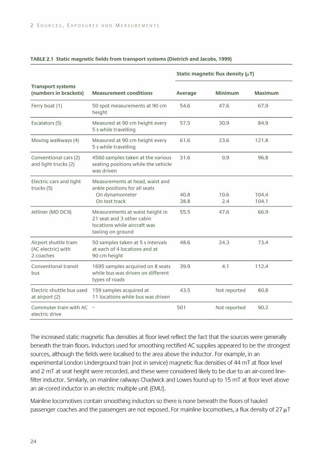
TABLE 2.1 Static magnetic fields from transport systems (Dietrich and Jacobs, 1999)
Static magnetic flux density (μT)
Transport systems (numbers in brackets) Measurement conditions Average Minimum Maximum
Ferry boat (1) 50 spot measurements at 90 cm height
54.6 47.6 67.9
Escalators (5) Measured at 90 cm height every 5 s while travelling
57.5 30.9 84.9
Moving walkways (4) Measured at 90 cm height every 5 s while travelling
61.6 23.6 121.8
Conventional cars (2) and light trucks (2)
4560 samples taken at the various seating positions while the vehicle was driven
31.6 0.9 96.8
Electric cars and light trucks (5)
Measurements at head, waist and ankle positions for all seats On dynamometer On test track
40.8 38.8
10.6 2.4
104.4 104.1
Jetliner (MD DC9) Measurements at waist height in 21 seat and 3 other cabin locations while aircraft was taxiing on ground
55.5 47.6 66.9
Airport shuttle tram (AC electric) with 2 coaches
50 samples taken at 5 s intervals at each of 4 locations and at 90 cm height
48.6 24.3 73.4
Conventional transit bus
1695 samples acquired on 8 seats while bus was driven on different types of roads
39.9 4.1 112.4
Electric shuttle bus used at airport (2)
159 samples acquired at 11 locations while bus was driven
43.5 Not reported 80.8
Commuter train with AC electric drive
– 501 Not reported 90.2
The increased static magnetic flux densities at floor level reflect the fact that the sources were generally beneath the train floors. Inductors used for smoothing rectified AC supplies appeared to be the strongest sources, although the fields were localised to the area above the inductor. For example, in an experimental London Underground train (not in service) magnetic flux densities of 44 mT at floor level and 2 mT at seat height were recorded, and these were considered likely to be due to an air-cored line-filter inductor. Similarly, on mainline railways Chadwick and Lowes found up to 15 mT at floor level above an air-cored inductor in an electric multiple unit (EMU).
Mainline locomotives contain smoothing inductors so there is none beneath the floors of hauled passenger coaches and the passengers are not exposed. For mainline locomotives, a flux density of 27 μT
O T H E R S T A T I C M A G N E T I C F I E L D S O U R C E S
25
was found 1.4 m above the floor of the driver’s cab and up to 3 mT was found 0.5 m above the floor in the equipment car.
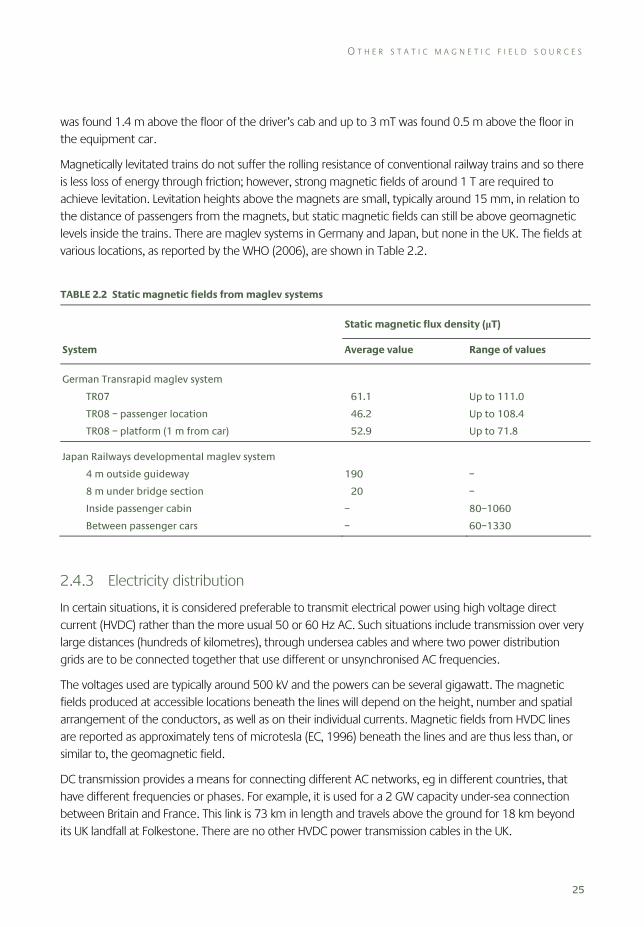
Magnetically levitated trains do not suffer the rolling resistance of conventional railway trains and so there is less loss of energy through friction; however, strong magnetic fields of around 1 T are required to achieve levitation. Levitation heights above the magnets are small, typically around 15 mm, in relation to the distance of passengers from the magnets, but static magnetic fields can still be above geomagnetic levels inside the trains. There are maglev systems in Germany and Japan, but none in the UK. The fields at various locations, as reported by the WHO (2006), are shown in Table 2.2.
TABLE 2.2 Static magnetic fields from maglev systems
Static magnetic flux density (μT)
System Average value Range of values
German Transrapid maglev system
TR07
TR08 – passenger location
TR08 – platform (1 m from car)
61.1
46.2
52.9
Up to 111.0
Up to 108.4
Up to 71.8
Japan Railways developmental maglev system
4 m outside guideway
8 m under bridge section
Inside passenger cabin
Between passenger cars
190
20
–
–
–
–
80–1060
60–1330
2.4.3 Electricity distribution
In certain situations, it is considered preferable to transmit electrical power using high voltage direct current (HVDC) rather than the more usual 50 or 60 Hz AC. Such situations include transmission over very large distances (hundreds of kilometres), through undersea cables and where two power distribution grids are to be connected together that use different or unsynchronised AC frequencies.
The voltages used are typically around 500 kV and the powers can be several gigawatt. The magnetic fields produced at accessible locations beneath the lines will depend on the height, number and spatial arrangement of the conductors, as well as on their individual currents. Magnetic fields from HVDC lines are reported as approximately tens of microtesla (EC, 1996) beneath the lines and are thus less than, or similar to, the geomagnetic field.
DC transmission provides a means for connecting different AC networks, eg in different countries, that have different frequencies or phases. For example, it is used for a 2 GW capacity under-sea connection between Britain and France. This link is 73 km in length and travels above the ground for 18 km beyond its UK landfall at Folkestone. There are no other HVDC power transmission cables in the UK.
2 S O U R C E S , E X P O S U R E S A N D M E A S U R E M E N T S
26
2.4.4 Welding
An overview of the different arc welding and resistance welding technologies, together with a literature review of exposure assessment studies, is given by Melton (2005). Most of the studies in the literature are concerned with time-varying fields and only those few that report static fields are mentioned here.
The equipment can use DC or AC supplies depending on the application and static magnetic fields arise where DC is used. However, the DC supplies are derived from rectification of 50 Hz AC and therefore carry harmonics of 100 Hz in the case of single phase rectification and higher frequencies in the case of three or more phase rectification. With some systems the DC supplies are pulsed through chopping the waveform and this can be at frequencies of several hundred hertz.
Typical welding currents used with MMA (metal-metal arc) and MIG/MAG (metal inert/active gas) welders range up to around 600 A. Resistance welding involves contact between two electrodes and the material being welded and generally uses higher currents than arc welding, up to around 10 kA for continuous currents and still higher with pulsed currents.
Exposure of the operator occurs due to their proximity to the current-carrying conductors feeding the electrodes, which in the case of manually operated welding equipment may be draped across the body or over the shoulders. In this situation, the magnetic field is inversely proportional to the distance and so the body is exposed non-uniformly. The cables of automatically operated equipment are usually not so close to the operator and exposures would be expected to be lower.
Skotte and Hjøllund (1997) made magnetic field exposure measurements for a cohort of Danish welding workers. The main interest of the investigation was ELF fields but some measurements of static fields from DC welders were made with a Hall effect sensor. All of the measurements were made at 1 cm from the welder cables. A 5 mT field was measured for a submerged arc welder (used under water) and the fields from MIG/MAG welders were in the range 0.9–1.9 mT.
Cooper (2002) included measurements of static magnetic fields from resistance welders in a technical report reviewing occupational exposure to various sources. For a 250 kVA DC welder delivering a current of 14.1 kA, the field was 30 mT at 5 cm from the electrodes and 10 mT at 20 cm. A DC welder delivering a current of 8 kA derived from rectification of an 800 Hz supply produced 1 mT where the limbs of the operator could be exposed and 0.2 mT where the body of the operator would typically be situated.
2.4.5 Scientific applications
Nuclear magnetic resonance is used in a variety of spectroscopic and imaging applications. Static magnetic fields are produced over the volume of the sample which is to be analysed, usually inside a cylindrical bore. Molecular spectroscopy systems have smaller bores than those used for imaging the body and so can create larger fields, up to 10 T or more. Exposure information relevant to those operating such systems is not available in the scientific literature, but exposures would be expected to be considerably less than in the bore. Clinical imaging applications and exposures are described in detail in Section 2.3.
O T H E R S T A T I C M A G N E T I C F I E L D S O U R C E S
27
Thermonuclear fusion experiments are conducted in toroidal chambers known as tokamaks and static magnetic fields are used to confine the plasma in which the fusion reaction takes place. Stuchly (1986) reported that some operators of a 5 GW tokamak may be exposed to fields up to 45 mT in the transport and hot cell regions, and those working in the region immediately surrounding the reactor may be subjected to fields of about 7 mT. Outside the reactor site the field was below 0.1 T.
Linear accelerators and synchrotrons use magnets to accelerate charged particles for a variety of scientific applications. The systems are hugely varied, ranging from bench-top linear accelerators a few metres in length to synchrotron rings several kilometres in diameter. Strong magnetic fields may be present close to the magnets, but people would spend little time here and the systems are generally enclosed to provide protection from emitted ionising radiation.
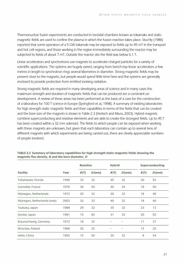
Strong magnetic fields are required in many developing areas of science and in many cases the maximum strength and duration of magnetic fields that can be produced are a constraint on development. A review of these areas has been performed as the basis of a case for the construction of a laboratory for 100 T science in Europe (Springford et al, 1998). A summary of existing laboratories for high strength static magnetic fields and their capabilities in terms of the fields that can be created and the bore size of the magnets is shown in Table 2.3 (Herlach and Miura, 2003). Hybrid magnets combine superconducting and resistive elements and are able to create the strongest fields. Up to 45 T has been created within a 32 mm solenoid. The fields to which people can be exposed when working with these magnets are unknown, but given that each laboratory can contain up to several tens of different magnets with which experiments are being carried out, there are clearly appreciable numbers of people involved.
TABLE 2.3 Summary of laboratory capabilities for high strength static magnetic fields showing the magnetic flux density, B, and the bore diameter, D
Resistive Hybrid Superconducting
Facility Year B (T) D (mm) B (T) D (mm) B (T) D (mm)
Tallahassee, Florida 1990 33 32 45 32 20 52
Grenoble, France 1970 30 50 40 34 18 50
Nijmegen, Netherlands 1972 20 32 30 32 18 40
Nijmegen, Netherlands (new) 2003 33 32 40 32 18 40
Tsukuba, Japan 1988 29 32 35 32 23 13
Sendai, Japan 1981 15 82 31 32 20 52
Braunschweig, Germany 1972 18 32 – – 11 37
Wroclaw, Poland 1968 20 25 – – 15 20
Hefei, China 1992 15 50 20 32 8 54
2 S O U R C E S , E X P O S U R E S A N D M E A S U R E M E N T S
28
2.5 Measurement equipment
2.5.1 General aspects
A variety of different technologies have been developed to measure magnetic fields and some of the longer established technologies have been reviewed by Lenz (1990). Developments continue and, in particular, sensors based on magnetoresistive mechanisms have been refined in recent years. This section describes the two types of sensor that are most commonly used to measure static magnetic fields – for example, when measuring the geomagnetic field or performing surveys around occupational sources.
Most magnetic field sensors require their sensing element to be aligned with the field in order to make a measurement, but often a surveyor will not know the direction of the field that is being measured. For this reason, many magnetic field measuring instruments contain three orthogonal sensors whose outputs are combined in order to yield the resultant magnetic field magnitude irrespective of the instrument orientation. The spatial resolution of a probe is also an important factor since large probes cannot resolve fine spatial detail in the field structure and will tend to average the field over the sensor volume. Sensor size is an important factor in determining the closest distance of approach to a source at which a measurement can be made.
Magnetic field sensors can be combined with data-loggers and made small enough to be worn on the body in order to monitor personal exposure of workers to static magnetic fields. One such device uses a novel solution to monitor exposure of MRI workers both to strong static fields and to small variations in those fields as the workers move within a field gradient (Crozier, 2007). The device contains Hall effect sensors to monitor the strong static field and its slower variations, and coil-based sensors that produce voltages proportional to rates of change in magnetic field associated with frequencies up to the kilohertz region, but which are insensitive to the static field.
2.5.2 Fluxgate magnetometers
Fluxgate magnetometers are common elements of laboratory and survey measurement instruments for magnetic fields in the range 0.1 nT to 10 mT and with bandwidths up to around 10 kHz. The principle of operation can be illustrated by considering a ferrite core around which there are primary and secondary windings, as shown in Figure 2.5. An AC signal is applied to the primary winding and used to saturate the core in alternate directions. The current induced in the secondary is monitored and it is possible to identify the onset of the non-linear response that occurs when the core saturates. In the absence of an applied external magnetic field, the core saturates at an equal primary current in both directions; however, this is not the case when there is an external applied magnetic field. The applied field adds to the field induced by the primary and so causes the ferrite core to saturate at different current levels when the primary current is applied in different directions. This is the basis of the measurement.
A practical survey instrument containing three orthogonal fluxgate magnetometer sensors is shown in Figure 2.6. The instrument provides voltage outputs in proportion to the three field components and these can be connected to an analogue to digital converter card used with a personal computer in order to display the field components or their resultant on the screen, eg as a function of time.
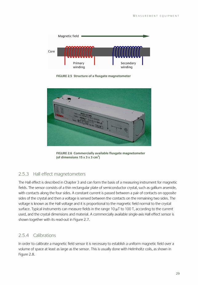
M E A S U R E M E N T E Q U I P M E N T
29
FIGURE 2.5 Structure of a fluxgate magnetometer
FIGURE 2.6 Commercially available fluxgate magnetometer (of dimensions 15 x 3 x 3 cm3)
2.5.3 Hall effect magnetometers
The Hall effect is described in Chapter 3 and can form the basis of a measuring instrument for magnetic fields. The sensor consists of a thin rectangular plate of semiconductor crystal, such as gallium arsenide, with contacts along the four sides. A constant current is passed between a pair of contacts on opposite sides of the crystal and then a voltage is sensed between the contacts on the remaining two sides. The voltage is known as the Hall voltage and it is proportional to the magnetic field normal to the crystal surface. Typical instruments can measure fields in the range 10 μT to 100 T, according to the current used, and the crystal dimensions and material. A commercially available single-axis Hall effect sensor is shown together with its read-out in Figure 2.7.
2.5.4 Calibrations
In order to calibrate a magnetic field sensor it is necessary to establish a uniform magnetic field over a volume of space at least as large as the sensor. This is usually done with Helmholtz coils, as shown in Figure 2.8.
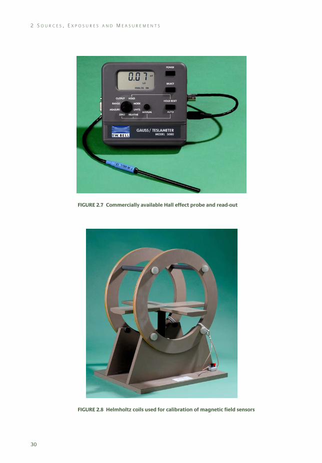
2 S O U R C E S , E X P O S U R E S A N D M E A S U R E M E N T S
30
FIGURE 2.7 Commercially available Hall effect probe and read-out
FIGURE 2.8 Helmholtz coils used for calibration of magnetic field sensors
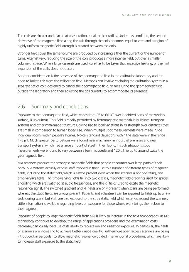
S U M M A R Y A N D C O N C L U S I O N S
31
The coils are circular and placed at a separation equal to their radius. Under this condition, the second derivative of the magnetic field along the axis through the coils becomes equal to zero and a region of highly uniform magnetic field strength is created between the coils.
Stronger fields over the same volume are produced by increasing either the current or the number of turns. Alternatively, reducing the size of the coils produces a more intense field, but over a smaller volume of space. Where large currents are used, care has to be taken that excessive heating, or thermal expansion of the coils, does not occur.
Another consideration is the presence of the geomagnetic field in the calibration laboratory and the need to isolate this from the calibration field. Methods can involve enclosing the calibration system in a separate set of coils designed to cancel the geomagnetic field, or measuring the geomagnetic field outside the laboratory and then adjusting the coil currents to accommodate its presence.
2.6 Summary and conclusions
Exposure to the geomagnetic field, which varies from 25 to 60 μT over inhabited parts of the world’s surface, is ubiquitous. This field is readily perturbed by ferromagnetic materials in buildings, transport systems and other man-made structures, giving rise to local variations in its strength over distances that are small in comparison to human body size. When multiple spot measurements were made inside individual rooms within people’s homes, typical standard deviations within the data were in the range 1–3 μT. Much greater perturbations were found near machinery in industrial premises and near transport systems, which had a large amount of steel in their fabric. In such situations, spot measurements were found to vary between a few microtesla and 120 μT, ie up to around twice the geomagnetic field.
MRI scanners produce the strongest magnetic fields that people encounter over large parts of their body. MRI systems actually expose staff involved in their use to a number of different types of magnetic fields, including the static field, which is always present even when the scanner is not operating, and time-varying fields. The time-varying fields fall into two classes, magnetic field gradients used for spatial encoding which are switched at audio frequencies, and the RF fields used to excite the magnetic resonance signal. The switched gradient and RF fields are only present when scans are being performed, whereas the static fields are always present. Patients and volunteers can be exposed to fields up to a few tesla during scans, but staff are also exposed to the stray static field which extends around the scanner. Little information is available regarding levels of exposure for those whose work brings them close to the magnets.
Exposure of people to large magnetic fields from MRI is likely to increase in the next few decades, as MRI technology continues to develop, the range of applications broadens and the examination costs decrease, particularly because of its ability to replace ionising radiation exposure. In particular, the fields of scanners are increasing to achieve better image quality. Furthermore open access scanners are being introduced, in particular to allow magnetic resonance guided interventional procedures, which are likely to increase staff exposure to the static field.
2 S O U R C E S , E X P O S U R E S A N D M E A S U R E M E N T S
32
There are few other man-made sources and situations that can give rise to static magnetic field exposure at levels appreciably above the geomagnetic field. There have been several systematic investigations of exposures in industrial electrolysis facilities and these indicate exposures of staff working near the cells and conductors of a few millitesla throughout the working day, with exposures up to around 20 mT being possible in some places.
Some arc welding and resistance welding sources use DC supplies and so give rise to static fields in their vicinity. Operators of arc welding equipment, which uses currents up to around 600 A, often drape the cable over their shoulder and fields of a few millitesla have been measured at 1 cm from the cable. Resistance welding uses higher currents, up to 10 kA or more, and it seems that exposure up to millitesla levels is also possible, although there are few reported data.
Some transport systems, such as certain types of trains, contain DC motors and so have sources of static fields onboard. What measurements are available suggest that the fields at most locations are essentially similar to typical perturbed geomagnetic fields. However, air-cored smoothing inductors beneath the floors of some trains have been found to produce fields over 10 mT immediately above them at floor level.
The above source categories (welding, electrolysis and transport systems not powered by batteries) use DC derived from rectification of AC supplies with or without some degree of smoothing of the current waveform applied. As a consequence, ELF AC fields with frequency components that are harmonics of the AC signal are produced along with the static fields. There are very few situations where static fields are produced without AC fields present and these include applications such as MRI, HVDC power lines and a range of scientific applications using electromagnets to deflect particle and plasma beams.
For practical exposure assessment purposes static magnetic fields are usually measured with a fluxgate magnetometer or a Hall effect sensor, and instruments are on the market based on either of these technologies. Fluxgate magnetometers are the more sensitive, typically covering 0.1 nT to 10 mT, and Hall effect probes typically cover 10 μT to 100 T.
2.7 References Allen SG, Blackwell RP, Chadwick PJ, Driscoll CMH, Pearson AJ, Unsworth C and Whillock MJ (1994). Review of
occupational exposure to optical radiation and electric and magnetic fields with regard to the proposed CEC Physical Agents Directive. Chilton, NRPB-R265.
Bacher K, Bogaert E, Lapere R, de Wolf D and Thierens H (2005). Patient-specific dose and radiation risk estimation in pediatric cardiac catheterization. Circulation, 111, 83–9.
Bowman JD and Methner MM (2000). Hazard surveillance for industrial magnetic fields: II. Field characteristics from waveform measurements. Ann Occup Hyg, 44, 615–33.
Bloch F (1946). Nuclear induction. Phys Rev, 70(7–8), 460–74.
Bradley J (2005). Monitoring occupational exposure to static magnetic fields in MRI units. London, Institute of Physics and Engineering in Medicine.
Cavin ID, Glover PM, Bowtell RW and Gowland PA (2007). Thresholds for perceiving metallic taste at high magnetic field. J Magn Reson Imaging, 26(5), 1357–61.
Chadwick P and Lowes F (1998). Magnetic fields on British trains. Ann Occup Hyg, 42(5), 331–5.
R E F E R E N C E S
33
Cooper TG (2002). Occupational exposure to electric and magnetic fields in the context of the ICNIRP guidelines. Chilton, NRPB-W24.
Crozier S (2007). An investigation into occupational exposure to electromagnetic fields for personnel working with and around magnetic resonance imaging equipment. Annex to Assessment of Electromagnetic Fields around Magnetic Resonance Imaging (MRI) Equipment. Sudbury, HSE Books, RR570.
de Wilde J (2004). Personal communication, MagNET. London, Medicines and Healthcare products Regulatory Agency.
Dietrich FM and Jacobs WL (1999). Survey and Assessment of Electric and Magnetic Field (EMF) Public Exposure in the Transportation Environment. US Department of Transportation, Federal Railroad Administration (Report nr PB99-130908). http://ntlsearch.bts.gov/tris/record/tris/00804485.html.
EC (European Commission) (1996). Non-ionizing radiation sources, exposure and health effects. Employment and Social Affairs. Luxembourg, European Commission.
Hall WA, Liu H, Martin AJ, Pozza CH, Maxwell RE and Truwit CL (2000). Safety, efficacy, and functionality of high-field strength interventional magnetic resonance imaging for neurosurgery. Neurosurgery, 46(3), 632–41.
Hall WA, Kowalik K, Kucharczk J and Truwit CL (2001). Cost effectiveness of intraoperative MR for tumor resection. Neurosurgery, 49(s), 518–19.
Hall WA, Liu H and Truwit CL (2005). Functional magnetic resonance imaging-guided resection of low-grade gliomas. Surg Neurol, 64(1), 20–27.
Haskal ZJ (2004). Cataract In interventional radiology – an occupational hazard? Presented at Society for Interventional Radiology, 29th Annual Scientific Meeting, Phoenix.
Herlach F and Miura N (2003). High Magnetic Fields: Science and Technology. Volume 1: Magnet Technology and Experimental Techniques. Singapore, World Scientific Publishing.
ICRP (2001). Avoidance of radiation injuries from medical interventional procedures. ICRP Publication 85. Ann ICRP, 30(2).
Kaune WT, Banks RS, Linet MS, Hatch EE, Kleinerman RA, Wacholder S, Tarone RE and Haines C (2001). Static magnetic field measurements in residences in relation to resonance hypotheses of interactions between power-frequency magnetic fields and humans. Bioelectromagnetics, 22(5), 294–305.
Krautmacher C, Willinek WA, Tschampa HJ, Born M, Traber F, Gieseke J, Textor HJ, Schild HH and Kuhl CK (2005). Brain tumors: full- and half-dose contrast-enhanced MR imaging at 3.0 T compared with 1.5 T – initial experience. Radiology, 237(3), 1014–19.
Kucharczyk J, Hall WA, Broaddus WC, Gillies GT and Truwit CL (2001). Cost-efficacy of MR-guided neurointerventions. Neuroimaging Clin N Am, 11(4), 767–72, xii.
Lauterbur PC (1973). Image formation by induced local interactions – examples employing nuclear magnetic-resonance. Nature, 242(5394), 190–91.
Lenz JE (1990). A review of magnetic sensors. Proc IEEE, 78(6), 973–89.
Mansfield P and Grannell PK (1973). NMR diffraction in solids. J Phys C – Solid State Phys, 6(22), L422–6.
Marsh JL, Armstrong TJ, Jacobson AP and Smith RG (1982). Health effect of occupational exposure to steady magnetic fields. Am Ind Hyg Assoc J, 43, 387–94.
Martin AJ, Hall WA, Liu H, Pozza CH, Michel E, Casey SO, Maxwell RE and Truwit CL (2000). Brain tumor resection: intraoperative monitoring with high-field-strength MR imaging – initial results. Radiology, 215(1), 221–8.
Martin AJ, Weber O, Saloner D, Higashida R, Wilson M, Saeed M and Higgins C (2002). Application of MR technology to endovascular interventions in an XMR suite. Medicamundi, 46(3), 28–34.
Melton GB (2005). Measurement and analysis of magnetic fields from welding processes. Health and Safety Executive (UK) Research Report 338. http://www.hse.gov.uk/research/rrhtm/rr338.htm.
Moen BE, Drablos PA, Pedersen S, Sjoen M and Thommesen G (1995). Symptoms of the musculoskeletal system and exposure to magnetic fields in an aluminium plant. Occup Environ Med, 52(8), 524–7.
Moen BE, Drablos PA, Pedersen S, Sjoen M and Thommesen G (1996). Absence of relation between sick leave caused by musculoskeletal disorders and exposure to magnetic fields in aluminum plant. Bioelectromagnetics, 17, 37–43.
Moore EA, Scurr E and Price D (2006). Potential impact of the EU PAD (EMF) on MR clinical practice in the UK. Presented at IPEM MR Safety Update Meeting, London, October 2006.
2 S O U R C E S , E X P O S U R E S A N D M E A S U R E M E N T S
34
Mur J-M, Wild P, Rapp R, Vautrin J-P and Coulon J-P (1998). Demographic evaluation of the fertility of aluminium industry workers: influence of exposure to heat and static magnetic fields. Hum Reprod, 13(7), 2016–19.
NGDC (2006). http://www.ngdc.noaa.gov/ngdc.html. National Geophysical Data Center.
Pastides H (1992). A characterization of occupational static magnetic field exposures at a diaphragm-cell and mercury-cell chlor-alkali facility. Appl Occup Environ Hyg, 7(1), 42–8.
Paterson A and Frush DP (2007). Dose reduction in paediatric MDCT: general principles. Clin Radiol, 62(6), 507–17.
Razavi R, Hill DL, Keevil SF, Miquel ME, Muthurangu V, Hegde S, Rhode K, Barnett M, van Vaals J, Hawkes DJ and Baker E (2003). Cardiac catheterisation guided by MRI in children and adults with congenital heart disease. Lancet, 362(9399), 1877–82.
Riches SF, Collins DJ, Scuffham JW and Leach MO (2007). EU Directive 2004/40: field measurements of a 1.5 T clinical MR scanner. Br J Radiol, 80(954), 483–7.
Skotte JH and Hjøllund HI (1997). Exposure of welders and other metal workers to ELF magnetic fields. Bioelectromagnetics, 18(7), 470–77.
Springford M, Challis LJ and Karow HU, eds (1998). The scientific case for a European laboratory for 100 tesla science. Strasbourg, European Science Foundation Study Report.
Stuchly M (1986). Human exposure to static and time-varying magnetic fields. Health Phys, 51(2), 215–25.
Swanson J (1994). Measurements of static magnetic fields in homes in the UK and their implication for epidemiological studies of exposure to alternating magnetic fields. J Radiol Prot, 14, 67–75.
WHO (2006). Static Fields. Environmental Health Criteria 232. Geneva, World Health Organization. http://www.who.int/peh-emf/publications/reports/ehcstatic/en/index.html.
35
3 Mechanisms for Biological Interaction
Static magnetic fields interact with moving charged particles, such as ions, and with magnetic moments (dipoles) arising from the orbital motion or spin of the electrons in an atom. Many nuclei also have moments, although these are much smaller than those associated with electrons. Interactions with charges are often referred to as electrodynamic and those with magnetic moments as magnetomechanical. Recent reviews of interaction mechanisms are cited by Schenck (2005). Interaction mechanisms with time-dependent fields will not be considered here unless they are the result of body motion.
3.1 Electrodynamic interactions
3.1.1 Form of the interaction
Magnetic fields interact electrodynamically with charges if they are moving, ie if there are electric currents present. As noted earlier, the force F on a charge q moving with velocity v in a uniform magnetic field B is given by the magnetic part of the Lorentz force
F = qv x B (3.1)
If ϑ is the angle between the directions of B and v , the force F has magnitude qvB sin ϑ and is at right angles to both B and v . Hence the field only interacts if it has a component perpendicular to v .
So if a conductor containing n charges per unit volume is carrying a current of density J = nqv , a magnetic field perpendicular to J deflects the charges to one side. This continues, briefly, until the force on a charge E H q due to the transverse electric field E H generated by the charge separation (the Hall field) balances the Lorentz force qvB⊥, where B⊥ is the field component perpendicular to the current. Hence a magnetic field produces a potential difference V across the width d of the conductor of magnitude
V = E H d = vB⊥ (3.2)
Another effect of the Lorentz force is to increase the resistivity of the conductor. This should be a negligible effect for most biological tissue because of the low mobility μC of the charge carriers within it*.
If the field is non-uniform, there is also a force on a charge moving with velocity v parallel to B . This can be seen by choosing the reference frame to be that of the charge. In this frame, the charge is at rest while the magnetic field appears to be changing with time at a rate
dB /dt = v dB/dz (3.3)
* Mobility, μ C, is defined as the drift velocity a charge acquires in the direction of an electric field E of 1 V m–1. In a magnetic field B, the charge path between collisions becomes curved resulting in an increase in resistivity. The increase is, however, negligible if μ C B « 1 which is the case for values of B of interest since μ C < 10–7 m2 V–1 s for ions in biological tissue.
3 M E C H A N I S M S F O R B I O L O G I C A L I N T E R A C T I O N
36
where the field gradient, dB/dz, is taken to be in the same direction as B .
From Faraday’s law, the charge experiences an electric field given by
curl E = – dB /dt = – v dB/dz (3.4)
The electric field lines circulate around the direction of B so that, in a conducting material, the charges move around B resulting in current loops.
3.1.2 Currents in body tissue
Although most body tissue is electrically conducting, in the absence of an applied magnetic field current flow only occurs in particular components such as nerves and muscles and similar excitable tissues, such as pancreatic beta-cells. When a magnetic field is present, eddy currents can be induced in other tissues if they are moving relative to the field. This can happen either because of body movement (eg Liu et al, 2003) or because of the flow of blood in the heart and blood vessels such as the aorta (eg Kinouchi et al, 1996). The interaction of the induced currents in conducting fluid with a magnetic field is particularly complex and a full description of the magnetohydrodynamics, the resulting forces and motion, can only be obtained by solving or modelling the Navier-Stokes equation of fluid mechanics for the particular geometry. It is also necessary to specify the boundary conditions – for example, whether the containing walls of blood vessels are insulating, or are conducting so that current can flow into the surrounding tissue. The calculations have been carried out for field components normal to the blood vessels and no effects should occur for uniform fields parallel to the vessels.
While reliable, quantitative results for blood flow can only be obtained from the Navier-Stokes equation, an understanding of the nature of the interaction can be obtained by considering fluid flow in a large sheet in the x–y plane of thickness t . The fluid is assumed to have conductivity σ and to be moving along the y -direction with an average velocity v . When a magnetic field B is applied in the z -direction, a current is induced along the x -direction of density J = σBv. The size of the Lorentz force in the –y-direction on the current flowing through an area t dy = B J t dy per unit length. This leads to a pressure gradient dP B /dy = B J = σvB 2 which opposes the blood flow*.
The model can now be extended to a vessel of square cross-section t x t or of circular cross-section of radius a = t /2. The current and so the pressure gradient dP B /dy should be approximately the same as for the sheet if the walls and external tissue have the same electrical conductivity as the blood. If, however, they have a conductivity σW < σ, dP B /dy will be reduced by approximately σW/σ and the current flow into the surrounding tissue will have a density J = σW Bv . If the walls are insulating, the net induced current in the y -direction and so dP B /dy would become zero and no current would flow into the surrounding tissue. The effect of these electrodynamic effects on the fluid flow can be seen by comparing dP B /dy with the pressure gradient responsible for the flow, dP /dy = 8ηv/a 2 (Poiseuille’s law) where η is the viscosity of the fluid.
* The current flow also generates a magnetic field μ 0J t /2 around the sheet, where μ 0 is the permeability of free space, which leads to an inward pressure on all surfaces of P = (μ 0σv t ) 2B 2/8μ 0. This is, however, extremely small compared with the blood pressure and can safely be neglected.
M A G N E T O M E C H A N I C A L I N T E R A C T I O N S
37
3.2 Magnetomechanical interactions
Materials are inherently magnetic. In most, the electronic magnetic moments of atoms or molecules cancel out in the absence of an applied magnetic field and these materials are called diamagnetic. The cancellation is destroyed when a field B is applied and the atoms or molecules acquire small net magnetic moments proportional to B but in the opposite direction. The size of the moment can be written: m v = χ B /μ0, where m v is the magnetic moment per unit volume and χ, the diamagnetic susceptibility, is negative. Some materials, however, contain atoms or molecules that have non-zero magnetic moments m in the absence of an applied magnetic field. These are called paramagnetic and, in these, the moments tend to align along an applied field resulting in a net magnetic moment parallel to B . The biggest effects though occur in ferromagnetic or in ferrimagnetic * materials. In these, neighbouring moments of atoms or molecules are coupled together by exchange forces so that particles of these materials, such as ferrimagnetic magnetite (Fe3O4) which occurs in some biological tissue, have very large magnetic moments.
* The behaviour of ferrimagnetic materials is similar to that of ferromagnetic materials at a macroscopic level but there are differences at a microscopic level.
There is no force on a magnetic moment if the magnetic field is uniform. However, the moment experiences a torque
Γ = m x B (3.5)
which has magnitude mB sin β, where β is the angle between m and B . The direction of the torque, the axis of rotation of any subsequent motion, is perpendicular to both of them.
The interaction also leads to potential energy
Um = – mB (3.6)
of magnitude m B cos β.
The direction of paramagnetic moments tends to be randomised by thermal motion. The net degree of alignment depends therefore on how the magnetic energy, mB, compares with the thermal energy, k B T . For a body temperature around 310 K, k B T is around 4 10–21 J, so for B = 10 T, significant alignment should occur for moments m > 4 10–22 J T-1. This is appreciably greater than typical paramagnetic moments of around 10–23
J T–1 so only very small alignment should occur in paramagnetic materials at
body temperature in fields of 10 T. The moments of ferromagnetic particles or ferromagnetic particles such as magnetite are, however, large enough for their alignment in 10 T fields to be nearly complete.
The induced magnetic moments in most diamagnetic materials do not experience torques in magnetic fields since the moments are always antiparallel to the field. This is not the case, however, if the diamagnetic susceptibility is different in different directions as it can be in proteins or other macromolecules and the differences can be as large as 10%. In this situation, the potential energy is least when the direction of greatest susceptibility lies along the field. If this is not the case, the material experiences a torque and has potential energy
U = [(χ2 – χ1) /2μ0]VB 2 sin2 β (3.7)
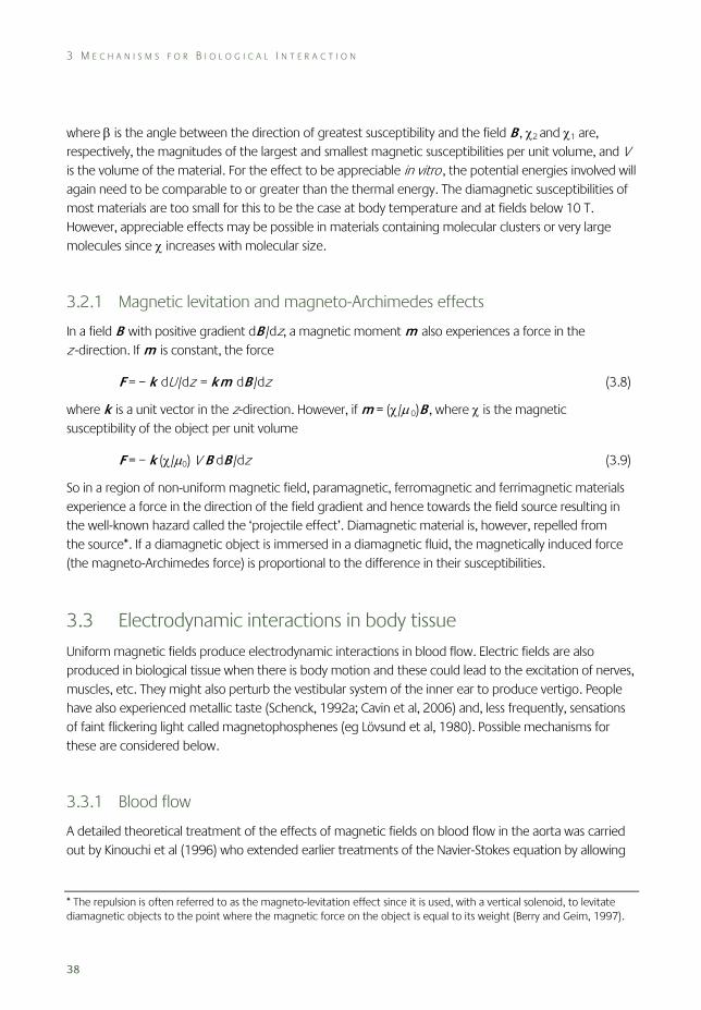
3 M E C H A N I S M S F O R B I O L O G I C A L I N T E R A C T I O N
38
where β is the angle between the direction of greatest susceptibility and the field B , χ2 and χ1 are, respectively, the magnitudes of the largest and smallest magnetic susceptibilities per unit volume, and V is the volume of the material. For the effect to be appreciable in vitro , the potential energies involved will again need to be comparable to or greater than the thermal energy. The diamagnetic susceptibilities of most materials are too small for this to be the case at body temperature and at fields below 10 T. However, appreciable effects may be possible in materials containing molecular clusters or very large molecules since χ increases with molecular size.
3.2.1 Magnetic levitation and magneto-Archimedes effects
In a field B with positive gradient dB /dz, a magnetic moment m also experiences a force in the z -direction. If m is constant, the force
F = – k dU/dz = km dB /dz (3.8)
where k is a unit vector in the z-direction. However, if m = (χ/μ0)B , where χ is the magnetic susceptibility of the object per unit volume
F = – k (χ/μ0) V B dB /dz (3.9)
So in a region of non-uniform magnetic field, paramagnetic, ferromagnetic and ferrimagnetic materials experience a force in the direction of the field gradient and hence towards the field source resulting in the well-known hazard called the ‘projectile effect’. Diamagnetic material is, however, repelled from the source*. If a diamagnetic object is immersed in a diamagnetic fluid, the magnetically induced force (the magneto-Archimedes force) is proportional to the difference in their susceptibilities.
3.3 Electrodynamic interactions in body tissue
Uniform magnetic fields produce electrodynamic interactions in blood flow. Electric fields are also produced in biological tissue when there is body motion and these could lead to the excitation of nerves, muscles, etc. They might also perturb the vestibular system of the inner ear to produce vertigo. People have also experienced metallic taste (Schenck, 1992a; Cavin et al, 2006) and, less frequently, sensations of faint flickering light called magnetophosphenes (eg Lövsund et al, 1980). Possible mechanisms for these are considered below.
3.3.1 Blood flow
A detailed theoretical treatment of the effects of magnetic fields on blood flow in the aorta was carried out by Kinouchi et al (1996) who extended earlier treatments of the Navier-Stokes equation by allowing
* The repulsion is often referred to as the magneto-levitation effect since it is used, with a vertical solenoid, to levitate diamagnetic objects to the point where the magnetic force on the object is equal to its weight (Berry and Geim, 1997).

E L E C T R O D Y N A M I C I N T E R A C T I O N S I N B O D Y T I S S U E
39
for the fact that the arterial walls and extravascular tissue are both conducting. They found that, for magnetic fields perpendicular to the blood flow, magnetohydrodynamic forces reduced the flow rate of blood by around 1% in 5 T, 5% in 10 T and 10% in 15 T. (Their calculations assumed the conductivity of blood, arterial walls and extravascular tissue to be 0.5, 0.15 and 0.2 S m–1, respectively, with blood viscosity η of 5 10–3 Pa s, average flow velocity of 0.6 m s–1 and vessel radius a of 0.01 m.) The reduction of 5% for a field of 10 T is, as expected, much greater than the upper bound of 0.2%* calculated for electrically insulating walls (Keltner et al, 1990).
In the simple model, dP B /dy = (σW/σ) σvB 2, so, for the parameters used by Kinouchi et al and putting σW = 0.175 S m–1 (the mean of the values used by these authors for the walls and extravascular tissue), dP B /dy = 7, 30 and 67.5 Pa m–1 for B = 5, 10 and 15 T, respectively. Since the pressure gradient dP/dy driving the flow = 8ηv/a 2 = 240 Pa m–1, the reductions in flow rate are 1, 4 and 10%, respectively. It is reassuring that these values are similar to those given by detailed calculation.
The flow of current from the blood vessels into the extravascular tissue may be of greater significance than the reduction in blood flow rate. The current density varies linearly with magnetic field and decreases with distance from the aorta. Kinouchi et al suggested that the sinoatrial node of the heart that controls cardiac pacing may be the region most sensitive to current and calculated that, for a field of 5 T, the current density in this region was around 100 mA m–2, around 10% of the maximum endogenous current from cardiac electrical activity. This rises to around 20% at 10 T. Holden (2005) suggested that the myocardium might be even more sensitive to field-induced current flow from the vessels on or in the heart tissue. He carried out a detailed analysis of the potential distribution around the heart and assessed the effects of the electric field on cardiac function using computational models of cardiac electrophysiology. He concluded that, while fields up to 8 T were unlikely to affect the heart rate and rhythm materially, this would not necessarily be the case for larger fields.
These changes in blood flow rate and current density calculated by Kinouchi et al (1996) are for magnetic fields perpendicular to the blood flow in the aorta and very much smaller changes would be expected for parallel fields. In most cases, the axial field is approximately parallel to the aorta when patients are lying inside an MRI magnet†. However, it is approximately perpendicular to the aortic arch so while the largest currents into the surrounding tissue would be expected there, this is further away from the sinoatrial node. The fields would also be approximately perpendicular to the aorta for people standing near the mouth of an MRI magnet but the field values would be appreciably smaller than those inside.
One further electrodynamic effect is associated with the charge separation that occurs across a blood vessel (Hall effect). This induces charge on the skin which has been seen in electrocardiograms (Togawa et al, 1967; Gaffey and Tenforde, 1981; Tenforde et al, 1983; Jehenson et al, 1988).
* There should in fact be no reduction for insulating walls as explained earlier (Section 3.1.2). † In general, the axial field B will have a gradient dB /dz. So, to satisfy the Maxwell equation div B = 0, there must also be a radial field gradient dB /dr present and hence a radial field. However, this would normally be much less than the axial field.
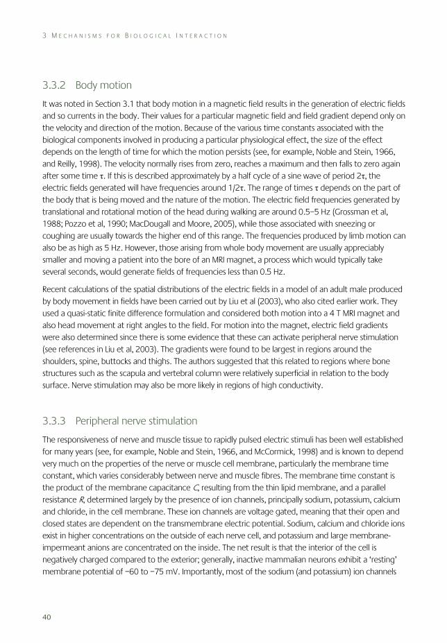
3 M E C H A N I S M S F O R B I O L O G I C A L I N T E R A C T I O N
40
3.3.2 Body motion
It was noted in Section 3.1 that body motion in a magnetic field results in the generation of electric fields and so currents in the body. Their values for a particular magnetic field and field gradient depend only on the velocity and direction of the motion. Because of the various time constants associated with the biological components involved in producing a particular physiological effect, the size of the effect depends on the length of time for which the motion persists (see, for example, Noble and Stein, 1966, and Reilly, 1998). The velocity normally rises from zero, reaches a maximum and then falls to zero again after some time τ. If this is described approximately by a half cycle of a sine wave of period 2τ, the electric fields generated will have frequencies around 1/2τ. The range of times τ depends on the part of the body that is being moved and the nature of the motion. The electric field frequencies generated by translational and rotational motion of the head during walking are around 0.5–5 Hz (Grossman et al, 1988; Pozzo et al, 1990; MacDougall and Moore, 2005), while those associated with sneezing or coughing are usually towards the higher end of this range. The frequencies produced by limb motion can also be as high as 5 Hz. However, those arising from whole body movement are usually appreciably smaller and moving a patient into the bore of an MRI magnet, a process which would typically take several seconds, would generate fields of frequencies less than 0.5 Hz.
Recent calculations of the spatial distributions of the electric fields in a model of an adult male produced by body movement in fields have been carried out by Liu et al (2003), who also cited earlier work. They used a quasi-static finite difference formulation and considered both motion into a 4 T MRI magnet and also head movement at right angles to the field. For motion into the magnet, electric field gradients were also determined since there is some evidence that these can activate peripheral nerve stimulation (see references in Liu et al, 2003). The gradients were found to be largest in regions around the shoulders, spine, buttocks and thighs. The authors suggested that this related to regions where bone structures such as the scapula and vertebral column were relatively superficial in relation to the body surface. Nerve stimulation may also be more likely in regions of high conductivity.
3.3.3 Peripheral nerve stimulation
The responsiveness of nerve and muscle tissue to rapidly pulsed electric stimuli has been well established for many years (see, for example, Noble and Stein, 1966, and McCormick, 1998) and is known to depend very much on the properties of the nerve or muscle cell membrane, particularly the membrane time constant, which varies considerably between nerve and muscle fibres. The membrane time constant is the product of the membrane capacitance C, resulting from the thin lipid membrane, and a parallel resistance R, determined largely by the presence of ion channels, principally sodium, potassium, calcium and chloride, in the cell membrane. These ion channels are voltage gated, meaning that their open and closed states are dependent on the transmembrane electric potential. Sodium, calcium and chloride ions exist in higher concentrations on the outside of each nerve cell, and potassium and large membrane-impermeant anions are concentrated on the inside. The net result is that the interior of the cell is negatively charged compared to the exterior; generally, inactive mammalian neurons exhibit a ‘resting’ membrane potential of –60 to –75 mV. Importantly, most of the sodium (and potassium) ion channels

E L E C T R O D Y N A M I C I N T E R A C T I O N S I N B O D Y T I S S U E
41
are closed, so that sodium ions are prevented from diffusing along their electrochemical gradient into the nerve cell thereby reducing (or depolarising) the transmembrane potential. If the resting potential difference across the nerve cell membrane is reduced – for example, by an applied electric potential – there is a transient voltage-dependent increase in the number of sodium ion channels open. When the depolarisation exceeds a critical threshold value, typically of around 10–15 mV, the opening of the voltage-gated sodium ion channels becomes self-sustaining, resulting in the transmembrane voltage becoming transiently positive before the slower acting voltage-gated potassium ion channels open and restore the resting potential. This wave of depolarisation, termed an action potential, propagates along the nerve axon, resulting, for example, in muscle contraction or a sensation, depending on whether the stimulated nerve was a motor (or efferent) nerve, or a sensory (or afferent) nerve.
The threshold electric field needed to produce an action potential is frequency dependent. At low frequencies, most of the potential difference produced by the field occurs across the cell membranes since their resistance R is larger than that of other parts of the cells and surrounding fluid. As the frequency ν increases, the parallel component of the impedance of the membrane, 1/ωC (where ω = 2πν ), resulting from its capacitance C , reduces its overall impedance. This results in a decrease in the voltage across a membrane and so increases the threshold electric field for depolarisation. It rises to twice its low frequency value by ω = 1/RC, which defines the time constant RC referred to earlier. For myelinated nerve fibres of the peripheral and central nervous system, which have membrane time constants of around 150 μs resulting from the presence of a fatty myelin sheath, the threshold increases to twice its low frequency value by around 7000 Hz. However, for cardiac stimulation, this is determined by the comparatively long membrane time constant of 3 ms and in this case the threshold becomes twice its low frequency value at around 300 Hz. At intermediate frequencies well below these values, the threshold remains constant down to about 10 Hz. It then begins to rise as the frequency is lowered as a result of the accommodation process caused by the inactivation of the voltage-gated sodium ion channels (Bezanilla, 2000).
The electric fields produced by a changing magnetic field are proportional to the rate of change of the field with time, dB/dt , so it is expected that peripheral nerve and muscle stimulation should occur above some threshold value of dB/dt . The present report is only concerned with stimulation effects caused by movement in static fields for which dB /dt = v dB/dz , the product of the spatial field gradient and the velocity of the body along the gradient and, from the discussion above, it would appear that the threshold value for stimulation would depend on the length of time that the motion persists. Information on the thresholds can be obtained from studies of time-dependent fields but their values will only be comparable to those for body motion if the electric field frequencies were broadly similar.
A study of 84 volunteers (Bourland et al, 1999) showed that the average sensation thresholds for 1 ms pulses were around 15 T s–1 for field changes normal to B and 26 T s–1 for changes parallel to B . The frequencies of the electric fields in this case will be around 1000 Hz. This lies within the intermediate range where the thresholds for all but cardiac stimulation are constant and at their minimum values.
Glover et al (2007) reported that values of dB/dt up to 20 T s–1 can be generated by fast angular rotations of the head just inside the magnet bore of a 7 T MRI magnet at the University of Nottingham.
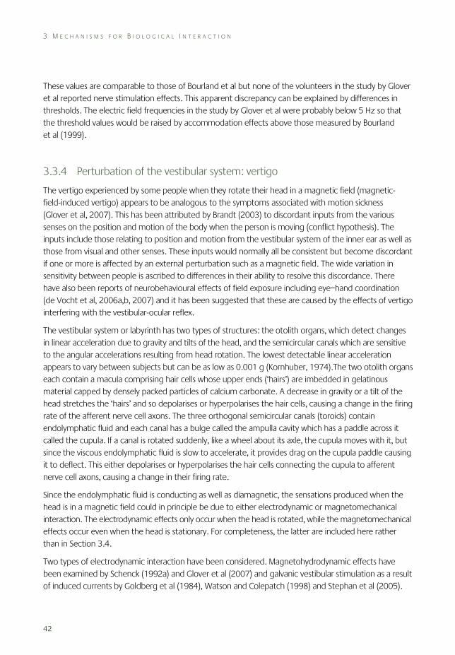
3 M E C H A N I S M S F O R B I O L O G I C A L I N T E R A C T I O N
42
These values are comparable to those of Bourland et al but none of the volunteers in the study by Glover et al reported nerve stimulation effects. This apparent discrepancy can be explained by differences in thresholds. The electric field frequencies in the study by Glover et al were probably below 5 Hz so that the threshold values would be raised by accommodation effects above those measured by Bourland et al (1999).
3.3.4 Perturbation of the vestibular system: vertigo
The vertigo experienced by some people when they rotate their head in a magnetic field (magnetic-field-induced vertigo) appears to be analogous to the symptoms associated with motion sickness (Glover et al, 2007). This has been attributed by Brandt (2003) to discordant inputs from the various senses on the position and motion of the body when the person is moving (conflict hypothesis). The inputs include those relating to position and motion from the vestibular system of the inner ear as well as those from visual and other senses. These inputs would normally all be consistent but become discordant if one or more is affected by an external perturbation such as a magnetic field. The wide variation in sensitivity between people is ascribed to differences in their ability to resolve this discordance. There have also been reports of neurobehavioural effects of field exposure including eye–hand coordination (de Vocht et al, 2006a,b, 2007) and it has been suggested that these are caused by the effects of vertigo interfering with the vestibular-ocular reflex.
The vestibular system or labyrinth has two types of structures: the otolith organs, which detect changes in linear acceleration due to gravity and tilts of the head, and the semicircular canals which are sensitive to the angular accelerations resulting from head rotation. The lowest detectable linear acceleration appears to vary between subjects but can be as low as 0.001 g (Kornhuber, 1974).The two otolith organs each contain a macula comprising hair cells whose upper ends (‘hairs’) are imbedded in gelatinous material capped by densely packed particles of calcium carbonate. A decrease in gravity or a tilt of the head stretches the ‘hairs’ and so depolarises or hyperpolarises the hair cells, causing a change in the firing rate of the afferent nerve cell axons. The three orthogonal semicircular canals (toroids) contain endolymphatic fluid and each canal has a bulge called the ampulla cavity which has a paddle across it called the cupula. If a canal is rotated suddenly, like a wheel about its axle, the cupula moves with it, but since the viscous endolymphatic fluid is slow to accelerate, it provides drag on the cupula paddle causing it to deflect. This either depolarises or hyperpolarises the hair cells connecting the cupula to afferent nerve cell axons, causing a change in their firing rate.
Since the endolymphatic fluid is conducting as well as diamagnetic, the sensations produced when the head is in a magnetic field could in principle be due to either electrodynamic or magnetomechanical interaction. The electrodynamic effects only occur when the head is rotated, while the magnetomechanical effects occur even when the head is stationary. For completeness, the latter are included here rather than in Section 3.4.
Two types of electrodynamic interaction have been considered. Magnetohydrodynamic effects have been examined by Schenck (1992a) and Glover et al (2007) and galvanic vestibular stimulation as a result of induced currents by Goldberg et al (1984), Watson and Colepatch (1998) and Stephan et al (2005).
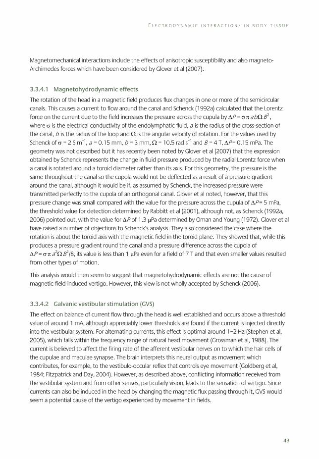
E L E C T R O D Y N A M I C I N T E R A C T I O N S I N B O D Y T I S S U E
43
Magnetomechanical interactions include the effects of anisotropic susceptibility and also magneto-Archimedes forces which have been considered by Glover et al (2007).
3.3.4.1 Magnetohydrodynamic effects
The rotation of the head in a magnetic field produces flux changes in one or more of the semicircular canals. This causes a current to flow around the canal and Schenck (1992a) calculated that the Lorentz force on the current due to the field increases the pressure across the cupula by ΔP = σπabΩB 2 , where σ is the electrical conductivity of the endolymphatic fluid, a is the radius of the cross-section of the canal, b is the radius of the loop and Ω is the angular velocity of rotation. For the values used by Schenck of σ = 2 S m–1, a = 0.15 mm, b = 3 mm, Ω = 10.5 rad s–1 and B = 4 T, ΔP = 0.15 mPa. The geometry was not described but it has recently been noted by Glover et al (2007) that the expression obtained by Schenck represents the change in fluid pressure produced by the radial Lorentz force when a canal is rotated around a toroid diameter rather than its axis. For this geometry, the pressure is the same throughout the canal so the cupola would not be deflected as a result of a pressure gradient around the canal, although it would be if, as assumed by Schenck, the increased pressure were transmitted perfectly to the cupola of an orthogonal canal. Glover et al noted, however, that this pressure change was small compared with the value for the pressure across the cupula of ΔP = 5 mPa, the threshold value for detection determined by Rabbitt et al (2001), although not, as Schenck (1992a, 2006) pointed out, with the value for ΔP of 1.3 μPa determined by Oman and Young (1972). Glover et al have raised a number of objections to Schenck’s analysis. They also considered the case where the rotation is about the toroid axis with the magnetic field in the toroid plane. They showed that, while this produces a pressure gradient round the canal and a pressure difference across the cupola of ΔP = σπa 2ΩB 2/8, its value is less than 1 μPa even for a field of 7 T and that even smaller values resulted from other types of motion.
This analysis would then seem to suggest that magnetohydrodynamic effects are not the cause of magnetic-field-induced vertigo. However, this view is not wholly accepted by Schenck (2006).
3.3.4.2 Galvanic vestibular stimulation (GVS)
The effect on balance of current flow through the head is well established and occurs above a threshold value of around 1 mA, although appreciably lower thresholds are found if the current is injected directly into the vestibular system. For alternating currents, this effect is optimal around 1–2 Hz (Stephen et al, 2005), which falls within the frequency range of natural head movement (Grossman et al, 1988). The current is believed to affect the firing rate of the afferent vestibular nerves on to which the hair cells of the cupulae and maculae synapse. The brain interprets this neural output as movement which contributes, for example, to the vestibulo-occular reflex that controls eye movement (Goldberg et al, 1984; Fitzpatrick and Day, 2004). However, as described above, conflicting information received from the vestibular system and from other senses, particularly vision, leads to the sensation of vertigo. Since currents can also be induced in the head by changing the magnetic flux passing through it, GVS would seem a potential cause of the vertigo experienced by movement in fields.
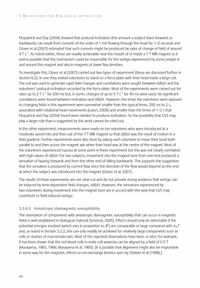
3 M E C H A N I S M S F O R B I O L O G I C A L I N T E R A C T I O N
44
Fitzpatrick and Day (2004) showed that postural inclination (the amount a subject leans forwards or backwards) can result from currents of the order of 1 mA flowing through the head for 1–2 seconds and Glover et al (2007) estimated that such currents might be produced by rates of change of field of around 4 T s–1. As noted earlier, these are readily achievable near the mouth of or inside a 7 T MRI magnet so it seems possible that this mechanism could be responsible for the vertigo experienced by some people in and around this magnet and also in magnets of lower flux densities.
To investigate this, Glover et al (2007) carried out two types of experiment (these are discussed further in Section 6.2). In one they invited volunteers to stand on a force-plate with their head inside a large coil. The coil was used to generate rapid field changes and correlations were sought between dB/dt and the volunteers’ postural inclination recorded by the force-plate. Most of the experiments were carried out for rates up to 2 T s–1 for 200 ms but, in some, changes of up to 5 T s–1 for 40 ms were used. No significant correlations were found between inclination and dB/dt . However, the times the volunteers were exposed to changing fields in this experiment were somewhat smaller than the typical times, 200 ms to 2 s, associated with rotational head movements (Luxon, 2006) and smaller than the times of 1–2 s that Fitzpatrick and Day (2004) found were needed to produce inclination. So the possibility that GVS may play a larger role than is suggested by this work cannot be ruled out.
In the other experiment, measurements were made on ten volunteers who were introduced at a moderate speed into and then out of the 7 T MRI magnet so that dB/dt was the result of motion in a field gradient. Further experiments were also done by asking each volunteer to move their head both parallel to and then across the magnet axis when their head was at the centre of the magnet. Most of the volunteers experienced nausea at some point in these experiment but this was not clearly correlated with high values of dB/dt. For two subjects, movement into the magnet bore from one end produced a sensation of tipping forwards and from the other end of falling backwards. This supports the suggestion that the sensation is produced by current flow since the direction of the flow would depend on the end at which the subject was introduced into the magnet (Glover et al, 2007).
The results of these experiments are not clear-cut and do not provide strong evidence that vertigo can be induced by time-dependent field changes, dB/dt . However, the sensations experienced by two volunteers during movement into the magnet bore are in accord with the view that GVS may contribute to field-induced vertigo.
3.3.4.3 Anisotropic diamagnetic susceptibility
The orientation of components with anisotropic diamagnetic susceptibility that can occur in magnetic fields is well established in biological material (Schenck, 2005). Effects should only be detectable if the potential energies involved (which vary in proportion to B 2) are comparable or large compared with k B T and, as noted in Section 3.2.2, this can only readily be achieved for relatively large components such as cells or clusters of macromolecules. Most of the reported observations have been in vitro ; for example, it has been shown that the red blood cells in sickle cell anaemia can be aligned by a field of 0.5 T (Murayama, 1965, 1966; Murayama et al, 1965). [It is possible that alignment might also be responsible in some way for the magnetic effects on ion-exchange kinetics seen by Oshitari et al (1998).]
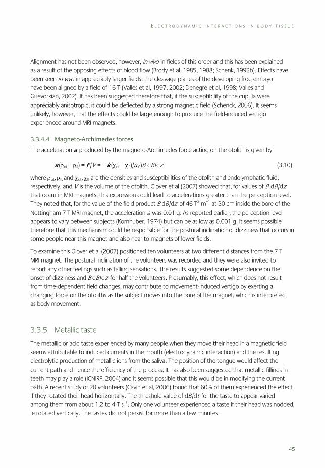
E L E C T R O D Y N A M I C I N T E R A C T I O N S I N B O D Y T I S S U E
45
Alignment has not been observed, however, in vivo in fields of this order and this has been explained as a result of the opposing effects of blood flow (Brody et al, 1985, 1988; Schenk, 1992b). Effects have been seen in vivo in appreciably larger fields: the cleavage planes of the developing frog embryo have been aligned by a field of 16 T (Valles et al, 1997, 2002; Denegre et al, 1998; Valles and Guevorkian, 2002). It has been suggested therefore that, if the susceptibility of the cupula were appreciably anisotropic, it could be deflected by a strong magnetic field (Schenck, 2006). It seems unlikely, however, that the effects could be large enough to produce the field-induced vertigo experienced around MRI magnets.
3.3.4.4 Magneto-Archimedes forces
The acceleration a produced by the magneto-Archimedes force acting on the otolith is given by
a (ρot – ρfl) = F /V = – k (χot – χfl)/μ0)B dB/dz (3.10)
where ρot, ρfl, and χot, χfl are the densities and susceptibilities of the otolith and endolymphatic fluid, respectively, and V is the volume of the otolith. Glover et al (2007) showed that, for values of B dB/dz that occur in MRI magnets, this expression could lead to accelerations greater than the perception level. They noted that, for the value of the field product B dB/dz of 46 T2 m–1 at 30 cm inside the bore of the Nottingham 7 T MRI magnet, the acceleration a was 0.01 g. As reported earlier, the perception level appears to vary between subjects (Kornhuber, 1974) but can be as low as 0.001 g. It seems possible therefore that this mechanism could be responsible for the postural inclination or dizziness that occurs in some people near this magnet and also near to magnets of lower fields.
To examine this Glover et al (2007) positioned ten volunteers at two different distances from the 7 T MRI magnet. The postural inclination of the volunteers was recorded and they were also invited to report any other feelings such as falling sensations. The results suggested some dependence on the onset of dizziness and B dB/dz for half the volunteers. Presumably, this effect, which does not result from time-dependent field changes, may contribute to movement-induced vertigo by exerting a changing force on the otoliths as the subject moves into the bore of the magnet, which is interpreted as body movement.
3.3.5 Metallic taste
The metallic or acid taste experienced by many people when they move their head in a magnetic field seems attributable to induced currents in the mouth (electrodynamic interaction) and the resulting electrolytic production of metallic ions from the saliva. The position of the tongue would affect the current path and hence the efficiency of the process. It has also been suggested that metallic fillings in teeth may play a role (ICNIRP, 2004) and it seems possible that this would be in modifying the current path. A recent study of 20 volunteers (Cavin et al, 2006) found that 60% of them experienced the effect if they rotated their head horizontally. The threshold value of dB/dt for the taste to appear varied among them from about 1.2 to 4 T s–1. Only one volunteer experienced a taste if their head was nodded, ie rotated vertically. The tastes did not persist for more than a few minutes.

3 M E C H A N I S M S F O R B I O L O G I C A L I N T E R A C T I O N
46
3.3.6 Magnetophosphenes
A phosphene is defined as a visual sensation generated by stimuli other than photons and the term magnetophosphene refers to the sensation produced by time-varying magnetic fields. These are usually sensed as faint flickering lights in the peripheral parts of the visual field and first appear to have been investigated by d’Arsonval (1896). Experiments by Barlow et al (1947) indicated that the light sensations were produced by the direct stimulation of excitable cells in the retina by the induced electric fields; similar effects can be induced by weak electric currents applied to the head (Adrian, 1977). However, the details of the mechanism have not yet been established. When the background illumination was low, the threshold value for light sensations was found to be around 1.5 T s–1 at 20–25 Hz, rising at higher and lower stimulus frequencies (Lövsund et al, 1980) but this minimum dB/dt threshold value increased somewhat with illumination. The effect disappeared once the time-varying fields stopped. Maximum sensitivity occurs at frequencies somewhat higher then those associated with typical head movements but not of all eye movements. Discussions of possible mechanisms have been given by Reilly (1998), Saunders and Jefferys (2002) and Attwell (2003).
3.4 Magnetomechanical interactions in body tissue
3.4.1 Magnetic field interactions with paramagnetic ions present
Most components of tissue are diamagnetic but the body also contains small amounts of paramagnetic elements, principally iron (4–5 g) but also manganese (12–20 mg) and traces of cobalt, chromium, nickel and vanadium (Otsuka, 1988). Much of the iron is contained within haemoglobin molecules (around 3 g) and ferritin and hemosiderin molecules (around 1 g) and smaller amounts are associated with other molecules. Further details are given by Schenck (1992a, 2005). All of these molecules have only very small paramagnetic moments so, at room temperature, would only be weakly aligned by fields of 10 T and therefore unlikely to have biological effects. However, body tissue including human brain tissue also contains nanoparticles of magnetite (Fe3O4). These are around 50 nm across and they occur in closely spaced clusters, each containing about 50–100 nanoparticles (Kirschvink et al, 1992a). There seems to be no firm evidence that they have any significant biological role in people, although there are indications that neurodegenerative diseases may lead to their deposition from iron stored in ferritin (Dobson, 2004). Since, however, the nanoparticles are ferrimagnetic, they would be strongly aligned by high strength magnetic fields and slightly displaced by force if there were also a field gradient present, and it has been suggested that this could result in mechanical activation of cellular ion channels.
Mechanosensitive ion channels are found within cell membranes of all types (Hughes et al, 2005) and studies of the force required to activate them have reported values between 4 and 150 pN per particle. So, as suggested by Kirschvink et al (1992b), a magnetite particle attached to a cell membrane or cytoskeleton might in principle activate adjacent ion channels if the field gradient dB/dz were large enough. The magnetic moment of a magnetite particle of 100 nm radius is 2 10–15 J T–1 (Kirschvink et al, 1992b), and the force on this in a magnetic field gradient of 10 T m–1 is only 0.02 pN, which would
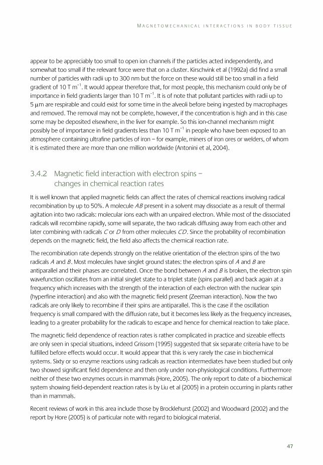
M A G N E T O M E C H A N I C A L I N T E R A C T I O N S I N B O D Y T I S S U E
47
appear to be appreciably too small to open ion channels if the particles acted independently, and somewhat too small if the relevant force were that on a cluster. Kirschvink et al (1992a) did find a small number of particles with radii up to 300 nm but the force on these would still be too small in a field gradient of 10 T m–1. It would appear therefore that, for most people, this mechanism could only be of importance in field gradients larger than 10 T m–1. It is of note that pollutant particles with radii up to 5 μm are respirable and could exist for some time in the alveoli before being ingested by macrophages and removed. The removal may not be complete, however, if the concentration is high and in this case some may be deposited elsewhere, in the liver for example. So this ion-channel mechanism might possibly be of importance in field gradients less than 10 T m–1 in people who have been exposed to an atmosphere containing ultrafine particles of iron – for example, miners of iron ores or welders, of whom it is estimated there are more than one million worldwide (Antonini et al, 2004).
3.4.2 Magnetic field interaction with electron spins – changes in chemical reaction rates
It is well known that applied magnetic fields can affect the rates of chemical reactions involving radical recombination by up to 50%. A molecule AB present in a solvent may dissociate as a result of thermal agitation into two radicals: molecular ions each with an unpaired electron. While most of the dissociated radicals will recombine rapidly, some will separate, the two radicals diffusing away from each other and later combining with radicals C or D from other molecules CD. Since the probability of recombination depends on the magnetic field, the field also affects the chemical reaction rate.
The recombination rate depends strongly on the relative orientation of the electron spins of the two radicals A and B . Most molecules have singlet ground states: the electron spins of A and B are antiparallel and their phases are correlated. Once the bond between A and B is broken, the electron spin wavefunction oscillates from an initial singlet state to a triplet state (spins parallel) and back again at a frequency which increases with the strength of the interaction of each electron with the nuclear spin (hyperfine interaction) and also with the magnetic field present (Zeeman interaction). Now the two radicals are only likely to recombine if their spins are antiparallel. This is the case if the oscillation frequency is small compared with the diffusion rate, but it becomes less likely as the frequency increases, leading to a greater probability for the radicals to escape and hence for chemical reaction to take place.
The magnetic field dependence of reaction rates is rather complicated in practice and sizeable effects are only seen in special situations, indeed Grissom (1995) suggested that six separate criteria have to be fulfilled before effects would occur. It would appear that this is very rarely the case in biochemical systems. Sixty or so enzyme reactions using radicals as reaction intermediates have been studied but only two showed significant field dependence and then only under non-physiological conditions. Furthermore neither of these two enzymes occurs in mammals (Hore, 2005). The only report to date of a biochemical system showing field-dependent reaction rates is by Liu et al (2005) in a protein occurring in plants rather than in mammals.
Recent reviews of work in this area include those by Brocklehurst (2002) and Woodward (2002) and the report by Hore (2005) is of particular note with regard to biological material.
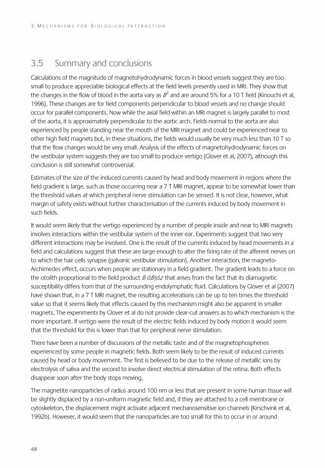
3 M E C H A N I S M S F O R B I O L O G I C A L I N T E R A C T I O N
48
3.5 Summary and conclusions
Calculations of the magnitude of magnetohydrodynamic forces in blood vessels suggest they are too small to produce appreciable biological effects at the field levels presently used in MRI. They show that the changes in the flow of blood in the aorta vary as B 2 and are around 5% for a 10 T field (Kinouchi et al, 1996). These changes are for field components perpendicular to blood vessels and no change should occur for parallel components. Now while the axial field within an MRI magnet is largely parallel to most of the aorta, it is approximately perpendicular to the aortic arch. Fields normal to the aorta are also experienced by people standing near the mouth of the MRI magnet and could be experienced near to other high field magnets but, in these situations, the fields would usually be very much less than 10 T so that the flow changes would be very small. Analysis of the effects of magnetohydrodynamic forces on the vestibular system suggests they are too small to produce vertigo (Glover et al, 2007), although this conclusion is still somewhat controversial.
Estimates of the size of the induced currents caused by head and body movement in regions where the field gradient is large, such as those occurring near a 7 T MRI magnet, appear to be somewhat lower than the threshold values at which peripheral nerve stimulation can be sensed. It is not clear, however, what margin of safety exists without further characterisation of the currents induced by body movement in such fields.
It would seem likely that the vertigo experienced by a number of people inside and near to MRI magnets involves interactions within the vestibular system of the inner ear. Experiments suggest that two very different interactions may be involved. One is the result of the currents induced by head movements in a field and calculations suggest that these are large enough to alter the firing rate of the afferent nerves on to which the hair cells synapse (galvanic vestibular stimulation). Another interaction, the magneto-Archimedes effect, occurs when people are stationary in a field gradient. The gradient leads to a force on the otolith proportional to the field product B dB/dz that arises from the fact that its diamagnetic susceptibility differs from that of the surrounding endolymphatic fluid. Calculations by Glover et al (2007) have shown that, in a 7 T MRI magnet, the resulting accelerations can be up to ten times the threshold value so that it seems likely that effects caused by this mechanism might also be apparent in smaller magnets. The experiments by Glover et al do not provide clear-cut answers as to which mechanism is the more important. If vertigo were the result of the electric fields induced by body motion it would seem that the threshold for this is lower than that for peripheral nerve stimulation.
There have been a number of discussions of the metallic taste and of the magnetophosphenes experienced by some people in magnetic fields. Both seem likely to be the result of induced currents caused by head or body movement. The first is believed to be due to the release of metallic ions by electrolysis of saliva and the second to involve direct electrical stimulation of the retina. Both effects disappear soon after the body stops moving.
The magnetite nanoparticles of radius around 100 nm or less that are present in some human tissue will be slightly displaced by a non-uniform magnetic field and, if they are attached to a cell membrane or cytoskeleton, the displacement might activate adjacent mechanosensitive ion channels (Kirschvink et al, 1992b). However, it would seem that the nanoparticles are too small for this to occur in or around
R E F E R E N C E S
49
magnets that are presently used even when the nanoparticles are strongly coupled with their neighbours in a cluster. This may not be the case, however, in people whose bodies contain micrometre-sized particles of iron as a result of being exposed to an atmosphere containing iron as a pollutant – for example, miners of iron ores or welders.
It is known that magnetic fields can produce appreciable changes in the rates of certain chemical reactions. Considerable effort has been made to see whether these include any biochemical reactions. So far though only one example has been found (Liu et al, 2005) and this involved a protein found in plants but not in mammals.
Acknowledgements
We are grateful to Professor J Dobson and Drs P M Glover and J F Schenck for very helpful discussions.
3.6 References Adrian DJ (1977). Auditory and visual sensations induced by low-frequency electric currents. Radio Sci, 12,
243–50.
Antonini JM, Taylor MD, Zimmer AT and Roberts JR (2004). Pulmonary responses to welding fumes: role of metal constituents. J Toxicol Environ Health, 67, 233–49.
Attwell D (2003). Interaction of low frequency electric fields with the nervous system: the retina as a model system. In: Weak ELF Electric Field Effects in the Body. Proceedings of an International Workshop, March 2003, NRPB, Chilton. Radiat Prot Dosim, 106(4), 341–8.
Barlow HB, Kohn HI and Walsh EG (1947). Visual sensations aroused by magnetic fields. Am J Physiol, 147, 372–5.
Benzanilla F (2000). The voltage sensor in voltage-gated ion channels. Physiol Rev, 80(2), 555–92.
Berry MV and Geim AK (1997). Of flying frogs and levitrons, Eur J Phys, 18, 307–13.
Bourland JD, Nyenhuis JA and Schaefer DJ (1999). Physiologic effects of intense MR imaging gradient fields. Neuroimaging Clin N Am, 9, 363–77.
Brandt T (2003). Vertigo: Its Multisensory Syndromes. New York, Springer.
Brocklehurst B (2002). Magnetic fields and radical reactions: recent developments and their role in nature. Chem Soc Rev, 31, 301–11.
Brody AS, Sorette MP, Gooding CA, Listerud J, Clark MR, Mentzer WC, Brasch RC and James TL (1985). Induced alignment of flowing sickle erythroctes in a magnetic field. A preliminary report. Invest Radiol, 20, 560–66.
Brody AS, Embury SH, Mentzer WC, Winkler ML and Gooding CA (1988). Preservation of sickle call blood-flow patterns during MR imaging: an in vivo study. Am J Roentgenol, 151, 139–41.
Cavin ID, Glover PM, Bowtell RW and Gowland PA (2006). Threshold for perceiving a metallic taste at large magnetic field. 14th Annual Meeting of the International Society for Magnetic Resonance in Medicine, Abstract 2052, Seattle WA, USA.
d’Arsonval A (1896). Disposifs pour las mesure des courants alternatifs de toutes frequencies. Compt Rend Soc Biol, 3, 450–51.
Denegre JM, Valles JM, Jr, Lin K, Jordan WB and Mowry KI (1998). Cleavage planes in frog eggs are altered by strong magnetic fields, Proc Natl Acad Sci USA, 95, 14729–32.
de Vocht F, van Drooge H, Engels, H and Kromhout H (2006a). Exposure, health complaints and cognitive performance among employees of an MRI scanners manufacturing department. J Magn Reson Imaging, 23, 197–204.

3 M E C H A N I S M S F O R B I O L O G I C A L I N T E R A C T I O N
50
de Vocht F, Stevens T, van Wendel-de-Joode B, Engels H and Kromhout H (2006b). Acute neurobehavioral effects of exposure to static magnetic fields: analyses of exposure-response relations. J Magn Reson Imaging, 23, 291–7.
de Vocht F, Stevens T, Glover P, Sunderland A, Gowland P and Kromhout H (2007). Cognitive effects of head-movements in stray fields generated by a 7 tesla whole-body MRI magnet. Bioelectromagnetics, 28(4), 247–55.
Dobson J (2004). Magnetic iron compounds in neurological disorders. Ann NY Acad Sci, 1012, 183–94.
Fitzpatrick RC and Day BL (2004). Probing the human vestibular system with galvanic stimulation. J Appl Physiol, 96, 2301–16.
Gaffey CT and Tenforde TS (1981). Alteration in the rat electrocardiogram induced by stationary magnetic fields, Bioelectromagnetics, 1, 357–70.
Goldberg JM, Smith CE and Fernandez C (1984). Relation between discharge regularity and responses to externally applied galvanic currents in vestibular nerve afferents of the squirrel monkey. J Neurophysiol, 51, 1236–56.
Glover PM, Cavin I, Qian W, Bowtell R and Gowland PA (2007). Magnetic-field-induced vertigo: a theoretical and experimental investigation. Bioelectromagnetics, 28, 349–61.
Grissom CB (1995). Magnetic field effects in biology: a survey of possible mechanisms with emphasis on radical-pair recombination. Chem Rev, 95, 3–24.
Grossman GE, Leigh RJ, Abel LA, Lanska DJ and Thurston SE (1988). Frequency and velocity of rotational head perturbations during locomotion. Exp Brain Res, 70, 470–76.
Hore PJ (2005). Rapporteur’s report: sources and interaction mechanisms. Prog Biophys Mol Biol, 87, 205–12.
Holden AV (2005). The sensitivity of the heart to static magnetic fields. Prog Biophys Mol Biol, 87, 289–320.
Hughes S, El Haj AJ and Dobson J (2005). Med Eng Phys, 27, 754–62.
ICNIRP (2004). Medical magnetic resonance (MR) procedures: protection of patients. Health Phys, 87, 197–216.
Jehenson P, Duboc D, Lavergne T, Guize L, Guerin F, Degeorges M and Syrota A (1988). Change in human cardiac rhythm induced by a 2 T static magnetic field. Radiology, 166(1Part 1), 227–30.
Keltner JR, Roos MS, Brakeman PR and Budinger TF (1990). Magnetohydrodynamics of blood flow. Magn Reson Med, 16(1), 139–49.
Kinouchi Y, Yamaguchi H and Tenforde TS (1996). Theoretical analysis of magnetic field interactions with aortic blood flow. Bioelectromagnetics, 17, 21–32.
Kirschvink JL, Kobayaschi-Kirschvink A and Woodford BJ (1992a). Magnetite biomineralization in the human brain. Proc Nat Acad Sci USA, 89, 7683–7.
Kirschvink JL, Kobayaschi-Kirschvink A, Diaz-Ricci JC and Kirschvink SJ (1992b). Magnetite in human tissues: a mechanism for the biological effects of weak ELF magnetic fields. Bioelectromagnetics, Suppl 1, 101–13.
Kornhuber HH (1974). In: Vestibular System (HH Kornhuber, ed). Berlin, Springer-Verlag.
Liu F, Zhao H and Crozier S (2003). Calculation of electric fields induced by body and head motion in high-field MRI. J Magn Reson, 161, 99–107.
Liu Y, Edge R, Timmel CR, Henbest K, Hore PJ and Gast P (2005). Magnetic field effect on singlet oxygen production in a biochemical system. Chem Commun (Camb), 2, 174–6.
Lövsund P, Öberg A, Nilsson SEG and Reuter T (1980). Magnetophosphenes: a quantitative analysis of thresholds. Med Biol Eng Comput, 18, 326–34.
Luxon L (2006). Personal communication. University College London (UCL).
McCormick DA (1998). Membrane properties and neurotransmitter actions. In: The Synaptic Organisation of the Brain (GM Shepherd, ed). Oxford University Press, pp 37–76.
MacDougall HG and Moore S (2005). Marching to the beat of the same drummer: the spontaneous tempo of human locomotion. J Appl Physiol, 99, 1164–73.
Murayama M (1965). Orientation of sickled eryothrocytes in a magnetic field, Nature, 206, 420–22.
Murayama M (1966). Molecular mechanism of red cell ‘sickling’. Science, 153, 145–9.
Murayama M, Olson RA and Jennings WH (1966). Molecular orientation in horse hemoglobin crystals and sickled eryothrocytes Biochim Biophys Acta, 94, 194–9.
R E F E R E N C E S
51
Noble D and Stein RB (1966). The threshold conditions for initiation of action potentials by excitable cells. J Physiol, 187, 129–62.
Nyenhuis JA, Bourland JD, Kildishev AV and Schaefer DJ (2001). Health effects and safety of intense gradient fields. In Magnetic Resonance Procedures: Health Effects and Safety (FD Shellock, ed). New York, CRC Press, pp 31–53.
Oman CM and Young LR (1972). The physiological range of pressure difference and cupula deflections in the human semicircular canal. Theoretical considerations. Acta Otolaryngol, 74(5), 324–31.
Oshitani J, Yamada D, Miyahara M and Higashitani K (1999). Magnetic effect on ion-exchange kinetics. J Colloid Interface Sci, 210, 1–7.
Otsuka S (1988). Introduction. In: Metalloproteins: Chemical Properties and Biological Effects (S Otsuka and T Yamanaka, eds). Tokyo, Kodansha.
Pozzo T, Berthoz A and Lefort L (1990). Head stabilisation during various locomotor tasks in humans. Exp Brain Res, 82, 97–106.
Rabbitt RD, Yamauchi AM, Boyle R and Highstein SM (2001). How endolymph pressure modulates semicircular canal primary afferent discharge. Ann NY Acad Sci, 942, 313–21.
Reilly JP (1998). Stimulation via electric and magnetic fields. In: Applied Bioelectricity: from Electrical Stimulation to Electropathology (JP Reilly, ed). New York, Springer, Chapter 9, pp 341–411.
Saunders RD and Jefferys JGR (2002). Weak electric field interactions in the central nervous system. Health Phys, 83(3), 366–75.
Schenck JF (1992a). Health and physiological effects of human exposure to whole-body four-tesla magnetic fields during MRI. Ann NY Acad Sci, 649, 285–301.
Schenck JF (1992b). Quantitative assessment of the magnetic forces and torques on red blood cells: implications for patients with sickle cell anemia. In: Society of Magnetic Resonance in Medicine, 11th Annual Meeting, Berlin, p 3405.
Schenck JF (2005). Physical interactions of static magnetic fields with living tissues. Prog Biophys Mol Biol, 87, 185–204.
Schenck JF (2006). Personal communication. General Electric Global Research Center, Schenectady, New York.
Stephan T, Deutschländer A, Nolte A, Schneider E, Wiesmann M, Brandt T and Dieterich M (2005). Functional MRI of galvanic vestibular stimulation with alternating currents at different frequencies. Neuroimage, 26, 721–32.
Tenforde TS, Gaffey CT, Moyer BR and Budinger TF (1983). Cardiovascular alterations in Macaca monkeys exposed to stationary magnetic fields: experimental observations and theoretical analysis. Bioelectromagnetics, 4, 1–9.
Togawa T, Okai O and Oshima M (1967). Observation of blood flow EMF in externally applied strong magnetic field by surface electrodes. Med Biol Eng Comput, 5, 169–70.
Valles JM, Jr, Lin K, Denegre JM and Mowry KL (1997). Stable magnetic field gradient levitation of Xenopus laevis toward low-gravity simulation. Biophys J, 73, 1130–33.
Valles JM, Jr, Wasserman SR, Schweidenback C, Edwardson J, Denegre JM and Mowry KL (2002). Processes that occur before second cleavage determine third cleavage orientation in Xenopus. Exp Cell Res, 274, 112–18.
Valles JM, Jr, and Guevorkian K (2002). Low gravity on earth by magnetic levitation of biological material. J Gravit Physiol, 9, 11–14.
Watson SR and Colebatch JG (1998). Vestibulocollic reflexes evoked by short-duration galvanic stimulation in man. J Physiol, 513, 587–97.
Woodward JR (2002). Radical pairs in solution. Prog React Kinet Mech, 27, 165–207.
52
4 Cellular Studies
Cellular studies are useful in the assessment of the potential effect of various chemical and physical agents on biological systems. They have the advantages over human and animal studies that the procedures are relatively quick and inexpensive so many experiments can be undertaken to test a variety of agents in a wide selection of isolated cell types, and the test conditions can be well defined and controlled in a way that would be difficult to achieve in studies of animals or humans. Cellular studies can be used as a screening process to eliminate or highlight areas of interest and concern. They can also indicate possible mechanisms involved in the interactions of physical or chemical agents with cells. The disadvantage is that any effect found is a cellular response, may not be paralleled by similar changes in whole organisms, and therefore cannot necessarily be extrapolated directly to a health effect.
Cellular studies investigating the effects of static magnetic fields have covered a wide range of biological systems, from bacteria and fungi, through seeds and plants, to animal and human cells. The magnetic flux densities have also covered a broad range, but generally have tended to be high in comparison with the geomagnetic field, typically several tens of millitesla. Few studies in the millitesla range have indicated possible harmful effects. In general, there is a poor record of reproducibility of findings at lower magnetic flux densities, and even the effects that have been reported do not appear to form a consistent or cohesive pattern in terms of exposure parameters or biological response. Given the unsupported and conflicting nature of the findings at lower magnetic flux densities, little can be concluded from these studies. Consequently the review of studies in this chapter has been limited to those using stronger fields, typically greater than 0.2 T. A review of some studies carried out with fields below 0.2 T has been carried out by the World Health Organization (WHO, 2006).
4.1 Genotoxic effects
4.1.1 Mutation studies
Mutation studies of bacteria are a rapid way to assess the potential genotoxicity of chemical or physical agents.
The possible genotoxic effect of static magnetic fields has been studied in several bacterial strains (Ikehata et al, 1999). No mutagenic response was seen in various strains of Salmonella typhimurium (TA98, TA100, TA1535 and TA1537) and Escherichia coli (WP2 uvrA) when exposed to fields of up to 5 T for 1.5 to 24 hours. However, when the E coli were tested with one of ten chemical mutagens simultaneously with either 2 or 5 T magnetic fields, some chemicals (N-ethyl-N ’-nitro-N-nitrosoguanidine, N-methyl-N ’-nitro-N-nitrosoguanidine, ethylmethanesulphonate, 4-nitroquinoline-N-oxide, 2-amino-3-methyl-3H-imidazow[4,5-f]quinoline and 2-(2-furyl)-3-(5-nitro-2-furyl) acrylamide) showed a synergistic effect with the magnetic field so that the mutation rate increased significantly above that for chemical mutagen alone.

G E N O T O X I C E F F E C T S
53
No mutagenic effect was found (using the Ames test) in tested bacterial strains of E coli when exposure took place in a diagnostic 1.5 T MRI scanner or at 7.2 T. Furthermore there was no difference from control when exposure was to gradient or high frequency fields, nor was there a synergistic effect when magnetic field exposure was combined with known genotoxic chemicals (Teichmann et al, 2000).
Similarly, no effect on E coli mutation was seen (Zhang et al, 2003) in wild-type (strain GC4468) bacteria or mutants defective in DNA repair after exposure of up to 9 T for 24 hours. However, mutant strains that were defective in defence mechanisms against oxidative stress had significantly increased rates of mutation.
4.1.2 Chromosomal damage
Effects of 0.5 and 1.0 T magnetic fields on human blood cells were investigated (Cooke and Morris, 1981) to look for the frequency of gross lesions and sister chromatid exchange. No statistically significant effects were found after one hour of exposure.
The effects of stronger fields were tested (Okonogi et al, 1996) when using mitomycin C to induce micronucleus formation in Chinese hamster lung (CHL/IU) cells, a standard cell line for tests of chromosomal aberration. Simultaneous exposure to 4.7 T magnetic fields for six hours reduced the number of induced micronuclei. The time course for the appearance of the maximum number of micronuclei was the same with or without the magnetic field. The authors suggested that the magnetic field might have had a protective effect at the stage of induction of DNA damage by mitomycin C rather than on formation of the micronuclei.
Exposure to static magnetic fields up to 10 T had no effect on cell growth, cell cycle distribution and micronucleus formation in Chinese hamster ovary cells exposed for up to four days (Nakahara et al, 2002). However, micronuclei induced by exposure of the cells to X-rays (4 Gy) were significantly increased by 10 T static fields but not by 1 T fields.
4.1.3 DNA damage
Various mutant strains of E coli were exposed for up to 24 hours to a homogeneous static magnetic field of either 0.5 or 3.0 T (Mahdi et al, 1994). No evidence of increased DNA damage was detected, even in bacterial strains that had a defective DNA repair mechanism. In contrast, ten seconds of exposure to ultraviolet radiation (1 W m–2) severely compromised survival in the most sensitive bacterial strain.
After exposure to 6.34 T magnetic fields for 24 hours, human colon carcinoma cells (HCT116) that were deficient in DNA mismatch repair and repair proficient human cervical adenocarcinoma (HeLa S3) cells exhibited no significant effect on microsatellite changes (Okuda et al, 1998). Cells that lack DNA mismatch repair are unable to correct errors during DNA replication. Microsatellites (non-coding repeat sequences of DNA) are susceptible to change and are therefore sensitive regions of DNA for detection of these errors. In contrast to magnetic fields, irradiation by low dose X-rays (2 Gy) significantly increased microsatellite changes in cells deficient in mismatch repair.
4 C E L L U L A R S T U D I E S
54
4.1.4 Proliferation
Factors that affect proliferation potentially have a role in carcinogenesis. Human gingival fibroblasts in confluent cultures were continuously exposed to a 0.2 T static magnetic field for six or eight months. However, no effect of exposure was found in the rate of cell proliferation, DNA content, metabolic rate or cell morphology (Yamaguchi et al, 1993).
A magnetic field of 0.2 T was also used to expose normal human neuronal cell cultures (FNC-B4), although for a much shorter period of 15 minutes (Pacini et al, 1999b). This produced changes in morphology and reduced thymidine incorporation, indicating decreased DNA synthesis and hence inhibition of proliferation. However, analysis of 12 DNA microsatellites selected as indicators of genome instability revealed no alteration following exposure, thus ruling out a direct effect of the magnetic field on DNA stability. Interestingly, non-neuronal cells (mouse leukaemia and human breast carcinoma cells) showed no alteration following exposure, although when human breast carcinoma cells were treated with vitamin D the exposure to magnetic fields slowed cell growth (Pacini et al, 1999a). In a later study (Pacini et al, 2003) human skin fibroblasts exposed to 0.2 T for one hour had modified cell morphology and decreased thymidine incorporation.
Differences in response to magnetic field exposure (0.5 T for six days) were also seen between African green monkey renal cells (VERO) and rat astrocytes (Buemi et al, 2001). The renal cells had decreased apoptosis and proliferation, whereas the astrocytes showed an increase in the same parameters.
The effect of repetitive exposure to a static magnetic field of 1.5 T on the proliferation of human fetal lung fibroblasts was assessed by exposing the cells for one hour three times a week for three weeks (Wiskirchen et al, 1999). DNA synthesis, cell cycle and proliferation were not altered by magnetic field exposure. A further study (Wiskirchen et al, 2000) extended the range of exposure conditions to 0.2, 1.0 and 1.5 T for one hour each day for five consecutive days applied to synchronised and non-synchronised cells. No effect on cell growth and cell cycle distribution was detected.
Similarly, no effect was found on cell growth in isolated human peripheral lymphocytes when exposed to magnetic fields up to 6.3 T for three days. Magnetic fields of up to 2 T in combination with phytohaemaglutinin (PHA) stimulated cell proliferation but no greater than by PHA alone. However, exposure to fields greater than 4 T caused inhibition of growth in cells stimulated by PHA (Norimura et al, 1993). The need for cells to be proliferating for an effect of magnetic fields to be observed was supported in another study (Onodera et al, 2003) in which peripheral blood mononuclear cells showed no change in growth with fields of up to 10 T for four hours, but when the cells were stimulated by PHA the addition of a magnetic field caused a decrease in cell number and an increase in cell death compared with PHA alone.
Human peripheral blood mononuclear cells exposed to a 4.75 T field for one hour with or without activation by phytohaemaglutinin showed no proliferative, activating or pro-inflammatory effects (Aldinucci et al, 2003b). Also, the concentration of interleukin-1beta, interleukin-2, interleukin-6, interferon and tumour necrosis factor alpha remained unchanged in exposed cells. In contrast, exposure of Jurkat cells statistically decreased the proliferation and halved the intracellular calcium concentration. The authors suggested that the static magnetic field changed the properties of the cell membrane in

G E N O T O X I C E F F E C T S
55
Jurkat cells, which in turn influenced calcium ion transport processes, and calcium ion homeostasis. A further study (Aldinucci et al, 2003a) showed increased intracellular calcium in normal and activated lymphocytes, but this was not translated into an activating or pro-inflammatory effect.
Exposure to a static magnetic field of 1 T in combination with radiofrequency (RF) radiation of the type used in NMR equipment had no effect on cell death in blood mononuclear cells but doubled the rate of cell-damage-induced death in human tumour cells (U937) and Jurkat cells due to elevated calcium ion levels caused by uncontrolled influx (Ghibelli et al, 2006). Agents that blocked the effect of calcium ion influx protected the tumour cells from exposure-induced damage, indicating that calcium ions play an important role in the cellular effects of magnetic fields.
Three malignant human cell lines, HTB 63 (melanoma), HTB 77 IP3 (ovarian carcinoma), and CCL 86 (lymphoma: Raji cells), were exposed to a 7 T magnetic field for 64 hours. Exposure reduced the number of viable cells in each cell line by 20% to 40%; however, the cell cycle was unaltered and there was no increase in DNA breaks (Raylman et al, 1996).
Two tumour cell lines, human promyelocyte leukaemia (HL60) and mouse lymphoma (EA2), were exposed to static magnetic fields of 1.5 and 7 T for periods between 1 and 24 hours (Schiffer et al, 2003). Cell cycle analysis revealed no differences due to the magnetic field exposure, whereas the positive controls that were gamma irradiated (8 Gy) showed an arrest in the cell cycle at G2/M.
No difference in cell growth was found in mouse leukaemia cells (P388) and Chinese hamster fibroblasts (V79) when exposed to 7 T magnetic fields for 3 or 24 hours. Furthermore, exposure in the presence of the antitumour agent bleomycin had no additional effect (Sakurai et al, 1999).
DNA synthesis and cell survival were examined in Chinese hamster (V79) cells with and without fast-neutron irradiation. Several hours of magnetic field exposure at 0.75 T alone showed no effect. The detrimental effects caused by fast-neutron irradiation were not increased by magnetic field exposure applied during or after irradiation (Ngo et al, 1987).
The effects of spatial magnetic field gradients have been investigated (Sato et al, 1992). There was no change in the growth of HeLa cells and isolated human gingival fibroblasts when exposed for up to 48 hours to an inhomogeneous magnetic field that was more than 1.5 T at the centre of the dish and decreased rapidly with distance from the centre.
One study has looked at the effect of static magnetic fields on micro-organisms in the human body. The growth kinetics of E coli in simulated human intestinal conditions did not change when the bacteria were exposed to a 0.45 T static magnetic field (Arisawa et al, 1996).
No effect on the growth of yeast (Saccharomyces cerevisiae) was seen over seven cell divisions when exposed to 1.5 T magnetic fields (Malko et al, 1994). However, with exposure to stronger fields of 9–14 T with a maximum flux density gradient, dB/dz, of 94 T m−1, a decreased rate of proliferation was observed (Iwasaka et al, 2004). Under the exposure conditions of a gradient magnetic field the liquid surface was observed to incline due to the diamagnetism of water. In addition, migration of the yeast cells in the solution under the influence of the applied magnetic field caused changes in the sedimentation pattern of the yeast.
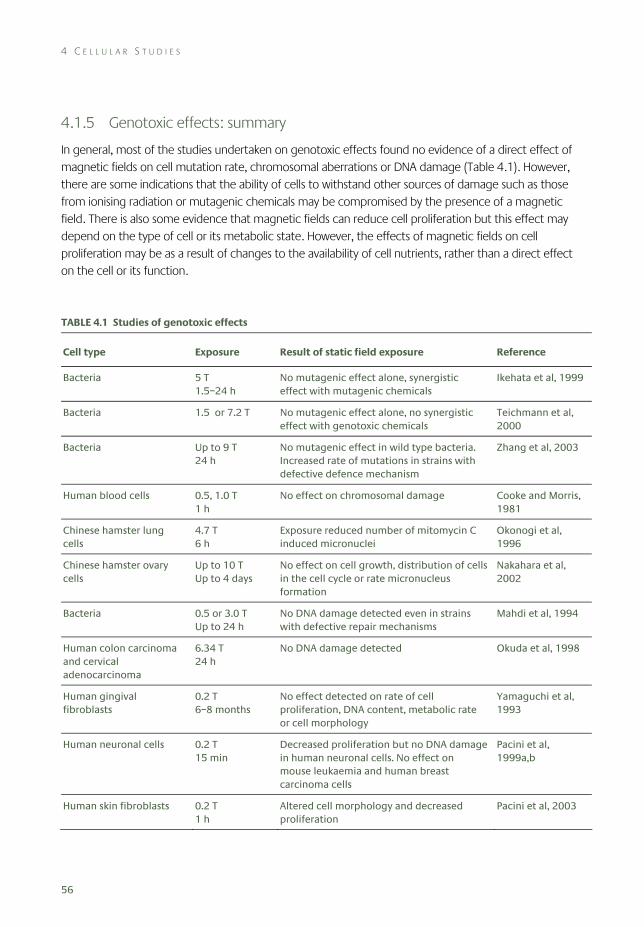
4 C E L L U L A R S T U D I E S
56
4.1.5 Genotoxic effects: summary
In general, most of the studies undertaken on genotoxic effects found no evidence of a direct effect of magnetic fields on cell mutation rate, chromosomal aberrations or DNA damage (Table 4.1). However, there are some indications that the ability of cells to withstand other sources of damage such as those from ionising radiation or mutagenic chemicals may be compromised by the presence of a magnetic field. There is also some evidence that magnetic fields can reduce cell proliferation but this effect may depend on the type of cell or its metabolic state. However, the effects of magnetic fields on cell proliferation may be as a result of changes to the availability of cell nutrients, rather than a direct effect on the cell or its function.
TABLE 4.1 Studies of genotoxic effects
Cell type Exposure Result of static field exposure Reference
Bacteria 5 T 1.5–24 h
No mutagenic effect alone, synergistic effect with mutagenic chemicals
Ikehata et al, 1999
Bacteria 1.5 or 7.2 T No mutagenic effect alone, no synergistic effect with genotoxic chemicals
Teichmann et al, 2000
Bacteria Up to 9 T 24 h
No mutagenic effect in wild type bacteria. Increased rate of mutations in strains with defective defence mechanism
Zhang et al, 2003
Human blood cells 0.5, 1.0 T 1 h
No effect on chromosomal damage Cooke and Morris, 1981
Chinese hamster lung cells
4.7 T 6 h
Exposure reduced number of mitomycin C induced micronuclei
Okonogi et al, 1996
Chinese hamster ovary cells
Up to 10 T Up to 4 days
No effect on cell growth, distribution of cells in the cell cycle or rate micronucleus formation
Nakahara et al, 2002
Bacteria 0.5 or 3.0 T Up to 24 h
No DNA damage detected even in strains with defective repair mechanisms
Mahdi et al, 1994
Human colon carcinoma and cervical adenocarcinoma
6.34 T 24 h
No DNA damage detected Okuda et al, 1998
Human gingival fibroblasts
0.2 T 6–8 months
No effect detected on rate of cell proliferation, DNA content, metabolic rate or cell morphology
Yamaguchi et al, 1993
Human neuronal cells 0.2 T 15 min
Decreased proliferation but no DNA damage in human neuronal cells. No effect on mouse leukaemia and human breast carcinoma cells
Pacini et al, 1999a,b
Human skin fibroblasts 0.2 T 1 h
Altered cell morphology and decreased proliferation
Pacini et al, 2003
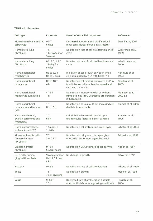
G E N O T O X I C E F F E C T S
57
TABLE 4.1 Continued
Cell type Exposure Result of static field exposure Reference
Monkey renal cells and rat astrocytes
0.5 T 6 days
Decreased apoptosis and proliferation in renal cells; increase found in astrocytes
Buemi et al, 2001
Human fetal lung fibroblasts
1.5 T 1 h, 3/week for 3 weeks
No effect on rate of cell proliferation or cell cycle
Wiskirchen et al, 1999
Human fetal lung fibroblasts
0.2, 1.0, 1.5 T 1 h/day for 5 days
No effect on rate of cell proliferation or cell cycle
Wiskirchen et al, 2000
Human peripheral lymphocytes
Up to 6.3 T Up to 3 days
Inhibition of cell growth only seen when cells stimulated by PHA with fields >4 T
Norimura et al, 1993
Human peripheral monocytes
Up to 10 T 4 h
No effect on cells unless stimulated by PHA in which case cell number decreased and cell death increased
Onodera et al, 2003
Human peripheral monocytes, Jurkat cells
4.75 T 1 h
No effect on monocytes with or without stimulation by PHA. Decreased proliferation in Jurkat cells
Aldinucci et al, 2003a,b
Human peripheral monocytes and tumour cells
1 T Up to 5 h
No effect on normal cells but increased cell death in tumour cells
Ghibelli et al, 2006
Human melanoma, ovarian carcinoma and lymphoma
7 T 64 h
Cell viability decreased, but cell cycle unaltered, no increase in DNA damage
Raylman et al, 1996
Human promyelocyte leukaemia and EA2
1.5 and 7 T 1–24 h
No effect on cell distribution in cell cycle Schiffer et al, 2003
Mouse leukaemia cells, Chinese hamster fibroblasts
7 T 3 or 24 h
No effect on cell growth; no synergistic effect with antitumour agent beomycin
Sakurai et al, 1999
Chinese hamster fibroblasts
0.75 T Several hours
No effect on DNA synthesis or cell survival Ngo et al, 1987
HeLa cells, human gingival fibroblasts
Strong gradient field 1.5 T max 48 h
No change in growth Sato et al, 1992
Bacteria 0.45 T No effect on rate of cell proliferation Arisawa et al, 1996
Yeast 1.5 T 7 cell divisions
No effect on growth Malko et al, 1994
Yeast 9–14 T 16 h
Decreased rate of proliferation but field affected the laboratory growing conditions
Iwasaka et al, 2004

4 C E L L U L A R S T U D I E S
58
4.2 Changes in cellular processes
4.2.1 Gene expression
Gene expression of yeast (S cerevisiae) was not altered by exposure to 5 T static magnetic fields for 2 hours, although the sedimentation pattern of the yeast was changed. Nor did exposure to 10 T for 1 hour or 5 T for 24 hours affect gene expression. However, a slight change in expression of several genes that are related to respiration was observed with exposure to a 14 T static magnetic field for 24 hours (Ikehata et al, 2003).
Human promyelocyte leukaemia (HL60) cells exposed for periods of 1 to 48 hours to either a 6 T field with a magnetic flux density gradient of 41.7 T m−1 or a spatially homogeneous 10 T static magnetic field showed no differences in levels of c-Myc and c-Fos protein expression. In contrast, c-Jun protein expression increased at all time points up to 72 hours in HL60 cells after exposure to a 6 T field with a gradient but was not altered by a homogeneous 10 T field (Hirose et al, 2003b).
Human peripheral blood mononuclear cells from healthy volunteers exposed for two hours at 24°C to 0.5 T static magnetic fields had decreased expression of an early T-cell activation antigen (CD69), which is involved in lymphocyte proliferation. However, the cells had increased release of interferon-gamma and interleukin-4, which are linked to regulation of the immune response (Salerno et al, 1999).
4.2.2 Intracellular signalling
A cellulose membrane exposed to a static magnetic field of 0.24 T had a significantly enhanced rate of potassium ion transport which did not return to the initial basal level after exchange of the aqueous medium (Ohata et al, 2004). The results suggest that an irreversible change took place on the cellulose membrane or on the water bound to the cellulose surface. The authors suggested that the increased rate of ion transport may have occurred as a result of a stabilised hydration layer on the cellulose surface.
Exposure of the fungus Fusarium culmorum to a static magnetic field of 0.3 T inhibited mycelia growth and was accompanied by morphological and biochemical changes. Germination of asexual fungal spores and cell viability were also reduced. The effects appeared to be through calcium-dependent signal transduction pathways. Perturbation of these pathways by adding different compounds (ie calcium chloride, phorbol 12-myristate 13-acetate, neomycin, EGTA or lithium chloride) to the medium, suggested that exposed asexual spores were unable to mobilise calcium from intracellular stores (Albertini et al, 2003).
C H A N G E S I N C E L L U L A R P R O C E S S E S
59
4.2.3 Metabolic activity
Exposure of glandular tissue from breast cancers and from healthy women to a 0.2 T magnetic field showed that cancer tissue had a greater sensitivity to dehydration compared with normal tissue (Danielyan et al, 1999).
Metabolic activity was reduced by 20% in HL60 cells exposed to a 1 T static magnetic field for 72 hours. Additionally, the magnetic exposure enhanced the cytotoxic effect of antineoplastic drugs (5-fluorouracil, cisplatin, doxorubicin and vincristine) on these cells (Sabo et al, 2002).
Continuous 0.4 T static fields applied to bone-forming osteoblast-like cells (MG63) for periods up to 72 hours caused the cells to have a more differentiated appearance due to local increased production of regulatory factors (Huang et al, 2006).
4.2.4 Aggregation and cell adhesion
Changes in sedimentation patterns have been seen in studies on erythrocytes (Iino, 1997). The erythrocyte sedimentation rate in saline measured by the Westergren method was slightly increased by a 6.3 T static magnetic field applied in a vertical direction. However, the rate was greatly enhanced when plasma was used instead of saline. This was explained by an increase in cell aggregation and hence an increased sedimentation rate. A further study (Iino and Okuda, 2001) showed that the aggregation was due to a magnetic-field-induced increase in intermembrane adhesion dependent on the orientation of the erythrocytes.
Not all cells show increased aggregation in magnetic fields. Melanophores, black pigment cells from the fins of tetra fish, had an unaltered pattern of aggregation when exposed to 8 or 14 T fields (Testorf et al, 2002).
A study into the adherence of cells to the tissue culture surface (Short et al, 1992) showed that a 4.7 T magnetic field impaired the adhesion of malignant melanoma cells but not normal human fibroblasts. Cell proliferation and viability were not affected.
4.2.5 Changes in cellular processes: summary
Only a few studies have investigated changes in gene expression in relation to exposure to static magnetic fields greater than 0.2 T (Table 4.2). The studies used relatively long exposures but differed in flux density and biological endpoints. Nonetheless they all found some, albeit in one case slight, effects. Similarly, the studies of intracellular signalling all found changes in the various cells that were investigated. The changes were mainly increased intracellular calcium ion concentration. As with the cell proliferation studies, there is some suggestion that the effects are the result of magnetic-field-induced changes to the growth media surrounding the cells, rather than a direct effect on the cells. There is some evidence that cell adhesion, either cell to cell or cell to plastic, can be affected by static magnetic field exposure, but there may be differences in response between types of cell.
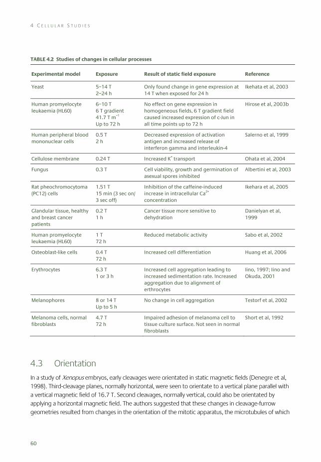
4 C E L L U L A R S T U D I E S
60
TABLE 4.2 Studies of changes in cellular processes
Experimental model Exposure Result of static field exposure Reference
Yeast 5–14 T 2–24 h
Only found change in gene expression at 14 T when exposed for 24 h
Ikehata et al, 2003
Human promyelocyte leukaemia (HL60)
6–10 T 6 T gradient 41.7 T m–1 Up to 72 h
No effect on gene expression in homogeneous fields, 6 T gradient field caused increased expression of c-Jun in all time points up to 72 h
Hirose et al, 2003b
Human peripheral blood mononuclear cells
0.5 T 2 h
Decreased expression of activation antigen and increased release of interferon gamma and interleukin-4
Salerno et al, 1999
Cellulose membrane 0.24 T Increased K+ transport Ohata et al, 2004
Fungus 0.3 T Cell viability, growth and germination of asexual spores inhibited
Albertini et al, 2003
Rat pheochromocytoma (PC12) cells
1.51 T 15 min (3 sec on/ 3 sec off)
Inhibition of the caffeine-induced increase in intracellular Ca2+ concentration
Ikehara et al, 2005
Glandular tissue, healthy and breast cancer patients
0.2 T 1 h
Cancer tissue more sensitive to dehydration
Danielyan et al, 1999
Human promyelocyte leukaemia (HL60)
1 T 72 h
Reduced metabolic activity Sabo et al, 2002
Osteoblast-like cells 0.4 T 72 h
Increased cell differentiation Huang et al, 2006
Erythrocytes 6.3 T 1 or 3 h
Increased cell aggregation leading to increased sedimentation rate. Increased aggregation due to alignment of erthrocytes
Iino, 1997; Iino and Okuda, 2001
Melanophores 8 or 14 T Up to 5 h
No change in cell aggregation Testorf et al, 2002
Melanoma cells, normal fibroblasts
4.7 T 72 h
Impaired adhesion of melanoma cell to tissue culture surface. Not seen in normal fibroblasts
Short et al, 1992
4.3 Orientation
In a study of Xenopus embryos, early cleavages were orientated in static magnetic fields (Denegre et al, 1998). Third-cleavage planes, normally horizontal, were seen to orientate to a vertical plane parallel with a vertical magnetic field of 16.7 T. Second cleavages, normally vertical, could also be orientated by applying a horizontal magnetic field. The authors suggested that these changes in cleavage-furrow geometries resulted from changes in the orientation of the mitotic apparatus, the microtubules of which
O R I E N T A T I O N
61
were acted on directly by the magnetic field. In similar experiments a change in the direction of the third cleavage plane was also seen at 8 T (Eguchi et al, 2006), although this effect was overcome by rotating the embryos continually in the magnetic field. Despite these changes to early cleavage direction in embryos exposed to static magnetic fields, the embryos in the latter study all developed into normal tadpoles.
In another study, bull sperm, which has a very flat head, was orientated with the whole body and the head perpendicular to the direction of a 1 T static magnetic field (Emura et al, 2001). The diamagnetic cell components, such as the cell membrane, the DNA in the head, and the microtubule in the tail, were suggested to contribute to this orientation. The authors noted that the magnetic orientation was very strong in comparison with that of erythrocytes or platelets.
Perpendicular orientation of sickle erythrocytes to a 0.35 T static magnetic field was reported by Murayama (1965). A similar effect was seen in deoxygenated sickle erythrocytes (Brody et al, 1985) using a 0.38 T field.
However, normal erythrocytes were orientated with their disk plane parallel to the magnetic field direction; this influence was seen at 1 T and almost all of the cells were orientated when exposed to 4 T. Furthermore, the degree of orientation was not influenced by the state of haemoglobin (oxy: diamagnetic, deoxy and met: paramagnetic). The dependence of the measured degree of orientation on the intensity of the magnetic field was in good agreement with the theoretical equation for the magnetic orientation of diamagnetic constituents of the membrane (Higashi et al, 1993). In contrast, a later study using glutaraldehyde-fixed erythrocytes showed an orientation in which their disk plane was perpendicular to an 8 T magnetic field. The paramagnetism of membrane-bound haemoglobin was thought to contribute significantly to this orientation (Higashi et al, 1996).
After 60 hours of exposure to static magnetic fields, cultured mouse osteoblast (MC3T3-E1) cells were transformed to rod-like shapes and were orientated in a direction parallel to the 8 T magnetic fields. The exposure did not affect cell proliferation, but did increase cell differentiation and matrix synthesis (Kotani et al, 2002).
Orientation of human glioblastoma (A172) cells following exposure to static magnetic fields at 10 T in the presence or absence of collagen showed that cells embedded in collagen gel were orientated perpendicular to the direction of the magnetic field. Cells cultured in the absence of collagen exhibited no specific orientation pattern after seven days of exposure. The results suggest that the orientation of glioblastoma cell processes may be due to the arrangement of microtubules under the influence of magnetically orientated collagen fibres (Hirose et al, 2003a).
After 60 hours of exposure to an 8 T magnetic field Schwann cells orientated parallel to the magnetic fields. In contrast, Schwann cells orientated in the direction perpendicular to the magnetic field after two hours of magnetic field exposure when collagen was present. The Schwann cells aligned along the collagen fibres orientated by the magnetic fields (Eguchi et al, 2003).
Human foreskin fibroblasts cultured in a collagen gel were orientated as a result of collagen fibre alignment in 4 T magnetic fields (Guido and Tranquillo, 1993).
4 C E L L U L A R S T U D I E S
62
To investigate the relationship between magnetic cell orientation and factors such as cell type and cell density, A7r5 cells (smooth muscle cell, spindle shaped), GI-1 cells (human glioma, spindle shaped), and HEK293 cells (human kidney cell, polygonal shaped) were exposed to an 8 T static magnetic field for 60 hours at 37°C (Ogiue-Ikeda and Ueno, 2004). The spindle shaped cells were orientated by the magnetic field; however, polygonal shaped cells were not. A7r5 cells were orientated by the magnetic field only when the cells were actively proliferating at high cell density; when the cells were in the confluent condition at the start of magnetic field exposure, the cells were not subsequently orientated. The authors concluded that the magnetic field affected the cell division process, and only the proliferating cells at high density were orientated under the magnetic field.
Smooth muscle cells of a rat were cultured in a Petri dish and observed microscopically in magnetic fields of up to 14 T. The findings indicated that the intracellular cyto-skeleton proteins rotated within three hours of exposure due to the diamagnetic torque acting on them (Iwasaka and Ueno, 2002). In a further study the magnetic field was shown to influence the shape of the cell colonies by causing them to extend along the direction of the magnetic flux. The phenomenon was most notable under magnetic fields of more than 10 T, where an ellipsoidal pattern of smooth muscle cell colonies was observed. The authors speculated that the mechanism was a diamagnetic torque acting on cytoskeleton fibres, which were dynamically polymerising and depolymerising during cell division and cell migration (Iwasaka et al, 2003). Within an exposure period of three days, such magnetic fields generated an alignment of the smooth muscle cell assembly, which was parallel to the direction of the fields.
Self-assembly of collagen fibrils from a solution orientated the fibrils into planes normal to the direction of a 1.9 T magnetic field. However, skeletal muscle actin orientated parallel to a 7 T field (Torbet and Dickens, 1984; Torbet and Ronziere, 1984).
Some long-chain phospholipid bilayers have been shown to align spontaneously in a static magnetic field. The alignment could be altered by the chemical composition: the perpendicular alignment of the phospholipid bilayer could be made parallel to a 7 T magnetic field by the inclusion of paramagnetic lanthanide ions (Tiburu et al, 2001).
4.3.1 Orientation: summary
There have been several studies devoted to the phenomena of macromolecular or cellular orientation in a magnetic field (Table 4.3). Macromolecules, such as collagen and actin, have been shown to orientate in a magnetic field, although the direction of orientation is dependent on the particular macromolecule. Most studies have used relatively strong magnetic fields, typically 8 T or more. However, even relatively modest fields (around 0.35 T) are claimed to orientate some cells. When cells orientate they tend to do so parallel to the direction of the magnetic field. However, there appear to be some exceptions – for instance, sickle erythrocytes, bull sperm or where the orientation is determined by the presence of external macromolecules such as collagen.
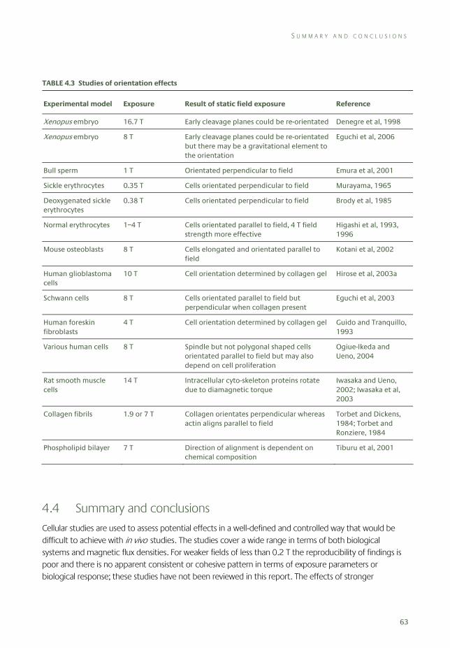
S U M M A R Y A N D C O N C L U S I O N S
63
TABLE 4.3 Studies of orientation effects
Experimental model Exposure Result of static field exposure Reference
Xenopus embryo 16.7 T Early cleavage planes could be re-orientated Denegre et al, 1998
Xenopus embryo 8 T Early cleavage planes could be re-orientated but there may be a gravitational element to the orientation
Eguchi et al, 2006
Bull sperm 1 T Orientated perpendicular to field Emura et al, 2001
Sickle erythrocytes 0.35 T Cells orientated perpendicular to field Murayama, 1965
Deoxygenated sickle erythrocytes
0.38 T Cells orientated perpendicular to field Brody et al, 1985
Normal erythrocytes 1–4 T Cells orientated parallel to field, 4 T field strength more effective
Higashi et al, 1993, 1996
Mouse osteoblasts 8 T Cells elongated and orientated parallel to field
Kotani et al, 2002
Human glioblastoma cells
10 T Cell orientation determined by collagen gel Hirose et al, 2003a
Schwann cells 8 T Cells orientated parallel to field but perpendicular when collagen present
Eguchi et al, 2003
Human foreskin fibroblasts
4 T Cell orientation determined by collagen gel Guido and Tranquillo, 1993
Various human cells 8 T Spindle but not polygonal shaped cells orientated parallel to field but may also depend on cell proliferation
Ogiue-Ikeda and Ueno, 2004
Rat smooth muscle cells
14 T Intracellular cyto-skeleton proteins rotate due to diamagnetic torque
Iwasaka and Ueno, 2002; Iwasaka et al, 2003
Collagen fibrils 1.9 or 7 T Collagen orientates perpendicular whereas actin aligns parallel to field
Torbet and Dickens, 1984; Torbet and Ronziere, 1984
Phospholipid bilayer 7 T Direction of alignment is dependent on chemical composition
Tiburu et al, 2001
4.4 Summary and conclusions
Cellular studies are used to assess potential effects in a well-defined and controlled way that would be difficult to achieve with in vivo studies. The studies cover a wide range in terms of both biological systems and magnetic flux densities. For weaker fields of less than 0.2 T the reproducibility of findings is poor and there is no apparent consistent or cohesive pattern in terms of exposure parameters or biological response; these studies have not been reviewed in this report. The effects of stronger
4 C E L L U L A R S T U D I E S
64
magnetic fields (0.2–16.7 T) have also been tested in a wide variety of biological systems with durations ranging from minutes to months. Although macromolecules and cells can be shown to orientate in magnetic fields, other effects on cells are not so well established. There is evidence that cellular function may be affected through changes in gene expression or cellular signalling; however, this effect may be through the action on the growth conditions needed to maintain cells in the laboratory rather than a direct effect on the cells. Overall the evidence does not support a direct genotoxic effect but there are indications that exposure to strong magnetic fields may compromise the cellular defence mechanisms making some cells less able to withstand other potentially harmful agents.
4.5 References Albertini MC, Accorsi A, Citterio B, Burattini S, Piacentini MP, Uguccioni F and Piatti E (2003). Morphological and
biochemical modifications induced by a static magnetic field on Fusarium culmorum. Biochimie (Paris), 85, 963–70.
Aldinucci C, Garcia JB, Palmi M, Sgaragli G, Benocci A, Meini A, Pessina F, Rossi C, Bonechi C and Pessina GP (2003a). The effect of exposure to high flux density static and pulsed magnetic fields on lymphocyte function. Bioelectromagnetics, 24, 373–9.
Aldinucci C, Garcia JB, Palmi M, Sgaragli G, Benocci A, Meini A, Pessina F, Rossi C, Bonechi C and Pessina GP (2003b). The effect of strong static magnetic field on lymphocytes. Bioelectromagnetics, 24, 109–17.
Arisawa J, Miura K, Kimura K and Misawa K (1996). Effects of a static magnetic field on growth of Esherichia coli incubated in simulated human body environments. Memoirs Hokkaido Inst Technol, 24, 273–7.
Brody AS, Sorette MP, Gooding CA, Listerud J, Clark MR, Mentzer WC, Brasch RC and James TL (1985). AUR memorial Award. Induced alignment of flowing sickle erythrocytes in a magnetic field. A preliminary report. Invest Radiol, 20, 560–66.
Buemi M, Marino D, Di Pasquale G, Floccari F, Senatore M, Aloisi C, Grasso F, Mondio G, Perillo P, Frisina N and Corica F (2001). Cell proliferation/cell death balance in renal cell cultures after exposure to a static magnetic field. Nephron, 87, 269–73.
Cooke P and Morris PG (1981). The effects of NMR exposure on living organisms. II. A genetic study of human lymphocytes. Br J Radiol, 54, 622–5.
Danielyan AA, Mirakyan MM, Grigoryan GY and Ayrapetyan SN (1999). The static magnetic field effects on ouabain H3 binding by cancer tissue. Physiol Chem Phys Med NMR, 31, 139–44.
Denegre JM, Valles JM, Jr, Lin K, Jordan WB and Mowry KL (1998). Cleavage planes in frog eggs are altered by strong magnetic fields. Proc Natl Acad Sci USA, 95, 14729–32.
Eguchi Y, Ogiue-Ikeda M and Ueno S (2003). The control of scaffold for nerve regeneration using static magnetic field. J Magn Soc Japan, 27, 443–6.
Eguchi Y, Ueno S, Kaito C, Sekimizu K and Shiokawa K (2006). Cleavage and survival of Xenopus embryos exposed to 8 T static magnetic fields in a rotating clinostat. Bioelectromagnetics, 27, 307–13.
Emura R, Ashida N, Higashi T and Takeuchi T (2001). Orientation of bull sperms in static magnetic fields. Bioelectromagnetics, 22, 60–65.
Ghibelli L, Cerella C, Cordisco S, Clavarino G, Marazzi S, De Nicola M, Nuccitelli S, D’Alessio M, Magrini A, Bergamaschi A, Guerrisi V and Porfiri LM (2006). NMR exposure sensitizes tumor cells to apoptosis. Apoptosis, 11, 359–65.
Guido S and Tranquillo RT (1993). A methodology for the systematic and quantitative study of cell contact guidance in oriented collagen gels. Correlation of fibroblast orientation and gel birefringence. J Cell Sci, 105(Part 2), 317–31.
Higashi T, Yamagishi A, Takeuchi T, Kawaguchi N, Sagawa S, Onishi S and Date M (1993). Orientation of erythrocytes in a strong static magnetic field. Blood, 82, 1328–34.
R E F E R E N C E S
65
Higashi T, Sagawa S, Ashida N and Takeuchi T (1996). Orientation of glutaraldehyde-fixed erythrocytes in strong static magnetic fields. Bioelectromagnetics, 17, 335–8.
Hirose H, Nakahara T and Miyakoshi J (2003a). Orientation of human glioblastoma cells embedded in type I collagen, caused by exposure to a 10 T static magnetic field. Neurosci Lett, 338, 88–90.
Hirose H, Nakahara T, Zhang Q-M, Yonei S and Miyakoshi J (2003b). Static magnetic field with a strong magnetic field gradient (41.7 T/m) induces c-Jun expression in HL-60 cells. In Vitro Cell Dev Biol Anim, 39, 348–52.
Huang HM, Lee SY, Yao WC, Lin CT and Yeh CY (2006). Static magnetic fields up-regulate osteoblast maturity by affecting local differentiation factors. Clin Orthop Relat Res, 447, 201–8.
Iino M (1997). Effects of a homogeneous magnetic field on erythrocyte sedimentation and aggregation. Bioelectromagnetics, 18, 215–22.
Iino M and Okuda Y (2001). Osmolality dependence of erythrocyte sedimentation and aggregation in a strong magnetic field. Bioelectromagnetics, 22, 46–52.
Ikehara T, Yamaguchi H, Hosokawa K, Houchi H, Park KH, Minakuchi K, Kashimoto H, Kitamura M, Kinouchi Y, Yoshizaki K and Miyamoto H. Effects of a time-varying strong magnetic field on transient increase in Ca2+ release induced by cytosolic Ca2+ in cultured pheochromocytoma cells. Biochim Biophys Acta, 1724(1–2), 8–16.
Ikehata M, Koana T, Suzuki Y, Shimizu H and Nakagawa M (1999). Mutagenicity and co-mutagenicity of static magnetic fields detected by bacterial mutation assay. Mutat Res, 427, 147–56.
Ikehata M, Iwasaka M, Miyakoshi J, Ueno S and Koana T (2003). Effects of intense magnetic fields on sedimentation pattern and gene expression profile in budding yeast. J Appl Phys, 93, 6724–6.
Iwasaka M and Ueno S (2002). In-situ detection of cytoskeleton redistribution by polarized light under strong magnetic fields. J Magn Soc Japan, 26, 593–6.
Iwasaka M, Miyakoshi J and Ueno S (2003). Magnetic field effects on assembly pattern of smooth muscle cells. In Vitro Cell Dev Biol Anim, 39, 120–23.
Iwasaka M, Ikehata M, Miyakoshi J and Ueno S (2004). Strong static magnetic field effects on yeast proliferation and distribution. Bioelectrochemistry, 65, 59–68.
Kotani H, Kawaguchi H, Shimoaka T, Iwasaka M, Ueno S, Ozawa H, Nakamura K and Hoshi K (2002). Strong static magnetic field stimulates bone formation to a definite orientation in vitro and in vivo. J Bone Miner Res, 17, 1814–21.
Mahdi A, Gowland PA, Mansfield P, Coupland RE and Lloyd RG (1994). The effects of static 3.0 T and 0.5 T magnetic fields and the echo-planar imaging experiment at 0.5 T on E coli. Br J Radiol, 67, 983–7.
Malko JA, Constantinidis I, Dillehay D and Fajman WA (1994). Search for influence of 1.5 tesla magnetic field on growth of yeast cells. Bioelectromagnetics, 15, 495–501.
Murayama M (1965). Orientation of sickled erythrocytes in a magnetic field. Nature, 206, 420–22.
Nakahara T, Yaguchi H, Yoshida M and Miyakoshi J (2002). Effects of exposure of CHO-K1 cells to a 10-T static magnetic field. Radiology, 224, 817–22.
Ngo FQ, Blue JW and Roberts WK (1987). The effects of a static magnetic field on DNA synthesis and survival of mammalian cells irradiated with fast neutrons. Magn Reson Med, 5, 307–17.
Norimura T, Imada H, Kunugita N, Yoshida N and Nikaido M (1993). Effects of strong magnetic fields on cell growth and radiation response of human T-lymphocytes in culture. J Uoeh, 15, 103–12.
Ogiue-Ikeda M and Ueno S (2004). Magnetic cell orientation depending on cell type and cell density. IEEE Trans Magn, 40, 3024–6.
Ohata R, Tomita N and Ikada Y (2004). Effect of a static magnetic field on ion transport in a cellulose membrane. J Colloid Interface Sci, 270, 413–16.
Okonogi H, Nakagawa M and Tsuji Y (1996). The effects of a 4.7 tesla static magnetic field on the frequency of micronucleated cells induced by mitomycin C. Tohoku J Exp Med, 180, 209–15.
Okuda T, Kimiko N, Yosuke E, Shigekazu N, Takeo I and Kanji I (1998). The effects of static magnetic fields and X-rays on instability of microsatellite repetitive sequences. J Radiat Res, 39, 279–87.
Onodera H, Jin Z, Chida S, Suzuki Y, Tago H and Itoyama Y (2003). Effects of 10-T static magnetic field on human peripheral blood immune cells. Radiat Res, 159, 775–9.
4 C E L L U L A R S T U D I E S
66
Pacini S, Stefano A, Paolo P, Carla R, Massimo G and Marco R (1999a). Influence of static magnetic field on the antiproliferative effects of vitamin D on human breast cancer cells. Oncol Res, 11, 265–71.
Pacini S, Vannelli GB, Barni T, Ruggiero M, Sardi I, Pacini P and Gulisano M (1999b). Effect of 0.2 T static magnetic field on human neurons: remodeling and inhibition of signal transduction without genome instability. Neurosci Lett, 267, 185–8.
Pacini S, Gulisano M, Peruzzi B, Sgambati E, Gheri G, Bryk SG, Vannucchi S, Polli G and Ruggiero M (2003). Effects of 0.2 T static magnetic field on human skin fibroblasts. Cancer Detect Prev, 27, 327–32.
Raylman RR, Clavo AC and Wahl RL (1996). Exposure to strong static magnetic field slows the growth of human cancer cells in vitro. Bioelectromagnetics, 17, 358–63.
Sabo J, Mirossay L, Horovcak L, Sarissky M, Mirossay A and Mojzis J (2002). Effects of static magnetic field on human leukemic cell line HL-60. Bioelectrochemistry, 56, 227–31.
Sakurai H, Okuno K, Kubo A, Nakamura K and Shoda M (1999). Effect of a 7-tesla homogeneous magnetic field on mammalian cells. Bioelectrochem Bioenerg, 49, 57–63.
Salerno S, Lo Casto A, Caccamo N, d’Anna C, de Maria M, Lagalla R, Scola L and Cardinale AE (1999). Static magnetic fields generated by a 0.5 T MRI unit affects in vitro expression of activation markers and interleukin release in human peripheral blood mononuclear cells (PBMC). Int J Radiat Biol, 75, 457–63.
Sato K, Yamaguchi H, Miyamoto H and Kinouchi Y (1992). Growth of human cultured cells exposed to a non-homogeneous static magnetic field generated by Sm-Co magnets. Biochim Biophys Acta, 1136, 231–38.
Schiffer IB, Schreiber WG, Graf R, Schreiber EM, Jung D, Rose DM, Hehn M, Gebhard S, Sagemuller J, Spiess HW, Oesch F, Thelen M and Hengstler JG (2003). No influence of magnetic fields on cell cycle progression using conditions relevant for patients during MRI. Bioelectromagnetics, 24, 241–50.
Short WO, Goodwill L, Taylor CW, Job C, Arthur ME and Cress AE (1992). Alteration of human tumor cell adhesion by high-strength static magnetic fields. Invest Radiol, 27, 836–40.
Teichmann EM, Hengstler JG, Schreiber WG, Akbari W, Georgi H, Hehn M, Schiffer I, Oesch F, Spiess HW and Thelen M (2000). Possible mutagenic effects of magnetic fields. Rofo, 172, 934–9.
Testorf MF, Oberg PA, Iwasaka M and Ueno S (2002). Melanophore aggregation in strong static magnetic fields. Bioelectromagnetics, 23, 444–9.
Tiburu EK, Moton DM and Lorigan GA (2001). Development of magnetically aligned phospholipid bilayers in mixtures of palmitoylstearoylphosphatidylcholine and dihexanoylphosphatidylcholine by solid-state NMR spectroscopy. Biochim Biophys Acta, 1512, 206–14.
Torbet J and Dickens MJ (1984). Orientation of skeletal muscle actin in strong magnetic fields. FEBS Lett, 173, 403–6.
Torbet J and Ronziere MC (1984). Magnetic alignment of collagen during self-assembly. Biochem J, 219, 1057–9.
WHO (2006). Static Fields. Environmental Health Criteria Monographs No 232. Geneva, World Health Organization.
Wiskirchen J, Groenewaeller EF, Kehlbach R, Heinzelmann F, Witten M, Rodemann HP, Claussen CD and Duda SH (1999). Long-term effects of repetitive exposure to a static magnetic field (1.5 T) on proliferation of human fetal lung fibroblasts. Magn Reson Med, 41, 464–8.
Wiskirchen J, Groenewaller EF, Heinzelmann F, Kehlbach R, Rodegerdts E, Wittau M, Rodemann HP, Claussen CD and Duda SH (2000). Human fetal lung fibroblasts: in vitro study of repetitive magnetic field exposure at 0.2, 1.0, and 1.5 T. Radiology, 215, 858–62.
Yamaguchi H, Hosokawa K, Soda A, Miyamoto H and Kinouchi Y (1993). Effects of seven months’ exposure to a static 0.2 T magnetic field on growth and glycolytic activity of human gingival fibroblasts. Biochim Biophys Acta, 1156, 302–6.
Zhang QM, Tokiwa M, Doi T, Nakahara T, Chang PW, Nakamura N, Hori M, Miyakoshi J and Yonei S (2003). Strong static magnetic field and the induction of mutations through elevated production of reactive oxygen species in Escherichia coli soxR. Int J Radiat Biol, 79, 281–6.
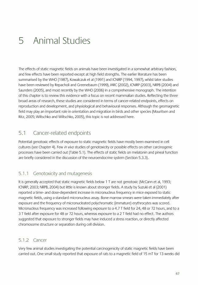
67
5 Animal Studies
The effects of static magnetic fields on animals have been investigated in a somewhat arbitrary fashion, and few effects have been reported except at high field strengths. The earlier literature has been summarised by the WHO (1987), Kowalczuk et al (1991) and ICNIRP (1994, 1997), whilst later studies have been reviewed by Repacholi and Greenebaum (1999), IARC (2002), ICNIRP (2003), NRPB (2004) and Saunders (2005), and most recently by the WHO (2006) in a comprehensive monograph. The intention of this chapter is to review this evidence with a focus on recent mammalian studies. Reflecting the three broad areas of research, these studies are considered in terms of cancer-related endpoints, effects on reproduction and development, and physiological and behavioural responses. Although the geomagnetic field may play an important role in orientation and migration in birds and other species (Mouritsen and Ritz, 2005; Wiltschko and Wiltschko, 2005), this topic is not addressed here.
5.1 Cancer-related endpoints
Potential genotoxic effects of exposure to static magnetic fields have mostly been examined in cell cultures (see Chapter 4). Few in vivo studies of genotoxicity or possible effects on other carcinogenic processes have been carried out (Table 5.1). The effects of static fields on melatonin and pineal function are briefly considered in the discussion of the neuroendocrine system (Section 5.3.3).
5.1.1 Genotoxicity and mutagenesis
It is generally accepted that static magnetic fields below 1 T are not genotoxic (McCann et al, 1993; ICNIRP, 2003; NRPB, 2004) but little is known about stronger fields. A study by Suzuki et al (2001) reported a time- and dose-dependent increase in micronucleus frequency in mice exposed to static magnetic fields, using a standard micronucleus assay. Bone marrow smears were taken immediately after exposure and the frequency of micronucleated polychromatic (immature) erythrocytes was scored. Micronucleus frequency was increased following exposure to a 4.7 T field for 24, 48 or 72 hours, and to a 3 T field after exposure for 48 or 72 hours, whereas exposure to a 2 T field had no effect. The authors suggested that exposure to stronger fields may have induced a stress reaction, or directly affected chromosome structure or separation during cell division.
5.1.2 Cancer
Very few animal studies investigating the potential carcinogenicity of static magnetic fields have been carried out. One small study reported that exposure of rats to a magnetic field of 15 mT for 13 weeks did
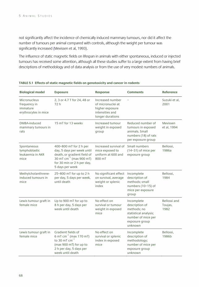
5 A N I M A L S T U D I E S
68
not significantly affect the incidence of chemically induced mammary tumours, nor did it affect the number of tumours per animal compared with controls, although the weight per tumour was significantly increased (Mevissen et al, 1993).
The influence of static magnetic fields on lifespan in animals with either spontaneous, induced or injected tumours has received some attention, although all these studies suffer to a large extent from having brief descriptions of methodology and of data analysis or from the use of very modest numbers of animals.
TABLE 5.1 Effects of static magnetic fields on genotoxicity and cancer in rodents
Biological model Exposure Response Comments Reference
Micronucleus frequency in immature erythrocytes in mice
2, 3 or 4.7 T for 24, 48 or 72 h
Increased number of micronuclei at higher exposure intensities and longer durations
– Suzuki et al, 2001
DMBA-induced mammary tumours in rats
15 mT for 13 weeks Increased tumour weight in exposed group
Reduced number of tumours in exposed animals. Small numbers (18) of rats per exposure group
Mevissen et al, 1994
Spontaneous lymphoblastic leukaemia in AKR mice
400–800 mT for 2 h per day, 5 days per week until death, or gradient field of 30 mT cm–1 (max 900 mT) for 30 min or 2 h per day, 5 days per week
Increased survival of mice exposed to uniform at 600 and 800 mT
Small numbers (14–31) of mice per exposure group
Bellossi, 1986a
Methylcholanthrene-induced tumours in mice
25–800 mT for up to 2 h per day, 5 days per week, until death
No significant effect on survival, average weight or splenic index
Incomplete description of methods; small numbers (10–15) of mice per exposure group
Bellossi, 1984
Lewis tumour graft in female mice
Up to 900 mT for up to 8 h per day, 5 days per week until death
No effect on survival or tumour weight in exposed mice
Incomplete description of methods; no statistical analysis; number of mice per exposure group unknown
Bellossi and Toujas, 1982
Lewis tumour graft in female mice
Gradient fields of 6 mT cm–1 (max 170 mT) to 30 mT cm–1 (max 900 mT) for up to 2 h per day, 5 days per week until death
No effect on survival or splenic index in exposed mice
Incomplete description of methodology; number of mice per exposure group unknown
Bellossi, 1986b
R E P R O D U C T I O N A N D D E V E L O P M E N T
69
Bellossi (1986a) investigated the effect of exposure to uniform and gradient static magnetic fields using AKR mice which develop spontaneous viral lymphoblastic leukaemia. Exposures at 600 and 800 mT (but not 400 mT) were reported to increase survival, but the numbers of animals used in these groups were very small. Bellossi (1984) reported that exposure at up to 800 mT did not affect the survival time of mice with chemically induced tumours.
Bellossi and Toujas (1982) reported that daily, long-term exposure to uniform magnetic fields of up to around 1 T had no effect on the survival of mice injected with Lewis lung tumour cells. It was suggested that exposure increased the growth rate of the tumours, but this was not quantified. Using the same model, Bellossi (1986b) found survival was not affected by exposure to non-uniform fields with gradients of up to 3 T m−1.
5.2 Reproduction and development
Only a few studies have examined the effect of static magnetic fields on fertility; most have investigated possible effects on the developing embryo and fetus (teratogenic effects).
5.2.1 Fertility
The available evidence concerning the effects of static magnetic fields on fertility is limited, although it does not suggest that exposure is capable of causing any consistent deleterious effect (Table 5.2). Withers et al (1985) detected no effect on spermatogenesis after the exposure of mice at 0.3 T for 66 hours. However, Narra et al (1996) reported slight and variable changes in spermatogenesis and embryogenesis in mice exposed at 1.5 T for 30 minutes. Tablado et al (1996, 1998) reported that maturation of sperm movement in adult mice was largely unaffected by either single, short-term exposure or continuous, long-term exposure at 0.7 T. No effects on sperm motility, maturation and production were reported after exposing adult mice to up to 0.7 T for a maximum of 35 days (Tablado et al, 1996). Later, using the same experimental set up, increased levels of sperm head abnormalities (lack of a ‘hook’) were observed in exposed adult mice (Tablado et al, 1998).
5.2.2 Growth and development
Several studies have explored the possible teratogenic effects of exposure to static magnetic fields (Table 5.3). An early study by Sikov et al (1979) found no effect of exposure to a uniform static field of 1 T or to a field gradient of 2.5 T m–1 with a maximum flux density of 1 T, on the prenatal and postnatal development of mice. Exposure took place over the whole of gestation, or before implantation, during organogenesis or during fetal development. Animals used for prenatal evaluation were killed on day 18 of gestation and evaluated for external and internal malformations and for skeletal defects. Postnatal development was assessed from the appearance of various developmental landmarks and simple behavioural reflexes. There were no differences between the exposed and sham-exposed groups in the number of pregnancies, which was low (down to 14% in one sham-exposed group) and variable in both
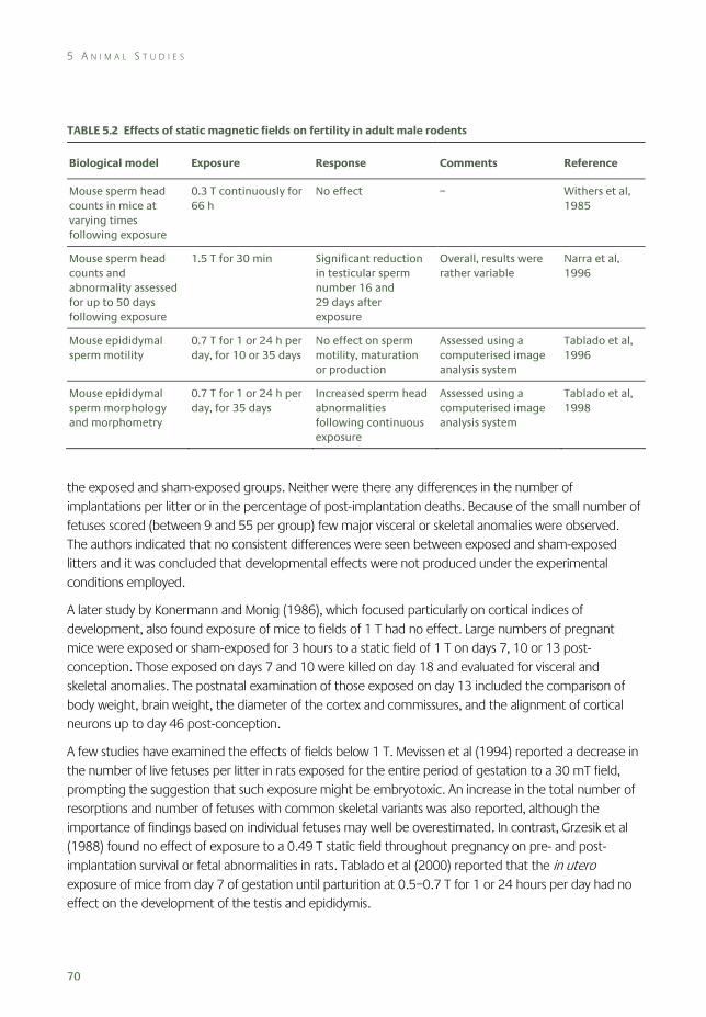
5 A N I M A L S T U D I E S
70
TABLE 5.2 Effects of static magnetic fields on fertility in adult male rodents
Biological model Exposure Response Comments Reference
Mouse sperm head counts in mice at varying times following exposure
0.3 T continuously for 66 h
No effect – Withers et al, 1985
Mouse sperm head counts and abnormality assessed for up to 50 days following exposure
1.5 T for 30 min Significant reduction in testicular sperm number 16 and 29 days after exposure
Overall, results were rather variable
Narra et al, 1996
Mouse epididymal sperm motility
0.7 T for 1 or 24 h per day, for 10 or 35 days
No effect on sperm motility, maturation or production
Assessed using a computerised image analysis system
Tablado et al, 1996
Mouse epididymal sperm morphology and morphometry
0.7 T for 1 or 24 h per day, for 35 days
Increased sperm head abnormalities following continuous exposure
Assessed using a computerised image analysis system
Tablado et al, 1998
the exposed and sham-exposed groups. Neither were there any differences in the number of implantations per litter or in the percentage of post-implantation deaths. Because of the small number of fetuses scored (between 9 and 55 per group) few major visceral or skeletal anomalies were observed. The authors indicated that no consistent differences were seen between exposed and sham-exposed litters and it was concluded that developmental effects were not produced under the experimental conditions employed.
A later study by Konermann and Monig (1986), which focused particularly on cortical indices of development, also found exposure of mice to fields of 1 T had no effect. Large numbers of pregnant mice were exposed or sham-exposed for 3 hours to a static field of 1 T on days 7, 10 or 13 post-conception. Those exposed on days 7 and 10 were killed on day 18 and evaluated for visceral and skeletal anomalies. The postnatal examination of those exposed on day 13 included the comparison of body weight, brain weight, the diameter of the cortex and commissures, and the alignment of cortical neurons up to day 46 post-conception.
A few studies have examined the effects of fields below 1 T. Mevissen et al (1994) reported a decrease in the number of live fetuses per litter in rats exposed for the entire period of gestation to a 30 mT field, prompting the suggestion that such exposure might be embryotoxic. An increase in the total number of resorptions and number of fetuses with common skeletal variants was also reported, although the importance of findings based on individual fetuses may well be overestimated. In contrast, Grzesik et al (1988) found no effect of exposure to a 0.49 T static field throughout pregnancy on pre- and post-implantation survival or fetal abnormalities in rats. Tablado et al (2000) reported that the in utero exposure of mice from day 7 of gestation until parturition at 0.5–0.7 T for 1 or 24 hours per day had no effect on the development of the testis and epididymis.
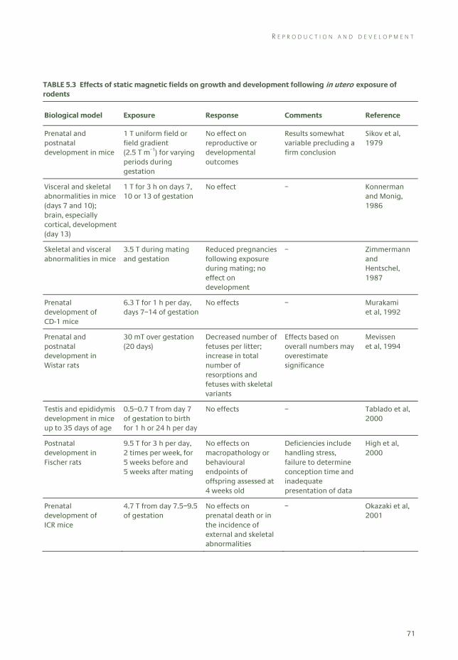
R E P R O D U C T I O N A N D D E V E L O P M E N T
71
TABLE 5.3 Effects of static magnetic fields on growth and development following in utero exposure of rodents
Biological model Exposure Response Comments Reference
Prenatal and postnatal development in mice
1 T uniform field or field gradient (2.5 T m–1) for varying periods during gestation
No effect on reproductive or developmental outcomes
Results somewhat variable precluding a firm conclusion
Sikov et al, 1979
Visceral and skeletal abnormalities in mice (days 7 and 10); brain, especially cortical, development (day 13)
1 T for 3 h on days 7, 10 or 13 of gestation
No effect – Konnerman and Monig, 1986
Skeletal and visceral abnormalities in mice
3.5 T during mating and gestation
Reduced pregnancies following exposure during mating; no effect on development
– Zimmermann and Hentschel, 1987
Prenatal development of CD-1 mice
6.3 T for 1 h per day, days 7–14 of gestation
No effects – Murakami et al, 1992
Prenatal and postnatal development in Wistar rats
30 mT over gestation (20 days)
Decreased number of fetuses per litter; increase in total number of resorptions and fetuses with skeletal variants
Effects based on overall numbers may overestimate significance
Mevissen et al, 1994
Testis and epididymis development in mice up to 35 days of age
0.5–0.7 T from day 7 of gestation to birth for 1 h or 24 h per day
No effects – Tablado et al, 2000
Postnatal development in Fischer rats
9.5 T for 3 h per day, 2 times per week, for 5 weeks before and 5 weeks after mating
No effects on macropathology or behavioural endpoints of offspring assessed at 4 weeks old
Deficiencies include handling stress, failure to determine conception time and inadequate presentation of data
High et al, 2000
Prenatal development of ICR mice
4.7 T from day 7.5–9.5 of gestation
No effects on prenatal death or in the incidence of external and skeletal abnormalities
– Okazaki et al, 2001
5 A N I M A L S T U D I E S
72
The few studies that have investigated the effects of exposure of mice to static fields above 1 T have reported no consistent field-dependent effects. Zimmermann and Hentschel (1987) exposed mice throughout gestation to a field of 3.5 T and found no effects on embryonic and fetal development, including a lack of visceral and skeletal anomalies. However, exposure during mating resulted in a reduced pregnancy outcome. Murakamui et al (1992) exposed mice to a field of 6.3 T for one hour per day over the major period of organogenesis, and examined the fetuses at the end of gestation. No significant differences were seen between exposed and control groups regarding litter size, fetal weight, intrauterine mortality or external and skeletal abnormalities. Okazaki et al (2001) exposed pregnant mice to a 4.7 T field for two days during the middle of gestation and examined the fetuses at birth. There were no significant differences in the incidence of prenatal death or in the incidence of external and skeletal abnormalities. However, exposure promoted endochondral ossification of chondrocytes taken from the sternum of fetal mice.
The effects of exposure to very strong fields have as yet only received scant attention. As part of a larger study investigating the effects of static fields on haematology, biochemistry and behaviour in adult animals, High et al (2000) exposed young adult rats to a field of 9.4 T for three hours, twice a week for five weeks. The animals were anaesthetised during exposures to render them immobile. Exposures then ceased for two weeks, during which time animals were allowed to mate over a seven-day period. Animals were then exposed to the field again using the same schedule for a further five weeks. Since it is not clear that the actual day of mating was controlled or even recorded, the offspring could have been of differing gestational ages during exposure: it was only reported that exposure in utero took place during the embryonic and fetal stages. The offspring were assessed when four weeks old and no field-dependent effects were seen; however, no data were given describing the behavioural and neurophysiological evaluations, nor was any evidence presented regarding the incidence of gross abnormalities and macropathological findings. Thus the results of this study are uninterpretable.
5.3 Physiological and behavioural responses
The physiological responses to static magnetic field exposure can be grouped into four main themes: effects on the cardiovascular system, the nervous system, the neuroendocrine system, and on behavioural responses.
5.3.1 Cardiovascular effects
Electric potentials (flow potentials), generated across a blood vessel by the flow of blood in a static magnetic field, have been recorded by several groups of investigators in a number of animal species exposed to magnetic fields greater than about 100 mT. More widespread effects on cardiovascular function, particularly arterial blood pressure and peripheral blood flow, have also been extensively investigated, mostly using anaesthetised animals.
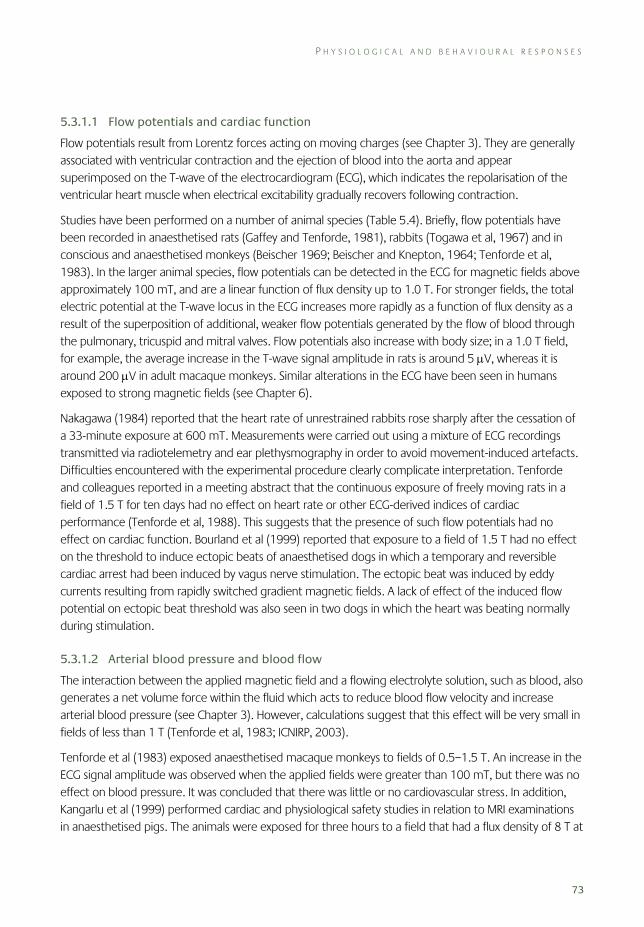
P H Y S I O L O G I C A L A N D B E H A V I O U R A L R E S P O N S E S
73
5.3.1.1 Flow potentials and cardiac function
Flow potentials result from Lorentz forces acting on moving charges (see Chapter 3). They are generally associated with ventricular contraction and the ejection of blood into the aorta and appear superimposed on the T-wave of the electrocardiogram (ECG), which indicates the repolarisation of the ventricular heart muscle when electrical excitability gradually recovers following contraction.
Studies have been performed on a number of animal species (Table 5.4). Briefly, flow potentials have been recorded in anaesthetised rats (Gaffey and Tenforde, 1981), rabbits (Togawa et al, 1967) and in conscious and anaesthetised monkeys (Beischer 1969; Beischer and Knepton, 1964; Tenforde et al, 1983). In the larger animal species, flow potentials can be detected in the ECG for magnetic fields above approximately 100 mT, and are a linear function of flux density up to 1.0 T. For stronger fields, the total electric potential at the T-wave locus in the ECG increases more rapidly as a function of flux density as a result of the superposition of additional, weaker flow potentials generated by the flow of blood through the pulmonary, tricuspid and mitral valves. Flow potentials also increase with body size; in a 1.0 T field, for example, the average increase in the T-wave signal amplitude in rats is around 5 μV, whereas it is around 200 μV in adult macaque monkeys. Similar alterations in the ECG have been seen in humans exposed to strong magnetic fields (see Chapter 6).
Nakagawa (1984) reported that the heart rate of unrestrained rabbits rose sharply after the cessation of a 33-minute exposure at 600 mT. Measurements were carried out using a mixture of ECG recordings transmitted via radiotelemetry and ear plethysmography in order to avoid movement-induced artefacts. Difficulties encountered with the experimental procedure clearly complicate interpretation. Tenforde and colleagues reported in a meeting abstract that the continuous exposure of freely moving rats in a field of 1.5 T for ten days had no effect on heart rate or other ECG-derived indices of cardiac performance (Tenforde et al, 1988). This suggests that the presence of such flow potentials had no effect on cardiac function. Bourland et al (1999) reported that exposure to a field of 1.5 T had no effect on the threshold to induce ectopic beats of anaesthetised dogs in which a temporary and reversible cardiac arrest had been induced by vagus nerve stimulation. The ectopic beat was induced by eddy currents resulting from rapidly switched gradient magnetic fields. A lack of effect of the induced flow potential on ectopic beat threshold was also seen in two dogs in which the heart was beating normally during stimulation.
5.3.1.2 Arterial blood pressure and blood flow
The interaction between the applied magnetic field and a flowing electrolyte solution, such as blood, also generates a net volume force within the fluid which acts to reduce blood flow velocity and increase arterial blood pressure (see Chapter 3). However, calculations suggest that this effect will be very small in fields of less than 1 T (Tenforde et al, 1983; ICNIRP, 2003).
Tenforde et al (1983) exposed anaesthetised macaque monkeys to fields of 0.5–1.5 T. An increase in the ECG signal amplitude was observed when the applied fields were greater than 100 mT, but there was no effect on blood pressure. It was concluded that there was little or no cardiovascular stress. In addition, Kangarlu et al (1999) performed cardiac and physiological safety studies in relation to MRI examinations in anaesthetised pigs. The animals were exposed for three hours to a field that had a flux density of 8 T at
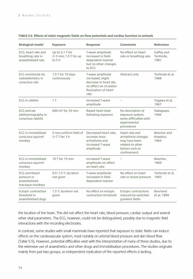
5 A N I M A L S T U D I E S
74
TABLE 5.4 Effects of static magnetic fields on flow potentials and cardiac function in animals
Biological model Exposure Response Comments Reference
ECG, heart rate and breathing rate in anaesthetised rats
Up to 2.1 T for 2–3 min; 1.5 T for up to 5 h
T-wave amplitude increased in field- dependent manner but no other changes to ECG
No effect on heart rate or breathing rate
Gaffey and Tenforde, 1981
ECG monitored via radiotelemetry in conscious rats
1.5 T for 10 days continuously
T-wave amplitude increased; slight decrease in heart ate, no effect on circadian fluctuation of heart rate
Abstract only Tenforde et al, 1988
ECG in rabbits 1 T Increased T-wave amplitude
– Togawa et al, 1967
ECG and ear plethysmography in conscious rabbits
600 mT for 33 min Raised heart beat following exposure
No description of exposure system; some difficulties with experimental procedures
Nakagawa, 1984
ECG in immobilised conscious squirrel monkey
A non-uniform field of 2–7 T for 3 h
Decreased heart rate, increase sinus arrhythmia and increased T-wave amplitude
Heart rate and arrhythmia changes may have been related to other factors such as confinement.
Beischer and Knepton, 1964
ECG in immobilised conscious squirrel monkey
10 T for 15 min Increased T-wave amplitude; no effect on heart rate
– Beischer, 1969
ECG and blood pressure in anaesthetised macaque monkeys
0.5–1.5 T; duration not given
T-wave amplitude increased in field- dependent manner
No effect on heart rate or blood pressure
Tenforde et al, 1983
Ectopic contraction threshold in anaesthetised dogs
1.5 T; duration not given
No effect on ectopic contraction threshold
Ectopic contractions induced by switched gradient fields
Bourland et al, 1999
the location of the heart. This did not affect the heart rate, blood pressure, cardiac output and several other vital parameters. The ECG, however, could not be distinguished, possibly due to magnetic field interactions with the recording electrodes.
In contrast, some studies with small mammals have reported that exposure to static fields can induce effects on the cardiovascular system, most notably on arterial blood pressure and skin blood flow (Table 5.5). However, potential difficulties exist with the interpretation of many of these studies, due to the extensive use of anaesthetics and other drugs and immobilisation procedures. The studies originate mainly from just two groups, so independent replication of the reported effects is lacking.
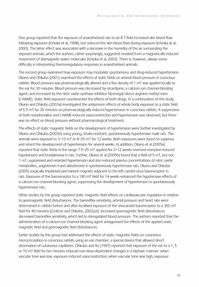
P H Y S I O L O G I C A L A N D B E H A V I O U R A L R E S P O N S E S
75
One group reported that the exposure of anaesthetised rats to an 8 T field increased skin blood flow following exposure (Ichioka et al, 1998), but reduced the skin blood flow during exposure (Ichioka at al, 2000). The latter effect was associated with a decrease in the humidity of the air surrounding the exposed animals, which the authors, rather surprisingly, suggested resulted from a magnetically induced movement of diamagnetic water molecules (Ichioka et al, 2003). There is, however, always some difficulty in interpreting thermoregulatory responses in anaesthetised animals.
The second group examined how exposure may modulate spontaneous and drug-induced hypertension. Okano and Ohkubo (2001) examined the effects of static fields on arterial blood pressure in conscious rabbits. Blood pressure was pharmacologically altered and a flux density of 1 mT was applied locally to the ear for 30 minutes. Blood pressure was decreased by nicardipine, a calcium ion channel-blocking agent, and increased by the nitric oxide synthase inhibitor N(omega)-nitro-L-arginine methyl ester (L-NAME). Static field exposure counteracted the effects of both drugs. In a continuation of this study, Okano and Ohkubo (2003a) investigated the antipressor effects of whole body exposure to a static field of 5.5 mT for 30 minutes on pharmacologically induced hypertension in conscious rabbits. A suppression of both noradrenaline and L-NAME-induced vasoconstriction and hypertension was observed, but there was no effect on blood pressure without pharmacological treatment.
The effects of static magnetic fields on the development of hypertension were further investigated by Okano and Ohkubo (2003b) using young, stroke-resistant, spontaneously hypertensive male rats. The animals were exposed to 3–10 mT or 8–25 mT for 12 weeks. Both exposures were found to suppress and retard the development of hypertension for several weeks. In addition, Okano et al (2005a) reported that static fields in the range 7.5–25 mT applied for 2–12 weeks reversed reserpine-induced hypotension and bradykinesia in rats. Further, Okano et al (2005b) found that a field of 5 mT, but not 1 mT, suppressed and retarded hypertension and also reduced plasma concentrations of nitric oxide metabolites, angiotensin II and aldosterone in spontaneously hypertensive rats. Okano and Ohkubo (2005) surgically implanted permanent magnets adjacent to the left carotid sinus baroreceptor in rats. Exposure of the baroreceptor to a 180 mT field for 14 weeks enhanced the hypotensive effects of a calcium ion channel-blocking agent, suppressing the development of hypertension in spontaneously hypertensive rats.
Other studies by this group reported static magnetic field effects on cardiovascular regulation in relation to geomagnetic field disturbances. The baroreflex sensitivity, arterial pressure and heart rate were determined in rabbits before and after localised exposure of the sinocarotid baroreceptor to a 350 mT field for 40 minutes (Gmitrov and Ohkubo, 2002a,b). Increased geomagnetic field disturbances decreased baroreflex sensitivity, which led to deregulated blood pressure. The authors reported that the administration of a calcium ion channel-blocking agent antagonised the effects of the applied static magnetic field and geomagnetic field disturbances.
Earlier studies by this group had addressed the effects of static magnetic fields on cutaneous microcirculation in conscious rabbits using an ear chamber, a special device that allowed direct observation of cutaneous capillaries. Ohkubo and Xu (1997) reported that exposure of the ear to a 1, 5 or 10 mT field for ten minutes induced non-dose-dependent changes in a biphasic manner: when vascular tone was low, exposure induced vasoconstriction; when vascular tone was high, exposure
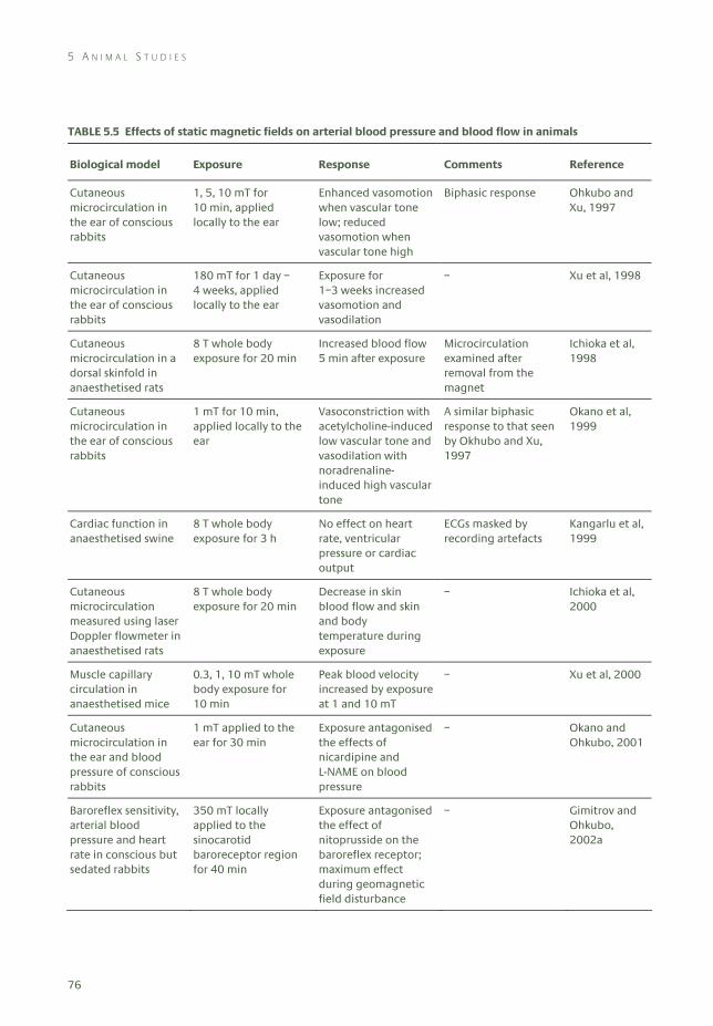
5 A N I M A L S T U D I E S
76
TABLE 5.5 Effects of static magnetic fields on arterial blood pressure and blood flow in animals
Biological model Exposure Response Comments Reference
Cutaneous microcirculation in the ear of conscious rabbits
1, 5, 10 mT for 10 min, applied locally to the ear
Enhanced vasomotion when vascular tone low; reduced vasomotion when vascular tone high
Biphasic response Ohkubo and Xu, 1997
Cutaneous microcirculation in the ear of conscious rabbits
180 mT for 1 day – 4 weeks, applied locally to the ear
Exposure for 1–3 weeks increased vasomotion and vasodilation
– Xu et al, 1998
Cutaneous microcirculation in a dorsal skinfold in anaesthetised rats
8 T whole body exposure for 20 min
Increased blood flow 5 min after exposure
Microcirculation examined after removal from the magnet
Ichioka et al, 1998
Cutaneous microcirculation in the ear of conscious rabbits
1 mT for 10 min, applied locally to the ear
Vasoconstriction with acetylcholine-induced low vascular tone and vasodilation with noradrenaline-induced high vascular tone
A similar biphasic response to that seen by Okhubo and Xu, 1997
Okano et al, 1999
Cardiac function in anaesthetised swine
8 T whole body exposure for 3 h
No effect on heart rate, ventricular pressure or cardiac output
ECGs masked by recording artefacts
Kangarlu et al, 1999
Cutaneous microcirculation measured using laser Doppler flowmeter in anaesthetised rats
8 T whole body exposure for 20 min
Decrease in skin blood flow and skin and body temperature during exposure
– Ichioka et al, 2000
Muscle capillary circulation in anaesthetised mice
0.3, 1, 10 mT whole body exposure for 10 min
Peak blood velocity increased by exposure at 1 and 10 mT
– Xu et al, 2000
Cutaneous microcirculation in the ear and blood pressure of conscious rabbits
1 mT applied to the ear for 30 min
Exposure antagonised the effects of nicardipine and L-NAME on blood pressure
– Okano and Ohkubo, 2001
Baroreflex sensitivity, arterial blood pressure and heart rate in conscious but sedated rabbits
350 mT locally applied to the sinocarotid baroreceptor region for 40 min
Exposure antagonised the effect of nitoprusside on the baroreflex receptor; maximum effect during geomagnetic field disturbance
– Gimitrov and Ohkubo, 2002a
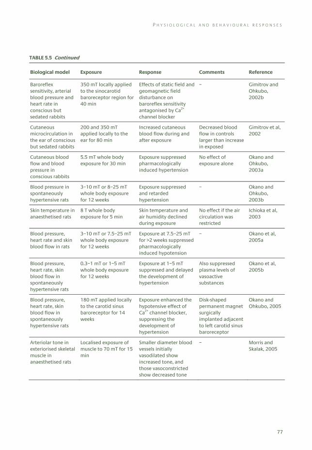
P H Y S I O L O G I C A L A N D B E H A V I O U R A L R E S P O N S E S
77
TABLE 5.5 Continued
Biological model Exposure Response Comments Reference
Baroreflex sensitivity, arterial blood pressure and heart rate in conscious but sedated rabbits
350 mT locally applied to the sinocarotid baroreceptor region for 40 min
Effects of static field and geomagnetic field disturbance on baroreflex sensitivity antagonised by Ca2+ channel blocker
– Gimitrov and Ohkubo, 2002b
Cutaneous microcirculation in the ear of conscious but sedated rabbits
200 and 350 mT applied locally to the ear for 80 min
Increased cutaneous blood flow during and after exposure
Decreased blood flow in controls larger than increase in exposed
Gimitrov et al, 2002
Cutaneous blood flow and blood pressure in conscious rabbits
5.5 mT whole body exposure for 30 min
Exposure suppressed pharmacologically induced hypertension
No effect of exposure alone
Okano and Ohkubo, 2003a
Blood pressure in spontaneously hypertensive rats
3–10 mT or 8–25 mT whole body exposure for 12 weeks
Exposure suppressed and retarded hypertension
– Okano and Ohkubo, 2003b
Skin temperature in anaesthetised rats
8 T whole body exposure for 5 min
Skin temperature and air humidity declined during exposure
No effect if the air circulation was restricted
Ichioka et al, 2003
Blood pressure, heart rate and skin blood flow in rats
3–10 mT or 7.5–25 mT whole body exposure for 12 weeks
Exposure at 7.5–25 mT for >2 weeks suppressed pharmacologically induced hypotension
– Okano et al, 2005a
Blood pressure, heart rate, skin blood flow in spontaneously hypertensive rats
0.3–1 mT or 1–5 mT whole body exposure for 12 weeks
Exposure at 1–5 mT suppressed and delayed the development of hypertension
Also suppressed plasma levels of vasoactive substances
Okano et al, 2005b
Blood pressure, heart rate, skin blood flow in spontaneously hypertensive rats
180 mT applied locally to the carotid sinus baroreceptor for 14 weeks
Exposure enhanced the hypotensive effect of Ca2+ channel blocker, suppressing the development of hypertension
Disk-shaped permanent magnet surgically implanted adjacent to left carotid sinus baroreceptor
Okano and Ohkubo, 2005
Arteriolar tone in exteriorised skeletal muscle in anaesthetised rats
Localised exposure of muscle to 70 mT for 15 min
Smaller diameter blood vessels initially vasodilated show increased tone, and those vasoconstricted show decreased tone
– Morris and Skalak, 2005
5 A N I M A L S T U D I E S
78
induced vasodilatation. Okano et al (1999) performed a more extensive investigation of this effect. They exposed the ears of conscious rabbits to a 1 mT field for ten minutes while either increasing the vascular tone by noradrenaline administration, or decreasing it using acetylcholine. Static magnetic fields resulted in vasodilatation and increased vasomotion under high vascular tone, and in vasoconstriction and decreased vasomotion under low vascular tone. Thus, static magnetic fields appeared to counteract the effects of the applied drugs. The long-term effects of a locally applied static magnetic field on cutaneous microcirculation in rabbits were investigated by Xu et al (1998). Exposure of the ear to a 180 mT field for one to three weeks significantly increased the amplitude of long-lasting vasodilatation and enhanced the vasomotion. The changes in vasomotion returned to their initial values after exposure ceased.
Other studies have examined muscle and cutaneous blood flow in anaesthetised animals. Xu et al (2000) studied acute microhaemodynamic effects of whole body exposure to fields of 0.3, 1 and 10 mT for ten minutes in anaesthetised mice. An increased peak blood velocity in muscle tissue was observed for fields of 1 mT or higher. The effect persisted for up to 35 hours after exposure. In addition, Gmitrov et al (2002) reported that exposure of the ear of anaesthetised rabbits to 200 and 350 mT fields increased cutaneous blood flow in the ear during and after exposure.
More recently, a study by Morris and Skalak (2005) reported that localised exposure to a static field of 70 mT for 15 minutes of the exteriorised skeletal muscle of an anaesthetised rat altered vascular tone as assessed by measurement of vessel diameter. Arteriolar vessels with an initial tone of less than 15% showed a rapid increase in tone, and those with an initial tone greater than 15% showed a rapid decrease in tone.
5.3.2 Nervous system responses
Several studies have investigated the electrophysiological responses of nervous tissues to static magnetic fields (Table 5.6). Schwartz (1978, 1979) found no effect of a 1.2 T field on action potential conduction velocity and ion channel currents in isolated lobster giant axon preparations. Similarly, Gaffey and Tenforde (1983) found no effect of exposure to a 2 T field for 4 or 17 hours on conduction velocity and refractory period in excised frog sciatic nerve preparation. It was also reported that exposure to a 1 T field had no effect on nerve excitation threshold. Using the same preparation, Osuga and Tatsuoka (1999) reported a lack of effect of a 1.5 T field on action potential conduction velocity. However, in this study, exposure was carried out two hours after nerve extraction, so the possibility exists that the electrical properties of the nerve may have partially decayed.
Ye et al (2004) reported that exposure of the giant axons of crayfish to a static field in the range 8–43 mT slightly increased the amplitude of induced action potentials (around 6%) and the resulting excitatory post-synaptic potentials (around 20%) in a manner that depended on the amplitude and duration of exposure: the action potential amplitude increased by exposure at 8 mT for three hours, but not at 17 or 43 mT, and that exposure for five minutes at any of these three flux densities resulted in an increased amplitude three hours later. The authors speculated that the static field had sensitised the animal’s escape reflex to external stimuli.
P H Y S I O L O G I C A L A N D B E H A V I O U R A L R E S P O N S E S
79
In contrast, McLean and colleagues found that a static field of 11 mT blocked the electrical induction of action potentials in 66% of cultured mouse primary dorsal root ganglion neurons, compared with a background failure rate of less than 5% (McLean et al, 1991, 1995; Cavopol et al, 1995). The number of failures was maximal after 200–250 seconds in the field and afterwards gradually returned to control values over 200–600 seconds. Different combinations of small permanent magnets had different effects; the authors concluded that both the amplitude and gradient of the magnetic field affected the experimental outcome.
Hong et al (1986) found exposure to fields of up to 1.2 T had no effect on motor nerve conduction velocity in the tails of anaesthetised rats, but reported a significant increase in the amplitude of the resulting compound action potentials recorded in the muscle fibres of the tail following sub-maximal nerve stimulation and exposure to fields of more than 0.5 T for longer than 30 seconds. Contradictory results were described by Itegin et al (1995), who reported that the chronic exposure of rats to a field of only 0.2 mT resulted in a decreased resting membrane potential, action potential amplitude and contraction force recorded from muscle fibres in isolated phrenic nerve-diaphragm muscle preparations. These effects were attributed to an observed increase in Ca2+-ATPase activity.
Rosen and colleagues have carried out a number of electrophysiological studies over the past 10–20 years, including in vitro as well as in vivo studies (see Rosen, 2003a, for review). For example, Rosen (1992, 1993, 1994) reported that exposure to a 120 mT magnetic field resulted in a decrease in the frequency of miniature endplate potentials recorded from a mouse phrenic nerve-diaphragm muscle preparation at temperatures above 35°C. This was not seen when using a calcium-ion-free perfusate, suggesting that neurotransmitter release was affected. The author speculated that this resulted from the slow re-orientation of aligned groups of diamagnetic phospholipid molecules within the cell membrane distorting and thereby affecting ion channel function.
A later series of studies using whole-cell patch clamp techniques to record from cultured GH3 pituitary cells investigated the effects of exposure to a 120 mT static magnetic field on voltage-gated calcium and sodium ion channel kinetics. Rosen (1996), for example, reported a slowing of the activation rate (an increase in the activation time constant) of voltage-activated calcium ion channels at negative membrane potentials during and after exposure to a 120 mT static magnetic field. This increase lasted during and at least 100 seconds after exposure, but there was no change in the inactivation time constant. Rosen (2003b) found that exposure also resulted in a slow but pronounced (up to 200%) increase in the activation time constant of the voltage-gated sodium ion channels. In principle, changes in ion channel kinetics should be reflected in changes in excitation, conduction and recovery, in apparent contrast to the lack of effect on action potential conduction velocity reported above. However, calculation by Hinch et al (2005), using the Hodgkin-Huxley equations, revealed that the effect of increasing the sodium ion channel activation time constant would have had only a very small effect on the action potential conduction velocity and refractory period.
In contrast to these results, Sonnier et al (2000, 2003) found no changes in the resting membrane potential or action potential in neuroblastoma cells following brief exposures to fields of up to 7.5 mT. These included measurements, also based on patch-clamp methods, of the activation and inactivation time constants of sodium ion channels and the inactivation rate of the potassium ion channel. It was also

5 A N I M A L S T U D I E S
80
TABLE 5.6 Effects of static magnetic fields on electrophysiological responses
Biological assay Exposure Response Comments Reference
Somatosensory evoked potentials in anaesthetised rats
50–400 mT for 10–20 min
Change in waveform and increase in amplitude of evoked potentials
[Cited by WHO, 2006] Klimovskaya and Smirnova, 1976
Lobster giant axon preparation nerve conduction velocity etc
1.2 T parallel or perpendicular to the axon
No effect on action potential conduction velocity, membrane resting potential or transmembrane currents
Preparation declined after 10–15 min
Schwartz, 1978, 1979
Somatosensory evoked potentials in anaesthetised rats
0.1–1.6 T for 15 or 30 min
Intensity-dependent changes in form and amplitude of evoked potentials in cortex and hippocampus
[Cited by WHO, 2006] Smirnova et al, 1982
Excised frog sciatic nerve conduction properties
2 T parallel or perpendicular to the nerve for 4 or 17 h
No effect on conduction velocity or absolute or relative refractory period
In a separate study, 1 T perpendicular to the nerve had no effect on excitation threshold
Gaffey and Tenforde, 1983
EEGs of conscious rabbits
0.6 T for 33 min No effect on latency or amplitude of evoked potentials
EEG recordings prone to movement artefacts
Nakagawa, 1984
Motor nerve conduction velocity in anaesthetised rat tail
0.3–1.2 T for 15, 30 or 60 s
No effect on nerve conduction velocity. Increased muscle action potential amplitude following sub-maximal nerve stimulation
No effect following maximal nerve stimulation
Hong et al, 1986
Visual evoked potentials in the striate cortex of decerebrate cat brain
80, 120 mT for 100 s Long-lasting decrease in evoked potential amplitude and variability at 120 mT
Variable results at 80 mT
Rosen and Lubowsky, 1987
Spontaneous activity in neurons in the lateral geniculate body of decerebrate cat brain
123 mT for 100 s Long-lasting decrease in the spontaneous activity of 45% of neurons
– Rosen and Lubowsky, 1990
Somatosensory evoked potentials in the EEG of anaesthetised cats
Up to 4.7 T for 10 min No effect on evoked potential amplitude
Variable EEG frequency and amplitude over the experimental period
Kloiber et al, 1990
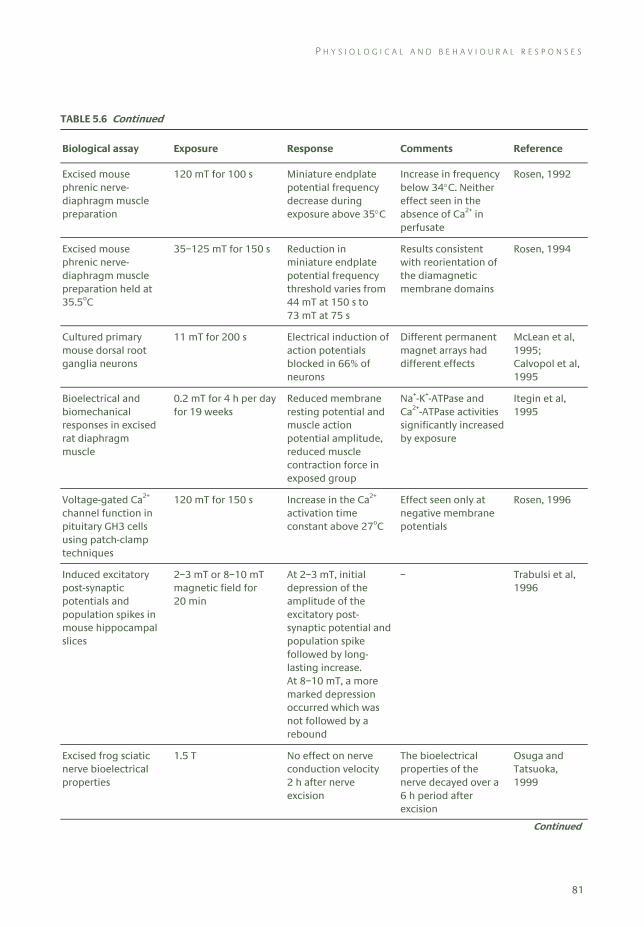
P H Y S I O L O G I C A L A N D B E H A V I O U R A L R E S P O N S E S
81
TABLE 5.6 Continued
Biological assay Exposure Response Comments Reference
Excised mouse phrenic nerve-diaphragm muscle preparation
120 mT for 100 s Miniature endplate potential frequency decrease during exposure above 35°C
Increase in frequency below 34°C. Neither effect seen in the absence of Ca2+ in perfusate
Rosen, 1992
Excised mouse phrenic nerve-diaphragm muscle preparation held at 35.5oC
35–125 mT for 150 s Reduction in miniature endplate potential frequency threshold varies from 44 mT at 150 s to 73 mT at 75 s
Results consistent with reorientation of the diamagnetic membrane domains
Rosen, 1994
Cultured primary mouse dorsal root ganglia neurons
11 mT for 200 s Electrical induction of action potentials blocked in 66% of neurons
Different permanent magnet arrays had different effects
McLean et al, 1995; Calvopol et al, 1995
Bioelectrical and biomechanical responses in excised rat diaphragm muscle
0.2 mT for 4 h per day for 19 weeks
Reduced membrane resting potential and muscle action potential amplitude, reduced muscle contraction force in exposed group
Na+-K+-ATPase and Ca2+-ATPase activities significantly increased by exposure
Itegin et al, 1995
Voltage-gated Ca2+ channel function in pituitary GH3 cells using patch-clamp techniques
120 mT for 150 s Increase in the Ca2+ activation time constant above 27oC
Effect seen only at negative membrane potentials
Rosen, 1996
Induced excitatory post-synaptic potentials and population spikes in mouse hippocampal slices
2–3 mT or 8–10 mT magnetic field for 20 min
At 2–3 mT, initial depression of the amplitude of the excitatory post-synaptic potential and population spike followed by long-lasting increase. At 8–10 mT, a more marked depression occurred which was not followed by a rebound
– Trabulsi et al, 1996
Excised frog sciatic nerve bioelectrical properties
1.5 T No effect on nerve conduction velocity 2 h after nerve excision
The bioelectrical properties of the nerve decayed over a 6 h period after excision
Osuga and Tatsuoka, 1999
Continued
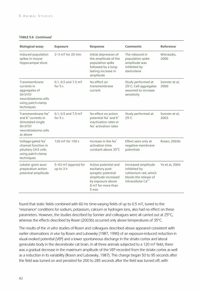
5 A N I M A L S T U D I E S
82
TABLE 5.6 Continued
Biological assay Exposure Response Comments Reference
Induced population spikes in mouse hippocampal slices
2–3 mT for 20 min Initial depression of the amplitude of the population spike followed by a long-lasting increase in amplitude
The rebound in population spike amplitude was inhibited by dantrolene
Wieraszko, 2000
Transmembrane currents in aggregates of SH-SY5Y neuroblastoma cells using patch-clamp techniques
0.1, 0.5 and 7.5 mT for 5 s
No effect on transmembrane current
Study performed at 25°C. Cell aggregates assumed to increase sensitivity
Sonnier et al, 2000
Transmembrane Na+ and K+ currents in stimulated single SH-SY5Y neuroblastoma cells as above
0.1, 0.5 and 7.5 mT for 5 s
No effect on action potential Na+ and K+ inactivation rates or Na+ activation rates
Study performed at 25°C
Sonnier et al, 2003
Voltage-gated Na+ channel function in pituitary GH3 cells using patch-clamp techniques
120 mT for 150 s Increase in the Na+ activation time constant above 35oC
Effect seen only at negative membrane potentials
Rosen, 2003b
Lobster giant axon preparation action potential amplitude
5–43 mT (approx) for up to 3 h
Action potential and excitatory post-synaptic potential amplitude increased by exposure above 8 mT for more than 5 min
Increased amplitude inhibited by ruthenium red, which blocks the release of intracellular Ca2+
Ye et al, 2004
found that static fields combined with 60 Hz time-varying fields of up to 0.5 mT, tuned to the ‘resonance’ conditions for sodium, potassium, calcium or hydrogen ions, also had no effect on these parameters. However, the studies described by Sonnier and colleagues were all carried out at 25°C, whereas the effects described by Rosen (2003b) occurred only above temperatures of 35°C.
The results of the in vitro studies of Rosen and colleagues described above appeared consistent with earlier observations in vivo by Rosen and Lubowsky (1987, 1990) of an exposure-induced reduction in visual evoked potential (VEP) and a lower spontaneous discharge in the striate cortex and lateral geniculate body in the decerebrate cat brain. In all three animals subjected to a 120 mT field, there was a gradual decrease in the maximum amplitude of the VEP recorded from the striate cortex as well as a reduction in its variability (Rosen and Lubowsky, 1987). This change began 50 to 95 seconds after the field was turned on and persisted for 200 to 285 seconds after the field was turned off, with
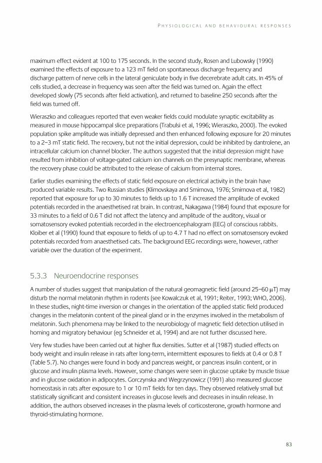
P H Y S I O L O G I C A L A N D B E H A V I O U R A L R E S P O N S E S
83
maximum effect evident at 100 to 175 seconds. In the second study, Rosen and Lubowsky (1990) examined the effects of exposure to a 123 mT field on spontaneous discharge frequency and discharge pattern of nerve cells in the lateral geniculate body in five decerebrate adult cats. In 45% of cells studied, a decrease in frequency was seen after the field was turned on. Again the effect developed slowly (75 seconds after field activation), and returned to baseline 250 seconds after the field was turned off.
Wieraszko and colleagues reported that even weaker fields could modulate synaptic excitability as measured in mouse hippocampal slice preparations (Trabulsi et al, 1996; Wieraszko, 2000). The evoked population spike amplitude was initially depressed and then enhanced following exposure for 20 minutes to a 2–3 mT static field. The recovery, but not the initial depression, could be inhibited by dantrolene, an intracellular calcium ion channel blocker. The authors suggested that the initial depression might have resulted from inhibition of voltage-gated calcium ion channels on the presynaptic membrane, whereas the recovery phase could be attributed to the release of calcium from internal stores.
Earlier studies examining the effects of static field exposure on electrical activity in the brain have produced variable results. Two Russian studies (Klimovskaya and Smirnova, 1976; Smirnova et al, 1982) reported that exposure for up to 30 minutes to fields up to 1.6 T increased the amplitude of evoked potentials recorded in the anaesthetised rat brain. In contrast, Nakagawa (1984) found that exposure for 33 minutes to a field of 0.6 T did not affect the latency and amplitude of the auditory, visual or somatosensory evoked potentials recorded in the electroencephalogram (EEG) of conscious rabbits. Kloiber et al (1990) found that exposure to fields of up to 4.7 T had no effect on somatosensory evoked potentials recorded from anaesthetised cats. The background EEG recordings were, however, rather variable over the duration of the experiment.
5.3.3 Neuroendocrine responses
A number of studies suggest that manipulation of the natural geomagnetic field (around 25–60 μT) may disturb the normal melatonin rhythm in rodents (see Kowalczuk et al, 1991; Reiter, 1993; WHO, 2006). In these studies, night-time inversion or changes in the orientation of the applied static field produced changes in the melatonin content of the pineal gland or in the enzymes involved in the metabolism of melatonin. Such phenomena may be linked to the neurobiology of magnetic field detection utilised in homing and migratory behaviour (eg Schneider et al, 1994) and are not further discussed here.
Very few studies have been carried out at higher flux densities. Sutter et al (1987) studied effects on body weight and insulin release in rats after long-term, intermittent exposures to fields at 0.4 or 0.8 T (Table 5.7). No changes were found in body and pancreas weight, or pancreas insulin content, or in glucose and insulin plasma levels. However, some changes were seen in glucose uptake by muscle tissue and in glucose oxidation in adipocytes. Gorczynska and Wegrzynowicz (1991) also measured glucose homeostasis in rats after exposure to 1 or 10 mT fields for ten days. They observed relatively small but statistically significant and consistent increases in glucose levels and decreases in insulin release. In addition, the authors observed increases in the plasma levels of corticosterone, growth hormone and thyroid-stimulating hormone.
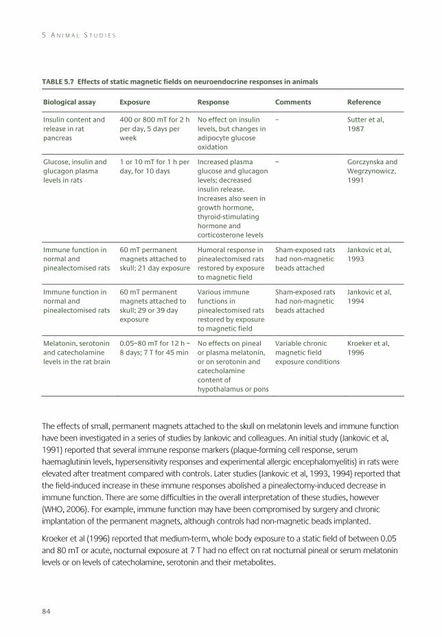
5 A N I M A L S T U D I E S
84
TABLE 5.7 Effects of static magnetic fields on neuroendocrine responses in animals
Biological assay Exposure Response Comments Reference
Insulin content and release in rat pancreas
400 or 800 mT for 2 h per day, 5 days per week
No effect on insulin levels, but changes in adipocyte glucose oxidation
– Sutter et al, 1987
Glucose, insulin and glucagon plasma levels in rats
1 or 10 mT for 1 h per day, for 10 days
Increased plasma glucose and glucagon levels; decreased insulin release. Increases also seen in growth hormone, thyroid-stimulating hormone and corticosterone levels
– Gorczynska and Wegrzynowicz, 1991
Immune function in normal and pinealectomised rats
60 mT permanent magnets attached to skull; 21 day exposure
Humoral response in pinealectomised rats restored by exposure to magnetic field
Sham-exposed rats had non-magnetic beads attached
Jankovic et al, 1993
Immune function in normal and pinealectomised rats
60 mT permanent magnets attached to skull; 29 or 39 day exposure
Various immune functions in pinealectomised rats restored by exposure to magnetic field
Sham-exposed rats had non-magnetic beads attached
Jankovic et al, 1994
Melatonin, serotonin and catecholamine levels in the rat brain
0.05–80 mT for 12 h – 8 days; 7 T for 45 min
No effects on pineal or plasma melatonin, or on serotonin and catecholamine content of hypothalamus or pons
Variable chronic magnetic field exposure conditions
Kroeker et al, 1996
The effects of small, permanent magnets attached to the skull on melatonin levels and immune function have been investigated in a series of studies by Jankovic and colleagues. An initial study (Jankovic et al, 1991) reported that several immune response markers (plaque-forming cell response, serum haemaglutinin levels, hypersensitivity responses and experimental allergic encephalomyelitis) in rats were elevated after treatment compared with controls. Later studies (Jankovic et al, 1993, 1994) reported that the field-induced increase in these immune responses abolished a pinealectomy-induced decrease in immune function. There are some difficulties in the overall interpretation of these studies, however (WHO, 2006). For example, immune function may have been compromised by surgery and chronic implantation of the permanent magnets, although controls had non-magnetic beads implanted.
Kroeker et al (1996) reported that medium-term, whole body exposure to a static field of between 0.05 and 80 mT or acute, nocturnal exposure at 7 T had no effect on rat nocturnal pineal or serum melatonin levels or on levels of catecholamine, serotonin and their metabolites.
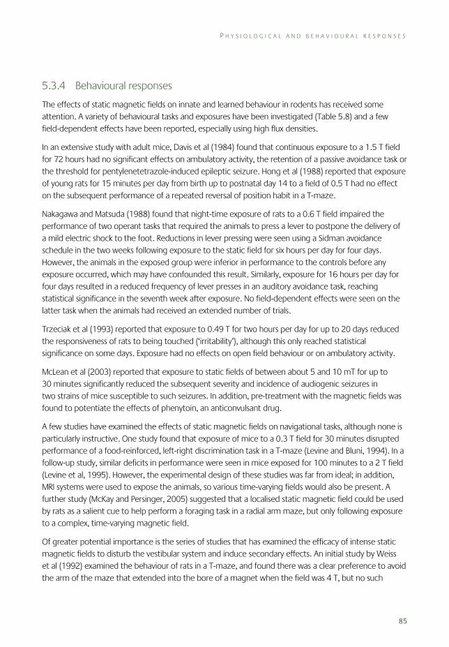
P H Y S I O L O G I C A L A N D B E H A V I O U R A L R E S P O N S E S
85
5.3.4 Behavioural responses
The effects of static magnetic fields on innate and learned behaviour in rodents has received some attention. A variety of behavioural tasks and exposures have been investigated (Table 5.8) and a few field-dependent effects have been reported, especially using high flux densities.
In an extensive study with adult mice, Davis et al (1984) found that continuous exposure to a 1.5 T field for 72 hours had no significant effects on ambulatory activity, the retention of a passive avoidance task or the threshold for pentylenetetrazole-induced epileptic seizure. Hong et al (1988) reported that exposure of young rats for 15 minutes per day from birth up to postnatal day 14 to a field of 0.5 T had no effect on the subsequent performance of a repeated reversal of position habit in a T-maze.
Nakagawa and Matsuda (1988) found that night-time exposure of rats to a 0.6 T field impaired the performance of two operant tasks that required the animals to press a lever to postpone the delivery of a mild electric shock to the foot. Reductions in lever pressing were seen using a Sidman avoidance schedule in the two weeks following exposure to the static field for six hours per day for four days. However, the animals in the exposed group were inferior in performance to the controls before any exposure occurred, which may have confounded this result. Similarly, exposure for 16 hours per day for four days resulted in a reduced frequency of lever presses in an auditory avoidance task, reaching statistical significance in the seventh week after exposure. No field-dependent effects were seen on the latter task when the animals had received an extended number of trials.
Trzeciak et al (1993) reported that exposure to 0.49 T for two hours per day for up to 20 days reduced the responsiveness of rats to being touched (‘irritability’), although this only reached statistical significance on some days. Exposure had no effects on open field behaviour or on ambulatory activity.
McLean et al (2003) reported that exposure to static fields of between about 5 and 10 mT for up to 30 minutes significantly reduced the subsequent severity and incidence of audiogenic seizures in two strains of mice susceptible to such seizures. In addition, pre-treatment with the magnetic fields was found to potentiate the effects of phenytoin, an anticonvulsant drug.
A few studies have examined the effects of static magnetic fields on navigational tasks, although none is particularly instructive. One study found that exposure of mice to a 0.3 T field for 30 minutes disrupted performance of a food-reinforced, left-right discrimination task in a T-maze (Levine and Bluni, 1994). In a follow-up study, similar deficits in performance were seen in mice exposed for 100 minutes to a 2 T field (Levine et al, 1995). However, the experimental design of these studies was far from ideal; in addition, MRI systems were used to expose the animals, so various time-varying fields would also be present. A further study (McKay and Persinger, 2005) suggested that a localised static magnetic field could be used by rats as a salient cue to help perform a foraging task in a radial arm maze, but only following exposure to a complex, time-varying magnetic field.
Of greater potential importance is the series of studies that has examined the efficacy of intense static magnetic fields to disturb the vestibular system and induce secondary effects. An initial study by Weiss et al (1992) examined the behaviour of rats in a T-maze, and found there was a clear preference to avoid the arm of the maze that extended into the bore of a magnet when the field was 4 T, but no such
5 A N I M A L S T U D I E S
86
preference existed using fields of 1.5 T. Thus it was suggested that the animals detected the presence of the field (or field gradients) and a strong aversive response had been induced. Recently these observations have been extended by Houpt et al (2007b). Female rats that had been trained to climb a vertical ladder for a food reward would only traverse the bore of an operating magnet on the first trial, and they would avoid entering an area where the field was greater than 2 T on subsequent trials. However, labyrinthectomised animals would readily enter and pass through a field of up to 14 T, suggesting that an intact peripheral vestibular apparatus was required for this learned response.
Using the conditioned taste aversion paradigm, Nolte et al (1998) reported that rats exposed to a 9.4 T field for 30 minutes reduced their intake of a highly palatable solution with a novel, sweet taste in a subsequent preference test with water. The aversive response was stronger, longer lasting, and gave better consistency between animals following multiple pairings between the solution and the field compared with a single pairing. In a follow-up study, it was found that a single pairing with a field of 14 T for at least one minute was sufficient to induce a reliable conditional taste response, and that the initial magnitude and persistence of the response depended on the intensity of the applied static field (Houpt et al, 2003). Investigating the sensory pathways in the rat brain stem associated with this conditioned response, Snyder et al (2000) reported that exposure for 30 minutes to a magnetic field resulted in increased c-Fos expression in several visceral nuclei, especially in the nucleus of the solitary tract and the lateral parabrachial nucleus, and in vestibular nuclei, such as the nucleus prepositus and nucleus supragenualis. This indicates that exposure was associated with increased neuronal activity within the brain stem. Previously, Messmer et al (1987) found that the pairing of a novel saccharine solution with a 30-minute exposure to the fields associated with MRI, including a 1.89 T magnetic field, produced no evidence of taste aversion, suggesting that a threshold may exist between 2 and 9 T for this response. Other MRI studies have reported that exposure to fields under 2 T appeared to have no effect on a variety of innate and learned behaviours in rodents (Innis et al, 1986; Ossenkopp et al, 1986).
In addition, Snyder et al (2000) noted that tight, circling locomotion could be transiently induced in animals following exposure to fields of 9.4 T, and it was suggested that such effects were consistent with the proposal of Schenck (2000, 2005) that small head movements in a large static field may induce vestibular stimulation through the action of magnetohydrodynamic forces on the fluid within the semicircular canals.
Houpt and colleagues have investigated this vestibular phenomenon further using fields of up to 14 T, various durations of exposure (1–30 minutes) and differing orientations of the animals within the field. In studies with restrained rats, Houpt et al (2003) found that the percentages of animals displaying tight circling activity was increased and rearing behaviour was suppressed for about one minute immediately upon release from restraint in a manner that depended on both the duration and intensity of exposure. There was evidence that the direction of circling depended on the animals’ orientation within the field: head-up exposure at 14 T for 30 minutes in a vertical field with the positive pole uppermost induced counterclockwise movements, and head-down exposure to the same field induced clockwise movements. However, it was not possible to determine whether this effect was attributable to the relative polarity of the field itself, or to the actual orientation of the animal, since the direction of the
P H Y S I O L O G I C A L A N D B E H A V I O U R A L R E S P O N S E S
87
field could not be reversed. In companion studies with restrained and unrestrained mice, Lockwood et al (2003) found that exposure to a 14 T field induced tight circling, reduced rearing, and produced a conditioned taste aversion to saccharine solution. With the exception of circling, unrestrained mice tended to exhibit larger effects than restrained mice, and it was suggested that movement during exposure may have enhanced the effects of the magnetic field. The neural basis of these responses was not investigated in either study, but the results suggested that the static fields had exerted an effect on components of the vestibulomotor system, and were thought to be consistent with the reports of vertigo and nausea in people working in strong magnetic fields (see Chapter 6).
Houpt et al (2005) extended these observations using fields of up to 19 T. It was found that tight circling behaviour was increased in rats after a single exposure to a field above 7 T, becoming significant at 17 T and above, and rearing was significantly reduced after exposures at 4 T. The direction of turning was found to correlate with the orientation of the animal relative to the magnetic field at 14 T: a resistive magnet was used that allowed the direction of the field to be reversed, so all animals could be exposed in the head-up orientation. Horizontal exposure of the animals, perpendicular to the field at 14 T, induced no effects on circling, but did significantly reduce rearing. Intake of saccharine solution was reduced using a single exposure to a field of 14 T and above, but repeated exposure to 4 T did not affect saccharine intake. Reversing the polarity of the field had little or no effect on the establishment or extinction of a conditioned taste aversion, and exposure of the animals perpendicular to the field at 14 T did not produce a conditioned response.
The same group (Cason et al, 2006) reported sex-related changes in the behavioural responses to magnetic fields. The incidence of field-induced circling caused by exposure to a 14 T field was found to be greater in female rats compared to males, and this was modulated by the level of oestrogen. Females also displayed a slower rate of extinction of the conditioned taste aversion than male rats, irrespective of oestrogen status.
More recently, the acute effects of static magnetic fields on drinking behaviour were examined in rats (Houpt et al, 2007c). Exposure to a 14.1 T field for 5–30 minutes was shown to increase significantly the latency to start drinking a palatable solution, and so decrease the amount of solution consumed. In addition, since exposure had no effect when the solution was delivered directly into the mouth using a catheter, it was concluded that the changes in drinking were mediated by effects on appetitive behaviours and not on consumatory actions (ie effects on activity and posture, and not on reflexes associated with drinking).
Lastly, the results of a study that varied exposure by altering the placement of animals within the bore of a magnet operated at a fixed flux density suggested that exposures of the head (and rostral body) are necessary for maximal behavioural changes (Houpt et al, 2007a). Further, the effects appeared to be unrelated to the field gradients experienced by the animals, or to transient passage through the field. Sex-related differences in response were also found.
Overall, this series of studies suggests that exposure to static magnetic fields above a threshold of between 4 and 7 T may induce immediate and delayed behavioural effects consistent with those seen after whole body rotation or other vestibular stimulation.
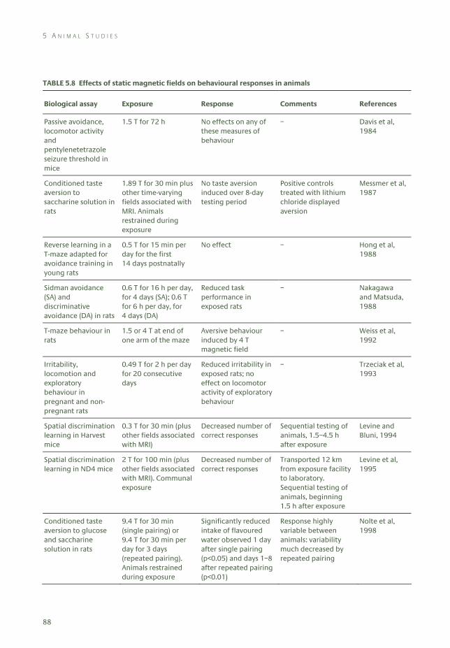
5 A N I M A L S T U D I E S
88
TABLE 5.8 Effects of static magnetic fields on behavioural responses in animals
Biological assay Exposure Response Comments References
Passive avoidance, locomotor activity and pentylenetetrazole seizure threshold in mice
1.5 T for 72 h No effects on any of these measures of behaviour
– Davis et al, 1984
Conditioned taste aversion to saccharine solution in rats
1.89 T for 30 min plus other time-varying fields associated with MRI. Animals restrained during exposure
No taste aversion induced over 8-day testing period
Positive controls treated with lithium chloride displayed aversion
Messmer et al, 1987
Reverse learning in a T-maze adapted for avoidance training in young rats
0.5 T for 15 min per day for the first 14 days postnatally
No effect – Hong et al, 1988
Sidman avoidance (SA) and discriminative avoidance (DA) in rats
0.6 T for 16 h per day, for 4 days (SA); 0.6 T for 6 h per day, for 4 days (DA)
Reduced task performance in exposed rats
– Nakagawa and Matsuda, 1988
T-maze behaviour in rats
1.5 or 4 T at end of one arm of the maze
Aversive behaviour induced by 4 T magnetic field
– Weiss et al, 1992
Irritability, locomotion and exploratory behaviour in pregnant and non-pregnant rats
0.49 T for 2 h per day for 20 consecutive days
Reduced irritability in exposed rats; no effect on locomotor activity of exploratory behaviour
– Trzeciak et al, 1993
Spatial discrimination learning in Harvest mice
0.3 T for 30 min (plus other fields associated with MRI)
Decreased number of correct responses
Sequential testing of animals, 1.5–4.5 h after exposure
Levine and Bluni, 1994
Spatial discrimination learning in ND4 mice
2 T for 100 min (plus other fields associated with MRI). Communal exposure
Decreased number of correct responses
Transported 12 km from exposure facility to laboratory. Sequential testing of animals, beginning 1.5 h after exposure
Levine et al, 1995
Conditioned taste aversion to glucose and saccharine solution in rats
9.4 T for 30 min (single pairing) or 9.4 T for 30 min per day for 3 days (repeated pairing). Animals restrained during exposure
Significantly reduced intake of flavoured water observed 1 day after single pairing (p<0.05) and days 1–8 after repeated pairing (p<0.01)
Response highly variable between animals: variability much decreased by repeated pairing
Nolte et al, 1998
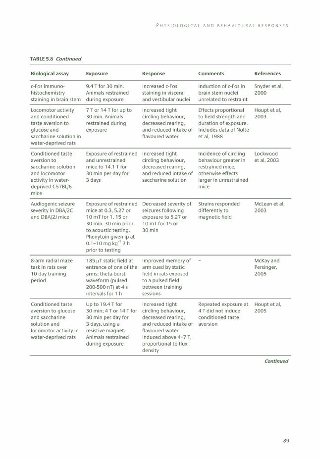
P H Y S I O L O G I C A L A N D B E H A V I O U R A L R E S P O N S E S
89
TABLE 5.8 Continued
Biological assay Exposure Response Comments References
c-Fos immuno-histochemistry staining in brain stem
9.4 T for 30 min. Animals restrained during exposure
Increased c-Fos staining in visceral and vestibular nuclei
Induction of c-Fos in brain stem nuclei unrelated to restraint
Snyder et al, 2000
Locomotor activity and conditioned taste aversion to glucose and saccharine solution in water-deprived rats
7 T or 14 T for up to 30 min. Animals restrained during exposure
Increased tight circling behaviour, decreased rearing, and reduced intake of flavoured water
Effects proportional to field strength and duration of exposure. Includes data of Nolte et al, 1988
Houpt et al, 2003
Conditioned taste aversion to saccharine solution and locomotor activity in water-deprived C57BL/6 mice
Exposure of restrained and unrestrained mice to 14.1 T for 30 min per day for 3 days
Increased tight circling behaviour, decreased rearing, and reduced intake of saccharine solution
Incidence of circling behaviour greater in restrained mice, otherwise effects larger in unrestrained mice
Lockwood et al, 2003
Audiogenic seizure severity in DBA/2C and DBA/2J mice
Exposure of restrained mice at 0.3, 5.27 or 10 mT for 1, 15 or 30 min. 30 min prior to acoustic testing. Phenytoin given ip at 0.1–10 mg kg–1 2 h prior to testing
Decreased severity of seizures following exposure to 5.27 or 10 mT for 15 or 30 min
Strains responded differently to magnetic field
McLean et al, 2003
8-arm radial maze task in rats over 10-day training period
185 μT static field at entrance of one of the arms; theta-burst waveform (pulsed 200-500 nT) at 4 s intervals for 1 h
Improved memory of arm cued by static field in rats exposed to a pulsed field between training sessions
– McKay and Persinger, 2005
Conditioned taste aversion to glucose and saccharine solution and locomotor activity in water-deprived rats
Up to 19.4 T for 30 min; 4 T or 14 T for 30 min per day for 3 days, using a resistive magnet. Animals restrained during exposure
Increased tight circling behaviour, decreased rearing, and reduced intake of flavoured water induced above 4–7 T, proportional to flux density
Repeated exposure at 4 T did not induce conditioned taste aversion
Houpt et al, 2005
Continued
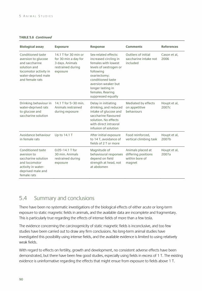
5 A N I M A L S T U D I E S
90
TABLE 5.8 Continued
Biological assay Exposure Response Comments References
Conditioned taste aversion to glucose and saccharine solution and locomotor activity in water-deprived male and female rats
14.1 T for 30 min or for 30 min a day for 3 days. Animals restrained during exposure
Sex-related effects: increased circling in females with lowest levels of oestrogen or following ovariectomy; conditioned taste aversion weaker but longer lasting in females. Rearing suppressed equally
Outliers of initial saccharine intake not included
Cason et al, 2006
Drinking behaviour in water-deprived rats to glucose and saccharine solution
14.1 T for 5–30 min. Animals restrained during exposure
Delay in initiating drinking, and reduced intake of glucose and saccharine flavoured solution. No effects with direct intraoral infusion of solution
Mediated by effects on appetitive behaviours
Houpt et al, 2007c
Avoidance behaviour in female rats
Up to 14.1 T After initial exposure to 14 T, avoidance of fields of 2 T or more
Food reinforced, vertical climbing task
Houpt et al, 2007b
Conditioned taste aversion to saccharine solution and locomotor activity in water-deprived male and female rats
0.05–14.1 T for 30 min. Animals restrained during exposure
Magnitude of behavioural responses depend on field strength at head, not at abdomen
Animals placed at differing positions within bore of magnet
Houpt et al, 2007a
5.4 Summary and conclusions
There have been no systematic investigations of the biological effects of either acute or long-term exposure to static magnetic fields in animals, and the available data are incomplete and fragmentary. This is particularly true regarding the effects of intense fields of more than a few tesla.
The evidence concerning the carcinogenicity of static magnetic fields is inconclusive, and too few studies have been carried out to draw any firm conclusions. No long-term animal studies have investigated this possibility using intense fields, and the available evidence is limited to using relatively weak fields.
With regard to effects on fertility, growth and development, no consistent adverse effects have been demonstrated, but there have been few good studies, especially using fields in excess of 1 T. The existing evidence is uninformative regarding the effects that might ensue from exposure to fields above 1 T.
R E F E R E N C E S
91
There are a number of reports of field-related effects on the cardiovascular system, most notably on arterial blood pressure and skin blood flow, often at fields much less than 1 T, which have not been independently corroborated. In addition, electric potentials generated across the aorta and other major arteries by the flow of blood in a static field can be routinely seen in the ECG of animals, including primates, exposed to fields in excess of 100 mT. However it is unclear whether there are any meaningful physiological consequences. The potential for strong fields to cause effects has not been explored in detail.
Studies investigating the effects of static magnetic fields on the nervous system have tended to use weak fields (of less than 1 T) and have produced variable, and sometimes conflicting, results. However, the possibility remains that exposure may influence electrophysiological response. A series of papers, mainly from one laboratory, indicates that exposure to static magnetic fields above a threshold of 4–7 T may induce behavioural and neural changes in animals. Animals exposed to these fields may experience an unpleasant vestibular disturbance consistent with self-reports by people after similar exposures.
5.5 References Bellossi A (1984). The effect of a static uniform magnetic field on mice a study of methylcholanthrene
carcinogenesis. Radiat Environ Biophys, 23, 107–9.
Bellossi A (1986a). The effect of a static non-uniform magnetic field on survival of leukaemia-prone AKR mice. Radiat Environ Biophys, 25, 75–80.
Bellossi A (1986b). The effect of a static non-uniform magnetic field on mice a study of Lewis tumour graft. Radiat Environ Biophys, 25, 231–4.
Bellossi A and Toujas L (1982). The effect of a static uniform magnetic field on mice. A study of a Lewis tumour graft. Radiat Environ Biophys, 20, 153–7.
Beischer DE (1969). Vectorcardiogram and aortic blood flow of squirrel monkeys (Saimiri sciureus) in a strong superconductive electromagnet. In Biological Effects of Magnetic Fields, Volume 2 (MF Barnothy, ed). New York, Plenum Press, pp 241–59.
Beischer DE and Knepton JC, Jr (1964). Influence of strong magnetic fields on the electrocardiogram of squirrel monkeys (Saimiri sciureus). Aerosp Med, 35, 939–44.
Bourland JD, Nyenhuis JA and Schaefer DJ (1999). Physiologic effects of intense MR imaging gradient fields. Neuroimaging Clin N Am, 9(2), 363–77.
Cason AM, Denbleyker M, Ferrence K, Smith JC and Houpt TA (2006). Sex and estrous cycle differences in the behavioral effects of high-strength static magnetic fields: role of ovarian steroids. Am J Physiol Regul Integr Comp Physiol, 290, R659–67.
Cavopol AV, Wamil AW, Holcomb RR, and McLean MJ (1995). Measurement and analysis of static magnetic fields that block action potentials in cultured neurons. Bioelectromagnetics, 16, 197–206.
Davis HP, Mizumori SYJ, Allen H, Rosenzweig MR, Bennett EL and Tenforde TS (1984). Behavioral studies with mice exposed to DC and 60-Hz magnetic fields. Bioelectromagnetics, 5, 147–64.
Gaffey CT and Tenforde TS (1981). Alterations in the rat electrocardiogram induced by stationary magnetic fields. Bioelectromagnetics, 1, 357–70.
Gaffey CT and Tenforde TS (1983). Bioelectric properties of frog sciatic nerves during exposure to stationary magnetic fields. Radiat Environ Biophys, 22, 61–73.
Gmitrov J and Ohkubo C (2002a). Artificial static and geomagnetic field interrelated impact on cardiovascular regulation. Bioelectromagnetics, 23, 329–38.
Gmitrov J and Ohkubo C (2002b). Verapamil protective effect on natural and artificial magnetic field cardiovascular impact. Bioelectromagnetics, 23, 531–41.

5 A N I M A L S T U D I E S
92
Gmitrov J, Ohkubo C and Okano H (2002). Effect of 0.25 T static field on microcirculation in rabbits. Bioelectromagnetics, 23, 224–9.
Gorgzynska E and Wegrzynowicz R (1991). Glucose homeostasis in rats exposed to magnetic fields. Invest Radiol, 26(12), 1095–100.
Grzesik J, Bortel M, Duda D, Kuska R, Ludyga K, Michnik J, Smolka B, Sowa B, Trzeciak H and Zielinski G (1988). Influence of a static magnetic field on the reproductive function, certain biochemical indices and behaviour of rats. Pol J Occup Med, 1(4), 329–39.
High WB, Sikora J, Ugurbil K and Garwood M (2000). Subchronic in vivo effects of a high static magnetic field (9.4 T) in rats. J Magn Reson Imaging, 12, 122–39.
Hinch R, Lindsay K, Noble D and Rosenburg JR (2005). The effects of static magnetic field on action potential propagation and excitation in nerve. Prog Biophys Mol Biol, 87(2–3), 321–8.
Hong C-Z, Harmon D and Yu B (1986). Static magnetic field influence on rat tail nerve function. Arch Phys Med Rehabil, 67, 746–9.
Hong C-Z, Huestis P, Thompson R and Yu J (1988). Learning ability of young rats is unaffected by repeated exposure to a static electromagnetic field in early life. Bioelectromagnetics, 9, 269–73.
Houpt TA, Pittman DW, Barranco JM, Brooks EH and Smith JC (2003). Behavioral effects of high-strength static magnetic fields on rats. J Neurosci, 23(4), 1489–505.
Houpt TA, Cassell JA, Riccardi C, Denbleyker A and Smith JC (2005). Behavioral effects on rats of high strength magnetic fields generated by a resistive electromagnet. Physiol Behav, 86, 379–89.
Houpt TA, Cassell JA, Cason AM, Riedell A, Golden GJ, Riccardi C and Smith JC (2007a). Evidence for a cephalic site of action of high magnetic fields on the behavioral responses of rats. Physiol Behav, 92(4), 665–74.
Houpt TA, Cassell JA, Riccardi C, DenBleyker MD, Hood A and Smith JC (2007b). Rats avoid high magnetic fields: dependence on an intact vestibular system. Physiol Behav, 92(4), 741–7.
Houpt TA, Cassell JA, Riccardi C, Kwon B and Smith JC (2007c). Suppression of drinking by exposure to a high-strength static magnetic field. Physiol Behav, 90, 59–65.
IARC (2002). Non-Ionising Radiation. Part 1: Static and Extremely Low Frequency (ELF) Electric and Magnetic Fields. IARC Monographs on the Evaluation of Carcinogenic Risks to Humans, Volume 80. Lyon, International Agency for Research on Cancer.
Ichioka S, Iwasaka M, Shibata M, Nakatsuka T, Harii K, Kamiya A and Ueno S (1998). Biological effects of static magnetic fields on the microcirculatory blood flow in vivo: a preliminary report. Med Biol Eng, 36, 91–5.
Ichioka S, Minegishi M, Iwasaka M, Shibata M, Nakatsuka T, Harii K, Kamiya A and Ueno S (2000). High intensity static magnetic fields modulate skin microcirculation and skin temperature in vivo. Bioelectromagnetics, 21, 183–8.
Ichioka S, Minegishi M, Iwasaka M, Shibata M, Nakatsuka T, Ando J and Ueno S (2003). Skin temperature changes induced by strong static magnetic field exposure. Bioelectromagnetics, 24, 380–86.
ICNIRP (1994). Guidelines on limits of exposure to static magnetic fields. Health Phys, 66(1), 100–106.
ICNIRP (1997). Biological effects of static and ELF electric and magnetic fields. In Proceedings of the International Seminar on Biological Effects of Static and ELF Electric and Magnetic Fields and Related Health Risks (R Matthes et al, eds), Bologna, Italy, June 1997. ICNIRP 4/97. München, Märkl-Druck.
ICNIRP (2003). Exposure to static and low frequency electromagnetic fields. In: Biological Effects and Health Consequences (0–100 kHz) (R Matthes et al, eds). ICNIRP 13/2003. München, Märkl-Druck.
Innis NK, Ossenkopp KP, Prato FS and Sestini E (1986). Behavioral effects of exposure to nuclear magnetic resonance imaging: II. Spatial memory tests. Magn Reson Imaging, 4, 281–4.
Itegin M, Günay I, Logoglu G and Isbir T (1995). Effects of static magnetic field on specific adenosine-5’-triphosphatase activities and bioelectrical and biomechanical properties in the rat diaphragm muscle. Bioelectromagnetics, 16, 147–51.
Jankovic BD, Maric D, Ranin J, and Veljic J (1991). Magnetic fields, brain and immunity: effects on humoral and cell-mediated immune responses. Int J Neurosci, 59(1–3), 25–43.
Jankovic BD, Jovanova-Nesic K, Nikolic V and Nikolic P (1993). Brain-applied magnetic fields and immune response: role of the pineal gland. Int J Neurosci, 70(1–2), 127–34.
R E F E R E N C E S
93
Jankovic BD, Nikolic P, Cupic V and Hladni K (1994). Potentiation of immune responsiveness in aging by static magnetic fields applied to the brain. Role of pineal gland. Ann NY Acad Sci, 719, 410–18.
Kangarlu A, Burgess RE, Zhu H, Nakayama T, Hamlin RL, Abduljalil AM and Robataille PML (1999). Cognitive, cardiac, and physiological safety studies in ultra high field magnetic resonance imaging. Magn Reson Imaging, 17, 1407–16.
Klimovskaya LD and Smirnova NP (1976). Change in the evoked potentials of the brain exposed to a constant magnetic field. Biull Eksp Biol Med, 82(8), 907–10.
Kloiber O, Okada Y and Hossmann K-A (1990). A 4.7 T static magnetic field has no effect on the electrical activity in the brain of cats. EEG EMG Z Elektoenzephalogr Electrmyogr Verwandte Geb, 21(4), 229–32.
Konermann G and Monig H (1986). Studies on the influence of static magnetic fields on prenatal development of mice. Radiologie, 26, 490–97.
Kowalczuk CI, Sienkiewicz ZJ and Saunders RD (1991). Biological effects of exposure to non-ionising electromagnetic fields and radiation. I. Static electric and magnetic fields. Chilton, NRPB-R238.
Kroeker G, Parkinson D, Vriend J and Peeling J (1996). Neurochemical effects of static magnetic field exposure. Surg Neurol, 45(1), 62–6.
Levine RL and Bluni TD (1994). Magnetic field effects on spatial discrimination learning in mice. Physiol Behav, 55, 465–7.
Levine RL, Dooley JK and Bluni TD (1995). Magnetic field effects on spatial discrimination and melatonin levels in mice. Physiol Behav, 58, 535–7.
Lockwood DR, Kwon B, Smith JC and Houpt TA (2003). Behavioural effects of static high magnetic fields on unrestrained and restrained mice. Physiol Behav, 78, 635–40.
McCann J, Dietrich F, Rafferty C and Martin A (1993). A critical review of the genotoxic potential of electric and magnetic fields. Mutat Res, 297, 61–95.
McLean MJ, Engström S, Holcomb RR, and Sanchez D (2003). A static magnetic field modulates severity of audiogenic seizures and anticonvulsant effects of phenytoin in DBA/2 mice. Epilepsy Res, 55, 105–16.
McLean MJ, Holcomb AW, Wamil AW and Pickett JD (1991). Effects of steady magnetic fields on action potentials of sensory neurons in vitro. Environ Med, 8, 36–45.
McLean MJ, Holcomb AW, Wamil AW, Pickett JD and Cavopol AV (1995). Blockade of sensory neuron action potentials by a static magnetic field in the 10 mT range. Bioelectromagnetics, 16, 20–32.
McKay BE and Persinger MA (2005). Complex magnetic fields enable static magnetic field cue use for rats in radial arm maze tasks. Int J Neurosci, 115, 625–48.
Messmer JM, Porter JH, Fatouros P, Prasad U and Weisberg M (1987). Exposure to magnetic resonance imaging does not produce taste aversion in rats. Physiol Behav, 40(2), 259–61.
Mevissen M, Stamm A, Buntenkötter S, Zwingleberg R, Wahnschaffe U and Löscher W (1993). Effects of magnetic fields on mammary tumour development induced by 7,12-dimethylbenz(a)anthracene in rats. Bioelectromagnetics, 14, 131–43.
Mevissen M, Butenkötter S and Löscher W (1994). Effects of static and time-varying (50-Hz) magnetic fields on reproduction and fetal development in rats. Teratology, 50, 229–37.
Mouritsen H and Ritz T (2005). Magnetoreception and its use in bird navigation. Curr Opin Neurobiol, 15(4), 406–14.
Morris C and Skalak T (2005). Static magnetic fields alter arteriolar tone in vivo. Bioelectromagnetics, 26, 1–9.
Murakami J, Torii Y and Masuda K (1992). Fetal development of mice following intrauterine exposure to a static magnetic field of 6.3 T. Magn Reson Imaging, 10, 433–437.
Nakagawa M (1984). Detection of electrophysiological responses in rabbits affected by short-term exposure to static magnetic field. Jap J Hyg, 38(6), 899–908.
Nakagawa M and Matsuda Y (1988). A strong static-magnetic field alters operant responding by rats. Bioelectromagnetics, 9, 25–37.
Narra VR, Howell RW, Goddu SM and Rao DV (1996). Effects of a 1.5-tesla static magnetic field on spermatogenesis and embryogenesis in mice. Invest Radiol, 31(9), 586–90.
Nolte CM, Pittman DW, Kalevitch B, Henderson R and Smith JC (1998). Magnetic field conditioned taste aversion in rats. Physiol Behav, 63(4), 683–8.
5 A N I M A L S T U D I E S
94
NRPB (2004). Review of the scientific evidence for limiting exposure to electromagnetic fields (0–300 GHz). Doc NRPB, 15(3), 1–215.
Ohkubo C and Xu S (1997). Acute effects of static magnetic fields on cutaneous microcirculation in rabbits. In Vivo, 11, 221–6.
Okano H and Ohkubo C (2001). Modulatory effects of static magnetic field on blood pressure in rabbits. Bioelectromagnetics, 22, 408–18.
Okano H and Ohkubo C (2003a). Anti-pressor effects of whole body exposure to static magnetic field on pharmacologically induced hypertension in conscious rabbits. Bioelectromagnetics, 24, 139–47.
Okano H and Ohkubo C (2003b). Effects of static magnetic fields on plasma levels of angiotensin II and aldosterone associated with arterial blood pressure in genetically hypertensive rats. Bioelectromagnetics, 24, 403–12.
Okano H and Ohkubo C (2005). Exposure to a moderate intensity static magnetic field enhances the hypotensive effect of a calcium channel blocker in spontaneously hypertensive rats. Bioelectromagnetics, 26, 611–23.
Okano H, Gmitrov J and Ohkubo C (1999). Biphasic effects of static magnetic fields on cutaneous microcirculation in rabbits. Bioelectromagnetics, 20, 161–71.
Okhano H, Masuda H and Ohkubo C (2005a). Effects of 25 mT static magnetic field on blood pressure in reserpine-induced hypotensive Wistar-Kyoto rats. Bioelectromagnetics, 26, 36–48.
Okano H, Masuda H and Ohkubo C (2005b). Decreased plasma levels of nitric oxide metabolites, angiotensin II, and aldosterone in spontaneously hypertensive rats exposed to 5 mT magnetic field. Bioelectromagnetics, 26, 161–72.
Okazaki R, Ootsuyama A, Uchida S and Norimura T (2001). Effects of a 4.7 T static magnetic field on fetal development in ICR mice. J Radiat Res (Tokyo), 42, 273–83.
Ossenkopp KP, Innis NK, Prato FS and Sestini E (1986). Behavioral effects of exposure to nuclear magnetic resonance imaging: I. Open-field behavior and passive avoidance learning in rats. Magn Reson Imaging, 4, 275–80.
Osuga T and Tatsuoka H (1999). Effect of 1.5 T steady magnetic field on neuroconduction of a bullfrog sciatic nerve in a partially active state within several hours after extraction. Magn Reson Imaging, 17(5), 791–4.
Reiter RJ (1993). Static and extremely low frequency electromagnetic field exposure: reported effects on the circadian production of melatonin. J Cell Biochem, 51(4), 394–403.
Repacholi MH and Greenebaum B (1999). Interaction of static and extremely low frequency electric and magnetic fields with living systems: health effects and research needs. Bioelectromagnetics, 20(3), 133–60.
Rosen AD (1992). Magnetic field influences on acetylcholine release at the neuromuscular junction. Am J Physiol, 262, C1418–22.
Rosen AD (1993). A proposed mechanism for the action of strong static magnetic fields on biomembranes. Int J Neurosci, 73, 115–19.
Rosen AD (1994). Thresholds and limits of magnetic field action at the presynaptic membrane. Biochim Biophys Acta, 1148, 317–20.
Rosen AD (1996). Inhibition of calcium channel activation in GH3 cells by static magnetic fields. Biochim Biophys Acta, 1282, 149–55.
Rosen AD (2003a). Mechanism of action of moderate-intensity static magnetic fields on biological systems. Cell Biochem Biophys, 39, 163–73.
Rosen AD (2003b). Effect of a 125 mT static magnetic field on the kinetics of voltage activated Na+ channels in GH3 cells. Bioelectromagnetics, 24, 517–23.
Rosen AD and Lubowsky J (1987). Magnetic field influence on central nervous system function. Exp Neurol, 95, 679–87.
Rosen AD and Lubowsky J (1990). Modification of spontaneous unit discharge in the lateral geniculate body by a magnetic field. Exp Neurol, 108, 261–5.
Saunders RD (2005). Static magnetic fields: animal studies. Prog Biophys Mol Biol, 87(2–3), 225–40.
Schenck JF (2000). Safety of strong, static magnetic fields. J Magn Reson Imaging, 12, 2–19.
Schenck JF (2005). Physical interactions of magnetic fields with living tissues. Prog Biophys Mol Biol, 87(2–3), 185–204.

R E F E R E N C E S
95
Schneider T, Thalau HP and Semm P (1994). Effects of light or different earth-strength magnetic fields on the nocturnal melatonin concentration in a migratory bird. Neurosci Lett, 168(1–2), 73–75.
Schwartz J-L (1978). Influence of a constant magnetic field on nervous tissues: I. Nerve conduction velocity studies. IEEE Trans Biomed Eng, BME 25, 467–73.
Schwartz J-L (1979). Influence of a constant magnetic field on nervous tissues: II. Voltage-clamp studies. Springfield VA, BME 26, 238–43.
Sikov MR, Mahlum DD, Montgomery LD and Decker JR (1979). Development of mice after intrauterine exposure to direct-current magnetic fields. In: Biological Effects of Extremely Low Frequency Electromagnetic Fields (RD Phillips et al, eds). 18th Hanford Life Sciences Symposium, Richland WA, October 1978. Springfield VA, US Department of Energy, National Technical Information Service, pp 462–73.
Smirnova NP, Klimovskaia LD and D’Iakonov A (1982). Significance of magnetic field parameters for altering brain evoked bioelectrical activity. Kosm Biol Aviakosm Med, 16(4), 61–3.
Snyder DJ, Jahng JW, Smith JC and Houpt TA (2000). c-Fos induction in visceral and vestibular nuclei of the rat brain stem by a 9.4 T magnetic field. NeuroReport, 11, 2681–5.
Sonnier H, Kolomytkin OV and Marino, AA (2000). Resting potential of excitable neuroblastoma cells in weak magnetic fields. Cell Mol Life Sci, 57(3), 514–20.
Sonnier H, Kolomytkin O and Marino AA (2003). Action potentials from human neuroblastoma cells in magnetic fields. Neurosci Lett, 337(3), 163–6.
Sutter BC, Billaydel B, Sutter-Dub MT and Bellossi A (1987). Effect of constant magnetic fields on the B-cells and insulin target cells in the rat. Aviat Space Environ Med, 58(6), 537–40.
Suzuki Y, Ikehata M, Nakamura K, Nishioka M, Asanuma K, Koana T and Shimizu H ()2001. Induction of micronuclei in mice exposed to static magnetic fields. Mutagenesis, 16(6), 499–501.
Tablado L, Perez-Sanchez F and Soler C (1996). Is sperm motility maturation affected by static magnetic fields? Environ Health Perspect, 104(11), 1212–16.
Tablado L, Perez-Sanchez F, Nunez J, Nunez M and Soler C (1998). Effects of exposure to static magnetic fields on the morphology and morphometry of mouse epididymal sperm. Bioelectromagnetics, 19(6), 377–83.
Tablado L, Soler C, Nunez M, Nunez J and Perez-Sanchez F (2000). Development of mouse testis and epididymis following intrauterine exposure to a static magnetic field. Bioelectromagnetics, 21(1), 19–24.
Tenforde TS (2005). Magnetically induced electric fields and currents in the circulatory system. Prog Biophys Mol Biol, 87(2–3), 278–7.
Tenforde TS, Gaffey CT, Moyer BR and Budinger TF (1983). Cardiovascular alterations in Macaca monkeys exposed to stationary magnetic fields: experimental observation and theoretical analysis. Bioelectromagnetics, 4, 1–9.
Tenforde T, Levy L and Vekerov E (1988). Biotelemetry recording of electrocardiographic indices and magnetically-induced blood flow potentials in rodents exposed to a 1.5-tesla static magnetic field. In: Abstracts of Tenth Annual Meeting of the Bioelectromagnetics Society. Stamford, Connecticut, June 1988. Paper A-07-5, p 13.
Togawa T, Okaim O and Oshima M (1967). Observation of blood flow EMF in externally applied strong magnetic fields by surface electrodes. Med Biol Eng, 5, 169–70.
Trabulsi R, Pawlowski B and Wieraszko A (1996). The influence of steady magnetic fields on the mouse hippocampal evoked potentials in vitro. Brain Res, 728, 135–9.
Trzeciak HI, Grzesik J, Bortel M, Kuśka R, Duda D, Michnik J and Malecki A (1993). Behavioral effects of long term exposure to magnetic fields in rats. Bioelectromagnetics, 14, 287–97.
Weiss J, Herrick RC, Taber KH, Contant C and Plishker GA (1992). Bio-effects of high magnetic fields: a study using a simple animal model. Magn Reson Imaging, 10, 689–94.
WHO (1987). Magnetic Fields. Environmental Health Criteria 69. Geneva, World Health Organization.
WHO (2006). Static Fields. Environmental Health Criteria 232. Geneva, World Health Organization.
Wieraszko A (2000). Dantrolene modulates the activity of steady magnetic fields on hippocampal evoked potentials in vitro. Bioelectromagnetics, 21, 175–82.
Wiltschko W and Wiltschko R (2005). Magnetic orientation and magnetoreception in birds and other animals. J Comp Physiol A Neuroethol Sens Neural Behav Physiol, 191(8), 675–93.

5 A N I M A L S T U D I E S
96
Withers HR, Mason KA and Davis CA (1985). MR effect on murine spermatogenesis. Radiology, 156(3), 741–2.
Xu S, Okano H and Ohkubo C (1998). Subchronic effects of static magnetic fields on cutaneous microcirculation in rabbits. In Vivo, 12, 383–90.
Xu S, Okano H and Ohkubo C (2000). Acute effects of whole-body exposure to static magnetic fields and 50 Hz electromagnetic fields on muscle and microcirculation in anaesthetised mice. Bioelectrochemistry, 53, 127–35.
Ye SR, Yang JW and Chen CM (2004). Effect of static magnetic fields on the amplitude of action potential in the lateral giant neuron of crayfish. Int J Radiat Biol, 80(10), 699–708.
Zimmermann B and Hentscheld D (1987). Effect of a static magnetic field (3.5 T) on reproductive behaviour of mice, on the embryo and fetal development and on selected hematologic parameters. Digitale Bilddiagn, 7(4), 155–61.
97
6 Human Exposures: Experimental Studies
6.1 Cardiovascular effects
Several mechanisms of action have been identified by which static magnetic field exposure may influence the human cardiovascular system. Direct mechanical torques on implanted intra-corporeal metallic and electrical devices, including replacement cardiac valves, artificial pacemakers and vascular stents, are potentially harmful and these risks are relatively well recognised but beyond the scope of this report. Cardiovascular effects that may result from direct exposure of biological tissues to static magnetic fields have received less attention. The most important effects are those that could influence normal human cardiovascular performance – for example, by altering rhythmic cardiac excitation, cardiac pump function, peripheral vascular resistance or organ perfusion. Relatively few human studies have attempted to measure or investigate these effects, although the animal studies and theoretical modelling described in earlier chapters have been used to identify and predict effects, particularly at fields above 2 T.
6.1.1 Mechanisms of action
6.1.1.1 Alteration of cellular function
As described in Chapter 4, static magnetic field effects have been demonstrated in vitro at a cellular level. Whilst it is difficult to extrapolate these observations to the functioning human cardiovascular system, changes of cellular function in vivo that influenced, for example, the slow depolarisation phase of potential changes in pacemaker tissues, contractility in cardiac or vascular myocytes, or the mechanical properties of blood would be expected to alter overall cardiovascular function.
6.1.1.2 Blood-flow-related induced electrical activity
Electric fields and therefore currents are induced when a conductor is moved in a static magnetic field (see Chapter 3). Although voluntary motion of part of the body such as a limb within a static magnetic field may induce such an electric field, the most important source of induced electric fields is flowing blood, and in humans the effect is maximal in the ascending aorta during systole. This occurs between the opening and closure of the aortic valve and during ventricular muscle repolarisation. As a result, the induced blood flow voltage is maximal at the same time as the normally induced voltage (observed as the ‘T’-wave in the human electrocardiogram or ECG). During clinical MRI examinations this results in ‘augmentation’ of the T-wave and is routinely observed in patients with ECG monitoring.
6 H U M A N E X P O S U R E S : E X P E R I M E N T A L S T U D I E S
98
Theoretically the induced blood flow voltage will also create leakage currents in the conducting tissues in and around blood vessels including the pacemaker and contractile tissues of the heart adjacent to the ascending aorta. As discussed in Chapter 3, theoretical modelling (Kinouchi et al, 1996; Holden, 2005) suggests that in the worst case with the aorta perpendicular to the magnetic field the induced current densities at 5 T are approximately 10% of the normal maximum endogenous cardiac current of approximately 1000 mA m−2 (Bernhardt, 1979; Holden, 2005); current densities of 1500 mA m−2 are estimated as the threshold for inducing ventricular fibrillation.
Although modelling has also estimated the likely magnitude of these currents in respect of other blood vessels and cardiac structures such as valves, there is little theoretical work estimating their effect on cardiovascular function – for example, through an effect on vascular resistance or valve function.
6.1.1.3 Magnetohydrodynamic effect
In Chapter 3 this mechanical effect and its likely cardiovascular impact in humans of reducing aortic blood flow was summarised. Both simple and detailed calculations of the effect suggest that without any compensation, and in the worst case (with the aorta perpendicular to the field, in contrast to most conventional MRI systems), aortic blood flow would be reduced by approximately 1% at 5 T, 5% at 10 T and 10% at 15 T (Kinouchi et al, 1996). This should be put in the context of the normal (sedentary) adult human whose cardiac output (flow) can increase to 500% of its resting value on exercise.
6.1.2 Human studies
The complex integrated nature of the human cardiovascular system, the many intrinsic and extrinsic factors that influence its performance, and the difficulty of making detailed and unbiased measurements within a magnetic field partly explain the relatively limited observations made in vivo. The majority have used well-known overall measures of performance such as heart rate and blood pressure to detect any effects and are summarised in Table 6.1.
6.1.2.1 Cardiac rhythm
Jehenson et al (1998) demonstrated a statistically significant (17%) increase in cardiac cycle length or RR interval after ten minutes of exposure to a 2 T static magnetic field in 12 healthy volunteers. This reverted to pre-exposure values in all subjects by ten minutes after removal of the field. Other studies (Shellock and Crues, 1987; Kangarlu et al,1999; Hinman, 2002; Chakeres et al, 2003), including three using higher magnetic fields, found no statistically significant alteration of heart rate or rhythm.
6.1.2.2 Cardiac pump function
No significant changes in blood pressure have been demonstrated with exposures of <100 mT (Hinman, 2002), 1.5 T (Shellock and Crues, 1987) and 8 T (Kangarlu et al, 1999). More recently, Chakeres et al (2003) monitored vital signs in a group of healthy volunteers; specifically the heart rate, respiratory rate, systolic and diastolic blood pressure, percutaneously estimated blood oxygenation and body temperatures by both external auditory canal measurements and sublingual measurements. Exposure to
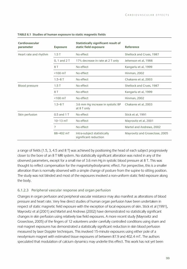
C A R D I O V A S C U L A R E F F E C T S
99
TABLE 6.1 Studies of human exposure to static magnetic fields
Cardiovascular parameter Exposure
Statistically significant result of static field exposure Reference
Heart rate and rhythm 1.5 T No effect Shellock and Crues, 1987
0, 1 and 2 T 17% decrease in rate at 2 T only Jehenson et al, 1988
8 T No effect Kangarlu et al, 1999
<100 mT No effect Hinman, 2002
1.5–8 T No effect Chakares et al, 2003
Blood pressure 1.5 T No effect Shellock and Crues, 1987
8 T No effect Kangarlu et al, 1999
<100 mT No effect Hinman, 2002
1.5–8 T 3.6 mm Hg increase in systolic BP at 8 T only
Chakares et al, 2003
Skin perfusion 0.5 and 1 T No effect Stick et al, 1991
10–13 mT No effect Mayrovitz et al, 2001
? No effect Martel and Andrews, 2002
88–402 mT Intra-subject statistically significant reduction
Mayrovitz and Groseclose, 2005
a range of fields (1.5, 3, 4.5 and 8 T) was achieved by positioning the head of each subject progressively closer to the bore of an 8 T MRI system. No statistically significant alteration was noted in any of the observed parameters, except for a small rise of 3.6 mm Hg in systolic blood pressure at 8 T. This was thought to reflect compensation for the magnetohydrodynamic effect. For perspective, this is a smaller alteration than is normally observed with a simple change of posture from the supine to sitting position. The study was not blinded and most of the exposures involved a non-uniform static field exposure along the body.
6.1.2.3 Peripheral vascular response and organ perfusion
Changes in organ perfusion and peripheral vascular resistance may also manifest as alterations of blood pressure and heart rate. Very few direct studies of human organ perfusion have been undertaken in respect of static magnetic field exposure with the exception of local exposures of skin. Stick et al (1991), Mayrovitz et al (2001) and Martel and Andrews (2002) have demonstrated no statistically significant changes in skin perfusion using relatively low field exposures. A more recent study (Mayrovitz and Groseclose, 2005) of the fingers of 12 volunteers under carefully controlled conditions using sham and real magnet exposures has demonstrated a statistically significant reduction in skin blood perfusion measured by laser Doppler techniques. This involved 15-minute exposures using either pole of a neodymium magnet with estimated tissue exposures of between 87.9 and 402.4 mT. The authors speculated that modulation of calcium dynamics may underlie this effect. This work has not yet been

6 H U M A N E X P O S U R E S : E X P E R I M E N T A L S T U D I E S
100
repeated elsewhere and the observed changes in perfusion are within the normal inter-subject variation of skin perfusion that would be observed in normal ambient environmental conditions.
6.1.3 Cardiovascular effects: summary
Static magnetic fields may theoretically affect the cardiovascular system by directly or indirectly influencing cellular function, cardiac rhythm, cardiac pump performance, vascular resistance and tissue perfusion.
Human studies of these effects are limited in their extent and methodology, particularly in the use of sham exposures and effective ‘blinding’ of both subjects and researchers. No detailed studies have been performed to identify the underlying mechanisms of the observed changes. No specific studies have been performed on subjects likely to be more vulnerable to cardiovascular effects of static magnetic fields.
Although local currents arising from induced voltage related to the ascending aorta blood flow have been identified as a potential influence on cardiac pacemaker function or myocardial contractility, no studies have directly measured such local currents or confidently identified a related effect in vivo.
In summary, for static magnetic fields of up to 8 T, limited human studies have demonstrated minimal cardiovascular effects that are well within the range of response of the normal cardiovascular system to normal daily environmental changes such as climate change or posture alteration.
6.2 Cognitive, neurological and sensory effects
Neurons transmit messages in the form of electrical impulses. This electrical activity is the basis of the brain’s sensory, motor and cognitive functions. Magnetic fields induce electric fields in nerve tissue. They could therefore cause neural activity, or interact with ongoing neural activity. When the body moves with respect to the magnetic field, additional effects could arise from induced eddy currents. Therefore, static magnetic fields could potentially influence the normal function of neurons, either peripherally in the body or centrally in the brain and spinal cord. Experimental studies of the effects of static magnetic fields on a range of human nervous system functions are reviewed here, including perception, motor control and higher cognitive functions such as memory.
Many studies have involved exposures that include both a static magnetic field and additional time-varying components, such as pulsed fields or field gradients. This report focuses on static fields; the effects of time-varying magnetic fields have been considered previously (AGNIR, 2001). However, when an exposure involves both a static field and additional time-varying components, such as arise with movement through the field, any effect of the exposure could potentially be due to either component. Therefore, this review covers a number of studies with combined exposures, since they could, in principle, reveal effects of static fields.
C O G N I T I V E , N E U R O L O G I C A L A N D S E N S O R Y E F F E C T S
101
Therapeutic trials of static magnetic fields for management of pain and neuropathy are reviewed separately in Chapter 7.
Experimental studies in humans can be classified according to the method used to study nervous system function. Nerve conduction studies have investigated whether magnetic fields alter the transmission of electrical impulses in peripheral nerves. Electroencephalographic (EEG) studies have investigated effects of magnetic fields on the spontaneous activity of networks of neurons in the resting brain. Evoked potential studies have studied magnetic field effects on the brain’s response to a sensory stimulus.
Most studies have compared a baseline measure of neural function obtained in the Earth’s ambient magnetic field with a repeated measure from the same test performed either during or shortly after exposure to an experimental magnetic field. Most studies focused on acute or very-short-term effects within a single exposure session. Few studies investigated the effects of repeated or lengthy exposures, and few involved long-term follow-up testing. Few of these studies explicitly stated whether they tested for and excluded possible interference from the field on the recording equipment itself, as opposed to on neural tissue. One study (de Vocht et al, 2006b) focused on occupational exposure rather than provocation, but used an experimental measurement approach, and is therefore reviewed here.
6.2.1 Nerve conduction studies
Hong (1987) measured the effects of static magnetic fields of 1 T on human motor nerve conduction. Briefly, electrodes were placed over the proximal portion of the arm or leg. Stimulating through these electrodes produces a contraction of the muscles in the distal part of the limb. The latency and amplitude of the contraction produced by a given electrical stimulus are used to measure the nerve’s conduction velocity and excitability, which are both key measures of neural transmission. A magnetic field was applied perpendicular to the limb using a small electromagnet in between the stimulating electrodes and the recording electrodes. Nerve conduction velocity and excitability were measured before the electromagnet was switched on and then after 5, 10 and 15 seconds of exposure. A further control measure was taken 3 minutes after the end of exposure to the magnetic field.
Nerve conduction velocity was not significantly altered by the magnetic field relative to the control values. However, nerve excitability was significantly increased above baseline values when the static field was present, at all three time points and in all three peripheral nerves studied. The temperatures of the electromagnet and the ambient environment were monitored and maintained at a constant level, so that the changes in nerve function could not be attributed to thermal effects. The author concluded that static magnetic fields increased human motor nerve excitability. Although the number of volunteers tested was low, the pattern of results appears quite consistent.
The mechanism underlying the effect is not clear. The author suggested that the effects may have depended on biological components with anisotropic magnetic susceptibilities (see Section 3.2.2). It seems unlikely, however, that these anisotropic susceptibilities would lead to detectable effects in fields of 1 T.

6 H U M A N E X P O S U R E S : E X P E R I M E N T A L S T U D I E S
102
Vogl et al (1991) investigated the effect of a clinical 1 T MRI scanner on nerve conduction velocity by measuring evoked potentials in 50 volunteers. The brain’s response to somatosensory or auditory stimuli was recorded using scalp electrodes. The authors also tested peripheral nerve conduction velocity by applying electrical stimuli over the ulnar nerve and measuring the contraction evoked in finger muscles. All tests were performed first in a control room. The measures were then repeated in the static magnetic field of the MRI scanner prior to the imaging protocol itself. The subjects then underwent a routine MRI examination for around one hour, during which they were exposed to radiofrequency pulses and pulsed magnetic field gradients, in addition to the static field. At the end of the imaging session the evoked potentials were again measured in the static magnetic field and finally the tests were repeated again in a control room. The authors stated that skin temperature was controlled throughout the experiment, although no thermal data were given.
The authors reported that the amplitude of the evoked potential could not be used to estimate neural excitability, because the recording equipment was influenced directly by the magnetic field. Instead, the timing of successive peaks of the evoked potentials was used as an index of transmission of the neural signal from the sensory receptors to the brain, and within the brain’s sensory pathways. No statistical analysis was presented, and the results were based on visual inspection of average data traces. No abnormalities in evoked potential waveforms or nerve conduction velocity were seen in any exposure condition. The interpretation of this study requires care because the results were not analysed statistically. However, the results suggest that static magnetic fields do not influence nerve conduction velocities.
6.2.2 Electroencephalographic (EEG) studies
Several studies have investigated the effects of magnetic fields on the human brain by measuring the electrical activity of the brain from scalp electrodes (the electroencephalogram or EEG). The EEG reveals the spontaneous synchronised firing of networks neurons. Changes in the amplitude or frequency spectrum of EEG patterns during or after exposure to static magnetic fields might indicate an effect of the field on brain function.
Von Klitzing (1989) recorded resting EEG in a 0.2 T whole body magnet while the magnetic field was either on or off. An increase in EEG power was noticed in the static magnetic field. However, no statistical analysis was performed, details of the data processing were not given, and it was not clear how many subjects participated in the experiment. Moreover EEG changes were more prominent in the right hemisphere of the brain than in the left hemisphere, for reasons that remain unexplained. These data would require replication and more formal analysis to constitute convincing evidence of an effect of static magnetic fields on the human EEG.
Dobson et al (2000a) investigated whether static magnetic fields could influence the patterns of brain activity in epileptic patients. Three patients who were being evaluated for abnormal EEG activity prior to neurosurgery underwent EEG recording from intracranial and scalp electrodes while wearing a customised helmet that generated static magnetic fields of 0.9–1.8 mT. The EEG measured in the static magnetic field was compared to the EEG measured during a control period immediately beforehand,

C O G N I T I V E , N E U R O L O G I C A L A N D S E N S O R Y E F F E C T S
103
when only the Earth’s ambient field was present. During the experimental sessions the magnetic field was switched on and off repeatedly, at intervals varying from 2–40 seconds depending on the protocol used. In two patients the presence of the magnetic field was associated with an increase in interictal epileptiform spiking (the abnormal EEG activity characteristic of epilepsy). In the third patient, cycling of the magnetic field abolished the same abnormal pattern of spiking.
The authors concluded that time-dependent changes in magnetic fields could influence the EEG patterns. However, there was no formal attempt to distinguish the effects of the static magnetic field from those of time-varying fields. The mechanism underlying the effects was not identified, and no explanation was offered for the inconsistency between individuals in the direction of EEG changes. Moreover, the implications for brain function in non-epileptic healthy volunteers are unclear.
Dobson et al (2000b) recorded the EEG from ten patients with middle temporal lobe epilepsy using similar methods to those of the previous study. A standardised exposure protocol was used, comprising a control period with the Earth’s ambient magnetic field only, followed by exposures to fields of 1, 2, 3 and 4 mT. Within each exposure period, the static field was repeatedly switched on and off, with a controlled cycle period. Care was taken to ensure that the patients did not know whether the magnetic field was on or off. The dependent variable was the number of epileptiform spikes in the EEG. Over the experiment as a whole, the number of abnormal spikes did not differ significantly between control periods and periods when the magnetic field was applied. Inspection of the data for individual subjects, however, indicated differences in abnormal spike activity between exposed and control conditions in half the patients. In some cases the abnormal spike activity increased during application of the field and in some cases it decreased. No data were given for the different magnetic flux densities so it is unclear whether a dose–response relationship exists or not. There was no formal attempt to distinguish the effects of the static field from the effects of switching the field on and off. In summary, the effects found in this study were not systematic, and may be linked to time-varying rather than static magnetic fields. In addition, the outcome measure was an index of epileptiform activity in patients with epilepsy. Therefore, the implications for function of the healthy brain, and for the wider population, remain unclear.
Fuller et al (1995) used a similar method to that of the previous study. Six patients with epilepsy were studied. Fields of 0.9, 1.3 or 1.8 mT were applied for 20 seconds followed by 40 seconds with the field off, and the number of interictal epileptiform EEG spikes was counted. Although no statistical analysis was given, the results showed more frequent EEG spikes during exposure to a magnetic field than during control periods.
Taken together, the previous three studies suggest that relatively weak magnetic fields can influence the epileptic brain. However, the effect appears to involve time-varying rather than static fields. The direction of the effect is inconsistent: magnetic fields promoted abnormal EEG activity in some patients and suppressed it in others. No plausible mechanism is suggested to account for this inconsistency. Moreover, these studies have all been performed within a single laboratory, using small numbers of patients with abnormal patterns of brain activity. It remains unclear whether comparable effects occur in the healthy brain, and whether the static magnetic field, as opposed to time-varying fields, could be responsible.
6 H U M A N E X P O S U R E S : E X P E R I M E N T A L S T U D I E S
104
6.2.3 Evoked potential studies
Hotz et al (1992) investigated the effect of a typical clinical MRI exposure on auditory brain stem responses (ABRs). The latencies of ABR waves are an important measure of neural transmission within the brain. The ABRs of 11 subjects were measured before and immediately after a 1.5 T MRI scan lasting 50 minutes. No significant changes in ABR latency were found. The authors concluded that routine MRI examination did not induce changes in neural transmission within the auditory system.
In an earlier study, Müller and Hotz (1990) used an apparently identical design to the Hotz et al (1992) study. The ABRs were measured before and after exposure to magnetic fields during a routine MRI scan using a 1.5 T scanner. Again, no significant effect of MRI exposure on ABR latency was found.
Hong and Shellock (1990) measured the latency and amplitude of the somatosensory evoked potentials (SEP). In this test, an electrical stimulus is applied to the skin, and brain activity in response to the stimulus is recorded from electrodes on the scalp. The latency and amplitude of the response are established measures of neural transmission. Eleven volunteers underwent SEP recordings in a pre-exposure baseline condition when only the Earth’s ambient magnetic field was present, and while lying in a commercial MRI scanner having a 1.5 T static magnetic field. The scanner was not operating at the time of testing, and so only the static magnetic field was present. Two key SEP waves were measured. Neither the latency nor the amplitudes of these SEP components changed between pre-test and exposure conditions. The authors concluded that acute exposure to a static magnetic field did not influence either the speed of neural transmission or the cerebral cortical activity evoked by sensory stimulation.
Vogl et al (1991) included both an evoked potential and a nerve conduction velocity component. Both components have been discussed together in the previous section.
Winther et al (1999) studied the effects of prolonged exposure to weak static magnetic fields on acoustic and vestibular functions of the inner ear. Eleven medical student volunteers were exposed during one night of sleep next to a 0.5 T MRI unit. Only the static magnetic field was present, and no RF signals or gradient pulses were applied. The field in the location where the subjects slept was said to be between 2 and 7 mT. Seven standard tests of acoustic and vestibular function were performed before and immediately after nine hours of exposure during sleep. The tests included thresholds for hearing pure tone signals, a speech recognition task, measures of oto-acoustic emissions, ABR evoked responses and oculomotor nystagmus elicited by caloric vestibular stimulation. These tests are all known to be sensitive to the physiological condition of the inner ear. No significant differences were found between performance before and after exposure to the static field, on any of the seven tests. The authors concluded that exposure to static magnetic fields between 2 and 7 mT for nine hours did not affect the acoustic or vestibular functions of the inner ear.
6.2.4 Cognitive studies
A study by Brockway and Green (1992) was motivated by anecdotal reports from some patients and health professionals of feeling dazed, confused or unable to retrieve words from memory following routine MRI examinations. The authors performed a variety of memory tests before and after MRI
C O G N I T I V E , N E U R O L O G I C A L A N D S E N S O R Y E F F E C T S
105
examinations of 421 participants, who were either patients undergoing routine clinical MRI or healthy volunteers. The cognitive measures studied included the ability to recognise and recall faces, names for objects, words and sequences of numbers (the ‘digit span’ test). The exposures involved a variety of routine MRI sequences for imaging various body parts. Several separate experiments were reported. Study 4 of the series had the most appropriate and informative experimental design. In this, 71 participants were shown pictures of faces and common objects and were then asked to recall these. Digit span was also tested. The tests were performed both before and after routine MRI scanning. A further 42 subjects served as a ‘sham MRI control’ group. They performed the same memory tests before and after lying in a wooden tube designed to simulate the physical and sensory environment of an MRI scanner without static or pulsed gradient magnetic fields or RF exposure. The control subjects listened to a tape-recording of the sounds generated by a typical MRI session during the sham exposure. Recall performance typically deteriorated between pre-test and post-test, while digit span improved. However, these changes were seen in both the MRI-exposed group and in the sham-exposed control group. There was no statistically significant evidence for greater changes in memory performance in the exposed group than in the control group. The authors concluded that MRI did not cause loss of memory. They suggested that anecdotally-reported effects of MRI on memory may have been due to the stressful and unusual sensory environment of the MRI scanner.
Besson et al (1984) performed a variety of cognitive tests both before and after MRI exposure in seven healthy volunteers. The static magnetic field was weak (0.04 T) compared to modern MRI exposures, and exposure lasted only ten minutes. Two imaging sessions were carried out, separated by an average interval of four months. The authors compared subjects’ performance on cognitive tests carried out before the first imaging session with that on repeat testing after the second session. The cognitive tests included standard intelligence, memory and word fluency tests, and a ‘Stroop’ test of executive function. No evidence of any adverse effect of MRI on cognitive performance was found. There was a statistically significant improvement in scores on the intelligence test. However, this was attributed to practice rather than to the exposures associated with MRI. The authors concluded that exposure to the magnetic fields associated with MRI had no enduring effect on cognitive functions including memory, at least for these weak fields.
Sweetland et al (1987) randomly allocated 157 healthy volunteers to one of three exposure groups. Those in an ‘imaged’ group were exposed for approximately one hour to a routine MRI sequence in a 0.15 T clinical scanner. A sham-exposed group lay in the MRI scanner with all magnetic fields, including the static field of the resistive magnet, switched off, and listened to audio recordings of the sounds generated in MRI examinations. A control group spent a similar period of time in a waiting area outside the field of the MRI machine. Each subject was tested using a cognitive test battery before exposure, immediately after exposure and in a follow-up test three months later. The test battery included intelligence measures (digit span, block design and digit symbol), memory for lists of paired associates, and measures of visual working memory and visuo-spatial transformations. A measure of state anxiety (ie current anxiety levels) was also taken. The psychologist administering the tests was blind as to the exposure condition.
The results showed only two significant differences between the exposed group and the sham-exposed group. The exposed group had poorer performance on digit span memory than the sham group
6 H U M A N E X P O S U R E S : E X P E R I M E N T A L S T U D I E S
106
immediately after exposure. The exposed group had higher anxiety levels than the sham-exposed group at the three month follow-up. Inspection of the published data suggests, however, that this result arose because of differences between the groups at pre-test and at follow-up. Anxiety levels in the exposed group actually decreased between pre-test and post-test, suggesting that acute exposure did not increase anxiety. The authors suggested that these significant results could have been due to chance, given the large number of statistical tests performed. Subsequent studies of memory using the same test materials and much stronger fields have failed to find memory impairments following MRI exposure (Chakeres et al, 2003b).
In their 2003 study, Chakeres and colleagues compared the performance of 25 subjects on a battery of cognitive tests in two magnetic field conditions: lying inside the bore of an 8 T research MRI scanner or away from the magnet in the same room where the magnetic field was 0.05 T. The scanner’s RF and gradient switching coils were inactive in both conditions, leaving the strength of the static magnetic field as the key difference between the two exposure conditions. The order of conditions was randomised and counterbalanced. Subjects performed a number of established neuropsychological cognitive tests in each exposure condition. The tests included reaction times, a digit span test involving retaining lists of numbers in short-term memory, and memory for word lists. Different versions of the tests were given each time they were administered, to prevent learning effects. Overall, cognitive performance was generally better at 8 T than at 0.05 T, although this difference was not significant for any test. On one test of word recognition, performance was significantly worse in the 8 T field than at 0.05 T. The authors attributed this to chance, and pointed out that the size of this difference was small and not clinically meaningful. The authors concluded that static magnetic fields as high as 8 T had no acute effect on cognitive performance. Subjects were questioned (but not re-tested) at a three-month follow-up. None reported adverse effects.
The authors themselves noted some limitations of this study. First, the physical environment differed between the two conditions, not only in the static magnetic field but also in sensory stimulation. The bore of an MRI magnet is an unusually restricted visual environment, which might of itself impair cognitive function. However, the authors argued that the combination of the static magnetic field and reduced visual environment in the MRI scanner did not reliably affect cognitive function, compared with testing outside the scanner. They therefore suggested that magnetic field effects alone would also be ineffective, although they did not consider that the two effects might be antagonistic. Second, the authors measured cognitive performance in a single session, whose duration was not stated. They could not therefore exclude the possibility of delayed effects on cognitive function, but they noted that their subjects reported no adverse effects at the three-month follow-up.
A study by Kangarlu et al (1999) primarily focused on the effects of an 8 T static magnetic field on physiological function in pigs and humans. Those results are discussed elsewhere in this report (see Section 6.1). The same authors additionally performed limited cognitive testing on the human subjects (volunteers), which is reviewed here. Ten individuals initially performed the Mini Mental State Examination, to provide a basic assessment of cognitive function. Participants also performed a verbal fluency task and a peg-placing task sensitive to executive use of language and to motor function, respectively. Each subject was then placed in the static magnetic field of an 8 T MRI machine for one hour and performed the tests again immediately on removal. No RF pulses or gradient
C O G N I T I V E , N E U R O L O G I C A L A N D S E N S O R Y E F F E C T S
107
switching were applied, so that any effects found could be attributed to the static field only. No statistically significant differences were found between pre- and post-exposure conditions in any of the measures studied.
The authors concluded that exposure for one hour to an 8 T field had no significant acute effect on these basic clinical measures of cognitive function. One possible criticism of this study relates to the cognitive measures used. The tests selected are generally used for describing deficits in patients with brain diseases, and may be insufficiently sensitive to detect small changes in cognitive function in healthy people. For example, performance on the Mini Mental State Examination appeared to be almost at ceiling in both conditions.
De Vocht et al (2003) focused on the possible effects of occupational exposure to magnetic fields in professionals working in MRI facilities. Seventeen people working for a MRI equipment manufacturing company performed a variety of cognitive motor and sensory tests in two exposure conditions, either with or without the presence of a 1.5 T magnetic field generated by a conventional MRI scanner. Importantly, the subjects did not lie in the bore of the scanner but sat outside it at the approximate location of a surgical team using operating theatre MRI equipment. At this position, the static field was measured as 0.7 T, and the field’s spatial gradient (dB/dz , see Chapter 3) was maximal. An additional factor in the experimental design was the performance of manual movements designed to simulate the movements of a surgeon during a surgical procedure. These movements consisted of placing an object in the magnet bore and removing it at approximately ten-second intervals. These movements were included because movement through a static field would generate gradient fields within the subject. Actual exposure was measured using a magnetometer affixed to each subject’s head.
The four conditions tested therefore were: magnetic field off, no additional movements; magnetic field off, subjects performed additional movements; magnetic field on, subjects performed additional movements; magnetic field on, subjects did not perform additional movements. Subjects were exposed to these conditions in a fixed sequence in four separate one-hour testing sessions spaced at one-week intervals.
A battery of cognitive and motor tests was delivered in a fixed order during each one-hour session. In conditions where subjects made additional movements, the cognitive testing was interleaved with four-minute blocks of manual movements. The cognitive tests were standard measures of cognitive and motor function widely used in psychometric assessment and environmental health settings. They included peg-moving and pursuit manual tracking tests sensitive to motor coordination, a digit-span task involving short-term memory for lists of numbers, visual search and visuo-motor attention tests, a Stroop test of executive function, and perceptual tests of visual contrast sensitivity at several spatial frequencies.
De Vocht et al gave data for mean performance on each test with the magnetic field on and off. Since all subjects performed the tests several times, and since the field exposures were performed in a fixed sequence, comparisons between field-on and field-off conditions also included effects of time and learning. The authors attempted to remove the learning effect using a statistical modelling technique, and tested for a significant effect of magnetic field exposure after accounting for the learning effect. The raw, unadjusted data were not given. Data were not shown separately for conditions with and without additional movements, although the authors stated that additional movements had no effect.
6 H U M A N E X P O S U R E S : E X P E R I M E N T A L S T U D I E S
108
Digit span, visual search, Stroop and peg-moving tasks showed no significant effects of magnetic field exposure. Exposure to the magnetic field was associated with a significant decrease of 3.9% in accuracy on a manual tracking task. However, this result should be interpreted with caution because the speed of performance on the same task was greater when exposed to the magnetic field than when not exposed. Speed and accuracy in cognitive and motor tasks such as tracking are generally related by a reciprocal trade-off function – that is, greater accuracy can often be achieved by decreasing speed. Participants may have chosen to emphasise speed rather than accuracy in the magnet-on condition, but not in the magnet-off condition. Therefore, the change in tracking accuracy with flux density may not indicate an actual change in cognitive processing.
De Vocht et al also found decreases in visual contrast sensitivity in the magnet-on condition. These changes were significant for the lower spatial frequencies tested (1.5 and 3 cycles per degree) but non-significant trends in the same direction were seen for other spatial frequencies as well. In interpreting the data no account was taken of the multiple comparisons between the different spatial frequencies tested, either within the visual contrast sensitivity tests or for the family of tests as a whole. Appropriate adjustment of the level of statistical significance for multiple comparisons might render some of these changes non-significant.
The authors concluded that exposure to a static magnetic field, such as that at the entry to the bore of an operating MRI scanner, could have significant neurobehavioural effects. They further suggested that these could adversely impact on the level of performance of a worker such as a surgeon.
The apparent effects on motor performance in this study should be interpreted with caution, because the authors failed to consider the effects of speed–accuracy trade off. The effects on visual contrast sensitivity carry greater weight, although some correction of the results for multiple comparisons may be required. More generally, the overall experimental design of the study is problematic, because differences in exposure between the four conditions are confounded with effects of learning and passage of time. The visual contrast sensitivity tests should be repeated in a counterbalanced design, with appropriate statistical correction for multiple comparisons, to assess whether these effects are due to the static magnetic field exposure.
De Vocht et al (2006a) investigated the relation between the static magnetic field and a battery of neurobehavioural tests and symptoms. Twenty volunteers sat just outside the bore of 3 and 1.5 T scanners or in a control location with exposure to only the Earth’s ambient field. The effective flux densities at the location of each subject’s head were estimated at 1 T and 600 mT, respectively, for the two scanners. RF and pulsed gradient fields were not present. Subjects made horizontal head movements at 0.4 m s–1 to track a moving target either just before or during performance of the tests. Such movements would expose the subject to a time-dependent field, but the actual dB/dt values of this exposure are not given. Tests of working memory, eye–hand coordination and visual perception were administered over a 30-minute period, with 20-second periods of head movement interleaved between successive elements in the test battery. All subjects participated in pre-tests to minimise learning effects. They then performed the tests in the 3 T, 1.5 T and control exposure conditions in fixed order, with a three-week interval between each condition.
C O G N I T I V E , N E U R O L O G I C A L A N D S E N S O R Y E F F E C T S
109
Scores on visual and auditory working memory, visual tracking performance, and speed (but not precision) of performing an eye–hand coordination task differed across the three field conditions. Specifically, there were small decrements in performance when exposed to static magnetic fields, compared with the control condition. These decrements were typically less than 1%, and were largest for visual tracking (3.1% decrement). Performance on a visual contrast sensitivity task that the same researchers had previously found to be affected by static magnetic fields (de Vocht et al, 2003) was not affected in this study.
A major concern with this study is the potential for confounding by learning and practice effects. All subjects performed in the 3 T field first, followed by the 1.5 T field and then the control session. Performance on most behavioural and cognitive tests improves strongly with practice. In this study, practice effects and magnetic field effects are completely confounded. The authors suggested that the presence of pre-test, and the relatively long interval between each testing session, should have minimised learning effects, but offered no independent evidence to support this view. This study should be repeated using a counterbalanced design, in which different groups of subjects are exposed to all fields in all possible orders, so that the field effects can be separated from learning effects. Finally, as the authors themselves noted, the effects in this study may have been too small to have any important impact on psychomotor performance of the target group (healthcare workers exposed during interventional MRI).
De Vocht et al (2007) investigated the effects of stray fields from a 7 T magnet on cognitive function in 27 healthy volunteers. Each subject performed a cognitive test battery in three exposure conditions, corresponding to three different positions relative to the bore of an MRI scanner. No RF pulses or switched gradient fields were present. The fields in each condition were designed to be 1600 mT (high exposure), 800 mT (medium exposure) and 2 mT (negligible exposure). The high exposure condition was repeated twice. In one session, the subjects performed additional head movements to look at one of four lights on a horizontal bar illuminated in turn. This required a range of head movement of around 90° and a movement frequency of around 0.625 Hz. Ten cycles of head movements were made prior to each cognitive test. The authors reported that in the high exposure condition, the volunteer’s head might experience exposures within a range from 500 mT to 2 T, according to variations in head position as the head movements and the tasks in the test battery were performed. A further high exposure session did not require such movements.
The order of exposure conditions was randomised for each subject. The volunteers were blinded as to the actual exposure condition, by being led blindfold from a waiting area into an enclosed tent where the blindfold was removed prior to testing.
The cognitive battery was similar to that used in previous studies (de Vocht et al, 2006a), and comprised tests of eye–hand coordination, recall of digits and letters from memory, auditory working memory (N-back task), visual perception (contrast sensitivity), visuo-spatial processing (line bisection), and visual tracking (following entangled lines on paper and marking where they ended). Subjects received a different version of the tests in each session.
Statistical results showed significant differences between exposure levels in the visual tracking task. Tracking speed was fastest in the negligible exposure condition, slower in the medium exposure, and
6 H U M A N E X P O S U R E S : E X P E R I M E N T A L S T U D I E S
110
slower still in the high exposure condition. Differences between exposure conditions on the eye–hand coordination and line-bisection tasks showed a trend towards significance. However, comparison of the speed and accuracy scores on these tests suggests the effects reflect changes between exposure conditions in speed–accuracy trade off rather than changes in underlying information-processing capacity.
Additional statistical tests compared high exposure conditions with and without additional head movements. These showed a trend for head movements to impair performance in the eye–hand coordination task, and the visual tracking task. An effect was also found for the contrast sensitivity test of visual perception, but only at one of five spatial frequencies tested.
The most prominent result of this study is the impairment of visual tracking performance with increasing strength of the magnetic field. This replicates previous reports of impairments in tracking near the bore of 1.5 and 3 T scanners (de Vocht et al, 2006a), although the effects reported in the present study are numerically smaller. The authors concluded that visual sensory processing and eye–hand coordination may have been affected by stray fields from MRI scanners, and that the dynamic field component caused by the interaction between movement of the subject and the static magnetic field was more important than the static field in itself. The authors suggested that static fields may have interfered with the vestibulo-ocular mechanisms responsible for stability of gaze, but did not interfere with cognitive processes directly.
However, repeated head movements could impair visual tracking performance even in the absence of any interaction with static magnetic fields – for example, by inducing dizziness, loss of spatial orientation, or adaptation of vestibulo-ocular control mechanisms. The study did not include a baseline condition without movements and also without field exposure. Therefore, a study of this design cannot be used to determine whether the impairment when movements are made in a strong field is due simply to making movements, or due to an interaction between the movements and the field. An experimental design which independently manipulated the factors of movements (present, absent) and static field (present, absent) could resolve this issue.
6.2.5 Brain metabolism studies
Volkow et al (2000) investigated the effects of a 4 T static magnetic field on the metabolic activity of the brain. The uptake of glucose by the brain depends on the level of ongoing neural activity. Therefore, any change in brain metabolic activity during exposure to a static magnetic field could reflect a direct effect of the field on neural activity, and potentially on brain function. The authors administered a radioactively-labelled form of glucose (18FDG) to 12 volunteers, exposed them to three different magnetic field conditions, and measured the uptake of 18FDG by the brain 50 minutes later using a PET scanner. The 18FDG PET measurements mostly reflected brain metabolic activity during the 35-minute period immediately following the injection, and prior to the PET measurements. Thus, PET data could reveal any differences in brain activity due to the magnetic fields that the subjects experienced in the delay interval between injection of the tracer and the PET measurement. Three magnetic field conditions were tested. In the first condition, subjects lay in the PET scanner during the delay interval and were exposed only to the Earth’s ambient magnetic field. In the second condition, subjects lay in a 4 T MRI
C O G N I T I V E , N E U R O L O G I C A L A N D S E N S O R Y E F F E C T S
111
scanner during the delay interval. In addition to the static magnetic field of the MRI scanner, a gradient echo sequence was applied to simulate routine MRI examinations, but RF exposure was disabled. The third condition was a sham MRI exposure which aimed to duplicate the sensory environment of the MRI scanner with no magnetic fields. The sham-exposure condition was achieved in a PET scanner by enclosing the subject’s head in the conventional MRI head cage and placing the subject within a cylindrical tube designed to mimic the enclosed visual environment of an MRI scanner bore. Thus, in the sham-exposure condition the subjects had identical visual experience to normal MRI but no magnetic field exposure above ambient levels. Sham MRI exposure also lacked the acoustic stimulation of the true MRI condition.
Results were analysed to identify possible differences between exposure conditions in metabolic activity of ten key brain regions. No significant differences in brain metabolic activity between the real and sham MRI environments were found in eight of the ten brain areas. Metabolic activity in the thalamus and cerebellum was significantly higher in the real MRI exposure than in the sham-exposure condition. However, this difference cannot be unambiguously attributed to the presence of the magnetic fields in the real MRI exposure condition because brain metabolic activity was also higher in the PET condition than in the sham-exposure condition, yet subjects were not exposed to any additional magnetic field in the PET condition. Instead, Volkow et al attributed the pattern of their results to an order effect: the subjects performed the sham-exposure condition last in the experimental sequence and were therefore more fatigued than for the previous two conditions. This study would need to be replicated with a counterbalanced design controlling for order effects before any clear conclusions about the effects of magnetic fields on brain metabolism or brain activity could be drawn.
6.2.6 Acute primary sensory effects
Several studies have reported that exposure to MRI-type signals can directly stimulate the nervous system. People undergoing MRI procedures in high field scanners have reported vertigo (sensations of dizziness), illusory visual experiences (magnetophosphenes), ringing sensations in the head, and metallic tastes in the mouth.
Vertigo is the most salient and best researched of these acute sensory effects. It is thought to arise from direct effects of the magnetic field on the vestibular organs, and from magnetohydrodynamic effects in the fluid of the semicircular canals. A recent review of motion sickness has been given by Golding (2006). The review includes a discussion of the predictors of individual susceptibility and the various countermeasures that can be used to reduce symptoms, both of which might be relevant to magnetic-field-induced vertigo. In particular, Golding noted that many patients with some form of vestibular pathology tend to be susceptible to motion sickness. In addition, he noted that the effects of motion sickness could often be greatly reduced by behavioural habituation programmes (see Benson, 1999), a process often referred to as ‘motion sickness desensitisation’ and used, for example, in the training of military pilots. Such techniques can be very time consuming but it would be interesting to see whether similar, perhaps simpler, techniques could be used to ameliorate the magnetic-field-induced vertigo sometimes experienced around and within some MRI systems.
6 H U M A N E X P O S U R E S : E X P E R I M E N T A L S T U D I E S
112
Metallic taste may arise through electrolysis of saliva (Cavin et al, 2007), rather than an effect within the nervous system itself. Phosphenes are thought to reflect electrical activity in the retina induced by the field. These sensory effects generally require movement of the person with respect to the magnetic field (but see Glover et al, 2007 for an exception). Therefore, sensory effects may occur either if a person moves through a static field or if a static person is subjected to a time-varying field, such as that delivered by pulsing the gradient coils of an MRI scanner. Indeed, Chakeres and de Vocht (2005) suggested that problems of dizziness during high field MRI exposures could be reduced by moving the individual into an MRI scanner only slowly.
Most evidence regarding sensory symptoms is anecdotal (eg Chakeres and de Vocht, 2005). There have been only a few systematic investigations, which are reviewed below. Chakeres and de Vocht (2005) suggested that sensory effects are minor during routine MRI exposures at up to 2 T.
Some laboratory provocation studies (Bourland et al, 1999; Faber et al, 2003) have studied sensory symptoms such as pain induced in static subjects by exposure to pulsed time-dependent fields. For example, Bourland et al reported that the pain threshold was reached for time-dependent fields of 30 T s−1. These can be considered time-dependent effects, rather than effects of static magnetic fields. In principle, similar exposures may arise when a person moves relative to a static magnetic field. However, in these studies, and in conventional MRI sequences, the fields are switched at frequencies much higher than those that occur when a person moves through a static magnetic field. Therefore, studies of these time-dependent effects are not reviewed further here.
De Vocht et al (2006b) compared the sensory symptoms and cognitive performance of workers in an MRI equipment manufacturing department with a control group in the same factory not exposed to static magnetic fields. Subjects were tested on a behavioural test battery at the start and end of their normal working day on two separate occasions. The difference between morning and evening test scores was used as a semi-acute measure of the effects of exposure. This measure did not differ significantly between the exposed and control group for any elements of the test battery. In addition, health complaint questionnaires, simple established measures of cognitive and psychomotor performance, and symptoms were recorded using a diary over three weeks. The exposures were provided by the normal occupational activities of the participants, which were videotaped and timed to provide time-weighted average estimates of exposure.
Results showed that vertigo, metallic taste and concentration problems were significantly more common in the MRI-exposed group than in the control group. Within the MRI-exposed group, complaints of metallic taste increased significantly with the flux density of the scanner on which the participant worked, and with the estimated duration of exposure. Vertigo complaints did not show such increases. Participants were divided into a group of people who tended to move rapidly while carrying out their duties and a second group who moved more slowly, based on the video evidence. Metallic taste, ringing sensation in the head, and tiredness were reported more frequently by fast movers than by slow movers. A trend in the same direction was reported for vertigo, but was not statistically reliable.
This study suggests that exposure to static magnetic fields can produce acute sensory symptoms such as vertigo and metallic taste. The acute sensory symptoms were associated with movement of the person through the static field gradient, rather than mere presence in the field. No lasting effects on cognitive or
C O G N I T I V E , N E U R O L O G I C A L A N D S E N S O R Y E F F E C T S
113
behavioural performance were found. The combination of acute symptoms with absence of cognitive/behavioural effects at the end of the working day suggests that sensory symptoms may be strictly transient, without lasting effects.
Glover et al (2007) considered three possible mechanisms of vertigo that could be induced by exposure to static magnetic fields during MRI. First, movement of the subject’s head relative to the static field could induce an electric field which might either stimulate afferent nerve fibres directly, or stimulate the hair cells in the otolith organs by induced galvanic vestibular stimulation (iGVS), even in the absence of any mechanical hair-cell deflection. Using published data from modelling studies, Glover et al suggested that head movements generating rates of change of field of 4 T s−1 could result in a perception of movement, and thus vertigo. Second, magnetohydrodynamic effects could affect the movements of fluid in the semicircular canals to an extent sufficient to generate a perception of movement. These effects have been described in detail in Chapter 3. Modelling by Glover et al, however, suggested that these effects were below the threshold for perception of body movement. Third, the diamagnetic susceptibility of the otolith organs themselves could result in forces on the otolith membrane. These effects would occur even in a static subject, and approach the threshold for perceptual detection of body acceleration just inside the bore of a 7 T MRI scanner.
The authors reported a number of experiments designed to estimate the importance of each of these effects. The iGVS effect was estimated by exposing standing subjects to relatively weak fields (200 mT), which could nevertheless change very rapidly over time (typically 2 T s−1 for 200 ms). The field was generated by a customised solenoid. The effects of exposure on the human balance system, which includes the otolith organs, were measured by recording body sway using a force plate. Subjects reported no perception of sway, and were unable to identify when the magnetic stimulus was present. Force plate recordings showed no change in body centre of pressure. The authors reported in passing that magnetophosphenes were commonly experienced.
Effects related to movement through the static field were studied by moving the subject within the static field of a 7 T MRI magnet, and by asking the subject to make head movements once in the scanner. Subjects judged the sensation of movement using a three-point scale (none, mild or severe), and also indicated direction of apparent motion. Seven out of ten subjects reported a sensation of motion while being placed into the scanner, which was inconsistent with the direction of the bed motion. Two subjects were asked to report the direction of motion while the bed was inserted into the scanner bore from either end, and while lying prone or supine. The apparent direction of motion changed as the subject’s position changed. The changes are predicted by a iGVS mechanism, but not by a susceptibility mechanism.
Subjects were asked to make head movements inside the scanner, with a period of 4–12 seconds in time to an audio signal. Measurements showed that the rates of change of the magnetic field (dB/dt ) lay between 1.5 and 6 T s−1. These rates of change were sustained for 2–6 seconds. Nine out of ten subjects reported sensations of dizziness, and two withdrew due to nausea. Nodding and side-to-side movements were associated with stronger effects than axial movements. The average dB/dt value required to generate a mild sensation of dizziness was calculated at 2.8 T s−1. The authors argued that these effects

6 H U M A N E X P O S U R E S : E X P E R I M E N T A L S T U D I E S
114
were unlikely from magnetohydrodynamics, since they were found at low rotational velocities, and instead suggested an iGVS mechanism.
In a final experiment, standing balance was assessed at two locations, in front of the scanner bore and 1 m farther away. Video recordings were made of brief periods of standing with eyes open and eyes closed. The data for the group of ten subjects as a whole were not given, but three out of ten subjects showed greater angular displacement from the vertical, in the direction of the scanner, for the near location than for the farther location, while two other subjects showed greater sway. Since these effects were found for static subjects in static fields, the authors attributed them to diamagnetic susceptibility.
Glover et al concluded that direct stimulation of the hair cells by the electric field (iGVS) and diamagnetic susceptibility of the otolith were the primary mechanisms responsible for vertigo in the MRI environment. When fields change at rates above 0.5 T s−1, the evoked neural activity is erroneously interpreted by the brain as a body movement. The authors also suggested that the period of time over which this field change occurred may have been important in determining symptoms.
Cavin et al (2007) focused on the metallic taste in the mouth that has been reported as a consequence of MRI exposure. Twenty volunteers made head movements in time to a metronome while seated just outside the bore of a 7 T scanner. No RF or pulsed gradient fields were present. The induced dB/dt values were measured using a search coil. As subjects increased the speed of head movement to match increasing metronome frequencies, the dB/dt values increased. Twelve subjects reported metallic taste during horizontal head movements. The dB/dt values at the threshold of perceiving the taste were 1.4–4.0 T s−1 (median 2.3 T s−1). Nodding movements of the head were much less effective. The authors suggested that electrolysis of saliva may have been responsible for the effects.
6.2.7 Cognitive, neurological and sensory effects: summary
This section has reviewed the available evidence from experimental studies with volunteers on possible effects of static magnetic fields on neural and cognitive function in humans. It has also reviewed studies of sensory effects induced by such fields.
The weight of evidence from studies of possible effects on neural and cognitive function is largely negative. Many studies have reported unchanged cognitive and neural function in static magnetic fields of up to 8 T. Reports of positive effects of static magnetic fields are inconsistent between studies. For example, nerve conduction studies reporting changes in nerve excitability and conduction velocity appear inconsistent with studies reporting no effects on evoked potential latencies and amplitudes. The literature reviewed offers no convincing evidence of changes in EEG or patterns of brain activity attributable to static magnetic field exposure. There are no studies offering convincing evidence of changes in higher cognitive functions such as visual perception and memory. Occasional positive findings in some studies can be explained either by other factors which were not controlled in the experimental design, or by chance.
The weight of evidence from sensory studies, in contrast, shows a clear positive effect. Static magnetic fields, such as those generated by MRI scanners, are associated with sensory symptoms including vertigo,
R E F E R E N C E S
115
phosphenes and metallic taste in the mouth. Evidence from detailed modelling suggests that these sensations are caused by direct interaction between the magnetic field and the sense organs themselves. Exposure to static magnetic fields may result in unusual stimulation of the sensory receptors. Movement of the head increases vertigo symptoms, and there is a clear relation between the kinematics of movement and sensory intensity. The implications of sensory effects for health have not been studied systematically. However, sensory effects might cause discomfort, and could impair performance on tasks performed in an MRI environment.
6.3 References AGNIR (2001). ELF electromagnetic fields and the risk of cancer. Report of an Advisory Group on Non-ionising
Radiation. Doc NRPB, 12(1), 1–179.
Bernhardt J (1979). The direct influence of electromagnetic fields on nerve and muscle cells of man within the frequency range of 1 Hz to 30 MHz. Radiat Environ Biophys, 16, 309–23.
Benson AJ (1999). Motion sickness. In: Aviation Medicine (J Ernsting et al, eds). Oxford, Butterworth.
Besson JA, Foreman EI, Eastwood LM, Smith FW and Ashcroft GW (1984). Cognitive evaluation following NMR imaging of the brain. J Neurol Neurosurg Psychiatry, 47(3), 314–16.
Bourland JD, Nyenhuis JA and Schaefer DJ (1999). Physiologic effects of intense MR imaging gradient fields. Neuroimaging Clin N Am, 9(2), 363–77.
Brockway JP and Bream PR, Jr (1992). Does memory loss occur after MR imaging? J Magn Reson Imaging, 2(6), 721–8.
Cavin ID, Glover PM, Bowtell RW and Gowland PA (2007). Thresholds for perceiving metallic taste at high magnetic field. J Magn Reson Imaging, 26(5), 1357–61.
Chakeres DW and de Vocht F (2005). Static magnetic field effects on human subjects related to magnetic resonance imaging systems. Prog Biophys Mol Biol, 87(2–3), 255–65.
Chakeres DW, Bornstein R and Kangarlu A (2003a). Randomized comparison of cognitive function in humans at 0 and 8 tesla. J Magn Reson Imaging, 18(3), 342–5.
Chakeres DW, Kangarlu A, Boudoulas H and Young DC (2003b). Effect of static magnetic field exposure of up to 8 T on sequential human vital sign measurements. J Magn Reson Imaging, 18, 346–52.
de Vocht F, van-Wendel-de-Joode B, Engels H and Kromhout H (2003). Neurobehavioral effects among subjects exposed to high static and gradient magnetic fields from a 1.5 tesla magnetic resonance imaging system – a case-crossover pilot study. Magn Reson Med, 50(4), 670–74.
de Vocht F, Stevens T, van Wendel-de-Joode B, Engels H and Kromhout H (2006a). Acute neurobehavioral effects of exposure to static magnetic fields: analyses of exposure-response relations. J Magn Reson Imaging, 23(3), 291–7.
de Vocht F, van Drooge H, Engels H and Kromhout H (2006b). Exposure, health complaints and cognitive performance among employees of an MRI scanners manufacturing department. J Magn Reson Imaging, 23(2), 197–204.
de Vocht F, Stevens T, Glover P, Sunderland A, Gowland P and Kromhout H (2007). Cognitive effects of head-movements in stray fields generated by a 7 tesla whole-body MRI magnet. Bioelectromagnetics, 28(4), 247–55.
Dobson J, St Pierre T, Wieser HG and Fuller M (2000a). Changes in paroxysmal brainwave patterns of epileptics by weak-field magnetic stimulation. Bioelectromagnetics, 21(2), 94–9.
Dobson J, St Pierre TG, Schultheiss-Grassi PP, Wieser HG and Kuster N (2000b). Analysis of EEG data from weak-field magnetic stimulation of mesial temporal lobe epilepsy patients. Brain Res, 868(2), 386–91.
Faber SC, Hoffmann A, Ruedig C and Reiser M (2003). MRI-induced stimulation of peripheral nerves: dependency of stimulation threshold on patient positioning. Magn Reson Imaging, 21(7), 715–24.
6 H U M A N E X P O S U R E S : E X P E R I M E N T A L S T U D I E S
116
Fuller M, Dobson J, Wieser HG and Moser S (1995). On the sensitivity of the human brain to magnetic fields: evocation of epileptiform activity. Brain Res Bull, 36(2), 155–9.
Glover PM, Cavin I, Qian W, Bowtell R and Gowland PA (2007). Magnetic-field-induced vertigo: a theoretical and experimental investigation. Bioelectromagnetics, 28(5), 349–61.
Golding JF (2006). Motion sickness susceptibility. Auton Neurosci, 129(1–2), 67–76 (Epub 23 August 2006).
Hinman MR (2002). Comparative effect of positive and negative static magnetic fields on heart rate and blood pressure in healthy adults. Clin Rehabil, 16, 669–74.
Holden AV (2005). The sensitivity of the heart to static magnetic fields. Prog Biophys Mol Biol, 87, 289–320.
Hong CZ (1987). Static magnetic field influence on human nerve function. Arch Phys Med Rehabil, 68(3), 162–4.
Hong CZ and Shellock FG (1990). Short-term exposure to a 1.5 tesla static magnetic field does not affect somato-sensory-evoked potentials in man. Magn Reson Imaging, 8(1), 65–9.
Hotz MA, Müller S, Allum JH and Pfaltz CR (1992). Human auditory-evoked potentials before and after magnetic resonance imaging. Eur Arch Otorhinolaryngol, 249(2), 85–6.
Jehenson P, Duboc D, Lavergne T, Guize L, Guérin F, Degeorges M and Syrota A (1988). Change in human cardiac rhythm induced by a 2-T static magnetic field. Radiology, 166, 227–30.
Kangarlu A, Burgess RE, Zhu H, Nakayama T, Hamlin RL, Abduljalil AM and Robitaille PM (1999). Cognitive, cardiac, and physiological safety studies in ultra high field magnetic resonance imaging. Magn Reson Imaging, 17, 1407–16.
Kinouchi Y, Yamaguchi H and Tenforde TS (1996). Theoretical analysis of magnetic field interactions with aortic blood flow. Bioelectromagnetics, 17, 21–32.
Martel GF and Andrews SC (2002). Comparison of static and placebo magnets on resting forearm blood flow in young healthy men. J Orthop Sports Phys Ther, 32, 518–24.
Mayrovitz HN and Groseclose EE (2005). Effects of a static magnetic field of either polarity on skin microcirculation. Microvasc Res, 69, 24–7.
Mayrovitz HN, Groseclose EE, Markov M and Pilla AA (2001). Effects of permanent magnets on resting skin blood perfusion in healthy persons assessed by laser Doppler flowmetry and imaging. Bioelectromagnetics, 22, 494–502.
Müller S and Hotz M (1990). Human brainstem auditory evoked potentials (BAEP) before and after MR examinations. Magn Reson Med, 16(3), 476–80.
Shellock FG and Crues JV (1987). Temperature, heart rate and blood pressure changes associated with clinical MR imaging at 1.5 T. Radiology, 163, 256–62.
Stick C, Hinkelmann K, Eggert P and Wendhausen H (1991). Do strong static magnetic fields in NMR tomography modify tissue perfusion? Rofo Fortschr Geb Rontgenstr Neuen Bildgeb Veerfahr, 154, 326–31 [in German].
Sweetland J, Kertesz A, Prato FS and Nantau K (1987). The effect of magnetic resonance imaging on human cognition. Magn Reson Imaging, 5(2), 129–35.
Vogl TJ, Paulus W, Fuchs A, Krafczyk S and Lissner J (1991). Influence of magnetic resonance imaging on evoked potentials and nerve conduction velocities in humans. J Invest Radiol, 26(5), 432–7.
Volkow ND, Wang GJ, Fowler JS, Rooney WD, Felder CA, Lee JH, Franceschi D, Maynard L, Schlyer DJ, Pan JW, Gatley SJ and Springer CS, Jr (2000). Resting brain metabolic activity in a 4 tesla magnetic field. Magn Reson Med, 44(5), 701–5.
von Klitzing L (1989). Static magnetic fields increase the power intensity of EEG of man. Brain Res, 483(1), 201–3.
Weikl A (1989). ECG changes caused by the effect of static magnetic fields of nuclear magnetic resonance tomography using magnets with a field power of 0.5-4.0 tesla. Z Kardiol, 78(9), 578–6.
Winther FO, Rasmussen K, Tvete O, Halvorsen U and Haugsdal B (1999). Static magnetic field and the inner ear. A functional study of hearing and vestibular function in man after exposure to a static magnetic field. Scand Audiol, 28(1), 57–9.
117
7 Human Exposures: Epidemiological Studies, Randomised Trials and Case Reports
Data on the possible health effects of exposure to static magnetic fields are available from observational epidemiological studies, randomised therapeutic trials and clinical case reports. These studies relate to exposures from magnetic resonance imaging (MRI), from work in industrial processes that use DC supplies for electrolysis, and from magnetic devices used in the treatment of pain. The main health outcomes investigated have been cancer, reproductive and developmental disorders, and impairment of immune function.
7.1 Cancer
To date, no published epidemiological studies have examined risks of cancer in people working with MRI scanners, or in patients investigated by MRI. There have, however, been a number of studies of cause-specific mortality and cancer incidence among workers employed at aluminium reduction and chloralkali plants, where the DC supplies used in electrolytic processes generate relatively strong static magnetic fields. For example, regular exposures to fields of 3–10 mT are thought to have occurred in the potrooms of an aluminium plant in Norway (Moen et al, 1995), and fields of 4–29 mT have been reported at a Swedish chloralkali plant (Barregård et al, 1985).
Most investigations have focused principally on chemical hazards – eg from coal tar pitch volatiles in aluminium manufacture and mercury vapour in the chloralkali industry – with no attempt to assess individual exposures to magnetic fields. Confounding effects of these associated chemical exposures are likely to account for some of the increases in risk observed. In particular, coal tar pitch volatiles are an important cause of bladder and lung cancers and, therefore, little can be concluded about the relation of these diseases to magnetic fields from studies in aluminium manufacturers. A further complication is the potential for concomitant exposure to time-varying magnetic fields, particularly among rectifier workers, but also more widely as a consequence of incomplete rectification of AC power supplies (Rønneberg, 1995).
Nevertheless, useful information can be drawn from these studies, the main findings of which are summarised in Table 7.1. Results are presented (when available) for brain cancer and leukaemia, and also for other cancers occurring in a statistically significant excess (with the exception of bladder and lung cancer in aluminium manufacturers – see above).
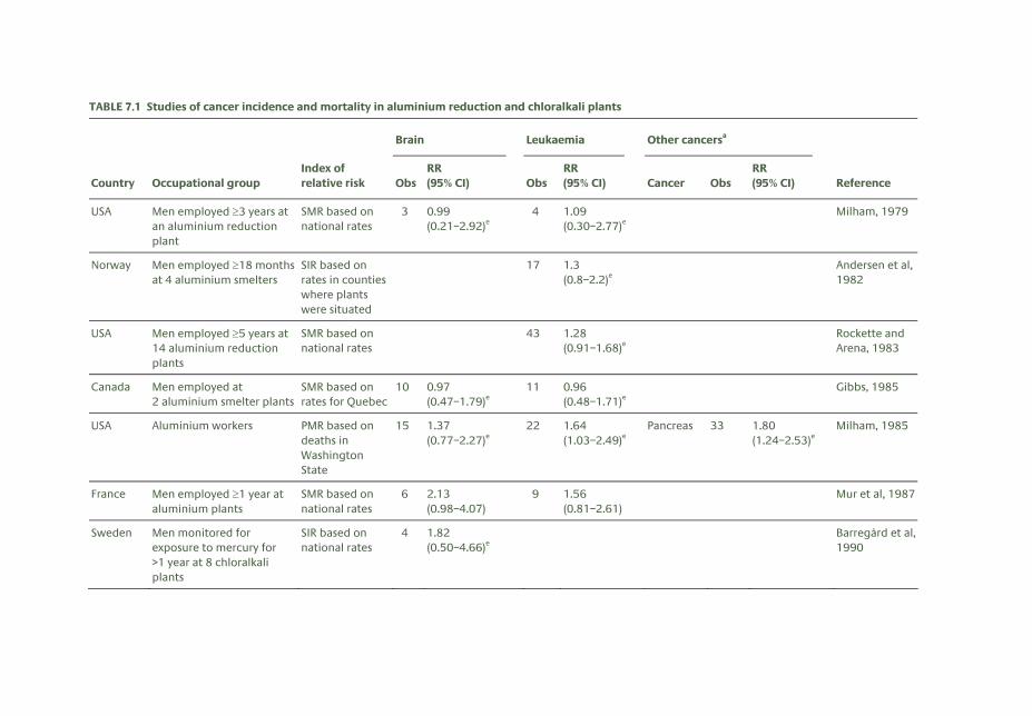
TABLE 7.1 Studies of cancer incidence and mortality in aluminium reduction and chloralkali plants
Brain Leukaemia Other cancersa
Country Occupational group Index of relative risk Obs
RR (95% CI) Obs
RR (95% CI) Cancer Obs
RR (95% CI) Reference
USA Men employed ≥3 years at an aluminium reduction plant
SMR based on national rates
3 0.99 (0.21–2.92)e
4 1.09 (0.30–2.77)e
Milham, 1979
Norway Men employed ≥18 months at 4 aluminium smelters
SIR based on rates in counties where plants were situated
17 1.3 (0.8–2.2)e
Andersen et al, 1982
USA Men employed ≥5 years at 14 aluminium reduction plants
SMR based on national rates
43 1.28 (0.91–1.68)e
Rockette and Arena, 1983
Canada Men employed at 2 aluminium smelter plants
SMR based on rates for Quebec
10 0.97 (0.47–1.79)e
11 0.96 (0.48–1.71)e
Gibbs, 1985
USA Aluminium workers PMR based on deaths in Washington State
15 1.37 (0.77–2.27)e
22 1.64 (1.03–2.49)e
Pancreas 33 1.80 (1.24–2.53)e
Milham, 1985
France Men employed ≥1 year at aluminium plants
SMR based on national rates
6 2.13 (0.98–4.07)
9 1.56 (0.81–2.61)
Mur et al, 1987
Sweden Men monitored for exposure to mercury for >1 year at 8 chloralkali plants
SIR based on national rates
4 1.82 (0.50–4.66)e
Barregård et al, 1990
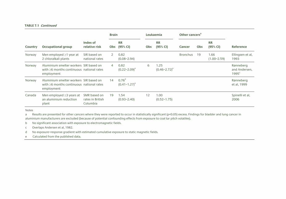
TABLE 7.1 Continued
Brain Leukaemia Other cancersa
Country Occupational group Index of relative risk Obs
RR (95% CI) Obs
RR (95% CI) Cancer Obs
RR (95% CI) Reference
Norway Men employed ≥1 year at 2 chloralkali plants
SIR based on national rates
2 0.82 (0.08–2.94)
Bronchus 19 1.66 (1.00–2.59)
Ellingsen et al, 1993
Norway Aluminium smelter workers with ≥6 months continuous employment
SIR based on national rates
4 0.82 (0.22–2.09)e
6 1.25 (0.46–2.72)e
Rønneberg and Andersen, 1995c
Norway Aluminium smelter workers with ≥6 months continuous employment
SIR based on national rates
14 0.76d (0.41–1.27)e
Rønneberg et al, 1999
Canada Men employed ≥3 years at an aluminium reduction plant
SMR based on rates in British Columbia
19 1.54 (0.93–2.40)
12 1.00 (0.52–1.75)
Spinelli et al, 2006
Notes a Results are presented for other cancers where they were reported to occur in statistically significant (p<0.05) excess. Findings for bladder and lung cancer in aluminium manufacturers are excluded (because of potential confounding effects from exposure to coal tar pitch volatiles).
b No significant association with exposure to electromagnetic fields.
c Overlaps Andersen et al, 1982.
d No exposure–response gradient with estimated cumulative exposure to static magnetic fields.
e Calculated from the published data.
7 H U M A N E X P O S U R E S : E P I D E M I O L O G I C A L S T U D I E S E T C
120
Overall, the strongest indication of elevated risk is for leukaemia, with higher than expected rates in six of the eight studies for which findings are reported. However, the numbers of observed cases in these studies are relatively small (see Table 7.1), and the highest relative risk reported was only 1.64. In view of this, and the potential for selective reporting of positive results, the findings do not point strongly to a risk of leukaemia from exposure to static magnetic fields, and at most can only be considered weak evidence for a cancer hazard. Nor is there any consistent evidence for an increased risk of brain tumours or of other types of cancer.
Bowman et al (1995) have hypothesised that the risk of childhood leukaemia might depend on exposure to specific combinations of static and extremely low frequency (ELF) magnetic fields. From laboratory data on calcium efflux from cells and diatom mobility, they predicted 19 bands of static magnetic field magnitudes, in conjunction with which exposure to 60 Hz fields would have an effect. They then looked for evidence of such interaction, using data from a case–control study of childhood leukaemia in Los Angeles County. Among 26 cases and 20 controls who were exposed to static magnetic fields in predicted bands of higher risk (centred at 38.0 and 50.6 μT), there was a statistically significant trend of increasing risk with higher exposure to ELF magnetic fields (fields were measured in the child’s bedroom at the home in southern California where he or she had lived longest).
This study had several weaknesses, which its authors acknowledged, including an inability to adjust for potential confounding factors and the limited scope of the measurements of magnetic fields. In addition, they noted the sensitivity of the findings to modification of the parameters specified in their hypothesis, and the absence of an established biophysical mechanism that would explain the proposed effect. For these reasons, the results can only be regarded as preliminary, and need confirmation by further research.
One of the mechanisms whereby hazardous agents can increase cancer risk is through cytogenetic damage to cells. It is unclear how such damage might arise from static or ELF magnetic field exposure. Nevertheless, one study has compared various cytogenetic parameters (sister chromatid exchanges, chromatid and chromosomal aberrations, and aneuploidy) in 13 engineers from a high voltage laboratory, who were exposed to static and alternating magnetic fields of 5–15 μT, and 13 unexposed production workers, matched for age and smoking habits (Skyberg et al, 1993). No statistically significant differences were observed overall, but in a subset of seven matched pairs who smoked, chromosome breaks were significantly more common in the exposed engineers. Given the small size and low statistical power of the study, the multiple effects examined, and the potential for concomitant exposure to time-varying fields, little can be concluded from it about the risk of cytogenetic abnormalities from static magnetic fields.
7.2 Reproductive and developmental outcomes
Several studies have examined reproductive and developmental outcomes in relation to exposures to static magnetic fields, either from MRI or from work in electrolytic industrial processes.
In 1990, a cross-sectional postal survey of reproductive health was carried out in women employed at more than 90% of the clinical MRI facilities in the USA (Evans et al, 1993; Kanal et al, 1993). The response

R E P R O D U C T I V E A N D D E V E L O P M E N T A L O U T C O M E S
121
rate was uncertain because the investigators could not enumerate the study population, but among 1915 responders, there had been 1421 pregnancies. Relative risks (RRs) for adverse outcomes were estimated for the 287 pregnancies that occurred while the respondents were working at an MRI unit as compared with 964 that occurred during work elsewhere. No statistically significant differences were found for delayed conception in planned pregnancies (RR 0.90, 95% CI 0.54–1.51), miscarriage (RR 1.27, 95% CI 0.92–1.77), delivery before 39 weeks (RR 1.19, 95% CI 0.76–1.88), birthweight under 2.5 kg (RR 1.01, 95% CI 0.50–2.04), or the sex ratio of babies.
In contrast to the reported normal sex ratio among babies born to female MRI workers, Milham (1993) found a statistically significant deficit of males (53 boys versus 86 girls) in children born in Washington State, USA, during 1980–90, whose fathers worked as carbon setters in aluminium reduction plants (a job with relatively high exposure to magnetic fields). Against this, in an analysis of all births in Norway during 1970–93, the proportion of males among children whose fathers worked in aluminium plants (50.38%) was not significantly different from that in those whose parents were unexposed to strong static or ELF magnetic fields (RR 0.98, 95% CI 0.94–1.03) (Irgens et al, 1997). The proportion of male offspring born to mothers working in aluminium plants (37.04%) was unusually low (RR 0.72, 95% CI 0.59–0.90), but this observation has not been confirmed in other studies.
In France, Mur et al (1998) compared birth rates after marriage in 692 potroom workers at an aluminium smelter and a control group of 588 workers from the same plant. The potroom workers were exposed to static magnetic fields up to 30 mT, but most of the time less than 20 mT. The study was restricted to men who had worked for at least one year at the plant, and who had married after starting this employment. The birth rate was significantly higher in the exposed group than in the control group, suggesting no adverse effect of the exposure on fertility.
A series of papers from the University of Nottingham has described outcomes in children who were examined in utero by echo-planar MRI. In the first report, when assessments were made at the age of three years in a sample of 20 children, no demonstrable disease or disability was found that could be attributed to the imaging (Baker et al, 1994).
In the second study, 74 women who volunteered for echo-planar MRI, using a 0.5 T static field for up to five serial scans, were compared with controls who underwent detailed second trimester ultrasound scans in the same time period (Myers et al, 1998). The controls were matched on a score for age, parity, ethnic origin, smoking history, and postcode. The babies born to the MRI group had significantly lower mean birthweights (3.33 versus 3.50 kg), which appeared to result from lower gestation at delivery (39.1 versus 39.8 weeks). This may have been because greater medical input led to a higher rate of induced deliveries. There was also one stillbirth and one neonatal death in the MRI group, but there were no statistically significant differences in APGAR scores at birth.
The third report describes a paediatric assessment at the age of nine months in 20 infants exposed to MRI in utero and 32 controls matched for mode of delivery, sex, gestation at delivery, and postcode (Clements et al, 2000). It is unclear exactly how subjects were selected, or whether all subjects eligible for study were recruited. Gross motor function was significantly advanced in the exposed children, but otherwise there was little difference between the two groups in their development or clinical history.
7 H U M A N E X P O S U R E S : E P I D E M I O L O G I C A L S T U D I E S E T C
122
In the Netherlands, Kok et al (2004) followed up 41 children whose mothers had been investigated by MRI (1.5 T) during the third trimester of pregnancy. Information about possible adverse health outcomes was obtained from birth records, through a questionnaire sent to the mothers, through a neurological examination three months after birth (in 33 of the children), and from routine health screening at infant healthcare centres up to three years of age. No abnormalities were observed in 37 of the 41 children. One child had impaired vision in one eye, and another impaired hearing following frequent ear infections, but the authors considered these unrelated to MRI exposure. A third child had impaired articulation, and a fourth was observed to have a rigid walking pattern and delayed speech at two years. This last child was born following growth restriction in utero, the onset of which preceded the MRI investigation.
7.3 Therapeutic trials using static magnetic fields
Another source of information on possible adverse effects of static magnetic fields is the literature on experimental studies in which magnetic devices have been tested for their ability to alleviate pain and associated symptoms. Such devices have been used for centuries to treat pain (Holcomb et al, 1991), and various possible mechanisms of action have been proposed. Anecdotally, there have been reports of benefit (Weintraub, 1998; Segal et al, 1999; Holcomb et al, 2000), but because of the strong potential for placebo effects, these reports carry little weight.
More rigorous evidence for or against effects is provided by blinded, randomised, experimental trials (Table 7.2). These studies have focused on various painful disorders, using a variety of magnetic devices applied over the affected anatomical areas or worn at the wrist for periods ranging from minutes to weeks. Fields at the surfaces of the magnets have been in the range 15–200 mT. In addition to changes in pain, some studies have assessed more objective indices of neurological function. Results relating to pain and other primary endpoints have been inconsistent, and the evidence for benefits is weak. However, there are no reports of material adverse effects.
7.4 Immune function
Data on leucocyte counts were obtained as part of a cross-sectional comparison of 320 workers exposed to static magnetic fields of up to 20 mT in three electrolysis plants in the USA and Canada and 186 unexposed controls (Marsh et al, 1982). Total leucocyte counts and the proportion of monocytes tended to be lower with higher exposures to horizontal magnetic fields, but there was no association with vertical magnetic fields.
Prompted by a cluster of five B-cell lymphomas at an aluminium reduction plant, Davis and Milham (1990) undertook a small pilot study to assess immune function in 23 apparently healthy workers from the same plant. Multiple indices of immune function were measured, including total lymphocyte count, c-reactive protein, beta-2 microglobulin and counts of cells according to cell surface antigens (T8, T11, IL2, MO2, TAC, T4, 4B4, 2H4, B4 and Leu1). Absolute T8 values were significantly higher for the 15 potroom workers than for non-potroom workers, and were also markedly higher than normal population values.
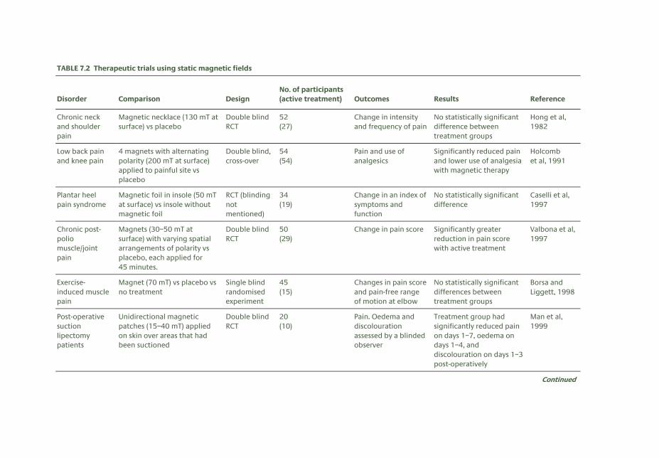
TABLE 7.2 Therapeutic trials using static magnetic fields
Disorder Comparison Design No. of participants (active treatment) Outcomes Results Reference
Chronic neck and shoulder pain
Magnetic necklace (130 mT at surface) vs placebo
Double blind RCT
52 (27)
Change in intensity and frequency of pain
No statistically significant difference between treatment groups
Hong et al, 1982
Low back pain and knee pain
4 magnets with alternating polarity (200 mT at surface) applied to painful site vs placebo
Double blind, cross-over
54 (54)
Pain and use of analgesics
Significantly reduced pain and lower use of analgesia with magnetic therapy
Holcomb et al, 1991
Plantar heel pain syndrome
Magnetic foil in insole (50 mT at surface) vs insole without magnetic foil
RCT (blinding not mentioned)
34 (19)
Change in an index of symptoms and function
No statistically significant difference
Caselli et al, 1997
Chronic post-polio muscle/joint pain
Magnets (30–50 mT at surface) with varying spatial arrangements of polarity vs placebo, each applied for 45 minutes.
Double blind RCT
50 (29)
Change in pain score Significantly greater reduction in pain score with active treatment
Valbona et al, 1997
Exercise-induced muscle pain
Magnet (70 mT) vs placebo vs no treatment
Single blind randomised experiment
45 (15)
Changes in pain score and pain-free range of motion at elbow
No statistically significant differences between treatment groups
Borsa and Liggett, 1998
Post-operative suction lipectomy patients
Unidirectional magnetic patches (15–40 mT) applied on skin over areas that had been suctioned
Double blind RCT
20 (10)
Pain. Oedema and discolouration assessed by a blinded observer
Treatment group had significantly reduced pain on days 1–7, oedema on days 1–4, and discolouration on days 1–3 post-operatively
Man et al, 1999
Continued
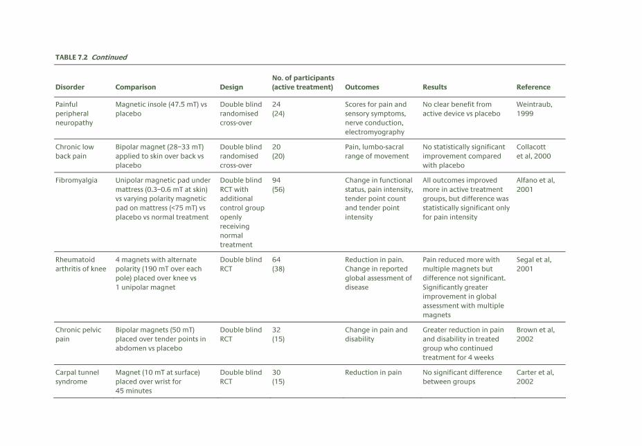
TABLE 7.2 Continued
Disorder Comparison Design No. of participants (active treatment) Outcomes Results Reference
Painful peripheral neuropathy
Magnetic insole (47.5 mT) vs placebo
Double blind randomised cross-over
24 (24)
Scores for pain and sensory symptoms, nerve conduction, electromyography
No clear benefit from active device vs placebo
Weintraub, 1999
Chronic low back pain
Bipolar magnet (28–33 mT) applied to skin over back vs placebo
Double blind randomised cross-over
20 (20)
Pain, lumbo-sacral range of movement
No statistically significant improvement compared with placebo
Collacott et al, 2000
Fibromyalgia Unipolar magnetic pad under mattress (0.3–0.6 mT at skin) vs varying polarity magnetic pad on mattress (<75 mT) vs placebo vs normal treatment
Double blind RCT with additional control group openly receiving normal treatment
94 (56)
Change in functional status, pain intensity, tender point count and tender point intensity
All outcomes improved more in active treatment groups, but difference was statistically significant only for pain intensity
Alfano et al, 2001
Rheumatoid arthritis of knee
4 magnets with alternate polarity (190 mT over each pole) placed over knee vs 1 unipolar magnet
Double blind RCT
64 (38)
Reduction in pain. Change in reported global assessment of disease
Pain reduced more with multiple magnets but difference not significant. Significantly greater improvement in global assessment with multiple magnets
Segal et al, 2001
Chronic pelvic pain
Bipolar magnets (50 mT) placed over tender points in abdomen vs placebo
Double blind RCT
32 (15)
Change in pain and disability
Greater reduction in pain and disability in treated group who continued treatment for 4 weeks
Brown et al, 2002
Carpal tunnel syndrome
Magnet (10 mT at surface) placed over wrist for 45 minutes
Double blind RCT
30 (15)
Reduction in pain No significant difference between groups
Carter et al, 2002
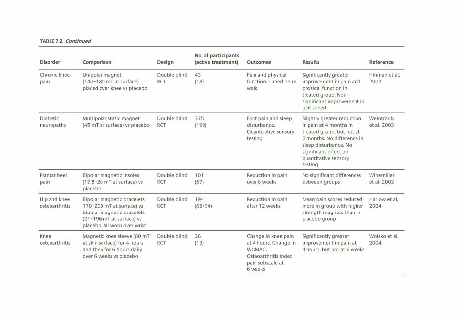
TABLE 7.2 Continued
Disorder Comparison Design No. of participants (active treatment) Outcomes Results Reference
Chronic knee pain
Unipolar magnet (140–180 mT at surface) placed over knee vs placebo
Double blind RCT
43 (18)
Pain and physical function. Timed 15 m walk
Significantly greater improvement in pain and physical function in treated group. Non-significant improvement in gait speed
Hinman et al, 2002
Diabetic neuropathy
Multipolar static magnet (45 mT at surface) vs placebo
Double blind RCT
375 (199)
Foot pain and sleep disturbance. Quantitative sensory testing
Slightly greater reduction in pain at 4 months in treated group, but not at 2 months. No difference in sleep disturbance. No significant effect on quantitative sensory testing
Weintraub et al, 2003
Plantar heel pain
Bipolar magnetic insoles (17.8–20 mT at surface) vs placebo
Double blind RCT
101 (57)
Reduction in pain over 8 weeks
No significant differences between groups
Winemiller et al, 2003
Hip and knee osteoarthritis
Bipolar magnetic bracelets 170–200 mT at surface) vs bipolar magnetic bracelets (21–196 mT at surface) vs placebo, all worn over wrist
Double blind RCT
194 (65+64)
Reduction in pain after 12 weeks
Mean pain scores reduced more in group with higher strength magnets than in placebo group
Harlow et al, 2004
Knee osteoarthritis
Magnetic knee sleeve (80 mT at skin surface) for 4 hours and then for 6 hours daily over 6 weeks vs placebo
Double blind RCT
26 (13)
Change in knee pain at 4 hours. Change in WOMAC. Osteoarthritis index pain subscale at 6 weeks
Significantly greater improvement in pain at 4 hours, but not at 6 weeks
Wolsko et al, 2004
7 H U M A N E X P O S U R E S : E P I D E M I O L O G I C A L S T U D I E S E T C
126
T4/T8 ratios also tended to be abnormal in potroom workers. No follow-up of the pilot investigation appears to have been reported, and, in the absence of independent replication with larger numbers of subjects and closer attention to potential confounding effects, no strong conclusions can be drawn.
In another cross-sectional survey, Tuschl et al (2000) assessed indices of immune function in 10 workers exposed to time-varying magnetic fields from induction heaters, 10 medical assistants carrying out MRI scans, and 23 unexposed controls. The outcomes studied included relative and absolute numbers of lymphocyte subsets; proliferative activity of T- and B-cells; production of interleukin 2, interferon gamma and tumour necrosis factor alpha; and the oxidative bursts of monocytes and granulocytes. The numbers of natural killer cells were significantly elevated in workers exposed to fields from induction heaters, and their monocyte oxidative burst was significantly reduced, but none of the measures in MRI workers was significantly different from those in controls. Again, because of the small size of the study, no firm conclusions can be drawn.
More recently, Salvatore et al (2003) reported a Phase 1 clinical trial to assess the safety and toxicity of the combination of a static magnetic field (28 mT at 1 cm from the source, which was placed over the liver) in 12 patients with advanced malignancy. No increase in toxicity to white blood cell count and platelet count was seen in comparison with 12 historical control subjects who received only chemotherapy.
7.5 Other health outcomes
The relation of static magnetic fields to musculoskeletal disorders was explored in two studies at a Norwegian aluminium reduction plant. In the first investigation, the prevalence of musculoskeletal symptoms was compared in workers employed in the potrooms, who were exposed to static magnetic fields of 20–30 mT, and a control group of workers from the same factory, who had only background levels of exposure (Moen et al, 1995). After adjustment for age, rates of symptoms were similar in the two groups, although the power to detect even a moderate effect was low (the upper 95% confidence limits for odds ratios all exceeded three). A further limitation was that the assessment of symptoms was based on information obtained at routine medical examinations, and was not fully standardised. Also, it is possible that some symptomatic workers had transferred from the potrooms to other, less demanding work.
The second investigation compared rates of sick leave for musculoskeletal disorders over a five-year period in 342 workers exposed to average fields of 8 mT and 222 unexposed controls (Moen et al, 1996). There was no difference between the two groups, either in the frequency of periods of absence for musculoskeletal problems or in the duration of such absence.
As described in Chapter 6, a cross-sectional survey in the Netherlands compared acute symptoms and cognitive performance in 18 workers in an MRI equipment manufacturing department and 20 unexposed controls in another department of the same factory (de Vocht et al, 2006). The estimated average exposures of the MRI-exposed group were 25.9 mT over 8 hours for a 1.0 T system and 40.4 mT over 8 hours for a 1.5 T system. Vertigo, metallic taste and difficulties with concentration were all significantly (p<0.05) more common in the exposed workers and, along with tinnitus, were particularly
R E F E R E N C E S
127
frequent in the most highly exposed group who worked near to a 1.5 T system. Among the MRI-exposed group, most of the complaints were more common in those who were observed to move more rapidly while working in the RF cage near to the magnets.
7.6 Summary and conclusions
Overall, the balance of evidence from epidemiological studies, randomised trials and clinical case reports does not clearly indicate any long-term adverse health effects from exposure to static magnetic fields. However, many of the published studies lack statistical power or suffer from other methodological weaknesses, and this limits the reassurance of safety that they provide. The most extensive evidence relates to risks of cancer in workers employed at electrolysis plants. In these occupations, there is slight but not persuasive evidence of a small increase in the risk of leukaemia. Of particular note is the absence of any published epidemiological studies on mortality or cancer incidence in patients investigated by MRI, or in healthcare workers and scientific researchers who carry out MRI investigations. There is limited epidemiological evidence, based on a single study, that complaints such as vertigo and metallic taste are more common in people working near to MRI magnets.
7.7 References Alfano AP, Taylor AG, Foresman PA, Dunkl PR, McConnell GG, Conaway MR and Gillies GT (2001). Static magnetic
fields for treatment of fibromyalgia: a randomized controlled trial. J Altern Complement Med, 7, 53–64.
Andersen A, Dahlberg BE, Magnus K and Wannag A (1982). Risk of cancer in the Norwegian aluminium industry. Int J Cancer, 29, 295–8.
Baker PN, Johnson IR, Harvey PR, Gowland PA and Mansfield P (1994). A three-year follow-up of children imaged in utero with echo-planar magnetic resonance. Am J Obstet Gynecol, 170, 32–3.
Barregård L, Järvholm B and Ungethüm E (1985). Cancer among workers exposed to strong static magnetic fields. Lancet, 2, 892.
Barregård L, Sällsten G and Järvholm B (1990). Mortality and cancer incidence in chloralkali workers exposed to inorganic mercury. Br J Ind Med, 47, 99–104.
Borsa PA and Liggett CL (1998). Flexible magnets are not effective in decreasing pain perception and recovery time after muscle microinjury. J Athlet Train, 33, 150–55.
Bowman JD, Thomas DC, London SJ and Peters JM (1995). Hypothesis: the risk of childhood leukemia is related to combinations of power-frequency and static magnetic fields. Bioelectromagnetics, 16, 48–59.
Brown CS, Ling FW, Wan JY and Pilla AA (2002). Efficacy of static magnetic field therapy in chronic pelvic pain: a double-blind pilot study. Am J Obstet Gynecol, 187, 1581–7.
Carter R, Aspy CB and Mold J (2002). The effectiveness of magnet therapy for treatment of wrist pain attributed to carpal tunnel syndrome. J Fam Pract, 51, 38–40.
Caselli MA, Clark N, Lazarus S, Velez Z and Venegas L (1997). Evaluation of magnetic foil and PPT insoles in the treatment of heel pain. J Am Podiatr Med Assoc, 87, 11–16.
Clements H, Duncan KR, Fielding K, Gowland PA, Johnson IR and Baker PN (2000). Infants exposed to MRI in utero have a normal paediatric assessment at 9 months of age. Br J Radiol, 73, 190–94.
Collacott EA, Zimmerman JT, White DW and Rindone JP (2000). Bipolar permanent magnets for the treatment of chronic low back pain: a pilot study. JAMA, 283, 1322–5.
Davis RL and Milham S (1990). Altered immune status in aluminum reduction plant workers. Am J Ind Med, 18, 79–85.
7 H U M A N E X P O S U R E S : E P I D E M I O L O G I C A L S T U D I E S E T C
128
de Vocht F, van Drooge H, Engels H and Kromhout H (2006). Exposure, health complaints and cognitive performance among employees of an MRI scanners manufacturing department. J Magn Reson Imaging, 23, 197–204.
Ellingsen DG, Andersen A, Nordhagen HP, Efskind J and Kjuus H (1993). Incidence of cancer and mortality among workers exposed to mercury vapour in the Norwegian chloralkali industry. Br J Ind Med, 50, 875–80.
Evans JA, Savitz DA, Kanal E and Gillen J (1993). Infertility and pregnancy outcome among magnetic resonance imaging workers. J Occup Med, 35, 1191–5.
Gibbs GW (1985). Mortality of aluminum reduction plant workers, 1950 through 1977. J Occup Med, 27, 761–70.
Harlow T, Greaves C, White A, Brown L, Hart A and Ernst E (2004). Randomised controlled trial of magnetic bracelets for relieving pain in osteoarthritis of the hip and knee. Br Med J, 329, 1450–54.
Hinman MR, Ford J and Heyl H (2002). Effects of static magnets on chronic knee pain and physical function: a double-blind study. Altern Ther Health Med, 8, 50–55.
Holcomb RR, Parker RA and Harrison MS (1991). Isomagnetics in the treatment of human pain: past, present, future. Environ Med, 8, 24–30.
Holcomb RR, Worthington WB, McCullough BA and McLean MJ (2000). Static magnetic field therapy for pain in the abdomen and genitals. Pediatr Neurol, 23, 261–4.
Hong CZ, Lin JC, Bender LF, Schaeffer JN, Meltzer RJ and Causin P (1982). Magnetic necklace: its therapeutic effectiveness on neck and shoulder pain. Arch Phys Med Rehabil, 63, 462–6.
Irgens Å, Krüger K, Skorve AH and Irgens LM (1997). Male proportion in offspring of parents exposed to strong static and extremely low-frequency electromagnetic fields in Norway. Am J Ind Med, 32, 557–61.
Kanal E, Gillen J, Evans JA, Savitz DA and Shellock FG (1993). Survey of reproductive health among female MR workers. Radiology, 187, 395–9.
Kok RD, de Vries MM, Heerschap A and van den Berg PP (2004). Absence of harmful effects of magnetic resonance exposure at 1.5 T in utero during the third trimester of pregnancy: a follow-up study. Magn Reson Imaging, 22, 851–4.
Man D, Man B and Plosker H (1999). The influence of permanent magnetic field therapy on wound healing in suction lipectomy patients: a double-blind study. Plast Reconstr Surg, 104, 2261–6.
Marsh JL, Armstrong TJ, Jacobson AP and Smith RG (1982). Health effect of occupational exposure to steady magnetic fields. Am Ind Hyg Assoc J, 43, 387–94.
Milham S (1979). Mortality in aluminum reduction plant workers. J Occup Med, 21, 475–80.
Milham S (1985). Mortality in workers exposed to electromagnetic fields. Environ Health Perspect, 62, 297–300.
Milham S (1993). Unusual sex ratio of births to carbon setter fathers. Am J Ind Med, 23, 829–31.
Moen BE, Drabløs PA, Pedersen S, Sjøen M and Thommesen G (1995). Symptoms of the musculoskeletal system and exposure to magnetic fields in an aluminium plant. Occup Environ Med, 52, 524–7.
Moen BE, Drabløs PA, Pedersen S, Sjøen M and Thommesen G (1996). Absence of relation between sick leave caused by musculoskeletal disorders and exposure to magnetic fields in an aluminium plant. Bioelectromagnetics, 17, 37–43.
Mur JM, Moulin JJ, Meyer-Bisch C, Massin N, Coulon JP and Loulergue J (1987). Mortality of aluminium reduction plant workers in France. Int J Epidemiol, 16, 257–64.
Mur JM, Wild P, Rapp R, Vautrin JP and Coulon JP (1998). Demographic evaluation of the fertility of aluminium industry workers: influence of exposure to heat and static magnetic fields. Hum Reprod, 13, 2016–19.
Myers C, Duncan KR, Gowland PA, et al (1998). Failure to detect intrauterine growth restriction following in utero exposure to MRI. Br J Radiol, 71, 549–51.
Rockette HE and Arena VC (1983). Mortality studies of aluminium reduction plant workers: potroom and carbon department. J Occup Med, 25, 549–57.
Rønneberg A (1995). Mortality and cancer morbidity in workers from an aluminium smelter with prebaked carbon anodes – Part 1: exposure assessment. Occup Environ Med, 52, 242–9.
Rønneberg A and Andersen A (1995). Mortality and cancer morbidity in workers from an aluminium smelter with prebaked carbon anodes – Part II: cancer morbidity. Occup Environ Med, 52, 250–54.
R E F E R E N C E S
129
Rønneberg A, Haldorsen T, Romundstad P and Andersen A (1999). Occupational exposure and cancer incidence among workers from an aluminium smelter in western Norway. Scand J Work Environ Health, 25, 207–14.
Salvatore JR, Harrington J and Kummet T (2003). Phase 1 clinical study of a static magnetic field combined with anti-neoplastic chemotherapy in the treatment of human malignancy: initial safety and toxicity data. Bioelectromagnetics, 24, 524–27.
Segal NA, Huston J, Fuchs H, Holcomb R and McLean MJ (1999). Efficacy of a static magnetic device against knee pain associated with inflammatory arthritis. J Clin Rheumatol, 5, 302–5.
Segal NA, Toda Y, Huston J, Saeki Y, Shimizu M, Fuchs H, Shimaoka Y, Holcomb R and McLean MJ (2001). Two configurations of static magnetic fields for treating rheumatoid arthritis of the knee: a double-blind clinical trial. Arch Phys Med Rehabil, 82, 1453–60.
Skyberg K, Hansteen IL and Vistnes AI (1993). Chromosome aberrations in lymphocytes of high-voltage laboratory cable splicers exposed to electromagnetic fields. Scand J Work Environ Health, 19, 29–34.
Spinelli JJ, Demers PA, Le ND, Friesen MD, Lorenzi MF, Fang R and Gallagher RP (2006). Cancer risk in aluminium reduction plant workers (Canada). Cancer Causes Control, 17, 939–48.
Tuschl H, Neubauer G, Schmid G, Weber E and Winker N (2000). Occupational exposure to static, ELF, VF and VLF magnetic fields and immune parameters. Int J Occup Med Environ Health, 13, 39–50.
Vallbona C, Hazlewood CF and Jurida G (1997). Response of pain to static magnetic fields in postpolio patients: a double-blind pilot study. Arch Phys Med Rehabil, 78, 1200–1203.
Weintraub MI (1998). Chronic submaximal magnetic stimulation in peripheral neuropathy: Is there a beneficial therapeutic relationship? Am J Pain Manage, 8, 12–16.
Weintraub MI (1999). Magnetic bio-stimulation in painful diabetic peripheral neuropathy: a novel intervention – a randomized, double-placebo crossover study. Am J Pain Manage, 9, 8–17.
Weintraub MI, Wolfe GI, Barohn RA, Cole SP, Parry GJ, Hayat G, Cohen JA, Page JC, Bromberg MB and Schwartz SL; Magnetic Research Group (2003). Static magnetic field therapy for symptomatic diabetic neuropathy: a randomized, double-blind, placebo-controlled trial. Arch Phys Med Rehabil, 84, 736–46.
Winemiller MH, Billow RG, Laskowski ER and Harmsen WS (2003). Effect of magnetic vs sham-magnetic insoles on plantar heel pain: a randomised controlled trial. JAMA, 290, 1474–8.
Wolsko PM, Eisenberg DM, Simon LS, Davis RB, Walleczek J, Mayo-Smith M, Kaptchuk TJ and Phillips RS (2004). Double-blind placebo-controlled trial of static magnets for the treatment of osteoarthritis of the knee: results of a pilot study. Altern Ther Health Med, 10, 36–43.
130
8 Conclusions
8.1 Sources, exposures and measurements
Exposure to the geomagnetic field, which varies from 25 to 60 μT over inhabited parts of the world’s surface, is ubiquitous. This field is readily perturbed by ferromagnetic materials in buildings, transport systems and other man-made structures, giving rise to local variations in its strength over distances that are small in comparison to human body size. When multiple spot measurements were made inside individual rooms within people’s homes, typical standard deviations within the data were in the range 1–3 μT. Much greater perturbations were found near machinery in industrial premises and near transport systems, which had a large amount of steel in their fabric. In such situations, spot measurements were found to vary between a few microtesla and 120 μT, ie up to around twice the geomagnetic field.
Magnetic resonance imaging (MRI) scanners produce the strongest magnetic fields that people encounter over large parts of their body. MRI actually exposes staff to a number of different types of magnetic fields, including the static field, which is always present even when the scanner is not operating, and also time-varying fields. The time-varying fields fall into two classes: magnetic field gradients used for spatial encoding, which are switched at audio frequencies, and the radiofrequency (RF) fields used to excite the magnetic resonance signal. The switched gradient and RF fields are only present when scans are being performed, whereas the static fields are always present. Patients and volunteers can be exposed to fields up to a few tesla during scans, but staff are also exposed to the stray static field which extends around the scanner. Little information is available regarding levels of exposure for those whose work brings them close to the magnets.
Exposure of people to large magnetic fields from MRI is likely to increase in the next few decades, as MRI technology continues to develop, the range of applications broadens, and the examination costs decrease, particularly because of its ability to replace ionising radiation exposure. In particular, the field levels of the scanners are increasing to achieve better image quality. Furthermore open access scanners are being introduced, in particular to allow MR-guided interventional procedures, which are likely to increase staff exposure to the static field.
There are few other man-made sources and situations that can give rise to static magnetic field exposure at levels appreciably above the geomagnetic field. There have been several systematic investigations of exposures in industrial electrolysis facilities and these indicate exposures of staff working near the cells and conductors of a few millitesla throughout their working day, with exposures up to around 20 mT being possible in some places.
Some arc welding and resistance welding sources use DC supplies and so give rise to static magnetic fields in their vicinity. Operators of arc welding equipment, which uses currents up to around 600 A, often drape the cable over their shoulder and fields of a few millitesla have been measured at 1 cm from
M E C H A N I S M S F O R B I O L O G I C A L I N T E R A C T I O N
131
the cable. Resistance welding uses higher currents, up to 10 kA or more, and it seems that exposure up to millitesla levels is also possible, although there are few reported data.
Some transport systems, such as certain types of trains, contain DC motors and so have sources of static fields on-board. What measurements are available suggest that the fields at most locations are essentially similar to typical perturbed geomagnetic fields. However, air-cored smoothing inductors beneath the floors of some trains have been found to produce fields over 10 mT immediately above them at floor level.
The above source categories (welding, electrolysis and transport systems not powered by batteries) use DC supplies derived from rectification of AC supplies with or without some degree of smoothing of the current waveform applied. As a consequence, extremely low frequency (ELF) AC fields with frequency components that are harmonics of the AC signal are produced along with the static magnetic fields. There are very few situations where static fields are produced without AC fields present and these would include applications such as MRI, high voltage DC power lines and a range of scientific applications using electromagnets to deflect particle and plasma beams.
For practical exposure assessment purposes static magnetic fields are usually measured with a fluxgate magnetometer or a Hall effect sensor, and instruments available are based on either of these technologies. Fluxgate magnetometers are the more sensitive, typically covering 0.1 nT to 10 mT, and Hall effect probes typically cover 10 μT to 100 T.
8.2 Mechanisms for biological interaction
Calculations of the magnitude of magnetohydrodynamic forces in blood vessels suggest they are too small to produce appreciable biological effects at field levels presently used in MRI. They show that the changes in the flow of blood in the aorta vary as B 2 and are around 5% for a 10 T field. These changes are for field components perpendicular to blood vessels and no change should occur for parallel components. Now while the axial field within an MRI magnet is largely parallel to most of the aorta, it is approximately perpendicular to the aortic arch. Fields normal to the aorta are also experienced by people standing near the mouth of the MRI magnet and could be experienced near to other high field magnets but, in these situations, the fields would usually be very much less than 10 T so that the flow changes would be very small. Analysis of the effects of magnetohydrodynamic forces on the vestibular system suggest they are too small to produce vertigo, although this conclusion is still somewhat controversial.
Estimates of the size of the induced currents caused by head and body movement in regions where the field gradient is large, such as those occurring near a 7 T MRI magnet, appear to be somewhat lower than the threshold values at which peripheral nerve stimulation can be sensed. It is not clear, however, what margin of safety exists without further characterisation of the currents induced by body movement in such fields.
It would seem likely that the vertigo experienced by a number of people inside and near to MRI magnets involves interactions within the vestibular system of the inner ear. Experiments suggest that two very different interactions may be involved. One is the result of the currents induced by head movements in a field and calculations suggest that these are large enough to alter the firing rate of the afferent nerves on
8 C O N C L U S I O N S
132
to which the hair cells synapse (galvanic vestibular stimulation). Another interaction, the magneto-Archimedes effect, occurs when people are stationary in a field gradient. The gradient leads to a force on the otolith proportional to the product of the field and the field gradient (B dB/dz), which arises from the fact that its diamagnetic susceptibility differs from that of the surrounding endolymphatic fluid. Calculations show that, in a 7 T MRI magnet, the resulting accelerations can be up to ten times the threshold value so that it seems likely that effects caused by this mechanism might also be apparent in smaller magnets. Experiments do not provide clear-cut answers as to which mechanism is the more important. If vertigo were the result of the electric fields induced by body motion it would seem that the threshold for this is lower than that for peripheral nerve stimulation.
There have been a number of discussions of the metallic taste and of the magnetophosphenes experienced by some people in magnetic fields. Both seem likely to be the result of induced currents caused by head or body movement. The former is believed to be due to the release of metallic ions by electrolysis of saliva and the latter to involve direct electrical stimulation of the retina. Both effects disappear soon after the body stops moving.
The magnetite nanoparticles of radius around 100 nm or less that are present in some human tissue will be slightly displaced by a non-uniform magnetic field and, if they are attached to a cell membrane or cytoskeleton, the displacement might activate adjacent mechanosensitive ion channels. However, it would seem that the nanoparticles are too small for this to occur in or around magnets that are presently used even when the nanoparticles are strongly coupled with their neighbours in a cluster. This may not be the case, however, in people whose bodies contain micrometre-sized particles of iron as a result of being exposed to an atmosphere containing iron as a pollutant – for example, miners of iron ores or welders.
It is known that magnetic fields can produce appreciable changes in the rates of certain chemical reactions. There has been considerable effort made to see whether these include any biochemical reactions. So far though only one example has been found and this involved a protein found in plants but not in mammals.
8.3 Cellular studies
Cellular studies are used to assess potential effects in a well-defined and controlled way that would be difficult to achieve with in vivo studies. The studies cover a wide range in terms of both biological systems and magnetic flux densities. For weaker magnetic fields of less than 0.2 T the reproducibility of findings is poor and there is no apparent consistent or cohesive pattern in terms of exposure parameters or biological response; these studies have not been reviewed in this report. The effects of stronger magnetic fields (0.2–16.7 T) have also been tested in a wide variety of biological systems with durations ranging from minutes to months. Although macromolecules and cells can be shown to orientate in magnetic fields, other effects on cells are not so well established. There is evidence that cellular function may be affected through changes in gene expression or cellular signalling; however, this effect may be via the action on the growth conditions needed to maintain cells in the laboratory rather than a direct effect on the cells. Overall the evidence does not support a direct genotoxic effect but there are indications that exposure to strong magnetic fields may compromise the cellular defence mechanisms, making some cells less able to withstand other potentially harmful agents.
H U M A N E X P O S U R E S
133
8.4 Animal studies
There have been no systematic investigations of the biological effects of either acute or long-term exposure to static magnetic fields in animals, and the available data are incomplete and fragmentary. This is particularly true regarding the effects of intense fields of more than a few tesla.
The evidence concerning the carcinogenicity of static magnetic fields is inconclusive, and too few studies have been carried out to draw any firm conclusions. No long-term animal studies have investigated this possibility using intense fields, and the available evidence is limited to using relatively weak fields.
With regard to effects on fertility, growth and development, no consistent adverse effects have been demonstrated, but there have been few good studies, especially using fields in excess of 1 T. The existing evidence is uninformative regarding the effects that might ensue from exposure above this value.
There are a number of reports of field-related effects on the cardiovascular system, most notably on arterial blood pressure and skin blood flow, often at fields much less than 1 T, which have not been independently corroborated. In addition, electric potentials generated across the aorta and other major arteries by the flow of blood in a static magnetic field can be routinely seen in the electrocardiogram (ECG) of animals, including primates, exposed to fields in excess of 100 mT. However, it is unclear whether there are any meaningful physiological consequences. The potential for strong fields to cause effects has not been explored in detail.
Studies investigating the effects of static magnetic fields on the nervous system have tended to use weak fields (of less than 1 T) and have produced variable, and sometimes conflicting, results. However, the possibility remains that exposure may influence electrophysiological response. A series of papers, mainly from one laboratory, indicates that exposure to static magnetic fields above a threshold of 4–7 T may induce behavioural and neural changes in animals. Animals exposed to these fields may experience an unpleasant vestibular disturbance consistent with self-reports by people after similar exposures.
8.5 Human exposures
8.5.1 Cardiovascular effects
Static magnetic fields may theoretically affect the cardiovascular system by directly or indirectly influencing cellular function, cardiac rhythm, cardiac pump performance, vascular resistance and tissue perfusion.
Human studies of these effects are limited in their extent and methodology, particularly in the use of sham exposures and effective ‘blinding’ of both subjects and researchers. No detailed studies have been performed to identify the underlying mechanisms of the observed changes. No specific studies have been performed on subjects likely to be more vulnerable to the cardiovascular effects of exposure to static magnetic fields.
Although local currents arising from induced voltage related to the ascending aorta blood flow have been identified as a potential influence on cardiac pacemaker function or myocardial contractility, no studies have directly measured such local currents or confidently identified a related effect in vivo.
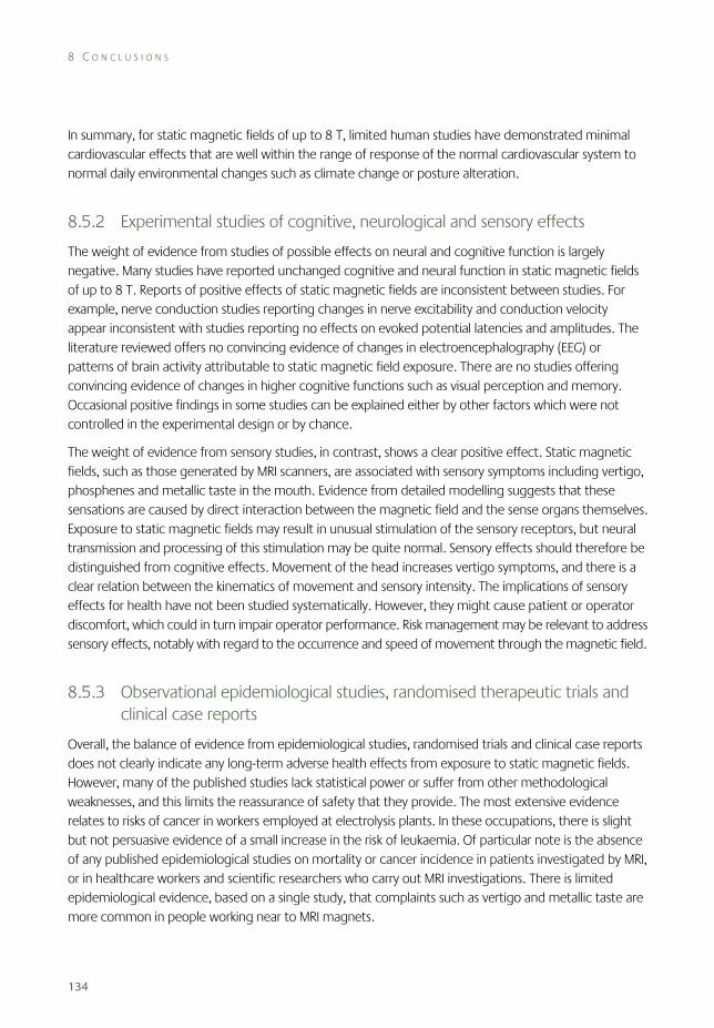
8 C O N C L U S I O N S
134
In summary, for static magnetic fields of up to 8 T, limited human studies have demonstrated minimal cardiovascular effects that are well within the range of response of the normal cardiovascular system to normal daily environmental changes such as climate change or posture alteration.
8.5.2 Experimental studies of cognitive, neurological and sensory effects
The weight of evidence from studies of possible effects on neural and cognitive function is largely negative. Many studies have reported unchanged cognitive and neural function in static magnetic fields of up to 8 T. Reports of positive effects of static magnetic fields are inconsistent between studies. For example, nerve conduction studies reporting changes in nerve excitability and conduction velocity appear inconsistent with studies reporting no effects on evoked potential latencies and amplitudes. The literature reviewed offers no convincing evidence of changes in electroencephalography (EEG) or patterns of brain activity attributable to static magnetic field exposure. There are no studies offering convincing evidence of changes in higher cognitive functions such as visual perception and memory. Occasional positive findings in some studies can be explained either by other factors which were not controlled in the experimental design or by chance.
The weight of evidence from sensory studies, in contrast, shows a clear positive effect. Static magnetic fields, such as those generated by MRI scanners, are associated with sensory symptoms including vertigo, phosphenes and metallic taste in the mouth. Evidence from detailed modelling suggests that these sensations are caused by direct interaction between the magnetic field and the sense organs themselves. Exposure to static magnetic fields may result in unusual stimulation of the sensory receptors, but neural transmission and processing of this stimulation may be quite normal. Sensory effects should therefore be distinguished from cognitive effects. Movement of the head increases vertigo symptoms, and there is a clear relation between the kinematics of movement and sensory intensity. The implications of sensory effects for health have not been studied systematically. However, they might cause patient or operator discomfort, which could in turn impair operator performance. Risk management may be relevant to address sensory effects, notably with regard to the occurrence and speed of movement through the magnetic field.
8.5.3 Observational epidemiological studies, randomised therapeutic trials and clinical case reports
Overall, the balance of evidence from epidemiological studies, randomised trials and clinical case reports does not clearly indicate any long-term adverse health effects from exposure to static magnetic fields. However, many of the published studies lack statistical power or suffer from other methodological weaknesses, and this limits the reassurance of safety that they provide. The most extensive evidence relates to risks of cancer in workers employed at electrolysis plants. In these occupations, there is slight but not persuasive evidence of a small increase in the risk of leukaemia. Of particular note is the absence of any published epidemiological studies on mortality or cancer incidence in patients investigated by MRI, or in healthcare workers and scientific researchers who carry out MRI investigations. There is limited epidemiological evidence, based on a single study, that complaints such as vertigo and metallic taste are more common in people working near to MRI magnets.
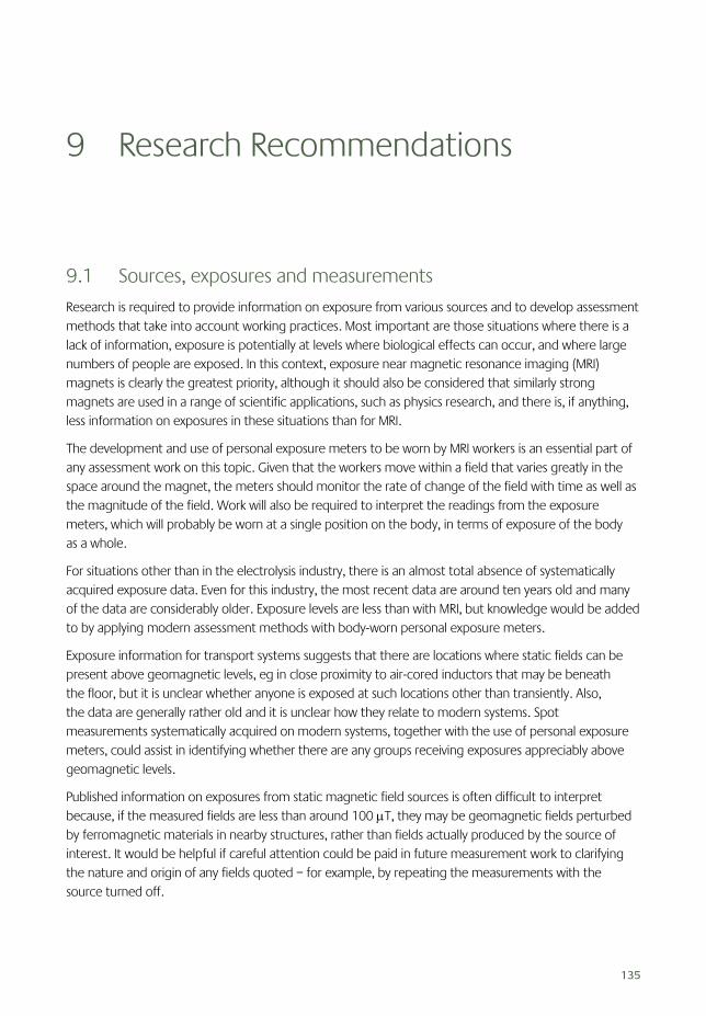
135
9 Research Recommendations
9.1 Sources, exposures and measurements
Research is required to provide information on exposure from various sources and to develop assessment methods that take into account working practices. Most important are those situations where there is a lack of information, exposure is potentially at levels where biological effects can occur, and where large numbers of people are exposed. In this context, exposure near magnetic resonance imaging (MRI) magnets is clearly the greatest priority, although it should also be considered that similarly strong magnets are used in a range of scientific applications, such as physics research, and there is, if anything, less information on exposures in these situations than for MRI.
The development and use of personal exposure meters to be worn by MRI workers is an essential part of any assessment work on this topic. Given that the workers move within a field that varies greatly in the space around the magnet, the meters should monitor the rate of change of the field with time as well as the magnitude of the field. Work will also be required to interpret the readings from the exposure meters, which will probably be worn at a single position on the body, in terms of exposure of the body as a whole.
For situations other than in the electrolysis industry, there is an almost total absence of systematically acquired exposure data. Even for this industry, the most recent data are around ten years old and many of the data are considerably older. Exposure levels are less than with MRI, but knowledge would be added to by applying modern assessment methods with body-worn personal exposure meters.
Exposure information for transport systems suggests that there are locations where static fields can be present above geomagnetic levels, eg in close proximity to air-cored inductors that may be beneath the floor, but it is unclear whether anyone is exposed at such locations other than transiently. Also, the data are generally rather old and it is unclear how they relate to modern systems. Spot measurements systematically acquired on modern systems, together with the use of personal exposure meters, could assist in identifying whether there are any groups receiving exposures appreciably above geomagnetic levels.
Published information on exposures from static magnetic field sources is often difficult to interpret because, if the measured fields are less than around 100 μT, they may be geomagnetic fields perturbed by ferromagnetic materials in nearby structures, rather than fields actually produced by the source of interest. It would be helpful if careful attention could be paid in future measurement work to clarifying the nature and origin of any fields quoted – for example, by repeating the measurements with the source turned off.

9 R E S E A R C H R E C O M M E N D A T I O N S
136
9.2 Mechanisms for biological interaction
More experimental work is needed on the causes of magnetic-field-induced vertigo and its variation between people. There is presently disagreement about the importance of magnetohydrodynamic forces and it would clearly be helpful if this could be resolved.
There is a need to investigate the cardiovascular effects of fields in excess of 3 T, The key need is for experimental rather than theoretical work. Such recommendations are chiefly made below under animal studies and cardiovascular effects.
9.3 Cellular studies
In general, the in vitro studies suggest two main issues, namely orientation of some structural macromolecules and a possible compromise of the cell’s defence mechanisms. The implications of these two possible effects could be important if they are demonstrated in vivo. The orientation of structural macromolecules could have potential effects on embryonic growth and development. Many of the in vitro studies have been conducted in strong magnetic fields (around 8 T); more in vivo studies could be undertaken to cover this range. The second concern is that the defence mechanisms in some cells might be compromised by magnetic fields and hence their ability to withstand damage from genotoxic agents is reduced. This requires in vivo investigations to test if this apparent phenomenon is present in whole organisms.
In terms of new in vitro investigations there is a lack of information on cellular effects of strong time-varying fields and also strong gradient fields, both of which would be amenable to in vitro studies.
9.4 Animal studies
There is a paucity of information regarding the potential health effects of long-term exposure to static magnetic fields, which could be addressed using animal models. Importantly, such experimental studies could avoid the uncertainties associated with exposure assessment in observational studies with people. In addition, animal studies allow the possibility to use transgenic or gene knockout models to increase the likelihood of detecting subtle effects. The use of microarray technology allows the effects of many different exposure parameters to be readily assessed and quantified on the genome and proteome.
In the absence of specific information regarding the carcinogenic potential of exposure to static magnetic fields, long-term or even lifetime studies are recommended. Both normal and genetically modified animals could be used. For example, if an amplification of free radicals was considered a possible mechanism, a mouse model with deletion of the superoxide dismutase gene could be used since the susceptibility to tumours is greatly enhanced.
The possibility of an increased risk of developmental abnormalities and teratological effects needs to be addressed in a systematic fashion. The developing brain may be particularly susceptible to the effects of movement-induced currents: orientation effects are very important to guide the normal growth of neuronal dendrites. It is also possible that very-long-lasting changes could be induced by relatively short
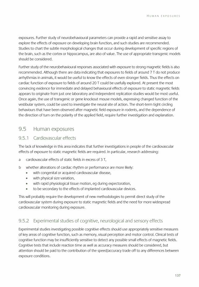
H U M A N E X P O S U R E S
137
exposures. Further study of neurobehavioural parameters can provide a rapid and sensitive assay to explore the effects of exposure on developing brain function, and such studies are recommended. Studies to chart the subtle morphological changes that occur during development of specific regions of the brain, such as the cortex or hippocampus, are also of value. The use of appropriate transgenic models should be considered.
Further study of the neurobehavioural responses associated with exposure to strong magnetic fields is also recommended. Although there are data indicating that exposures to fields of around 7 T do not produce arrhythmias in animals, it would be useful to know the effects of even stronger fields. Thus the effects on cardiac function of exposure to fields of around 20 T could be usefully explored. At present the most convincing evidence for immediate and delayed behavioural effects of exposure to static magnetic fields appears to originate from just one laboratory and independent replication studies would be most useful. Once again, the use of transgenic or gene knockout mouse models, expressing changed function of the vestibular system, could be used to investigate the neural site of action. The short-term tight circling behaviours that have been observed after magnetic field exposure in rodents, and the dependence of the direction of turn on the polarity of the applied field, require further investigation and explanation.
9.5 Human exposures
9.5.1 Cardiovascular effects
The lack of knowledge in this area indicates that further investigations in people of the cardiovascular effects of exposure to static magnetic fields are required. In particular, research addressing:
a cardiovascular effects of static fields in excess of 3 T,
b whether alterations of cardiac rhythm or performance are more likely: • with congenital or acquired cardiovascular disease, • with physical size variation, • with rapid physiological tissue motion, eg during expectoration, • to be secondary to the effects of implanted cardiovascular devices.
This will probably require the development of new methodologies to permit direct study of the cardiovascular system during exposure to static magnetic fields and the need for more widespread cardiovascular monitoring during exposure.
9.5.2 Experimental studies of cognitive, neurological and sensory effects
Experimental studies investigating possible cognitive effects should use appropriately sensitive measures of key areas of cognitive function, such as memory, visual perception and motor control. Clinical tests of cognitive function may be insufficiently sensitive to detect any possible small effects of magnetic fields. Cognitive tests that include reaction time as well as accuracy measures should be considered, but attention should be paid to the contribution of the speed/accuracy trade off to any differences between exposure conditions.
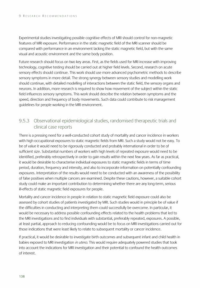
9 R E S E A R C H R E C O M M E N D A T I O N S
138
Experimental studies investigating possible cognitive effects of MRI should control for non-magnetic features of MRI exposure. Performance in the static magnetic field of the MRI scanner should be compared with performance in an environment lacking the static magnetic field, but with the same visual and acoustic environment and the same body position.
Future research should focus on two key areas. First, as the fields used for MRI increase with improving technology, cognitive testing should be carried out at higher field levels. Second, research on acute sensory effects should continue. This work should use more advanced psychometric methods to describe sensory symptoms in more detail. The strong synergy between sensory studies and modelling work should continue, with detailed modelling of interactions between the static field, the sensory organs and neurons. In addition, more research is required to show how movement of the subject within the static field influences sensory symptoms. This work should describe the relation between symptoms and the speed, direction and frequency of body movements. Such data could contribute to risk management guidelines for people working in the MRI environment.
9.5.3 Observational epidemiological studies, randomised therapeutic trials and clinical case reports
There is a pressing need for a well-conducted cohort study of mortality and cancer incidence in workers with high occupational exposures to static magnetic fields from MRI. Such a study would not be easy. To be of value it would need to be rigorously conducted and probably international in order to be of sufficient size. Substantial numbers of workers with high levels of repeated exposure would need to be identified, preferably retrospectively in order to gain results within the next few years. As far as practical, it would be desirable to characterise individual exposures to static magnetic fields in terms of time period, duration, frequency and intensity, and also to incorporate information on potentially confounding exposures. Interpretation of the results would need to be conducted with an awareness of the possibility of false positives when multiple cancers are examined. Despite these cautions, however, a suitable cohort study could make an important contribution to determining whether there are any long-term, serious ill-effects of static magnetic field exposures for people.
Mortality and cancer incidence in people in relation to static magnetic field exposure could also be assessed by cohort studies of patients investigated by MRI. Such studies would in principle be of value if the difficulties in conducting and interpreting them could successfully be overcome. In particular, it would be necessary to address possible confounding effects related to the health problems that led to the MRI investigations and to find individuals with substantial, preferably repeated, exposures. A possible, at least partial, approach to reducing confounding would be to focus on MRI investigations carried out for those indications that were least likely to relate to subsequent mortality or cancer incidence.
If practical, it would be desirable to investigate birth outcomes and subsequent infant and child health in babies exposed to MRI investigation in utero. This would require adequately powered studies that took into account the indications for MRI investigation and their potential to confound the health outcomes of interest.
139
Glossary
GENERAL
Biological effect A measurable change in a biological system in response, for example, to an applied electromagnetic field.
Adverse health effect A biological effect which is detrimental to the mental or physical well-being of exposed individuals, either in the short term or in the long term.
Direct effect A biological effect resulting from direct interaction between a magnetic field and biological structures.
Indirect effect A biological effect resulting from the interaction of a magnetic field with an object other than a person which subsequently has an effect on a person, eg the impact of a metal object on a person when it is caused to accelerate due to magnetic attraction.
BIOLOGY
Accommodation (of nerve) The property of a nerve by which it adjusts to a slowly increasing level of stimulus, so that its threshold of excitation is greater than it would be were the stimulus level to have risen more rapidly.
Action potential (nerve impulse or ‘spike’) A sudden, brief reversal of the local membrane electrical potential that occurs once a threshold depolarisation has been exceeded and which quickly propagates down a nerve axon conveying ‘digitally’ encoded information.
APGAR test A standard method to subjectively measure the physical condition of a newborn infant shortly after delivery.
Central nervous system The cells, such as neurons and glial cells, of the brain and spinal cord. It includes the retina, which is formed as an outgrowth of the forebrain.
Depolarisation A decrease in the value of a cell membrane potential from its normal resting value conventionally described as around –70 mV, the inside of the cell being negative compared to the outside.
Diastole The period of relaxation of heart muscle, following contraction (systole).
Ectopic (heart) beats The term applied to extra heart beats, representing the most common disturbance of heart rhythm.
Fetus (foetus) The stage of prenatal development between the embryo and birth.
G L O S S A R Y
140
Fibrillation (ventricular) Chaotic electrical activity of the ventricles leading to the loss of organised contractions and leading to no useful beating activity.
Gene expression The process whereby the information contained in genes is read and used by cells, usually to make proteins.
Neonate Newly born.
Perfusion rate The rate at which blood flows through the vessels of a specified organ.
Phosphene The perception of flickering patterns of light, usually in the periphery of the visual field, induced by non-visual means such as a trans-retinal electric current.
Synapse A specialised junction between two neurons, or between a neuron and a muscle fibre, that allows the transmission of information, usually by means of the release of a specific chemical (neurotransmitter).
Vestibular system Balance organs of the inner ear.
Voltage-gated ion channel Complex proteins found in a cell membrane that open and close in response to local changes in electrical potential and so allow the passage of selected ions through the cell membrane. They have a key role in the generation and propagation of nerve impulses.
EPIDEMIOLOGY AND STATISTICS
Bias A systematic tendency to overestimate or underestimate a parameter of interest because of a deficiency in the design or execution of an epidemiological study.
Case–control study An epidemiological study in which people who have developed a health outcome (cases) are identified, and their earlier exposure to putative causes is compared with that of controls who have not developed the health outcome.
Cohort (cohort study) An epidemiological study in which people who differ in their exposure to putative determinants of a health outcome are followed up and the subsequent occurrence of the health outcome is compared according to exposure. Cohort studies may be conducted prospectively or retrospectively.
Confidence interval (CI) An interval calculated from data when making inferences about an unknown parameter. In hypothetical repetitions of the study, the interval will include the parameter in question on a specified percentage of occasions (eg 95% for a 95% confidence interval).
Confounding A tendency to overestimate or underestimate the strength of a causal association in an epidemiological study because the putative cause that is under investigation is associated with another variable that independently determines the risk of the health outcome. Confounding can lead to a false conclusion about whether or not there is a causal relationship between exposure and disease.
G L O S S A R Y
141
Cross-sectional study An epidemiological study in which the prevalence of one or more health outcomes and/or their determinants is assessed in a population at a point in time or over a relatively short period.
Odds ratio (OR) The ratio of the odds of a health outcome in people exposed to a risk factor to that in people who are unexposed or exposed at a different level. The odds of a health outcome are defined as p/(1 – p), where p is the probability of the outcome.
Prospective study An epidemiological study in which data on health outcomes are collected as they occur (cf retrospective study).
Relative risk (RR) The ratio of the risk (probability) of a health outcome in people exposed to a risk factor to that in people who are unexposed or exposed at a different level. Relative risks may be estimated with or without adjustment for possible confounding factors, such as age. For rare health outcomes, the relative risk is numerically similar to the odds ratio (see above).
Retrospective study An epidemiological study in which data are collected on health outcomes that occurred before the study began (cf prospective study).
Standardised incidence ratio (SIR) The ratio (often expressed as a percentage) of the number of incident cases of a disease in a study group to the number that would have been expected if, for each combination of sex, age and/or other potential confounding variables) the group had experienced the same incidence as that in a specified standard population (often the national population). An SIR greater than 100 (expressed as a percentage) signifies risk raised in the study group compared with the standard population, and an SIR of less than 100 signifies a reduced risk.
Standardised mortality ratio (SMR) Defined in the same way as an SIR, but with death from a specified cause, rather than incidence of a disease, as the health outcome.
Statistical power The probability that, with a specified degree of statistical confidence, an underlying effect of a given magnitude will be detected in a study. A study with low power might easily fail to detect an important effect, simply by chance.
Statistically significant result A finding in a study that deviates from a stated (or assumed) null hypothesis to an extent that would rarely occur (usually meaning with a probability of less than 5%) simply by chance if the null hypothesis were true.
Proportional mortality ratio (PMR) The ratio (often expressed as a percentage) of the number of deaths in a study group from a specified cause to the number that would have been expected if, for each combination of sex, age and/or other potential confounding variables, the proportion of all deaths that were from that cause was the same as in a specified standard population (often the national population).
G L O S S A R Y
142
PHYSICS AND DOSIMETRY
Attenuation The reduction in amplitude and intensity of a signal, usually measured in units of decibels per unit length of medium (dB m–1) and represented by the attenuation coefficient of the medium in question.
Diamagnetism The magnetisation of a substance which exists only in the presence of an externally applied magnetic field, and in a direction which opposes the external field (see magnetic susceptibility).
Eddy currents Circulating electric currents induced in conducting objects when they are exposed to a time-varying magnetic field. Eddy currents can be induced in biological tissues. In MRI, eddy currents induced in the magnet housing can lead to image artefacts.
Electric field strength (E) The force on a unit of positive charge produced by an electric field. The magnitude of the electric field vector (unit V m–1).
Ferromagnetism The phenomenon by which a material, such as iron, becomes magnetised when placed in an external magnetic field, and remains magnetised when it is no longer in the field (see magnetic susceptibility).
Gradient (magnetic field gradient) A spatial variation in a magnetic field, which is expressed as the rate of change in the field with distance (unit T m−1) in a given direction.
Lorentz force The force exerted on a charged particle in an electromagnetic field. The particle will experience a force due to the electric field and, if it is moving, due to the magnetic field as well.
Magnetic field (strength) A vector quantity, H, specifies a magnetic field at a point in space, and is expressed in amperes per metre (A m–1). The magnitude of the vector is the magnetic field strength.
Magnetic flux density (B) The amount of magnetic flux per unit area of a cross-section, perpendicular to the direction of the flux. It is the product of the magnetic field strength and the permeability of the medium (unit tesla, T).
Magnetic susceptibility A measure of the extent to which a tissue or substance becomes magnetised when placed in a magnetic field.
Paramagnetism The magnetisation which occurs only in the presence of an externally applied magnetic field and in the direction of the applied field (see magnetic susceptibility).
Permeability (μ) The quantity which, when multiplied by the magnetic field strength, gives the magnetic flux density. It indicates the degree of magnetisation in a medium when a magnetic field is applied.
143
Appendix Publications of the independent Advisory Group on Non-ionising Radiation
1 Electromagnetic fields and the risk of cancer. Report of an Advisory Group on Non-ionising Radiation. Doc NRPB, 3(1), 1–138 (1992).
2 Electromagnetic fields and the risk of cancer. Summary of the views of the Advisory Group on Non-ionising Radiation on epidemiological studies published since its 1992 report. Doc NRPB, 4(5), 65–9 (1993).
3 Health effects related to the use of visual display units. Report of an Advisory Group on Non-ionising Radiation. Doc NRPB, 5(2), 1–75 (1994).
4 Electromagnetic fields and the risk of cancer. Supplementary report by the Advisory Group on Non-ionising Radiation (12 April 1994). Doc NRPB, 5(2), 77–81 (1994).
5 Health effects from ultraviolet radiation. Report of an Advisory Group on Non-ionising Radiation. Doc NRPB, 6(2), 7–190 (1995).
6 Use of sunbeds and cosmetic tanning. Statement by the Advisory Group on Non-ionising Radiation. Radiol Prot Bull, No. 218, 11–15 (1999).
7 The solar eclipse. Statement by the Advisory Group on Non-ionising Radiation. Chilton, NRPB Information Services Leaflet P8/99 (1999).
8 ELF electromagnetic fields and the risk of cancer. Report of an Advisory Group on Non-ionising Radiation. Doc NRPB, 12(1), 1–179 (2001).
9 Possible health effects from terrestrial trunked radio (TETRA). Report of an Advisory Group on Non-ionising Radiation. Doc NRPB, 12(2), 1–86 (2001).
10 ELF electromagnetic fields and neurodegenerative disease. Report of an Advisory Group on Non-ionising Radiation. Doc NRPB, 12(4), 1–24 (2001).
11 Health effects from ultraviolet radiation. Report of an Advisory Group on Non-ionising Radiation. Doc NRPB, 13(1), 1–276 (2002).
12 Health effects from radiofrequency electromagnetic fields. Report of an independent Advisory Group on Non-ionising Radiation. Doc NRPB, 14(2), 1–177.
13 Particle deposition in the vicinity of power lines and possible effects on health. Report of an independent Advisory Group on Non-ionising Radiation and its Ad Hoc Group on Corona Ions. Doc NRPB, 15(1), 1–55 (2004).
14 Power frequency electromagnetic fields, melatonin and the risk of breast cancer. Report of an independent Advisory Group on Non-ionising Radiation. Doc HPA, RCE-1, 1–169 (2006).


Health Protection AgencyCentre for Radiation, Chemical and Environmental HazardsChiltonDidcotOxfordshire OX11 0RQUnited Kingdom
Tel: +44(0)1235 831600Fax: +44(0)1235 833891Email: ChiltonInformationOffi [email protected]
Documents of the Health Protection AgencyRadiation, Chemical and Environmental HazardsRCE-6May 2008ISBN 978-0-85951-616-7£32.00© Health Protection AgencyPrinted on chlorine-free paper