Static electric fields unit 2-

Static Electric Fields (UNIT-2)

PREPARED BY GADDALA JAYARAJU, M.TECH

In this chapter we will discuss on the followings:

� Coulomb's Law � Electric Field & Electric Flux Density � Gauss's Law with Application � Electrostatic Potential, Equipotential Surfaces � Boundary Conditions for Static Electric Fields � Capacitance and Capacitors � Electrostatic Energy � Laplace's and Poisson's Equations � Uniqueness of Electrostatic Solutions � Method of Images � Solution of Boundary Value Problems in Different Coordinate Systems.

Introduction

In the previous chapter we have covered the essential mathematical tools needed to study EM fields. We have already mentioned in the previous chapter that electric charge is a fundamental property of matter and charge exist in integral multiple of electronic charge. Electrostatics can be defined as the study of electric charges at rest. Electric fields have their sources in electric charges.

( Note: Almost all real electric fields vary to some extent with time. However, for many problems, the field variation is slow and the field may be considered as static. For some other cases spatial distribution is nearly same as for the static case even though the actual field may vary with time. Such cases are termed as quasi-static.)

In this chapter we first study two fundamental laws governing the electrostatic fields, viz, (1) Coulomb's Law and (2) Gauss's Law. Both these law have experimental basis. Coulomb's law is applicable in finding electric field due to any charge distribution, Gauss's law is easier to use when the distribution is symmetrical.

Coulomb's Law

Coulomb's Law states that the force between two point charges Q1and Q2 is directly proportional to the product of the charges and inversely proportional to the square of the distance between them. Point charge is a hypothetical charge located at a single point in space. It is an idealised model of a particle having an electric charge.



Mathematically, ,where k is the proportionality constant.

In SI units, Q1 and Q2 are expressed in Coulombs(C) and R is in meters.

Force F is in Newtons (N) and , is called the permittivity of free space.

(We are assuming the charges are in free space. If the charges are any other dielectric medium,

we will use instead where is called the relative permittivity or the dielectric constant of the medium).

Therefore .......................(2.1)

As shown in the Figure 2.1 let the position vectors of the point charges Q1and Q2 are given by

and . Let represent the force on Q1 due to charge Q2.

Fig 2.1: Coulomb's Law

The charges are separated by a distance of . We define the unit vectors as

and ..................................(2.2)

can be defined as . Similarly the force on Q1 due to

charge Q2 can be calculated and if represents this force then we can write

When we have a number of point charges, to determine the force on a particular charge due to all other charges, we apply principle of superposition. If we have N number of charges



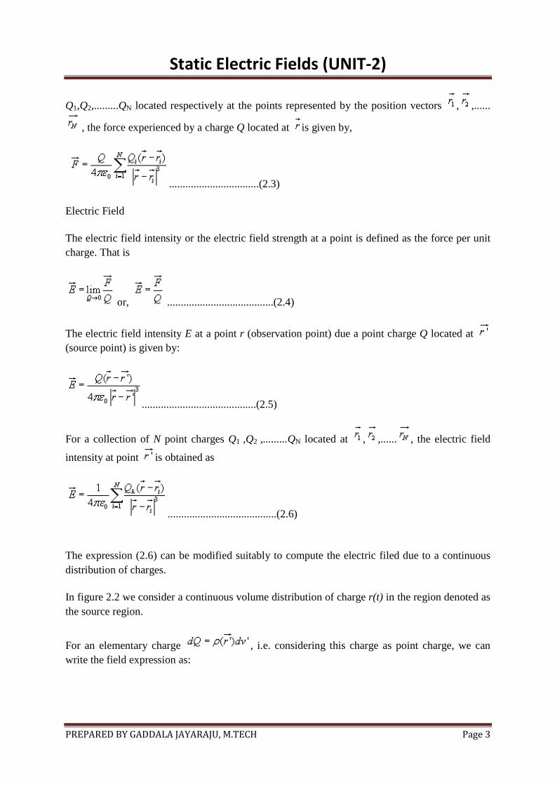
Q1,Q2,.........QN located respectively at the points represented by the position vectors , ,......

, the force experienced by a charge Q located at is given by,

.................................(2.3)

Electric Field

The electric field intensity or the electric field strength at a point is defined as the force per unit charge. That is

or, .......................................(2.4)

The electric field intensity E at a point r (observation point) due a point charge Q located at (source point) is given by:

..........................................(2.5)

For a collection of N point charges Q1 ,Q2 ,.........QN located at , ,...... , the electric field

intensity at point is obtained as

........................................(2.6)

The expression (2.6) can be modified suitably to compute the electric filed due to a continuous distribution of charges.

In figure 2.2 we consider a continuous volume distribution of charge r(t) in the region denoted as the source region.

For an elementary charge , i.e. considering this charge as point charge, we can write the field expression as:



.............(2.7)

Fig 2.2: Continuous Volume Distribution of Charge

When this expression is integrated over the source region, we get the electric field at the point P due to this distribution of charges. Thus the expression for the electric field at P can be written as:

..........................................(2.8)

Similar technique can be adopted when the charge distribution is in the form of a line charge density or a surface charge density.

........................................(2.9)

........................................(2.10)

Electric flux density: As stated earlier electric field intensity or simply ‘Electric field' gives the strength of the field at a particular point. The electric field depends on the material media in which the field is being considered. The flux density vector is defined to be independent of the material media (as we'll see that it relates to the charge that is producing it).For a linear

isotropic medium under consideration; the flux density vector is defined as:



................................................(2.11)

We define the electric flux Y as

.....................................(2.12)

Gauss's Law: Gauss's law is one of the fundamental laws of electromagnetism and it states that the total electric flux through a closed surface is equal to the total charge enclosed by the surface.

Fig 2.3: Gauss's Law

Let us consider a point charge Q located in an isotropic homogeneous medium of dielectric constant e. The flux density at a distance r on a surface enclosing the charge is given by

...............................................(2.13)

If we consider an elementary area ds, the amount of flux passing through the elementary area is given by

.....................................(2.14)

But , is the elementary solid angle subtended by the area at the location of Q.

Therefore we can write

For a closed surface enclosing the charge, we can write



which can seen to be same as what we have stated in the definition of Gauss's Law.

Application of Gauss's Law

Gauss's law is particularly useful in computing or where the charge distribution has some symmetry. We shall illustrate the application of Gauss's Law with some examples.

1.An infinite line charge

As the first example of illustration of use of Gauss's law, let consider the problem of determination of the electric field produced by an infinite line charge of density rLC/m. Let us consider a line charge positioned along the z-axis as shown in Fig. 2.4(a) (next slide). Since the line charge is assumed to be infinitely long, the electric field will be of the form as shown in Fig. 2.4(b) (next slide).

If we consider a close cylindrical surface as shown in Fig. 2.4(a), using Gauss's theorm we can write,

.....................................(2.15)

Considering the fact that the unit normal vector to areas S1 and S3 are perpendicular to the electric field, the surface integrals for the top and bottom surfaces evaluates to zero. Hence we

can write,



Fig 2.4: Infinite Line Charge

.....................................(2.16)

2. Infinite Sheet of Charge

As a second example of application of Gauss's theorem, we consider an infinite charged sheet covering the x-z plane as shown in figure 2.5.

Assuming a surface charge density of for the infinite surface charge, if we consider a

cylindrical volume having sides placed symmetrically as shown in figure 5, we can write:

..............(2.17)



Fig 2.5: Infinite Sheet of Charge

It may be noted that the electric field strength is independent of distance. This is true for the infinite plane of charge; electric lines of force on either side of the charge will be perpendicular to the sheet and extend to infinity as parallel lines. As number of lines of force per unit area gives the strength of the field, the field becomes independent of distance. For a finite charge sheet, the field will be a function of distance.

3. Uniformly Charged Sphere

Let us consider a sphere of radius r0 having a uniform volume charge density of rv C/m3. To

determine everywhere, inside and outside the sphere, we construct Gaussian surfaces of radius r < r 0 and r > r0 as shown in Fig. 2.6 (a) and Fig. 2.6(b).

For the region ; the total enclosed charge will be

.........................(2.18)



Fig 2.6: Uniformly Charged Sphere

By applying Gauss's theorem,

...............(2.19)

Therefore

...............................................(2.20)

For the region ; the total enclosed charge will be

....................................................................(2.21)

By applying Gauss's theorem,

.....................................................(2.22)

Fig. 2.7 shows the variation of D for r0 = 1and .

Electrostatic Potential and Equipotential Surfaces

In the previous sections we have seen how the electric field intensity due to a charge or a charge distribution can be found using Coulomb's law or Gauss's law. Since a charge placed in the vicinity of another charge (or in other words in the field of other charge) experiences a force, the movement of the charge represents energy exchange. Electrostatic potential is related to the work done in carrying a charge from one point to the other in the presence of an electric field.



Let us suppose that we wish to move a positive test charge from a point P to another point Q as shown in the Fig. 2.8.

The force at any point along its path would cause the particle to accelerate and move it out of the region if unconstrained. Since we are dealing with an electrostatic case, a force equal to the

negative of that acting on the charge is to be applied while moves from P to Q. The work

done by this external agent in moving the charge by a distance is given by:

Fig 2.8: Movement of Test Charge in Electric Field

.............................(2.23)

The negative sign accounts for the fact that work is done on the system by the external agent.

.....................................(2.24)

The potential difference between two points P and Q , VPQ, is defined as the work done per unit charge, i.e.

...............................(2.25)

It may be noted that in moving a charge from the initial point to the final point if the potential difference is positive, there is a gain in potential energy in the movement, external agent performs the work against the field. If the sign of the potential difference is negative, work is done by the field.



We will see that the electrostatic system is conservative in that no net energy is exchanged if the test charge is moved about a closed path, i.e. returning to its initial position. Further, the potential difference between two points in an electrostatic field is a point function; it is independent of the path taken. The potential difference is measured in Joules/Coulomb which is referred to as Volts.

Let us consider a point charge Q as shown in the Fig. 2.9.

Fig 2.9: Electrostatic Potential calculation for a point charge

Further consider the two points A and B as shown in the Fig. 2.9. Considering the movement of a unit positive test charge from B to A , we can write an expression for the potential difference as:

..................................(2.26)

It is customary to choose the potential to be zero at infinity. Thus potential at any point ( rA = r) due to a point charge Q can be written as the amount of work done in bringing a unit positive charge from infinity to that point (i.e. rB = 0).

..................................(2.27)

Or, in other words,



..................................(2.28)

Let us now consider a situation where the point charge Q is not located at the origin as shown in Fig. 2.10.

Fig 2.10: Electrostatic Potential due a Displaced Charge

The potential at a point P becomes

..................................(2.29)

So far we have considered the potential due to point charges only. As any other type of charge distribution can be considered to be consisting of point charges, the same basic ideas now can be extended to other types of charge distribution also.

Let us first consider N point charges Q1, Q2,.....QN located at points with position vectors ,

,...... . The potential at a point having position vector can be written as:

..................................(2.30a)

or, ...........................................................(2.30b)

For continuous charge distribution, we replace point charges Qn by corresponding charge

elements or or depending on whether the charge distribution is linear, surface or a volume charge distribution and the summation is replaced by an integral. With these modifications we can write:



For line charge, ..................................(2.31)

For surface charge, .................................(2.32)

For volume charge, .................................(2.33)

It may be noted here that the primed coordinates represent the source coordinates and the unprimed coordinates represent field point.

Further, in our discussion so far we have used the reference or zero potential at infinity. If any other point is chosen as reference, we can write:

.................................(2.34)

where C is a constant. In the same manner when potential is computed from a known electric field we can write:

.................................(2.35)

The potential difference is however independent of the choice of reference.

.......................(2.36)

We have mentioned that electrostatic field is a conservative field; the work done in moving a charge from one point to the other is independent of the path. Let us consider moving a charge from point P1 to P2 in one path and then from point P2 back to P1 over a different path. If the work done on the two paths were different, a net positive or negative amount of work would have been done when the body returns to its original position P1. In a conservative field there is no mechanism for dissipating energy corresponding to any positive work neither any source is present from which energy could be absorbed in the case of negative work. Hence the question of different works in two paths is untenable, the work must have to be independent of path and depends on the initial and final positions.

Since the potential difference is independent of the paths taken, VAB = - VBA , and over a closed path,



.................................(2.37)

Applying Stokes's theorem, we can write:

............................(2.38)

from which it follows that for electrostatic field,

........................................(2.39)

Any vector field that satisfies is called an irrotational field.

From our definition of potential, we can write

.................................(2.40)

from which we obtain,

..........................................(2.41)

From the foregoing discussions we observe that the electric field strength at any point is the

negative of the potential gradient at any point, negative sign shows that is directed from

higher to lower values of . This gives us another method of computing the electric field, i. e. if we know the potential function, the electric field may be computed. We may note here that that

one scalar function contain all the information that three components of carry, the same is

possible because of the fact that three components of are interrelated by the relation .

Example: Electric Dipole

An electric dipole consists of two point charges of equal magnitude but of opposite sign and separated by a small distance.



As shown in figure 2.11, the dipole is formed by the two point charges Q and -Q separated by a distance d , the charges being placed symmetrically about the origin. Let us consider a point P at a distance r, where we are interested to find the field.

Fig 2.11 : Electric Dipole

The potential at P due to the dipole can be written as:

..........................(2.42)

When r1 and r2>>d, we can write and .

Therefore,

....................................................(2.43)

We can write,

...............................................(2.44)

The quantity is called the dipole moment of the electric dipole.

Hence the expression for the electric potential can now be written as:

................................(2.45)



It may be noted that while potential of an isolated charge varies with distance as 1/r that of an electric dipole varies as 1/r2 with distance.

If the dipole is not centered at the origin, but the dipole center lies at , the expression for the potential can be written as:

........................(2.46)

The electric field for the dipole centered at the origin can be computed as

........................(2.47)

is the magnitude of the dipole moment. Once again we note that the electric field of electric dipole varies as 1/r3 where as that of a point charge varies as 1/r2.

Equipotential Surfaces

An equipotential surface refers to a surface where the potential is constant. The intersection of an equipotential surface with an plane surface results into a path called an equipotential line. No work is done in moving a charge from one point to the other along an equipotential line or surface.

In figure 2.12, the dashes lines show the equipotential lines for a positive point charge. By symmetry, the equipotential surfaces are spherical surfaces and the equipotential lines are circles. The solid lines show the flux lines or electric lines of force.



Fig 2.12: Equipotential Lines for a Positive Point Charge

Michael Faraday as a way of visualizing electric fields introduced flux lines. It may be seen that the electric flux lines and the equipotential lines are normal to each other.

In order to plot the equipotential lines for an electric dipole, we observe that for a given Q and d,

a constant V requires that is a constant. From this we can write to be the equation for an equipotential surface and a family of surfaces can be generated for various values of cv.When plotted in 2-D this would give equipotential lines.

To determine the equation for the electric field lines, we note that field lines represent the

direction of in space. Therefore,

, k is a constant .................................................................(2.48)

.................(2.49)

For the dipole under consideration =0 , and therefore we can write,

.........................................................(2.50)

Integrating the above expression we get , which gives the equations for electric flux lines. The representative plot ( cv = c assumed) of equipotential lines and flux lines for a dipole is shown in fig 2.13. Blue lines represent equipotential, red lines represent field lines.



Boundary conditions for Electrostatic fields

In our discussions so far we have considered the existence of electric field in the homogeneous medium. Practical electromagnetic problems often involve media with different physical properties. Determination of electric field for such problems requires the knowledge of the relations of field quantities at an interface between two media. The conditions that the fields must satisfy at the interface of two different media are referred to as boundary conditions .

In order to discuss the boundary conditions, we first consider the field behavior in some common material media.

In general, based on the electric properties, materials can be classified into three categories: conductors, semiconductors and insulators (dielectrics). In conductor , electrons in the outermost shells of the atoms are very loosely held and they migrate easily from one atom to the other. Most metals belong to this group. The electrons in the atoms of insulators or dielectrics remain confined to their orbits and under normal circumstances they are not liberated under the influence of an externally applied field. The electrical properties of semiconductors fall between those of conductors and insulators since semiconductors have very few numbers of free charges.

The parameter conductivity is used characterizes the macroscopic electrical property of a material medium. The notion of conductivity is more important in dealing with the current flow and hence the same will be considered in detail later on.

If some free charge is introduced inside a conductor, the charges will experience a force due to mutual repulsion and owing to the fact that they are free to move, the charges will appear on the surface. The charges will redistribute themselves in such a manner that the field within the

conductor is zero. Therefore, under steady condition, inside a conductor .

From Gauss's theorem it follows that

= 0 .......................(2.51)

The surface charge distribution on a conductor depends on the shape of the conductor. The charges on the surface of the conductor will not be in equilibrium if there is a tangential component of the electric field is present, which would produce movement of the charges. Hence under static field conditions, tangential component of the electric field on the conductor surface is zero. The electric field on the surface of the conductor is normal everywhere to the surface . Since the tangential component of electric field is zero, the conductor surface is an equipotential

surface. As = 0 inside the conductor, the conductor as a whole has the same potential. We may further note that charges require a finite time to redistribute in a conductor. However, this time is

very small sec for good conductor like copper.



Let us now consider an interface between a conductor and free space as shown in the figure 2.14. Fig 2.14: Boundary Conditions for at the surface of a Conductor

Let us consider the closed path pqrsp for which we can write,

.................................(2.52)

For and noting that inside the conductor is zero, we can write

=0.......................................(2.53)

Et is the tangential component of the field. Therefore we find that

Et = 0 ...........................................(2.54)

In order to determine the normal component En, the normal component of , at the surface of

the conductor, we consider a small cylindrical Gaussian surface as shown in the Fig.12. Let

represent the area of the top and bottom faces and represents the height of the cylinder. Once

again, as , we approach the surface of the conductor. Since = 0 inside the conductor is zero,

.............(2.55)

..................(2.56)

Therefore, we can summarize the boundary conditions at the surface of a conductor as:

Et = 0 ........................(2.57)



.....................(2.58)

Behavior of dielectrics in static electric field: Polarization of dielectric

Here we briefly describe the behavior of dielectrics or insulators when placed in static electric field. Ideal dielectrics do not contain free charges. As we know, all material media are composed of atoms where a positively charged nucleus (diameter ~ 10-15m) is surrounded by negatively charged electrons (electron cloud has radius ~ 10-10m) moving around the nucleus. Molecules of dielectrics are neutral macroscopically; an externally applied field causes small displacement of the charge particles creating small electric dipoles.These induced dipole moments modify electric fields both inside and outside dielectric material.

Molecules of some dielectric materials posses permanent dipole moments even in the absence of an external applied field. Usually such molecules consist of two or more dissimilar atoms and are called polar molecules. A common example of such molecule is water molecule H2O. In polar molecules the atoms do not arrange themselves to make the net dipole moment zero. However, in the absence of an external field, the molecules arrange themselves in a random manner so that net dipole moment over a volume becomes zero. Under the influence of an applied electric field, these dipoles tend to align themselves along the field as shown in figure 2.15. There are some materials that can exhibit net permanent dipole moment even in the absence of applied field. These materials are called electrets that made by heating certain waxes or plastics in the presence of electric field. The applied field aligns the polarized molecules when the material is in the heated state and they are frozen to their new position when after the temperature is brought down to its normal temperatures. Permanent polarization remains without an externally applied field.

As a measure of intensity of polarization, polarization vector (in C/m2) is defined as:

.......................(2.59)

n being the number of molecules per unit volume i.e. is the dipole moment per unit volume.

Let us now consider a dielectric material having polarization and compute the potential at an

external point O due to an elementary dipole dv'.



Fig 2.16: Potential at an External Point due to an Elementary Dipole dv'.

With reference to the figure 2.16, we can write: ..........................................(2.60) Therefore,

........................................(2.61)........(2.62) where x,y,z represent the coordinates of the external point O and x',y',z' are the coordinates of the source point.

From the expression of R, we can verify that

.............................................(2.63)

.........................................(2.64)

Using the vector identity, ,where f is a scalar quantity , we have,

.......................(2.65)



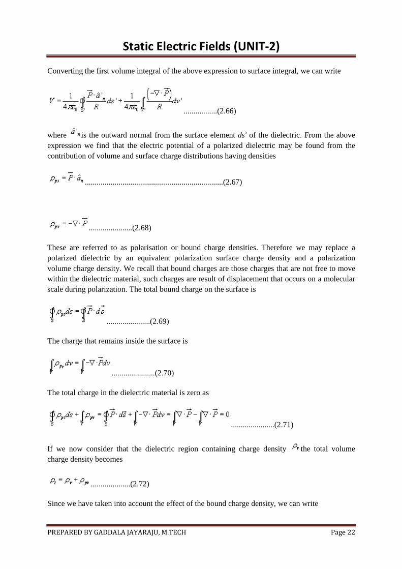
Converting the first volume integral of the above expression to surface integral, we can write

.................(2.66)

where is the outward normal from the surface element ds' of the dielectric. From the above expression we find that the electric potential of a polarized dielectric may be found from the contribution of volume and surface charge distributions having densities

......................................................................(2.67)

......................(2.68)

These are referred to as polarisation or bound charge densities. Therefore we may replace a polarized dielectric by an equivalent polarization surface charge density and a polarization volume charge density. We recall that bound charges are those charges that are not free to move within the dielectric material, such charges are result of displacement that occurs on a molecular scale during polarization. The total bound charge on the surface is

......................(2.69)

The charge that remains inside the surface is

......................(2.70)

The total charge in the dielectric material is zero as

......................(2.71)

If we now consider that the dielectric region containing charge density the total volume charge density becomes

....................(2.72)

Since we have taken into account the effect of the bound charge density, we can write



....................(2.73)

Using the definition of we have

....................(2.74)

Therefore the electric flux density

When the dielectric properties of the medium are linear and isotropic, polarisation is directly proportional to the applied field strength and

........................(2.75)

is the electric susceptibility of the dielectric. Therefore,

.......................(2.76)

is called relative permeability or the dielectric constant of the medium. is called the absolute permittivity.

A dielectric medium is said to be linear when is independent of and the medium is

homogeneous if is also independent of space coordinates. A linear homogeneous and isotropic medium is called a simple medium and for such medium the relative permittivity is a constant.

Dielectric constant may be a function of space coordinates. For anistropic materials, the dielectric constant is different in different directions of the electric field, D and E are related by a permittivity tensor which may be written as:

.......................(2.77)

For crystals, the reference coordinates can be chosen along the principal axes, which make off diagonal elements of the permittivity matrix zero. Therefore, we have



.......................(2.78)

Media exhibiting such characteristics are called biaxial. Further, if then the medium is

called uniaxial. It may be noted that for isotropic media, .

Lossy dielectric materials are represented by a complex dielectric constant, the imaginary part of which provides the power loss in the medium and this is in general dependant on frequency.

Another phenomenon is of importance is dielectric breakdown. We observed that the applied electric field causes small displacement of bound charges in a dielectric material that results into polarization. Strong field can pull electrons completely out of the molecules. These electrons being accelerated under influence of electric field will collide with molecular lattice structure causing damage or distortion of material. For very strong fields, avalanche breakdown may also occur. The dielectric under such condition will become conducting.

The maximum electric field intensity a dielectric can withstand without breakdown is referred to as the dielectric strength of the material.

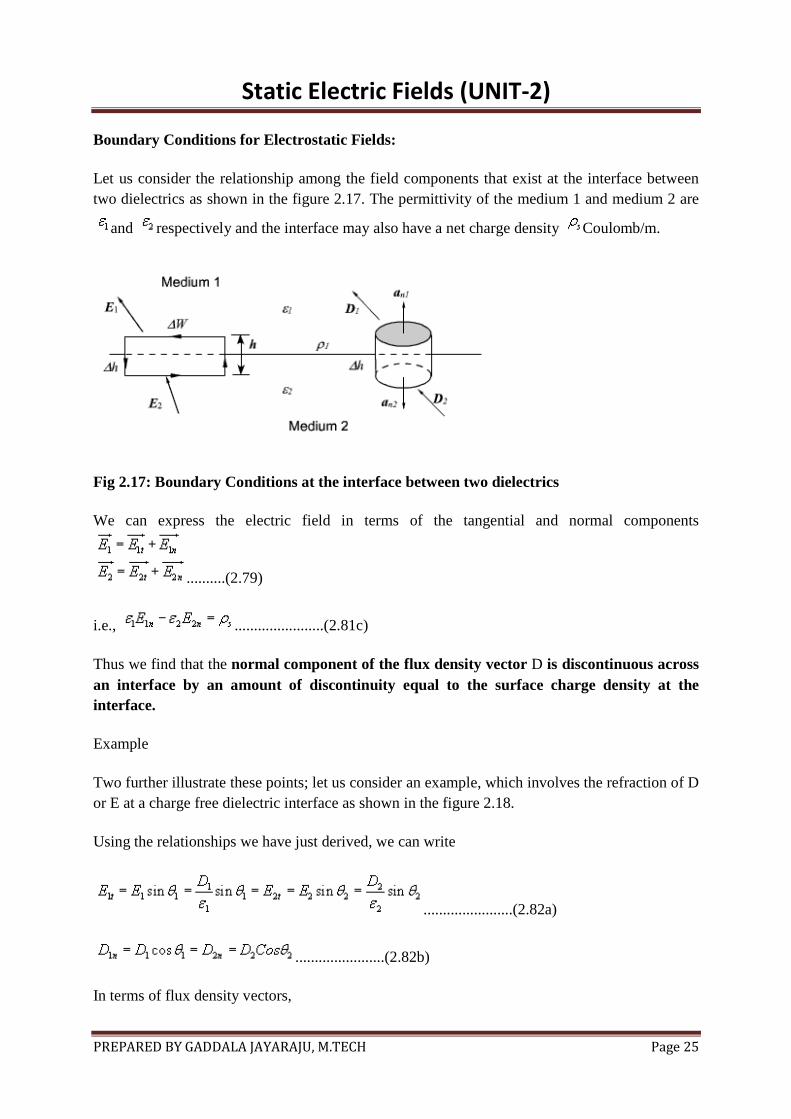
Boundary Conditions for Electrostatic Fields:

Let us consider the relationship among the field components that exist at the interface between two dielectrics as shown in the figure 2.17. The permittivity of the medium 1 and medium 2 are

and respectively and the interface may also have a net charge density Coulomb/m.

Fig 2.17: Boundary Conditions at the interface between two dielectrics

We can express the electric field in terms of the tangential and normal components

..........(2.79)



Boundary Conditions for Electrostatic Fields:

Let us consider the relationship among the field components that exist at the interface between two dielectrics as shown in the figure 2.17. The permittivity of the medium 1 and medium 2 are

and respectively and the interface may also have a net charge density Coulomb/m.

Fig 2.17: Boundary Conditions at the interface between two dielectrics

We can express the electric field in terms of the tangential and normal components

..........(2.79)

i.e., .......................(2.81c)

Thus we find that the normal component of the flux density vector D is discontinuous across an interface by an amount of discontinuity equal to the surface charge density at the interface.

Example

Two further illustrate these points; let us consider an example, which involves the refraction of D or E at a charge free dielectric interface as shown in the figure 2.18.

Using the relationships we have just derived, we can write

.......................(2.82a)

.......................(2.82b)

In terms of flux density vectors,



.......................(2.83a)

.......................(2.83b)

Therefore, .......................(2.84)

Fig 2.18: Refraction of D or E at a Charge Free Dielectric Interface

Capacitance and Capacitors

We have already stated that a conductor in an electrostatic field is an Equipotential body and any charge given to such conductor will distribute themselves in such a manner that electric field inside the conductor vanishes. If an additional amount of charge is supplied to an isolated

conductor at a given potential, this additional charge will increase the surface charge density .

Since the potential of the conductor is given by , the potential of the conductor

will also increase maintaining the ratio same. Thus we can write where the constant of proportionality C is called the capacitance of the isolated conductor. SI unit of capacitance is Coulomb/ Volt also called Farad denoted by F. It can It can be seen that if V=1, C = Q. Thus capacity of an isolated conductor can also be defined as the amount of charge in Coulomb required to raise the potential of the conductor by 1 Volt.

Of considerable interest in practice is a capacitor that consists of two (or more) conductors carrying equal and opposite charges and separated by some dielectric media or free space. The conductors may have arbitrary shapes. A two-conductor capacitor is shown in figure 2.19.



Fig 2.19: Capacitance and Capacitors

When a d-c voltage source is connected between the conductors, a charge transfer occurs which results into a positive charge on one conductor and negative charge on the other conductor. The conductors are equipotential surfaces and the field lines are perpendicular to the conductor surface. If V is the mean potential difference between the conductors, the capacitance is given by

. Capacitance of a capacitor depends on the geometry of the conductor and the permittivity of the medium between them and does not depend on the charge or potential difference between conductors. The capacitance can be computed by assuming Q(at the same

time -Q on the other conductor), first determining using Gauss’s theorem and then

determining . We illustrate this procedure by taking the example of a parallel plate capacitor.

Example: Parallel plate capacitor

Fig 2.20: Parallel Plate Capacitor

For the parallel plate capacitor shown in the figure 2.20, let each plate has area A and a distance h separates the plates. A dielectric of permittivity fills the region between the plates. The



electric field lines are confined between the plates. We ignore the flux fringing at the edges of the plates and charges are assumed to be uniformly distributed over the conducting plates with

densities and - , .

By Gauss’s theorem we can write, .......................(2.85)

As we have assumed to be uniform and fringing of field is neglected, we see that E is constant

in the region between the plates and therefore, we can write . Thus, for a parallel

plate capacitor we have, ........................(2.86)

Series and parallel Connection of capacitors

Capacitors are connected in various manners in electrical circuits; series and parallel connections are the two basic ways of connecting capacitors. We compute the equivalent capacitance for such connections.

Series Case: Series connection of two capacitors is shown in the figure 2.21. For this case we can write,

.......................(2.87)

Fig 2.21: Series Connection of Capacitors



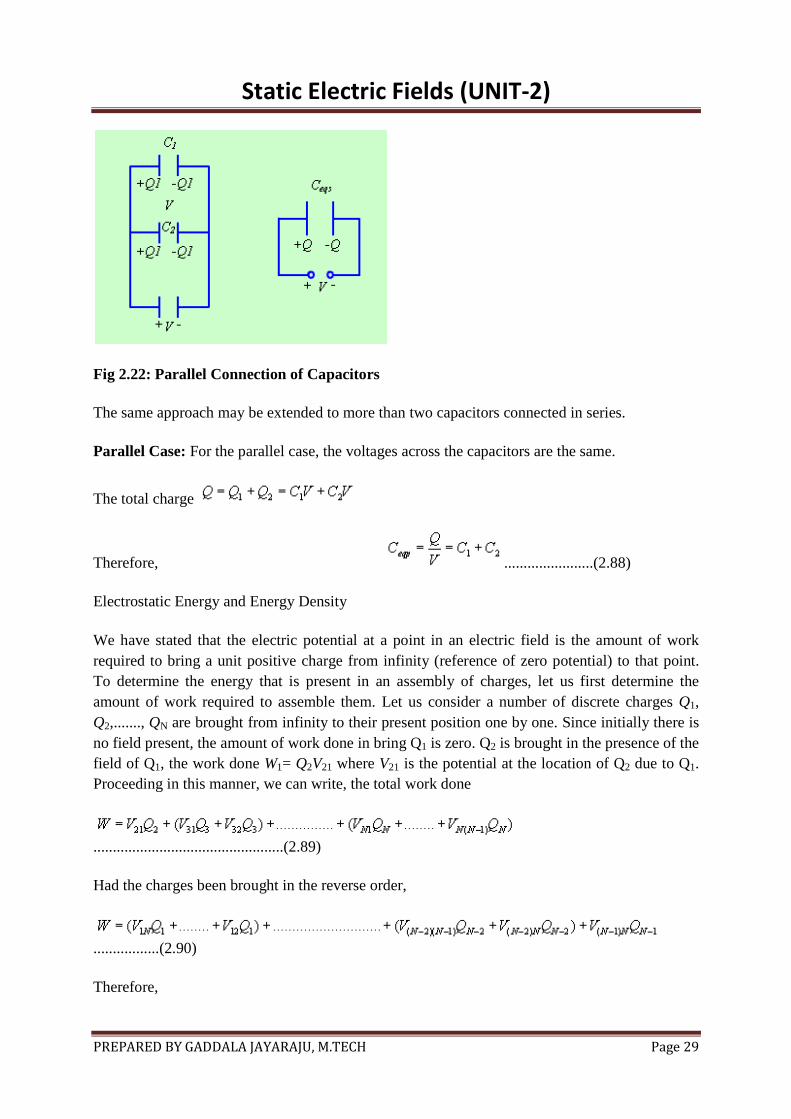
Fig 2.22: Parallel Connection of Capacitors

The same approach may be extended to more than two capacitors connected in series.

Parallel Case: For the parallel case, the voltages across the capacitors are the same.

The total charge

Therefore, .......................(2.88)

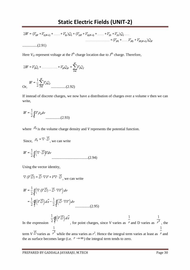
Electrostatic Energy and Energy Density

We have stated that the electric potential at a point in an electric field is the amount of work required to bring a unit positive charge from infinity (reference of zero potential) to that point. To determine the energy that is present in an assembly of charges, let us first determine the amount of work required to assemble them. Let us consider a number of discrete charges Q1, Q2,......., QN are brought from infinity to their present position one by one. Since initially there is no field present, the amount of work done in bring Q1 is zero. Q2 is brought in the presence of the field of Q1, the work done W1= Q2V21 where V21 is the potential at the location of Q2 due to Q1. Proceeding in this manner, we can write, the total work done

.................................................(2.89)

Had the charges been brought in the reverse order,

.................(2.90)

Therefore,



................(2.91)

Here VIJ represent voltage at the I th charge location due to Jth charge. Therefore,

Or, ................(2.92)

If instead of discrete charges, we now have a distribution of charges over a volume v then we can write,

................(2.93)

where is the volume charge density and V represents the potential function.

Since, , we can write

.......................................(2.94)

Using the vector identity,

, we can write

................(2.95)

In the expression , for point charges, since V varies as and D varies as , the

term V varies as while the area varies as r2. Hence the integral term varies at least as and the as surface becomes large (i.e. ) the integral term tends to zero.



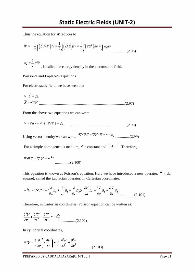
Thus the equation for W reduces to

................(2.96)

, is called the energy density in the electrostatic field.

Poisson’s and Laplace’s Equations

For electrostatic field, we have seen that

..........................................................................................(2.97)

Form the above two equations we can write

..................................................................(2.98)

Using vector identity we can write, ................(2.99)

For a simple homogeneous medium, is constant and . Therefore,

................(2.100)

This equation is known as Poisson’s equation. Here we have introduced a new operator, ( del square), called the Laplacian operator. In Cartesian coordinates,

...............(2.101)

Therefore, in Cartesian coordinates, Poisson equation can be written as:

...............(2.102)

In cylindrical coordinates,

...............(2.103)



In spherical polar coordinate system,

...............(2.104)

At points in simple media, where no free charge is present, Poisson’s equation reduces to

...................................(2.105)

which is known as Laplace’s equation.

Laplace’s and Poisson’s equation are very useful for solving many practical electrostatic field problems where only the electrostatic conditions (potential and charge) at some boundaries are known and solution of electric field and potential is to be found throughout the volume. We shall consider such applications in the section where we deal with boundary value problems.

Uniqueness Theorem

Solution of Laplace’s and Poisson’s Equation can be obtained in a number of ways. For a given set of boundary conditions, if we can find a solution to Poisson’s equation ( Laplace’s equation is a special case), we first establish the fact that the solution is a unique solution regardless of the method used to obtain the solution. Uniqueness theorem thus can stated as:

Solution of an electrostatic problem specifying its boundary condition is the only possible solution, irrespective of the method by which this solution is obtained. To prove this theorem, as shown in figure 2.23, we consider a volume Vr and a closed surface Sr encloses this volume. Sr is such that it may also be a surface at infinity. Inside the closed surface Sr , there are charged conducting bodies with surfaces S1 , S2 , S3,....and these charged bodies are at specified potentials.

If possible, let there be two solutions of Poisson’s equation in Vr. Each of these solutions V1 and V2 satisfies Poisson equation as well as the boundary conditions on S1 , S2 ,....Sn and Sr. Since V1 and V2 are assumed to be different, let Vd = V1 -V2 be a different potential function such that,

........................(2.106)

and ...............(2.107)

............................(2.108)



Thus we find that Vd satisfies Laplace’s equation in Vr and on the conductor boundaries Vd is zero as V1 and V2 have same values on those boundaries. Using vector identity we can write:

...............(2.109)

Using the fact that , we can write

..........................(2.110)

Here the surface S consists of Sr as well as S1 , S2, .....S3.

We note that Vd =0 over the conducting boundaries, therefore the contribution to the surface integral from these surfaces are zero. For large surface Sr , we can think the surface to be a

spherical surface of radius . In the surface integral, the term varies as whereas

the area increases as r2, hence the surface integral decreases as . For , the integral vanishes.

Therefore, . Since is non negative everywhere, the volume integral can be

zero only if , which means V1 = V2. That is, our assumption that two solutions are different does not hold. So if a solution exists for Poisson’s (and Laplace’s) equation for a given set of boundary conditions, this solution is a unique solution.

Moreover, in the context of uniqueness of solution, let us look into the role of the boundary

condition. We observe that, , which, can be written as

. Uniqueness of solution is guaranteed everywhere if or =0 on S.

The condition means that on S. This specifies the potential function on S and

is called Dirichlet boundary condition. On the other hand, means on S. Specification of the normal derivative of the potential function is called the Neumann boundary condition and corresponds to specification of normal electric field strength or charge density. If both the Dirichlet and the Neumann boundary conditions are specified over part of S then the problem is said to be over specified or improperly posed.



Method of Images

Form uniqueness theorem, we have seen that in a given region if the distribution of charge and the boundary conditions are specified properly, we can have a unique solution for the electric potential. However, obtaining this solution calls for solving Poisson (or Laplace) equation. A consequence of the uniqueness theorem is that for a given electrostatics problem, we can replace the original problem by another problem at the same time retaining the same charges and boundary conditions. This is the basis for the method of images. Method of images is particularly useful for evaluating potential and field quantities due to charges in the presence of conductors without actually solving for Poisson’s (or Laplace’s) equation. Utilizing the fact that a conducting surface is an equipotential, charge configurations near perfect conducting plane can be replaced by the charge itself and its image so as to produce an equipotential in the place of the conducting plane. To have insight into how this method works, we consider the case of point charge Q at a distance d above a large grounded conducting plane as shown in figure 2.24.

Fig 2.24

For this case, the presence of the positive charge +Q will induce negative charges on the surface of the conducting plane and the electric field lines will be normal to the conductor. For the time

being we do not have the knowledge of the induced charge density .

Fig 2.25

o apply the method of images, if we place an image charge -Q as shown in the figure 2.26, the system of two charges (essentially a dipole) will produce zero potential at the location of the

conducting plane in the original problem. Solution of field and potential in the region plane (conducting plane in the original problem) will remain the same even the solution is obtained by solving the problem with the image charge as the charge and the boundary condition remains

unchanged in the region .



Fig 2.26

We find that at the point P(x, y, z),

...............(2.111)

Similarly, the electric field at P can be computed as:

...............(2.112)

The induced surface charge density on the conductor can be computed as:

...............(2.113)

The total induced charge can be computed as follows:

...............(2.114)

Using change of variables,



...............(2.115)

Thus, as expected, we find that an equal amount of charge having opposite sign is induced on the conductor.

Method of images can be effectively used to solve a variety of problems, some of which are shown in the next slide.

1.Point charge between semi-infinite conducting planes.

Fig 2.27 :Point charge between two perpendicular semi-infinite conducting planes

Fig 2.28: Equivalent Image charge arrangement



In general, for a system consisting of a point charge between two semi-infinite conducting planes

inclined at an angle (in degrees), the number of image charges is given by .

2.Infinite line charge (density C/m) located at a distance d and parallel to an infinite conducting cylinder of radius a.

Fig 2.29: Infinite line charge and parallel conducting cylinder

Fig 2.30: Line charge and its image

The image line charge is located at and has density . See Appendix 1 for details

3.A point charge in the presence of a spherical conductor can similarly be represented in terms of the original charge and its image.

Electrostatic boundary value problem

In this section we consider the solution for field and potential in a region where the electrostatic conditions are known only at the boundaries. Finding solution to such problems requires solving Laplace’s or Poisson’s equation satisfying the specified boundary condition. These types of problems are usually referred to as boundary value problem. Boundary value problems for potential functions can be classified as:

• Dirichlet problem where the potential is specified everywhere in the boundary



• Neumann problem in which the normal derivatives of the potential function are specified everywhere in the boundary

• Mixed boundary value problem where the potential is specified over some boundaries and the normal derivative of the potential is specified over the remaining ones.

Usually the boundary value problems are solved using the method of separation of variables, which is illustrated, for different types of coordinate systems.

Boundary Value Problems In Cartesian Coordinates:

Laplace's equation in cartesian coordinate can be written as,

...............(2.116)

Assuming that V(x,y,z) can be expressed as V(x,y,z) = X(x)Y(y)Z(z) where X(x), Y(y) and Z(z) are functions of x, y and z respectively, we can write:

..............(2.117)

Dividing throughout by X(x)Y(y)Z(z) we get

.

In the above equation, all terms are function of one coordinate variably only, hence we can write:

...........................................................................(2.118)

kx, ky and kz are seperation constant satisfying

All the second order differential equations above has the same form, therefore we discuss the possible form of solution for the first one only.

Depending upon the value of kx , we can have different possible solutions.



.........................(2.119)

A,B,C and D are constants.

Similarly we have the possible solutions for other two differential equations. The particular solutions for X(x), Y(y) and Z(z) to be used will be chosen based on the nature of the problems and the constants A,B etc are evaluated from the boundary conditions. We illustrate the method discussed above with some examples.

Example 1: As shown in the figure 2.31, let us consider two electrodes, one grounded and the other maintained at a potential V. The region between the plates is filled up with two dielectric layers. Further, we assume that there is no variation of the field along x or y and there is no free charge at the interface.

Fig 2.31

The Laplace equation can be written as:

for which we can write the solution in general form as V= Az+B.

Considering the two regions,

.......................(2.120)

Applying the boundary conditions V=0 for z=0 and V=V0 for z = d, we can write



..................(2.121)

Both the solution should give the same potential at z =a . Therefore,

...........................................(2.122a)

or, ...................................(2.122b)

Another equation relating to A1 and A2 is required to solve for the two constants A1 and A2.

We note that at the dielectric boundary at z = a , the normal component of electric flux density

vector is constant. Noting that , we can write

...........................(2.123a)

or, ..................(2.123b)

Solving for A1 and A2, we find that

..................(2.124a)

.................(2.124b)

Using the above expressions for A1 and A2, we can find and .

Example-2: In the earlier example, we considered a situation where the potential function was a function of only one coordinate. In the figure 2.32 we consider a problem where the potential is a function of two coordinate variables. We consider two number of grounded semi-infinite parallel plate electrodes separated by a distance d. A third electrode maintained at potential V0 and insulated from the grounded conductors is placed as shown in the figure 2.32. The potential function is to be determined in the region enclosed by the electrodes.



Fig 2.32: Potential Function Enclosed by the Electrodes

As discussed above, we can write V(x,y,z) = X(x) Y(y) Z(z). We now construct the solution for V such that it satisfies the stated conditions at the boundary.

We find that V is independent of x. Therefore, X(x) = C1 , where C1is a constant.

Therefore, ..................(2.125)

We observe that the potential has to be equal to V0 at y = 0 and as the potential function becomes zero. Therefore, the y dependence can be expressed as an exponential function. Similarly, since V = 0 for z = 0 and z = d, the z dependence will be a sinusoidal function with kz = k, k being a real number.

Therefore, .....................(2.126)

...............(2.127)

.........................(2.128)

Combining all these terms we can write:

, where C is a constant.

Using the condition that V(y,d) =0, we can write , n=1,2,3,....

For a particular n, . Therefore we can write the general solution as



, where Cns are yet to be determined.

Given that . Therefore . Multiplying both sides by on both sides and integrating from z =0 to z = d we can write,

.....................(2.129)

Using orthogonality conditions and evaluating the integrals we can show that

..................................................(2.130)

The general solution for the potential function can therefore be written as

.........................(2.131) n the region y > 0 and 0< z< d .

Boundary Value Problem in Cylindrical and Spherical Polar Coordinates

As in the case of Cartesian coordinates, method of separation of variables can be used to obtain the general solution for boundary value problems in the cylindrical and spherical polar coordinates also. Here we illustrate the case of solution in cylindrical coordinates with a simple example where the potential is a function of one coordinate variable only.

Example 3: Potential distribution in a coaxial conductor

Let us consider a very long coaxial conductor as shown in the figure 2.33, the inner conductor of which is maintained at potential V0 and outer conductor is grounded.



Fig 2.33: Potential Distribution in a Coaxial Conductor

From the symmetry of the problem, we observe that the potential is independent of variation. Similarly, we assume the potential is not a function of z. Thus the Laplace’s equation can be written as

...................................................(2.132)

Integrating the above equation two times we can write

.....................................................(2.133)

where C1 and C2 are constants, which can be evaluated from the boundary conditions

............................................................(2.134)

Evaluating these constants we can write the expression for the potential as

.......................(2.135)

Furthure, .......................(2.136)

Therefore, ........................(2.137)

If we consider a length L of the coaxial conductor, the capacitance



....................................(2.138)

Example-4: Concentric conducting spherical shells

As shown in the figure 2.34, let us consider a pair of concentric spherical conduction shells, outer one being grounded and the inner one maintained at potential V0.

Considering the symmetry, we find that the potential is function of r only. The Laplace’s equation can be written as:

............(2.139) From the above equation, by direct integration we can write,

...............................(2.140) Applying boundary conditions

................................(2.141) we can find C1 and C2 and the expression for the potential can be written as

: ...........................(2.142) The electric field and the capacitor can be obtained using the same procedure described in Example -3.



Fig 2.34: Concentric conducting spherical shells

ADDITIONAL PROBLEMS SOLVED:

1. Two point charges Q 1and Q2 are located at (3,0,0) and (1,2,0). Find the relation between Q1 and Q2 such that x and y component of the total force on a test charge qi placed at (1,-1,0) are equal.

Solution: The force F1 on q0 due to Q1 is given by

Since x and y component of the total force are equal

Or,

Or,

Or,



2. A line charge of charge density lies along z -axis and a point charge Q0 lies at (0,9,0). Find Q0 so that net force on a test charge located at (0,3,0) is zero.

Solution: We know that for an infinite line charge along z, the field at any radial distance

is given by

In the present case, the test charge is located on the y-axis. Thus the force F1 on the test charge q0 due to the line charge is

The force F2 on q0 due to Q0 is

Given C/m

3. (a) The figure Figure P2.1shows an arc AB of radius 'a' and carrying uniform charge

density C/m lies on the xy plane. Calculate the electric field intensity at point P(0,0,h).

(b) What is the electric field at P due to a ring of radius 'a' carrying C/m if the ring lies on the x y plane with its centre at the origin.



Figure P2.1

Solution :

The electric field at P due to the elementary charge dQ

(b) In the case of the circular ring, we have from part (a)

=0 , =



Alternatively,

Figure P2.2

Using symmetry , for any elementary charge dQ , a symetrical charge dQ' exists , so that

and

4. A circular disc of radius 'a' carries a uniform surface charge density as shown in Figure P2.3. Determine the potential and electric field at a point P(0,0,z) on the axis (z > 0) .



Figure P2.3

Solution : Let us consider an elementary area The charge dQ on this elementary area is given by

The potential at the point P due this elementary charge is given by

The electric field



5.Determine the work done in carrying charge from P1((1,1,-3) to P2(4,2,-3) in an electric

field . Solution :

(a) x = y2 dx = 2y.dy E.dl = y.2y.dy + y2.dy = 3 y2dy

(b) Both points P1 and P2 are on z=-3 plane.Euation of the line joining P1 and P2



6. Assume that a circular tube of radius 'a' and height 'h' is placed on the xy plane with its axis coinciding with z axis. A total charge Q is uniformly distributed on the tube. Determine V and E at a point z>h on the z axis.

Figure P2.4

Total charge = Q

Let us consider a ring of charge consisting of a thin strip of width dz' at a height z'. If we

consider a small length of the strip at an angle . Then the charge

The potential due to the ring



The potential at P(0,0,z)

Substituting t = z - z'

7. Dipole moment is located at the point (1, 1,-2). Determine the potential at a point (3, 4, 2).

Solution : We know that for a dipole moment p, the potential V is given by

Where is the position vector of the dipole centre. Here we have



8.The interface between a dielectric medium having relative permittivity 4 and free space is marked the y = 0 plane. If the electric field next to the interface in the free space region is given

by , determine E field on the other side of the interface.

Solution :Let represents the electric field in the free space and represents the electric field in the dielectric region. Since x & z component of the electric fields are parallel to the interface at y = 0, by continuity of tangential field component

By continuity of the normal component of the flux density vector, we can write

in the dielectric region is given by

V/m.

9. A parallel plate capacitor has a plate area of 1 cm2 and 2mm separation between the plates. The space between the plates is filled with a dielectric whose relative permittivity varies linearly from 2 to 4. Neglecting the fringing effect, what would be the capacitance?



Ans:

10. Consider a cylindrical capacitor as shown in the Figure P2.5. Determine the capacitance neglecting the fringing given that a dielectric material of dielectric constant fills the region and another dielectric material of dielectric constant fills the region .

Figure P2.5

Solution :

We find that electric filed has only component and therefore

If we consider a total charge Q then

where

&

Similarly,



Solution : Let us consider the parallel plate capacitor with area A, separation between the plates'd' & the

permittivity varies from to . The plates are placed at z = 0 and z = d. Given : A = 1 cm2 = 10 -4 m 2 d = 2 mm = 10 -3 m

At any height 'z' from the bottom plate,

The charge density on the plate is

The electric field can be written as

The potential

The capacitance C is given by



Substituting the values, The total potential V = V 1 + V 2

=

=

The capacitance It may be noted that, the same relation can also be derived by considering the series connection of two capacitors formed by the two dielectric regions.

Static electric fields unit 2-

Documents

Transcript of Static electric fields unit 2-