MUS420Introduction to Linear State Space Models

Julius O. Smith III (jos@ccrma.stanford.edu)Center for Computer Research in Music and Acoustics (CCRMA)

Department of Music, Stanford UniversityStanford, California 94305

February 5, 2019

Outline

• State Space Models

• Linear State Space Formulation

• Markov Parameters (Impulse Response)

• Transfer Function

• Difference Equations to State Space Models

• Similarity Transformations

• Modal Representation (Diagonalization)

• Matlab Examples

1

State Space Models

Equations of motion for any physical system may beconveniently formulated in terms of its state x(t):

ft

Input Forces u(t)

∫

Model State x(t) x(t)

x(t) = ft[x(t), u(t)]

where

x(t) = state of the system at time t

u(t) = vector of external inputs (typically driving forces)

ft = general function mapping the current state x(t) and

inputs u(t) to the state time-derivative x(t)

• The function ft may be time-varying, in general

• This potentially nonlinear time-varying model isextremely general (but causal)

• Even the human brain can be modeled in this form

2

State-Space History

1. Classic phase-space in physics (Gibbs 1901)System state = point in position-momentum space

2. Digital computer (1950s)

3. Finite State Machines (Mealy and Moore, 1960s)

4. Finite Automata

5. State-Space Models of Linear Systems

6. Reference:Linear system theory: The state spaceapproachL.A. Zadeh and C.A. DesoerKrieger, 1979

3

Key Property of State Vector

The key property of the state vector x(t) in the statespace formulation is that it completely determines thesystem at time t

• Future states depend only on the current state x(t)and on any inputs u(t) at time t and beyond

• All past states and the entire input history are“summarized” by the current state x(t)

• State x(t) includes all “memory” of the system

4

Force-Driven Mass Example

Consider f = ma for the force-driven mass:

• Since the mass m is constant, we can use momentump(t) = mv(t) in place of velocity (more fundamental,since momentum is conserved)

• x(t0) and p(t0) (or v(t0)) define the state of the massm at time t0

• In the absence of external forces f (t), all future statesare predictable from the state at time t0:

p(t) = p(t0) (conservation of momentum)

x(t) = x(t0) +1

m

∫ t

t0

p(τ ) dτ, t ≥ t0

• External forces f (t) drive the state to arbitrary pointsin state space:

p(t) = p(t0) +

∫ t

t0

f (τ ) dτ, t ≥ t0, p(t)∆= mv(t)

x(t) = x(t0) +1

m

∫ t

t0

p(τ ) dτ, t ≥ t0

5

Forming Outputs

Any system output is some function of the state, andpossibly the input (directly):

y(t)∆= ot[x(t), u(t)]

ft

Input Forces u(t)

∫

Model State x(t)x(t)

y(t)ot

Usually the output is a linear combination of statevariables and possibly the current input:

y(t)∆= Cx(t) +Du(t)

where C and D are constant matrices oflinear-combination coefficients

6

Numerical Integration

Recall the general state-space model in continuous time:

x(t) = ft[x(t), u(t)]

An approximate discrete-time numerical solution is

x(tn + Tn) = x(tn) + Tn ftn[x(tn), u(tn)]

for n = 0, 1, 2, . . . . (Forward Euler)

Let gtn[x(tn), u(tn)]∆= x(tn) + Tn ftn[x(tn), u(tn)]:

u(tn)

x(tn)gt

x(tn + Tn)

z−Tn

• This is a simple example of numerical integration forsolving the ODE

• ODE can be nonlinear and/or time-varying

• The sampling interval Tn may be fixed or adaptive

7

State Definition

We need a state variable for the amplitude of eachphysical degree of freedom

Examples:

• Ideal Mass:

Energy =1

2mv2 ⇒ state variable = v(t)

Note that in 3D we get three state variables(vx, vy, vz)

• Ideal Spring:

Energy =1

2kx2 ⇒ state variable = x(t)

• Inductor: Analogous to mass, so current

• Capacitor: Analogous to spring, so charge

(or voltage = charge/capacitance)

• Resistors and dashpots need no state variablesassigned—they are stateless (no “memory”)

8

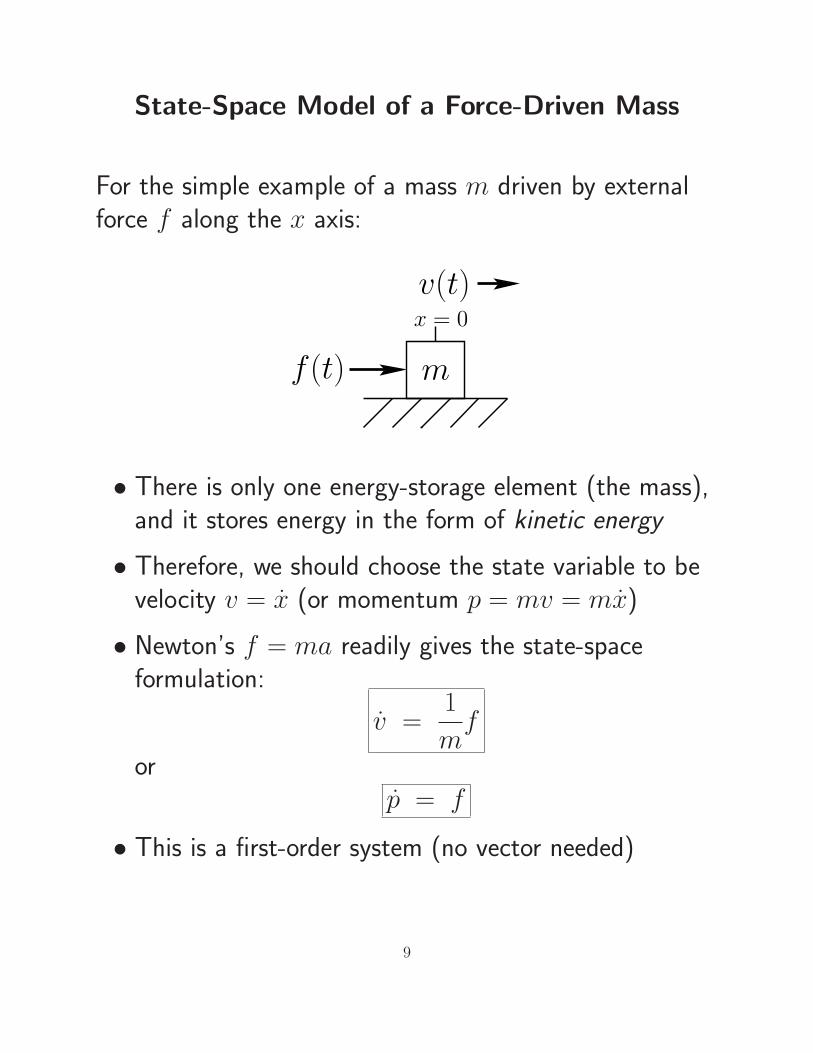
State-Space Model of a Force-Driven Mass

For the simple example of a mass m driven by externalforce f along the x axis:

f (t)

x = 0

v(t)

m

• There is only one energy-storage element (the mass),and it stores energy in the form of kinetic energy

• Therefore, we should choose the state variable to bevelocity v = x (or momentum p = mv = mx)

• Newton’s f = ma readily gives the state-spaceformulation:

v =1

mf

orp = f

• This is a first-order system (no vector needed)

9

Force-Driven Mass Reconsidered

Why not include position x(t) as well as velocity v(t) inthe state-space model for the force-driven mass?

[x(t)

v(t)

]

=

[0 1

0 0

] [x(t)

v(t)

]

+

[0

1/m

]

f (t)

We might expect this because we know from before thatthe complete physical state of a mass consists of itsvelocity v and position x!

10

Force-Driven Mass Reconsidered and Dismissed

• Position x does not affect stored energy

Em =1

2mv2

• Velocity v(t) is the only energy-storing degree of

freedom

• Only velocity v(t) is needed as a state variable

• The initial position x(0) can be kept “on the side” toenable computation of the complete state inposition-momentum space:

x(t) = x(0) +

∫ t

0

v(τ ) dτ

• In other words, the position can be derived from thevelocity history without knowing the force history

• Note that the external force f (t) can only drive v(t).It cannot drive x(t) directly:

[x(t)

v(t)

]

=

[0 1

0 0

] [x(t)

v(t)

]

+

[0

1/m

]

f (t)

11

State Variable Summary

• State variable = physical amplitude for someenergy-storing degree of freedom

• Mechanical Systems:State variable for each

– ideal spring (linear or rotational)

– point mass (or moment of inertia)

times the number of dimensions in which it can move

• RLC Electric Circuits:State variable for each capacitor and inductor

• In Discrete-Time:State variable for each unit-sample delay

• Continuous- or Discrete-Time:Dimensionality of state-space = order of the system(LTI systems)

12

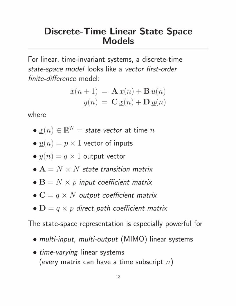
Discrete-Time Linear State SpaceModels

For linear, time-invariant systems, a discrete-timestate-space model looks like a vector first-order

finite-difference model:

x(n + 1) = A x(n) +B u(n)

y(n) = C x(n) +D u(n)

where

• x(n) ∈ RN = state vector at time n

• u(n) = p× 1 vector of inputs

• y(n) = q × 1 output vector

• A = N ×N state transition matrix

• B = N × p input coefficient matrix

• C = q ×N output coefficient matrix

• D = q × p direct path coefficient matrix

The state-space representation is especially powerful for

• multi-input, multi-output (MIMO) linear systems

• time-varying linear systems(every matrix can have a time subscript n)

13

Zero-State Impulse Response(Markov Parameters)

Linear State-Space Model:

y(n) = Cx(n) +Du(n)

x(n + 1) = Ax(n) +Bu(n)

The zero-state impulse response of a state-space model is

easily found by direct calculation: Let x(0)∆= 0 and

u = Ipδ(n) = diag(δ(n), . . . , δ(n)). Then

h(0) = Cx(0)B +DIpδ(0) = D

x(1) = A x(0) +BIpδ(0) = B

h(1) = CB

x(2) = A x(1) +B δ(1) = AB

h(2) = CAB

x(3) = A x(1) +B δ(1) = A2B

h(3) = CA2B

...

h(n) = CAn−1B , n > 0

14

Zero-State Impulse Response (MarkovParameters)

Thus, the “impulse response” of the state-space modelcan be summarized as

h(n) =

{

D, n = 0

CAn−1B, n > 0

• Initial state x(0) assumed to be 0

• Input “impulse” is u = Ipδ(n) = diag(δ(n), . . . , δ(n))

• Each “impulse-response sample” h(n) is a p× qmatrix, in general

• The impulse-response terms CAnB for n ≥ 0 arecalled Markov parameters

15

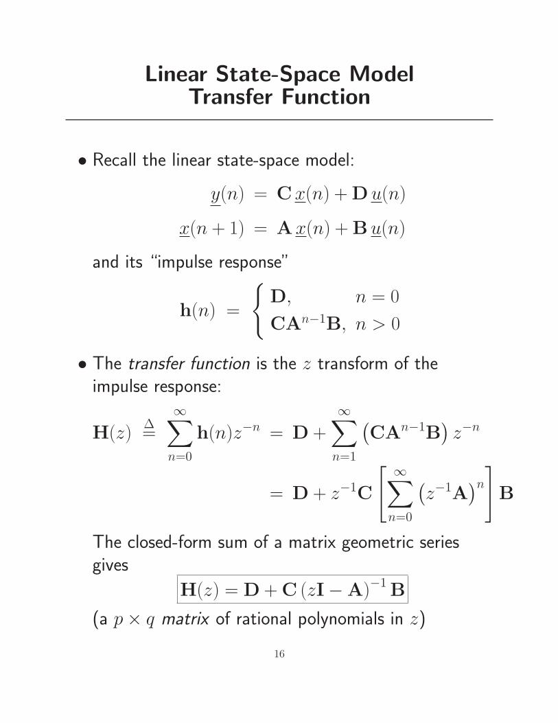
Linear State-Space ModelTransfer Function

• Recall the linear state-space model:

y(n) = C x(n) +Du(n)

x(n + 1) = A x(n) +B u(n)

and its “impulse response”

h(n) =

{

D, n = 0

CAn−1B, n > 0

• The transfer function is the z transform of theimpulse response:

H(z)∆=

∞∑

n=0

h(n)z−n = D +

∞∑

n=1

(CAn−1B

)z−n

= D + z−1C

[ ∞∑

n=0

(z−1A

)n

]

B

The closed-form sum of a matrix geometric seriesgives

H(z) = D +C (zI−A)−1B

(a p× q matrix of rational polynomials in z)

16

• If there are p inputs and q outputs, then H(z) is ap× q transfer-function matrix

(or “matrix transfer function”)

• Given transfer-function coefficients, many digital filterrealizations are possible (different computingstructures)

Example: (p = 3, q = 2)

H(z) =

z−1 1− z−1

1− 0.5z−11 + z−1

2 + 3z−1

1− 0.1z−1

1 + z−1

1− z−1

(1− z−1)2

(1− 0.1z−1)(1− 0.2z−1)

17

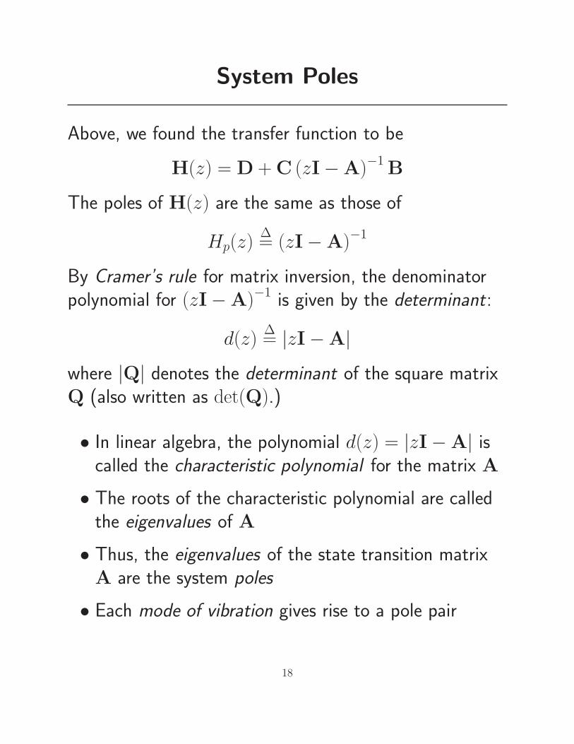
System Poles

Above, we found the transfer function to be

H(z) = D +C (zI−A)−1B

The poles of H(z) are the same as those of

Hp(z)∆= (zI−A)−1

By Cramer’s rule for matrix inversion, the denominatorpolynomial for (zI−A)−1 is given by the determinant:

d(z)∆= |zI−A|

where |Q| denotes the determinant of the square matrixQ (also written as det(Q).)

• In linear algebra, the polynomial d(z) = |zI−A| iscalled the characteristic polynomial for the matrix A

• The roots of the characteristic polynomial are calledthe eigenvalues of A

• Thus, the eigenvalues of the state transition matrixA are the system poles

• Each mode of vibration gives rise to a pole pair

18

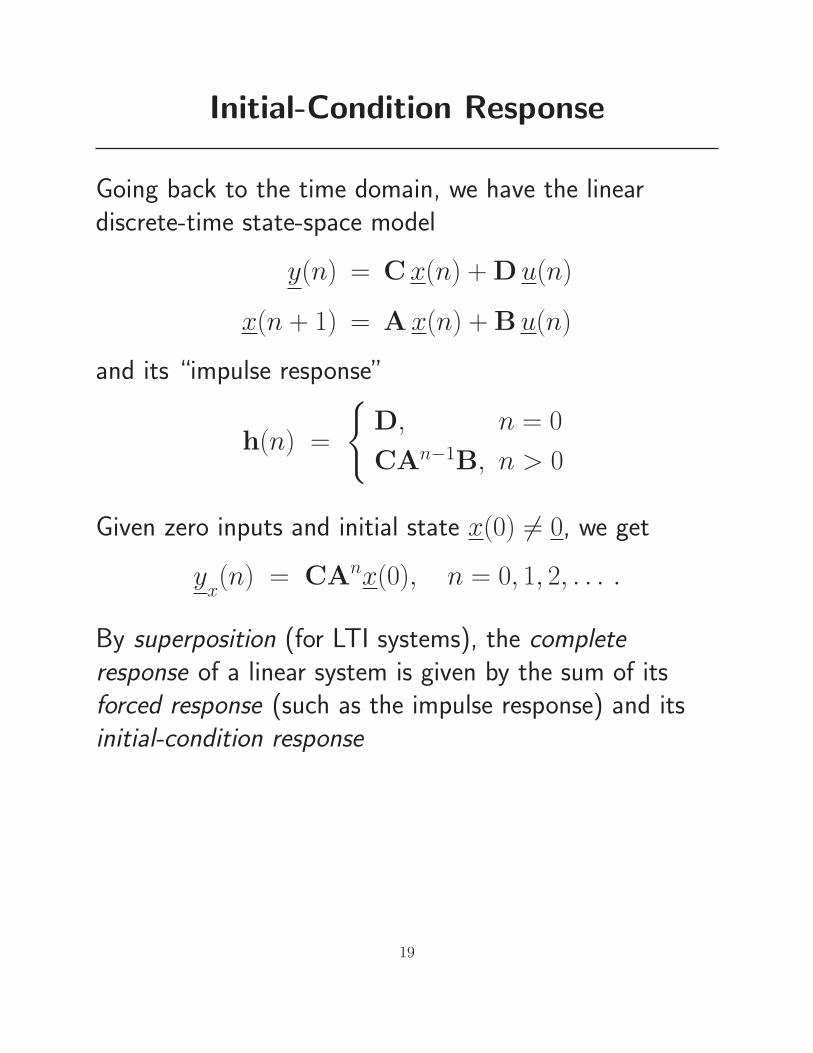
Initial-Condition Response

Going back to the time domain, we have the lineardiscrete-time state-space model

y(n) = C x(n) +D u(n)

x(n + 1) = A x(n) +B u(n)

and its “impulse response”

h(n) =

{

D, n = 0

CAn−1B, n > 0

Given zero inputs and initial state x(0) 6= 0, we get

yx(n) = CAnx(0), n = 0, 1, 2, . . . .

By superposition (for LTI systems), the completeresponse of a linear system is given by the sum of itsforced response (such as the impulse response) and itsinitial-condition response

19

Difference Equation to State Space Form

A digital filter is often specified by its difference equation(Direct Form I). Second-order example:

y(n) = u(n)+2u(n−1)+3u(n−2)−1

2y(n−1)−1

3y(n−2)

Every nth order difference equation can be reformulatedas a first order vector difference equation called the“state space” (or “state variable”) representation:

x(n + 1) = A x(n) +B u(n)

y(n) = C x(n) +D u(n)

For the above example, we have, as we’ll show,

A∆=

[−1

2 −13

1 0

]

(state transition matrix)

B∆=

[1

0

]

(matrix routing input to state variables)

C∆=

[3/2

8/3

]

(output linear-combination matrix)

D∆= 1 (direct feedforward coefficient)

20

Converting to State-Space Form by Hand

1. First, determine the filter transfer function H(z). Inthe example, the transfer function can be written, byinspection, as

H(z) =1 + 2z−1 + 3z−2

1 + 12z

−1 + 13z

−2

2. If h(0) 6= 0, we must “pull out” the parallel delay-freepath:

H(z) = d0 +b1z

−1 + b2z−2

1 + 12z

−1 + 13z

−2

Obtaining a common denominator and equatingnumerator coefficients yields

d0 = 1

b1 = 2− 1

2=

3

2

b2 = 3− 1

3=

8

3

The same result is obtained using long or syntheticdivision

21

3. Next, draw the strictly causal part in direct form II, asshown below:

x(n) y(n)

−1/3

x2(n)

x1(n)

z−1

z−1

3/2

8/3

1

−1/2

x1(n+ 1)

It is important that the filter representation becanonical with respect to delay, i.e., the number ofdelay elements equals the order of the filter

4. Assign a state variable to the output of each delayelement (see figure)

5. Write down the state-space representation byinspection. (Try it and compare to answer above.)

22

Matlab Conversion from Direct-Form toState-Space Form

Matlab has extensive support for state-space models,such as

• tf2ss - transfer-function to state-space conversion

• ss2tf - state-space to transfer-function conversion

Note that these utilities are documented primarily forcontinuous-time systems, but they are also used fordiscrete-time systems.

Let’s repeat the previous example using Matlab:

23

Previous Example Using Matlab

>> num = [1 2 3]; % transfer function numerator

>> den = [1 1/2 1/3]; % denominator coefficients

>> [A,B,C,D] = tf2ss(num,den)

A =

-0.5000 -0.3333

1.0000 0

B =

1

0

C = 1.5000 2.6667

D = 1

>> [N,D] = ss2tf(A,B,C,D)

N = 1.0000 2.0000 3.0000

D = 1.0000 0.5000 0.3333

24

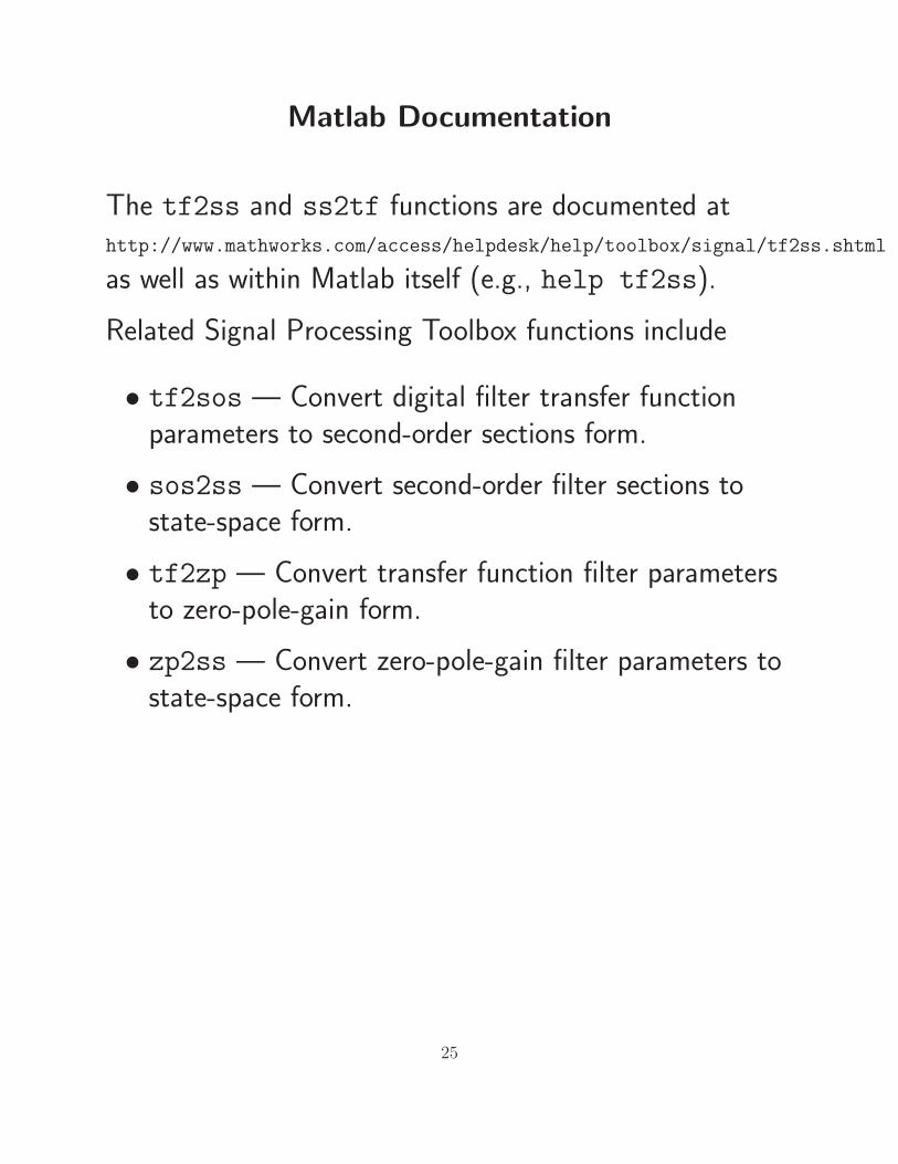
Matlab Documentation

The tf2ss and ss2tf functions are documented athttp://www.mathworks.com/access/helpdesk/help/toolbox/signal/tf2ss.shtml

as well as within Matlab itself (e.g., help tf2ss).

Related Signal Processing Toolbox functions include

• tf2sos — Convert digital filter transfer functionparameters to second-order sections form.

• sos2ss — Convert second-order filter sections tostate-space form.

• tf2zp — Convert transfer function filter parametersto zero-pole-gain form.

• zp2ss — Convert zero-pole-gain filter parameters tostate-space form.

25

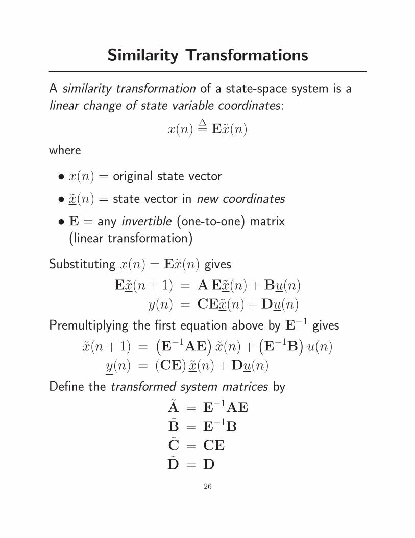
Similarity Transformations

A similarity transformation of a state-space system is alinear change of state variable coordinates:

x(n)∆= Ex(n)

where

• x(n) = original state vector

• x(n) = state vector in new coordinates

• E = any invertible (one-to-one) matrix(linear transformation)

Substituting x(n) = Ex(n) gives

Ex(n + 1) = AEx(n) +Bu(n)

y(n) = CEx(n) +Du(n)

Premultiplying the first equation above by E−1 gives

x(n + 1) =(E−1AE

)x(n) +

(E−1B

)u(n)

y(n) = (CE) x(n) +Du(n)

Define the transformed system matrices by

A = E−1AE

B = E−1B

C = CE

D = D

26

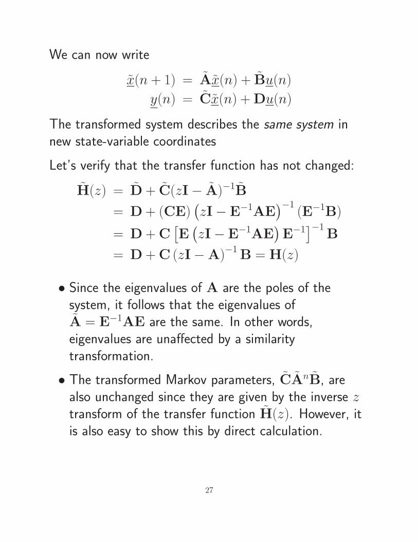
We can now write

x(n + 1) = Ax(n) + Bu(n)

y(n) = Cx(n) +Du(n)

The transformed system describes the same system innew state-variable coordinates

Let’s verify that the transfer function has not changed:

H(z) = D + C(zI− A)−1B

= D + (CE)(zI− E−1AE

)−1(E−1B)

= D +C[E(zI− E−1AE

)E−1

]−1B

= D +C (zI−A)−1B = H(z)

• Since the eigenvalues of A are the poles of thesystem, it follows that the eigenvalues ofA = E−1AE are the same. In other words,eigenvalues are unaffected by a similaritytransformation.

• The transformed Markov parameters, CAnB, arealso unchanged since they are given by the inverse ztransform of the transfer function H(z). However, itis also easy to show this by direct calculation.

27

State Space Modal Representation

Diagonal state transition matrix = modal representation:

x1(n+ 1)

x2(n+ 1).

.

.

xN−1(n+ 1)

xN(n+ 1)

=

λ1 0 0 · · · 0

0 λ2 0 · · · 0.

.

.

.

.

.

.

.

.

.

.

.

.

.

.

0 0 0 λN−1 0

0 0 0 0 λN

x1(n)

x2(n).

.

.

xN−1(n)

xN(n)

+

b1b2.

.

.

bN−1

bN

u(n)

y(n) = Cx(n) +Du(n)

(always possible when there are no repeated poles)

The N complex modes are decoupled :

x1(n + 1) = λ1x1(n) + b1u(n)

x2(n + 1) = λ2x2(n) + b2u(n)...

xN(n + 1) = λNxN(n) + bNu(n)

y(n) = c1x1(n) + c2x2(n) + · · · + cNxN(n) +Du(n)

That is, the diagonal state-space system consists of Nparallel one-pole systems:

H(z) = C(zI−A)−1B +D

= D +

N∑

i=1

cibiz−1

1− λiz−1

28

Finding the (Diagonalized) Modal Representation

The ith eigenvector ei of a matrix A has the definingproperty

Aei = λiei,

where λi is the associated eigenvalue. Thus, theeigenvector ei is invariant under the linear transformationA to within a (generally complex) scale factor λi.

An N ×N matrix A typically has N eigenvectors.1 Let’smake a similarity-transformation matrix E out of the Neigenvectors:

E =[e1 e2 · · · eN

]

Then we have

AE =[λ1e1 λ2e2 · · · λNeN

] ∆= EΛ

where Λ ∆= diag(λ) is a diagonal matrix having

λ ∆=[λ1 λ2 · · · λN

]Talong its diagonal.

Premultiplying by E−1 gives

E−1AE = Λ

Thus, E =[e1 e2 · · · eN

]is a similarity transformation

that diagonalizes the system.1When there are repeated eigenvalues, there may be only one linearly independent eigenvector for the

repeated group. We will not consider this case and refer the interested reader to a Web search on “generalizedeigenvectors,” e.g., http://en.wikipedia.org/wiki/Generalized eigenvector .

29

State-Space Analysis Example:The Digital Waveguide Oscillator

Let’s use state-space analysis to determine the frequencyof oscillation of the following system:

x1(n)

-

x2(n+ 1)

x2(n)x1(n+ 1)

c

z−1 z−1

The second-order digital waveguide oscillator.

Note the assignments of unit-delay outputs to statevariables x1(n) and x2(n).

We have

x1(n+1) = c[x1(n)+x2(n)]−x2(n) = c x1(n)+(c−1)x2(n)

and

x2(n+1) = x1(n)+c[x1(n)+x2(n)] = (1+c)x1(n)+c x2(n)

In matrix form, the state transition can be written as[x1(n + 1)

x2(n + 1)

]

=

[c c− 1

c + 1 c

]

︸ ︷︷ ︸A

[x1(n)

x2(n)

]

30

or, in vector notation,

x(n + 1) = A x(n)

The poles of the system are given by the eigenvalues ofA, which are the roots of its characteristic polynomial.That is, we solve

|λiI−A| = 0

for λi, i = 1, 2, . . . , N , or, for our N = 2 problem,

0 =

∣∣∣∣

λi − c 1− c

−c− 1 λi − c

∣∣∣∣= (λi−c)2+(1−c)(1+c) = λi

2−2λic+1

Using the quadratic formula, the two solutions are foundto be

λi = c±√

c2 − 1 = c± j√

1− c2

Defining c = cos(θ), we obtain the simple formula

λi = cos(θ)± j sin(θ) = e±jθ

It is now clear that the system is a real sinusoidaloscillator for −1 ≤ c ≤ 1, oscillating at normalized radianfrequency ωcT

∆= θ ∆

= arccos(c) ∈ [−π, π].

We determined the frequency of oscillation ωcT from theeigenvalues λi of A. To study this system further, we candiagonalize A. For that we need the eigenvectors as wellas the eigenvalues.

31

Eigenstructure of A

The defining property of the eigenvectors ei andeigenvalues λi of A is the relation

Aei = λiei , i = 1, 2,

which expands to[

c c− 1

c + 1 c

] [1

ηi

]

=

[λi

λiηi

]

.

• The first element of ei is normalized arbitrarily to 1

• We have two equations in two unknowns λi and ηi:

c + ηi(c− 1) = λi

(1 + c) + cηi = λiηi

(We already know λi from above, but this analysiswill find them by a different method.)

• Substitute the first into the second to eliminate λi:

1 + c + cηi = [c + ηi(c− 1)]ηi = cηi + η2i (c− 1)

⇒ 1 + c = η2i (c− 1)

⇒ ηi = ±√

c + 1

c− 1

32

• We have found both eigenvectors:

e1 =

[1

η

]

, e2 =

[1

−η

]

, where η∆=

√

c + 1

c− 1

They are linearly independent providedη 6= 0 ⇔ c 6= −1 and finite provided c 6= 1.

• The eigenvalues are then

λi = c+ηi(c−1) = c±√

c + 1

c− 1(c− 1)2 = c±

√

c2 − 1

• Assuming |c| < 1, they can be written as

λi = c± j√

1− c2

• With c ∈ (−1, 1), define θ = arccos(c), i.e.,

c∆= cos(θ) and

√1− c2 = sin(θ).

• The eigenvalues become

λ1 = c + j√

1− c2 = cos(θ) + j sin(θ) = ejθ

λ2 = c− j√

1− c2 = cos(θ)− j sin(θ) = e−jθ

as expected.

We again found the explicit formula for the frequency ofoscillation:

ωc =θ

T= fs arccos(c),

33

where fs denotes the sampling rate. Or,

c = cos(ωcT )

The coefficient range c ∈ (−1, 1) corresponds tofrequencies f ∈ (−fs/2, fs/2).

We have shown that the example system oscillatessinusoidally at any desired digital frequency ωc whenc = cos(ωcT ), where T denotes the sampling interval.

The Diagonalized Example System

We can now diagonalize our system using the similaritytransformation

E =[e1 e2

]=

[1 1

η −η

]

where η =√

c+1c−1.

We have only been working with the state-transitionmatrix A up to now.

The system has no inputs so it must be excited by initialconditions (although we could easily define one or twoinputs that sum into the delay elements).

34

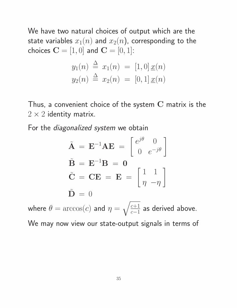
We have two natural choices of output which are thestate variables x1(n) and x2(n), corresponding to thechoices C = [1, 0] and C = [0, 1]:

y1(n)∆= x1(n) = [1, 0] x(n)

y2(n)∆= x2(n) = [0, 1] x(n)

Thus, a convenient choice of the system C matrix is the2× 2 identity matrix.

For the diagonalized system we obtain

A = E−1AE =

[ejθ 0

0 e−jθ

]

B = E−1B = 0

C = CE = E =

[1 1

η −η

]

D = 0

where θ = arccos(c) and η =√

c+1c−1 as derived above.

We may now view our state-output signals in terms of

35

the modal representation:

y1(n) = [1, 0]x(n) = [1, 0]

[1 1

η −η

]

x(n)

= [1, 1]x(n) = λn1 x1(0) + λn

2 x2(0)

y2(n) = [0, 1]x(n) = [0, 1]

[1 1

η −η

]

x(n)

= [η,−η]x(n) = ηλn1 x1(0)− ηλn

2 x2(0)

The output signal from the first state variable x1(n) is

y1(n) = λn1 x1(0) + λn

2 x2(0)

= ejωcnT x1(0) + e−jωcnT x2(0)

The initial condition x(0) = [1, 0]T corresponds to modalinitial state

x(0) = E−1

[1

0

]

=−1

2e

[−e −1

−e 1

] [1

0

]

=

[1/2

1/2

]

For this initialization, the output y1 from the first statevariable x1 is simply

y1(n) =ejωcnT + e−jωcnT

2= cos(ωcnT )

Similarly y2(n) is proportional to sin(ωcnT )(“phase quadrature” output), with amplitude η.

36