Proceedings of The 1980 International Computer Music Conference

John Strawn Center for Computer Research in Music and Acoustics Stanford University Stanford, California 94305

1. Introduction

Of the various models proposed and used for ana­lyzing and synthesizing musical sound, additive synthesis is one of the oldest and best understood. In recent years, time-variant Fourier methods im­plemented as computer programs have made it possible to analyze digitally a large variety of tones from traditional musical instruments. Such re­search has le<l tu a better understanding of the physical and perceptual nature of musical sound as well as improvements in techniques for digital sound synthesis.

The heterodyne filter (Moorer 1973) and the phase vocoder (Portnoff 1976; Moorer 1978) provide time-varying amplitude and frequency functions for each harmonic of a tone being analyzed. This quickly leads to an almost unmanageable increase in the amount of data used to represent the original tone. The question of reducing the amount of data without sacrificing tone quality is thus of potential interest to hardware and software designers as well as musicians and psychoacousticians.

Copyright © l 980 John Strawn.

Computer Music Journal, Vol. 4, No. 3, Fall l980,

116

Approximation and Syntactic Analysis of Amplitude and Frequency Functions-- for Digital Sound Synthesis

One approach to data reduction has involved the use of line-segment approximations (Risset 1969; Beauchamp 1969; Grey 1975), in which an ampli· tude or frequency envelope is represented by a relatively small number of line segments. Depend· ing on the degree of reduction, tones resynthesized using line-segment approximations often sound as though they were produced by the original instru­mental source and in many cases cannot be dis­tinguished perceptually from the original tone.

There is still no definitive answer to the question of how much data can be omitted without changing the tone significantly. The ultimute goal would be to use the smallest possible amount of data to pro­duce a tone that would be perceptually indis­tinguishable from the (digital) recording of the original tone {Strong and Clark 196 7). Grey was un· · able to explore the question of the degree of acceptable data reduction because at that time only analog tape recordings could be digitized for analy­sis by computer at the Center for Computer Re­search in Music and Acoustics f CCRMA). Thus the resynthesized tone could be discriminated from the original tone merely by the absence of tape hiss. Using the digital recording facility (Moorer 19771 it is now possible to record traditional musical instru· ments at CCRMA in digital form.

An important problem in data reduction con· cerns the selection of features to be retained in the

Proceedings of The 1980 International Computer Music Conference

Fig. 1. (a} The amplitude. versus time function of the fifth harmonic of a single trumpet tone, analyzed by the heterodyne filter and normalized to a maximum amplitude of 1.0. The y· axis represents amplitude

0.5

(al

0

r:i' t£. 1500

~ u ! 1250

(bl

0

on an arbitrary linear scale. This fum:,tion has been chosen as an interest­ing test case for investigat· ing methods of approxima­tion because of the large amount of noise in the trace and the presence of

0.25

TI me

0.25

Time

simplified representation of the amplitude and fre· qucncy waveforms. In this article, feature will be used in a very narrow sense to mean components of functions that are presumably important percep· tuallY, An example of this wouid be the so-called blips which typically occur in brass tones, such as those shown in Fig. l (cf. Strong aud Clark 1967; Moorer, Grey, and Strawn 1978). The central hy­pothesis of the work discussed here might be formulated as follows: it is possible to reduce time· varying amplitude and frequency functions derived from traditional instrument tones to some mini­mum number of line segments such that a digitally resynthesized tone using such line segments is per· ceptually indistinguishable (according to some suitable measure! from a digital recording of the original tone. Reducing the number of line seg­ments further, that is, omitting some features, results in tones which can be distinguished from the original.

Various manual and automatic algorithms for

blips in the attack. Pre­sumably such blips play an important role in the timbre of the note from which this function was derived. (b} The frequency­versus-time function for the same harmonic of the

same tone as in (a). Both functions contain 230 points.

- 0.5

0.5

generating line-segment approximations were used in previous research. In the first hall of this paper we will review several algorithms from the litera· ture on pattern recognition which have been developed for analyzing such diverse data as coast­lines on maps (Davis 1977), electrocardiograms {Pavlidis and Horowitz 1974), chromosomes (Fu 1974), outlines of human heads (Kelly 1971), and gasoline blending curves (Stone 1961), but which have not yet been applied to musical problems. After discussing the difficulties inherent in such "low·level11 techniques for the problem at hand, preliminary results from a syntactic, hierarchical scheme for analyzing amplitude and frequency functions will be presented. Since Grey concluded that it was necessary to r~tain time-varying infor· mation for both frequency and amplitude functions (l97SJ, a method for analyzing both will be discussed.

The algorithms which will be outlined below draw extensively from the literature on approxima-

117

Proceedings of The 1980 International Computer Music Conference

tion theory and pattern recognition. Considerations of time and space prevent a review of these topics here, except the mention of some standard texts IDavis 1963; Rosenfeld 1969; Duda and Hart 1973; Fu 1974; Tou and Gonzales 1974) which have proved useful.

The work presented in this article forms part of a larg~r research project investigating the role of tim­bre in the context of a musical phrase. For the purposes of this report, only individual tones from traditional orchestral wind instruments will be pre­sented. The trumpet tone shown in Fig. 1 was analyzed using the heterodyne filter, but the phase vocoder will be used exclusively in future work. No matter which of the two analysis techniques are ap­plied, the issues of approximation remain the same.

2. Line Secments

Formally speaking, the various approximations will be treated as first-degree splines. The following def­inition has been adapted from that of Cox (I 971 ). Let flt) be a sampled function, where t = {to, t 11 t 21

••• tin -11, t"} is a sequence of real numbe!s repre­senting time defined at t = qT; Tis some sampling period and q = 0, 1, 2, .... n. Then a first-degree spline approximation alt) to f(t) is given by

a1(t) = g, + lz.1(t - tao), t E {tao, ta1} alt)= a:z(t) ,_; g:z-. + h:z(t - ta;), t E {ta1 1 ta2} (1)

amlt) =gm + hm(t - ta1m-11)1 t E {ta<m-01 tam}

where m =e;. n, to= tao and tn tam· alt) is also re­quired to be continuous across tao l!li t l!li tam, with continuity defined as

Fig. 2. The solid line repre· sents a /irst·degree spline function a{tl as defined ill Eq. (1). with m = 4. The function f(t) being appmxi· mated is shown as a dot-

ted line. Eacl1 breakpomL of a1 is the same as a point in the origjnal function, as specified in Eq. (3).

For every i E {O .- i ._ m} there exists i E {O ._ i l!li n} such that

The reasons for this restriction will become dear only at the very end of this paper. In the mean· time, it will merely be mentioned again when appropriate.

131

Since the functions being approximated exist only•~ sampled form, such rt!quirements as the ex­isten ;; of the: nth·order derivative are satisfied by definition (see als0 Pavlidis and Maika 1974).

Thete is a considerable body of literature on the use of higher-order approximations, for example cu­bic splines. Line segments, however, have the advantage of being conceptually simple. The effect

Any a1 is obviously continuous across t E {tau-o, ta1}.

IZ) of changing the slope or intercept of a straight line is easy to conceptualize, but it is more difficult to correlate changes in higher-order polynomial coeffi­cients with changes in the appearance of the approximation to some waveform. However, just such a one-to-one correspondence is essential in the feature-oriented work presented here. Cubic splines are also more complicated in that a change in any a(t1) will change all of the coefficients across the entire approximation since the slopes at each t,

Furthermore, one important restriction has been adopted and concerns the endpoints of the line seg­ments used to approximate a function. Each endpoint is required to be the same as some data point in the original waveform (Fig. 2). In terms of the definition given above:

118

Proceedings of The 1980 International Computer Music Conference

are required to be continuous. This criterion of con­tinuity at a breakpoint is in fact ignored when working with line segments. Finally, the line-seg­ment approach is currently implemented in most general-purpose music compilers as well as in most hardware devices for digital sound synthesis.

3. Error Nonns

The most common measure of error is the square of the vertical distance (i.e., the distance parallel to the y-axis! between a function and an approxima­tion to it. Duda and Hart (1973, p. 3321 discuss a variation of this, in which the error is the perpen­dicular distance from a point /{ti of the original function to the approximating line; Dudani and Luk I 1977) present an algorithm for fitting a line to a set of points using this error norm. But according to Moorer { 19801, experience has shown that using this error criterion does not improve the results of approximation for the class of waveforms under dis­cussion here. Since it involves a considerable increase in computation time, this variation has not been tested in the work to be presented below.

Before various methods for approxima:ting func­tions can be examined, three error norms need to be defined.

3.1 Maximum Error

3.3 Mean Squared Error

The mean squared error across each a1 is given by

ta1

I u1t1 - attlP t =tall-II

E111=------ta1 = ta11-11

The Em norm is more tolerant of error across long line segments than the En and E,. norms.

4. Algorithms for Una-Segment Approximation

(6)

There are two basic approaches to solving the prob­lem of approximation using splines. In the first, the number of segments is specified in advance and the algorithm is required to minimize some measure of error. The number of splines is changed in the other method until the measure of error lies as close as possible to, but still under, some predetermined threshold.

4.1 Minimizing Error: ADJUST

One method for minimizing error with a given number of line segments is presented by Pavlidis (1973). Since two typographical errors occurred in Eq. 13) of Pavlidis's article, (which should read PJ = t1!j) - M"'), and since it forms an integral part of the The maximum error E'!C is given by

E.,, = max [i(t) - a{t)] 2, I

(4) procedures discussed in the next section, Pavlidis's algorithm will be discussed in some detail.

with altl deflned in Eq. (11. This is sometimes called the uuiform error norm {Davis 1963, p. 133).

The algorithm, called ADfUST in the rest of this paper, is given in Fig. 3. For each iteration, the endpoints of successive segments !first the odd­numbered segments, then the even-numbered ones) are moved by some number M, always set to 1 in the work discussed in this paper; larger values of M could be specified for the first few iterations if the initial approximation were thought to be signifi­cantly different from the expected final solutiop. If

3.2 Sum-of -Squared Error .

Pavlidis { 19731 also calls this norm the integral square error:

t.

2 [flt) a(t)]2. t=to

(5) the error of the approximation using the trial break­point is less than the original error, then the trial

119

Proceedings ofThe 1980 International Computer Music Conference

Fig. 3. The algorithm AD­/UST. modified from Pavlidis's algorithm (1973), in a quasi-ALGOL nota­tion. The algorithm ac­cepts as input some hmc­tion to be approximated. some initial approxima-

tion a(t) in the form given in Eq. (1). M (the number of points to move n break­point for each tnal). and itcrationLimit (the max­imum number of iterations allowed). When the al­gorithm has finished, ei-

INTEGER itcrationCount, start, stop, i; BOOLEAN odd, breakPointChangcd;

ther iterationlimit has been exceeded or the ap­proximation has been ad-1usted so that any further changes in the breakpoints wm cause some (local) er­ror to increase. Error in this algorithm refers to one

of the three error norms de­fined in Section 3 of the text, although Pavlidis

. originally designed this al­gorithm for the E" and En norms.

FOR iterationCount - l STEP l UNTIL iterationLimit DO BEGIN "iteration loop" brcakPointChanged - FALSE; FOR oJJ - TRUE, FALSE DO

BEGIN "oddicven loop" IF odd THEN start - 1 ELSE start - 2; FOR i - start STEP 2 UNTIL n DO

BEGIN "step through segments" Ti -t111i-lli

T~ - ta;; COMMENT T 1, T2 are the breakpoints for segment ai, T:i - t,.u.,. 11; COMMENT T 2, T:i are the breakpoints for segment a1+1;

e, - error across IT., T2!;

e1.,., - error across IT:i. 73};

IF e, ::;t e1.,. 1 THEN BEGIN "try moving point" IF e1 > e1+1 THEN T/-T~-M ELSE T/-T2+M; e/ - error across (71, T/)i e1+ 1' - error across (T/, T,.); IF MAXIMUM (e1, e1.,..) > M/.xIMUM (e/, e; ... 1') THEN

BEGIN "accept moved point" ta1 ... ::T.j; . breakPointChanged-TRUE; END "accept movt:d point";

END "try moving point"; END "step through segments";

END "odd/even loop"; IF breakPointChanged = FALSE THEN DONE;

END ''iteration loop",

breakpoint replaces the original breakpoint. Pavlidis presents a proof to show that the algorithm will converge in a finit~ number of steps, and lmorc importantly) that no cycling is possible. It must be emphasized that this algorithm is useful for finding local minima, not some globally optimal solution. Pavlidis states that the maximum error norm is to be preferred for most applications, althou&h the sum-of-squared error and mean squared error norms have also been used successfully in the work presented here.

A note on the implementation of ADJUST: if both endpoints of some a1 arc points from the func­tion being approximated, then e1, for example, only

needs to be calculated using points T1+ 1 through T2- l, because the points T 1 and T 2 cannot contribute to the error. This represents a slight improvement over Pavlidis's algorithm, which points out this computational saving only for the beginning endpoint.

The results of applying ADJUST to two test cases are given in Fig. 4 and Table l. The "worst" case {in terms of computational time) is given if the break· points for the original approximation are all gathered at one end of the function, in which case ADJUST must spread the points out across the function in the process of finding the optimal approximation.

120

Fig. 4. Results of applyirig the algorithm AD/UST (given in Fig. 3) to the ap­proximation of two test cases; further data is given in Table l. The En norm was used in all of the cases illustrated here.

0 25

0 25

0 25

Proceedings of The 1980 International Computer Music Conference

(a) This test case consists of two diagonal lines, each corresponding to 24 units on the x-axis, separated by a horizontal line one unit in length. The original smooth diagonal lines have been modified by

50

50

50

adding quasi-random vari­ations, the amplitude of which depends on the y-value of the original line. (b) Arbitrary, initial place­ment of four line seg­l]lents approximating test case (a). (c) Approximation to test case (a), with four line seg­ments. after algorithm AD­/UST has reached a solution. (d) As in (c), but with 11 line segments. Perhaps if the breakpoints were dis­tributed more evenly, the error could be reduced fur-

0

0

0

121

25

25

25

ther and the blip on the left-hand side might be avoided. But AD/UST con­verges onto a locally opti­mal solution, wliich is not necessarily optimal globally. (e) One-half of a sine wave, again spread across 49 units of the x-axis and with 11oise added as in (a). (f) Approximation to (e), with four line segments, after AD/UST has reached a solution. (g) As in (f), with 11 line segments.

so

so

so

Proceedings of The 1980 International Computer Music Conference

Table I. Performance of the algorithm ADJUST for the test cases shown in Fig. 4 Corresponding Illustration in Fig. 4

b, c d f g

Initial 122.9 43.2 0.45 0.0205

Error (E,.)

Final 43.21 25.5 0.o7 0.0190

Number of Iterations

4 2

l1 6

Non: Initial error refers to the error for the initial, arbitrary placement of the approximating line segments. E. is calculated across the entire test case. Note that the function in Figs. 4(al-4(dl varies from 0 to 24, whereas the half-period of the sinusoid in figs. 4(£) and 4(gl does not exceed l .O.

4.2. Initial Segmentation

Three algorithms land a variant of one of them) for approximating a function with line segments will be discussed. The first two represent solutions to the problem, discussed above, of find ng an approx­imation such that the error does not exceed some threshold, with no a priori restrictions on the final number of segments. ·

One widely. used method, in which each line segment provides the least mean squared error approximation to all or part of a function, is not considered here because of the restriction of Eq. 13). Another interesting approach !Stone 1961; Phillips 1968; Pavlidis 1971) will be omitted here for the same reason.

4.2.1 Thresholding Sum-of-Squared Error

The sum-of-squared error norm was defined in Eq. (5). The method, as suggested by Pavlidis j 1973), is quite simple. The endpoint for the approximating segment is incremented until the sum-of·s4uared error exceeds some threshold. The endpoint is then decremented by 1, a segment is established, and the process is repeated using the endpoint just found as the new initial point.

4.2.2 Split-and-Merge

Pavlidis and Horowitz (1974) developed a highly efficient algorithm, presented in Fig. 5. In the ver·

sion to be discussed here, the error across each segment of the approximating function must not exceed some threshold. The initial line segments are first split into smaller line segments until the threshold requirement is satisfied !or the line seg­ment consists of only two points). Neighboring line segments are then joined when possible by MERGE, that is when joining them will not violate the same threshold conditions. FinaJJy, ADJUST is applied to the segmentation. The algorithm repeats until no changes are made to the breakpoints dur· ing an iteration.

In its original formulation, the split-and-merge algorithm returned to the SPLIT procedure {"start:" in Fig. 5[a]) after every iteration. But given the re­striction of Eq. 13), SPLIT only needs to be invoked once {during the first pass) for the following reason. After SPLIT, the error across each segment is less than or equal to the threshold. MERGE likewise can only result in segments with error less than or equal to the threshold. For T./ in ADJUST Id. Fig. 3) to be accepted as a breakpoint, e/ and e1+1' must be less than or equal to e1 and e1+ 1 respectively. But when ADJUST is invoked after MERGE, e, and e1+1

must be less than or equal to the threshold. Thus MERGE and ADJUST cannot result in segments with an error greater than the threshold, so that there is no need to invoke SPLIT again.

4.2.3 "Case 2"

There is another version of the algorithm, called "Case 2" by Pavlidis and Horowitz {19741, in which the error across all of the segments must not ex­ceed some threshold. For the maximum error norm, both cases are identical. When using the sum-of­squared error norm, however, the sum of the squared error across the entire function is exam­ined. Modifications to the split-and-merge al· gorithm are necessary. This variation has been tested but will not be discussed here for reasons to be summarized in Section 4.3.

4.2.4 Curvature

There is yet another method, based on a measure of curvature (Symons 1968; Shirai 1973; 1978). In a · study of human visual perception, Attneave I 1954)

122

Proceedings of The 1980 International Computer Music Conference

Fig. 5. The split-and-merge algorithm in a quasi-AL­GOL notation, after Pavlidis and Horowitz (1974). Procedure ADJUST

is presented in Fig. 3. (a) Outline of the algorithm. {b) Procedure SPLIT. As­sume that SPLIT has been initialized so that ta1 =ta••

al Split-and-Merge Algorithm start: brcakPointChanged - FALSE;

invoke SPLIT loop I: brcakPointChanged ,._ FALSE;

invoke MERGE. invoke one iteration of ADJUST

that is, there is initially one line segment which covers the entire function f(tJ. {c) Procedure MERGE.

IF ibrcakPoint changed by ADJUST or MERGEi TifEN GOTO loop I, ELSE DONE;

bJ Procedure "SPLIT" i - l numberSegments -11 loopl: T1 t- tuo-u; T:i <- l:ai; COMMENT T,, T;i are the breakpoints for segment a0

e.i - error across jT1, r;il; IF e1 > threshold TifEN

BEGIN "split a," IF maximum squared error across (T,, r:1I occurs only once

IBEN Ti - point halfway between (r,, T,) ESLE T2 <-point halfway between (first) two error maxima across {T,, T,.J;

redefine segment a1 to extend from T, to Ti

after a,, insert a new segment to extend from T t to T:t

renumber segments numberSegments -numberSegments+ l; brcakPointChangcd <-TRUE; END "split a/'

ELSE BEGIN COMMENT note that a1 may be split more than once if necessary; i-i+ l IF i > numberSegments IBEN DONE "SPLIT''; END;

GOTO loop2;

cl Procedure "MERGE" i-1;

loop3: IP numberSegments = I TifEN DONE "MERGE"; T1 .-t,1fi-Ui

T,. - tn•I, u; COMMENT segments a, and a1, 1 lie between r, and T:i;

e1 .. - error across (r,, r,,1; IF e, .;; threshold THEN

BEGIN redefine segment a, to extend from T, to T~ ji.e. remove t.,1 as a breakpoint) renumber segments breakPointChanged - TRUE; numberScgments <-- numbcrScgments - I; END

ELSE BEGIN i-i +I; IF i ;;. numberSegments TI-IEN DONE "MERGE"; END;

GOTOloopJ;

123

Proceedings of The 1980 International Computer Music Conference

Fig. 6. (a) Cmvawre (in de­grees) of the waveform show11 in Fig. 1, with M (see text) set to correspond to approximately 12.5 msec. (b) As in (a). but

(a)

50'

0

0

100' (bl

0

100'

0

0

with M = 25 msec. (c) As in (a). with M 50 msec. Jn (a). even small varia­tions in the original func­tion result i11 large values of curvature. Min (c) is so

0.25

0.25

found that the points on a curved line where its di­rection changes most rapidly were extracted by test subjects as endpoints for drawing an outline of the curve. Conversely, he found that an illustration can be satisfactorily reproduced by drawing straight lines between points of high curvature; the cat­drawing in his article has been widely reprinted !e.g., Duda and Hart 1973, p. 339).

Shirai defines curvature at a point P along a digi­tized function as the angle a between RP and PQ, where Q and R are points of the function a constant

large that die puims of high curvature at t ""0.1 sec and t = 0.15 sec are missed.

0.5

0.5

0.5

number of samples (caUed M by Shirai) away from P. In this method, then, the curvature at each point of the function to be approximated is calculated !Fig. 6), and breakpoints are assigned at points of high curvature. If RPQ is a straight line, a = D°; for a highly acute angle RPQ a approaches 1800.

It is important to choose an appropriate value for M. Too small a value will result in distortions in the approximation because features which are too small will cause large variations in curvature and thus be assigned breakpoints. If M is too large, sig-

124

Proceedings of The 1980 International Computer Music Conference

Fig. 7. (a) Approximation to the waveform of Fig. 1, derived from the curvature shown in Fig. 6(b), with the threshold for establish­ing a breakpoint set at 6<r.

The breakpoint which pre­sumably should occur near t = 0.25 sec is missed. (b) As in (a), with a threshold of 3D°. The breakpoint omitted in (a) is included,

0.25

Time

0.25

Time

nificant points of high curvature will be missed (cf. Fig. 7j.

Shirai suggests a thresholding scheme for assign­ing breakpoints according to curvature. This method undoubtedly works for the cases cited by Shirai, in which fairly smooth lines change direc­tion only occasionally. But as is shown in Fig. 7, it seems difficult to find a single threshold which pro­vides a useful approximation for the kinds of functions under consideration here. This method has also been found to be sensitive to the absolute values used to represent /(t), especially for small M. Another problem occurs because the curvature near a probable breakpoint often docs not reach a peak, but rather stays at a plateau; this happens, for ex­ample, at t = 0.1 sec in Fig. 6(b). Obviously only one point needs to be assigned-but which one? I have spent considerable time and effort in an at­tempt to deri vc heuristics for selecting only appropriate peaks of curvature, with no notable success to date. Perhaps a varying curvature thresh-

along with a large amount of presumably extraneous points. The approximation in (a) comprises 32 seg­ments; (b) has 77, both with a long segment for

the initial silence. Choos­ing an appropriate thresh­old would be ;ust as hard, if not harder, for the plots of curvature in Figs. 6(a) and 6(c).

0.5

0.5

old could be applied, but this has not yet been explored.

4.3 Su~mary

Three different analyses using the split-and-merge algorithm arc presented in Fig. 8. As one would ex­pect, the approximation using a very small thresh­old captures many details; as the threshold is in­creased, some details are lost and the overall shape of the waveform is emphasized.

Similar analyses have been conducted using the ''Case 2" form of the split-and-merge algorithm as well as the thresholding algorithm of Section 4.2.1. The mean squared error and maximum squared er- · ror norms have likewise been explored. In general, using any combination of these algorithms and er­ror criteria it is possible to produce results similar to those shown in Fig. 8. Each combination admit­tedly reacts to changes in the threshold in a unique

125

Proceedings of The 1980 International Computer Music Conference

Fig. 8. Results of the split­and-merge algorithm in the form given in Fig. S, usillg the sum-of-squared error norm given by Eq. (5). Recall that the maximum amplitude has been IJor-

!al

4.1 -0

.E 0.5 Q. E <

0

0

(b)

4.1 "'O B

1- 0.5

<

0

0

u "'O a .:= a 0.5 <

0

0

malized to 1. 0. (a) A threshold of 0.001 yields 61 segments. some of which contain otlly two points of the original data. (b) Threshold = 0.01, re· . sulting in 22 segments, a

0.25

Time

0.25

Time

0.25

Time

way, but it seems impossible to reach any general conclusion about the superiority of any algorithm or error norm for the purposes of the work outlined in the introduction to this article.

Rather, it has proven impossible to find a para­digm for controlling the threshold for the one waveform shown here so that the projected percep­tually salient features {e.g., blips in the attack) can be retained or removed without concomitant, sig-

few of which are still only two points long. (c) Twelve segments are found when the threshold 0.05; tlie shortest segment uow covers five points of tbe original data. When the

•

threshold is raised to 0.1 (not shown), the first blip in the attack is missed completely. See Sect.ion 4.3 for further discussion.

0.5

0.5

0.5

nificant changes in the rest of the waveform. If the threshold is large, then the analysis delivers the overall waveshape; with a small threshold, sup­posedly necessary details are retained along with presumably superfluous ones. (Moorer [1980] has suggested that the threshold could be dynamically adjusted according to some measure of randomness, but this approach has not yet bet."tl explored.)

In general, our experience has Jed to the con-

126

Proceedings of The 1980 International Computer Music Conference

clusion that no single algorithm of this type will ultimat.ely be sufficient for the systematic explora· tion of timbre and data reduction. None of these algorithms can take into account both global and local considerations, which seems to be a major drawback. Still, these methods will probably be useful in a wide variety of musical .applications where such control is not a prime consideration.

5. Syntactic Analysis

Hierarchical syntactic analysis would seem ideal for mediating between global and local considera· tions. In the rest of this paper, then, such an approach will be presented.

5.1 Introduction

The method to be discussed draws extensively from the literature on pattern recognition through syn· tactic analysis, which is based on the similarities between the structures of patterns and (formal) lan­guages. There are, of course, many other methods of pattern recognition, such as template matching, but they will not be discussed here.

In syntactic pattern recognition, a rcJatively small vocabulary of terminals, called primitives, is "parsed" according to the rules (productions) of a grammar to form higher-level nonterminals known as "subpatterns" and "features." Characteristic fea­tures are further grouped into patterns (or objects). A successful parse is equated with "recognition" of the pattern. Fortunately, many of the problems in­volved in pattern recognition by computer can be ignored here. A considerable body of literature is devoted, for example, to the question of finding lines in digitized pictures.

5.2 Primitives

One major advantage of syntactic analysis lies in the fact that a relatively small vocabulary of primi­tives can be used for constructing a wide variety of patterns. The choice of primitives is thus an impor-

tant issue. It would seem reasonable, for example, to require that the same primitives be used in the analysis of both amplitude and frequency functions even if it turned out that analysis of the two at higher levels followed different rules.

A generalized approach to primitive !iClection has not yet been found. Fu, however, gives the follow· ing two requirements to serve as guidelines:

(i) The primitives should serve as basic pattern elements to provide a compact but adequate description of the data in terms of the specified structural relations {e.g., the concatenation relation). {iii The primitives should be easily extracted or recognized by existing nonsyntactic meth· ods, sinee they are considered to be simple and compact patterns and their structural informa· tion not important (Fu 1974, p. 47).

Various kinds of primitives have been developed for different pattern-recognition applications. Fu gives many examples, such as Freeman's chain code and half-planes in the pattern space for representing ar· bitrary polygons. However, in light of the restric· tion (still to be justified) imposed in Eq. (3), it seems reasonable to use very small line segments connecting points of the original data as primitives for syntactic analysis.

For reasons discussed by Moorer (1976), the im­plementation of the phase vocoder used at CCRMA performs an averaging of the amplitude and fre· quency functions. At a sampling rate of, for example, 25.6 kHz, 32 samples of the original out­put !corresponding to 1.25 msec) might be averaged to form one output point. These averaged output points are perfectly suited to serve as breakpoints for line-segment primitives in syntactic analysis, and will be used as such in this paper.

5.3 Grammar

The choice of primitives having been made, the next step is to decide on a set of subpatterns and features, a"nd to specify a grammar for parsing the primitives accordingly. Davis and Rosenfeld I l 978) provide a grammar based on hierarchical relaxation

127

Proceedings of The 1980 International Computer Music Conference

methods. Briefly, a line-segment primitive is classi­fied as having length x or 2x, and as being hori· zontal, sloped upward, or sloped downward. The relaxation algorithm parses the primitives into longer line segments at a first hierarchical level; at the second level, peaks and valleys are formed from the line segments of the first level, and the final level expresses the whole function as a con­catenation of valleys and peaks. There are produc­tions in the grammar for combining not only two adjacent primitives, hut also two primitives sepa­rated by another.

Pavlidis (1971) provides examples of a grammar which can he used to remove line segments of very short duration and to substitute in their place a sin­gle straight line. Grammars for finding more complex features such as the so-called "hats" {up­horizontal-down) or "cups" {down-horizontal-up) are given as well.

Having examined a large number of amplitude and frequency functions, it seemed reasonable to the author to specify three hierarchical levels for syntactic analysis. The first level attempts to re­move very small features which one would ascribe to noise in the waveform, artifacts of the analysis procedure, and so on. The second reduces the wave­form to its overall shape in terms of fairly long line segments, and the third classifies those line seg­ments into parts of a note. The analysis system, which incorporates elements of the two methods just reviewed, will be presented in detail.

The primitives have already been specified as being very short line segments. Associated with each primitive is its duration and its slope, which arc used to classify the line as up, down, or hori­zontal. The only relational operator between primitives is, coincidentally, the concatenation mentioned in the quote from Fu. Pattern recogni· tion can often involve other operators such as above and below or to the right, which complicate the analysis significantly, hut these will not be con­sidered here.

5.3.1 Level la: lineSeg

The grammar for the first two hierarchical levels is presented in Fig. 9. There are two subdivisions of

Level 1. In the first, successive microLineSeg primi­tives (as they will be called) are combined into lineSeg as long as j l) the next microLineSeg is' within the thresholds DurThresh and YThresh (defined in Fig. 9), or the direction of the first microLineSeg in the lineSeg being formed is the same as the direction of the next microLineSeg; and {2) including the next microLineSeg will not cause the duration of the lincSeg being formed to exceed some threshold l.YThresh.

After a new lineSeg has been found, its duration is calculated as the sum of the durations of the con­stituent microLineSegs. The slope for the new lineSeg a1 is likewise calculated using the values of /{tuu-11) and ftta 1I at its beginning and endpoints. {This is known as a synthesized attribute of a1

[Knuth 1968)). A similar process takes place at the other hierarchical levels.

5.3.2 Level 1 b: macroLineSeg

It proved advisable to insert a second subdivision into this hierarchical level in order to avoid occa­sional irregularities at Level 2. This is accom­plished by the introduction of macroLineSeg, which are formed of one or more lineScg, all with the same direction (up, down, or horizontal).

5.3.3 Level 2: featureLineSeg

The second hierarchical level uses a syntax with productions and conditions corresponding exactly to those of Level la. At this second level, mac­roLineScg are combined into featureLineSeg, with thresholds chosen so that only the most striking elements of the function remain.

5.3.4 Level 3: Note

At the third level, fcatureLineScg are assigned to the various parts of a note: attack, steady-state, and decay, as well as to any silence which might occur before the attack. Software has been written to search out the longest horizontal segment for which the amplitude {in an amplitude function) ex­ceeds some silence threshold a.nd the duration exceeds some minimum time thieshold. Anything ·

128

Proceedings of The 1980 International Computer Music Conference

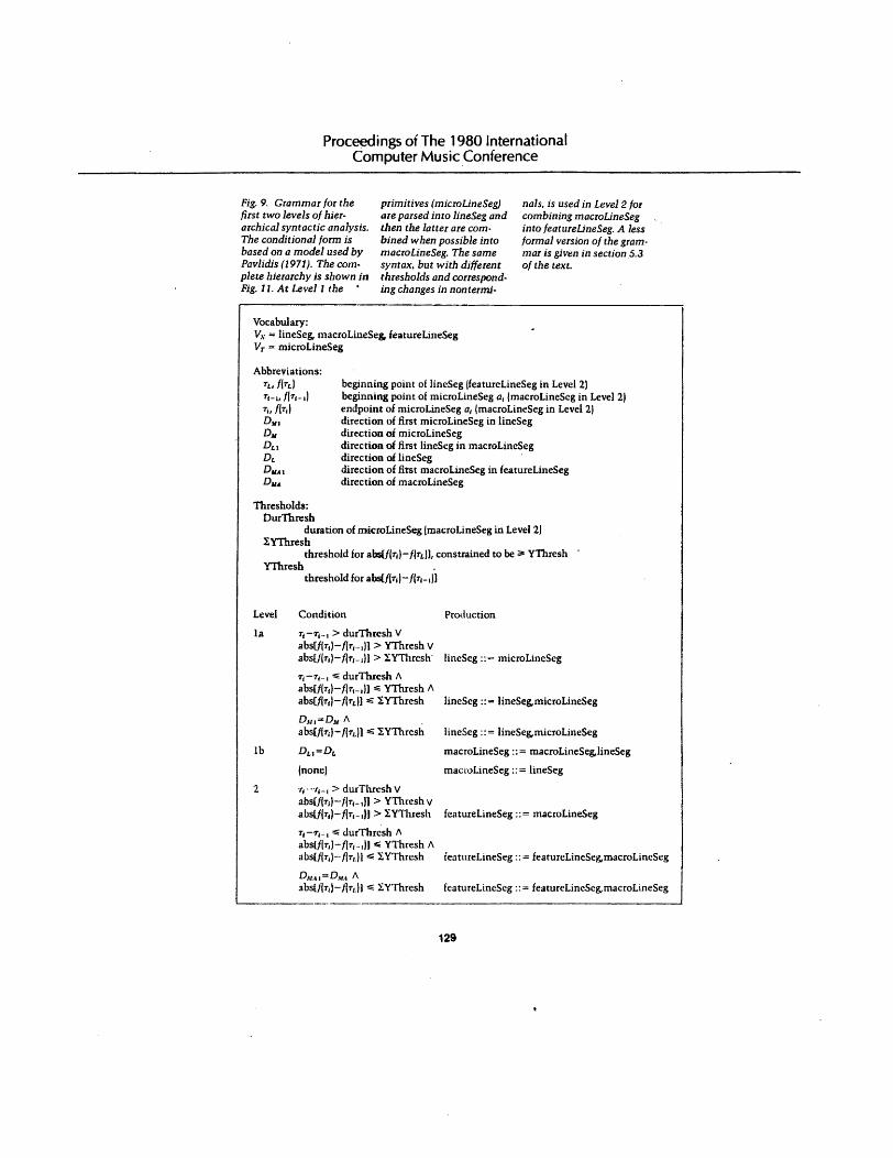
Fig. 9. Grammar for the first two levels of hier­archical syntactic analysis. The conditional form is based on a model used by Pavlidis (1971). The com­plete hierarchy is shown in Fig. 11. At Level 1 the •

Vocabulary:

primitives (microlineSeg) are parsed into lineSeg and then the latter are com­bined when possible into macrolineSeg. The same syntax, but with different thresholds and correspond­ing changes in nontermi-

Vv = lineSeg, macroLineSe& featureLineSeg VT= microLineSeg

Abbreviations:

nals, is used in Level 2 for combining macrolineSeg into featurelineSeg. A less formal version of the gram­mar is given in section S.3 of the text.

TL, f{Td T1-i. flT1-1I T1, f1T1I DJ11

beginning point of lincSeg (featureLineSeg in Level 2) beginning point of microLineSeg a1 {macroLineScg in Level 21 endpoint of microLineSeg a1 (macroLineSeg in Level 21 direction of first microLineSeg in lineSeg

D11 Du DL D1u.1 D,,,,.

di1ectioo of microLineSeg direction of first lineSeg in macroLineSeg direction of lineSeg direction of fitst macroLineSeg in featureLineSeg direction of macroLineSeg

Thresholds: Our Thresh

duration of microLineSeg (macroLineSeg in Level 21 IYThresb

threshold for abs(f{Ti)-flTLJ], constrained to be ;;io YThresh YThresh .

threshold for absCflT1l-f1T1-1l1

Level Condition Production

la. T1-T1-1 > durThresh V absCflT1)-f1T1-11l > YThresh V

lb

abs[/{T1)-f1T1- 11l > IYThresh· lineSeg ::= microLineSeg

T1-T1-1 '"'durThresh A abs[f(T,)-flT1-1l1,.. YThresh A absUITil-flTL)] E; IYThresh lineSeg ::= lineSeg,microLineSeg

D.m=DM A abs[f(T1)-f(TLIJ E; IYThrcsh lineSeg ::= lineSeg,microLineSeg

macroLineSeg ::= macroLineSeg,lineSeg

macroLineSeg ::= lineSeg

2 r1 ···t1- 1 > du1Tlucsh V abs[f(T1)-f{T1-1Jl > YThresh v abslflT1)-f{T1-1U > IYTluesh featureLineSeg ::= macroLineSeg

T1-T1 - 1 ,.;; durThrcsh /\ abs(f(T,)-f(T1-1ll ~ YThresh A abs[flT1)-f(T1.)I.;; IYThrcsh featureLineSeg ::= featurcLincSeg,macroLincSeg

DAt,u=DJu A abs(/lT1)-/lT1.ll'"' IYThresh featureLincScg ::= featureLincScg,macroLineSeg

129

Proceedings of The 1980 International Computer Music Conference

between the initial silence and the steady-state is classified as attack; everything after the steady­state is decay. If no steady-state is found, then as many successive up featureLineSeg as possible are grouped together following the initial silence to form the attack, and the remaining featureLineSeg are assigned to the decay. It should be emphasized that the attack-steady-state-decay terminology is used merely for convenience in labeling part of the syntactic analysis, with no semantic implica­tions, at least at this stage.

5.4 Analysis of Amplitude Functions

Figure 10 shows an analysis of the waveform of Fig. 1 at every stage of the hierarchical analysis. None of these plots represents the ultimate form of the output from this method of analysis; further processing is envisioned, as will be discussed. How· ever, by adjusting the thresholds properly, data reduction at, say, the lineSeg level IFig. lO[a]) can be achieved which will probably be useful in a wide variety of cases.

The model for the analysis of an amplitude wave· form assumes:that the note will consist of the pans discussed above. This attack-steady-state-decay model has been widely used in commercial analog synthesizers. The fact that it appears here is merely coincidental. The class of waveforms for which this software has been optimized is restricted to wave· forms derived from a limited set of test tones lasting, typically, one-quarter of a second or longer.

Ultimately these programs will be used to ana· lyze two or thrt:e such notes playe.d in succession, either separated by silence or connected in some way jlegato, portato, etc). In fact, the software has already been implemented to handle such groups of notes. Briefly, the output of a given channel of the phase vocoder is first compared with an amplitude threshold. Notes are initially defined within the en· tire function as being separated by periods of silence. The hierarchical analysis is then performed on a note-by-note basis. Each period of silence is as· signed to the note immediately following. The entire function is thus represented as a linked list

of notes followed by an optional silence. Each note, in turn, includes an optional initial silence, attack, decay, and optional steady-state. Within each note, the line segments at a given hierarchical level are represented as a linked list of records. A line seg· ment at one hierarchical level also has pointers to one or more line segments at the next lower hier­archical level which the line segment at the higher level encompasses.

5.5 Analysis of Frequency Functions

This preliminary division of a function into notes incorporates the notion of planning originally for­mulated by Minsky I 1963) but used here as developed by Kelly (1971). Planning is further ap· plied to the analysis of the frequency functions produced by the phase vocoder, which is especially problematical at low amplitudes where the fre­quency traces varies widely IFig. l[b]). There is also the problem of phase wraparound, which occasion· ally produces characteristic spikes in the frequency trace. Before the frequency traces are submitted to syntactic analysis, these spikes are removed from the regions of the frequency trace bounded by the attack-steady-state-decay parts of the notes in the amplitude function. These same portions of the frequency trace are then analyzed syntactically using the grammar already given in Fig. 9. Details of the assignment of featureLineSeg to the parts of a note vary slightly for the frequency functions but the basic approach is the same. Fig. 11 shows the results of syntactic, hierarchical analysis of the fre· quency trace belonging to the same harmonic as the tone shown in Fig. 10. Obviously the thresholds are different for amplitude and frequency functions. Given the diverging abilities of the ear to discrimi· nate frequency and amplitude, it would not be surprising if the higher-level analysis of frequency functions could eventually be simplified or modi· fied somewhat.

An entire musical phrase is thus represented as a linked list of phase vocoder channel outputs. Each channel consists of an amplitude and frequency function. Each function in turn points to a linked .

130

Fig. 10. Syntactic bier· archical analysis of the amplitude waveform shown in Fig. 1. (a) line· Seg, resulting from analy­sis of microlineSeg, with DurThresh = 0.01 sec, ¥Thresh= 0.01, and

0

0

0

0

0

Proceedings of The 1980 International Computer Music Conference

IYThresh 0.1. (b) line· Seg of the same direction have been combined into macrolineSeg. (c) fea­turelineSeg, with Dur· Thresh = 0.1 sec, YTl1resh = 0.2, and IYThresh = 0.4. (d) Analysis of feature·

0.25 Time

0.25 Time

0.25

Time

0.25 Time

LineSeg into parts of a note. The "direction" of the straight line from t ""' 0.1 sec tot"" 0.175 sec in (c) is analyzed as being di­agonal (pointing down­ward) and therefore is not classified as belonging to a

0.5

0.5

0.5

0.5

131

steady-state. There are 65 . line segments in the ap·

proximation of (a), 19 line segments in (b), and 7 in (c).

Fig. JI. ~yntc1dic hier­archicul analysis of the frec1uency function of Fig. 1(b). The vertical line ex­tending to the x-ax.is un the right-hand side is an artifact of tbe display rou­tine used for plotting; com­pare this with Fig. 1(b). (a) lineSeg. resulting from analrsis with DurThresh = 0.01 sec. YThresh = 2,

(al

1500

1250

0

(bl

;:... 1500 u c:: QJ ;:J O"' ~ 1250 (.I.,

0

(cl

;:... 1500 u c:: QJ ;:J O"' ~ 1250 (.I.,

0

(d) 1500

;:... u c:: QJ ;:J O' ~

(.I., 1250

0

Proceedings of The 1980 International Computer Music Conference

and ~YThresh = 5 (YThresh and ~YThresh in Hertz). (b) lineSeg of the same direction have been combined into macroLine­Seg. (c) featureLfneSeg, with DurThresh = 0.1 sec, YThresh = 10, and I Y­Thresh = 30. (d) Analysis of featureLineSeg into parts of a note. The "de­cay" slopes slightly down-

0.25 Time

0.25 Time

0.25 Time

0.25 Time

ward because it is con­strained to end at a point which occurs at the same time as the final point of the note found in the am­plitude function. As stated in the text, however. use of the terms attack. steady­state, and decay is merely for the sake of conve­nience. The top-down parse allows such pre-

132

liminary analysis /U be ,. refined consideral>Jy before

arrival at a final set of breakpoints for such a function. There are 80 line segments in the approx­imation of (a), 46 line segments in (b), and 14 in (c).

0.5

0.5

0.5

0.5

Proceedings of The 1980 International Computer Music Conference

Fig. 12. Overview of the data structure used in the hierarchical syntactic analysis. Curly brackets are used to delineate a

two-way linked list of rec­ords; the arrangement of pointers between hier­archical levels indicates one of many possible con-

figurations. Names of the hierarchical levels are en· closed in parentheses.

musical phrase J L {amp channel 1 - amp channel 2 - ... - amp channel n} (phrase)

! t !t ! t {freq channel I - freq channel 2 - ... - freq channel n}

{phase vocoder channel)·

{ampNote1 - ampNote2 - ••• - ampNote,. - final silence} (notel

~ . t +

{freqNote, - freqNot~ - ... freqNote,. - final silence}

{ sHence, attack, steady-state, decay} [ {silence, ~ttack, stead:sute, decay) .. ~ ~pa~ of not el

! ! + !~· ' ~ ' {fls, +-+ fls1 - - fls,. - fls11 +-> fls,} (fcatureLineSeg)

1 t r~1 {ma,+-+ ma~,... - ma..i - mar+-+ ma.} (macroLineSeg)

l~ .-J! l fli, ,... li2 .-. +-> Ii., - lii, -I~.} (lineSeg)

!~ t .Jl {mi1 +-+mi~,... - mia - mip - mi.y} (microLineSeg)

list of notes which are individually analyzed in terms of the grammar presented here. The complete structure is summarized in Fig. 12.

5.6 Refinement: A Top-Down Parse

This "bottom-up" parse. is only the beginning of a projected system, shown in Fig. l3. Once the at·

133

tack, steady-state, and decay portions of the amplitude function have been found, they can be utilized in terms of planning as a guide for a "top· down" directed search for features to be included in the final set of breakpoints. The output would thus no longer be grouped according to attack, steady· state, or decay. Rather, it would consist of the br;::akpoints found and confirmed b)(. the top-down analysis.

Proceedings of The 1980 International Computer Music Conference

Prcprm;essmg of current function {Planning): ampiitud,•: silence threshold for determining "notes"

fm.1ucncy: remove rhase wraparound artifacts

amplitude fun.:tiun: syntactic an.1lysis: bottom·up parse

1st hierarchical level: remove small features 2nd hierarchical lcvd: n:mov.: larger fc~tures

.lrll hicr.m:hical levd: assign larger fc?tures to parts of notl' refine syntacm: analysis: top·down pa~

frequency function: tusc amplitude function as gunlcl syntactic analysis: bottom-up parse

1st hierarchical level: rcmove small features 2nd hierarchical levd: remove largcr ft:atures •

3rd hierarchical lcvd: assign larger features to parts of note refine syntactic an.1lysis: mp·duwn parse

134

Fig. 13. Overview of the proposed analysis system in its final form, modeled after a system used in paL· tern recognition (Fu 1974, p. 5; Rosenfeld 1969, p. 105).

y

refine all functions for current note

confirm and refine note/silence boundaries

N

y

Proceedings of The 1980 International Computer Music Conference

Fig. 14. In this figure, the endpoints of an approx­imating line segment are not constrained to be points of the original data. The solid lines represent

100

75

some line-segment approx­imation to a function (dot­ted line). The parser has decided that an additional breakpoint is to be in· serted near the bottom of

' I

I I ,

I

-···· , .. ·· ... ' ', ... /·~

.... \'

• • I .. ··· \ : ,' \ :• : I • I\ ·• •I .• , : :,

~·\: r .. , \ I!

:,1 ., 1:

l \ '' l

so

\l 25

0 250 500

Consider the blips in the attack portion of the amplitude waveform analyzed in Fig. 10. A blip can be represented as a characteristic succession of line segments !e.g., up-down-up, or up-horizontal-down· up! at the lineSeg level. Such a pattern can easily be found using syntactic analysis. The juncture of "at­tack" and "steady-state" can be refined similarly, for example, by "tracking" to extend each part as far as possible (Shirai 1973) oi; to include an initial "overshoot" at the beginning of the steady-state.

After each function is refined in this manner, the entire family of functions can be scanned to con-

135

the "valley," as indicated by the dashed lines. But in order to do so, the original endpoints for the solid line must be recalculated. This additional computational

750

overhead is reduced in the current implementation by the requirement of Eq. (3).

firm the acceptability of various features for each note (cf. Fig. 13). For example, a flag can be set to retain a blip in an amplitude function only if the blip occurs at the same place in, say, more than two harmoriics. The initial segmentation of the phase vocoder channel outputs into notes can likewise be confirmed by comparing all of the functions. It · might happen that a spurious "silence" detected in some amplitude function would result in an er· roneous initial division of one note into two. Such an error can be corrected at this stage.

This also provides, at long last, the justification

Proceedings ofThe 1980 International Computer Music Conference

for requiring that all breakpoints in the approxima­tion be identical to points of the original waveform jEq. [3]). If the approximations at the various hier­archical levels could include other points, then a large amount of recomputation would be necessary every time a breakpoint were modified !Fig. 14). In other words, it seems reasonable at this stage to re­quire that the analysis retain some of the low-level information, in the form of the original data points, at higher levels of the pa'rse. This requirement may have to be modified later, however, if it turns out that a significant reduction in· the final number of segments can be achieved by doing so.

Other methods from pattern recognition will probably prove useful in this work. Perhaps stochastic syntax analysis {Fu 1974) in the bottom­up parse would reduce the amount of refining to be done later. The Hough transform {Duda and Hart 1973; Iannino and Shapiro 1978) might also prove useful for deciding, for example, that four points defining two separated line segments a, and ai+k, k > l, were actually colinear and that the entire function between them could be represented as a single line.

6. Summary and Conclusion

Various algorithms from the literature on approx­imation theory and pattern recognition have been shown to be useful for approximating waveforms in digital sound synthesis. A syntactic analysis scheme has also been presented which will ul­timately be extended to a generalized parse1 for amplitude and frequency functions.

This work represents.,one aspect of the growing application of artificial intelligence {AI) techniques to musical problems. The syntax and data structure here could easily be extended to a system for in­strument recognition similar to the speech-recogni· tion system Hearsay (Erman and Lesser 1975; Erman 1976). A scheme for automatic transcription of music could also be derived which in turn could be used to drive a music-analysis system such as that developed by Tenney ( 1978). The syntactic analysis presented here will also be useful for ap­proximating other time-varying waveforms in a wide variety of musical applications.

7. Acknowledgments

Dexter Morrill {Colgate University) provided t:he trumpet tone used as an example in this paper. In addition to assisting at every stage of this work, James A. Moorer {CCRMAJ contributed consider­ably to the design and implementation of the syntactic analysis. l would also like to express my appreciation to my teachers and colleagues for their time, patience, and many helpful suggestions: John Chowning, John Grey, and Julius Smith {CCRMAI; Barry Soroka {Stanford Al Project); and Curtis Roads.

References

Attneave, F. 1954. "Some Informational Aspects of Visual Perception." Psychological Review 61 : 183-193.

Beauchamp, James W. 1969. "A Computer System for nme-Variant Harmonic Analysis and Synthesis of Mu­sical Tones." In Music By Computer, ed. Heinz von Foerster and James Beauchamp. New York: John Wiley and Son.

Cox, M. G. 1971. "An Algorithm for Approximating Con­vex Functions by Means of First-Degree Splines." Computer foumal 14: 272-275.

Davis, Philip J., 1963. Interpolation and Approximation. New York: Blaisdell.

Davis, Larry S. 1977. "Shape Matching Using Relaxation Techniques." Proc. 1977 IEEE Conf. on Pattern Recogni­tion and Image Processi11g. Rensselaer, New York, pp. 191-197.

Davis, Larry S., and Rosenfeld, Azriel. 1978. "Hierarchical Relaxation for Waveform Parsing." In Computer Vision Systems, ed. Allen R. Hanson and Edward M. Riseman. New York: Academic Press, pp. 101-109.

Duda, Richard 0., and Hart; Peter E. 1973. Pattern Classi­fication and Scene Analysis. New York: John Wiley and Son.

Dudani, Sahibsingh, and Luk, Anthony L. 1977. "Locating Straight-Line Edge Segments on Outdoor Scenes." Proc. 1977 IEEE Con{. on Pattern Recognition and Image Processing. Rensselaer, New York, pp. 367-377.

Erman, Lee D. 1976. "Overview of the Hearsay Speech Understanding Research." SJGART Newsletter 56: 9-16.

Erman, Lee D., and LesS'er, Victor R. 1975. "A Multi-Level Organization for Problem Solving using Many, Diverse, Cooperating Sources of Knowledge." In Advance Pa-

136

Proceedings of The 1980 International Computer Music Conference

pers. Fourth International Conference on AI, Tbilisi, USSR, pp. 483-490.

Fu, K. S. 1974. Syntactic Methods in Pattern Recognition. New York: Academic Press.

Grey, fohn M. 1975. "An Exploration of Musical Timbre.'' Ph.D. thesis, Stanford University. Distributed as De­panment of Music Report No. Stan-M-2.

Iannino, Anthoily, and Shapiro, Stephen D. 1978. "A Sur· vey of the Hough Transform and its Extensions for Curve Detection." In Proc. IEEE Conf. Pattern Recogni­tion and Image Processing. Chicago, 1978, pp. 32-38.

Kelly, M. D. 1971. "Edge Detection in Pictures by Com­puter Using Planning." Machine Intelligence 6: 397-409.

Knuth, D. E. 1968. "Semantics of Context-Free Lan­guages."/. Mathematical Systems Theory 2: 127-146.

Minsky, Marvin. 1963. "Steps tow;ird Artificial Intel· ligence." In Computers and Thought, ed. Edward Feigenbaum and Julian Feldman. New York: McGraw· · Hill, pp. 406-450.

Moorer, James A. 1973. "The Heterodyne Method of Analysis of Transient Waveforms." Artificial Intel­ligence Laboratory Memo AIM-208. Stanford: Stanford University.

Moorer, James A. 1976. "The Use of the Phase Vocoder in Computer Music Applications." foumal of the Audio Engi11eering Society 26( 112): 42-45.

Moorer, James A. 1977. "Signal Processing Aspects of Computer Music: A Survey." Proceedings of the IEEE 65{8): 1108-1137. .

Moorer, James A. 1980. Personal communication. Moorer, James A.; Grey, John M.; and Strawn, John. 1978.

"Lexicon of Analyzed Tones. Part3: The Trumpet." Computer Music foumal 2121: 23-J l.

Pavlidis, Theodosios. 1971. "Linguistic Analysis of Wave­forms." In Software Engineering, vol. 2, ed. Julius T. Tou. New York: Academic Press, pp. 203-225.

Pavlidis, Theodosios. 1973. "Waveform Segmentation through Functional Approximation." IEEE Tr.wsactions on Computers C-2217):689-697.

137

Pavlidis, Theodosios, and Horowitz, Steven L. 1974. "Seg­mentation of Plane Curves." IEEE Transactions on Computers C-23(8): 860-870.

Pavlidis, Theodosios, and Maika, A. P. 1974. "Uniform Piecewise Polynomial Approximation with Variable Joints." foumal of Approximation Theory 12:61-69.

Phillips, G. M. 19613. "Algorithms for Piecewise Straight Line Approximations." Computer fournal 11: 2 l l-212.

Portnoff. M. R. 1976. "Implementation of the Digital Phase Vocoder Using the Fast Fourier Transform.'' IEEE Transactions on Acoustics, Speech, and Signal Process­ing ASSP-24:243-248.

Risset, Jean-Claude, and Mathews, Max V. 1969. "Analy­sis of Musical-Instrument Tones." Physics Today 2212):23-30.

Rosenfeld, Azricl. 1969. Picture Processing by Computer. New York: Academic Press. .

Shirai, Yoshiaki. 1973. "A Context-Sensitive Line Finder for Recognition of Polyhedra." Artificial Intelligence 4(2):95-119.

Shirai, Yoshiaki. 1978. "Recognition of Real-World Ob­jects Using Edge Cue." In Computer Vision Systems, ed. Allen R. Hanson and Edward M. Riseman. New York: Academic Press, pp. 353-362.

Stone, Henry. 1961. "Approximation of Curves by Line Segments." Mathematics of Computation IS: 40-47.

Strong, William, and Clark, Melville. 1967. "Synthesis of Wind-Instrument Tones.'' fournal of the Acoustical So· ciety of America 41 ( l): 39-52.

Symons, M. 1968. "A New Self-organising Pattern Recog­nition System." Conference on Pattern Recognition. Teddington, pp. 11-20. ·

Tenney, James (with Polansky, Larry). 1978. Hierarchical Temporal Gestalt Perception in Music: A "Metric Space" Model. Toronto: York University.

Tou, Julius T., and Gonzales, Rafael C. 1974. Pattern Rec­ognition Principles. Reading, Massachusetts: Addison­Wesley.