Water Utility Direct Avoided Costs From Water Use Efficiency

PowerPoint Authors:Susan Coomer Galbreath, Ph.D., CPACharles W. Caldwell, D.B.A., CMAJon A. Booker, Ph.D., CPA, CIACynthia J. Rooney, Ph.D., CPA
Copyright © 2012 by The McGraw-Hill Companies, Inc. All rights reserved.
Standard Costs and VariancesChapter 10
10-2
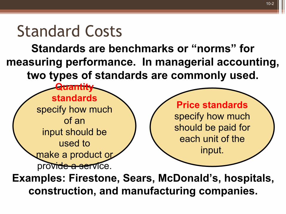
Standard CostsStandards are benchmarks or “norms” for
measuring performance. In managerial accounting,two types of standards are commonly used.
Quantity standards
specify how much of an
input should be used to
make a product orprovide a service.
Price standardsspecify how muchshould be paid for
each unit of theinput.
Examples: Firestone, Sears, McDonald’s, hospitals, construction, and manufacturing companies.

10-3
Standard Costs
DirectMaterial
Deviations from standards deemed significantare brought to the attention of management, apractice known as management by exception.
Type of Product Cost
Am
ount
DirectLabor
ManufacturingOverhead
Standard

10-4
Variance Analysis Cycle

10-5
Setting Standard Costs
Should we useideal standards that
require employees towork at 100 percent
peak efficiency?
Engineer Managerial Accountant
I recommend using practical standards that are currently attainable with reasonable
and efficient effort.

10-6
Setting Direct Materials Standards
Standard Priceper Unit
Summarized in a Bill of Materials.
Final, deliveredcost of materials,net of discounts.
Standard Quantityper Unit

10-7
Setting Direct Labor Standards
Use time and motion studies for
each labor operation.
Standard Hoursper Unit
Often a singlerate is used that reflectsthe mix of wages earned.
Standard Rateper Hour

10-8
Setting Variable Manufacturing Overhead Standards
The rate is the variable portion of the
predetermined overhead rate.
PriceStandard
The quantity is the activity in the
allocation base for predetermined overhead.
QuantityStandard

10-9
The Standard Cost Card
A standard cost card for one unit of product might look like this:

10-10
Using Standards in Flexible Budgets
Standard costs per unit for direct materials, direct labor, and variable manufacturing overhead can be used to compute activity and spending variances.
Spending variances become more useful by breaking them down into
quantity and price variances.

10-11
A General Model for Variance Analysis
Variance Analysis
Price Variance
Difference betweenactual price and standard price
Quantity Variance
Difference betweenactual quantity andstandard quantity

10-12
Quantity and Price Standards
Quantity and price standards are determined separately for two reasons:
❶ The purchasing manager is responsible for raw material purchase prices and the production manager is responsible for the quantity of raw material used.
❷ The buying and using activities occur at different times. Raw material purchases may be held in inventory for a period of time before being used in production.

10-13
Variance Analysis
Materials price varianceLabor rate varianceVOH rate variance
Materials quantity varianceLabor efficiency varianceVOH efficiency variance
A General Model for Variance Analysis
Quantity Variance Price Variance

10-14
A General Model for Variance Analysis
Quantity Variance(2) – (1)
Price Variance(3) – (2)
(1)Standard Quantity
Allowed for Actual Output,at Standard Price
(SQ × SP)
(2)Actual Quantity
of Input,at Standard Price
(AQ × SP)
(3)Actual Quantity
of Input,at Actual Price
(AQ × AP)
Spending Variance(3) – (1)

10-15
A General Model for Variance AnalysisActual quantity is the amount of direct materials, direct
labor, and variable manufacturing overhead actually used.
Quantity Variance(2) – (1)
Price Variance(3) – (2)
(1)Standard Quantity
Allowed for Actual Output,at Standard Price
(SQ × SP)
(2)Actual Quantity
of Input,at Standard Price
(AQ × SP)
(3)Actual Quantity
of Input,at Actual Price
(AQ × AP)
Spending Variance(3) – (1)

10-16
A General Model for Variance Analysis Standard quantity is the standard quantity allowed
for the actual output of the period.
Quantity Variance(2) – (1)
Price Variance(3) – (2)
(1)Standard Quantity
Allowed for Actual Output,at Standard Price
(SQ × SP)
(2)Actual Quantity
of Input,at Standard Price
(AQ × SP)
(3)Actual Quantity
of Input,at Actual Price
(AQ × AP)
Spending Variance(3) – (1)

10-17
A General Model for Variance Analysis Actual price is the amount actually
paid for the input used.
Quantity Variance(2) – (1)
Price Variance(3) – (2)
(1)Standard Quantity
Allowed for Actual Output,at Standard Price
(SQ × SP)
(2)Actual Quantity
of Input,at Standard Price
(AQ × SP)
(3)Actual Quantity
of Input,at Actual Price
(AQ × AP)
Spending Variance(3) – (1)

10-18
A General Model for Variance Analysis
Quantity Variance(2) – (1)
Price Variance(3) – (2)
(1)Standard Quantity
Allowed for Actual Output,at Standard Price
(SQ × SP)
(2)Actual Quantity
of Input,at Standard Price
(AQ × SP)
(3)Actual Quantity
of Input,at Actual Price
(AQ × AP)
Spending Variance(3) – (1)
Standard price is the amount that shouldhave been paid for the input used.

10-19
Learning Objective 1
Compute the direct materials quantity and
price variances and explain their significance.

10-20
Glacier Peak Outfitters has the following direct materials standard for the fiberfill in its mountain
parka.
0.1 kg. of fiberfill per parka at $5.00 per kg.
Last month 210 kgs. of fiberfill were purchased and used to make 2,000 parkas. The materials cost a
total of $1,029.
Materials Variances – An Example

10-21
200 kgs. 210 kgs. 210 kgs. × × × $5.00 per kg. $5.00 per kg. $4.90 per kg.
= $1,000 = $1,050 = $1,029
Quantity variance$50 unfavorable
Price variance$21 favorable
Materials Variances Summary
Standard Quantity Actual Quantity Actual Quantity × × × Standard Price Standard Price Actual Price

10-22
Materials Variances Summary
200 kgs. 210 kgs. 210 kgs. × × × $5.00 per kg. $5.00 per kg. $4.90 per kg.
= $1,000 = $1,050 = $1,029
Quantity variance$50 unfavorable
Price variance$21 favorable
Standard Quantity Actual Quantity Actual Quantity × × × Standard Price Standard Price Actual Price
0.1 kg per parka × 2,000 parkas = 200 kgs

10-23
Materials Variances Summary
200 kgs. 210 kgs. 210 kgs. × × × $5.00 per kg. $5.00 per kg. $4.90 per kg.
= $1,000 = $1,050 = $1,029
Quantity variance$50 unfavorable
Price variance$21 favorable
Standard Quantity Actual Quantity Actual Quantity × × × Standard Price Standard Price Actual Price
$1,029 ÷ 210 kgs = $4.90 per kg

10-24
Materials Variances:Using the Factored EquationsMaterials quantity variance
MQV = (AQ × SP) – (SQ × SP) = SP(AQ – SQ)
= $5.00/kg (210 kgs – (0.1 kg/parka × 2,000 parkas)) = $5.00/kg (210 kgs – 200 kgs) = $5.00/kg (10 kgs) = $50 U
Materials price varianceMPV = (AQ × AP) – (AQ × SP) = AQ(AP – SP) = 210 kgs ($4.90/kg – $5.00/kg) = 210 kgs (– $0.10/kg) = $21 F
10-25
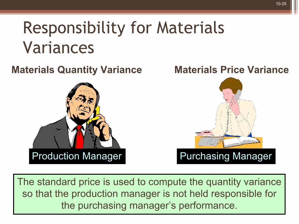
Materials Price VarianceMaterials Quantity Variance
Production Manager Purchasing Manager
The standard price is used to compute the quantity varianceso that the production manager is not held responsible for
the purchasing manager’s performance.
Responsibility for Materials Variances

10-26
I am not responsible for this unfavorable materials
quantity variance. You purchased cheapmaterial, so my peoplehad to use more of it.
Your poor scheduling sometimes requires me to rush order materials at a
higher price, causing unfavorable price variances.
Responsibility for Materials Variances
Production Manager Purchasing Manager

10-27
Hanson Inc. has the following direct materials standard to manufacture one Zippy:
1.5 pounds per Zippy at $4.00 per pound
Last week, 1,700 pounds of materials were purchased and used to make 1,000 Zippies. The
materials cost a total of $6,630.
ZippyQuick Check ✓

10-28
How many pounds of materials should Hanson have used to make 1,000 Zippies?a. 1,700 pounds.b. 1,500 pounds.c. 1,200 pounds.d. 1,000 pounds.
ZippyQuick Check ✓

10-29
ZippyQuick Check ✓
How many pounds of materials should Hanson have used to make 1,000 Zippies?a. 1,700 pounds.b. 1,500 pounds.c. 1,200 pounds.d. 1,000 pounds. The standard quantity is:
1,000 × 1.5 pounds per Zippy.

10-30
Hanson’s materials quantity variance (MQV)for the week was:a. $170 unfavorable.b. $170 favorable.c. $800 unfavorable.d. $800 favorable.
ZippyQuick Check ✓

10-31
Hanson’s materials quantity variance (MQV)for the week was:a. $170 unfavorable.b. $170 favorable.c. $800 unfavorable.d. $800 favorable.
MQV = SP(AQ - SQ) MQV = $4.00(1,700 lbs - 1,500 lbs) MQV = $800 unfavorable
ZippyQuick Check ✓

10-32
Hanson’s materials price variance (MPV)for the week was:a. $170 unfavorable.b. $170 favorable.c. $800 unfavorable.d. $800 favorable.
ZippyQuick Check ✓

10-33
Hanson’s materials price variance (MPV)for the week was:a. $170 unfavorable.b. $170 favorable.c. $800 unfavorable.d. $800 favorable. MPV = AQ(AP - SP)
MPV = 1,700 lbs. × ($3.90 - 4.00) MPV = $170 Favorable
ZippyQuick Check ✓

10-34
1,500 lbs. 1,700 lbs. 1,700 lbs. × × × $4.00 per lb. $4.00 per lb. $3.90 per lb.
= $6,000 = $ 6,800 = $6,630
Quantity variance$800 unfavorable
Price variance$170 favorable
ZippyQuick Check ✓
Standard Quantity Actual Quantity Actual Quantity × × × Standard Price Standard Price Actual Price

10-35
1,500 lbs. 1,700 lbs. 1,700 lbs. × × × $4.00 per lb. $4.00 per lb. $3.90 per lb.
= $6,000 = $ 6,800 = $6,630
Quantity variance$800 unfavorable
Price variance$170 favorable
ZippyQuick Check ✓
Standard Quantity Actual Quantity Actual Quantity × × × Standard Price Standard Price Actual Price
Recall that the standard quantity for 1,000 Zippiesis 1,000 × 1.5 pounds per Zippy = 1,500 pounds.

10-36
Learning Objective 2
Compute the direct labor efficiency and rate
variances and explaintheir significance.

10-37
Glacier Peak Outfitters has the following direct labor standard for its mountain parka.
1.2 standard hours per parka at $10.00 per hour
Last month, employees actually worked 2,500 hours at a total labor cost of $26,250 to make
2,000 parkas.
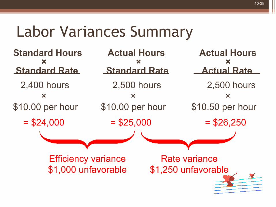
Labor Variances – An Example
10-38
Efficiency variance$1,000 unfavorable
Rate variance$1,250 unfavorable
Standard Hours Actual Hours Actual Hours × × × Standard Rate Standard Rate Actual Rate
Labor Variances Summary
2,400 hours 2,500 hours 2,500 hours × × ×$10.00 per hour $10.00 per hour $10.50 per hour
= $24,000 = $25,000 = $26,250

10-39
Labor Variances Summary
Efficiency variance$1,000 unfavorable
Rate variance$1,250 unfavorable
Standard Hours Actual Hours Actual Hours × × × Standard Rate Standard Rate Actual Rate 2,400 hours 2,500 hours 2,500 hours × × ×$10.00 per hour $10.00 per hour $10.50 per hour
= $24,000 = $25,000 = $26,250
1.2 hours per parka × 2,000 parkas = 2,400 hours

10-40
Labor Variances Summary
Efficiency variance$1,000 unfavorable
Rate variance$1,250 unfavorable
Standard Hours Actual Hours Actual Hours × × × Standard Rate Standard Rate Actual Rate 2,400 hours 2,500 hours 2,500 hours × × ×$10.00 per hour $10.00 per hour $10.50 per hour
= $24,000 = $25,000 = $26,250
$26,250 ÷ 2,500 hours = $10.50 per hour

10-41
Labor Variances: Using the Factored EquationsLabor efficiency variance
LEV = (AH × SR) – (SH × SR) = SR (AH – SH) = $10.00 per hour (2,500 hours – 2,400 hours) = $10.00 per hour (100 hours)
= $1,000 unfavorableLabor rate variance
LRV = (AH × AR) – (AH × SR) = AH (AR – SR) = 2,500 hours ($10.50 per hour – $10.00 per hour) = 2,500 hours ($0.50 per hour) = $1,250 unfavorable

10-42
Responsibility for Labor Variances
Production Manager
Production managers areusually held accountable
for labor variancesbecause they can
influence the:
Mix of skill levelsassigned to work tasks.
Level of employee motivation.
Quality of production supervision.
Quality of training provided to employees.

10-43
I am not responsible for the unfavorable labor
efficiency variance! You purchased cheap
material, so it took moretime to process it.
I think it took more time to process the
materials because the Maintenance
Department has poorly maintained your
equipment.
Responsibility for Labor Variances
10-44
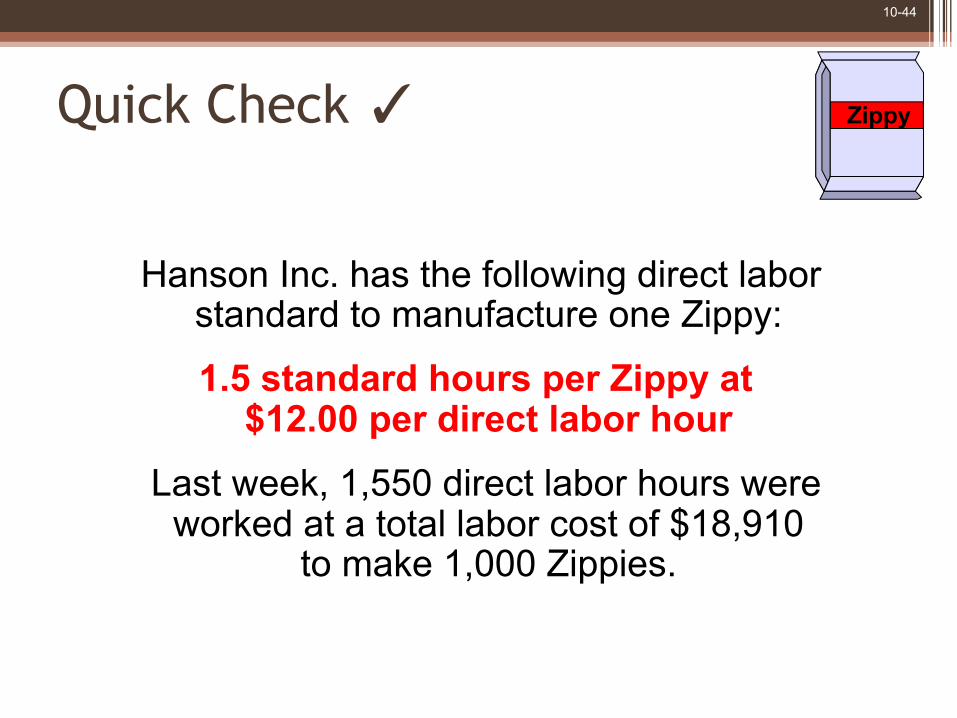
Hanson Inc. has the following direct laborstandard to manufacture one Zippy:
1.5 standard hours per Zippy at$12.00 per direct labor hour
Last week, 1,550 direct labor hours wereworked at a total labor cost of $18,910
to make 1,000 Zippies.
ZippyQuick Check ✓

10-45
Hanson’s labor efficiency variance (LEV)for the week was:a. $590 unfavorable.b. $590 favorable.c. $600 unfavorable.d. $600 favorable.
ZippyQuick Check ✓
10-46
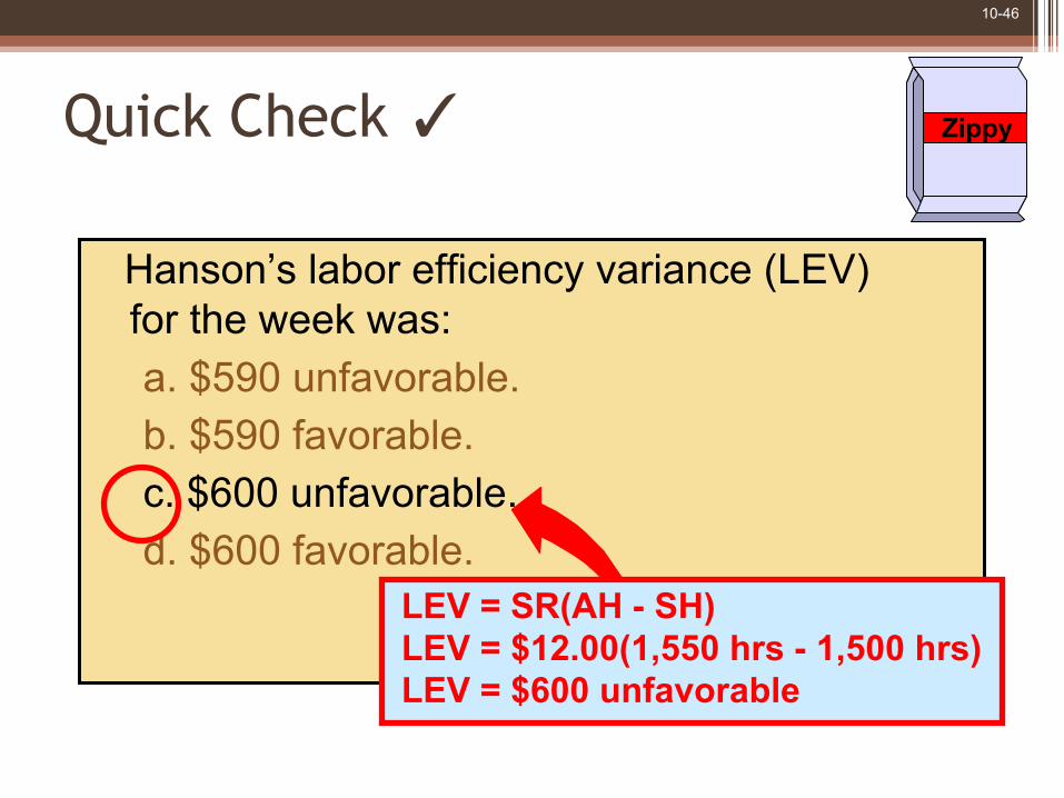
Hanson’s labor efficiency variance (LEV)for the week was:a. $590 unfavorable.b. $590 favorable.c. $600 unfavorable.d. $600 favorable.
LEV = SR(AH - SH) LEV = $12.00(1,550 hrs - 1,500 hrs) LEV = $600 unfavorable
ZippyQuick Check ✓

10-47
Hanson’s labor rate variance (LRV) for the week was:a. $310 unfavorable.b. $310 favorable.c. $300 unfavorable.d. $300 favorable.
ZippyQuick Check ✓

10-48
Hanson’s labor rate variance (LRV) for the week was:a. $310 unfavorable.b. $310 favorable.c. $300 unfavorable.d. $300 favorable.
LRV = AH(AR - SR) LRV = 1,550 hrs($12.20 - $12.00) LRV = $310 unfavorable
ZippyQuick Check ✓

10-49
Efficiency variance$600 unfavorable
Rate variance$310 unfavorable
1,500 hours 1,550 hours 1,550 hours × × × $12.00 per hour $12.00 per hour $12.20 per hour
= $18,000 = $18,600 = $18,910
ZippyQuick Check ✓
Standard Hours Actual Hours Actual Hours × × × Standard Rate Standard Rate Actual Rate

10-50
Learning Objective 3
Compute the variable manufacturing overhead
efficiency and rate variances and explain
their significance.

10-51
Glacier Peak Outfitters has the following direct variable manufacturing overhead labor standard for
its mountain parka.
1.2 standard hours per parka at $4.00 per hour Last month, employees actually worked 2,500
hours to make 2,000 parkas. Actual variable manufacturing overhead for the month was
$10,500.
Variable Manufacturing Overhead Variances – An Example

10-52
2,400 hours 2,500 hours 2,500 hours × × × $4.00 per hour $4.00 per hour $4.20 per hour
= $9,600 = $10,000 = $10,500
Efficiency variance$400 unfavorable
Rate variance$500 unfavorable
Variable Manufacturing Overhead Variances Summary
Standard Hours Actual Hours Actual Hours × × × Standard Rate Standard Rate Actual Rate

10-53
Variable Manufacturing Overhead Variances Summary
2,400 hours 2,500 hours 2,500 hours × × × $4.00 per hour $4.00 per hour $4.20 per hour
= $9,600 = $10,000 = $10,500
Efficiency variance$400 unfavorable
Rate variance$500 unfavorable
Standard Hours Actual Hours Actual Hours × × × Standard Rate Standard Rate Actual Rate
1.2 hours per parka × 2,000 parkas = 2,400 hours

10-54
Variable Manufacturing Overhead Variances Summary
2,400 hours 2,500 hours 2,500 hours × × × $4.00 per hour $4.00 per hour $4.20 per hour
= $9,600 = $10,000 = $10,500
Efficiency variance$400 unfavorable
Rate variance$500 unfavorable
Standard Hours Actual Hours Actual Hours × × × Standard Rate Standard Rate Actual Rate
$10,500 ÷ 2,500 hours = $4.20 per hour

10-55
Variable Manufacturing Overhead Variances: Using Factored EquationsVariable manufacturing overhead efficiency variance
VMEV = (AH × SR) – (SH – SR) = SR (AH – SH)
= $4.00 per hour (2,500 hours – 2,400 hours) = $4.00 per hour (100 hours)
= $400 unfavorableVariable manufacturing overhead rate variance
VMRV = (AH × AR) – (AH – SR) = AH (AR – SR) = 2,500 hours ($4.20 per hour – $4.00 per hour) = 2,500 hours ($0.20 per hour) = $500 unfavorable

10-56
Hanson Inc. has the following variablemanufacturing overhead standard to
manufacture one Zippy:
1.5 standard hours per Zippy at$3.00 per direct labor hour
Last week, 1,550 hours were worked to make1,000 Zippies, and $5,115 was spent for
variable manufacturing overhead.
ZippyQuick Check ✓

10-57
Hanson’s efficiency variance (VMEV) for variable manufacturing overhead for the week was:a. $435 unfavorable.b. $435 favorable.c. $150 unfavorable.d. $150 favorable.
ZippyQuick Check ✓

10-58
Hanson’s efficiency variance (VMEV) for variable manufacturing overhead for the week was:a. $435 unfavorable.b. $435 favorable.c. $150 unfavorable.d. $150 favorable.
VMEV = SR(AH - SH) VMEV = $3.00(1,550 hrs - 1,500 hrs) VMEV = $150 unfavorable
1,000 units × 1.5 hrs per unit
ZippyQuick Check ✓
10-59
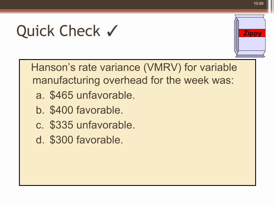
Hanson’s rate variance (VMRV) for variable manufacturing overhead for the week was:a. $465 unfavorable.b. $400 favorable.c. $335 unfavorable.d. $300 favorable.
ZippyQuick Check ✓

10-60
Hanson’s rate variance (VMRV) for variable manufacturing overhead for the week was:a. $465 unfavorable.b. $400 favorable.c. $335 unfavorable.d. $300 favorable.
VMRV = AH(AR - SR) VMRV = 1,550 hrs($3.30 - $3.00) VMRV = $465 unfavorable
ZippyQuick Check ✓

10-61
Efficiency variance$150 unfavorable
Rate variance$465 unfavorable
1,500 hours 1,550 hours 1,550 hours × × × $3.00 per hour $3.00 per hour $3.30 per hour
= $4,500 = $4,650 = $5,115
ZippyQuick Check ✓
Standard Hours Actual Hours Actual Hours × × × Standard Rate Standard Rate Actual Rate

10-62
Materials Variances―An Important Subtlety
The quantity variance is computed only on
the quantity used.The price variance is
computed on the entire quantity purchased.

10-63
Glacier Peak Outfitters has the following direct materials standard for the fiberfill in its mountain
parka.
0.1 kg. of fiberfill per parka at $5.00 per kg.
Last month 210 kgs. of fiberfill were purchased at a cost of $1,029. Glacier used 200 kgs. to make
2,000 parkas.
Materials Variances―An Important Subtlety

10-64
200 kgs. 200 kgs. × × $5.00 per kg. $5.00 per kg.
= $1,000 = $1,000
Quantity variance$0
Standard Quantity Actual Quantity × × Standard Price Standard Price
Materials Variances―An Important Subtlety

10-65
210 kgs. 210 kgs. × × $5.00 per kg. $4.90 per kg.
= $1,050 = $1,029
Price variance$21 favorable
Actual Quantity Actual Quantity × × Standard Price Actual Price
Materials Variances―An Important Subtlety

10-66
Variance Analysis and Management by Exception
How do I knowwhich variances to
investigate?
Larger variances, in dollar amount or as a percentage of the
standard, are investigated first.

10-67
A Statistical Control Chart
1 2 3 4 5 6 7 8 9Variance Measurements
Favorable Limit
Unfavorable Limit
• • • • •• • •
•
Warning signals for investigation
Desired Value

10-68
Advantages of Standard Costs
Management byexception
Advantages
Promotes economy and efficiency
Simplifiedbookkeeping
Enhances responsibility
accounting

10-69
PotentialProblems
Emphasis onnegative may
impact morale.
Emphasizing standardsmay exclude other
important objectives.
Favorablevariances may
be misinterpreted.
Continuous improvement maybe more important
than meeting standards.
Standard costreports may
not be timely.
Invalid assumptionsabout the relationship
between laborcost and output.
Potential Problems with Standard Costs

PowerPoint Authors:Susan Coomer Galbreath, Ph.D., CPACharles W. Caldwell, D.B.A., CMAJon A. Booker, Ph.D., CPA, CIACynthia J. Rooney, Ph.D., CPA
Copyright © 2012 by The McGraw-Hill Companies, Inc. All rights reserved.
Appendix 10A
Predetermined Overhead Rates and Overhead Analysis in a Standard Costing System

10-71
Learning Objective 4
(Appendix 10A)Compute and interpret
the fixed overhead volume and budget
variances.

10-72
Volumevariance
Fixed Overhead Volume VarianceFixed
OverheadApplied
ActualFixed
Overhead
BudgetedFixed
Overhead
Volumevariance
Fixedoverheadapplied to
work in process
Budgetedfixed
overhead= –

10-73
FPOHR = Fixed portion of the predetermined overhead rate DH = Denominator hours SH = Standard hours allowed for actual output
SH × FR DH × FR
Fixed Overhead Volume Variance
Volume variance FPOHR × (DH – SH)=
FixedOverheadApplied
ActualFixed
Overhead
BudgetedFixed
Overhead
Volumevariance

10-74
Budget variance
Fixed Overhead Budget Variance
Budgetvariance
Budgetedfixed
overhead
Actualfixed
overhead= –
FixedOverheadApplied
ActualFixed
Overhead
BudgetedFixed
Overhead

10-75
Computing Fixed Overhead Variances

10-76
Computing Fixed Overhead Variances

10-77
Predetermined Overhead Rates
Predetermined overhead rate
Estimated total manufacturing overhead costEstimated total amount of the allocation base=
Predetermined overhead rate
$360,00090,000 Machine-hours=
Predetermined overhead rate = $4.00 per machine-hour

10-78
Predetermined Overhead Rates
Variable component of thepredetermined overhead rate
$90,00090,000 Machine-hours=
Variable component of thepredetermined overhead rate = $1.00 per machine-hour
Fixed component of thepredetermined overhead rate
$270,00090,000 Machine-hours=
Fixed component of thepredetermined overhead rate = $3.00 per machine-hour

10-79
Applying Manufacturing Overhead
Overheadapplied
Predetermined overhead rate
Standard hours allowedfor the actual output= ×
Overheadapplied
$4.00 permachine-hour 84,000 machine-hours= ×
Overheadapplied $336,000=

10-80
Computing the Volume Variance
Volumevariance
Fixedoverheadapplied to
work in process
Budgetedfixed
overhead= –
Volumevariance = $18,000 Unfavorable
Volumevariance = $270,000 – $3.00 per
machine-hour( × $84,000machine-hours)

10-81
Computing the Volume Variance
FPOHR = Fixed portion of the predetermined overhead rate DH = Denominator hours SH = Standard hours allowed for actual output
Volume variance FPOHR × (DH – SH)=
Volumevariance
= $3.00 permachine-hour (× 90,000
mach-hours – 84,000mach-hours)
Volumevariance
= 18,000 Unfavorable

10-82
Computing the Budget Variance
Budgetvariance
Budgetedfixed
overhead
Actualfixed
overhead= –
Budgetvariance = $280,000 – $270,000
Budgetvariance = $10,000 Unfavorable

10-83
A Pictorial View of the VariancesFixed Overhead
Applied toWork in Process
ActualFixed
Overhead
BudgetedFixed
Overhead 280,000270,000252,000
Total variance, $28,000 unfavorable
Budget variance,$10,000 unfavorable
Volume variance,$18,000 unfavorable

10-84
Fixed Overhead Variances –A Graphic Approach
Let’s look at a graph showing fixed overhead
variances. We will use ColaCo’s
numbers from the previous example.

10-85
Graphic Analysis of FixedOverhead Variances
Machine-hours (000)
Budget$270,000
90
Denominatorhours
00
Fixed overhead applied at
$3.00 per standard hour

10-86
Graphic Analysis of FixedOverhead Variances
Actual$280,000
Machine-hours (000)
Budget$270,000
90
Denominatorhours
00
Fixed overhead applied at
$3.00 per standard hour
Budget Variance 10,000 U{

10-87
Applied$252,000
Machine-hours (000)
Budget$270,000
Graphic Analysis of Fixed Overhead Variances
908400
Standardhours
Fixed overhead applied at
$3.00 per standard hour
Denominatorhours
Budget Variance 10,000 U
Volume Variance 18,000 U
{{
Actual$280,000

10-88
Reconciling Overhead Variances and Underapplied or Overapplied OverheadIn a
standardcost
system:
Favorablevariances are equivalentto overapplied overhead.
The sum of the overhead variancesequals the under- or overapplied
overhead cost for the period.

10-89
Reconciling Overhead Variances and Underapplied or Overapplied Overhead

10-90
Computing the Variable Overhead Variances
Variable manufacturing overhead efficiency varianceVMEV = (AH × SR) – (SH × SR) = $88,000 – (84,000 hours × $1.00 per hour) = $4,000 unfavorable

10-91
Computing the Variable Overhead Variances
Variable manufacturing overhead rate varianceVMRV = (AH × AR) – (AH × SR) = $100,000 – (88,000 hours × $1.00 per hour) = $12,000 unfavorable

10-92
Computing the Sum of All Variances

PowerPoint Authors:Susan Coomer Galbreath, Ph.D., CPACharles W. Caldwell, D.B.A., CMAJon A. Booker, Ph.D., CPA, CIACynthia J. Rooney, Ph.D., CPA
Copyright © 2012 by The McGraw-Hill Companies, Inc. All rights reserved.
Journal Entries to Record Variances Appendix 10B
General Ledger Entries to Record Variances

10-94
Learning Objective 5
(Appendix 10B)Prepare journal entries
to record standardcosts and variances.

10-95
Glacier Peak Outfitters ― RevisitedWe will use information from the Glacier Peak Outfitters
example presented earlier in the chapter to illustrate journalentries for standard cost variances. Recall the following:
MaterialAQ × AP = $1,029AQ × SP = $1,050SQ × SP = $1,000MPV = $21 FMQV = $50 U
LaborAH × AR = $26,250AH × SR = $25,000SH × SR = $24,000LRV = $1,250 ULEV = $1,000 U
Now, let’s prepare the entries to recordthe labor and material variances.

10-96
Recording Materials Variances

10-97
Recording Labor Variances

10-98
Cost Flows in a Standard Cost System
Inventories are recorded at standard cost.Variances are recorded as follows:
• Favorable variances are credits, representing savings in production costs.
• Unfavorable variances are debits, representing excess production costs.
Standard cost variances are usually closed out to cost of goods sold.• Unfavorable variances increase cost of goods sold.• Favorable variances decrease cost of goods sold.
10-99
End of Chapter 10