STAGE: STAtistical modelling of Groundwater Extremes · STAGE: STAtistical modelling of Groundwater...

STAGE: STAtistical modelling of Groundwater Extremes

Ben Marchanta, Emma Eastoeb, Jenny Wadsworthb and John Bloomfieldc

July 29, 2016

a: British Geological Survey, Keyworth, NG12 5GG, UKb: Department of Mathematics and Statistics, Fylde College, Lancaster University, Lancaster, LA14YF, UKc: British Geological Survey, Maclean Building, Crowmarsh Gifford, Wallingford, Oxfordshire,OX10 8BB, UK

1 Summary

The primary aim of this feasibility study was to establish a sustainable collaborative relationshipbetween the British Geological Survey (BGS) and the Modelling and Inference Group at LancasterUniversity (LU) with particular focus on the study of extreme events in the earth sciences. Thiswas achieved through:

• A case study exploring extreme events in long-term (> 100 years) groundwater hydrographesfrom UK aquifers.

• Networking events designed to introduce BGS earth scientists to LU statisticians and toidentify research areas and funding opportunities for future collaborations.

Through the course of the case study, BGS researchers have been introduced to state-of-the-artextreme value statistics methodologies and have been provided with the knowledge and softwarerequired to replicate these analyses on other datasets. These methodologies are considerably moreflexible and generally applicable than those that currently appear in the hydrological literature.BGS continue to apply these methodologies to groundwater data within the NERC funded ’Analysisof historic drought and water scarcity in the UK’ and other internally funded projects concernedwith the drivers of groundwater levels. Once the methodologies have been tested on a wider rangeof datasets, BGS and LU envisage a joint publication assessing the suitability of extreme valuestatistics to predict the chacteristics of extreme groundwater events. BGS have included extreme

1

value techniques in a bid for funding from the NERC Knowledge Exchange Programme and in theIMPOWER (Impact for urban groundwater management program) proposal to a consortium ofrepresentatives of the water industry. BGS and LU will seek to collaborate in any future programsconcerned with the occurrence and risk of floods and droughts in the UK.

The networking activities identified several further topics that are suitable for future collab-orations including space-weather, volcanic eruptions, the retreat of glaciers, seismology and soilcontamination. These discussions have led to three MSc projects that are currently being con-ducted by LU students in collaboration with BGS scientists and further project proposals are beingdeveloped for the 2016-17 academic year. The project team see these MSc projects as an idealopportunity for the LU statisticians to make an initial assessment of the available data and thepotential for further work and applications for external funding. In each topic area, potentialsources for future funding have been identified. BGS and LU are producing a PhD proposal on thespatial prediction of soil properties for submission to the Soils Training and Research StudentshipsDoctoral Training Centre in October 2016.

2 Networking Activities

The following networking activities were conducted during the feasibility project:

2.1 Initial Meeting

A introductory project meeting at Lancaster University attended by Dr Emma Eastoe (LancasterUniversity Statistician), Dr Jenny Wadsworth (Lancaster University Statistician), Dr Ben Marchant(BGS Environmental Statistician) and Dr John Bloomfield (BGS Hydrogeologist). This was thefirst meeting between the primary participants in the project. The main outcome of the meetingwas an agreed plan of action for the case study on extreme groundwater levels. Through a seriesof powerpoint presentations the LU statisticians were introduced to the problems of groundwaterfloods and droughts and the climatic drivers of these extreme events. The available groundwaterlevel datasets were discussed and it was agreed that the case study would focus on time seriesdata from two sites - Chilgrove House and Dalton Holme - where more than 100 years of monthlygroundwater level observations were available. Monthly rainfall and potential evapotranspirationdata were also available for these sites. The LU statisticians presented some of the exploratoryanalysis methodologies that they could apply to such time series. It was agreed that the LUstatisticians would conduct initial analyses of the data which would focus on (i) the relationshipsbetween the climatic covariates and the occurrence and severity of extreme groundwater events (ii)the characteristics of the extremal dependence of these time series. BGS would provide groundwaterexpertise, advice and feedback during the course of this work. The results of the initial analyseswere discussed in a second project meeting at Lancaster University on February 6 2016. At thismeeting Emma Eastoe, Jenny Wadsworth, and Ben Marchant agreed on the most useful form ofgroundwater extreme models. This work was completed by LU and the results are presented inSection 4.

2.2 MSc Projects

Ben Marchant consulted with colleagues at BGS who proposed three projects for the EnvironmentalPathway of the LU MSc in Statistics. These projects were seen as an ideal opportunity to introducethe LU statisticians to wider examples of the data held by BGS, to allow the students to work onproblems that were of direct interest to BGS researchers, to demonstrate the value of statistical

2

modelling to the BGS researchers and for the LU statisticians to make exploratory analyses of theBGS data. The three proposals (see Appendix) were concerned with (i) the occurrence of extremespace weather events; (ii) the relationships between the texture (particle size distribution) of soiland its potential to sequester carbon and (iii) the analysis of high frequency groundwater dataand its relationship with local weather data and river levels. Emma Eastoe and Jenny Wadsworthsupervised three students, two of whom worked on the space weather project and the third workedon the soil project.

2.3 Interviews with BGS researchers at Keyworth

The project proposal included a workshop to be held at the BGS head office in Keyworth whereBGS researchers would be introduced to the potential benefits of applying extreme value methodsin their work. In the course of organising this workshop it became apparent that the extreme valuemethods were of most relevance to the volcanology and space-weather teams that are located inthe BGS Edinburgh office. Therefore, this workshop was moved to Edinburgh (see below). BenMarchant interviewed four team leaders from Keyworth who had expressed an interest in attendinga meeting on extreme value statistics so that their interests could be presented at the Edinburghmeeting.

These researchers were:

Vanessa Banks who was interested in modelling the occurrence of landslides. In particular shewas interested in how a complete dataset of visible landslides in Yorkshire could be usedto validate and improve the GeoSURE model of landslide risk and how to model reportedlandslides across the whole of the UK when it is known that occurrences in remote areas areunder reported. These appeared to be well-contained problems that would be suitable for anMSc project and therefore a proposal will be prepared in time for the 2016-17 academic year.

Barry Rawlins who was interested in the design and analysis of efficient surveys of soil contami-nation. One particular concern in this work was how standard geostatistical models could bemodified to ensure that the dependence structure amongst extremely polluted observationswas appropriately represented. Ben Marchant included this work in his presentation to theSTOR-i Centre for Doctoral Training on July 4th (see below).

Tom Dikjstra and Anna Harrison who were interested in the occurrence of landslides and residen-tial insurance claims for subsidence, respectively. Both of these researchers were modellingthese extreme events using UKPC09 realisations of future climate senarios. In both circum-stances the computational requirements prevented the use of the full set of realisations andthey wanted to know the most efficient ways in which the ensemble of realisations could besubsampled. This work has synergies with another SECURE Feasibility Project being con-ducted by LU which is concerned with whether global climate models adequately include theextreme events that lead to substantial glacial ice-melt events. When this project is com-pleted, BGS and LU will discuss any findings that are relevant to the BGS work on landslidesand subsidence.

2.4 Project Workshop

The project workshop was held at the BGS Edinburgh office on Tuesday June 21st 2016. It com-menced with a seminar presentation by Emma Eastoe and Jenny Wadsworth introducing extremevalue statistics. This presentation included an overview of EVT methodology and discussed its

3

capabilities and limitations. The results of the groundwater extremes case study were describedalong with details of previous applications of EVT by LU including the modelling of extreme riverflow events, the downscaling of outputs of global climate models to predict the frequency of lo-cal extreme wave events and the modelling of extreme weather events that lead to the melting ofglaciers in Greenland. The remainder of the workshop consisted of a series of informal meetingsbetween Ben Marchant, Emma Eastoe and Jenny Wadsworth and various BGS research teams withthe aim of initiating future collaborations between BGS and LU. In each of these meetings the BGSresearchers presented problems which they believed could be addressed using EVT or more generalstatistical methods that were of interest to LU. A brief summary of each meeting is given below:

2.4.1 Meeting with BGS Volcanology Team (Susan Loughlin, Charlotte Vye-Brown,Samantha Engwell, Melanie Duncan and Fabio Dioguardi)

The members of the volcanology team described and presented a series of projects which requirethe analysis of varied and complex datasets. In some of these projects the data were still beinggathered. These included attempts to use interviews and questionnaires to better understand theextent and impact of volcanic eruptions in Africa over the past 50 years. More established workincluded the calibration of models of the shape of volcanic debris and the implications for itsdispersion, the calibration of numerical models of volcanic eruptions and the spatial analysis ofvolcanic deposits. It was agreed that some of these projects, particularly the spatial analysis ofvolcanic deposits would be suitable topics for a LU MSc project and that BPM would continue todiscuss these with the Volcanology team with the aim of producing a MSc proposal by early 2017.

2.4.2 Meeting with BGS Glacier Monitoring Team (Jeremy Everest and AndrewFinlayson)

Jeremey Everest described the various sensors and monitoring equipment (e.g. seismometers, au-tomatic weather stations, stationary GPS, boreholes, stream level sensors, streamflow sensors, andautomatic cameras) that had been installed at the BGS glacier observatory at Virkisjokull, Iceland.BGS has been observing the retreat of this glacier since 2009 and the time series data of this durationare unique. Full details are available at http://www.bgs.ac.uk/research/glacierMonitoring/home.html.The group discussed how these sensor outputs could be used to produce data streams that doc-ument the retreat of the glacier and the occurrence of seismic events. It was agreed that therewere many potential topics for MSc projects that would relate the ice melt and seismic events toweather variables. It was agreed that the Glacier Monitoring Team would attempt to producean MSc project proposal for this year’s course and would definitely produce further proposals byearly 2017. A NERC Knowledge Exchange Call would be a potential source of money for furthercollaborative work beyond the completion of these MSc projects.

2.4.3 Meeting with BGS Space Weather Team (Alan Thomson, Sarah Reay andGemma Kelly)

Alan Thomson described the problem of extreme space weather events or geomagnetic stormsand described why they are included on the government’s national risk register. BGS has accessto high frequency (1 minute) recordings of the geomagnetic field from 28 observatories acrossEurope. They have previously applied EVT methodologies to the data using a standard statisticalsoftware package. This led to estimates of the largest expected storm for periods of up to 200years (Thomson et al. 2001). It was agreed that the models in this paper could be expandedto (i) account for temporal autocorrelation in the data and clustering of extreme events (ii) to

4

account for the quasi-regular (period of approximately 11 years) cycles of solar activity and (iii) toconsider the spatial correlation between the storms observed at different observatories. Such workis entirely consistent with the core research interests of both the BGS and LU teams and will leadto improved estimates of the likely frequency, severity and spatial extent of the storms. Two MScprojects on this subject have already commenced and some of the meeting was concerned withthe practicalities of conducting these studies. The two groups remain in contact and are exploringopportunities for external funding of this work (e.g. NERC calls from the Natural Hazards andRisk research program or feasibility project funding from the SECURE network).

2.5 Meeting with BGS Seismology Group (Susanne Sargeant and Ilaria Mosca)

The BGS Seismology Group has a keen interest in the probabilistic modelling of extreme seismicevents. However, rather than using EVT methods the team tend to apply methods that infer thelikely magnitude and frequency of extreme seismic events from the characteristics of more normalevents. EVT methods have been applied to seismic data but practitioners have been concernedthat they might be wasteful of data and imprecise if the return time of the extreme is of the sameorder of magnitude as the duration of the available data (Knopoff Kagan, 1977). All attendees atthe meeting agreed that it would be interesting to re-visit the use of EVT methods in seismologyand to test whether recent theoretical developments lead to more precise estimates of the returnperiods. This will be the subject of a MSc project proposal for the next (2016-2017) academic year.

References

Knopoff, L., Kagan, Y., 1977. Analysis of the theory of extremes as applied to earthquake prob-lems. Journal of Geophysical Research, 82, 5647-5657.

Thomson, A.W.P., Dawson, E.B., Reay, S.J., 2011. Quantifying extreme behaviour in geometricactivity. Space Weather, 9, S10001.

2.6 Presentation at STOR-i Centre for Doctoral Training Workshop.

Ben Marchant presented BGS work on the surveying and mapping of soil contamination to theSTOR-i (Statistics and Operational Research) Centre for Doctoral Training workshop on Multivari-ate and Spatial Extremes at Lancaster University on July 5th. The workshop had been organisedby Emma Eastoe and Jenny Wadsworth. The talk focused on how standard methods of mappingsoil contamination inadequately represented extreme behavior. The advice and feedback from theworkshop audience has led to BGS improving their spatial models of soil properties. A journalarticle describing these improvements is currently being prepared. LU and BGS are preparing aPhD proposal for the Soils Training and Research Studentships Doctoral Training Centre whichwill address wider issues in the geostatistical prediction of soil properties.

3 Evaluation of Feasibility Project

The project offer letter suggested some specific criteria to assess the success of the feasibility project.We address these criteria below:

• Details of who was involved in the activity (e.g. proportion of researchers, poli-cymakers, industry people, general public, school children)

5

The aim of this project was to establish links between researchers at BGS and LU. Thereforethe participants were almost exclusively academic researchers (20 BGS researchers had directcontact with the primary participants in the project) with the exception of the three LU MScStudents who worked on BGS data and the PhD students who attended the presentation byBen Marchant at the STOR-i Centre for Doctoral Training workshop. However, the varioustopics considered such as groundwater floods and droughts, space-weather, volcanic eruptionsand the retreat of glaciers are of direct interest to policy makers and industry so we wouldexpect the involvement of these groups as this work progresses.

• How the funding has led, or will lead, to an application to an external funder

The EVT methodologies for investigating groundwater droughts have been included as ele-ments of BGS proposals to the NERC Knowledge Exchange Program (on mapping the riskof floods) and to a consortium of representatives of the water industry (on managing urbangroundwater). BGS and LU will seek opportunities to continue to colloborate on the applica-tion of EVT methods to groundwater level data. These are likely to be through NERC callsrelated to floods and droughts. Several other potential topics for collaboration have beenidentified (e.g. topics on space-weather, seismology, glacier monitoring and volcanic erup-tions). The feasibility of these topics will initially be tested through MSc projects. Whenthese projects demonstrate that there is potential for further work, BGS and LU will seekfurther external funding. Again, the primary source of this funding is likely to be NERCprograms but the BGS experts in the different fields all have experience in obtaining fundingfrom a variety of sources. BGS and LU are preparing a PhD proposal for submission to theSoils Training and Research Studentships Doctoral Training Centre.

• Potential for initiating or developing long-term collaborations that will contributeto the aims of SECURE

This feasibility project as identified a number of research topics that are consistent withthe core research interests of the LU statisticians, BGS research teams and the SECUREnetwork. In particular, the problems on space-weather, soil contamination and seismologyare likely to require innovative statistical models that will lead to more precise estimates ofthe risks of these hazards. The MSc projects have been identified as a sustainable mechanismto complete initial assessments of such problems. Both parties have experience in securingexternal funding for promising areas of research.

• Quality, novelty and level of engagement with world-leading research

The EVT models of groundwater floods and droughts are more generally applicable andinformative than the methodologies that are currently applied in the hydrogeological literature(see Section 4). BGS continue to apply these methods in their internally funded work, and (incollaboration with LU) will seek to publish comparisons of the EVT and standard approachesin a peer reviewed hydrology journal. The feasibility project has also directly led to BGS beingable to generalise their models of soil contamination to better represent extreme behavior. Apaper on this work is currently being prepared.

• Engagement with or involvement with early career researchers

Six of the BGS team members who met with and and are still in contact with the primaryparticipants in the project are early career researchers.

• Inclusion of activities that promote public outreach and/or socio-economic impact

6

The aim of the feasibility project was to promote collaborations between researchers andtherefore none of the project activities were focussed on public outreach and socio-economicimpact. However the topics that have been identified are of interest to the public and anynew findings are likely to be communicated to the public through outreach activities such asBGS open days or blogs on the BGS website.

• Expenditure The total costs of the project were up to £24 665.08. The exact figure willbe reported to SECURE once BGS have been invoiced by their travel supplier. The totalstaff costs for Emma Eastoe (16 days), Jenny Wadsworth (17 days), Ben Marchant (16 days)and John Bloomfield (4 days) were £23 599.13. Up to £1065.95 was spend on travel andsubsistence for the project meetings and workshops.

4 The Case Study: Extreme Groundwater Levels

4.1 Background

The case study focused on the occurrence of groundwater floods and droughts in the UK. Droughtsimpact agricultural livelihoods, local and national economies and ecosystems. For example, thedrought of 1975-76 is estimated to have caused £3.5bn losses to agriculture and cost the UKwater industry £0.4bn (Rodda and Marsh, 2011). Floods also have devastating effects on localcommunities leading to loss of life, damage to infrastructure and significant financial implicationswith the summer floods of 2007 estimated to have cost the UK £3.2bn. Groundwater levels tend torespond more slowly than river levels to extreme storms or rainfall deficits. Therefore groundwaterfloods and droughts can be relatively slow to develop but they can also be more prolonged with theireffects still being felt long after rainfall levels have returned to normal (Bloomfield and Marchant,2013).

The British Geological Survey holds or has access to groundwater level (GWL) records fromover 7000 boreholes in UK aquifers. Many of these records only contain a few tens of observationsbut GWLs have been measured regularly at some boreholes for over 100 years. This study considerstwo such GWL records from boreholes in the Chalk aquifer. The Chilgrove House borehole, situatedin West Sussex, is believed to have the longest continuous record of GWLs in the world stretchingback to 1836. Groundwater level records have been recorded at Dalton Holme (Yorkshire) since1889. Further details about the hydrogeological setting of these boreholes can be found in MacKayet al. (2014). Figures 1 and 2 show the recorded GWLs at these sites between 1910 and 2012alongside the corresponding precipitation and estimated potential evapotranspiration (PE) values.The PE values are based on a modified version of the Penman-Monteith equation (Monteith andUnsworth, 2008).

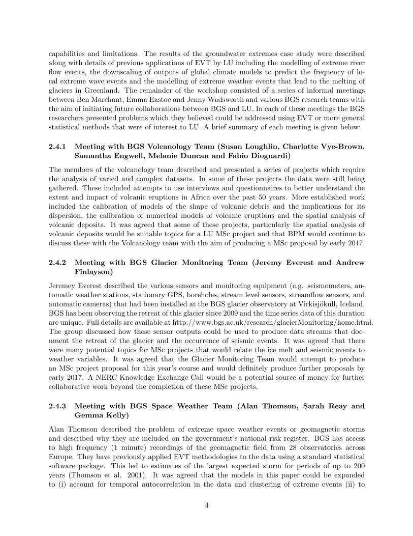
It is common practice in hydrological studies to standardise or normalise time series of precip-itation and water levels before trying to infer relationships between them. In the surface waterliterature this is often achieved by fitting a parametric distribution function to the observations(McKee, 1993). However, Bloomfield and Marchant (2013) demonstrated that GWLs were lesslikely to conform to standard probability distribution functions and therefore used an empiricalapproach to transform the GWLs at a site to a normalised variable which they referred to as theStandardised Groundwater Index (SGI). Seasonal effects are removed from the GWL record byapplying a different transformation to each calendar month. The monthly SGI for Chilgrove Houseand Dalton Holme are shown in Figures 3 and 4. A similar methodology can be used to calculatethe Standardised Precipitation Index (SPI) or if the PE is subtracted from the precipitation theStandardised Effective Precipitation Index (SPEI). However, extreme events in hydrological sys-

7

Figure 1: Observations of GWL, precipitation and PE for Chilgrove House.

Figure 2: Observations of GWL, precipitation and PE for Dalton Holme.

8

Figure 3: SGI (top), SPI (middle) and SPEI (bottom) for Chilgrove House. Accumulation periodfor SPI and SPEI is chosen to maximise correlation with SGI.

tems are often driven by precipitation deficits and excesses over periods longer than a single month.Therefore, prior to normalization the precipitation is summed over an accumulation period of aspecified number of months.

Droughts are generally defined in terms of a deviation from the seasonal norm. This can beachieved by placing a threshold on the standardised index. For instance, McKee (1993) suggestedan SPI between 0 and -1 indicated a mild drought; between -1 and -1.5 indicated a moderatedrought; between -1.5 and -2 indicated a severe drought and less than -2 indicated an extremedrought. Water levels that are higher than the seasonal average can be defined similarly. However,it may be more helpful to define high groundwater levels in terms of absolute levels since these canand have been used to trigger warnings of potential groundwater flooding (Adams et al., 2010).

Studies of the variation of GWLs tend to attempt to model the entire hydrograph rather thanto specifically focus of the extremes. For a number of boreholes, Bloomfield and Marchant (2013)considered the correlation between the SGI and the corresponding SPI or SPEI with various ac-cumulation periods. They demonstrated that the accumulation period that led to the maximumcorrelation was an indicator of the range of the temporal correlation in the SGI. The SEPI (whichaccounts for PE) was slightly more strongly correlated to SGI than the SPI. The plots of theSPI and SPEI that are most strongly correlated with SGI (accumulation periods of 6 months forChilgrove House and 10 months for Dalton Holme) are included in Figures 5 and 6.

One approach that has been used to look for specifically at GWL extremes has been proposed byWilby et al., (2015). They assumed that the occurrence or non-occurrence of a drought (or flood)each month was the outcome of a two-state first order Markov process. The transition probabilitiesof either moving from drought to non-drought or non-drought to drought each month are estimatedfrom the observational record. Then long-term sequences of the drought (or flood) indicator aresimulated and various properties of the extreme event are extracted from these simulations. Forexample, the histrograms in Figures 7 and 8 indicate the probability distribution of the length of a

9

Figure 4: SGI (top), SPI (middle) and SPEI (bottom) for Dalton Holme. Accumulation period forSPI and SPEI is chosen to maximise correlation with SGI.

Figure 5: Correlation between SPI (black) or SPEI (red) and SGI against accumulation period forChilgrove House.

10

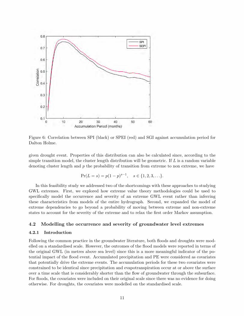
Figure 6: Correlation between SPI (black) or SPEI (red) and SGI against accumulation period forDalton Holme.

given drought event. Properties of this distribution can also be calculated since, according to thesimple transition model, the cluster length distribution will be geometric. If L is a random variabledenoting cluster length and p the probability of transition from extreme to non extreme, we have

Pr(L = s) = p(1− p)s−1, s ∈ {1, 2, 3, . . .}.

In this feasibility study we addressed two of the shortcomings with these approaches to studyingGWL extremes. First, we explored how extreme value theory methodologies could be used tospecifically model the occurrence and severity of an extreme GWL event rather than inferringthese characteristics from models of the entire hydrograph. Second, we expanded the model ofextreme dependencies to go beyond a probability of moving between extreme and non-extremestates to account for the severity of the extreme and to relax the first order Markov assumption.

4.2 Modelling the occurrence and severity of groundwater level extremes

4.2.1 Introduction

Following the common practice in the groundwater literature, both floods and droughts were mod-elled on a standardised scale. However, the outcomes of the flood models were reported in terms ofthe original GWL (in metres above sea level) since this is a more meaningful indicator of the po-tential impact of the flood event. Accumulated precipitation and PE were considered as covariatesthat potentially drive the extreme events. The accumulation periods for these two covariates wereconstrained to be identical since precipitation and evapotranspiration occur at or above the surfaceover a time scale that is considerably shorter than the flow of groundwater through the subsurface.For floods, the covariates were included on their original scale since there was no evidence for doingotherwise. For droughts, the covariates were modelled on the standardised scale.

11

Figure 7: Simulated (bar chart) and theoretical (red) distribution of droughts of different lengthfor Chilgrove House.

Figure 8: Simulated (bar chart) and theoretical (red) distribution of droughts of different lengthfor Dalton Holme.

12

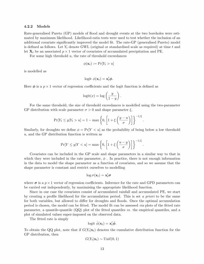
4.2.2 Models

Rate-generalised Pareto (GP) models of flood and drought events at the two boreholes were esti-mated by maximum likelihood. Likelihood-ratio tests were used to test whether the inclusion of anadditional covariate significantly improved the model fit. The rate-GP (generalised Pareto) modelis defined as follows. Let Yt denote GWL (original or standardised scale as required) at time t andlet Xt be an associated p× 1 vector of covariates of accumulated precipitation and PE.

For some high threshold u, the rate of threshold exceedances

φ(xt) := Pr[Yt > u]

is modelled as

logit φ(xt) = x′tφ.

Here φ is a p× 1 vector of regression coefficients and the logit function is defined as

logit(x) = log

(y

1− y

).

For the same threshold, the size of threshold exceedances is modelled using the two-parameterGP distribution with scale parameter σ > 0 and shape parameter ξ,

Pr[Yt ≤ y|Yt > u] = 1−max

{0,

[1 + ξ

(y − uσ

)]}−1/ξ.

Similarly, for droughts we define φ = Pr[Y < u] as the probability of being below a low thresholdu, and the GP distribution function is written as

Pr[Y ≤ y|Y < u] = max

{0,

[1 + ξ

(u− yσ

)]}−1/ξ.

Covariates can be included in the GP scale and shape parameters in a similar way to that inwhich they were included in the rate parameter, φ . In practice, there is not enough informationin the data to model the shape parameter as a function of covariates, and so we assume that theshape parameter is constant and restrict ourselves to modelling

log σ(xt) = x′tσ

where σ is a p× 1 vector of regression coefficients. Inference for the rate and GPD parameters canbe carried out independently, by maximising the appropriate likelihood function.

Since in our case the covariates consist of accumulated rainfall and accumulated PE, we startby creating a profile likelihood for the accumulation period. This is set a priori to be the samefor both variables, but allowed to differ for droughts and floods. Once the optimal accumulationperiod is chosen, the model can be fitted. The model fit can be assessed via plots of the fitted rateparameter, a quantile-quantile (QQ) plot of the fitted quantiles vs. the empirical quantiles, and aplot of simulated values super-imposed on the observed data.

The fitted rate is simplylogit φ(xt) = x′tφ.

To obtain the QQ plot, note that if G(Yt|xt) denotes the cumulative distribution function for theGP distribution, then

G(Yt|xt) ∼ Unif(0, 1)

13

and so− log[1−G(Yt|xt)] ∼ Exponential(1)

We can therefore plot − log[1−G(yt|xt)] against the theoretical quantiles from an Exponential(1)distribution to obtain a QQ plot.

Simulation relies on having a set of covariates x∗. Given these covariates, we can then estimatethe rate function φ(x∗). To decide whether or not the corresponding GWL will exceed the thresholdu, simulate a uniform random variable v ∼ Unif(0, 1). If v < φ(x∗), then the corresponding GWLwill be a threshold exceedances. This can then be simulated from the GP distribution, withparameters σ(x∗, ξ), using the probability integral transform method. Under the model definedabove we have no model for non-exceedances and no way of simulating these; neither does thesimulation method account for any serial dependence in the GWLs.

Having estimated the covariate model, the marginal distribution of the data set can be trans-formed to a common distribution to aid modelling of the lag 1 dependence structure. The stan-dardised GWL must first be transformed to Uniform margins on [0, 1] using the transformation

F (Yt) =

φD(xt)

[1 + ξD

(uD−YtσD(xt)

)]−1/ξDYt < uD

F (Yt) uD ≤ yt ≤ uF1− φF (xt)

[1 + ξF

(Yt−uFσF (xt)

)]−1/ξDYt > uF

where F denotes the empirical distribution function; φD(·), σD(·) and ξD are the fitted rate andGP scale and shape parameters for droughts; φF (·), σF (·) and ξF are the fitted rate and GP scaleand shape parameters for floods; and uD (uF ) is the modelling threshold for droughts (floods).From Uniform margins this can be moved to any desired margin for modelling (common choicesare Laplace, Frechet or Gumbel).

4.2.3 Results

Chilgrove House: The empirical 0.1 and 0.9 quantiles of the standardised GWL data were usedto define droughts and floods respectively. For the Chilgrove House drought model, the optimalprecipitation and PE accumulation period is 0-8 months (where 0 months means the month in whichthe threshold exceedance occurred). For the corresponding floods model, the optimal precipitationand PE accumulation period is 0-2 months. Plots of the profile likelihoods for these periods aregiven in Figure 9. These different accumulation periods are consistent with the observation ofEltahir and Yeh (1999) that groundwater drought episodes tend to be more prolonged than floods.The corresponding exceedance probabilities are plotted in Figure 10.

Examples of data simulated from both drought and flood models are given in Figure 11. Inboth cases the covariates used in simulation were the observed covariates. Simulated data are givenon the standardised scale (droughts) and the original scale (floods). For the floods, because themodel was fitted on the standardised scale, the simulated values had to be transformed back to theoriginal scale using observed monthly means and standard deviations of the GWL.

Figure 12 shows the dependence between successive monthly observations once the data havebeen transformed to Laplace margins. The first figure shows the data as a time series, the second isa scatter plot of the observations at lag t against the observations at lag t− 1. This transformationappears to lead to a more symmetric behaviour in the dependence structure than that observed bytransforming without accounting for covariates directly.

14

●

●

●

●

●

●

●●

●● ●

●

●

0 2 4 6 8 10 12

−40

0−

350

−30

0−

250

Cumulation Period

Pro

file

log−

likel

ihoo

d

●

●

●

●

●

●

●

●

●

●

●

●

●

0 2 4 6 8 10 12

−60

0−

550

−50

0

Cumulation Period

Pro

file

log−

likel

ihoo

d

Figure 9: Profile likelihoods for accumulation period (months) for threshold exceedance models:droughts (left) and floods (right).

1920 1940 1960 1980 2000

0.0

0.2

0.4

0.6

0.8

1.0

Time

Rat

e

1920 1940 1960 1980 2000

0.0

0.2

0.4

0.6

0.8

1.0

Time

Rat

e

Figure 10: Estimated probability of a threshold exceedance for droughts (left) and floods (right).

15

1920 1940 1960 1980 2000

−2

02

4

Date

GW

L

●●●

●

●●●●●

●

●●● ●

●

●●●

●

●

●

●

●

●●●

●●

●

●

●

●

●

●

●●

●●

●●●

●

●●

●

●●

●

●

●●

●

●●●

●● ●

●●●●

●

●

●

●

●

●

●

●

●

●

●

●

●

●

●●●

●

●

●●

●●

●●●

●

●

●

●

●

●●

●

●●

●●● ●

●●

●

●●

●

●

●●

●●●●●

●●●

1920 1940 1960 1980 2000

4050

6070

8090

Date

GW

L

●

●

●

●

●

●

●

●

●

●●

●

●

●

●

●

●

●

●

●

●

●

●

●

●

●

●

●

●

●

●

●●

●

●

●●

●

●

●

●

●

●

●●

●●

●

●

●

●

●

●

●

●

●

●

●

●

●●

●

●

●

●

●●

●

●

●

●

●

●

●

●

●

●

●

●

●

●

●●

●●

●

●●

●

●

●

●

●

●

●

●

●

●●

●

●●

●

●

●

●

●

●

●

●

●

●●

●

●

●

●

●

●

●

Figure 11: Simulated data (red circles) for droughts (left) and floods (right). Black lines show theobserved GWL on the standardised (drought) and original (flood) scales.

1920 1940 1960 1980 2000

−5

05

Time

GW

L (L

apla

ce)

●

●

●●

●●

●●●● ●

●

●●

●

●

●

●●

●

●

●

●

●

●

●

●

●

●

●

●

●

●

●●●

●

●

●

●●

●●●

●●

●

●

●

●

●

●●●●●

●● ●

●

●●

●

●●

●●●●

●●

●

●

●

●●●●● ●

●

●

●

●

●

●●● ●

●●●●

●●

●

●●

●●

●

●●●

●

●

●●

●●

●

●

●● ●

●●

●

● ●

●

●

●

●

●

●

●●●●

●

●

●

●

●

●●●●●

●●

●

●

●

●●●

●●●

●

●●● ●

●

●

●●

●

●

●●

●

●●

●

●

●●

●

●

●

●●

● ●

●

●

●●

●

● ●

●

●●

●

●●●

●

●

●

●

●

● ●

●

●

● ●

●

●●

●

●●●●●

●●

●

●

●●

●

●●

●

●●● ●

●

●

●

●

●

●●●●

●●

●●

●

●

●

●●

●●

●●●

●

●●

●

●

●●

●

●

●

●

●

●

●

●

●

●

●

●

●●●●●

●

●

●

●●

●●

●

●●

●

●●

●

●

●

●

●●

●●●●

●

●

●●

●

●

●

●●●●●

●●● ●

●●

●●

●

●

●●

●

●

● ●

●●

●

●

●●●●●●

●

●

●

●

●●●●●●●

●

●

●

●

●

●

●

●●●●

●●

●

●●

●

●

●●

●●●

●●

●

●●

●

●

●●●●●●●● ●

●●

●

●●

●● ●

●●

●●

●

●●●

●●● ●

●●

●

●

●

●

●

●● ●

●

●●●

●●

●

●

●● ●

●●

●

●

●●

●●

●

●

●

●●●

●●

●

●

●

●

●●

●

●

●

●

●

●●

●●●

●●●●●●

●●

●●●

●

●

●●●●●●● ●

●●

●

●

●●●

●● ●

●

●

●

●

●

●●

●●

●●

●●

●●

●●

●●● ●

●

●●

●●●

●

●

●

●●●●

●●●

●

●

●

●

●

●

● ●

●

●●

●

●

● ●

●●

●

●●

●●

●

●●

●

● ●

●

●

●●●●●●●

●●

●●●●● ●

●●

●●

●

●

●

●

● ●

●●●●●●

●

●

●

●●●

●● ●

●●

●

●

●

●●

● ●

●●

●●

●

●

●●

●●

● ●●●●●●●●

●

●

●

●

●

●

●

●

●

●●

●

●

●

●

●●

●●

●

●

●

●

●●

●

●

●

●●●●

●

●●

●

●

●

●

●

●

●

● ●●

●

●

●

●●

●

●

● ●

●●

●

●●

●●●

●●

●

●

●

●

●

●

●

● ●

●

●

●

●● ●●

●●●

●

●●

●●

●●

●

●

●● ●

●

●

●

●●●● ●

●●

●●

●

●●

●●

●●●●●

●●

●●● ●

●●

●

●

●

●●●

● ●

●

●

●

●●

●●

●

● ●

●

●

●

●●

●●

●

●●

●●

●

●●

●●

●

●

●●●

●

●

●●

●

●

●

●

●●●

●●

●●

●●●

●

●

●

●

●

●

●●

● ●

●

●

●

●

●

●●

●

●

●●

●

●

● ●

●

●●●

● ●●

●

●

●

●

●

●

●

●

●

●

●

●

●●

●

●

●

●●

●●●

●

● ●

●

●

●

●

●

●●

●

●

●

●

● ●

●●

●

●●

●

●●

●●

●

●

●●

●

●

●●●

●

●

●

● ●

●

●

●

●

●●●

●

●●

●

●

●

●

●

●

●

●●●

●

●●

●

●

●

●●●

●●●

●●

●

●

●●

●●●

●

●

●

● ●

●

●

●

●●

●

●

●

●

●

●●

●

●●

●

●

●

●●

●

●

●

●

●

●●

●

●●

●●

●

●

● ●

●

●●

●

●●

●●●● ●

●

●

●

●●

●

●

●●●

●

●●

●

●●

●●

●

●

●

●●●●

●

●●●

●●●● ●

●●●●

●

● ●

●●

●

● ●

●●

●●

●

●

●

●

●

●

●●●● ●

●●

●

●

●●●●

●●

●

●●

●

●

● ●

●

●●

●

●

●

●

●

●

●

●

●●

●

●

●●

●

●●● ●

●●

●

●

●

●

●

●

●

●

●

●

●

●

●

●

●

●

●

●●

●

●

●●

● ●

●

●●

●●●●

●●●

●

●

●

●

●

●

● ●

●●

●

● ●

● ●

●●

●

●● ●

●●

●●

●

●

●

● ●

●

●●

●●

●

●

●

●

●

●●●

●●● ●

●

●

●●

●

●

●

● ●

●

●

●

● ●

●

●

●

● ●●

●

●

●

●

●●

●

●

●

●

●

●●

●

●●

●

−5 0 5

−5

05

Xt

Xt−

1

Figure 12: GWL transformed to common Laplace margins: time series (right-hand side) and lag 1dependence (left-hand side).

16

●

●

●

●

●

●

●

●

●

●

●

●● ● ● ●

●

●

●

●

0 5 10 15

−45

0−

400

−35

0−

300

Cumulation Period

Pro

file

log−

likel

ihoo

d

●

●

●

●

●●

●

●

●

●

●●

●

0 2 4 6 8 10 12

−40

0−

350

−30

0−

250

Cumulation Period

Pro

file

log−

likel

ihoo

d

Figure 13: Dalton Holme: profile likelihoods for cumulation period for threshold exceedance models:droughts (left) and floods (right).

Dalton Holme: The analyses were repeated for Dalton Holme. Here the optimal precipitationand PE accumulation periods were 0-15 months (droughts) and 0-4 months (floods). It shouldbe noted from the plots in Figure 13 that the profile likelihood for the accumulation period fordroughts is fairly flat, particularly between 11 and 16 months. Plots of the rate parameters andsimulated values for both droughts and floods are given in Figure 14 and 15 for probabilities andsimulations respectively.

4.3 Exploratory extremal dependence analysis in groundwater time series

Exploratory extremal dependence analyses were carried out to gather an initial assessment on thenature of the extremal dependence in both tails of the GWL time series, {Yt}. This focussed onuse of two summary measures, applied to pairs of consecutive observations (Yt, Yt+1).

The first summary is the coefficient of tail dependence, (Ledford and Tawn, 1996). Supposethat (X1, X2) are two random variables with standard exponential marginal distributions (i.e.Pr(X1 > x) = Pr(X2 > x) = e−x, x > 0); this is achieved approximately in practice via marginaltransformations. Then the coefficient of tail dependence is defined as the parameter η ∈ (0, 1], inthe model

Pr(X1 > x,X2 > x) = Pr(min(X1, X2) > x) = Ce−x/η, C > 0,

which is assumed to hold for x > x∗, where x∗ is a high quantile (often the 90% or 95% quantile).Larger values of η correspond to stronger extremal dependence, with η < 0.5, η ≈ 0.5, η > 0.5corresponding to negative extremal association, near extremal independence, and positive extremalassociation, respectively. The value η = 1 plays a special role, as this suggests that the data areasymptotically dependent, which roughly means that there will always be a positive probability ofobserving joint extremes of (Yt, Yt+1), whatever the level of the extremes.

A complementary measure of extremal dependence is the measure χ(u), defined for two variables(U, V ) with standard uniform marginal distributions (i.e. Pr(U > u) = Pr(V > u) = 1 − u, 0 <

17

1920 1940 1960 1980 2000

0.0

0.2

0.4

0.6

0.8

1.0

Time

Rat

e

1920 1940 1960 1980 2000

0.0

0.2

0.4

0.6

0.8

1.0

Time

Rat

e

Figure 14: Dalton Holme: Estimated probability of a threshold exceedance for droughts (left) andfloods (right).

1920 1940 1960 1980 2000

−4

−2

02

4

Date

GW

L

●

●

●

●

●

●

●

●

●

●●●

●

●

●

●

●

●

●

●●

●●●●●

●

●

●

●

●

●

●

●

●●

●

●●●

●

●

●

●

●

●

●

●

●

●

●●●●

●

●

●

●

●

●

●●

●

●

●

●

●

●

●

●

●

●

●●

●

●

●●

●●

●

●

●

● ●●

●

●

●●●

●●

●

●

●

●

●●

●

●

●

●

●

●

●

●

●

●

●

●

●

●

●

●

●●●●

●

●●

●●

●

●

●

●●●

●

●

●

●

●●

●

1920 1940 1960 1980 2000

1015

2025

Date

GW

L

●

●●

●

●

●

●

●

●

●●●

●

●

●

●

●

●

●

●

●

●

●

●

●

●

●

●

●

●

●

●

●

●

●● ●

●

●●

●

●

●

●

●

●●

●

●●

●●

●

●

●

●●

●

●

●●

●●●

●

●

●

●

●

●

●

● ●●

●

●

●

●

●

●

●

●

●

●

●

●

●

●

●

●

●

●●●●

●●

●

●

●

●

●

●

●

●

●

●

●

●

●

●

●

●

Figure 15: Dalton Holme: Simulated data (red circles) for droughts (left) and floods (right). Blacklines show the observed GWL on the standardised (drought) and original (flood) scales.

18

u < 1) as

χ(u) =Pr(U > u, V > u)

1− u.

Of particular interest is the behaviour of χ(u) as u approaches 1, as if this remains positive, thisis indicative of asymptotic dependence (η = 1), whilst if it tends to zero, this is indicative ofasymptotic independence (η < 1). Canonically both these summary measures focus on the uppertail, thus when we wanted to estimate them in the context of the lower tail, we transformed thelower tail to be the upper tail, which is achieved by applying a monotonically decreasing marginaltransformation.

In this initial stage of exploratory extremal dependence analysis, marginal transformation tookaccount of the value of the PE covariate, as exploratory plots revealed this to have a notableimpact on the lag 1 dependence structure. Tentative conclusions were that the lag 1 dependencewas stronger in the lower tail than the upper tail and that the value of PE had some effect on thelevel of dependence; in particular lower tail dependence was stronger for larger values of PE. Thesefindings are consistent with our understanding of the groundwater system. Droughts are less likelyto break because for GW to recharge and lead to GWL rise the soil needs to wet up and wettedpathways from the surface to the water table need to be developed first before rainfall can becomeeffective in leading to GWL rise. Whereas under high GWL stands as soon as rainfall stops thesystem will drain and GWLs will fall.

During the exploratory extremal dependence analysis, marginal transformations were madeaccording to one of four PE groupings, which somewhat represent seasonality in the data. Analternative way to standardise the data to remove seasonal heterogeneity is to assume that obser-vations from a particular calendar month come from a common distribution. This results in a timeseries of Standardised Groundwater Index, as described in Section 4.1. To go forward and modelthe dependence, we focussed on standardised GWLs and on modelling the lower tail dependence.

4.4 Modelling Lower Tail Dependence of Standardised GWLs

Full statistical models are required to determine the expected duration of an extreme event. Theapproach described below is based on the model of Heffernan and Tawn (2004) which can accountfor dependencies in both forwards and backwards directions and hence also accomodate asymmetryobserved in the data.

4.4.1 Methods

Marginal Transformations The GWL series at Chilgrove House and Dalton Holme were stan-dardised seasonally to uniformity by using the following transform within each month j ∈ {1, . . . , 12}of the data:

Fj(Yt) =

{Fj(Yt) Yt > u∗

H(Yt) Yt < u∗

where Fj denotes the empirical distribution function of the observations in month j, and H is thegeneralised Pareto distribution function fitted to the lower tails pooled across all months (this wasreasonably well supported by diagnostic plots; furthermore fits within individual months of the GPdistribution were quite problematic, due to very short tails in some months).

The resulting time series can then be transformed to any scale desired; we denote the marginallytransformed series by {Xt}. The left panel of Figure 16 shows the time series on a standard normalscale (i.e., each month has been transformed to standard normal), whilst the right panel of Figure 16shows (Xt, Xt+1) on this transformed scale.

19

0 200 400 600 800 1000 1200

−3

−2

−1

01

2

Index

CH

Sta

ndar

dise

d G

WL

serie

s

−3 −2 −1 0 1 2

−3

−2

−1

01

2

Xt

Xt−

1

Figure 16: Left: standardised GWL time series; Right: lag 1 dependence

To analyse the extremal dependence, we transformed to standard exponential margins, withthe lower tail transformed to be the upper tail; see Figure 17. The explicit goal here was to modelthe excursions of the time series over a high threshold (corresponding to low values of the originalseries) using models motivated by extreme value theory. Specifically we adopted a version of themodel of Heffernan and Tawn (2004), recently used in a time series context by Winter and Tawn(2016). We began with a simple assumption that the time series behaves as a first order Markovchain in the extremes (i.e. Xt is independent of Xt−k, k ≥ 2 given Xt−1). This simple analysishelps to illustrate the theory, but appeared to be too restrictive, thus ultimately a slightly moresophisticated model will be described.

0 200 400 600 800 1000 1200

02

46

8

Index

CH

Sta

ndar

dise

d G

WL

serie

s

0 200 400 600 800 1000 1200

02

46

8

Index

CH

Sta

ndar

dise

d G

WL

serie

s

0 2 4 6 8

02

46

8

Xt

Xt−

1

Figure 17: Left: standardised groundwater time series in exponential margins, with upper tail asthe lower tail; Centre: same as left, but with red points highlighting “clusters”; Right: Lag 1dependence in exponential margins.

First order conditional extremes model Heffernan and Tawn (2004) show that for randomvariables in exponential-tailed margins, a broadly valid assumption is

Pr(Xt+1 − αXt

Xβt

≤ x,Xt − u > y | Xt > u)→ G(x)e−y, u→∞,

i.e. large values of Xt become independent of {Xt+1 − αXt}/Xβt , which follow some unknown

non-degenerate distribution G. When the variables have Laplace margins, the parameters α ∈[−1, 1], β ∈ (−∞, 1). If instead exponential margins are used and dependence is non-negative,

20

then α ∈ [0, 1]; this constraint was implemented in the fits described below. In either case, theparameters α, β may be estimated by maximum likelihood under a false working assumtion thatG is Gaussian; confidence intervals may be obtained through bootstrap procedures, but we donot consider this here. Using the maximum likelihood estimates (MLEs) of α, β, the residuals

Z = {Xt+1 − αXt}/X βt can be calcuated, and their empirical distribution used to approximate G.

The main reason for fitting a model is to infer characteristics of the extremes: here this isachieved through simulation from the fitted model. To simulate new values of (Xt, Xt+1)|Xt > u,denoted (Xt, Xt+1), the following algorithm was used:

Algorithm 1

1. Draw Xt ∼ Exp(1) + u

2. Draw a value Zi from the empirical distribution of residuals (with replacement)

3. Set Xt+1 = αXt + X βt Zi

0 2 4 6 8

02

46

8

fit$dat[,1]

fit$d

at[,2

]

Figure 18: Lag 1 dependence at Chilgrove House in standard exponential margins (black points)with new values simulated (red points)

Algorithm 1 is illustrated in Figure 18. Under the assumption that the time series is first orderMarkov, a simulation scheme like this can be iterated to produce a chain of values (Xt, Xt+1, . . . , Xt+l)larger than a high threshold u. Specifically,

Algorithm 2

1. Draw Xt ∼ Exp(1) + u. Set k = 0.

2. While Xt+k > u:

• Draw a value Zi from the empirical distribution of residuals (with replacement)

• Xt+k = αXt−k + X βt−kZi

• Set k → k + 1

Else stop

21

3. Return the tail chain (Xt, . . . , Xt+l).

Algorithm 2 describes how to simulate a tail chain in a forwards direction, but this proce-dure could also be done in the other direction, i.e. simulating backwards. This approach and itsapplication to Chilgrove House is described in Section 4.4.3.

To determine if this model is adequate for the tails of the transformed GWL time series, weused repeated simulation to assess its ability to capture the characteristics of the observed data.Specifically we focussed on three characteristics: (i) cluster length; (ii) cluster maximum; (iii)average value of exceedances. Clusters here were defined as groups of uninterrupted thresholdexceedances. Alternatively one could use the Runs method (Smith and Weissman, 1994), wherebythreshold exceedances followed by a run of at least m consecutive non-exceedances are deemed tobe in separate clusters, else they are deemed to be in the same cluster.

4.4.2 Results

Comparison of cluster characteristics: Chilgrove House The first-order Markov condi-tional extremes model was used to create 1000 simulated clusters at various thresholds. Figures 19-21 display histograms of the summaries (i), (ii) and (iii), whilst Tables 1-3 gives the average value ofthese summaries. In both the figures and tables the first row corresponds to the observed data, thesecond to the simulated data from the first-order Markov conditional extremes model. The thirdrow corresponds to the methodology to be described in Section 4.4.3. (Note the differing scales onthe histograms.) Numbers in parentheses are the standard deviations of the observed means.

Threshold u = 2 Number of observed clusters: 47.

22

Mean cluster length Mean cluster maximum Mean cluster meanObserved 3.40 (0.45) 3.31 (0.20) 2.75 (0.09)Simulated 4.4 3.83 3.13Simulated (second order) 4.62 3.58 3.07

Table 1: Observed and simulated cluster characteristics with threshold u = 2

Observed cluster lengths u= 2

Cluster length

Den

sity

0 2 4 6 8 10 12 14

0.00

0.05

0.10

0.15

0.20

0.25

Observed cluster maxima u= 2

Cluster max

Den

sity

2 3 4 5 6 7 8

0.0

0.1

0.2

0.3

0.4

0.5

Observed cluster mean u= 2

Cluster mean

Den

sity

2.0 2.5 3.0 3.5 4.0 4.5 5.0

0.0

0.2

0.4

0.6

0.8

Simulated cluster lengths u= 2

Cluster length

Den

sity

0 5 10 15 20 25 30

0.00

0.05

0.10

0.15

0.20

Simulated cluster maxima u= 2

Cluster max

Den

sity

5 10 15

0.0

0.1

0.2

0.3

0.4

Simulated cluster mean u= 2

Cluster mean

Den

sity

2 3 4 5 6 7 8

0.0

0.1

0.2

0.3

0.4

0.5

0.6

Simulated cluster lengths (2nd order) u= 2

Cluster length

Den

sity

0 5 10 15 20 25

0.00

0.05

0.10

0.15

0.20

Simulated cluster maxima (2nd order) u= 2

Cluster max

Den

sity

2 4 6 8 10

0.0

0.1

0.2

0.3

Simulated cluster mean (2nd order) u= 2

Cluster mean

Den

sity

2 3 4 5 6 7 8

0.0

0.1

0.2

0.3

0.4

0.5

0.6

Figure 19: Observed and simulated cluster characteristics with threshold u = 2

Threshold u = 2.25 Number of observed clusters: 44.

23


Table 2: Observed and simulated cluster characteristics with threshold u = 2.25

Observed cluster lengths u= 2.25

Cluster length

Den

sity

0 2 4 6 8 10 12

0.00

0.05

0.10

0.15

0.20

0.25

0.30

Observed cluster maxima u= 2.25

Cluster max

Den

sity

2 3 4 5 6 7 8

0.0

0.1

0.2

0.3

0.4

0.5

Observed cluster mean u= 2.25

Cluster mean

Den

sity

2.0 2.5 3.0 3.5 4.0 4.5 5.0

0.0

0.2

0.4

0.6

Simulated cluster lengths u= 2.25

Cluster length

Den

sity

0 5 10 15 20

0.00

0.05

0.10

0.15

0.20

0.25

Simulated cluster maxima u= 2.25

Cluster max

Den

sity

2 4 6 8 10 12 14

0.00

0.10

0.20

0.30

Simulated cluster mean u= 2.25

Cluster mean

Den

sity

2 3 4 5 6 7 8 9

0.0

0.1

0.2

0.3

0.4

0.5

Simulated cluster lengths (2nd order) u= 2.25

Cluster length

Den

sity

0 5 10 15 20 25 30 35

0.00

0.05

0.10

0.15

Simulated cluster maxima (2nd order) u= 2.25

Cluster max

Den

sity

2 4 6 8 10 12

0.00

0.10

0.20

0.30

Simulated cluster mean (2nd order) u= 2.25

Cluster mean

Den

sity

2 3 4 5 6 7 8

0.0

0.1

0.2

0.3

0.4

0.5

0.6

Figure 20: Observed and simulated cluster characteristics with threshold u = 2.25


24




Cluster length

Den

sity

0 2 4 6 8 10 12

0.00

0.05

0.10

0.15

0.20

0.25

0.30


Cluster max

Den

sity

2 3 4 5 6 7 8

0.0

0.1

0.2

0.3


Cluster mean

Den

sity

2.5 3.0 3.5 4.0 4.5 5.0 5.5

0.0

0.2

0.4

0.6

0.8


Cluster length

Den

sity

0 5 10 15 20 25 30 35

0.00

0.05

0.10

0.15


Cluster max

Den

sity

2 4 6 8 10

0.00

0.05

0.10

0.15

0.20

0.25

0.30


Cluster mean

Den

sity

3 4 5 6 7 8

0.0

0.1

0.2

0.3

0.4

0.5


Cluster length

Den

sity

0 5 10 15 20 25

0.00

0.05

0.10

0.15

0.20

0.25


Cluster max

Den

sity

2 4 6 8 10

0.00

0.10

0.20

0.30


Cluster mean

Den

sity

3 4 5 6 7

0.0

0.1

0.2

0.3

0.4

0.5


For each threshold, the clusters simulated using the first-order Markov chain appear to be toolong, with the simulated cluster maxima and means are also systematically too large. This datasetwas examined again using backwards simulation, described in Section 4.4.3.

Comparison of cluster characteristics: Dalton Holme The previous analysis was repeatedfor Dalton Holme; the standardised data (Xt, Xt+1), are plotted in Figure 22, with the lower tailas the upper tail. Figures 23-25 and Tables 4-6 summarise the simulations as above.

25

0 2 4 6 8

02

46

8

Xt

Xt+

1

Figure 22: Lag 1 dependence for Dalton Holme in standard exponential margins (black points)with new values simulated (red points)

Threshold u = 2 Number of observed clusters: 28.


Cluster length

Den

sity

0 5 10 15 20 25 30

0.00

0.04

0.08

0.12


Cluster max

Den

sity

2 3 4 5 6 7 8

0.0

0.1

0.2

0.3

0.4

0.5

0.6

0.7


Cluster mean

Den

sity

2.0 2.5 3.0 3.5 4.0 4.5 5.0

0.0

0.2

0.4

0.6

0.8

1.0

Simulated cluster lengths u= 2

Cluster length

Den

sity

0 20 40 60 80 100 120

0.00

0.02

0.04

0.06

Simulated cluster maxima u= 2

Cluster max

Den

sity

2 4 6 8 10 12 14

0.0

0.1

0.2

0.3

Simulated cluster mean u= 2

Cluster mean

Den

sity

2 3 4 5 6 7 8

0.0

0.1

0.2

0.3

0.4

0.5

0.6

Simulated cluster lengths (2nd order) u= 2

Cluster length

Den

sity

0 10 20 30 40 50 60

0.00

0.02

0.04

0.06

0.08

0.10

Simulated cluster maxima (2nd order) u= 2

Cluster max

Den

sity

2 4 6 8 10

0.0

0.1

0.2

0.3

0.4

Simulated cluster mean (2nd order) u= 2

Cluster mean

Den

sity

2 3 4 5 6

0.0

0.1

0.2

0.3

0.4

0.5

0.6

0.7

Figure 23: Observed and simulated cluster characteristics with threshold u = 2


26


Table 4: Observed and simulated cluster characteristics with threshold u = 2




Cluster length

Den

sity

0 5 10 15 20 25 30

0.00

0.02

0.04

0.06

0.08

0.10

0.12


Cluster max

Den

sity

2 3 4 5 6 7 8

0.0

0.1

0.2

0.3

0.4

0.5

0.6


Cluster mean

Den

sity

2.0 2.5 3.0 3.5 4.0 4.5 5.0

0.0

0.2

0.4

0.6

0.8


Cluster length

Den

sity

0 20 40 60 80 100

0.00

0.02

0.04

0.06


Cluster max

Den

sity

5 10 15

0.00

0.05

0.10

0.15

0.20

0.25

0.30


Cluster mean

Den

sity

2 3 4 5 6 7 8

0.0

0.1

0.2

0.3

0.4

0.5

0.6


Cluster length

Den

sity

0 10 20 30 40

0.00

0.02

0.04

0.06

0.08

0.10


Cluster max

Den

sity

2 4 6 8 10

0.0

0.1

0.2

0.3


Cluster mean

Den

sity

2 3 4 5 6

0.0

0.2

0.4

0.6



27




Cluster length

Den

sity

0 5 10 15 20 25 30

0.00

0.04

0.08

0.12


Cluster max

Den

sity

2 3 4 5 6 7 8

0.0

0.1

0.2

0.3

0.4


Cluster mean

Den

sity

2.5 3.0 3.5 4.0 4.5 5.0 5.5

0.0

0.2

0.4

0.6

0.8

1.0

1.2


Cluster length

Den

sity

0 20 40 60 80 100

0.00

0.02

0.04

0.06


Cluster max

Den

sity

5 10 15 20

0.00

0.05

0.10

0.15

0.20

0.25

0.30


Cluster mean

Den

sity

2 4 6 8 10 12

0.0

0.1

0.2

0.3

0.4


Cluster length

Den

sity

0 10 20 30 40 50

0.00

0.02

0.04

0.06

0.08

0.10

0.12


Cluster max

Den

sity

2 4 6 8 10

0.0

0.1

0.2

0.3

0.4


Cluster mean

Den

sity

3 4 5 6 7

0.0

0.2

0.4

0.6


As with Chilgrove House, the first order model overestimated cluster lengths, maxima andmeans. We now describe a proposal to improve the model.

4.4.3 Extensions

Second order conditional extremes model As the first order model did not capture thecluster characteristics well, we proposed a modification that allows for some consideration of theprevious two values of the chain. The motivation for this came from exploratory analysis of thepartial autocorrelation function (PACF), calculated from the data on the Gaussian scale, which forboth the Chilgrove House and Dalton Holme shows negative dependence at lag 2.

28

0 5 10 15 20 25 30

0.0

0.2

0.4

0.6

0.8

Lag

Par

tial A

CF

PACF for CH data, Gaussian scale

0 5 10 15 20 25 30

−0.

20.

00.

20.

40.

60.

8

Lag

Par

tial A

CF

PACF for DH data, Gaussian scale

Figure 26: PACFs for Chilgrove House and Dalton Holme

Although the PACFs include dependence throughout the body as well as the tails, Figure 26hints at the possibility of negative dependence between (Xt, Xt+2)|Xt+1 (although positive de-pendence unconditionally). One way to assess whether there is indeed negative dependence inthe extremes is to perform both conditional extremes fits both one step forwards and one stepbackwards and examine association in the residuals. Figure 27 displays these for Dalton Holme,confirming negative association (Kendall / Spearman / Pearson correlations: −0.23/−0.34/−0.33).

−0.5 0.0 0.5

−0.

50.

00.

51.

01.

5

Zf

Zb

Figure 27: DH: One step forwards and backwards residuals

In order to account for this, we proposed the following novel algorithm:

Algorithm 3

1. Use the one step forwards conditional fit (with parameters (αF , βF )) and calculate residuals

ZF = {Xt+1 − αFXt}/X βFt

2. Use the one step backwards conditional fit (with parameters (αB, βB)) and calculate residuals

ZB = {Xt − αBXt+1}/X βBt+1

3. Concatenate forwards–backwards residuals (ZF , ZB)

4. Draw Xt ∼ Exp(1) + u

5. Draw a value ZF from the empirical distribution of forwards residuals (with replacement)

29

6. Set Xt+1 = αF Xt + X βFt ZF

7. Use (αB, βB) to find the corresponding backwards residual ZB = {Xt − αBXt+1}/X βBt+1

8. Sample the next residual ZF |ZB (see below for a possible method)

9. Proceed as in Algorithm 2, but at each step following items 6–8 to ensure conditional samplingof ZF .

To sample ZF |ZB, we adopted the simplest method of using “nearest neighbours” in the ZBspace. That is, for a chosen value of m, we selected the m nearest values of ZB to ZB, and sampledthe next ZF only from those associated to the relevant ZB values. This is illustrated in Figure 28.A more sophisticated approach would be to use kernel density estimation to produce weights forthe conditional sampling, but this was not considered further here. Following this approach, if wesimulate a large value Xt+1, then this leads to a larger value of ZB, which in turn means we samplesmaller values of ZF for the next step forwards, resulting in shorter chains.

−0.5 0.0 0.5

−0.

50.

00.

51.

01.

5

Zf

Zb

Figure 28: DH: One step forwards and backwards residuals, with conditional sampling illustratedfor m = 30. Blue line indicates the value of ZB, red dots show the values of ZF that can be sampledfor the next value.

The results of applying this second order algorithm are given in Section 4.4.2 for Chilgrove Houseand Dalton Holme, in the third rows of the tables and figures (withm = 20 nearest neighbours used).For Chilgrove House, the effect is small, which perhaps reflects the fact that the negative correlationin the forward–backwards residuals is not as strong (Kendall / Spearman / Pearson correlations atu = 2: −0.095/−0.12/−0.10) as that of Dalton Holme, where reasonable improvements are noted.

Backward simulation for Chilgrove House Neither the first nor second order simulationschemes for Chilgrove House appeared to satisfactorily capture the empirical characteristics of thesample. Noting that these data have a higher degree of asymmetry than the Dalton Holme data, wealso experimented with backwards simulation. Figures 30-32 and Tables 7-9 are as in section 4.4.2,except the second row now corresponds to first order backwards simulation. Figure 29 displays thelag 1 values, beginning with Xt+1 > u.

30

Mean cluster length Mean cluster maximum Mean cluster meanObserved 3.40 (0.45) 3.31 (0.20) 2.75 (0.09)Simulated (backwards) 3.96 3.47 2.84

Table 7: Observed and backwards simulated cluster characteristics with threshold u = 2

0 2 4 6 8

02

46

8

Xt

Xt+

1

Figure 29: Lag 1 dependence for Chilgrove House in exponential margins (black points) with newvalues simulated (red points)

Threshold u = 2


Cluster length

Den

sity

0 2 4 6 8 10 12 14

0.00

0.05

0.10

0.15

0.20

0.25


Cluster max

Den

sity

2 3 4 5 6 7 8

0.0

0.1

0.2

0.3

0.4

0.5


Cluster mean

Den

sity

2.0 2.5 3.0 3.5 4.0 4.5 5.0

0.0

0.2

0.4

0.6

0.8

Simulated cluster lengths (backward) u= 2

Cluster length

Den

sity

0 5 10 15 20 25

0.00

0.05

0.10

0.15

0.20

Simulated cluster maxima (backward) u= 2

Cluster max

Den

sity

2 4 6 8 10

0.0

0.1

0.2

0.3

0.4

Simulated cluster mean (backward) u= 2

Cluster mean

Den

sity

2 3 4 5 6

0.0

0.1

0.2

0.3

0.4

0.5

0.6

0.7

Figure 30: Observed and backwards simulated cluster characteristics with threshold u = 2

Threshold u = 2.25

31

Mean cluster length Mean cluster maximum Mean cluster meanObserved 2.66 (0.38) 3.44 (0.20) 3.00 (0.10)Simulated (backward) 2.96 3.46 3.02

Table 8: Observed and backwards simulated cluster characteristics with threshold u = 2.25


Cluster length

Den

sity

0 2 4 6 8 10 12

0.00

0.05

0.10

0.15

0.20

0.25

0.30


Cluster max

Den

sity

2 3 4 5 6 7 80.

00.

10.

20.

30.

40.

5


Cluster mean

Den

sity

2.0 2.5 3.0 3.5 4.0 4.5 5.0

0.0

0.2

0.4

0.6

Simulated cluster lengths (backward) u= 2.25

Cluster length

Den

sity

2 4 6 8 10 12 14

0.0

0.1

0.2

0.3

0.4

0.5

Simulated cluster maxima (backward) u= 2.25

Cluster max

Den

sity

2 4 6 8

0.0

0.1

0.2

0.3

0.4

0.5

Simulated cluster mean (backward) u= 2.25

Cluster mean

Den

sity

2 3 4 5 6

0.0

0.1

0.2

0.3

0.4

0.5

0.6

0.7

Figure 31: Observed and backwards simulated cluster characteristics with threshold u = 2.25

Threshold u = 2.5


Cluster length

Den

sity

0 2 4 6 8 10 12

0.00

0.05

0.10

0.15

0.20

0.25

0.30


Cluster max

Den

sity

2 3 4 5 6 7 8

0.0

0.1

0.2

0.3


Cluster mean

Den

sity

2.5 3.0 3.5 4.0 4.5 5.0 5.5

0.0

0.2

0.4

0.6

0.8

Simulated cluster lengths (backward) u= 2.5

Cluster length

Den

sity

0 5 10 15 20

0.00

0.05

0.10

0.15

0.20

0.25

0.30

Simulated cluster maxima (backward) u= 2.5

Cluster max

Den

sity

2 4 6 8 10 12

0.0

0.1

0.2

0.3

Simulated cluster mean (backward) u= 2.5

Cluster mean

Den

sity

3 4 5 6 7

0.0

0.2

0.4

0.6

Figure 32: Observed and backwards simulated cluster characteristics with threshold u = 2.5

The characteristics of the simulated data now appear much more consistent with those of theobserved sample. The backwards simulation scheme did not have the same effect on the moresymmetric Dalton Holme data, where the second order forwards scheme appeared to work better.

32

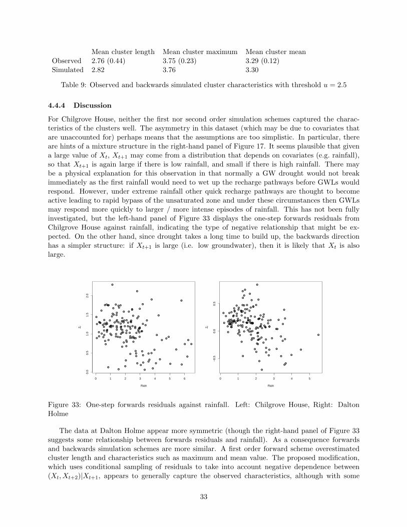
Mean cluster length Mean cluster maximum Mean cluster meanObserved 2.76 (0.44) 3.75 (0.23) 3.29 (0.12)Simulated 2.82 3.76 3.30

Table 9: Observed and backwards simulated cluster characteristics with threshold u = 2.5

4.4.4 Discussion

For Chilgrove House, neither the first nor second order simulation schemes captured the charac-teristics of the clusters well. The asymmetry in this dataset (which may be due to covariates thatare unaccounted for) perhaps means that the assumptions are too simplistic. In particular, thereare hints of a mixture structure in the right-hand panel of Figure 17. It seems plausible that givena large value of Xt, Xt+1 may come from a distribution that depends on covariates (e.g. rainfall),so that Xt+1 is again large if there is low rainfall, and small if there is high rainfall. There maybe a physical explanation for this observation in that normally a GW drought would not breakimmediately as the first rainfall would need to wet up the recharge pathways before GWLs wouldrespond. However, under extreme rainfall other quick recharge pathways are thought to becomeactive leading to rapid bypass of the unsaturated zone and under these circumstances then GWLsmay respond more quickly to larger / more intense episodes of rainfall. This has not been fullyinvestigated, but the left-hand panel of Figure 33 displays the one-step forwards residuals fromChilgrove House against rainfall, indicating the type of negative relationship that might be ex-pected. On the other hand, since drought takes a long time to build up, the backwards directionhas a simpler structure: if Xt+1 is large (i.e. low groundwater), then it is likely that Xt is alsolarge.

●

●

●

●

●

●

●

●

●

●

●

●

●●

●

●

●●

●

●

●●

●

●

●

●●

●

●

●

●

●●

●

●

●

●●

●

●

●

●

●

●

●

●

●

●

●

●

●

●

●

●

●

●

●

●

●

●

●

●

●

●

●

●

●

●

●

●

●

●

●

●

●

●

●

●

●

●

●

●

●

●

●

●●●

●

●

●

●

●

●

●

●

●

●

●

●

●

● ●

●

●

●

●

●

●

●

●

●

●

●

●

●

●

●

●

●●

●●

●

●

●●

●

●

●

●

●

●●

●

●

●

●

●

●●

●

●

●

●●

●

●

●

●

●

●

●

●●

● ●

●

●

●

0 1 2 3 4 5 6

0.0

0.5

1.0

1.5

2.0

Rain

Zf

●

●

●

●

●

●

● ●

●

●

●

●

●

●

●

●

●

●

●

●

●

●

● ●

●

●

●

●

●

●

● ●

●●●

●

●

●

●

●

●

●

●

●

●

●

●

●

●

●

●

●

●

●

●

●

●

●

●

●

●

●

● ●

●

●

●

●

●

●

●

●

●

●

●

●

●

●

●

●●

●

●

●

●

●

●

●●

●

●

●

●

●

●●

●●

●

●

●

●●

●

●

●

●

●

●

●

●

●

●

●

●

●

●

●

●

●

●

●

●

●

●●

●

●

●

●

●

●

●●

●

●

●

●

●

●

●

●

●

●

●

●

●

●

●

●●

●

●

●

●

●●

●

●

●

0 1 2 3 4 5

−0.

50.

00.

5

Rain

Zf

Figure 33: One-step forwards residuals against rainfall. Left: Chilgrove House, Right: DaltonHolme

The data at Dalton Holme appear more symmetric (though the right-hand panel of Figure 33suggests some relationship between forwards residuals and rainfall). As a consequence forwardsand backwards simulation schemes are more similar. A first order forward scheme overestimatedcluster length and characteristics such as maximum and mean value. The proposed modification,which uses conditional sampling of residuals to take into account negative dependence between(Xt, Xt+2)|Xt+1, appears to generally capture the observed characteristics, although with some

33

small overestimation remaining.

4.5 Case Study Summary

Through the course of this case study LU have demonstrated a number of extreme value theorymethodologies that are applicable to the study of extreme GWL and other phenomena that are ofinterest to BGS such as volcanoes, space weather events and soil contamination. These method-ologies can be used to predict the likelihood of the occurrence and severity of extreme events asa function of available covariates. Thus, in the case of GWL extremes it is possible to comparethe current frequency of extremes with the frequency that might occur according to future climatescenarios. Other models can be used to simulate successive extreme GWLs and to determine prop-erties of a multi-month extreme events. These models are more flexible and generally applicablethat the methodologies currently used by groundwater scientists when considering groundwaterextremes. The application of these models does require assumptions about the variable of interestbut LU have demonstrated strategies that might be used to relax these assumptions when they areinappropriate. The methodologies applied are analogous to the methods currently used by BGSin that the GWLs are standardised and deviations from the seasonal norm can be identified interms of thresholds on these standardized variables. However, these extreme value theory tech-niques acknowledge the potential for different behaviours in the tails of the distribution. BGS arenow applying these methodologies to a wider set of GWL data and in collaboration with LU willproduce a paper assessing the potential to use extreme value theory methodologies to characteriseextreme groundwater events.

4.6 References

Adams B., Bloomfield J.P., Gallagher A.J., Jackson C.R., Rutter H.K., Williams A.T. 2010. Anearly warning system for groundwater flooding in the Chalk. Q. Journal Eng. Geol. andHydrol., 43, 185-193

Bloomfield J.P., Marchant B.P., 2013. Analysis of groundwater drought using a variant of theStandardised Precipitation Index. Hydrology and Earth Systems Science, 17, 4769—4787.

Eltahir, E.A.B., Yeh, P. J-F., 1999. On the asymmetric response of aquifer water level to floodsand droughts in Illinois, Water Resources Research, 35, 1199-1217.

Heffernan, J.E., Tawn, J.A., 2004. A conditional approach for multivariate extreme values. Jour-nal of the Royal Statistical Society, B, 66, 497–546.

Ledford, A.W., Tawn, J.A., 1996. Statistics for near independence in multivariate extreme values.Biometrika, 83, 169–187.

Mackay, J.D., Jackson, C.R., Wang, L., 2014. A lumped conceptual model to simulate groundwaterlevel time-series. Environmental Modelling and Software, 61, 229—245.

McKee T.B., Doesken N.J., Kleist J. 1993. The Relationship of Drought Frequency and Durationto Time Scales. Proceedings of the Eighth Conference on Applied Climatology. AmericanMeteorological Society: Boston; 179-–184.

Monteith J.L., Unsworth M.H. 2008. Principles of Environmental Physics: Third Edition. Else-vier, London, UK.

34

Smith, R.L., Weissman, I., 1994. Estimating the extremal index. Journal of the Royal StatisticalSociety B, 56, 515–528.

Wilby, R.L., Noone, S., Murphy, C., Matthews, T.K.R., Harrigan, S., Broderick, C., 2016. Anevaluation of persistent meteorological drought using a homogeneous Island of Ireland pre-cipitation network. International Journal of Climatology, 36, 2854–2865.

Winter, H.C., Tawn, J.A., 2016. Modelling heatwaves in central France: a case study in extremaldependence. Journal of the Royal Statistical Society, C.

5 Appendix: MSc Project Proposals

5.1 The influence of soil texture on the potential for carbon sequestration

Numerous statistical challenges arise when mapping of soils, especially when assessing large areasand several properties that are driven by numerous controlling factors of various origins and scales.The objective of this study will focus on the development of a statistical framework to map togethera set of soil properties in a 3 dimensions geographical space. Most of the studies based their mapson a model for one depth and for a single property. This may produce inconsistent predictions ofthe set of variable at a given depth. For example, clay is one of the driving factors of organic carbon.Both are major input parameters of climate or agronomic models. They should then be predictedtogether The study area will be the ”Centre” region of France corresponding approximately tothe middle Loire catchment) and has a surface area of about 39472 km2. Two datasets will beused. The first soil dataset A consists of 2487 soil profiles of the French soil database (IGCS -Inventory Management and Soil Conservation) coming from the historical soil database and fromthe campaign related to the realization of the regional 1:250k soil map. The second dataset B isextracted from the database coming from the French soil monitoring network (Reseau de Mesuresde la Qualite des Sols: RMQS) (Jolivet et al., 2006) which is based on a systematic random grid(16 km x 16 km). The raw observations correspond to measurements realized on samples comingfrom soil horizons. The depths vary between sites. The modelling procedure will focus on a setof 4 soil properties: particle size (sand, silt, clay) and carbon. Additive-log-ratio (alr) transformwill have to be applied to particle size data in order to keep the compositional constraint thoroughthe modelling procedure. We will use auxiliary environmental covariate such as digital elevationmodel or geological maps in the framework of the linear mixed model. Dataset A will be used asa calibration dataset and dataset B as a validation dataset. The predictions will be produced perdepth increments that are the same at each prediction sites

5.2 Inter-relationships between rainfall, river level and ground water level

Groundwater level is a measure of the amount of water in storage within an aquifer. Understandinghow groundwater levels fluctuate over time is important as abstraction of this water is often re-quired, e.g. to supplement reservoir supplies in times of drought. Scientists at the British GeologicalSurvey (BGS) have available high-frequency data on groundwater levels (every minute), river levels(every minute) and rainfall (every 15 minutes) for a site in Wallingford, Oxfordshire. The goal ofthis project will be to understand the key drivers behind fluctuations in the groundwater level atthis site. Whilst it is clear that the groundwater level will be driven by both rainfall and riverlevel, it is much less clear what the most informative lag time will be to relate these two processesto the groundwater level. Further this lag will probably differ between river level and rainfall. Toinvestigate this, you will use exploratory data analysis to tease out the scale dependencies amongst

35

these three, highly related, series. You will then look at how this information can be incorporatedinto either a regression or multivariate model in order to fully quantify the relationships identified.

5.3 Extreme Space Weather

This project will be based on previous work by Alan Thompson and co-authors, who posed thequestion ’How extreme can geomagnetic storms become’? Geomagnetic storms have the potential toimpact on the UK power grid, aviation, satellite operations, GPS and communications and thereforethe UK government are interested in quantifying the 1-in-100 and 1-in-200 year extreme events forsuch storms. Geomagnetic time-series data is available for 28 European observatories. The datais very high frequency (1-minute) and so some declustering is required prior to the application ofa peaks over threshold extreme value model. Existing work on this data has modelled the dataacross sites separately, and has also ignored any non-stationary features in the data. Your core aimwill be to investigate any patterns and trends that may be observable within the extreme events,be these trends in space or time. Initially you will conduct a thorough exploratory data analysis,and then use the results of this to construct an appropriate temporal, or spatial, model.

36

STAGE: STAtistical modelling of Groundwater Extremes · STAGE: STAtistical modelling of Groundwater...

Documents

Transcript of STAGE: STAtistical modelling of Groundwater Extremes · STAGE: STAtistical modelling of Groundwater...