Stabilization in spite of matched unmodelled dynamics

and

An equivalent definition of input-to-state stability

Laurent PralyCentre Automatique et Systemes

Ecole des Mines de Paris35 rue St Honore

77305 Fontainebleau cedexFRANCE

praly@cas.ensmp.fr

Yuan Wang∗

Department of MathematicsFlorida Atlantic University

777 Glades RoadBoca Raton, FL 33431

USA

ywang@polya.math.fau.edu

Abstract. We consider nonlinear systems with input-to-output stable (IOS) unmodelled dynamicswhich are in the “range” of the input. Assuming the nominal system is globally asymptoticallystabilizable and a nonlinear small gain condition is satisfied, we propose a first control law such thatall solutions of the perturbed system are bounded and the state of the nominal system is capturedby an arbitrarily small neighborhood of the origin. The design of this controller is based on again assignment result which allows us to prove our statement via a Small-Gain Theorem [JTP,Theorem 2.1]. However, this control law exhibits a high gain feature for all values. Since this maybe undesirable, in a second stage we propose another controller with different characteristics in thisrespect. This controller requires more a priori knowledge on the unmodelled dynamics, as it isdynamic and incorporates a signal bounding the unmodelled effects. However this is only possibleby restraining the IOS property into the exp-IOS property. Nevertheless we show that, in the case ofinput-to-state stability (ISS) — the output is the state itself —, ISS and exp-ISS are in fact equivalentproperties.

Key Words. Nonlinear systems, Robust control, Uncertain systems, Gain assignment, Input-to-state stability.

∗Supported in part by NSF Grant DMS-9403924 and by a scholarship from Universite Lyon I, France.

Submitted for publication in Mathematics of Control, Signals and SystemsFirst submission : September 30, 1994, Revision : January 29, 1996

1

1 Introduction

Consider the system : x = f(x) +

p∑i=1

gi(x) [ui + ci(x, z, u)]

z = a(x, z, u)

(1)

where a and f are continuous vector fields, G = (gi) is a continuous “matrix field”, and c1, . . . , cp

are continuous functions. The x-subsystem represents, when c = 0, the nominal system. Its statex, taking values in IRn, is measured and the vector u = (ui), taking values in IRp, is its input. Thez-subsystem represents the unmodelled dynamics, its state z, taking values in IRm, is unmeasuredand the functions a and c are unknown.

The problem is to design a feedback law, with x as only input, guaranteeing boundedness of thesolutions of the closed-loop system and regulating x around 0. To solve this problem we shall assume(see A1) that the nominal system is globally asymptotically stabilizable and that the z-subsystemhas an appropriately “stable” input-output behavior (see A2 or A2’).

In the terminology of linear systems, the perturbation introduced via c would be called stableand proper multiplicative perturbation. Its main characteristics are :– The relative degree between u and any “generic” output function of x cannot be decreased by the

presence of c.– The so called matching assumption is met. Namely, if c were measured, we could completely

annihilate its effects on the x-subsystem (see [I, Remark 4.6.2]). Here c is not assumed to bemeasured. Instead, we shall impose an amplitude limitation (see A2 or A2’).

– The state x can be measured, and consequently, there is no inverse dynamics. This makes ittheoretically possible to use “high gain” controllers. However, we know that, if other classesof “real life” unmodelled effects – input saturations, unmeasured noise, unmatched unmodelleddynamics, . . . – are present, then “high gain” controllers may be unsuitable. For this reason, weshall propose two solutions to the problem stated above with a different high gain requirement.The topic of stabilizing (nonlinear) systems with uncertainties has been attracting the attention

of many authors for a long time, see for instance [BCL, C, CL, G, K]. While most of the workin this area focused on unmodelled static (time varying) uncertainties, less work has been donefor systems with dynamic uncertainties. The recent work [KSK] has formulated very properly theproblem of stabilizability for nonlinear systems with unmodelled dynamics. There also, the authorshave proposed a solution for a specific class of systems with linear unmodelled dynamics at the input.Some related work in this area can also be found in [Q1, Q2], where the author has investigated thetracking problem for linear systems with unmodelled dynamic uncertainties.

Our problem generalizes the one stated and solved by Krstic, Sun and Kokotovic in [KSK, Lemma3.1] for x in IR and functions c and a linear and not depending on x. The solution proposed by theseauthors incorporates, in the controller, a signal, called normalizing signal which captures the effectof the unmodelled dynamics. This concept of normalizing signal is nowadays widely used in linearadaptive control, and its extension to the nonlinear case has been suggested in [JP1, JP2, J]. Jiang,Mareels and Pomet have shown in [JMP] that the result of [KSK, Lemma 3.1] holds also with a staticfeedback law, without using the normalizing signal. For this, an appropriate change of coordinatesof the unmodelled dynamics is made and the technique of propagating the ISS property through

2

integrators proposed in [JTP] is applied. Based on the technique of gain assignment and the Small-Gain Theorem of [JTP], Krstic and Kokotovic have obtained another solution in [KK], withoutnormalizing signal for the system (1), allowing the functions c and a to be nonlinear and to dependon x but still imposing that x be in IR.

Here, we extend the work in [KK] to the general case when x is in IRn. Our major assumptions are:(1) the nominal system is stabilizable, and (2) the unmodelled dynamics is input-to-output stable(IOS) with a small enough gain function. In the special case when there is no dynamic uncertaintypresented in the system, that is, when the functions ci’s do not depend on z, the IOS condition reducesto the usual boundedness condition on the static uncertainties considered, for instance, in [C, K, Q2].After stating our assumptions in section 2, we shall propose, in section 3, a first control law whichsolves the problem. It is a static feedback but, as already mentioned, it exhibits a high gain feature.This feature has been found usefull to solve some problems in robust control (see for instance [BCL]and [SK]) but it may also be undesirable in some other situations. This motivates our proposition of asecond controller in section 4. Our two controllers are compared for a simplistic example in section 5.In section 6 we propose a framework allowing us to relax somehow the assumptions made in section 2.In fact, to prove that our second controller provides the closed-loop system with properties similar tothe ones given by the first one, we need to restrain the class of unmodelled dynamics. Neverthelessin the case ci(x, z, u) = z, i.e. the disturbance is the state of the unmodelled dynamics itself, weprove in section 7 that there is in fact no restriction.

2 Assumptions

We assume the nominal system is globally asymptotically stabilizable and more precisely :

A1 : We know a C1 positive definite function V satisfying, for all x,

V (x) ≥ α1(|x|) , (2)

for some function α1 of class1 K∞, and a C0 feedback law un(x) with un(0) = 02, such thatthe function3 :

W (x) = −L[f+Gun]V (x) (3)

is also positive definite.

According to [S1], if there exists un satisfying Assumption A1, then the following feedback us

also globally asymptotically stabilizes the nominal system :

usi(x) =

−LfV (x) +

√LfV (x)2 + ‖LGV (x)‖4

‖LGV (x)‖2LgiV (x) , if LGV (x) 6= 0 ,

0 , if LGV (x) = 0 ,

(4)

1For the definitions of class K, K∞ and KL functions see [H].2Assuming un(0) = 0 can be done without loss of generality as far the nominal system is concerned. Indeed, if

un(0) = u0 6= 0, it is sufficient to replace f by f = f + Gu0 and u by u = u− u0.3LfV is the Lie derivative of V along f and LGV is the row vector (LgiV ).

3

where ‖·‖ denotes the usual Euclidian norm of IRp. With this control we get the following positivedefinite function :

Ws(x) = −L[f+Gus]V (x) . (5)

The interest of this particular feedback is that we have, for all x,

LGV (x) 6= 0 =⇒ LGV (x)us(x) < 0 . (6)

A2 : The z-subsystem of (1) with input (x, u) and output c is BIBS and IOpS. That is:

BIBS : For each initial condition z(0) and each measurable essentially bounded function (x, u) :IR≥0 → IRn × IRp, the corresponding solution z(t) is defined and bounded on IR≥0.

IOpS : There exist a function βc of class KL, two functions γu and γx of class K and a posi-tive real number c0 such that, for each initial condition z(0) and each measurable essentiallybounded function (x, u) : IR≥0 → IRn × IRp, the corresponding solution satisfies, for all t inIR≥0,4

|c(t)| ≤ c0 + βc(|z(0)|, t) + γu(U(t)) + γx( supτ∈[0,t)

{|x(τ)|}) , (7)

where :U(t) = sup

τ∈[0,t){|u(τ)|} , (8)

and for each vector v in IRp, |v| denotes max{|v1|, . . . , |vp|}, and similarly for vectors in IRn.

With Assumption A2, we shall be able to get a control law whose design is based on the onlyfact that inequality (7) holds. However Krstic and Kokotovic have noticed in [KK] that betterperformance can be obtained if one uses more a priori knowledge on c, namely that the last twoterms in the right hand side of (7) can be evaluated on line and therefore used in the control law.Unfortunately such terms involve U which is the output of an infinite dimensional system with uas input. To overcome this difficulty, we remark that assumption A2 could apply to systems withdynamics involving mathematical objects more complex than the system :{

z = a(x, z, u) ,y = c(x, z, u) .

(9)

In particular, when the initial condition z(0) is fixed, this system provides operators: u 7→ z andu 7→ y which are finite dimensional, the former being strictly proper, whereas, in (8), the operator:u 7→ U is only proper and infinite dimensional. From this, we conjecture that the restriction of A2to systems in the particular form (9) should give a stronger property. These arguments lead us torestrain assumption A2 with replacing the infinite dimensional operator supτ∈[0,t) {·} by a first orderone. This yields :

A2’ The z-subsystem with input u and output c is BIBS and exp-IOpS. That is:

exp-IOpS : For some positive real number µ and some functions γvx, γvu, γcx and γc of class

4For the sake of simplicity, here and all along the paper we make the following abuse of notations: sup is to be takenas the essential supremum norm and “for all t” should be “for almost all t with respect to the Lebesgue measure”.

4

K, there exist a positive real number co, a function γcu of class K and a function β of class KL,such that, for each initial condition z(0) and for each measurable essentially bounded function(x, u) : IR≥0 → IRn × IRp, the corresponding solution satisfies, for all t in IR≥0,

|c(t)| ≤ c0 + β(|z(0)|, t) + γcu(|u(t)|) + γcx(|x(t)|) + γc(r(t)) , (10)

where the function r(t) satisfies the following equations :

r = −µ r + γvu(|u|) + γvx(|x|) , r(0) = 0 . (11)

The main difference between IOpS and exp-IOpS is that in (10), through r, an exponentially weightedL1 norm is used instead of the L∞ one expressed in U . Clearly, exp-IOpS implies IOpS with thegains of the relations u 7→ c and x 7→ c given by :

γu = γcu + γc ◦ 1µ γvu , γx = γcx + γc ◦ 1

µ γvx (12)

respectively. But the previous arguments let us expect that the converse may be true. This will beproved in section 7 for the case when c = z.

Assumption A2’ is strongly related with Assumption UEC (73) in [JP1]. From this relation, wenote :– [JP1, Lemma 1] is a helpful tool for selecting the real number µ and the functions γvx, γvu, γcx

and γc.– Equations in (11) provide us with r as a pseudo state for the stability analysis. In the proof of [JP1,

Proposition 1], it is shown that it is well suited for the application of Lyapunov second method.– To help the reader get a better grip on the meaning of this signal r, we refer to [P, Property 1].

Let us remark that Assumption A1 and A2 or A2’ are not sufficient for guaranteeing the existenceof a feedback law solving our problem. Consider the system : x = x2 − (u− γ(z))x ,

z = (u− z) z2 ,(13)

where γ is a smooth odd function satisfying :

sign(r) [r − γ(r)] ≤ M ∀ r ∈ IR , (14)

for some positive real number M . This condition says roughly that the function γ grows at least asmuch as the identity function. Assumption A1 holds, with :

V (x) = 12 x2 , un(x) = x + x2 , (15)

and Assumption A2 holds also since the z-subsystem with input u and output γ(z) is IOS withγx ≡ 0 and γu, any gain function of class K strictly greater than γ. However system (13) is notasymptotically controllable. Precisely, we prove in Appendix A that there is no control law u(t) thatcan drive to zero the x-component of any solution starting from (x0, 1) with x0 > M exp(1).

This example shows that it is in general impossible to solve the problem stated in section 1 if thefunction Id− γu is bounded.

5

3 First solution with a static feedback

Proposition 1 Assume A1 and A2 hold. Under this condition, for any functions κu and κx of classK∞, there exists a continuous feedback law ω(x) such that all the solutions of the closed-loop system(1) are bounded provided that we have :

(Id + ρ2) ◦ [γu ◦ (Id + ρ1) ◦ (Id + κu) + γx ◦ (Id + ρ1) ◦ κx] ≤ Id (16)

for some functions ρ1 and ρ2 of class K∞. Moreover, for each closed-loop solution, we have :

lim supt→+∞

|x(t)| ≤ κx ◦ (Id + ρ−12 )(c0) . (17)

Remark 2 : If, in (7), c0 = 0, that is, when the z-subsystem of (1) is IOS with (x, u) as input andc as output, then it follows immediately from (17) that :

limt→+∞

|x(t)| = 0 . (18)

If c0 6= 0, since κx can be chosen as an arbitrarily small function of class K∞, (16) is mainly acondition on γu and (17) gives a practical convergence result. In fact, it can be shown that, for anygiven functions γu and γx of class K, satisfying :

Id− γu > ρ0 , (19)

for some function ρ0 of class K∞, we can find functions ρ1, ρ2, κu and κx of class K∞ such that (16)holds. Note also that we do not claim stability in the proposition.

Proposition 1 will be established by showing first the existence of a continuous feedback law ω(x)assigning appropriate gains to the system :

x = f(x) + G(x) [ω(x) + c] (20)

with c as input and (x, ω(x)) as output. The conclusion will then follow from the Small-Gain Theorem[JTP, Theorem 2.1].

Lemma 3 (Strong Gain Assignment Theorem) Assume A1 holds. Then for any functions κu

and κx of class K∞, there exists a continuous feedback law ω(x) and functions βu and βx of classKL, such that, for each initial condition x(0) and for each measurable essentially bounded functionc : IR≥0 → IRp, the corresponding solutions of :

x = f(x) + G(x) [ω(x) + c(t)] (21)

satisfy, for all 0 ≤ s ≤ t,

|ω(x(t))| ≤ βu(|x(s)|, t− s) + (Id + κu)

(sup

τ∈[s,t){|c(τ)|}

), (22)

|x(t)| ≤ βx(|x(s)|, t− s) + κx

(sup

τ∈[s,t){|c(τ)|}

). (23)

6

This result is to be compared with [JTP, Theorem 2.2]. We have here a stronger statement sincenot only any gain can be assigned to the relation c 7→ x but also we can limit the gain of the relationc 7→ ω.

Proof of Lemma 3. Let V and α1 be the functions as in Assumption A1, and let V(21) denote thefunction :

V(21)(x, t) =∂V

∂x(x) (f(x) + G(x) [ω(x) + c(t)]) . (24)

With assumption A1, we have :

V(21)(x, t) ≤ −W (x) + LGV (x)ω(x)− LGV (x)un(x) + LGV (x)c(t) . (25)

We restrict our attention to feedback laws ω of the form :

ωi(x) = −sign(LgiV (x)) ωi(x), ωi(x) ≥ 0 , i = 1, 2, . . . , p, (26)

where the functions ωi will be defined below. This yields :

V(21)(x, t) ≤ −W (x) −p∑

i=1

|LgiV (x)|(ωi(x) − |uni(x)| − |c(t)|

). (27)

To define ωi, we let S be a function of class K∞ such that, for all s and x, we have :

κ−1u (|un(x)|) ≤ S(V (x)) , κ−1

x ◦ α−11 (s) ≤ S(s) . (28)

Such a function exists since V is positive definite and proper. Then we choose ωi as :

ωi(x) = θi(x) bi(x) , (29)

where :bi(x) = |uni(x)| + S(V (x)) (30)

and θi is a function introduced to enforce continuity and defined as follows :For each i, let :

B0i = {x : LgiV (x) = 0, x 6= 0} , (31)

and :B1i =

{x : |LgiV (x)|

(S(V (x)) + |uni(x)|

)≥ W (x)

2p, x 6= 0

}. (32)

Since W is positive definite, B0i and B1i are closed and disjoint subsets of IRn \{0}. It follows that wecan define this function θi : IRn \ {0} → [0, 1] as a continuous function satisfying (see the appendixfor an explicit expression of such a function) :

θi(x) =

{1 , if x ∈ B1i ,

0 , if x ∈ B0i .(33)

7

To get a definition of θi on IRn we simply add θi(0) = 0. Then, though θi may fail to be continuousat 0, the function ω is continuous on IRn since bi(0) = 0. Hence, from (27), we get:

V(21)(x, t) ≤ −W (x) −p∑

i=1

|LgiV (x)| [θi(x) (S(V (x)) + |uni(x)|)− |uni(x)| − |c(t)|]

≤ −W (x) +p∑

i=1

|LgiV (x)| (1− θi(x)) (S(V (x)) + |uni(x)|)

−( p∑

i=1

|LgiV (x)|)

(S(V (x))− |c(t)|)

≤ −W (x)2

−( p∑

i=1

|LgiV (x)|)

(S(V (x))− |c(t)|) . (34)

From this latter inequality, by using the fact that W is positive definite, V and S are positive definiteand proper and following the same lines as in the Claims on p. 441 in [S2], we can show the existenceof a function βv of class KL such that, for all 0 ≤ s ≤ t, we have :

V (x(t)) ≤ max

{βv(V (x(s)), t− s) , S−1

(sup

τ∈[s,t){|c(τ)}|

)}. (35)

Inequality (23) follows readily with (28) and (2). Then, since we have :

|ω(x)| ≤ (Id + κu) ◦ S(V (x)) , (36)

the conclusion follows.

Remark 4 : If instead of using un, we use us satisfying (6), the control law ω can be made simplerby modifying (29) and (30) so that :

ωi(x) = usi(x) − θi(x) sign(LgiV (x))S(V (x)) , (37)

and B1i in (32) into :

B1i ={

x : |LgiV (x)| S(V (x)) ≥ Ws(x)2p

, x 6= 0}

. (38)

Remark 5 : The control law ω can be made smooth if one allows the addition of arbitrarily smallpositive numbers to the right hand side of (22) and (23) (see [JTP]). More specifically, for any ε0 > 0,one can always approximate each ωi(x) by a smooth function ωi(x) so that, for all x ∈ IRn, we have :

|ωi(x)− ωi(x)| < ε0 . (39)

But, with such a choice of ωi, it may fail to hold that :

LgiV (x) ωi(x) ≤ 0, ∀x ∈ IRn . (40)

8

To get a smooth feedback ωi satisfying restriction (40), we proceed as follows :For each m ∈ {1, . . . ,m}, we let B2i denote the open subset of IRn where ωi(x) 6= 0. We define :

σi(x) = min{ |ωi(x)|

2,

ε0

2

}. (41)

so that σi(x) > 0 for all x ∈ B2i. Hence, there exists a function ωi(x) that is smooth on B2i and suchthat :

|ωi(x)− ωi(x)| < σi(x) (42)

for all x ∈ B2i (cf. [B, Theorem 4.8, p197]). One can then extends of the domain of ωi to IRn byletting ωi(x) = 0 for x 6∈ B2i. Note then that ωi(x) is continuous everywhere, and, for all x ∈ IRn,

ωi(x) ωi(x) ≥ 0 . (43)

Now we let θi(x) : IRn → [0, 1] be a smooth function satisfying the following :

θi(x) =

{0 , if x ∈ B3i ,

1 , if x ∈ B4i ,(44)

where the two sets B3i and B4i are defined by :

B3i = {x ∈ IRn : |ωi(x)| ≤ ε0/4} , B4i = {x ∈ IRn : |ωi(x)| ≥ ε0/2} . (45)

As before, such a smooth funciton exists because B3i and B4i are two disjoint closed subsets of IRn.Finally we let :

ωi(x) = θi(x) ωi(x) . (46)

Then ωi is smooth everywhere, and, for all x ∈ IRn,

ωi(x) LgiV (x) ≤ 0 , |ωi(x)− ωi(x)| < ε0 . (47)

Consequently, when the controls ωi’s are used instead of the ωi’s, (34) becomes :

V(21)(x, t) ≤ −W (x)2

−( p∑

i=1

|LgiV (x)|)

(S(V (x))− |c(t)| − ε0) . (48)

It follows that (22) and (23) are replaced by :

|ω(x(t))| ≤ βu(|x(s)|, t− s) + (Id + κu)

(sup

τ∈[s,t){c(τ)}+ ε0

)+ pε0

≤ βu(|x(s)|, t− s) + (Id + κu)

(sup

τ∈[s,t){c(τ)}

)(49)

|x(t)| ≤ βx(|x(s)|, t− s) + κx

(sup

τ∈[s,t){c(τ)}

), (50)

where c = |c|+ (p + 1)ε0.

9

Proof of Proposition 1. By applying Lemma 3 we get a continuous feedback law ω(x) which, whenapplied to (1), gives a closed-loop system which can be seen as the interconnection :

x = f(x) + g(x) [ω(x) + y1] , y1 = c(x, z, ω(x)) , (51)

z = a(y21, z, y22) , y21 = x , y22 = ω(x) , (52)

where, from (7), (22) and (23),

|y1(t)| ≤ c0 + βc(|z(0)|, t) + γu

(sup

τ∈[0,t){|y22(τ)|}

)+ γx

(sup

τ∈[0,t){|y21(τ)|}

), (53)

|y22(t)| ≤ βu(|x(0)|, t) + (Id + κu)

(sup

τ∈[0,t){|y1(τ)|}

), (54)

|y21(t)| ≤ βx(|x(0)|, t) + κx

(sup

τ∈[0,t){|y1(τ)|}

). (55)

To conclude we could apply [JTP, Theorem 2.1] if :– the function ω(x) were locally Lipschitz,– we would have a one channel interconnection instead of the two channels given by y21 and y22 ,Nevertheless, if the statement of this Theorem is not exactly appropriate, we can follow line by lineits proof. First we can show with (16) that the outputs corresponding to any solutions are boundedon their maximal interval of definition. In particular, we have (see [JTP, (80)]) :

|y1(t)| ≤ c0 + βc(|z(0)|, t) + γu

(βu(|x(0)|, 0) + (Id + κu)

(sup

τ∈[0,t){|y1(τ)|}

))

+ γx

(βx(|x(0)|, 0) + κx

(sup

τ∈[0,t){|c(τ)|}

)). (56)

With (16), this yields (see [JTP, (83)]) :

supτ∈[0,t)

{|y1(τ)|} ≤ (Id + ρ−12 )(

βc

(|z(0)|, 0

)+ γu ◦ (Id + ρ−1

1 )(βu(|x(0)|, 0)

)

+ γx ◦ (Id + ρ−11 )(βx(|x(0)|, 0)

)+ c0

). (57)

With the BIBS property of both subsystems, this implies that all the solutions are defined andbounded on IR≥0. This means that, for each (x(t), z(t)), there exists a positive real number s∞ sothat, for all t in IR≥0, we have :

|(x(t), z(t))| ≤ s∞ . (58)

Second, we get, for all t in IR≥0 (see [JTP, (93)]),

|y1(t)| ≤[βc(s∞, t/2) + γu ◦ (Id + ρ−1

1 ) ◦ βu(s∞, t/4) + γx ◦ (Id + ρ−11 ) ◦ βx(s∞, t/4)

]+ (Id + ρ2)−1

(sup

τ∈[t/4,∞){|y1(τ)|}

)+ c0 . (59)

10

So, with [JTP, Lemma A.1], for any function ρ3 of class K∞, we know the existence of a function βof class KL such that we have, for all t in IR≥0,

|y1(t)| ≤ β(s∞, t) + (Id + ρ−12 ) ◦ (Id + ρ3)(c0) . (60)

Since, with (58) and (52), (23) gives :

|x(t)| ≤ βx(s∞, t/2) + κx

(sup

τ∈[t/2,∞){|y1(τ)|}

), (61)

It follows readily that :

lim supt→∞

|x(t)| ≤ κx ◦ (Id + ρ−12 ) ◦ (Id + ρ3)(c0) , (62)

for any function ρ3 of class K∞. But the solution (x(t), z(t)) is independent of ρ3, this implies (17). 2

4 Second solution with a dynamic feedback

The solution we have proposed in the previous section relies on the use of high gain. This fact ishidden in the choice of the function S which has to be sufficiently large and not only for small values.This may lead to problems if other robustness problems are considered. What is leading to high gainin the previous approach is the use of the matching assumption and a worst case design. By usingmore a priori knowledge on the unmodelled dynamics one may hope high gain to be involved in adifferent way. To this purpose, we incorporate assumption A2’ in the following result.

Proposition 6 Assume A1 holds with W a proper function5, i.e. precisely :

α3(V (x)) ≤ 12 W (x) , (63)

where α3 is some function of class K∞ . Let us choose a real number µ, functions γvu and γc ofclass K and a function κ1 of class K∞ so that :

γvu ◦ (Id + ρ4) ◦ κ−11 ◦ (Id + ρ4) ◦ γc ≤ µ Id − ρ5 (64)

for some functions ρ4 and ρ5 of class K∞. We assume that, with such a choice, Assumption A2’holds with a function γcu satisfying :

γcu ≤ Id− κ1 . (65)

Under these conditions, for any functions κ2, κ3 and κ4 of class K∞, there exists a continuousdynamic feedback law ω(x, r) with r given by (11) such that all the solutions of the closed-loopsystem are bounded and their x-components satisfy :

lim supt→+∞

|x(t)| ≤ α−11 ◦ (Id + κ−1

3 ) ◦ α−13 ◦ (Id + κ−1

4 ) (c0κ2(c0)) . (66)

5With Assumption A1, we can always modify the function V to meet this requirement (see Proposition 13 forinstance).

11

Remark 7 : When c0 = 0, we get convergence of the x-component :

limt→+∞

|x(t)| = 0 . (67)

When c0 6= 0, since κ2, κ−13 and κ−1

4 can be chosen as arbitrarily small functions of class K∞, (66)gives a practical convergence result.

Proof. First, we remark, with (11), that r(t) is nonnegative for any t in IR≥0. Then, we follow thesame lines as for the proof of Lemma 3. Let V(1) denote the function :

V(1)(x, u, t) =∂V

∂x(x)(f(x) + G(x)(u + c(t))

), (68)

and let ω be chosen of the form :

ωi = −sign(LgiV (x)) ωi , ωi ≥ 0 , i = 1, 2, . . . , p , (69)

with functions ωi to be defined below. With (10), we get :

V(1)(x, ω, t) ≤ −W (x) −p∑

i=1

|LgiV |(ωi − |uni(x)|

)

+p∑

i=1

|LgiV |(c0 + β(|z(0)|, t) + γcu(|ω|) + γcx(|x|) + γc(r)

). (70)

To define the functions ωi, let κ2 be the function of class K∞ chosen in Proposition 6. Let usalso choose a function ` of class K and bounded by `∞. Since, for any positive real numbers a, b, wehave :

ab ≤ κ2(b) b

p+ κ−1

2 (pa) a (71)

(consider two cases: a ≤ κ2(b)/p and a ≥ κ2(b)/p), we obtain :

V(1)(x, ω, t) ≤ −W (x) −p∑

i=1

|LgiV |(ωi − γcu(|ω|) − bi(x) − γc(r)

)+ v0(t)κ2(v0(t)) , (72)

where v0(t) is defined as :v0(t) = β(|z(0)|, t) + c0 , (73)

and, for each i,bi(x) = |uni(x)| + γcx(|x|) + κ−1

2 (p|LgiV (x)|) . (74)

Let :b(x) = max

j∈{1,...,p}

{bj(x)

}. (75)

We define ωi as :ωi(x, r) = θi(x, r) κ−1

1

(b(x) + γc(r)

), (76)

12

where κ1 is chosen in Proposition 6. As in (29), the function θi : IRn × IR → [0, 1] is introduced toenforce the continuity. It is defined as follows :For each i, let :

B0i = {(x, r) : LgiV (x) = 0, (x, r) 6= (0, 0)} , (77)

and :B1i =

{(x, r) : |LgiV (x)|κ−1

1 (b(x) + γc(r)) ≥W (x)

2p+

`(r)p

, (x, r) 6= (0, 0)}

. (78)

Since both W and ` are positive definite, it follows that B0i and B1i are disjoint closed subsets ofIRn × IR \ {(0, 0)}. Then, one can define a continuous function θi : IRn × IR \ {(0, 0)} → [0, 1] suchthat :

θi(x, r) =

{1 , if x ∈ B1i ,

0 , if x ∈ B0i .(79)

To get a definition of θi on IRn × IR we simply let θi(0, 0) = 0. Although θi may fail to be continuousat (0, 0), the functions ωi and ωi are continuous on IRn × IR since b(0) = γc(0) = 0.

Now, since condition (65) implies :

ωi(x, r)− γcu(|ω(x, r)|) ≥ (−(1− θi(x, r)) Id + Id − γcu) ◦ κ−11 (b(x) + γc(r))

≥ −(1− θi(x, r))κ−11

(b(x) + γc(r)

)+ b(x) + γc(r) , (80)

inequality (72) becomes, with (63), (76), (75) and the definition of θi,

V(1)(x, ω, t) ≤ −W (x) +p∑

i=1

|LgiV |(1− θi(x, r))κ−11 (b(x) + γc(r)) + v0(t)κ2(v0(t))

≤ −12 W (x) + v0(t)κ2(v0(t)) + `(r)

≤ −α3(V (x)) + v0(t)κ2(v0(t)) + `(r) . (81)

On the other hand, with the control law given by (76), the equations (11) imply :

r ≤ −µ r + γvu ◦ κ−11 (b(x) + γc(r)) + γvx(|x|) . (82)

With condition (64), it follows :

µ r − γvu◦ κ−11 (b(x) + γc(r)) ≥ µ r − γvu

(κ−1

1 ◦ (Id + ρ4) ◦ γc(r) + κ−11 ◦ (Id + ρ−1

4 )(b(x)))

≥ µ r − γvu ◦ (Id + ρ4) ◦ κ−11 ◦ (Id + ρ4) ◦ γc(r)

− γvu ◦ (Id + ρ−14 ) ◦ κ−1

1 ◦ (Id + ρ−14 )(b(x)))

≥ ρ5(r) − γvu ◦ (Id + ρ−14 ) ◦ κ−1

1 ◦ (Id + ρ−14 )(b(x)) . (83)

Let ρ6 be a function of class K∞ satisfying :

γvx(|x|) + γvu ◦ (Id + ρ−14 ) ◦ κ−1

1 ◦ (Id + ρ−14 )(b(x)) ≤ ρ6(V (x)) . (84)

13

Such a function exists since (2) holds for all x. With (81), we have finally obtained the followingsystem of differential inequalities :

V(1)(x, ω, t) ≤ −α3(V (x)) + v0(t)κ2(v0(t)) + `(r)

≤ −α3(V (x)) + v0(t)κ2(v0(t)) + `∞ ,

r ≤ −ρ5(r) + ρ6(V (x)) .

(85)

Now let (x(t), r(t), z(t)) be a solution of the closed-loop system (1),(11),(69),(76). Such a solutionexists for any initial condition (x(0), z(0)) and has a right maximal interval of definition [0, T ). Butsince α3 is of class K∞, V is proper, v0 and ` are bounded, (85) implies that x(t) is bounded on [0, T ).This, with the fact that ρ5 is of class K∞, implies that r(t) is also bounded on [0, T ). It follows thatthe control :

u(t) = ω(x(t), r(t)) (86)

is bounded on [0, T ). So with the BIBS property of the z subsystem, z(t) is bounded on [0, T ).Hence, by contradiction, one shows that the solution is defined and bounded on IR≥0, i.e., for all t inIR≥0,

‖(V (x(t)), r(t), z(t))‖ ≤ s∞ < +∞ . (87)

Also, as in the proof of Proposition 1, by following the same lines as in the Claims on p. 441in [S2], for any functions ρv and ρr of class K∞, with :

ρv ≤ Id , (88)

we can show the existence of class KL functions βv and βr such that, for all 0 ≤ s ≤ t, we have :

V (x(t)) ≤ βv(V (x(s)), t− s) + α−13 ◦ (Id + ρv)

(sup

τ∈[s,t){yr(τ)}

), (89)

r(t) ≤ βr(r(s), t− s) + ρ−15 ◦ 2ρ6

(sup

τ∈[s,t){V (x(τ))}

), (90)

where we have introduced the function :

yr(t) = v0(t)κ2(v0(t)) + `(r(t)) . (91)

But since :lim supt→+∞

yr(t) ≤ c0κ2(c0) + `∞ , (92)

by taking s = t/2 in (89) and using (87), we conclude readily that :

lim supt→∞

V (x(t)) ≤ α−13 ◦ (Id + ρv)(c0κ2(c0) + `∞) , (93)

The facts that function ρv is arbitrary and the solution (x(t), r(t), z(t)) is independent of ρv implythat

lim supt→∞

V (x(t)) ≤ α−13 (c0κ2(c0) + `∞) , (94)

14

from which it follows :lim supt→+∞

|x(t)| ≤ α−11 ◦ α−1

3 (c0κ2(c0) + `∞) . (95)

To show that this bound can be improved, we proceed as follows. Let us choose the function ` notonly of class K and bounded by `∞ but also satisfying :

` ≤ ρ7 , (96)

where ρ7 is of class K∞ and defined by :

ρ7 = (2(Id + κ4))−1 ◦ α3 ◦ (Id + κ3)

−1 ◦ (2ρ6)−1 ◦

(2ρ−1

5

)−1. (97)

The constraint (96) can always be satisfied and the function ρ7 depends only on known data. Indeed,– the functions κ3 and κ4 are chosen in Proposition 6,– the function α3 is obtained, in order to meet (63), from the known function V and W ,– the functions ρ4 and ρ5 are obtained, in order to meet (64), from the chosen quantities µ, γvu, γc

and κ1,– the function ρ6 is obtained, in order to meet (84), from the known or chosen functions γvu, ρ4, κ1,

un, γcx, κ2, g, γvx and V .Then, from (89), (91) and (90), we can consider the interconnection of a fictitious system with statex, input yr and output V (x) with a fictitious system with state r, input V (x) and output `(r).Although the systems are fictitious, the proof of the Small-Gain Theorem [JTP, Theorem 2.1] stillapplies. This can be seen by writing, in a way similar to (59),

V (x(t)) ≤ βv(s∞, t/2) + α−13 ◦ (Id + ρv) ◦ (Id + κ−1

4 ) (v0(t/2)κ2(v0(t/2)))

+ α−13 ◦ (Id + ρv) ◦ (Id + κ4) ◦ `(2βr(s∞, t/4))

+ α−13 ◦ (Id + ρv) ◦ (Id + κ4) ◦ ` ◦ 2ρ−1

5 ◦ 2ρ6

(sup

τ∈[t/4,+∞){V (x(τ))}

). (98)

So, with (88) and (96), we can again apply [JTP, Lemma A.1] to conclude that :

lim supt→∞

V (x(t)) ≤ (Id + κ−13 ) ◦ (Id + ρ8) ◦ α−1

3 ◦ (Id + ρv) ◦ (Id + κ−14 )(c0κ2(c0)) (99)

holds for any functions ρ8 and ρv of class K∞ with (88) satisfied. From this we get (66). 2

5 Comparison between the static and dynamic feedback designs

Two common features of the designs we have proposed are that they require a similar small gaincondition and, when c0 6= 0, they provide practical stability for the closed-loop system with a residualset which can be made smaller at the price of introducing a high gain feature for small values :

– Indeed, condition (16) of Proposition 1 and (64),(65) of Proposition 6 are approximately equivalent.In (16), since ρ1, ρ2 and κx are arbitrary, this condition can be interpreted as mainly requiringthat the function Id − γu be bounded below by a function of class K∞. Similarly in (64), since

15

ρ4 and ρ5 are arbitrary, this condition is mainly that the real number µ and the functions γvu, κ1

and γc should be chosen such that the function κ1 −(γcu ◦ 1

µ γvu

)is bounded below by a function

of class K∞. Then, (65) is mainly requiring that the function Id −(γcu + γc ◦ 1

µ γvu

)is bounded

below by a function of class K∞. Our remark follows with (12).

– Concerning the size of the residual set, in the static case, i.e. in the context of Proposition 1, thesolutions can be made to converge to a smaller neighborhood of the origin by choosing a smallerfunction κx. In the dynamic design, i.e. in the context of Proposition 6, one does so by choosinga smaller function κ2. In both cases, this causes the “high gain” phenomenon at least for smallvalues : in the static design, one needs to choose a bigger function S (see (28)), while in thedynamic design, the same problem occurs with the term κ−1

2 (p|LgiV (x)|) in (74).

Two significant differences between the designs are that the dynamic design requires more a prioriknowledge and that, when c0 is known to be 0 and the unmodelled effect is more dynamic, and ifwe do not take into account the effects of the functions θi’s presented in both designs, the dynamicdesign is less demanding high gain than the static design :

– While in the static design, one only needs to know that Assumptions A1 and A2 hold, in thedynamic design one needs the knowledge of the real number µ and the functions γvx, γvu, γcx andγc so that Assumption A2’ holds.

– In the static design, we cannot use the a priori knowledge c0 = 0. Indeed, in any case, thefunction S, involved in bi defined in (30), needs to satisfy the “high gain” inequality (28). But,in the dynamic design, the function κ2, involved in bi defined in (74), is completely arbitrary. Forinstance, we can take κ2 = p Id in (76) and (74). This yields :

bi(x) = |uni(x)| + γcx(|x|) + |LgiV (x)| , (100)

where every term is a “raw” data of the problem. When there is no static unmodelled effect,that is, when γcu = 0, the gain function κ−1

1 in (76) can be taken as the identity function, so thehigh gain feature is only caused by the function θ(x, r) used to make the feedback smooth. Thisdifference between the two designs follows from the fact that the static one is definitely a worstcase design using very little a priori knowledge.

To better understand the difference beween our two designs, we consider the following system:

x = x2 + u + c(z, u) (101)

where the function c is assumed to satisfy :

|c(z, u)| ≤ cu |u| + cz |z| (102)

and the unmodelled dynamics are given by :

z = −δ z + u , (103)

for some δ > 0.Assumption A1 is satisfied with V (x) = x2 by taking :

un(x) = −x |1 + x| . (104)

16

Assumption A2 is satisfied with :

c0 = 0 , γu(s) =(

cu +cz

δ

)s , γx(s) = 0 . (105)

Finally, by choosing :

γvx(s) = γcx(s) = 0 , γvu(s) = s , γc(s) = h s , (106)

Assumption A2’ is satisfied with :

c0 = 0 , γu(s) = cu s , (107)

if we have :µ ≤ δ , h ≥ cz . (108)

Our static feedback is :u(x) = −x

(|1 + x|+ 1

k(1 + |x|)

), (109)

with the parameter k to be chosen. It is obtained by taking :

S(s) =1k

(√s + s

). (110)

To obtain boundedness of the solutions and global attractivity of the origin, it is sufficient for thesystem to meet :

cu +cz

δ< 1 (111)

and, for the controller parameter k to meet :

k <1−

(cu + cz

δ

)(cu + cz

δ

) . (112)

This shows that an upperbound for cu + cz/δ is needed for the design.

Our dynamic feedback is, if continuity is not enforced,

r = −µ r + |u(x, r)| , u(x, r) = − 1k1

(x |1 + x|+ x + h r sign(x)) , (113)

with the parameters µ, k1 and h to be chosen. It is obtained by taking :

κ1(s) = k1 s , κ2(s) = s , (114)

where, according to (64) and (65), k1 should satisfy :

h

k1< µ , cu ≤ 1 − k1 . (115)

To obtain boundedness of the solutions and global attractivity of the origin, it is sufficient for thecontroller parameters (µ, h, k1) to meet :

µ ≤ δ , h ≥ cz ,h

µ< k1 ≤ 1 − cu . (116)

17

This shows that a lower bound for δ and upperbounds for cu and cz are needed. Also the systemmust satisfy :

cu +cz

δ< 1 . (117)

We conclude that the restrictions on the system are the same with both controllers. But the imple-mentation of the dynamic controller requires more a priori knowledge.

Concerning the gains 1/k1, used in the dynamic feedback, and 1/k, used in the static feedback, wesee, with (116) and (112), that their need to be high depends on cu and cz

δ . Notice, however, that thehigh gain occurs in different ways in the two methods: when the unmodelled effect is more static, thegain 1/k in the static feedback is lower than the gain 1/k1 used in the dynamic feedback; when theunmodelled effect is more dynamic, the gain 1/k1 is lower than the gain 1/k. This can be observedin two extreme cases when cz = 0 and when cu = 0. When cz = 0, that is, when the unmodelledeffect is purely static, the static gain 1/k = cu/(1− cu), and the dynamic gain is 1/k1 = 1/(1− cu).If cu gets close to 1, both 1/k and 1/k1 become high gain, but clearly, 1/k is lower than 1/k1. Thissuggests that when the unmodelled effect is more static, the static feedback is more suitable than thedynamic one. When cu = 0, that is, when the unmodelled effect is purely dynamic, the static gain is1/k = c1/(1− c1), where c1 = cz/δ, and the dynamic gain 1/k1 can be taken as any number between1 and µ/h. When c1 gets close to 1, the static gain k becomes a high gain, while the dynamic gain1/k1 remains to be bounded. With more detailed analysis, it can be shown that if cu is boundedaway from 1, then the dynamic unmodelled effect will cause the high gain in the static design, whilethe gain used in the dynamic design remains bounded as long as cu remains bounded. This is whatshould be expected, because the dynamic feedback was introduced mainly to deal with the dynamicunmodelled effect. But to be able to carry out the dynamic design, one needs more data on how theunmodelled dynamics affects the system.

Finally, since in this example x is in IR and the functions a and c are linear, we can compareour second design method with the one proposed in [KSK]. This method leads to the dynamic statefeedback :

r = −µ r + |u(x, r)| , u(x, r) = −x |1 + x| − k x (1 + hr + |x||1 + x|) , (118)

with the parameters µ, h and k to be chosen. It guarantees boundedness of the solutions andconvergence of x to the set {

x : |x| ≤ max{cu, cz/h}k(1− cu)

}provided that the controller parameters h and µ satisfy :

cz

1− cu< µ ≤ δ ,

h

µ<

1− cu

cu. (119)

Hence the system should be such that :

cu +cz

δ< 1 . (120)

This shows that a lower bound for δ and an upperbound for cu are needed for the design. So, in thiscase, as opposed to our second design method, cz plays no explicit role in the control design. Butthe convergence of the solutions to the origin is not guaranteed without a further restriction.

An interesting topic for future research would be to find a way to combine the two designs leadingto a dynamic controller retaining the advantages of both.

18

6 Extension to one-sided IOpS and one-sided exp-IOpS

In the case of linear systems, designs of static state feedback providing infinite gain margin are known.From Propositions 1 or 6, we get that u can be changed into k u with k in [ε, 2 − ε], with a chosenε > 0. Nevertheless the property that k can be in [ε, +∞[ is recovered by noting that, in fact, ourresults still hold if, in A2, IOpS is replaced by one-sided IOpS, and in A2’, exp-IOpS is replaced byone-sided exp-IOpS where :

one-sided IOpS : is the same as IOpS except that (7) is replaced by :

maxi∈{1,...,p}

{csidedi(t)} ≤ c0 + βc(|z(0)|, t) + γu(U(t)) + γx( sup

τ∈[0,t){|x(τ)|}) ,

(121)where :

csidedi(t) = max

{−sign(ui(t)) ci(x(t), z(t), u(t)) , 0

}. (122)

one-sided exp-IOpS : is the same as exp-IOpS except that (10) is replaced by :

maxi∈{1,...,p}

{csidedi(t)} ≤ c0 + β(|z(0)|, t) + γcu(|u(t)|) + γcx(|x(t)|) + γc(r(t)) .

(123)

Such a fact can be proved by following exactly the same lines as for the two-sided case with, inparticular, the fact that Lemma 3 still holds if in (22) and (23), we replace c(τ) by c+(τ) defined as :

c+(τ) = maxi∈{1,...,p}

{c+i(t)} , (124)

where :c+i(t) = max

{ci(t)sign (LgiV (x(t))) , 0

}. (125)

With such one-sided properties, we see that if u is changed into into ku then c is given by :

c(x, z, u) = (k − 1) u . (126)

It follows that we have, for all i,

csidedi= max{1− k, 0} |ui| . (127)

In this case, we get :

γx = γcx = γc = 0 , γu(s) = γcu(s) = max{1− k, 0} s . (128)

So, given ε > 0, we can design our controller so that we can allow k ∈ [ε, +∞).

19

7 On the equivalence of the IOS and exp-IOS properties

Let us study now the relation between IOS and exp-IOS properties. We have already mentioned thatexp-IOS implies IOS. For finite dimensional observable linear systems, the converse is true. Indeed,in this case IOS implies that the eigen-values of any appropriate realization have strictly negativereal part. For nonlinear systems, we replace observability by the strong unboundedness observability(SUO) property introduced in [JTP], i.e.

SUO : There exist a function βo of class KL, a function γo of class K and a nonnegative real numberdo such that, for each initial condition z(0) and each measurable function (x, u) : [0, T ) → IRn×IRp,with 0 < T ≤ ∞, the corresponding solution z(t), right maximally defined on [0, T ′), with T ′ in(0, T ], satisfies, for all t in [0, T ′),

|z(t)| ≤ βo(|z(0)|, t) + γo

(sup

τ∈[0,t){|(x(τ), u(τ), c(x(τ), z(τ), u(τ))|}

)+ do . (129)

Indeed, by following exactly the same arguments as in the proof of [JTP, Proposition 3.1], we seethat IOS and SUO, with do = 0, imply ISS, and if in addition c(0, 0, 0) = 0, then exp-ISS impliesexp-IOS. Therefore if ISS and exp-ISS are equivalent properties, IOS and exp-IOS are also equivalentproperties under the extra assumptions SUO, with do = 0, and c(0, 0, 0) = 0.

To study this equivalence of ISS and exp-ISS, let us consider the following system :

x = f(x, u) , (130)

with x in IRn and f : IRn × IRp → IRn a locally Lipschitz function satisfying f(0, 0) = 0. We assumethis system is ISS, i.e.

ISS : There exist a function β of class KL and a function γ of class K such that, for each initialcondition x(0) and each measurable essentially bounded function u : IR≥0 → IRp, the correspondingsolution x(t) satisfies, for all t in IR≥0,

|x(t)| ≤ β(|x(0)|, t) + γ(U(t)) (131)

where U(t) is defined in (8).

In this context, the exp-ISS property is :exp-ISS : Given µ > 0, there exist a function β of class KL, a function γc of class K which is C1

on IR>0, and a function γv of class K which is C1 on IR≥0, such that, for each initial condition z(0)and each measurable essentially bounded function u : IR≥0 → IRp, the corresponding solution x(t)satisfies, for all t in IR≥0,

|x(t)| ≤ β(|x(0), t) + γc(r(t)) , (132)

where r(t) is the solution of the following initial value problem :

r = −µ r + γv(|u|) , r(0) = 0 . (133)

Clearly exp-ISS implies ISS with γ in (131) given by γc ◦ 1µγv. The converse is also true. Precisely,

we have :

20

Proposition 8 System (130) is ISS if and only if it is exp-ISS. This result still holds if we imposethat γc be concave and γv be convex.

To establish this statement, we need to recall the definition of ISS-Lyapunov functions introducedin [SW].

Definition 9 A smooth function V : IRn → IR≥0 is called an ISS-Lyapunov function for system (130)if there exist functions α1 and α2 of class K∞ and α3 and χ of class K such that, for all x,

α1(|x|) ≤ V (x) ≤ α2(|x|) (134)

and|x| ≥ χ(|u|) =⇒ ∂V

∂x(x)f(x, u) ≤ −α3(|x|) . (135)

One of the main results in [SW] provides the following Lyapunov characterization of ISS :

Lemma 10 The system (130) is ISS if and only if it admits an ISS-Lyapunov function.

In fact, the property for a system to have an ISS-Lyapunov function can be strengthened asfollows :

Lemma 11 If a system admits an ISS-Lyapunov function V satisfying (134) and (135), then, forany µ > 0, there exists a C1 function V and functions α1 and α2 of class K∞ such that, for all x,

α1(|x|) ≤ V(x) ≤ α2(|x|) (136)

and|x| ≥ χ(|u|) =⇒ ∂V

∂x(x) f(x, u) ≤ −µV(x) . (137)

Note that if V is smooth, then V is again an ISS-Lyapunov function with an associated functionα3 equal to −µV.

Proof. First of all, observe that, by renaming by α3 the function 2µα3 ◦ α−1

1 which is still a functionof class K, (135) becomes :

|x| ≥ χ(|u|) =⇒ 2µ

∂V

∂x(x) f(x, u) ≤ −α3 (V (x)) . (138)

Now consider a C1 function a of class K with the property6 :

a(τ) ≤ min{τ, α3(τ)} , a′(0) = 0 . (139)

For instance, we can take:

a(τ) =2π

∫ τ

0

min{s, α3(s)}1 + s2

ds . (140)

6a′ denotes the first derivative of the real function a.

21

Then, let ρ be the function defined as :ρ(τ) = exp

(∫ τ

1

2ds

a(s)

), ∀τ ∈ IR>0 ,

ρ(0) = 0 .

(141)

This function is continuous on IR>0. And, since the integral inside the exponential function divergesto −∞ as τ tends to 0, and diverges to +∞ as τ tends to +∞, one sees that ρ is of class K∞.Furthermore, we have the following :

Lemma 12 The function ρ can be extended as a C1 function on IR≥0.

Before proving this Lemma, we remark that the function V, defined as :

V = ρ ◦ V , (142)

allows us to prove Lemma 11. Indeed, in this case, (136) holds with :

α1 = ρ ◦ α1 , α2 = ρ ◦ α2 . (143)

And we get :

|x| ≥ χ(|u|) =⇒ ∂V∂x

(x)f(x, u) =2

a (V (x))V(x)

∂V

∂x(x)f(x, u) ≤ −µV(x) . (144)

Proof of Lemma 12. Clearly ρ is a C2 function on IR>0. So it is enough to show :

ρ′(0) = 0 , limτ→0+

ρ′(τ) = 0 . (145)

First note that, for τ small enough, we have the estimation :

ρ(τ) = exp(−∫ 1

τ

2ds

a(s)

)≤ exp

(−∫ 1

τ

2ds

s

)= exp(ln τ2) = τ2 . (146)

It follows that ρ′(0) exists and :ρ′(0) = 0 . (147)

To show the second point of (145), we proceed as follows :For τ 6= 0, we get readily :

ρ′(τ) =2

a(τ)ρ(τ) , ρ′′(τ) =

(4

a2(τ)− 2a′(τ)

a2(τ)

)ρ(τ) . (148)

Since a′(0) is 0, it follows that there exists some strictly positive real number δ such that :

0 < τ < δ =⇒ 0 < a′(τ) < 1 . (149)

We conclude:

22

• The function ρ′ is positive and strictly increasing on (0, δ). This implies that limτ→0+ ρ′(τ)exists and is non negative.

• The function ρ′′ is bounded below byρ′(τ)a(τ)

on (0, δ).

Now to get a contradiction, we assume that limτ→0+ ρ′(τ) is strictly positive. In this case, thereexists some strictly positive real number c such that :

τ ∈ (0, δ) =⇒ ρ′(τ) ≥ c , (150)

=⇒ ρ′′(τ) ≥ c

a(τ)≥ c

τ. (151)

But, with

ρ′(τ) = ρ′(δ) −∫ δ

τρ′′(s) ds , (152)

this implies :lim

τ→0+ρ′(τ) = −∞ . (153)

This contradicts the fact that ρ′ is positive on IR>0. So ρ′ must be continuous on IR≥0.

In proving Lemma 11, we have also reestablished the following statement which can be found forexample in [LL, Theorem 3.6.10] but is rarely used :

Proposition 13 If a system x = f(x) admits a C1 Lyapunov function V , that is, there existfunctions α1 and α2 of class K∞ and α3 of class K, such that we have, for all x,

α1(|x|) ≤ V (x) ≤ α2(|x|) ,∂V

∂x(x) f(x) ≤ −α3(|x|) , (154)

then, for each µ > 0, the system also admits a C1 Lyapunov function V satisfying, for all x,

α1(|x|) ≤ V(x) ≤ α2(|x|) ,∂V∂x

(x) f(x) ≤ −µV(x) , (155)

for some functions α1 and α2 of class K∞.

We are now ready to prove Proposition 8.

Proof of Proposition 8. We know already that exp-ISS implies ISS. We now show that ISS impliesexp-ISS. Assume that system (130) is ISS. Then by Lemma 11, there exists some C1 function Vsatisfying (136) and (137). We define on IR≥0 the function γv as follows :

γv(s) = s + max|x|≤χ(|u|), |u|≤s

{∂V∂x

(x)f(x, u) + µV(x)}

. (156)

It is of class K∞ and, from (137), we get readily (see also [SW] for more detailed reasoning), for all(x, u),

∂V∂x

(x) f(x, u) ≤ −µV(x) + γv(|u|) . (157)

23

Now pick any measurable essentially bounded function u : IR≥0 → IRp and any initial condition x(0)in IRn. By (157), the corresponding solution x(t) satisfies, for all t in IR≥0,

˙︷ ︷V(x(t)) ≤ −µV(x(t)) + γv(|u(t)|) . (158)

It follows :V(x(t)) ≤ exp(−µt)V(x(0)) + r(t) , (159)

where r(t), defined here as :

r(t) =∫ t

0exp(−µ[t− s]) γv(|u(s)|) ds , (160)

is the unique solution of the initial value problem (133). With (136), we have obtained :

|x(t)| ≤ α−11 (exp(−µt)V(x(0)) + r(t)) ≤ β(s, t) + γc(r(t)) , (161)

where :β(s, t) = α−1

1 (2 exp(−µt)α2(s)) , γc(s) = α−11 (2s) , (162)

To complete the proof of the proposition, we need to show that γc and γv can be restricted to beconcave and convex respectively, with the desired continuous differentiability. To this purpose, weneed the following :

Lemma 14 For any function γ of class K, there exist a convex function γv, of class K and C1 onIR≥0, and a concave function γc, of class K and C1 on IR>0, such that :

γc ◦ γv ≥ γ . (163)

Proof. Let [0, S), (where S ≤ +∞), be the image by γ of IR≥0 and let :

s0 = min{1, S/2} . (164)

We define :

γ−1c (s) =

∫ s

0γ−1(τ)dτ , ∀ s ≤ s0 ,

γ−1c (s0) + (s− s0) γ−1(s0) , ∀ s0 < s .

(165)

Since γ−1 is increasing and continuous on [0, s0], the function γ−1c is convex, of class K and C1 on

IR≥0. So the function γc is concave, of class K and C1 on IR>0. Also we have :

γ−1c (s) ≤ s γ−1(s) ≤ γ−1(s) ∀ s ≤ s0 . (166)

This implies :γc(s) ≥ γ(s) ∀ s ≤ γ−1(s0) . (167)

Now we define a function γv as :

γv(s) =γ−1(s0)

s0

∫ 2s

0γ(τ)dτ + s . (168)

24

This function γv is convex, of class K and C1 on IR≥0 and we have :

γv(s) ≥ γ−1(s0)s0

s γ(s) + s . (169)

Then, for s ≤ γ−1(s0), we have, with (167) and (169),

γc(γv(s)) ≥ γc(γ−1(s0)

s0sγ(s) + s) ≥ γ(s) . (170)

And, for s ≥ γ−1(s0), we have, with (166) and (169),

γv(s) ≥ γ−1(s0) ≥ γ−1c (s0) . (171)

So, in this case, we can use the second definition in (165) to evaluate γc(γv(s)). With (169), thisyields :

γc(γv(s)) ≥(γ−1(s0)

s0sγ(s) + s) + γ−1(s0)s0 − γ−1

c (s0)γ−1(s0)

≥γ−1(s0)

s0sγ(s)

γ−1(s0)≥ γ(s) . (172)

Lemma 15 For any functions γ2 and γ3 of class K, there exist a convex function γv, of class Kand C1 on IR≥0, and a concave function γc, of class K and C1 on IR>0, such that :

γ2

(∫ t

0exp(−µ(t− τ))γ3(|u(τ)|)dτ

)≤ γc

(∫ t

0exp(−µ(t− τ))γv(|u(τ)|)dτ

). (173)

Proof. From Lemma 14, we know the existence of functions γv3 and γc3 with the desired propertiesso that :

γ3 ≤ γc3 ◦ γv3 . (174)

Letf(t) =

1− exp(−µt)µ

≤ 1µ

. (175)

Then, with Jensen’s inequality and concavity, we get :∫ t

0exp(−µ(t− τ))γ3(|u(τ)|)dτ ≤ f(t) γc3

(1

f(t)

∫ t

0exp(−µ(t− τ))γv3(|u(τ)|)dτ

)

≤ 1µγc3

(µ

∫ t

0exp(−µ(t− τ))γv3(|u(τ)|)dτ

). (176)

But again there exist functions γv2 and γc2 with the desired properties so that :

γ2 ◦ 1µγc3 ≤ γc2 ◦ γv2 . (177)

25

So we get :

γ2

(∫ t

0exp(−µ(t− τ))γ3(|u(τ)|)dτ

)≤ γ2 ◦ 1

µγc3

(µ

∫ t

0exp(−µ(t− τ))γv3(|u(τ)|)dτ

)

≤ γc2 ◦ γv2

(µ

∫ t

0exp(−µ(t− τ))γv3(|u(τ)|)dτ

)

≤ γc2 ◦ µ f(t)γv2

(1

f(t)

∫ t

0exp(−µ(t− τ))γv3(|u(τ)|)dτ

)

≤ γc2

(µ

∫ t

0exp(−µ(t− τ))γv2 ◦ γv3(|u(τ)|)dτ

). (178)

Hence, we can take :γc(s) = γc2(s) , γv(s) = γv2 ◦ γv3(s) . (179)

Proof of Proposition 8 (Continued). From (161), one gets :

|x(t)| ≤ β(|x(0)|, t) + γc

(∫ t

0exp(−µ(t− τ))γv(|u(τ)|)dτ

). (180)

By Lemma 15, there exist a concave function γc of class K and a convex function γv of class K withall the desired properties such that :

γc

(∫ t

0exp(−µ(t− τ))γv(|u(τ)|)dτ

)≤ γc

(∫ t

0exp(−µ(t− τ))γv(|u(τ)|)dτ

). (181)

The conclusion of Proposition 8 follows readily. 2

The advantage of the exp-ISS is that it allows to replace the L∞ norm with a memory fading L1

norm in the ISS estimation. However, one may worry if the exp-ISS will lead to more conservativeresults. Our objective of the following example is to show that this is not necessarily the case if somecare is taken in choosing the real number µ the functions γc and γv.

Consider the system :x = −ax3 + γ0(|u|) , a > 0 , (182)

where γ0 is a function of class K. This system is ISS and its gain function γ can be taken as anyfunction of class K satisfying :

γ >

(γ0

a

)1/3

. (183)

To get an estimation on γv and γc, we let, for each integer k strictly larger than 3a and µ/2,

Vk(x) = αk(|x|) , (184)

26

where, for each k, αk is a C1 function of class K∞ defined as :

αk(s) =

exp

(k

a

[1− 1

s2

]), if 0 ≤ s ≤ 1 ,

s2k/a , if s > 1 .

(185)

Then, for |x| in (0, 1], we have :

Vk (182)(x) = −µVk(x) − (2k − µ) Vk(x) +2kVk(x)

a|x|3γ0(|u|)

≤ −µVk(x) + max|x|≤χk(|u|)

{2kVk(x)

a|x|3γ0(|u|)

}≤ −µVk(x) + (2k − µ) Vk(χk(|u|)) , (186)

where χk is a function of class K defined as :

χk(s) =(

2k

2k − µ

)1/3

γ(s) >

[2k γ0(s)

(2k − µ)a

]1/3

, (187)

with γ given in (183). To get (186), we used the fact that Vk(x)/|x|3 is an increasing function in |x|for all k strictly larger than 3a.When |x| is in (1,+∞), by applying the same arguments, we have :

Vk,(182) = −µx2 Vk(x) − (2k − µ) x2 Vk(x) +2kx2Vk(x)

a|x|3γ0(|u|)

≤ −µVk(x) + (2k − µ) χ2k(|u|) Vk(χk(|u|)) . (188)

Thus, for any solution x(t) of (182), one has :

Vk(x(t)) = Vk(x(0)) exp(−µt) + r(t) , (189)

with r(t) solution of :r = −µ r + γvk(|u|) , r(0) = 0 , (190)

where, for each k,

γvk(s) =

(2k − µ) Vk(χk(s)) , if χk(s) ≤ 1 ,

(2k − µ) χ2k(s) Vk(χk(s)) , if χk(s) > 1 .

(191)

From (189), one gets :|x(t)| ≤ βk(|x0|, t) + γck(r(t)) , (192)

for some function βk of class KL and with γck given as :

γck(s) = α−1k

(2k

2k − µs

). (193)

27

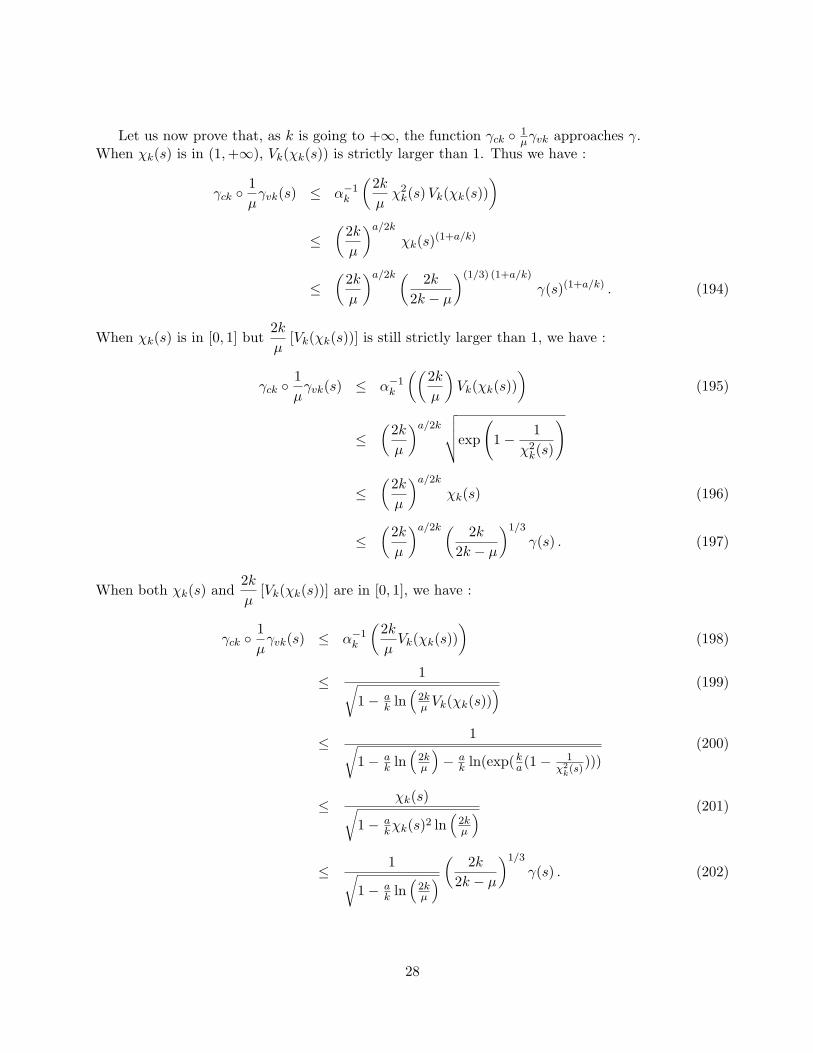
Let us now prove that, as k is going to +∞, the function γck ◦ 1µγvk approaches γ.

When χk(s) is in (1,+∞), Vk(χk(s)) is strictly larger than 1. Thus we have :

γck ◦1µ

γvk(s) ≤ α−1k

(2k

µχ2

k(s) Vk(χk(s)))

≤(

2k

µ

)a/2k

χk(s)(1+a/k)

≤(

2k

µ

)a/2k ( 2k

2k − µ

)(1/3) (1+a/k)

γ(s)(1+a/k) . (194)

When χk(s) is in [0, 1] but2k

µ[Vk(χk(s))] is still strictly larger than 1, we have :

γck ◦1µ

γvk(s) ≤ α−1k

((2k

µ

)Vk(χk(s))

)(195)

≤(

2k

µ

)a/2k√√√√exp

(1− 1

χ2k(s)

)

≤(

2k

µ

)a/2k

χk(s) (196)

≤(

2k

µ

)a/2k ( 2k

2k − µ

)1/3

γ(s) . (197)

When both χk(s) and2k

µ[Vk(χk(s))] are in [0, 1], we have :

γck ◦1µ

γvk(s) ≤ α−1k

(2k

µVk(χk(s))

)(198)

≤ 1√1− a

k ln(

2kµ Vk(χk(s))

) (199)

≤ 1√1− a

k ln(

2kµ

)− a

k ln(exp(ka(1− 1

χ2k(s)

)))(200)

≤ χk(s)√1− a

kχk(s)2 ln(

2kµ

) (201)

≤ 1√1− a

k ln(

2kµ

) ( 2k

2k − µ

)1/3

γ(s) . (202)

28

Combining (194), (197) and (202), we see that, for any strictly positive real number ε, there existssome integer K such that, for any k ≥ K,

γck ◦1µ

γvk(s) ≤

(1 + ε)γ(s) , if γ(s) ≤ 1 ,

(1 + ε) (γ(s))1+ε , if γ(s) > 1 .(203)

With (203), we conclude that, for the system (182), see that, by working with the exp-ISS gainfunction instead of the ISS gain function, we can get results which are as equally conservative as wewant on any compact set.

8 Conclusion

Consider the system : x = f(x) +

p∑i=1

gi(x) [ui + ci(x, z, u)] ,

z = a(x, z, u) .

(204)

Under the following conditions– the system :

x = f(x) +p∑

i=1

gi(x) ui (205)

is globally asymptotically stabilizable by a feedback law (uni(x)) (see A1),– the system : {

z = a(x, z, u)yi = ci(x, z, u)

(206)

has appropriate input-to-state and input-to-output properties (see A2 or A2’),we have shown how to modify the feedback un into a static or a dynamic feedback in order toguarantee that all the solutions of (204) are bounded and their x-components are captured by anarbitrarily small neighborhood of the origin. This result belongs to the broad class of results known onuncertain systems (see [C] for a survey and [Q1, Q2, KSK, KK, JMP] for some recent developments).

The modifications we have proposed for the control law un are based on Lyapunov design andgain assignment techniques as introduced in [JTP]. The analysis of the properties of the closed loopsystem is based on the application of the Small-Gain Theorem [JTP, Theorem 2.1]. The assumptionson the z-subsystem are written in terms of the notion of input-to-output stability (IOS) introducedin [JTP] which is an extension of the notion of input-to-state stability (ISS) as introduced by Sontagin [S2].

To carry out our design of a dynamic feedback, we have been led to introduce a new notionof ISS systems called exp-ISS. We have shown that for finite dimensional systems the two notionsare equivalent. For this we have used the link between the ISS property and the existence of anappropriate Lyapunov function which has been established in [LSW, SW].

An important feature of the system (204) is that the unmodelled effects are in the “range” of theinput. This is the well known matching assumption. By using arguments similar to those used for

29

propagating the ISS property through integrators in [JTP, Corollary 2.3], this matching assumptioncan be relaxed for systems and uncertainties having a recurrent so called feedback structure.

Acknowledgments

The authors would like to thank Miroslav Krstic, Jing Sun and Petar Kokotovic for making availableto them very early preprints of [KK, KSK] and Andrew Teel and Zhihua Qu for helpful discussionsand suggestions. The second author would also like to thank LAGEP, UCB Lyon I, France, for itshospitality where part of the work was carried out.

References

[BCL] B. R. Barmish, M. J. Corless, and G. Leitmann, A new class of stabilizing controllers foruncertain dynamical systems, SIAM Journal on Control and Optimization, 21 (1983), pp. 246–255.

[B] W. M. Boothby, An Introduction to Differentiable Manifold and Riemannian Geometry. SecondEdition. AP 1986.

[BIW] C. Byrnes, A. Isidori, J. Willems, Passivity, feedback equivalence and the global stabilizationof minimum phase nonlinear systems. IEEE Transactions on Automatic Control, 36, No. 11,(1991).

[C] M. J. Corless, Control of uncertain nonlinear systems, Journal of Dynamic Systems, Measure-ment, and Control, 115 (1993), pp. 362–372.

[CL] M. J. Corless and G. Leitmann, Continuous state feedback guaranteeing uniform ultimateboundedness for uncertain dynamic systems, IEEE Transactions on Automatic Control, 26(1981), pp. 1139–1144.

[G] S. Gutman, Uncertain dynamical systems — a Lyapunov min-max approach, IEEE Transactionson Automatic Control, 24 (1979), pp. 437–443.

[H] W. Hahn, Stability of Motion, Springer-Verlag, 1967

[I] A. Isidori, Nonlinear control systems, Second Edition. Springer Verlag 1989.

[J] Z.-P. Jiang, Quelques resultats de stabilisation robuste. Application a la commande, These deDocteur en Mathematiques et Automatique, Ecole des Mines de Paris, 1993.

[JMP] Z. P. Jiang, I.M.Y. Mareels, J.-B. Pomet, Output Feedback Global Stabilization for a Classof Nonlinear Systems with Unmodeled Dynamics. Accepted for publication in European Journalof Control, 1996.

[JP1] Z.-P. Jiang, L. Praly, Preliminary results about robust Lagrange stability in adaptive nonlinearregulation, Int. J. of Adaptive Control and Signal Processing, 6, No. 4, (1992).

30

[JP2] Z.-P. Jiang, L. Praly, Technical results for the study of robustness of Lagrange stability. Systems& Control Letters, 23 (1994), pp. 67–78

[JTP] Z.-P. Jiang, A. Teel, L. Praly, Small-gain theorem for ISS systems and applications, Mathe-matics of Control, Signals, and Systems, 7, (1994), pp. 95–120.

[K] H. K. Khalil, Nonlinear Systems, Macmillan, New York, 1992.

[KK] M. Krstic, P. Kokotovic, On extending the Praly-Jiang-Teel Design to systems with nonlinearinput unmodelled dynamics, Technical report CCEC 94-0211, February 1994

[KSK] M. Krstic, J. Sun, P. Kokotovic, Robust control of nonlinear systems with input unmodelleddynamics, Technical report CCEC 94-0125, January 1994

[LL] V. Lakshmikantham, S. Leela, Differential and integral ineaqualities : Theory and applications.Volume 1 : Ordinary differential equations, Academic Press, 1969.

[LSW] Y. Lin, E. Sontag, Y. Wang, A smooth converse Lyapunov theorem for robust stability, SIAMJournal on Control and Optimization, 34 (1996), No. 1, to appear.

[P] L. Praly, Almost exact modelling assumption in adaptive linear control, International Journalof Control, 51, No. 3, (1990), pp. 643-668.

[Q1] Z. Qu, Model reference robust control of SISO systems with significant unmodelled dynamics,Proc. of the American Control Conference , June 1993, pp. 255-259.

[Q2] Z. Qu, Model reference robust control of weakly non-minimum phase systems, Proc. of the 32ndIEEE Conference on Decision and Control, IEEE Publications, 1993, pp. 996–1000.

[SK] A. Saberi and H. K. Khalil, Quadratic-type Lyapunov functions for singularly perturbed sys-tems, IEEE Transactions on Automatic Control, 29, (1984), pp. 542–550.

[S1] E. D. Sontag, A “universal” construction of Artstein’s theorem on nonlinear stabilization, Sys-tems & Control Letters 13, (1989), 117-123.

[S2] E. D. Sontag, Smooth stabilization implies coprime factorization, IEEE Transactions on Auto-matic Control, 34, (1989), pp. 435–443.

[SW] E. D. Sontag, Y. Wang, On characterizations of the input-to-state stability property, Systems& Control Letters, 24, (1995), pp. 351–359.

31

Appendices

A On the non existence of a stabilizing feedback for (13).

We prove that there is no control law u(t) that can drive to zero the x-component of any solutionof (13), starting from (x0, 1) with x0 > M exp(1). To do this, let us assume that such a controlexists. By the uniqueness property, the corresponding solution (x(t), z(t)) of (13) remains in IR2

>0 forall positive time. Moreover, since

x(t) = exp(∫ t

0(x(s)− u(s) + γ(z(s))) ds

)x0 , ∀ t ≥ 0, (207)

we have, necessarily :

limt→∞

∫ t

0(u(s)− γ(z(s))− x(s))ds = +∞ . (208)

On the other hand, we have :dz

z2= (u(t)− z(t)) dt . (209)

With (14) and the fact that z(t) is strictly positive, (209) yields :

− 1z(t)

+ 1 =∫ t

0(u(s)− z(s))ds ≥

∫ t

0(u(s)−M − γ(z(s)))ds , (210)

and :1

z(t)≤ 1 −

∫ t

0(u(s)− γ(z(s))− x(s))ds −

∫ t

0x(s)ds + M t . (211)

Now let us define :t1 = inf

{t ≥ 0 :

∫ t

0(u(s)− γ(z(s))− x(s))ds ≥ 1

}. (212)

This real number is well defined (see (208)) and is positive. By continuity, we get :

x(t1) = x0 exp(−1) , (213)

1z(t1)

≤ 1 −∫ t1

0(u(s)− γ(z(s))− x(s))ds −

∫ t1

0x(s)ds + M t1

≤ − x0 t1exp(1)

+ M t1 . (214)

By the choice of x0, this yields that 1z(t1) < 0 which contradicts the fact that z(t) > 0 for all positive

t.

B An explicit expression for θi.

Working within the context of the proof of Lemma 3, we propose here an explicit expression for thefunction θi.

32

First of all, we define a function θi as :

θi(x) =

√(W (x)

2p

)2+ 3 (|LgiV (x)|ϕi(x))2 − W (x)

2p

|LgiV (x)|ϕi(x), if |LgiV (x)| 6= 0 ,

0 , if |LgiV (x)| = 0 ,

(215)

where :ϕi(x) = S(V (x)) + |uni(x)| . (216)

According to the arguments in the proof of [S1, Theorem 1], this function is continuous on IRn \ {0}.Moreover, we have :

x ∈ B1i =⇒(

W (x)2p

)2

+ 3 (|LgiV (x)|ϕi(x))2 ≥(

W (x)2p

+ |LgiV (x)|ϕ(x))2

. (217)

It follows that θi(x) is larger than 1 on B1i. This allows us to define θi on IRn\{0} as :

θi(x) = sat(θi(x)

), (218)

where sat : IR≥0 → [0, 1] is the saturation function :

sat(r) =

r , if r ∈ [0, 1] ,

1 , if r > 1 .(219)

33