
Stability of Queueing Networks - math.umn.edu - University of
189
Maury Bramson University of Minnesota Stability of Queueing Networks May 13, 2008 Springer Berlin Heidelberg NewYork Hong Kong London Milan Paris Tokyo
Transcript of Stability of Queueing Networks - math.umn.edu - University of

Maury BramsonUniversity of Minnesota
Stability of Queueing Networks
May 13, 2008
SpringerBerlin Heidelberg NewYorkHongKong LondonMilan Paris Tokyo

2
This manuscript will appear as Springer Lecture Notes in Mathematics 1950,Ecole d’Ete de Probabilites de Saint-Flour XXXVI-2006.
Copyright c© 2008 Springer-Verlag Berlin Heidelberg

Contents
1 Introduction . . . . . . . . . . . . . . . . . . . . . . . . . . . . . . . . . . . . . . . . . . . . . . . 51.1 The M/M/1 Queue . . . . . . . . . . . . . . . . . . . . . . . . . . . . . . . . . . . . . . 61.2 Basic Concepts of Queueing Networks . . . . . . . . . . . . . . . . . . . . . . 71.3 Queueing Network Equations and Fluid Models . . . . . . . . . . . . . 151.4 Outline of Lectures . . . . . . . . . . . . . . . . . . . . . . . . . . . . . . . . . . . . . . 18
2 The Classical Networks . . . . . . . . . . . . . . . . . . . . . . . . . . . . . . . . . . . . 212.1 Main Results . . . . . . . . . . . . . . . . . . . . . . . . . . . . . . . . . . . . . . . . . . . 222.2 Stationarity and Reversibility . . . . . . . . . . . . . . . . . . . . . . . . . . . . . 272.3 Homogeneous Nodes of Kelly Type . . . . . . . . . . . . . . . . . . . . . . . . 312.4 Symmetric Nodes . . . . . . . . . . . . . . . . . . . . . . . . . . . . . . . . . . . . . . . . 362.5 Quasi-Reversibility . . . . . . . . . . . . . . . . . . . . . . . . . . . . . . . . . . . . . . 43
3 Instability of Subcritical Queueing Networks . . . . . . . . . . . . . . 573.1 Basic Examples of Unstable Networks . . . . . . . . . . . . . . . . . . . . . . 583.2 Examples of Unstable FIFO Networks . . . . . . . . . . . . . . . . . . . . . . 643.3 Other Examples of Unstable Networks . . . . . . . . . . . . . . . . . . . . . 75
4 Stability of Queueing Networks . . . . . . . . . . . . . . . . . . . . . . . . . . . . 814.1 Some Markov Process Background . . . . . . . . . . . . . . . . . . . . . . . . . 844.2 Results for Bounded Sets . . . . . . . . . . . . . . . . . . . . . . . . . . . . . . . . . 964.3 Fluid Models and Fluid Limits . . . . . . . . . . . . . . . . . . . . . . . . . . . . 1044.4 Demonstration of Stability . . . . . . . . . . . . . . . . . . . . . . . . . . . . . . . . 1204.5 Appendix . . . . . . . . . . . . . . . . . . . . . . . . . . . . . . . . . . . . . . . . . . . . . . 131
5 Applications and Some Further Theory . . . . . . . . . . . . . . . . . . . . 1435.1 Single Class Networks . . . . . . . . . . . . . . . . . . . . . . . . . . . . . . . . . . . . 1445.2 FBFS and LBFS Reentrant Lines . . . . . . . . . . . . . . . . . . . . . . . . . . 1485.3 FIFO Networks of Kelly Type . . . . . . . . . . . . . . . . . . . . . . . . . . . . . 1515.4 Global Stability . . . . . . . . . . . . . . . . . . . . . . . . . . . . . . . . . . . . . . . . . 1595.5 Relationship Between QN and FM Stability . . . . . . . . . . . . . . . . . 167

4 Contents
Acknowledgments . . . . . . . . . . . . . . . . . . . . . . . . . . . . . . . . . . . . . . . . . . . . . 179
References . . . . . . . . . . . . . . . . . . . . . . . . . . . . . . . . . . . . . . . . . . . . . . . . . . . . . 181
Index . . . . . . . . . . . . . . . . . . . . . . . . . . . . . . . . . . . . . . . . . . . . . . . . . . . . . . . . . . 187

1
Introduction
Queueing networks constitute a large family of models in a variety of settings,involving “jobs” or “customers” that wait in queues until being served. Onceits service is completed, a job moves to the next prescribed queue, where itremains until being served. This procedure continues until the job leaves thenetwork; jobs also enter the network according to some assigned rule.
In these lectures, we will study the evolution of such networks and ad-dress the question: When is a network stable? That is, when is the underlyingMarkov process of the queueing network positive Harris recurrent? When thestate space is countable and all states communicate, this is equivalent to theMarkov process being positive recurrent. An important theme, in these lec-tures, is the application of fluid models, which may be thought of as being, ina general sense, dynamical systems that are associated with the networks.
The goal of this chapter is to provide a quick introduction to queueingnetworks. We will provide basic vocabulary and attempt to explain some ofthe concepts that will motivate later chapters. The chapter is organized asfollows. In Section 1.1, we discuss the M/M/1 queue, which is the “simplest”queueing network. It consists of a single queue, where jobs enter accordingto a Poisson process and have exponentially distributed service times. Theproblem of stability is not difficult to resolve in this setting.
Using M/M/1 queues as motivation, we proceed to more general queueingnetworks in Section 1.2. We introduce many of the basic concepts of queueingnetworks, such as the discipline (or policy) of a network determining whichjobs are served first, and the traffic intensity ρ of a network, which providesa natural condition for deciding its stability. In Section 1.3, we provide a pre-liminary description of fluid models, and how they can be applied to provideconditions for the stability of queueing networks.
In Section 1.4, we summarize the topics we will cover in the remainingchapters. These include the product representation of the stationary distri-butions of certain classical queueing networks in Chapter 2, and examples ofunstable queueing networks in Chapter 3. Chapters 4 and 5 introduce fluid

6 1 Introduction
models and apply them to obtain criteria for the stability of queueing net-works.
1.1 The M/M/1 Queue
The M/M/1 queue, or simple queue, is the most basic example of a queue-ing network. It is familiar to most probabilists and is simple to analyze. Wetherefore begin with a summary of some of its basic properties to motivatemore general networks.
The setup consists of a server at a workstation, and “jobs” (or “cus-tomers”) who line up at the server until they are served, one by one. Afterservice of a job is completed, it leaves the system. The jobs are assumed toarrive at the station according to a Poisson process with intensity 1; equiva-lently, the interarrival times of succeeding jobs are given by independent rate-1 exponentially distributed random variables. The service times of jobs aregiven by independent rate-µ exponentially distributed random variables, withµ > 0; the mean service time of jobs is therefore m = 1/µ. We are inter-ested here in the behavior of Z(t), the number of jobs in the queue at time t,including the job currently being served (see Figure 1.1).
Fig. 1.1. Jobs enter the system at rate 1 and depart at rate µ. There are currently2 jobs in the queue.
The process Z(·) can be interpreted in several ways. Because of the inde-pendent exponentially distributed interarrival and service times, Z(·) definesa Markov process, with states 0, 1, 2, . . .. (M/M/1 stands for Markov inputand Markov output, with one server.) It is also a birth and death process on{0, 1, 2, . . .}, with birth rate 1 and death rate µ. Because of the latter interpre-tation, it is easy to compute the stationary (or invariant) probability measureπm of Z(·) when it exists, since the process will be reversible. Such a measuresatisfies
πm(n + 1) = mπm(n) for n = 0, 1, 2, . . . ,
since it is constant, over time, on the intervals [0, n] and [n + 1,∞). It followsthat when m < 1, πm is geometrically distributed, with
πm(n) = (1 − m)mn, n = 0, 1, 2, . . . . (1.1)

1.2 Basic Concepts of Queueing Networks 7
All states clearly communicate with one another, and the process Z(·) ispositive recurrent. The mean of πm is m(1 − m)−1, which blows up asm ↑ 1. When m ≥ 1, no stationary probability measure exists for Z(·). Usingstandard reasoning, one can show that Z(·) is null recurrent when m = 1 andis transient when m > 1.
The behavior of Z(·) that was observed in the last paragraph provides thebasic motivation for these lectures, in the context of the more general queueingnetworks which will be introduced in the next section. We will investigatewhen the Markov process corresponding to a queueing network is stable, i.e.,is positive Harris recurrent. As mentioned earlier, this is equivalent to positiverecurrence when the state space is countable and all states communicate.
For M/M/1 queues, we explicitly constructed a stationary probabilitymeasure to demonstrate positive recurrence of the Markov process. Typically,however, such a measure will not be explicitly computable, since it will not bereversible. This, in particular, necessitates a new, more qualitative, approachfor showing positive recurrence. We will present such an approach in Chapter4.
1.2 Basic Concepts of Queueing Networks
The M/M/1 queue admits natural generalizations in a number of directions.It is unnecessary to assume that the interarrival and service distributions areexponential. For general distributions, one employs the notation G/G/1; orM/G/1 or G/M/1, if one of the distributions is exponential. (To emphasizethe independence of the corresponding random variables, one often uses thenotation GI instead of G.)
The single queue can be extended to a finite system of queues, or a queueingnetwork (for short, network), where jobs, upon leaving a queue, line up atanother queue, or station, or leave the system. The queueing network in Figure1.2 is also a reentrant line, since all jobs follow a fixed route.
j=1 j=2 j=3
Fig. 1.2. A reentrant line with 3 stations.
Depending on a job’s previous history, one may wish to prescribe differentservice distributions at its current station or different routing to the next

8 1 Introduction
station. This is done by assigning one or more classes, or buffers, to eachstation. Except when stated otherwise, we label stations by j = 1, . . . , J andclasses by k = 1, . . . , K; we use C(j) to denote the set of classes belonging tostation j and s(k) to denote the station to which class k belongs. In Figure1.3, there are 3 stations and 5 classes. Classes are labelled here in the orderthey occur along the route, with C(1) = {1, 5}, C(2) = {2, 4}, and C(3) = {3}.
j=3j=2j=1
Fig. 1.3. A reentrant line with 3 stations and 5 classes. The stations are labelledby j = 1, 2, 3; the classes are labelled by k = 1, . . . 5, in the order they occur alongthe route.
Other examples of queueing networks are given in Figures 1.4 and 1.5.Figure 1.4 depicts a network with 2 stations, each possessing 2 classes. Thenetwork is not a reentrant line but still exhibits deterministic routing, sinceeach job entering the network at a given class follows a fixed route. When theindividual routes are longer, it is sometimes more convenient to replace theabove labelling of classes by (i, k), where i gives the route that is followed andk the order of the class along the route.
j = 1 j = 2
Fig. 1.4. A queueing network having 3 routes, with 2 stations and 4 classes.

1.2 Basic Concepts of Queueing Networks 9
Figure 1.5 depicts a network with 2 stations and 3 classes. The routingat class 2 is random, with each job served there having probability 0.4 ofbeing sent to class 1 and probability 0.6 of being set to class 3. For queueingnetworks in general, we will assume that the interarrival times, service times,and routing of jobs at each class are given by sequences of i.i.d. randomvariables that are mutually independent (but whose distributions may dependon the class).
j = 2j = 1
k = 1
k = 2
k=3
0.4
0.6
Fig. 1.5. A queueing network with 2 stations and 3 classes. The random routing atclass 2 is labelled with the probability each route is taken.
Queueing networks occur naturally in a wide variety of settings. “Jobs”can be interpreted as products of some sort of complex manufacturing processwith multiple steps, as tasks that need to be performed by a computer orcommunication system, or as people moving about through a bureaucraticmaze. Such networks can be quite complicated. A portion of the procedure inthe manufacture of a semiconductor wafer is depicted by the reentrant line inFigure 1.6. Another simplified example, with classes emphasized, is given inFigure 1.7. Typically, such procedures can require hundreds of steps.
We will say that a queueing network is multiclass when at least one stationhas more than one class; otherwise, the network is single class. The term Jack-son network is frequently used for a single class network with exponentiallydistributed interarrival and service times, and generalized Jackson network isused for a single class network with arbitrary distributions. (The networks inFigures 1.3-1.7 are all multiclass; the networks in Figures 1.1–1.2 are singleclass.) Unless otherwise specified, it will be assumed that there is a singleserver at each station j. This server will be assumed to be non-idling (or workconserving), that is, it remains busy as long as there are jobs present at any

10 1 Introduction
Fig. 1.6. Part of the procedure in the manufacture of a semiconductor wafer. Theprocedure starts at the top and ends at the bottom. (Example courtesy of P. R.Kumar.)
k ∈ C(j). Stations are assumed to have infinite capacity, with jobs never beingturned away. (That is, there is no limit to the allowed length of queues.)
As already indicated, the interarrival times, service times, and routing ofjobs are given by sequences of independent random variables. Although theirspecific distributions will be relevant for some matters, their means will be ofmuch greater importance. We therefore introduce here the following notationand terminology for the means; systematic notation for the random variableswill be introduced in Chapter 4.
We denote by αk the rate at which jobs arrive at a class k from outsidethe network. When k ∈ A, the subset of classes where external arrivals areallowed, αk is the reciprocal of the corresponding mean interarrival time; whenk '∈ A, we set αk = 0. The vector α = {αk, k = 1, . . . , K} is referred to asthe external arrival rate. (Throughout the lectures, we interpret vectors ascolumn vectors unless stated otherwise.) We denote by mk, mk > 0, the meanservice time at class k, and by M the diagonal matrix with mk, k = 1, . . . , K,as its entries; we set µk = 1/mk, which is the service rate. We also denote

1.2 Basic Concepts of Queueing Networks 11
1
4
8/9
11
2
5/6
12
13
18/19
22/23
14
16
20/21
24
3
7
10
15
17FURNACE
ALIGN
IMPLANT
Enter
Fig. 1.7. Part of the procedure in the manufacture of another semiconductor wafer.(Example courtesy of J. G. Dai.)
by P = {Pk,!, k, $ = 1, . . . , K} the mean transition matrix (or mean routingmatrix), where Pk,! is the probability a job departing from class k goes toclass $. (In Figure 1.5, P2,1 = 0.4 and P2,3 = 0.6.)
In these lectures, we will be interested in open queueing networks , that is,those networks for which the matrix
Qdef= (I − PT )−1 = I + PT + (PT )2 + . . . (1.2)
is finite. (“ T ” denotes the transpose.) This means that jobs at any class arecapable of ultimately leaving the network. Closed queueing networks, whereneither arrivals to, nor departures from, the network are permitted, are notdiscussed here, although there are certain similarities between the two cases.
Disciplines for multiclass queueing networks
We have so far neglected an important aspect of multiclass queueing net-works. Namely, when more than one job is present at a station, what deter-mines the order in which jobs are served? There are numerous possibilities. Aswe will see in these lectures, the choice of the service rule, or discipline (alsoknown as policy), can have a major impact on the evolution of the queueingnetwork.
Perhaps the most natural discipline is first-in, first-out (FIFO), where thefirst job to arrive at a station (or “oldest” job) receives all of the service,irrespective of its class. (If the job later returns to the station, it starts overagain as the “youngest” job. The jobs originally at a class are assigned somearbitrary order.) Another widely used discipline is processor sharing (PS),where the service at a station is simultaneously equally divided between alljobs presently there. PS can be thought of as a limiting round robin discipline,

12 1 Introduction
where a server alternates among the jobs currently present at the station,dispensing a fixed small amount of service until it moves on to the next job.
The FIFO and PS disciplines are egalitarian in the sense that no job,because of its class, is favored over another. The opposite is the case for staticbuffer priority (SBP) disciplines, where classes are assigned a strict ranking,and jobs of higher ranked (or priority) classes are always served before jobs oflower ranked classes, irrespective of when they arrived at the station. Withina class, the jobs are served in the order of their arrival there. The disciplinesare called preemptive resume, or more simply, preemptive, if arriving higherranked jobs interrupt lower ranked jobs currently in service; when the serviceof such higher ranked jobs has been completed, service of lower ranked jobscontinues where it left off. If the service of lower ranked jobs is not interrupted,then the discipline is nonpreemptive.
For reentrant lines, two natural SBP disciplines are first-buffer-first-served(FBFS) and last-buffer-first-served (LBFS). For FBFS, jobs at earlier classesalong the route have priority over later classes. For example, jobs in class 1,in the network given in Figure 1.3, have priority over those in class 5, andjobs in class 2 have priority over those in class 4. For LBFS, the priority isreversed, with jobs at later classes along the route having priority over earlierclasses.
In these lectures, we will concentrate on head-of-the-line (HL) disciplines,where only the first job in each class of a station may receive service. (Thisproperty is frequently referred to as FIFO within a class.) FIFO and SBPdisciplines are HL, but PS is not. The single class networks we consider willalways be assumed to be HL unless explicitly stated otherwise. A major simpli-fying feature of HL disciplines is that the total amount of “work” (or “effort”)already devoted to partially served jobs does not build up. Since large num-bers of jobs will therefore tend not to complete service at a station at closetimes, this avoids “bursts” of jobs from being suddenly routed elsewhere inthe network.
Another non-HL discipline is last-in, first-out (LIFO), where the last jobto arrive at a station is served first. Other plausible non-HL disciplines from asomewhat different setting are first-in-system, first-out (FISFO) and last-in-system, first-out (LISFO). FISFO is the same as FIFO, except that the firstjob to enter the queueing network (rather than the station) has priority overother jobs; the discipline may be preemptive or nonpreemptive. LISFO givespriority to the last job to enter the network.
Throughout these lectures, the term queueing network will indicate thata discipline, such as FIFO or FBFS, has already been assigned to the system.In much of the literature, the discipline is specified afterwards. This linguisticdifference does not affect the theory, of course.
For the M/M/1 queue in the previous section, the interarrival and servicetimes were assumed to be exponentially distributed. As a consequence, theprocess Z(·) counting the number of jobs is Markov. For queueing networkswith exponentially distributed interarrival and service times, the situation

1.2 Basic Concepts of Queueing Networks 13
is often analogous. For instance, for preemptive SBP disciplines, the vectorvalued process Z(t) = {Zk(t), k = 1, . . . , K} counting the number of jobsat each class is Markov; the same is true for PS. For the FIFO and LIFOdisciplines, the process will be Markov if one appends additional informationgiving the order in which each job entered the class. In all of these cases, thestate space is countable, so one can apply standard Markov chain theory. Wewill denote by X(·) the corresponding Markov processes.
The situation becomes more complicated when the interarrival and ser-vice times are not exponentially distributed, since the residual interarrivaland service times need to be appended to the state in order for the process tobe Markov. The resulting state space is uncountable, and so a more generaltheory, involving Harris recurrence, is required for the corresponding Markovprocess. We will give a careful construction of such processes and will sum-marize the needed results on positive Harris recurrence at the beginning ofChapter 4. We avoid this issue until then, since the material in Chapters 2and 3 typically does not involve Markov processes on an uncountable statespace. (The sole exception is the uncountable state space extension for sym-metric processes at the end of Section 2.4.) In a first reading of the lectures,not too much will be lost by assuming the interarrival and service times areexponentially distributed.
Traffic intensity, criticality, and stability
The mean quantities α, M , and P introduced earlier perform an importantrole in determining the long-time behavior of a queueing network. To providemotivation, we first consider reentrant lines.
The (long term) rate at which jobs enter a reentrant line is α1, and themean time required to serve a job over all of its visits to a station j is∑
k∈C(j) mk. So, the rate at which future “work” for the station j enters thenetwork is
ρj = α1
∑
k∈C(j)
mk. (1.3)
We recall that a queueing network is defined to be stable when its un-derlying Markov process is positive Harris recurrent. When the state space iscountable and all states communicate, this is equivalent to the Markov processbeing positive recurrent. It is intuitively clear that, in order for a reentrantline to be stable, ρj ≤ 1, for all j, is necessary. Otherwise, by the law of largenumbers, the work in the system, corresponding to j, will increase linearly toinfinity as t → ∞, and so the same should be true for the total number of jobsin the system. (When the state space is countable, it follows from standardMarkov chain theory that a stable network must be empty a fixed fraction ofthe time, as t → ∞, from which it follows that, in fact, ρj < 1 must hold forall j.)
A natural condition for stability (assuming all states communicate), isthat ρj < 1 for all j. This turns out, in fact, not to be sufficient for multiclass

14 1 Introduction
queueing networks, as we will see in Chapter 3. Not surprisingly, the muchstronger condition ∑
j
ρj < 1 (1.4)
suffices for stability, since whenever the network is not empty, the total workin the network tends to decrease faster than it increases. (This will follow fromProposition 4.5.)
The situation is analogous for queueing networks with general routing,after the correct quantities have been introduced. We set
λ = Qα, (1.5)
and refer to the vector λ as the total arrival rate. (Recall that vectors are tobe interpreted as column vectors.) Its components λk, k = 1, . . . , K, are therates at which jobs enter the K classes; they each equal α1 for reentrant lines.The traffic equations
λ! = α! +∑
k
λkPk,!, (1.6)
or, in vector form, λ = α + PTλ, are equivalent to (1.5), and are useful incertain situations. Employing m and λ, we define the traffic intensity ρj atstation j to be
ρj =∑
k∈C(j)
mkλk. (1.7)
(ρj is also known as the nominal load.) The traffic intensity is the rate at whichwork for the station j enters the network, and reduces to (1.3) for reentrantlines. We write ρ for the corresponding traffic intensity vector.
We continue the analogy with reentrant lines, and say that a station jis subcritical if ρj < 1, critical if ρj = 1, and supercritical if ρj > 1. Whenall stations of a network are either subcritical or are critical, we refer to thenetwork as being subcritical or critical. We will sometimes abbreviate theseconditions by writing ρ < e and ρ = e, where e = (1, . . . , 1)T ; we similarlywrite ρ ≤ e,when ρj ≤ 1 for each j. When at least one station is supercritical,we refer to the network as being supercritical. As in the reentrant line setting,a supercritical queueing network will not be stable, and the number of jobsin the network will increase linearly as t → ∞. This is a bit tedious to showdirectly; it will follow quickly using fluid limits in Proposition 5.21. Of course,since a reentrant line with ρ < e need not be stable, the same is the casefor queueing networks with general routing. We will show in Chapters 4 and5, though, that the condition ρ < e is sufficient for the stability of queueingnetworks under various disciplines. Also, (1.4) suffices for stability irrespectiveof the discipline; a variant of this is shown in Example 1 at the end of Section4.4.
In Chapters 4 and 5, we will also establish criteria for when a queueingnetwork is e-stable. By this, we will mean that the underlying Markov process

1.3 Queueing Network Equations and Fluid Models 15
is ergodic, i.e., it possesses a stationary distribution π to which the distributionat time t converges in total variation norm as t → ∞, irrespective of the initialstate. When the state space is countable, this is equivalent to the probabilitiesconverging to π(x) at each point x. As we will see, results on stability can bemodified to results on e-stability with little additional work.
We have so far not used the term “unstable”. Somewhat different defi-nitions exist in the literature; in each case, they mean more than just “notstable”. For us, a queueing network will be unstable if, for some initial state,the number of jobs in the network will, with positive probability, go to infinityas t → ∞. (When the network has only a finite number of states with fewerthan a given number of jobs, and all states communicate with one another,this is equivalent to saying that for each initial state, the number of jobs in thenetwork goes to infinity almost surely as t → ∞.) According to the paragraphbefore the last, a supercritical queueing network will be unstable; in fact, thenumber of jobs in the network grows linearly in time. This will typically bethe case for unstable networks, such as those given in Chapter 3.
1.3 Queueing Network Equations and Fluid Models
One of the main themes in these lectures will be the application of fluid modelsto study the stability of queueing networks. Fluid models will be introducedand studied in detail in Chapter 4; they will then by applied to specific dis-ciplines in Chapter 5. We provide here some of the basic motivation for fluidmodels.
In the last section, we gave various examples of queueing networks. Suchsystems are frequently complicated. They can be interpreted as Markov pro-cesses, but to derive specific results, one needs a means of expressing theproperties of the specific queueing network. Queueing network equations pro-vide an analytic formulation for this. After deriving these equations and takingappropriate limits, one obtains the corresponding fluid models.
Queueing network equations tie together random vectors, such as A(t),D(t), T (t), and Z(t), that describe the evolution of a queueing network. Theindividual coordinates of these K dimensional vectors correspond, respec-tively, to the cumulative number of arrivals Ak(t) and departures Dk(t) at aclass k up to time t, the cumulative time Tk(t) spent serving this class up totime t, and the number of jobs Zk(t) at this class at time t; we introducedZ(t) in the last section. Examples of queueing network equations are
A(t) = E(t) +∑
k
Φk(Dk(t)), (1.8)
Z(t) = Z(0) + A(t) − D(t), (1.9)Dk(t) = Sk(Tk(t)), k = 1, . . . , K. (1.10)

16 1 Introduction
We are employing here the following terminology. The vector E(t) is thecumulative number of jobs arriving by time t at each class from outside thenetwork (i.e., external arrivals). When the interarrival times are exponentiallydistributed, E(·) will be a Poisson process. The vector Φk(dk) is the numberof the first dk departures from class k that are routed to each of the K classes;Sk(tk) is the cumulative number of departures from class k after tk units ofservice there. We will denote by Φ and S the matrix and vector correspondingto these quantities.
The quantities E(·), S(·), and Φ(·) should be thought of as random, butknown input into the system, from which the evolution of A(·), D(·), T (·),and Z(·) will be determined via (1.8)–(1.10) and other equations. The middleequation is easiest to read, and just says that the number of jobs at time t isequal to the original number, plus arrivals, and minus departures. The firstequation says the total number of arrivals is equal to the number of externalarrivals plus the number of arrivals from other classes; the last equation givesthe number of departures at a class as a function of the time spent serving jobsthere. We note that the first two equations hold irrespective of the discipline,whereas the last equation requires the discipline to be HL.
Other choices of variables, in addition to A(·), D(·), T (·) and Z(·), are fre-quently made. We will include other variables, such as the immediate workloadW (·), in our detailed treatment in Section 4.3. Often, different formulationsof the queueing network equations are equivalent, with the exact format be-ing chosen for convenience. One can, for example, eliminate A(t) and D(t) in(1.8)–(1.10), and instead employ the single equation
Z(t) = Z(0) + E(t) +∑
k
Φk(Sk(Tk(t)) − S(T (t)), (1.11)
if one is just interested in the evolution of Z(t) (which is most often the case).Note that, for multiclass networks, neither (1.8)–(1.10) nor (1.11) suppliesenough information to solve for the unknown variables, since the discipline hasnot been specified, and so T (·) has not been uniquely determined. To specifythe discipline, an additional equation (or equations) is required. For singleclass networks, this complication is not present. As an elementary example,note that for the M/M/1 queue, (1.11) reduces to the simple scalar equation
Z(t) = Z(0) + E(t) − S
(∫ t
01 {Z(s) > 0} ds
), (1.12)
since departing jobs are not rerouted into the queue and the network is non-idling.
Fluid model equations are the deterministic analog of queueing networkequations, with one replacing the random quantities E(·), S(·), and Φ(·) bytheir corresponding means. The fluid model equations corresponding to (1.8)-(1.10) are then

1.3 Queueing Network Equations and Fluid Models 17
A(t) = αt + PT D(t), (1.13)Z(t) = Z(0) + A(t) − D(t), (1.14)Dk(t) = µkTk(t), k = 1, . . . , K, (1.15)
where α, P , and µk were defined in the previous section. By employing thematrix M , one can also write (1.15) as
D(t) = M−1T (t). (1.15′)
Similarly, the fluid model equation corresponding to (1.11) is
Z(t) = Z(0) + αt + (PT − I)M−1T (t). (1.16)
For the M/M/1 queue, this reduces to the scalar equation
Z(t) = Z(0) + αt − µ
∫ t
01 {Z(s) > 0} ds. (1.17)
Fluid model equations can be thought of as belonging to a fluid networkwhich is the deterministic equivalent of the given queueing network. Jobs arereplaced by continuous fluid mass (or “job mass”), which follows the samerouting as before. The constant rate at which such mass enters the network isgiven by the vector α. The rate at which mass is served for a class is µk andthe service time per unit mass is mk = 1/µk. A set of fluid model equations,as in (1.13)–(1.15), is referred to collectively as a fluid model.
The solutions of fluid models are frequently much easier to analyze than arethe corresponding queueing network equations. As we will see in Chapter 4,fluid model equations can be derived from the corresponding queueing networkequations by taking limits of Z(·) and the other quantities after hydrodynamicscaling. (That is, “law of large numbers” scaling of the form Z(st)/s as s →∞.) Fluid models will provide a valuable tool for demonstrating the stabilityof queueing networks, as we will see in Chapters 4 and 5. Fluid models arealso an important tool for studying heavy traffic limits, which lie outside thescope of these lectures.
To analyze the stability of a queueing network, one introduces the followingnotion of stability for a fluid model. A fluid model is said to be stable if thereexists an N > 0, so that for any solution of the fluid model equations, its Z(·)component satisfies
Z(t) = 0 for t ≥ N |Z(0)|. (1.18)
(Here, | · | denotes the $1 norm.) We will show in Chapter 4 that, under certainconditions on the interarrival and service times, a queueing network will bestable if its fluid model is stable.
In the special case of the fluid model equation (1.17) corresponding to theM/M/1 queue, it is easy to explicitly solve for Z(·). For µ > α, the solutiondrifts linearly to 0 at rate µ − α, after which it remains there, and so

18 1 Introduction
Z(t) = 0 for t ≥ Z(0)/(µ− α), (1.19)
which is a special case of (1.18). This behavior of the solution of equation(1.17) corresponding to a subcritical M/M/1 queue is not surprising, since thesolution Z(·) of (1.12) possesses the same negative drift α−µ when Z(t) > 0.For more general networks, one typically constructs a Lyapunov function withrespect to which the fluid model solution Z(·) of (1.16) exhibits a uniformlynegative drift until hitting 0.
Despite the utility of fluid models, one needs to exercise some caution intheir application. In particular, a fluid model need not have a unique solutionfor a given initial condition, since solutions might bifurcate. As we will see inSection 4.3, this can be the case even for certain standard disciplines. (Suchbehavior might occur at times when there are two or more empty multiclassstations.) On account of this, thinking of fluid model equations as belongingto a fluid network loses some of its appeal. In practice, it is often better tothink directly in terms of the fluid model which is defined by the appropriatesystem of equations.
1.4 Outline of Lectures
We conclude the introduction with an outline of the subject matter we willbe covering. The material can be broken into three parts, Chapter 2, Chapter3, and Chapters 4 and 5, each with its own distinct character.
Chapter 2 discusses the “classical” queueing networks introduced in[BaCMP75] and the accompanying theory of quasi-reversible queueing net-works in [Ke79]. The examples considered in [BaCMP75] include networkswith the FIFO, PS, and LIFO disciplines that were introduced in Section 1.2,and an infinite server network, which we will introduce in Chapter 2. Expo-nentially distributed interarrival times, and in some cases, exponentially dis-tributed service times, are assumed. For ρ < e, these networks are stable andexplicit product-like formulas are given for their stationary distributions. Thisspecial structure is a generalization of that for the M/M/1 queue. Independentwork of F. P. Kelly, leading to the book [Ke79], employed quasi-reversibilityto show that these explicit formulas hold in a more general setting. Theseresults have strongly influenced the development of queueing theory over thepast several decades.
In the previous sections, we mentioned that even when ρ < e, a queueingnetwork may be unstable. This behavior came as a surprise in the early 1990’s.Various examples of instability have since been given in different settings,primarily in the context of SBP and FIFO disciplines. At this point, there isno comprehensive theory, and in fact, not much is known, in general, abouthow the Markov processes for such networks go to infinity as t → ∞. Chapter3 presents the best known examples of unstable subcritical queueing networksin more-or-less chronological order, with an attempt being made to provide

1.4 Outline of Lectures 19
some feeling for the development of the subject. Examples include those from[LuK91],[RyS92], [Br94a], [Se94], and [Du97].
In Chapter 4, we give general sufficient conditions for the stability of aqueueing network. The main condition is that the fluid model of the queueingnetwork be stable; general conditions on the interarrival and service times ofthe queueing network are also needed. In the previous section, we gave a briefdiscussion of how the fluid model equations are obtained from the queueingnetwork equations that describe the evolution of the queueing network. Thematerial in Chapter 4 is largely based on [Da95] and the sources employedthere. We go into considerable detail on the arguments leading to the mainresult, Theorem 4.16, because we feel that it is important to have this materialaccessible in one place.
The first part of Chapter 5 consists of applications of Theorem 4.16, wherestability is demonstrated, under ρ < e, for a number of disciplines. In Sections5.1, 5.2, and 5.3, the stability of single class networks, SBP reentrant lines withFBFS and LBFS priority schemes, and FIFO networks, with constant meanservice times at a station, are demonstrated. In each case, the procedure isto demonstrate the stability of a fluid model; the stability of the queueingnetwork then follows by applying the above theorem.
Sections 5.4 and 5.5 are different in nature from the previous three sections.Section 5.4 is concerned with the question of global stability. That is, whenis a queueing network stable, irrespective of the particular discipline that isapplied? Again applying Theorem 4.16, a queueing network will be globallystable if its fluid model is. For two-station fluid models with deterministicrouting, a complete theory is given. Section 5.5 investigates the converse ofTheorem 4.16, namely the necessity of fluid model stability for the stability ofa given queueing network. It turns out that there is not an exact correspon-dence between the two types of stability, as examples show. Robust conditionsfor the necessity of fluid model stability are presently lacking. The materialin Chapter 5 is taken from a member of sources, including [Br96a], [DaWe96],[Br99], [DaV00], and [DaHV04].
We conclude this section with some basic notation and conventions. We letZ+ and R+ denote the positive integers and real numbers; Z+,0 and R+,0 willdenote the sets appended with {0}; and Zd
+, Rd+, Zd
+,0, and Rd+,0 will denote
their d dimensional equivalents. For x, y ∈ Rd, x ≤ y means xk ≤ yk foreach coordinate k; x < y means xk < yk for each coordinate. Unless indicatedotherwise, | · | denotes the $1 (or sum) norm, e.g., |x| =
∑di=1 |xi| for x ∈ Rd.
By a∨ b and a ∧ b, we mean max{a, b} and min{a, b}. For x ∈ R, by ,x- and.x/, we mean the integer part of x and the smallest integer that is at least x.By a(t) ∼ b(t), we mean a(t)/b(t) → 1 as t → ∞, and by a ≈ b, that a and bare approximately the same in some weaker sense.
When convenient, we will refer to a countable state Markov process as aMarkov chain. (In the literature, Markov chain often instead refers to a dis-crete time Markov process.) We say that a Markov chain is positive recurrentif each state is positive recurrent and all states communicate. (The second

20 1 Introduction
condition is sometimes not assumed in the literature.) As already mentioned,instead of the term “queueing network”, we will often employ the shorter “net-work”, when the context is clear. Throughout these lectures, continuous timestochastic processes will be assumed to be right continuous unless indicatedotherwise.

2
The Classical Networks
In this chapter, we discuss two families of queueing networks whose Markovprocesses are positive recurrent when ρ < e, and whose stationary distribu-tions have explicit product-like formulas. The first family includes networkswith the FIFO discipline, and the second family includes networks with thePS and LIFO disciplines, as well as infinite server (IS) networks. We intro-duced the first three networks in Section 1.2; we will define infinite servernetworks shortly. These four networks are sometimes known as the “classicalnetworks”. Together with their generalizations, they have had a major influ-ence on the development of queueing theory because of the explicit natureof their stationary distributions. For this reason, we present the basic resultsfor the accompanying theory here, although only the FIFO discipline is HL.These results are primarily from [BaCMP75], and papers by F. P. Kelly (suchas [Ke75] and [Ke76]) that led to the book [Ke79].
In Section 2.1, we state the main results in the context of the above fournetworks. We first characterize the stationary distributions for networks con-sisting of a single station, whose jobs exit from the network when service iscompleted, without being routed to another class. We will refer to such a sta-tion as a node. We then characterize the stationary distribution for networkswith multiple stations and general routing. Since all states will communicate,the Markov processes for the networks will be positive recurrent, and hencethe networks will be stable.
In the remainder of the chapter, we present the background for these resultsand the accompanying theory. In Section 2.2, we give certain basic propertiesof stationary and reversible Markov processes on countable state spaces thatwe will use later. Sections 2.3 and 2.4 apply this material to obtain generaliza-tions of the node-level results in Section 2.1 to the two families of interest tous. The first family, homogeneous nodes, includes FIFO nodes under certainrestrictions, and the second family, symmetric nodes, includes PS, LIFO, andIS nodes.
The concept of quasi-reversibility is introduced in Section 2.5. Using quasi-reversibility, the stationary distributions of certain queueing networks can be

22 2 The Classical Networks
written as the product of the stationary distributions of nodes that correspondto the stations “in isolation”. These queueing networks include the FIFO, PS,LIFO, and IS networks, and so generalize the network-level results in Section2.1. Except for Theorem 2.9, all of the material in this chapter is for queueingnetworks with a countable state space.
The main source of the material in this chapter is [Ke79]. Section 2.2 isessentially an abridged version of the material in Chapter 1 of [Ke79]. Mostof the material in Sections 2.3-2.5 is from Sections 3.1-3.3 of [Ke79], with[Wa88], [ChY01], [As03], and lecture notes by J.M. Harrison having also beenconsulted. The order of presentation here, starting with nodes in Sections 2.3and 2.4 and ending with quasi-stationarity in Section 2.5, is different.
2.1 Main Results
In this section, we will give explicit formulas for the stationary distributionsof FIFO, PS, LIFO, and infinite server networks. Theorems 2.1 and 2.2 statethese results for individual nodes, and Theorem 2.3 does so for networks. InSections 2.3-2.5, we will prove generalizations of these results.
The range of disciplines that we consider here is of limited scope. Onthe other hand, the routing that is allowed for the network-level results willbe completely general. As in Chapter 1, routing will be given by a meantransition matrix P = {Pk,!, k, $ = 1, . . . , K} for which the network is open.1For all queueing networks considered in this section, the interarrival timesare assumed to be exponentially distributed. When the service times are alsoexponentially distributed, the evolution of these queueing networks can beexpressed in terms of a countable state Markov process. By enriching the statespace, more general service times can also be considered in the countable statespace setting. This will be useful for the PS, LIFO, and IS networks.
In Section 1.1, we introduced the M/M/1 queue with external arrival rateα = 1. By employing the reversibility of its Markov process when m < 1, wesaw that its stationary distribution is given by the geometric distribution in(1.1). Allowing α to be arbitrary with αm < 1, this generalizes to
π(n) = (1 − αm)(αm)n for n = 0, 1, 2, . . . . (2.1)
For a surprisingly large group of queueing networks, generalizations of (2.1)hold, with the stationary distribution being given by products of terms similarto those on the right side of (2.1).1 In the literature (such as in [Ke79]), deterministic routing is frequently employed.
For these lectures, we prefer to use random routing, which was used in [BaCMP75]and has been promulgated in its current form by J. M. Harrison. By employingsufficiently many routes, one can show the two approaches are equivalent. Wefind the approach with random routing to be notationally more flexible. Theformulation is also more amenable to problems involving dynamic scheduling,which we do not cover here.

2.1 Main Results 23
We first consider queueing networks consisting of just a single node. Thatis, jobs at the unique station leave the network immediately upon completionof service, without being routed to other classes. Classes are labelled k =1, . . . , K. The nodes of interest to us in this chapter fall into two basic families,depending on the discipline.
The first family, homogeneous nodes, will be defined in Section 2.3. FIFOnodes, which are the canonical example for this family, will be considered here.For homogeneous nodes, including FIFO nodes, we need to assume that themean service times mk at all classes k are equal. In order to avoid confusionwith the vector m, we label such a service time by ms (with “s” standingfor “station”). We will refer to such a node as a FIFO node of Kelly type. Inaddition to assuming the interarrival times are exponentially distributed, weassume the same is true for the service times.
The state x of the node at any time will be specified by an n-tuple of theform
(x(1), . . . , x(n)), (2.2a)
where n is the number of jobs in the node and
x(i) ∈ {1, . . . , K} for i = 1, . . . , n (2.2b)
gives the class of the job in the ith position in the node. We interpret i =1, . . . , n as giving the order of arrival of the jobs currently in the node; becauseof the FIFO discipline, all service is directed to the job at i = 1. The statespace S0 will be the union of these states. The stochastic process X(t), t ≥ 0,thus defined will be Markov with a countable state space. For consistency withother chapters, we interpret vectors as column vectors, although this is notneeded in the present chapter (since matrix multiplication is not employed).
All states communicate with the empty state. So, if X(·) has a stationarydistribution, it will be unique. Since there is only a single station, a stationarydistribution will exist when the node is subcritical. Theorem 2.1 below gives anexplicit formula for the distribution. As in Chapter 1, αk denotes the externalarrival rates at the different classes k; ρ denotes the traffic intensity and is inthe present setting given by the scalar
ρ = ms∑
k
αk. (2.3)
As elsewhere in this chapter, when we say that a node (or queueing network)has a stationary distribution, we mean that its Markov process, on the chosenstate space, has this distribution. (For us, “distribution” is synonymous withthe somewhat longer “probability measure”.)
Theorem 2.1. Each subcritical FIFO node of Kelly type has a stationarydistribution π, which is given by
π(x) = (1 − ρ)n∏
i=1
msαx(i), (2.4)

24 2 The Classical Networks
for x = (x(1), . . . , x(n)) ∈ S0.
The stationary distribution π in Theorem 2.1 can be described as follows.The probability of there being a total of n jobs in the node is (1−ρ)ρn. Givena total of n jobs, the probability of there being n1, . . . , nK jobs at the classes1, . . . , K, with n = n1 + . . . + nK and no attention being paid to their order,is
ρ−n
(n
n1, . . . , nK
) K∏
k=1
(msαk)nk . (2.5)
Moreover, given that there are n1, . . . , nK jobs at the classes 1, . . . , K, any or-dering of the different classes of jobs is equally likely. Note that since all stateshave positive probability of occurring, the process X(·) is positive recurrent.Consequently, the node is stable.
The other family of nodes that will be discussed in this chapter, symmetricnodes, will be defined in Section 2.4. Standard members of this family are PS,LIFO, and IS nodes. The PS and LIFO disciplines were specified in Chapter 1.In an infinite server (IS) node, each job is assumed to start receiving service assoon as it enters the node, which it receives at rate 1. One can therefore thinkof there being an infinite number of unoccupied servers available to provideservice, one of which is selected whenever a job enters the node. All otherdisciplines studied in these lectures will have only a single server at a givenstation. We note that although the PS discipline is not HL, it is related to theHLPPS discipline given at the end of Section 5.3.
We consider the stationary distributions of PS, LIFO and IS nodes. Aswith FIFO nodes, we need to assume that the interarrival times of jobs areexponentially distributed. If we assume that the service times are also expo-nentially distributed, then the process X(·) defined on S0 will be Markov. Asbefore, we interpret the coordinates i = 1, . . . , n in (2.2) as giving the order ofjobs currently in the node. For LIFO nodes, this is also the order of arrival ofjobs there. For reasons relating to the definition of symmetric nodes in Section2.4, we will instead assume, for PS and IS nodes, that arriving jobs are, withequal probability 1/n, placed at one of the n positions of the node, where nis the number of jobs present after the arrival of the job. Since in both cases,jobs are served at the same rate irrespective of their position in the node, theprocesses X(·) defined in this manner are equivalent to the processes definedby jobs always arriving at the rear of the node.
The analog of Theorem 2.1 holds for PS, LIFO, and IS nodes when theservice times are exponentially distributed. We no longer need to assume thatthe service times have the same means, so in the present setting, the trafficintensity ρ is given by
ρ =∑
k
mkαk. (2.6)
For subcritical PS and LIFO nodes, the stationary distribution π is given by

2.1 Main Results 25
π(x) = (1 − ρ)n∏
i=1
mx(i)αx(i), (2.7)
for x = (x(1), . . . , x(n)) ∈ S0. For any IS node, the stationary distribution πis given by
π(x) =e−ρ
n!
n∏
i=1
mx(i)αx(i). (2.8)
The stability of the infinite server node for all values of ρ is not surprising,since the total rate of service at the node is proportional to the number ofjobs presently there.
For PS, LIFO, and IS nodes, an analogous result still holds when exponen-tial service times are replaced by service times with more general distributions.One employs the “method of stages”, which is defined in Section 2.4. One en-riches the state space S0 to allow for different stages of service for each job,with a job advancing to its next stage of service after service at the previousstage has been completed. After service at the last stage has been completed,the job leaves the node. Since the service times at each stage are assumed tobe exponentially distributed, the corresponding process X(·) for the node, onthis enriched state space Se, will still be Markov. On the other hand, the totalservice time required by a given job will be the sum of the exponential servicetimes at its different stages, which we take to be i.i.d. Such service times aresaid to have Erlang distributions.
Using the method of stages, one can extend the formulas (2.7) and (2.8),for the stationary distributions of PS, LIFO, and IS nodes, to nodes that haveservice distributions which are countable mixtures of Erlang distributions.This result is stated in Theorem 2.2. The state space here for the Markovprocess X(·) of the node is Se, which is defined in Section 2.4. The analog ofthis extension for FIFO nodes is not valid.
Theorem 2.2. Each subcritical PS node and LIFO node, whose service timedistributions are mixtures of Erlang distributions, has a stationary distributionπ. The probability of there being n jobs in the node with classes x(1), . . . , x(n)is given by (2.7). The same is true for any IS node with these service timedistributions, but with (2.8) replacing (2.7).
Mixtures of Erlang distributions are dense in the set of distribution func-tions, so it is suggestive that a result analogous to Theorem 2.2 should holdfor service times with arbitrary distributions. This is in fact the case, althoughone needs to be more careful here, since one needs to replace Se with an un-countable state space which specifies the residual service times of jobs at thenode. More detail on this setting is given at the end of Section 2.4. Becauseof the technical difficulties for uncountable state spaces, (2.7) and (2.8) aretypically stated for mixtures of Erlang distributions or other related distribu-tions on countable state spaces. Moreover, quasi-reversibility, which we discussshortly, employs a countable state space setting.

26 2 The Classical Networks
So far in this section, we have restricted our attention to nodes. As men-tioned at the beginning of the section, the results in Theorems 2.1 and 2.2extend to analogous results for queueing networks, which are given in Theo-rem 2.3, below. FIFO, PS, LIFO, and IS queueing networks are the analogsof the respective nodes, with jobs at individual stations being subjected tothe same service rules as before, and, upon completion of service at a class k,a job returning to class $ with probability Pk,!, which is given by the meantransition matrix P . In addition to applying to these queueing networks, The-orem 2.3 also applies to networks that are mixtures of such stations, with oneof the above four rules holding for any particular station. We also note thatthe formula in Theorem 2.3 holds for Jackson networks, as a special case ofFIFO networks. The product formula for Jackson networks in [Ja63] predatesthose for the other networks.
In Theorem 2.3, we assume that the service times are exponentially dis-tributed when the station is FIFO, and are mixtures of Erlang distributionsin the other three cases. The distribution function π is defined on the statespace
S = S1 × . . . × SJ ,
where Sj = S0 if j is FIFO and Sj = Se for the other cases, and πj is definedon Sj . (The choice of K in each factor depends on Sj .)
Theorem 2.3. Suppose that each station j of a queueing network is eitherFIFO of Kelly type, PS, LIFO, or IS. Suppose that in the first three cases, thestation is subcritical. Then, the queueing network has a stationary distributionπ that is given by
π(x) =J∏
j=1
πj(xj), (2.9)
for x = (x1, . . . , xJ). Here, each πj is either of the form (2.4), (2.7), or (2.8),depending on whether the station j is FIFO of Kelly type, PS or LIFO, or IS,and αk in the formulas is replaced by λk.
Theorem 2.3 will be a consequence of Theorems 2.1 and 2.2, and of thequasi-reversibility of the nodes there. Quasi-reversibility will be introduced inSection 2.5. Using quasi-reversibility, it will be shown, in Theorem 2.11, thatthe stationary distributions of certain queueing networks can be written asthe product of the stationary distributions of nodes that correspond to theindividual stations “in isolation”. This will mean that when service of a job ata class is completed, the job will leave the network rather than returning toanother class (either at the same or a different station). The external arrivalrates αk at classes are replaced by the total arrival rates λk of the networkin order to compensate for the loss of jobs that would return to them. Quasi-reversibility can be applied to queueing networks whose stations are FIFO,PS, LIFO, or IS. By employing Theorem 2.11, one obtains Theorem 2.3 as aspecial case of Theorem 2.12.

2.2 Stationarity and Reversibility 27
2.2 Stationarity and Reversibility
In this section, we will summarize certain basic results for countable state,continuous time Markov processes. We define stationarity and reversibility,and provide alternative characterizations. Proposition 2.6, in particular, willbe used in the remainder of the chapter.
The Markov processes X(t), t ≥ 0, we consider here will be assumed tobe defined on a countable state space S. The space S will be assumed tobe irreducible, that is, all states communicate. None of the states will beinstantaneous; we will assume there are only a finite number of transitionsafter a finite time, and hence no explosions. Sample paths will therefore beright continuous with left limits. The transition rate between states x and ywill be denoted by q(x, y); the rate at which a transition occurs at x is thereforeq(x) def=
∑y∈S q(x, y). The embedded jump chain has mean transition matrix
{p(x, y), x, y ∈ S}, where p(x, y) def= q(x, y)/q(x) is the probability X(·) nextvisits y from the state x. The time X(·) remains at a state x before a transitionoccurs is exponentially distributed with mean 1/q(x).
A stochastic process X(t), t ≥ 0, is said to be stationary if (X(t1), . . . ,X(tn)) has the same distribution as (X(t1 + u), . . . , X(tn + u)), for eachnonnegative t1, . . . , tn and u. Such a process can always be extended to−∞ < t < ∞ so that it is stationary as before, but with t1, . . . , tn and unow being allowed to assume any real values. When X(·) is a Markov process,it suffices to consider just n = 1 in order to verify stationarity.
A stationary distribution π = {π(x), x ∈ S} for a Markov process X(·)satisfies the balance equations
π(x)∑
y∈S
q(x, y) =∑
y∈S
π(y)q(y, x) for x ∈ S, (2.10)
which say that the rates at which mass leaves and enters a state x are thesame. We are assuming here that
∑x∈S π(x) = 1. Since all states are assumed
to communicate, π will be unique. If π exists, then it is the limit of the dis-tributions of the Markov process starting from any initial state. If a measureπ satisfying (2.10) with
∑x∈S π(x) < ∞ exists, then it can be normalized so
that∑
x∈S π(x) = 1. If∑
x∈S π(x) = ∞, then there is no stationary distribu-tion, and for all x, y ∈ S,
P (X(t) = $ | X(0) = x) → 0 as t → ∞.
(See, e.g., [Re92] for such basic theory.)A stochastic process X(t), −∞ < t < ∞, is said to be reversible if
(X(t1), . . . , X(tn)) has the same distribution as (X(u − t1), . . . , X(u − tn)),for each t1, . . . , tn and u. This condition says that the process is stochasti-cally indistinguishable, whether it is run forward or backwards in time. It iseasy to see that if X(·) is reversible, then it must be stationary. When X(·)

28 2 The Classical Networks
is Markov, it suffices to consider n = 2 in order to verify reversibility. TheMarkov property can be formulated as saying that the past and future statesof the process X(·) are independent given the present. It follows that the re-versed process X(t) def= X(−t) is Markov exactly when X(·) is. If X(·) hasstationary measure π, then π is also stationary for X(·) and the transitionrates of X(·) are given by
q(x, y) =π(y)π(x)
q(y, z) for x, y ∈ S. (2.11)
A stationary Markov process X(·) with distribution π is reversible exactlywhen it satisfies the detailed balance equations
π(x)q(x, y) = π(y)q(y, x) for x, y ∈ S. (2.12)
This condition says that the rate at which mass moves from x to y is the samerate at which it moves in the reverse direction. This condition need not, ofcourse, be satisfied for arbitrary stationary distributions. When (2.12) holds,it often enables one to express the stationary distribution in closed form, as,for example, for the M/M/1 queue in Section 1.1. It will always hold for thestationary distribution of any birth and death process, and, more generally,for the stationary distribution of any Markov process on a tree. By summingover $, one obtains the balance equations in (2.10) from (2.12).
An alternative characterization of reversibility is given by Proposition 2.4.We will not employ the proposition elsewhere, but state it because it providesuseful intuition for the concept.
Proposition 2.4. A stationary Markov process is reversible if and only if itstransition rates satisfy
q(x1, x2)q(x2, x3) · · · q(xn−1, xn)q(xn, x1) (2.13)= q(x1, xn)q(xn, xn−1) · · · q(x3, x2)q(x2, x1),
for any x1, x2, . . . , xn.
The equality (2.13) says that the joint transition rates of the Markovprocess are the same along a path if it starts and ends at the same point,irrespective of its direction along the path.
Proof of Proposition 2.4. The “only if” direction follows immediately by plug-ging (2.12) into (2.13).
For the “if” direction, fix x0, and define
π(x) =n∏
i=1
[q(xi−1, xi)/q(xi, xi−1)], (2.14)
where xn = x and x0, x1, . . . , xn is any path from x0 to x, with q(xi, xi−1) > 0.One can check using (2.13) that the right side of (2.14) does not depend on the

2.2 Stationarity and Reversibility 29
particular path that is chosen, and so π(x) is well defined. To see this, let P1
and P2 be any two paths from x0 to x, and P1 and P2 be the correspondingpaths in the reverse directions. Then, the two paths from x0 to itself formedby linking P1 to P2, respectively P2 to P1, satisfy (2.13), from whence theuniqueness in (2.14) will follow.
Assume that for given y, q(y, x) > 0. Multiplication of both sides of (2.14)by q(x, y) implies that
π(x)q(x, y) = q(y, x)
(n∏
i=1
q(xi−1, xi)/q(xi, xi−1
)(q(x, y)/q(y, x))
= q(y, x)π(y).
This gives (2.12), since the case q(x, y) = q(y, x) = 0 is trivial. Since theprocess is assumed to be stationary,
∑x π(x) < ∞, and so π can be scaled so
that∑
x π(x) = 1.
The following result says that under certain modifications of the transitionrates q(x, y), a reversible Markov process will still be reversible. It will not beneeded for later work, but has interesting applications.
Proposition 2.5. Suppose that the transition rates of a reversible Markovprocess X(·), with state space S and stationary distribution π, are altered bychanging q(x, y) to q′(x, y) = bq(x, y) when x ∈ A and y '∈ A, for some A ⊆S. Then, the resulting Markov process X ′(·) is reversible and has stationarydistribution
π′(x) =
{cπ(x) for x ∈ A,
cbπ(x) for x '∈ A,(2.15)
where c is chosen so that∑
x π′(x) = 1. In particular, when the state space
is restricted to A by setting b = 0, then the stationary distribution of X ′(·) isgiven by
π′(x) = π(x)/∑
y∈A
π(y) for x ∈ A. (2.16)
Proof. It is easy to check that q′ and π′ satisfy the detailed balance equationsin (2.12).
The following illustration of Proposition 2.5 is given in [Ke79].
Example 1. Two queues with a joint waiting room. Suppose that two inde-pendent M/M/1 queues are given, with external arrival rates αi and meanservice times mi, and αimi < 1. Let Xi(t) be the number of customers (orjobs) in each queue at time t. The Markov processes are each reversible withstationary distributions as in (2.1). It is easy to check that the joint Markovprocess X(t) = (X1(t), X2(t)), −∞ < t < ∞, is reversible, with stationarydistribution

30 2 The Classical Networks
π(n1, n2) = (1 − α1m2)(1 − α2m2)(α1m1)n1(α2m2)n2 for ni ∈ Z+,0.
Suppose now that the queues are required to share a common waiting roomof size N , so that a customer who arrives to find N customers already thereleaves without being served. This corresponds to restricting X(·) to the setA of states with n1 + n2 ≤ N . By Proposition 2.5, the corresponding processX ′(·) is reversible, and has stationary measure
π′(n1, n2) = π(0, 0)(α1m1)n1(α2m2)n2 for (n1, n2) ∈ A.
It is often tedious to check the balance equations (2.10) in order to de-termine that a Markov process X(·) is stationary. Proposition 2.6 gives thefollowing alternative formulation. We abbreviate by setting
q(x) =∑
y∈S
q(x, y), q(x) =∑
y∈S
q(x, y), (2.17)
where q(x, y) are the transition rates for X(·) and q(x, y) ≥ 0 are for themoment arbitrary. When X(·) has stationary distribution π and q(x, y) isgiven by (2.11), it is easy to check that
q(x) = q(x) for all x. (2.18)
The proposition gives a converse to this. As elsewhere in this section, we areassuming that S is irreducible.
Proposition 2.6. Let X(t), −∞ < t < ∞, be a Markov process with transi-tion rates {q(x, y), x, y∈S}. Suppose that for given quantities {q(x, y), x, y∈S} and {π(x), x∈S}, with q(x, y) ≥ 0, π(x) > 0, and
∑x π(x) = 1, that q,
q, and π satisfy (2.11) and (2.18). Then, π is the stationary distribution ofX(·) and q gives the transition rates of the reversed process.
Proof. It follows, by applying (2.11) and then (2.18), that∑
x∈S
π(x)q(x, y) = π(y)∑
x∈S
q(y, x) = π(y)q(y) = π(y)q(y).
So, π is stationary for X(·). The transition rates of the reversed process aretherefore given by (2.11).
Proposition 2.6 simplifies the computations needed for the demonstrationof stationarity by replacing the balance equations, that involve a large sumand the stationary distribution π, by two simpler equations, (2.18), whichinvolves just a large sum, and (2.11), which involves just π. On the otherhand, the application of Proposition 2.6 typically involves guessing q and π.In situations where certain choices suggest themselves, the proposition can bequite useful. It will be used repeatedly in the remainder of the chapter.

2.3 Homogeneous Nodes of Kelly Type 31
2.3 Homogeneous Nodes of Kelly Type
FIFO nodes of Kelly type belong to a larger family of nodes whose station-ary distributions have similar properties. We will refer to such a node as ahomogeneous node of Kelly type. Such nodes are defined as follows.
Consider a node with K classes. The state x ∈ S0 of the node at any timeis specified by an n-tuple as in (2.2), when there are n jobs present at thenode. The ordering of the jobs is assumed to remain fixed between arrivals andservice completions of jobs. When the job in position i completes its service,the position of the job is filled with the jobs in positions i+1, . . . , n moving upto positions i, . . . , n− 1, while retaining their previous order. Similarly, whena job arrives at the node, it is assigned some position i, with jobs previouslyat positions i, . . . , n being moved back to positions i + 1, . . . , n + 1. Each jobrequires a given random amount of service; when this is attained, the jobleaves the node. As throughout this chapter, interarrival times are requiredto be exponentially distributed. As elsewhere in these lectures, all interarrivaland service times are assumed to be independent.
We will say that such a node is a homogeneous node if it also satisfies thefollowing properties:
(a) The amount of service required by each job is exponentially distributedwith mean mk, where k is the class of the job.
(b) The total rate of service supplied at the node is φ(n), where n is thenumber of jobs currently there.
(c) The proportion of service that is directed at the job in position i is δ(i, n).Note that this proportion does not depend on the class of the job.
(d) When a job arrives at the node, it moves into position i, i = 1, . . . , n, withprobability β(i, n), where n is the number of jobs in the node includingthis job. Note that this probability does not depend on the class of thejob.
When the mean mk does not depend on the class k, we will say that sucha node is a homogeneous node of Kelly type. We will analyze these nodes inthis section. We use ms when the mean service times of a node are constant,as we did in Section 2.1.
The rate at which service is directed to a job in position i is δ(i, n)φ(n).So, the rate at which service at the job is completed is δ(i, n)φ(n)/ms. Wewill assume that φ(n) > 0, except when n = 0. The rate at which a job arrivesat a class k and position i from outside the node is αkβ(i, n). We use herethe mneumonics β and δ to suggest births and deaths at a node. Of course,∑n
i=1 β(i, n) =∑n
i=1 δ(i, n) = 1.We have emphasized in the above definition that the external arrival rates
and service rates β and δ do not depend on the class of the job. This is crucialfor Theorem 2.7, the main result in this section. This restriction will also be

32 2 The Classical Networks
needed in Section 2.4 for symmetric nodes, as will be our assumption thatthe interarrival times are exponentially distributed. On the other hand, theassumptions that the service times be exponential and that their means mk
be constant, which are needed in this section, are not needed for symmetricnodes. We note that by scaling time by 1/ms, one can set ms = 1, althoughwe prefer the more general setup for comparison with symmetric nodes andfor application in Section 2.5.
In Section 2.5, we will be interested in homogeneous queueing networks ofKelly type. Homogeneous queueing networks are defined analogously to homo-geneous nodes. Jobs enter the network independently at the different stationsaccording to exponentially distributed random variables, and are assignedpositions at these stations as in (d). Jobs at different stations are served inde-pendently, as in (a)-(c), with departing jobs from class k being routed to class$ with probability Pk,! and leaving the network with probability 1 −Σ!Pk,!.Jobs arriving at a class $ from within the network are assigned positions as in(d), according to the same rule as was applied for external arrivals. The ex-ternal arrival rates and the quantities in (a)-(d) are allowed to depend on thestation. When the mean service times mk are assumed to depend only on thestation j = s(k), we may write ms
j ; we refer to such networks as homogeneousqueueing networks of Kelly type.
The most important examples of homogeneous nodes are FIFO nodes.Here, one sets φ(n) ≡ 1,
β(i, n) =
{1 for i = n,
0 otherwise,
and
δ(i, n) =
{1 for i = 1,
0 otherwise,
for n ∈ Z+. That is, arriving jobs are always placed at the end of the queueand only the job at the front of the queue is served. Another example is givenin [Ke79], where arriving jobs are again placed at the end of the queue, butwhere L servers are available to serve the first L jobs, for given L. In thissetting, φ(n) = L ∧ n, β is defined as above, and
δ(i, n) =
1/n for i ≤ n ≤ L,
1/L for i ≤ L < n,
0 for i > L.
The main result in this section is Theorem 2.7, which is a generalizationof Theorem 2.1. Since the total service rate φ that is provided at the nodecan vary, the condition
Bdef=
∞∑
n=0
(ρn
/ n∏
i=1
φ(i)
)< ∞ (2.19)

2.3 Homogeneous Nodes of Kelly Type 33
replaces the assumption in Theorem 2.1 that the node is subcritical. Here,ρ = ms
∑Kk=1 αk is the traffic intensity.
Theorem 2.7. Suppose that a homogeneous node of Kelly type satisfies B <∞ in (2.19). Then, it has a stationary distribution π that is given by
π(x) = B−1n∏
i=1
(msαx(i)/φ(i)), (2.20)
for x = (x(1), . . . , x(n)) ∈ S0.
As was the case in Theorem 2.1, the structure of the stationary distributionπ in Theorem 2.7 exhibits independence at multiple levels. The probability ofthere being a total of n jobs at the node is ρn/B
∏ni=1 φ(i). Given a total of
n jobs at the node, the probability of there being n1, . . . , nk jobs of classes1, . . . , K, respectively, is given by the multinomial distribution in (2.5). More-over, the ordering of the different classes of jobs is equally likely. As was thecase in Theorem 2.1, all states communicate with the empty state, and theMarkov process X(·) for the node is positive recurrent.
Demonstration of Theorem 2.7
The proof of Theorem 2.7 that we will give is based on Proposition 2.6.In order to employ the proposition, we need to choose quantities q and π sothat (2.11) and (2.18) are satisfied for them and the transition rates q of theMarkov process X(·) for the node. It will then follow from Proposition 2.6that π is the stationary distribution for the node and q gives the transitionrates for the reversed process X(·). A similar argument will be used again forsymmetric nodes in Section 2.4 and for networks consisting of quasi-reversiblenodes in Section 2.5. We will summarize a more probabilistic argument forTheorem 2.7 at the end of the section.
In order to demonstrate Theorem 2.7, we write q and our choices for qand π explicitly in terms of α, β, δ, and φ. To be able to reuse this argumentin Section 2.4 for symmetric nodes, we write mk for the mean service times,which in the present case reduces to the constant ms.
The nonzero transition rates q(x, y) take on two forms, depending onwhether the state is obtained from x by the arrival or exit of a job. In theformer case, we write y = ak,i(x) if a class k job arrives at position i; in thelatter case, it follows that x = ak,i(y), if i is the position of the exiting classk job. One then has
q(x, y) =
{αkβ(i, ny) for y = ak,i(x),m−1
k δ(i, nx)φ(nx) for x = ak,i(y),(2.21)
where nx and ny are the number of jobs at the node for states x and y.Finding the transition rates q(x, y) of the reversed process involves some
guessing, motivated by our idea of what X(·) should look like. It is reasonable

34 2 The Classical Networks
to guess that X(·) is also the Markov process for a homogeneous node. Theexternal arrival rates αk and αk will then be the same for both processes,since arrivals for X(·) correspond to exits for X(·), and under the stationarydistribution π, the two rates must be the same. The mean service times mk
and mk will also be the same. It is reasonable to guess that φ(n) = φ(n);this would be the case if X(·) were reversible, as it is for the M/M/1 queue.Running X(·) backwards in time mentally, it is also tempting to set
β(i, n) = δ(i, n), δ(i, n) = β(i, n) for n ∈ Z+, i ≤ n.
For instance, if the original node is FIFO, then jobs arrive at i = n and exitat i = 1; if the node is run backwards in time, jobs arrive at i = 1 and exit ati = n. Substitution of these choices for α, β, δ, φ, and m in (2.21) yields
q(x, y) =
{αkδ(i, ny) for y = ak,i(x),m−1
k β(i, nx)φ(nx) for x = ak,i(y).(2.22)
We still need to choose our candidate for the stationary distribution π ofboth X(·) and X(·). The equality (2.11), that is needed for Proposition 2.6,is equivalent to
π(x)q(x, y) = π(y)q(y, x) (2.23)
holding whenever y = ak,i(x) or x = ak,i(y). When y = ak,i(x) and q(x, y) > 0,substitution of (2.21) and (2.22) into (2.23) implies that
π(y)/π(x) = mkαk/φ(ny). (2.24)
The case x = ak,i(y) yields the same equality, but with the roles of x and yreversed. Reasoning backwards, it is not difficult to see that (2.23) also followsfrom (2.24).
Set x = (x(1), . . . , x(n)), for n ∈ Z+,0. One can repeatedly apply (2.24) byremoving jobs from x one at a time, starting from the last, until the emptystate is reached. We therefore choose π so that
π(x) = B−1n∏
i=1
(mx(i)αx(i)/φ(i)), (2.25)
where the normalizing constant B = 1/π(∅). Under (2.25), (2.24) must hold.We have therefore verified (2.11) for this choice of π. In particular, this holdsfor mk ≡ ms, as in Theorem 2.7.
In order to employ Proposition 2.6, we also need to verify (2.18). One cancheck that ∑
y
q(x, y) =∑
k
αk + φ(nx)∑
i
m−1x(i)δ(i, nx). (2.26)
The first sum on the right side of (2.26) follows by summing the top line of(2.21) over all i and k. The relationship x = ak,i(y) implies that x(i) = k, and

2.3 Homogeneous Nodes of Kelly Type 35
so the last sum in (2.26) follows by summing the last line of (2.21) over all i.Using the same reasoning, one obtains the formula
∑
y
q(x, y) =∑
k
αk + φ(nx)∑
i
m−1x(i)β(i, nx) (2.27)
from (2.22). As before, the first sum on the right side is obtained from arrivingjobs and the last sum is obtained from exiting jobs.
We see from (2.26) and (2.27) that a sufficient condition for (2.18) is that∑
i
m−1x(i)δ(i, nx) =
∑
i
m−1x(i)β(i, nx). (2.28)
In Theorem 2.7, mk ≡ ms, which factors outside of the sum on both sides of(2.28). Since the resulting sums both equal 1, (2.28), and hence (2.18), holdsin this setting. Note that this is the only point in the argument at which weneed mk to be constant.
We have shown that both (2.11) and (2.18) are satisfied for q and q′ givenby (2.21) and (2.22), and π given by (2.25), under the assumptions in Theorem2.7. It therefore follows from Proposition 2.6 that π is the stationary distri-bution for the Markov process with transition rates q. This implies Theorem2.7.
Some observations
One can generalize the above proof of Theorem 2.7 so that it applies to ho-mogeneous queueing networks of Kelly type, rather than to just homogeneousnodes of Kelly type as in the theorem. Then, the stationary distribution π canbe written as the product of stationary distributions πj of nodes correspond-ing to the individual stations, when they operate “in isolation”. This is donein Section 3.1 of [Ke79]. We prefer to postpone the treatment of homogeneousnetworks until Section 2.5, where they are considered within the context ofquasi-reversibility.
One can give a more probabilistic proof of Theorem 2.7 that is based onthe following intuitive argument. The rates β(i, n), δ(i, n) and φ(n) governingthe arrival and service rates of jobs, as well as the mean service time ms, donot distinguish between classes of jobs. Jobs are therefore served as they wouldbe for an M/M/1 queue modified to have the total rate of service φ(n), whenthere are n jobs, and having the arrival rate
∑k αk. By randomly choosing the
class of each job, with probability αk/∑
k αk for each k, at either time 0 or atsome later time t, the distributions at time t of the two resulting processes willbe the same. If the stationary distribution for the modified M/M/1 queue ischosen as its initial distribution, the resulting distribution π′ for the K classeswill therefore also be stationary.
One can show, by using reversibility, that the probability of there be-ing n jobs for the stationary distribution of the modified M/M/1 queue isρn/B
∏ni=1 φ(i), where B is as in (2.19). Because of the random way in which

36 2 The Classical Networks
the classes of jobs are chosen above for π′, the remaining properties in thealternative characterization of π in (2.20), that are given after the statementof Theorem 2.7, also hold. Therefore, π′ = π, as desired.
We also note the following consequence of the proof of Theorem 2.7, thatis a special case of phenomena that will be discussed in Section 2.5. (It alsofollows from the alternative argument that was sketched above.) The transi-tion rates q of the reversed Markov process X(·) in (2.22) are the rates for ahomogeneous node of Kelly type. For this reversed node, arrivals are thereforegiven by K independent Poisson processes for the different classes, that areindependent of the initial state. These arrivals correspond to exiting jobs forthe original homogeneous node. It follows that the K different exit processesfor the classes are also independent Poisson processes that are independent ofany future state of the node.
2.4 Symmetric Nodes
PS, LIFO, and IS nodes all belong to the family of symmetric nodes. Theyare defined similarly to the homogeneous nodes of Kelly type in the previoussection, with a few major differences. The basic framework is the same, withstate space S0 given by (2.2) and existing jobs being reordered as before uponthe arrival and departure of jobs at the node. Moreover, the interarrival timesare exponentially distributed.
In order for such a node to be a symmetric node, we require that it alsosatisfy the following properties:
(a) The amount of service required by each job is exponentially distributedwith mean mk. We will soon allow more general distributions, but this willrequire us to extend the state space.
(b) The total rate of service supplied at the node is φ(n), where n is thenumber of jobs currently there.
(c) The proportion of service that is directed at the job in position i is β(i, n).Note that the proportion does not depend on the class of the job.
(d) When a job arrives at the node, it moves into position i, i = 1, . . . , n, withprobability β(i, n), where n is the number of jobs in the node includingthis job. This function is the same as that given in (c).
In Section 2.5, we will also be interested in symmetric queueing networks.These networks are defined analogously, with properties (a)-(d) being assumedto hold at each station, and departing jobs from a class k being routed to aclass $ with probability Pk,!. More detail is given in Section 2.3 for homoge-neous networks, where the procedure is the same.
The properties (a)-(d) given here are more restrictive than the properties(a)-(d) in the previous section in that we now assume, in the notation of

2.4 Symmetric Nodes 37
Section 2.3, that δ = β, in parts (c) and (d). These properties are moregeneral in that the service time means mk need no longer be equal at differentclasses. After comparing the stationary distributions of these nodes with thoseof Section 2.3, we proceed to generalize the exponential distributions of theservice times in (a) in two steps, first to mixtures of Erlang distributions, andthen to arbitrary distributions.
The PS, LIFO, and IS nodes are standard examples of symmetric nodes.For the PS discipline, one sets
β(i, n) = 1/n for i ≤ n,
for n ∈ Z+, and for LIFO, one sets
β(i, n) =
{1 for i = n,
0 otherwise.
In both cases, φ(n) ≡ 1. For IS nodes, φ(n) = n and
β(i, n) = 1/n for i ≤ n.
The analog of Theorem 2.7 holds for symmetric nodes when B < ∞, forB in (2.19), with the formula for the stationary distribution π,
π(x) = B−1n∏
i=1
(mx(i)αx(i)/φ(i)), (2.29)
for x = (x(1), . . . , x(n)), replacing (2.20). One can check that the same ar-gument as before is valid. One applies Proposition 2.6, for which one needsto verify (2.11) and (2.18). As before, the formulas for q and q are given by(2.21) and (2.22), but with δ = β. The formula for π is given by (2.25).
The argument we gave for (2.11) involved no restrictions on mk, and there-fore holds in the present context as well. The argument we gave for (2.18)consisted of equating (2.26) and (2.27), and therefore verifying (2.28). Pre-viously, (2.28) held since m−1
k was constant, and so could be factored out ofboth sums. It is now satisfied since δ = β, and so the summands are identical.One can therefore apply Proposition 2.6, from which the analog of Theorem2.7 for symmetric nodes follows, with (2.29) replacing (2.20).
The method of stages
As mentioned earlier, the assumption that the service times be expo-nentially distributed is not necessary for symmetric nodes. By applying themethod of stages, one can generalize the service time distributions to mixturesof Erlang distributions. (These are gamma distributions that are convolutionsof identically distributed exponential distributions.) We will show that theanalog of the formula (2.29) for the stationary distribution continues to holdin this more general setting.

38 2 The Classical Networks
In order for the stochastic process corresponding to the node to remainMarkov for more general service times, we need to enrich the state spaceS0. For this, we replace each coordinate x(i) in (2.2) by the triple x(i) =(x(i), s(i), v(i)), where
x(i) ∈ {1, . . . , K}, s(i) ∈ Z+, v(i) ∈ {1, . . . , s(i)}. (2.30)
Such a triple gives the refined class of a job, with x(i) denoting its class asbefore. The third coordinate v(i) gives the current stage of a job, with s(i)denoting the total number of stages the job visits before leaving the node. Thestate space Se will consist of such n-tuples x = (x(1), . . . ,x(n)), n ∈ Z+,0,under a mild restriction to ensure all states are accessible.
The basic dynamics of the node are the same as before, which satisfies theproperties for symmetric nodes given at the beginning of the section, includingproperties (b)-(d); we are generalizing here the assumption in (a). Instead ofentering the node at a class k with rate αk, jobs enter at a refined class (k, s, s)with rate αkpk(s), where
∑s pk(s) = 1. Once at a refined class (k, s, v), such
a job moves to (k, s, v − 1) after completing its service requirement, which isexponentially distributed with mean mk(s). After a job completes its serviceat the stage v = 1, it leaves the node. The current stage v of a job can thereforebe thought of as the residual number of stages remaining before the job leavesthe node. We note that the proportion of service that is directed at a job inposition i is β(i, n), which does not depend on its class or refined class.
The distribution of the service time that is required for the job betweenentering and leaving class k is a mixture of Erlang distributions, and has mean
mkdef=
∑
s
spk(s)mk(s). (2.31)
The state space Se mentioned earlier is defined to consist of n-tuples whosecomponents (k, s, v) satisfy pk(s) > 0, in order to exclude inaccessible states.Under this restriction, all states will communicate. The state space is of coursecountable. When pk(1) = 1 at all k, the service times are all exponentiallydistributed and the model reduces to the one considered at the beginning ofthe section. As with homogeneous and symmetric nodes with exponentiallydistributed service times, the networks corresponding to symmetric nodes withstages can be defined in the natural way.
We wish to show that the nodes just defined have stationary distributionsπ that generalize (2.29). This result is stated in Theorem 2.8.
Theorem 2.8. Suppose that the service times of a symmetric node are mix-tures of Erlang distributions, and that the node satisfies B < ∞ in (2.19).Then, the node has a stationary distribution π that is given by
π(x) = B−1n∏
i=1
(px(i)(s(i))mx(i)(s(i))αx(i)/φ(i)), (2.32)
where x = (x(1), . . . ,x(n)) ∈ Se and x(i) = (x(i), s(i), v(i)), for i = 1, . . . , n.

2.4 Symmetric Nodes 39
As was the case in Theorem 2.7 and in (2.29), the structure of the station-ary distribution π is Theorem 2.8 exhibits independence at multiple levels.The probability of there being a total of n jobs at the node is ρn/B
∏ni=1 φ(i).
Given a total of n jobs at the node, the probability of there being n1, . . . , nk
jobs at the classes 1, . . . , K is given by the multinomial
ρ−n
(n
n1, . . . , nK
) K∏
k=1
(mkαk)nk . (2.33)
The ordering of these classes is equally likely. Note that none of these quanti-ties depends on the particular service time distributions, except for the meansmk.
The stationary distribution also has the following refined structure. Giventhe class of the job at each position i, the probability of the job at a givenposition, whose class is k, having refined class (k, x, v) is
pk(s)mk(s)/mk,
and these events are independent at different i. Summing over all stagesstrictly greater than v and over all s, while keeping everything else fixed,this implies that the conditional probability of the job at position i being ina strictly earlier stage than v is
m−1k
∑
s
(s − v)pk(s)mk(s). (2.34)
Note that (2.34) depends on the actual service time distributions, and notjust on their means.
Demonstration of Theorem 2.8
In order to demonstrate Theorem 2.8, we employ Proposition 2.6. To doso, we need to verify (2.11) and (2.18) for the transition rates q of the Markovprocess on Se corresponding to the node, with an appropriate choice of thequantities q and π.
In order to specify q and q, we modify the function ak,i(·) we used forexponential service times on the state space S0. Here, ak,s,i(x) will denotethe state y obtained from state x by the arrival of a job at position i, withrefined class (k, s, s). Since jobs exit from the node at refined classes of theform (k, s, 1) (rather than at (k, s, s)), we need additional notation. With aneye on defining q, we denote by ak,s,i(x) the state y that is obtained from xby inserting a job with refined class (k, s, 1) at i; the positions of jobs alreadyat the node are shifted in the usual way. We also denote by si(x) the statey obtained from a state x satisfying 2 ≤ v(i) ≤ s(i), when the stage at iadvances to v(i) − 1. (si(x) is not defined for other x.)
Using this notation, one can check that q is given by

40 2 The Classical Networks
q(x, y) =
αkpk(s)β(i, ny) for y = ak,s,i(x),(mk(s))−1β(i, nx)φ(nx) for x = ak,s,i(y),(mk(s))−1β(i, nx)φ(nx) for y = si(x),
(2.35)
with q(x, y) = 0 otherwise. Employing the same motivation as in Section 2.3,we choose q so that
q(x, y) =
αkpk(s)β(i, ny) for y = ak,s,i(x),(mk(s))−1β(i, nx)φ(nx) for x = ak,s,i(y),(mk(s))−1β(i, ny)φ(ny) for x = si(y),
(2.36)
with q(x, y) = 0 otherwise. The transition function q is the same as q, exceptthat jobs arrive at the stage v = 1, exit at v = s(i), with changes in stageoccurring from v − 1 to v, for 2 ≤ v ≤ s(i). We choose π as in (2.32).
The assumptions for Proposition 2.6 can be verified as they were in Section2.3 for the space S0, with only a small change in argument. The argument for(2.11) is the same when either y = ak,s,i(x) or x = ak,s,i(y). For y = ak,s,i(x),the equality (2.24) is replaced by its analog
π(y)/π(x) = mk(s)pk(s)αk/φ(ny).
When y ∈ si(x), one has
π(y)/π(x) = q(x, y)/q(y, x) = 1, (2.37)
in which case (2.11) is obvious. So, (2.11) holds in all cases. (Note that for thehomogeneous nodes in Section 2.3 with distinct β and δ, the analog of (2.37)does not hold, and so the method of stages employed here for generalizing theexponential distributions will not work.)
The formula (2.18) holds for the same reasons as before, except that onenow has
∑
y
q(x, y) =∑
y
q(x, y) =∑
k
αk + φ(nx)∑
i
(mx(i)(s(i)))−1β(i, nx),
with mx(i)(s(i)) replacing mx(i). So, the assumptions for Proposition 2.6 hold.Application of the proposition therefore implies Theorem 2.8.
One can generalize the above argument so that it applies to symmetricqueueing networks. Then, the stationary distribution π can be written as theproduct of stationary distributions πj of nodes corresponding to the individualstations. As in the previous section, we choose to postpone the treatment ofsymmetric networks until Section 2.5, where they are considered within thecontext of quasi-reversibility.

2.4 Symmetric Nodes 41
Extensions to general distributions
We have employed the method of stages to generalize the formula (2.29),for the stationary distribution of symmetric nodes with exponentially dis-tributed service times, to the formula (2.32), which holds for service timesthat are mixtures of Erlang distributions. The method of stages can also beemployed to construct service times with other distributions. This approach isemployed, for example, in Section 3.6 of [Wa88] and in Section 3.4 of [As03],where the more general phase-type distributions are constructed. [As03] alsogives further background on the problem.
Let H =⋃∞
N=1 HN , where HN denotes the family of mixtures of Erlangdistributions, but with the restriction that mk(s) = 1/N for all k and s. It isnot difficult to show that H is dense in the set of distribution functions, withrespect to the weak topology; this result is given in Exercise 3.3.3 in [Ke79].The basic idea is that the sum of Ns i.i.d. copies of an exponential distribu-tion, with mean 1/N , has mean s and variance s/N , and so, for large N , isconcentrated around s. For large enough N , one can therefore approximate agiven service time distribution function Fk as closely as desired, by setting
pNk (s) = FN
k (s/N) − FNk ((s − 1)/N), for s ∈ Z+, (2.38)
equal to the probability that a job chooses a refined class with s stages,when it enters class k. Here, FN
k is the distribution function satisfyingFN
k (s′) = Fk(s′), for Ns′ ∈ Z+, and which is constant off this lattice. Forthe same reason, the phase-type distributions that were mentioned in theprevious paragraph are also dense.
Since the family H of mixtures of Erlang distributions is dense, it is tempt-ing to infer that a stationary distribution will always exist for a symmetricnode with any choice of service time distributions Fk satisfying (2.19), withmk replacing ms in the definition of ρ, and that this distribution has the sameproduct structure as given below the statement of Theorem 2.8. Such a resultholds, although the state space needs to be extended so that the last com-ponent v of the refined class (k, s, v) of a job can now take on any value in(0, s]; this corresponds to the residual service time of that job. The resultingstate space S∞ for the Markov process is uncountable; this causes technicalproblems which we discuss at the end of the section. Since the space is un-countable, it is most natural to formulate the result in a manner similar tothat given below Theorem 2.8.
Theorem 2.9. Suppose that a symmetric node satisfies B < ∞ in (2.19).Then, it has a stationary distribution π on S∞ with
π(x(i) = k(i), i = 1, . . . , n) = B−1n∏
i=1
(mk(i)αk(i)/φ(i)). (2.39)
Conditioned on any such set, the residual service times of the different jobsare independent, with the probability that a job of a class k has residual servicetime at most r being

42 2 The Classical Networks
F ∗k (r) =
1mk
∫ r
0(1 − Fk(s))ds. (2.40)
One can motivate (2.39) by applying Theorem 2.8 to a sequence of nodesindexed by N , with pN
k for each class k being given by (2.38). Since FNk ⇒ Fk
and mNk → mk as N → ∞, one should expect (2.39) to follow from (2.32). In
order to motivate (2.40), one can reason as follows. Applying Theorem 2.8,one can check that, under the stationary distribution πN and conditioned onthe job at a given position being k, the probability that the stage there isstrictly greater than v is
∑
s>v
(s − v)pNk (s)
/∑
s
spNk (s).
One can also check that∑
s>v(s−v)pNk (s) =
∑s>v FN
k (s/N), where FNk (s) =
1 − FNk (s). So, the above quantity equals
1N
∑
s>v
FNk (s/N)
/1N
∑
s
FNk (s/N).
By setting v = Nr, r ≥ 0, and applying the Monotone Convergence Theoremto the numerator and denominator separately, one obtains the limit
1mk
∫ ∞
rFk(s)ds. (2.41)
On the other hand, the same reasoning as above (2.38) implies that, forlarge N , the stage v scaled by N typically approximates the residual servicetime. So, (2.41) will also give the limiting distribution of the residual servicetimes as N → ∞. Taking the complementary event, one obtains (2.40) from(2.41).
The same reasoning as above implies (2.40) is also the probability that theamount of service that has been received by a job is at least r. We point outthat F ∗
k , as in (2.40), is the distribution of the residual time for the stationarydistribution of a renewal process, with lifetime distribution Fk.
The above reasoning, although suggestive, is not rigorous. In particular,implicit in the explanations for both (2.39) and (2.40) is the assumptionthat the stationary distribution π and the residual service time distributionsF ∗
1 , . . . , F ∗K are continuous in F1, . . . , FK . A rigorous justification for Theorem
2.9 is given in [Ba76]. There, the Markov processes XN (·) corresponding tothe above sequences of nodes are constructed on a common uncountable statespace S, where the residual times of the jobs are included in the state. TheMarkov process that corresponds to the node in Theorem 2.9 is expressed asa weak limit of the processes XN(·); this provides a rigorous justification forthe convergence of πN and FN
1 , . . . , FNK that is needed for the theorem. [Ba76]
in fact demonstrates the analog of Theorem 2.9 in the more general contextof symmetric queueing networks.

2.5 Quasi-Reversibility 43
The above uncountable state space setting requires a more abstract frame-work than one typically wishes for a basic theory of symmetric networks. Thecountable state space setting is typically employed in the context of eithermixtures of Erlang distributions, the more general phase-type distributions,or some other dense family of distributions. (See, for example, Section 3.4of [As03], for more detail.) Quasi-reversibility, which we discuss in the nextsection, also employs a countable state space setting.
2.5 Quasi-Reversibility
In Sections 2.3 and 2.4, we showed that the stationary distributions of ho-mogeneous nodes of Kelly type and symmetric nodes are of product form.Employing quasi-reversibility, it will follow that the stationary distributionsof the corresponding queueing networks are also of product form, with thestates at the individual stations being independent and the distributions therebeing given by Theorems 2.7 and 2.8.
Quasi-reversibility has two important consequences. When a queueing net-work can be decomposed in terms of nodes that are quasi-reversible, the sta-tionary distribution of the network can be written as the product of the sta-tionary distributions of these individual nodes. It will also follow from the“duality” present in quasi-reversibility that the exit processes of such net-works are independent Poisson processes, a property that is inherited fromthe processes of external arrivals of the network. Quasi-reversibility does notdepend on the routing in a network, but holds only under certain disciplines,like those mentioned in the first paragraph.
In this section, in order to avoid confusion, we will say that a departingjob from a class that leaves the network exits from the network (as opposed tobeing routed to another class). For nodes, such as in the two previous sections,departures and exits are equivalent.
Before introducing quasi-reversibility, we first motivate the basic ideas witha finite sequence of M/M/1 queues that are placed in tandem:
→ 1 → 2 → . . . → k → . . . → K → . (2.42)
Jobs are assumed to enter the one-class station, with j = k = 1, according to arate-α Poisson process, and are served in the order of their arrival there. Uponleaving station 1, jobs enter station 2 and are served there, and so on, untilleaving the network after having been served at station K. All jobs are as-sumed to have exponentially distributed service times which are independent,with means mk so that αmk < 1.
An M/M/1 queue with external arrival rate α and mean service time mhas stationary distribution given by (2.1), if mα < 1. Under this distribution,the corresponding Markov process X(t), −∞ < t < ∞, is reversible, and so isstochastically equivalent to its reversed process X(t) = X(−t). In particular,

44 2 The Classical Networks
the stationary process X1(·) for the number of jobs at station 1 is stochasticallyequivalent to its reversed process X1(·). Interpreting X1(·) in terms of thearrival and departure of jobs, with the former corresponding to an increaseand the latter a decrease of X1(·), jobs arrive according to a rate-α Poissonprocess. But, each arrival of a job for X1(·), at time t, corresponds to thedeparture of a job for X1(·), at time −t. It follows that the departure processof jobs for X1(·) is a Poisson rate-α process. Moreover, departures precedingany given time t1 are independent of X(t1). What we are observing here, isthat the specific nature of the Poisson input into station 1 results in an outputof the same form.
Let X2(·) denote the process for the number of jobs at station 2, andassume that X2(t0) has the stationary distribution (2.1), with m = m2, for agiven t0 and is independent of X1(t) for t ≥ t0. The arrival process of X2(·)is also the departure process of X1(·), which is a rate-α Poisson process, bythe previous paragraph. It follows that X2(·) is also the stationary processof an M/M/1 queue. Its arrivals, up to a given time t1, with t1 ≥ t0, areindependent of X1(t1) by the previous paragraph. Consequently, X1(t1) andX2(t1) are independent, each with the distribution in (2.1), with m1 and m2
replacing the mean m. Since t1 was arbitrary, the joint process (X1(·), X2(·))is Markov and stationary, for all t ≥ t0. Since t0 was arbitrary, (X1(·), X2(·))in fact defines a stationary Markov process over all t.
Continuing in this manner, one obtains a stationary Markov processX(t) = (X1(t), . . . , XK(t)), −∞ < t < ∞, whose joint distribution at anytime is a product of distributions of the form in (2.1). One therefore obtainsthe following result.
Theorem 2.10. Assume that the interarrival time and the service times ofthe sequence of stations depicted in (2.42) are exponentially distributed, withαmk < 1 for each k = 1, . . . , K. Then, the network has a stationary distribu-tion π, which is given by
π(n1, . . . , nK) =K∏
k=1
(1 − αmk)(αmk)nk , (2.43)
for nk ∈ Z+,0.
We note that although the components of the stationary distribution givenby (2.43) are independent, this is not at all the case for the componentsXk(·) of the corresponding stationary Markov process X(·). In particular, adeparture at station k coincides with an arrival at station k + 1.
Results leading up to Theorem 2.10 and the above proof are given in [Ja54],[Bu56], and [Re57]. More detail on the background of the problem is given onpage 212 of [Ke79].
The same formula as in (2.43) holds when the routing in (2.42) is re-placed by general routing, if the total arrival rates λk are substituted forα. More precisely, suppose that a subcritical Jackson network (i.e., a single

2.5 Quasi-Reversibility 45
class network with exponentially distributed interarrival and service times)has external arrival rates α = {αk, k = 1, . . . , K} and mean routing matrixP = {Pk,!, k, $ = 1, . . . , K}. Then, it has the stationary distribution π, with
π(n1, . . . , nK) =K∏
k=1
(1 − λkmk)(λkmk)nk , (2.44)
for nk ∈ Z+,0. This result is no longer as easy to see as is (2.43); it wasshown in the important work [Ja63]. The result will follow as a special caseof Theorems 2.3 and 2.12.
Basics of quasi-reversibility
The “input equals output” behavior of the network in (2.42) was centralto our ability to write the stationary distribution of the network as a productof the stationary distributions at its individual stations. Quasi-reversibilitygeneralizes this concept, and leads to similar results for more general familiesof networks. Quasi-reversibility was first identified in [Mu72] and has beenextensively employed in work by F.P. Kelly. The property can be defined indifferent equivalent ways; we use the following analytic formulation.
We consider a node for which arrivals at its classes k = 1, . . . , K are givenby independent Poisson processes, with intensities α = {αk, k = 1, . . . , K},that do not depend on the state of the node at earlier times, and for whichthe exits occur only one at a time and do not coincide with an arrival. Theevolution of the node is assumed to be given by a Markov process X(·) withstationary distribution π defined on a countable state space S. Assume thatall states communicate. Also, let q denote the transition function of X(·) andq the transition function of the reversed process X(·) satisfying (2.11).
Under the above assumptions, any change in the state of the node dueto a transition from x to y must be due to an increase by 1 in the numberof jobs at some class k, for which we write y ∈ Ak(x); a decrease by 1 atsome k, for which we write y ∈ Ek(x); or a transition that involves neitheran increase nor a decrease, for which we write y ∈ I(x), and which we referto as an internal transition. Note that y ∈ I(x) and x ∈ I(y) are equivalent.An example of an internal transition is the “advance in stage” y = si(x) inSection 2.4, although in the current setting far more general changes of stateare allowed, including the simultaneous swapping of positions by many jobs.General changes of state are also allowed with the arrival or exit of a job.
We will say the node is quasi-reversible if for each class k and state x,∑
y∈Ak(x)
q(x, y) = βk (2.45)
for some βk ≥ 0. The equality (2.45) says that the rate of arrivals at eachclass k for the reversed process X(·) does not depend on the state x. It isequivalent to the apparently stronger

46 2 The Classical Networks
∑
y∈Ak(x)
q(x, y) =∑
y∈Ak(x)
q(x, y) = αk (2.46)
for each k and x, which states that βk = αk. (Note that the last equalityfollows automatically from the definition of αk.)
To see (2.46), we note that by (2.45), the arrival times of X(·) form inde-pendent rate-βk Poisson processes at the K classes. The same reasoning thatwas applied to the sequence of M/M/1 queues in (2.42) implies that the exittimes of X(·) also form independent rate-βk Poisson processes. By assump-tion, only one exit occurs at each such time. Moreover, under the stationarydistribution π, the rates at which jobs enter and leave a class are the same.Since the former is αk, this implies βk = αk, as needed for (2.46).
In the preceding argument, we have shown that the exit processes for X(·)form independent rate-αk Poisson processes. Comparison with X(·) also showsthat exits for X(·) preceding any given time t1 are independent of X(t1). Theseare important properties of quasi-reversible nodes. We have already employedthem in the proof of Theorem 2.10.
The term quasi-reversible can also be applied to a queueing network ratherthan just to a node, with equation (2.45) again being employed as the definingproperty. (One should interpret Ak(x) in terms of external arrivals at k.) Inthis setting, the stronger (2.46) need not hold, since departures from a class,that are not exits, may occur because of a job moving to another class withinthe network, and the reasoning in the paragraph below (2.46) is not valid.Nevertheless, external arrivals for the reversed process X(·) correspond tojobs exiting the network for X(·). The same reasoning that was employedfor quasi-reversible nodes therefore implies that the exiting processes at theclasses k are independent rate-βk Poisson processes.
Although we will not use this here, we also note that the partial balanceequations
π(x)∑
y∈Ak(x)
q(x, y) =∑
y∈Ak(x)
π(y)q(y, x), (2.47)
for each k and x, are equivalent to (2.46), and hence to the quasi-reversibilityof a node. This follows immediately from the definition of q in (2.11) and theassumption π(x) '= 0 for all x. These equations are weaker than the detailedbalance equations, which correspond to reversibility, but include informationnot in the balance equations. The partial balance equations are often used asan alternative to quasi-reversibility.
Construction of networks from quasi-reversible nodes and applications
The main result on quasi-reversibility is Theorem 2.11, which states thatwhen a queueing network satisfies certain conditions involving quasi-reversiblenodes, its stationary distribution can be written as the product of the sta-tionary distributions of these nodes. These nodes typically correspond to thestations of the network in a natural way. Such a queueing network is itself

2.5 Quasi-Reversibility 47
quasi-reversible. Examples of these queueing networks are the sequence ofM/M/1 queues in (2.42), Jackson networks, the homogeneous networks ofKelly type that were defined in Section 2.3, and the symmetric networks thatwere defined in Section 2.4.
We will consider queueing networks in the following framework. The net-work will consist of J stations and K classes on a countable state space S ofthe form
S = S1 × . . . × SJ ,
where Sj is the state space corresponding to the jth station. We will typicallywrite x = (x1, . . . , xJ) for x ∈ S, where xj ∈ Sj . For concreteness, we willassume that for each j, Sj is one of the two spaces S0 and Se that wereemployed in the last two sections, although the theory holds more generally.As usual, the queueing network is assumed to have transition matrix P ={Pk,!, k, $ = 1, . . . , K} and external arrival rates α = {αk, k = 1, . . . , K}.Recall that λ = Qα denotes the total arrival rate, and satisfies the trafficequations given in (1.6).
We will employ notation similar to what was used earlier in the section,with Ak(x), Ek(x), Ij(x), and Rk,!(x) denoting the states y obtained from xby the different types of transitions. As before, Ak(x), Ek(x), and Ij(x) willdenote the states obtained by an arrival into the network at k, an exit from thenetwork at k, and an internal state change at j. For y ∈ Ak(x) or y ∈ Ek(x),we will require that yj = xj for j '= s(k), and that the number of jobs at kincrease or decrease by 1, and elsewhere remain the same. For y ∈ Ij(x), wewill require that yj = xj for j '= s(k), and that the number of jobs at eachclass remain the same. We let Rk,!(x) denote the set of y obtained from x by ajob returning to class $ after being served at class k. We require that yj = xj
for j '= s(k) and j '= s($), and that the number of jobs at k decrease by 1, at$ increase by 1, and elsewhere remain the same.
The queueing networks we will consider will be assumed to satisfy prop-erties (2.48)-(2.52), which are given in terms of prechosen quasi-reversiblenodes. Before listing these properties, we provide some motivation, recallingthe sequence of 1-class stations given in (2.42), with the stationary distribu-tion in (2.43). When a given station j, with j = k, is viewed “in isolation”, itevolves as an M/M/1 queue with mean service time mk and external arrivalrate α, and has as its stationary distribution the stationary distribution of thecorresponding M/M/1 queue. The stationary distribution of the sequence ofstations is given by the product of the stationary distributions of the individ-ual queues. Because of the specific structure of the network, Poisson arrivalsinto a given station result in Poisson departures, which then serve as Poissonarrivals for the next station. This property allowed us to view the stations “inisolation”.
We will show that queueing networks satisfying properties (2.48)-(2.52)will have stationary distributions that are the product of the stationary dis-tributions of the quasi-reversible nodes given there. Each such node can be

48 2 The Classical Networks
interpreted as the corresponding station evolving “in isolation”. Here, “in iso-lation” will also mean that routing between classes at the same station is notpermitted. The network in the previous paragraph, consisting of a sequenceof 1-class stations, will be a special case of this more general setup.
Because of the more abstract setting now being considered, we will notexplicitly follow the evolution of individual jobs; instead, we will think of thequasi-reversible nodes as “black boxes”, which have a given output for a giveninput, with a corresponding stationary distribution. Rather than employ thePoisson-in, Poisson-out property directly, we will use the definition of quasi-reversibility in (2.45). The external arrival rates αj
k for the classes at a givennode j will be given by the total arrival rate λk for the corresponding class inthe network. This will be consistent with jobs always leaving the node afterbeing served, without being routed to another class.
The nodes we employ are assumed to have state spaces Sj , j = 1, . . . , J ,which are the components of the state space S for the network. Therefore,for x = (x1, . . . , xJ ) ∈ S with xj ∈ Sj, j = 1, . . . , J , one can also interpretxj as the state of the corresponding node. Jobs at a given node will haveclasses k ∈ C(j), which are in one-to-one correspondence with the classes ofthe correspondingly labelled station in the network. For xj ∈ Sj and k ∈C(j), we employ notation introduced earlier in the section for quasi-reversiblenodes, with Aj
k(xj), Ejk(xj), and Ij(xj) denoting those states yj obtained
from xj by an arrival or exit at class k, or by an internal state change. Welet qj , j = 1, . . . , J , denote the transition rates for the Markov processesXj(·) of the nodes. The nodes are assumed to be quasi-reversible, with (2.45)being satisfied by qj , the transition rates of the reversed processes Xj(·).As mentioned earlier, the external arrival rates of the nodes are given byαj
k = λk. As earlier in the section, we will assume that all states of a givennode communicate.
We will assume that the transition rates q(x, y) for the queueing networkcan be written in terms of the rates qj(xj , yj) for the nodes as follows. Fory ∈ Ak(x), we assume that
q(x, y) = (αk/λk)qj(xj , yj). (2.48)
Setting pjk(xj , yj) = qj(xj , yj)/λk, this can be written as
q(x, y) = αkpjk(xj , yj), (2.48′)
where∑
yj∈Ajk(xj) pj
k(xj , yj) = 1 holds. (Here and later on, when j and k
appear together, we implicitly assume that k ∈ C(j).) For y ∈ Ek(x), weassume that
q(x, y) = qj(xj , yj)Pk,0, (2.49)
where Pk,0def= 1 −
∑! Pk,!. For y ∈ Rk,!(x), we require the existence of an
“intermediate” state z between x and y, with z ∈ Ek(x) and y ∈ A!(z), andsuch that

2.5 Quasi-Reversibility 49
q(x, y) = qj(xj , zj)qh(zh, yh)(Pk,!/λ!), (2.50)
where h = s($). One can also write this as
q(x, y) = qj(xj , zj)Pk,! ph! (zh, yh). (2.50′)
For y ∈ Ij(x), we assume that
q(x, y) = qj(xj , yj), (2.51)
and finally, on the complement of the above sets, we assume that
q(x, y) = 0. (2.52)
The equations (2.48)–(2.52) have the following interpretation in terms ofthe transition rates of the queueing network. The J different stations operateindependently of one another, except for the movement of jobs between them.So, the transition rates in (2.48′), (2.49), and (2.51) depend on xj and yj
instead of on the entire states x and y. In (2.50′), after a class k job is served,it moves to class $ with probability Pk,!, with the probability of the new statey depending on just zh and yh. When h '= j, z is automatically given byzj = yj , zh = xh, and zj′ = xj′ = yj′ for other values j′. The transition ratesqj in each display are those of node j, which does not permit returns. Thisnode can be thought of as the one obtained from the corresponding station byreplacing transitions to and from each class k by external arrivals and exitsat the same rates.
We now employ the above terminology to state Theorem 2.11. When itshypotheses are satisfied, the theorem enables us to write the stationary dis-tribution of a queueing network as the product of the stationary distributionsof the corresponding nodes.
Theorem 2.11. Suppose that the transition rates q(x, y) of a queueing net-work satisfy (2.48)-(2.52), where the nodes with the transition rates qj(xj , yj)are quasi-reversible with stationary distributions πj. Then, the queueing net-work has stationary distribution π given by
π(x) =J∏
j=1
πj(xj), (2.53)
where x = (x1, . . . , xJ ). Moreover, the queueing network is itself quasi-reversible.
The proof of Theorem 2.11 will be given in the next subsection. We firstnote the following consequences of Theorem 2.11 and quasi-reversibility.
As an elementary illustration of Theorem 2.11, we return to the “sequenceof M/M/1 queues” in (2.42). Equations (2.48)-(2.52) all hold in this setting, ifqj are the transition rates for the M/M/1 queues with αj = α and mj = mj .

50 2 The Classical Networks
All of these equations are easy to see and are nondegenerate in only a few cases.In (2.48), q(x, y) '= 0 only for k = j = 1 and, in (2.49), q(x, y) '= 0 only for k =K = J . In (2.50′), with 1 ≤ k < K, one has Pk,k+1 = pk+1
k+1(zk+1, yk+1) = 1 if
z is chosen by removing a class k job from x; (2.51) is vacuous in this setting.Moreover, since the M/M/1 queues are reversible, they are quasi-reversible.These queues are assumed to be subcritical and have stationary distributionsgiven by (2.1). Theorem 2.10 therefore follows as a special case of Theorem2.11.
Equations (2.48)-(2.52) also hold for the more general Jackson networks(which are, in turn, special cases of FIFO networks of Kelly type). Again,qj are the transition rates for M/M/1 queues, this time with αj = λj andmj = mj. The equations are similar to those for the previous example, exceptthat the mean transition matrix P is general, and so (2.48)-(2.50′) may benonzero for arbitrary k. The formula for the stationary distribution in (2.44)is consequently an easy application of Theorem 2.11.
We now generalize Theorem 2.3 of Section 2.1. For homogeneous networksof Kelly type and symmetric networks, equations (2.48)-(2.52) all hold if thecorresponding nodes are chosen in the natural way. Namely, each such node,for j = 1, . . . , J , is obtained from the corresponding station by replacing tran-sitions involving routing from one class to another by exits from the network,and by increasing the rate of external arrivals at each class k from αk to λk
to compensate for this. Then, (2.48) and (2.49) are immediate. In (2.50′), thestate z is chosen by removing the served job at k from x. The equality (2.50′)then follows since a transition from x to y, with y ∈ Rk,!(x), consists of aservice completion at k, followed by the routing of the corresponding job toclass l of a station h, with the job then being assigned a position i accordingto the rule ph
! . When Sj = S0, the transition q(x, y) in (2.51) does not occur;when, for a symmetric node, Sj = Se, the transition corresponds to the ad-vance of a stage. In either case, (2.51) is clear. Moreover, on account of (2.22)and (2.36) in Sections 2.3 and 2.4,
∑
yj∈Ajk(xj)
qj(xj , yj) = αk for all xj ∈ Sj, (2.54)
and so each such node is quasi-reversible. Note that this characterizationcontinues to hold for networks that are of mixed type, with some stationsbeing homogeneous of Kelly type and others being symmetric.
Recall that in Theorems 2.7 and 2.8, we saw that such nodes themselveshave stationary distributions that are of product form, as given in (2.20) and(2.32). Theorem 2.7 was stated, for homogeneous nodes, in the context of ser-vice times that are exponentially distributed, and Theorem 2.8 was stated, forsymmetric nodes, in the context of mixtures of Erlang distributions. Combin-ing these results with Theorem 2.11, we therefore obtain Theorem 2.12. As inTheorems 2.7 and 2.8, when the node is homogeneous, xj ∈ S0 is assumed,whereas when the node is symmetric, xj ∈ Se. In either case, we employ the

2.5 Quasi-Reversibility 51
condition
Bjdef=
∞∑
n=0
(ρn
j
/ n∏
i=1
φ(i)
)< ∞, (2.55)
with ρj =∑
k∈C(j) mkλk.
Theorem 2.12. Suppose that each station j of a queueing network is eitherhomogeneous of Kelly type or is symmetric, and satisfies (2.55). Then, thequeueing network has a stationary distribution π that is given by
π(x) =J∏
j=1
πj(xj), (2.56)
where each πj is either of the form (2.20) or (2.32), depending on whetherthe station j is homogeneous of Kelly type or is symmetric, and αk in theseformulas is replaced by λk.
Theorem 2.11 shows that the stationary distribution of a queueing net-work that is composed of stations corresponding to quasi-reversible nodeshas the product structure given in (2.53). Nevertheless, the processes thatare associated with the stations are not independent. One can see this easilyfor the example at the beginning of the section consisting of a sequence ofM/M/1 queues: a departure from one queue coincides with an arrival to thenext. Similarly, the combined arrival processes at different classes (i.e., arrivalsfrom other classes as well as external arrivals) are typically not independent,nor are the departure processes.
These processes are not to be confused with the processes of externalarrivals or the processes of jobs exiting from the network, which are in eithercase independent. We note, though, that under the stationary distributionfor a queueing network composed of quasi-reversible nodes, the conditionaldistribution at a station found by an arriving job is the same as the stationarydistribution there. This is clearly the case for external arrivals, but is also truefor arrivals in general. This is shown on page 70 of [Ke79] by considering thereversed Markov process for the network.
Demonstration of Theorem 2.11
In order to demonstrate Theorem 2.11, we will employ Proposition 2.6. Wetherefore need a candidate q for the transition rates of the reversed processX(·) for the network under its stationary distribution. Letting qj denote thereversed transition rates corresponding to qj , we define q using the followinganalogs of (2.48)-(2.52). We set
q(x, y) = (αk/λk)qj(xj , yj) = Pk,0qj(xj , yj) for y ∈ Ak(x), (2.57)
q(x, y) = qj(xj , yj)Pk,0 = qj(xj , yj)(αk/λk) for y ∈ Ek(x). (2.58)
For y ∈ Rk,!(x), we set

52 2 The Classical Networks
q(x, y) = qj(xj , zj)Pk,!qh(zh, yh)∑
wh∈Ah! (zh) qh(zh, wh)
(2.59)
= qj(xj , zj)qh(zh, yh)(P!,k/λk).
We also setq(x, y) = qj(xj , yj) for x ∈ Ij(y), (2.60)
q(x, y) = 0 for other values of y. (2.61)
Here, we are setting
αk = λkPk,0, Pk,! = λ!P!,k/λk, Pk,0 = αk/λk. (2.62)
The term λkPk,0 is the rate at which jobs exit from the original network atclass k, and so should be the rate they enter the reversed network at k. Thesecond equality is obtained by reversing the direction of the mean transitionmatrix P ; the third equality is obtained by setting Pk,0 = 1 −
∑! Pk,!, and
applying the previous equality together with (1.6). We have implicitly setλk = λk in (2.57). The second equality in (2.59) needs to be justified; itfollows from (2.62) together with
∑
wh∈Ah! (zh)
qh(zh, wh) = λ!. (2.63)
Since each node is assumed to be quasi-reversible, (2.63) follows from (2.46)and αh
! = λ!. In the proof of Theorem 2.11, we will also employ∑
k
αk =∑
k
αk, (2.64)
which follows from the definition of αk and (1.6).
Proof of Theorem 2.11. The quasi-reversibility of the queueing network followsimmediately from the first equality in (2.57) and from (2.63), since
∑
y∈Ak(x)
q(x, y) = (αk/λk)∑
yj∈Ajk(xj)
qj(xj , yj) = (αk/λk)λk = αk,
which does not depend on x.The remainder of the proof is devoted to showing that the distribution π
in (2.53) is stationary. We wish to show that π satisfies
π(x)q(x, y) = π(y)q(y, x) for all x, y ∈ S (2.65)
andq(x) = q(x) for all x ∈ S, (2.66)

2.5 Quasi-Reversibility 53
where q is defined in (2.57)-(2.61). These are restatements of (2.11) and (2.18),and together with Proposition 2.6 imply that π is stationary. Since all statesare assumed to communicate, this is the unique such distribution.
Demonstration of (2.65). In order to verify (2.65), one needs to check thedifferent cases given by the formulas for q in (2.48)-(2.52). Each is straight-forward, with the most involved case being y ∈ Rk,!. To check (2.65) fory ∈ Rk,!(x), note that by (2.50) and the second part of (2.59), (2.65) reducesto
πj(xj)πh(xh)qj(xj , zj)qh(zh, yh) = πj(yj)πh(yh)qj(yj , zj)qh(zh, xh) (2.67)
after cancelling the common terms πj′(xj′ ), with j′ '= j and j′ '= h, andPk,!/λ!. This equality follows immediately from the definition of qj and qh in(2.11).
For the cases where y ∈ Ak(x) and y ∈ Ek(x), (2.65) reduces to analogsof (2.67), which are somewhat simpler since only one node rather than two isinvolved. The case y ∈ Ij(x) follows from the definition of qj . For pairs x andy not covered in the preceding four cases, q(x, y) = q(y, x) = 0 by (2.52) and(2.61). So, (2.65) holds in this last case as well.
Demonstration of (2.66). This part requires more work. We will show that
q(x) =∑
k
αk −∑
k
λk +∑
j
qj(xj) (2.68)
andq(x) =
∑
k
αk −∑
k
λk +∑
j
qj(xj). (2.69)
The first sums in the two equalities are equal by (2.64), and the last sums areequal since (2.18) holds for each node. So, (2.68) and (2.69) together imply(2.66).
We first show (2.68). We rewrite q(x) as
q(x) = (2.70)
∑
k
∑
y∈Ak(x)
+∑
k
∑
y∈Ek(x)
+∑
k,!
∑
y∈Rk,!(x)
+∑
j
∑
y∈Ij(x)
q(x, y),
and analyze the different parts. By (2.48′), the first double sum on the rightequals ∑
k
αk
∑
yj∈Ajk(xj)
pjk(xj , yj) =
∑
k
αk. (2.71)
By (2.49), the second double sum equals∑
k
∑
yj∈Ejk(xj)
q(xj , yj)Pk,0. (2.72)

54 2 The Classical Networks
By (2.50′), the third double sum equals∑
k
∑
zj∈Ejk(xj)
qj(xj , zj)∑
!
Pk,!
∑
yh∈Ah! (zh)
ph! (zh, yh) (2.73)
=∑
k
∑
zj∈Ejk(xj)
qj(xj , zj)∑
!
Pk,!.
By (2.51), the last double sum equals∑
j
∑
yj∈Ij(xj)
qj(xj , yj). (2.74)
Summation of (2.72)-(2.74) gives
∑
k
∑
yj∈Ejk(xj)
+∑
j
∑
yj∈Ij(xj)
qj(xj , yj). (2.75)
Also, note that∑
k
∑
yj∈Ajk(xj)
qj(xj , yj) =∑
k
αjk =
∑
k
λk. (2.76)
The sum of (2.75) and the left side of (2.76) is just∑
j qj(xj). On the otherhand, the right side of (2.70) is equal to the sum of the left side of (2.71) and(2.75). So, q(x) is equal to the sum of
∑k αk and (2.75), whereas
∑j qj(xj)
is equal to the sum of∑
k λk and (2.75). Solving for this last term implies(2.68).
The argument for (2.69) is similar, and we employ the analog of the de-composition in (2.70), but for q(x) instead of q(x). By the first equality in(2.57) and (2.63),
∑
k
∑
y∈Ak(x)
q(x, y) =∑
k
(αk/λk)∑
yj∈Ajk(xj)
qj(xj , yj) =∑
k
αk. (2.77)
Also, using the first equalities in (2.58) and (2.59), and (2.60), the same reason-ing as that leading to (2.75) implies that the sum of the terms correspondingto the last three double sums in (2.70) is
∑
k
∑
yj∈Ejk(xj)
+∑
j
∑
yj∈Ij(xj)
qj(xj , yj). (2.78)
On the other hand, it follows from (2.63) that∑
k
∑
yj∈Ak(xj)
qj(xj , yj) =∑
k
λk. (2.79)

2.5 Quasi-Reversibility 55
The sum of (2.78) and the left side of (2.79) is just∑
j qj(xj). Employing(2.77), (2.78), and (2.79) as we did (2.71), (2.75), and (2.76), the same rea-soning as before implies (2.69).
Another proof for Theorem 2.11
Another proof for Theorem 2.11, that is more probabilistic, is given in[Wa82] and [Wa83] (see also [Wa88]). The basic idea of the proof is to modifythe queueing network by imposing an ε delay, with ε > 0, on all routingbetween classes. The corresponding stochastic process will be easier to analyze.It will not be Markov, but will have a distribution that is of product form andis invariant over time, and is the same for all values of ε. The limiting processas ε ↓ 0 will be the Markov process for the original queueing network, and itsstationary distribution will be this distribution.
We now sketch the argument. Consider the J quasi-reversible nodes thatare associated with the queueing network as in (2.48)-(2.52), but which haveexternal arrival rates αk instead of λk. We form a new network from thesenodes by assuming that when jobs leave a node j from class k, they are routedback to class $ of node h with probability Pk,!, but with a fixed deterministicdelay ε > 0. During this delay, such jobs are assumed to not affect the transi-tions within the nodes, which now play the role of individual stations withinthe network.
One can construct the corresponding stochastic process inductively overtime intervals of length ε, starting with [0, ε]. One argues by first assumingthat (a) the initial states at the J stations are independent of one another andare given by the stationary distributions of the isolated nodes with externalarrival rates λ! and (b) over the time interval (0, ε], the jobs returning toclasses $ constitute independent Poisson processes having rates λkPk,!, whichare independent of the initial states in (a). Jobs from outside the system arriveat class $ at rate α!, and so by (b) and the traffic equations (1.6), the combinedarrivals at $ from these two sources of jobs are Poisson processes with rates λ!
and are independent of one another. Because of the ε delay for returning jobs,jobs departing from nodes over (0, ε] will not return over this period, and sodo not affect arrivals at $.
On account of these arrival processes, the processes at the stations will bestationary over (0, ε] and independent of one another. Since the correspondingnodes are quasi-reversible, jobs depart from the classes k according to inde-pendent rate-λk Poisson processes over this period, which are independent ofthe states of the stations at time ε. Because of the deterministic ε delay re-quired for returns, these jobs return to the classes $ as Poisson processes withrates λkPk,!, over the period (ε, 2ε]. Consequently, the analogs of conditions(a) and (b) hold over the time interval [ε, 2ε].
Iteration over the time intervals (ε, 2ε], (2ε, 3ε], . . . produces a stochasticprocess on [0,∞) whose states at different stations at any fixed time areindependent of one another, and whose distributions are the same as the

56 2 The Classical Networks
stationary distributions of the corresponding isolated nodes. This process canalso be extended to all times t ∈ (−∞,∞).
Letting ε ↓ 0, the sequence of these processes will converge to the Markovprocess corresponding to the original queueing network. Since each of theseprocesses has the same joint distribution at any given time, this distributionwill be stationary for the limiting Markov process. Since this distribution hasthe desired product form, this reasoning implies (2.53) of Theorem 2.11. Byconsidering the exit processes of the sequence of processes, one can also showthat the original queueing network is quasi-reversible.

3
Instability of Subcritical Queueing Networks
Until the early 1990’s, the understanding of multiclass queueing networks wassketchy. In particular, relatively little thought had been given to the stabilityof such networks. The network, of course, needs to be subcritical. On theother hand, the “classical networks” considered in Chapter 2 are all stablewhen they are subcritical. Does this behavior hold in general, assuming allstates of the corresponding Markov process communicate? Since one typicallycannot explicitly compute the stationary distribution of a network, the directapproach in Chapter 2 needs to be replaced.
If stability holds universally for subcritical networks (or, in a broad enoughsetting), one should expect a reasonably simple proof of this; the argumentwould presumably be elementary because of its robustness. If, however, sucha result holds in some settings but not in others, a general theory (if oneexists) might be complicated. We now know through various examples thatstability does not always hold. Whether a general theory is possible is still anopen question. In this chapter, we present a number of examples exhibitingdifferent situations in which the number of jobs in the network goes to infinityas t → ∞. Chapter 4 will be devoted to positive results on the stability ofsubcritical networks.
This chapter is broken into three sections, according to the order of ap-pearance and content of the examples. In Section 3.1, the first basic examplesof unstable subcritical queueing networks are given. These consist of exam-ples in [LuK91] and [RyS92] for static priority disciplines and [KuS90] for aclearing policy. In Section 3.2, examples of unstable subcritical FIFO networksare given, which consist of examples in [Br94a,b] and [Se94]. Section 3.3 dis-cusses examples for other disciplines that illustrate features of interest. Theyconsist of an unstable network of Kelly type from [DaWe96], and examplesfrom [Du97] and [Ba98], where the region of stability of certain networks isexamined in greater detail.
Somewhat different definitions of “unstable” exist in the literature. Forus, a queueing network will be unstable if, for some initial state, the numberof jobs in the network will, with positive probability, go to infinity as t →

58 3 Instability of Subcritical Queueing Networks
∞. This was mentioned in Section 1.2. When the network has only a finitenumber of states possessing fewer than a given number of jobs, and all statescommunicate with one another, this is equivalent to saying that, for eachinitial state, the number of jobs in the network goes to infinity almost surely ast → ∞. Both conditions will be satisfied for the examples in this chapter withPoisson arrivals and exponential service times. Note that a network that isnot stable is not necessarily unstable as defined above, since the correspondingMarkov process can be null recurrent.
The intent of this chapter is to provide an elementary introduction to thesubject and at the same time impart some feeling for the development of thissubject in the 1990’s. An omission with regard to the latter is the interactionwith contemporary developments for heavy traffic limits. This includes theexample in [DaWa93], which highlighted the general lack of understanding ofthe asymptotics for even simple multiclass queueing networks. This materialrequires additional terminology and new concepts. Since it lies outside thescope of these lectures, we omit it with some regret.
There has also been interest in examples exhibiting instability with regardto certain questions arising in computer science. In this setting, the modelsthat are investigated and the relevant questions can take on a somewhat dif-ferent flavor. For one such topic, adversarial queueing, stability under a “worstcase” scenario is examined, where an all-knowledgeable adversary is allowedto modify the precise timing of input into the system. Service times are de-terministic and are most often assumed to be the same everywhere. We omitthis topic and instead refer the reader to [BoKRSW96] and [AnAFKLL96].
As mentioned in Section 1.2, it is sometimes convenient to employ differentnotation for the classes of a network, depending on its routing. Most of theexamples in this chapter will be reentrant lines; we will usually label theclasses sequentially based on the order in which they appear along the route.When the network has more than one deterministic route, this route will beindicated by the first coordinate. In the first and last examples in Section 3.2,we will find it convenient to use different notation because of the structure ofthe networks, and we include the station as one of the coordinates.
3.1 Basic Examples of Unstable Networks
An elementary example of an unstable subcritical SBP network is given bythe Lu-Kumar network. The example is presented in a deterministic settingin [LuK91]. Its proof there is short, and requires just a couple paragraphs.We present here both this version and the model in a random setting, whoseproof is not difficult but requires a bit more work. We also mention a relatedearlier model from [KuS90] for a clearing policy.
Independently, an unstable static priority network, the Rybko-Stolyar net-work, was analyzed in [RyS92]. Its behavior is almost identical to the Lu-Kumar network, with the routing differing in just one aspect. We discuss this

3.1 Basic Examples of Unstable Networks 59
network briefly. Although insufficiently appreciated at the time, both networkshave since had a substantial effect on thinking in queueing theory.
The Lu-Kumar network
This network is a reentrant line consisting of two stations, with two classesat each station. Jobs following the deterministic route first visit station 1 af-ter entering the network, next visit station 2 twice, and then visit station 1 asecond time, before exiting the network. The route is depicted in Figure 3.1;as indicated at the beginning of the chapter, we order the classes according totheir appearance along the route. The system evolves according to a preemp-tive SBP discipline, with jobs at class 4 having priority over those at class 1,and jobs at class 2 having priority over those at class 3.
k = 1
k = 4
k = 2
k = 3
j=1 j=2
Fig. 3.1.
In [LuK91], a deterministic version of this model is given, with jobs en-tering periodically at the times 0, 1, 2, . . .. The deterministic service time atclass k is given by mk, with
m2 = m4 = 2/3 (3.1a)
andm1 = m3 = 0. (3.1b)
This version of the model will be referred to as the deterministic Lu-Kumarnetwork. As we will see, even though the service at classes 1 and 3 is instan-taneous, their presence affects the evolution of the network. This model issomewhat artificial, but is easy to analyze. (A modification with more generalmk will be discussed shortly.)
Theorem 3.1. The deterministic Lu-Kumar network is unstable.
Note that because of the presence of instantaneous events at classes 1 and3, we need to specify an ordering of service in case of “ties”. For this, weassume jobs at all classes complete service at times t− “just before” t; theassumption, in particular, allows jobs to be served at class 3 and move toclass 4, before a new job enters the network at class 1 and is served there. The

60 3 Instability of Subcritical Queueing Networks
changes in the long-term evolution of the system induced by other orderingsare minor.
Proof of Theorem 3.1. We assume that there are initially, at t = 0−, M ∈ Z+
jobs at class 1 and no jobs elsewhere. Since m1 = 0, the M jobs at class 1immediately leave there and move to class 2, where they begin service. Becauseof the priority of class 2 over class 3, jobs at class 3 cannot be served untilclass 2 is empty, which means that class 4 must remain empty until then.Therefore, jobs at class 1 continue to be served until class 2 is empty. Sincem2 = 2/3, reasoning along these lines shows that at time 2M−, all classes areempty except for class 3, which has 3M jobs (the M original jobs plus 2Mnew jobs).
Since m3 = 0, these 3M jobs are immediately served at class 3 and moveto class 4, where they begin service. Because of the priority of class 4 overclass 1, jobs entering the network at class 1 cannot be served until all of thesejobs depart from class 4. Since m4 = 2/3, this occurs at time 4M−. Over theelapsing time 2M , M ′ = 2M jobs have arrived at class 1; moreover, at time4M−, there are no jobs elsewhere in the network. The state at time 4M−therefore has the same form as it had initially, but with twice as many jobs;moreover, over [0−, 4M−], there are never fewer than M jobs in the network.This cycle repeats itself indefinitely, resulting in always at least 2nM jobs inthe nth cycle, which goes to infinity as n → ∞.
We note that for m2 = m4 = c, any choice of c > 1/2 suffices for the aboveinstability of the network; c = 2/3 was chosen above for convenience. Thekey feature of the network is that the main body of jobs is forced to remain“clumped together” as it moves from class 1 to class 4 during each cycle. Thisinduces underutilization of (or “starvation” at) both stations 1 and 2, andso is responsible for the instability of the network. The above argument doesnot rule out the possibility of the number of jobs in the network remainingbounded over time when starting from different initial states, since such statesneed not communicate.
The above deterministic setting for the Lu-Kumar network and the re-strictions on mk, in (3.1), are not essential features of the model. Assumeinstead that jobs enter the network according to a rate-1 Poisson process andare served at all classes according to independent exponentially distributedrandom variables with means mk > 0. We refer to this model as the randomLu-Kumar network.
Theorem 3.2. The random Lu-Kumar network, with m2 +m4 > 1, is unsta-ble.
The proof of Theorem 3.2 is not difficult, but requires some preparation.Before proceeding, we first point out that if instead
m1 + m4 < 1, m2 + m3 < 1 (3.2)
(that is, the network is subcritical) and

3.1 Basic Examples of Unstable Networks 61
m2 + m4 < 1, (3.3)
then the network is stable. This is shown in [DaWe96]. The argument employsthe machinery of fluid models, which are discussed in detail in Chapter 4.The exponential assumptions on the interarrival times and service times areimportant for neither direction, although in this framework, the Lu-Kumarnetwork corresponds to a countable state Markov process. We recall the FBFSand LBFS reentrant lines, which were introduced in Chapter 1. It will beshown in Section 5.2 that when they are subcritical, such reentrant lines arealways stable. The Lu-Kumar network, whose discipline is a mixture of thesedisciplines, is unstable.
We recall from Chapter 1 the following notation, which will reoccur moreextensively later on in these lectures. Let Zk(t) denote the number of jobs atclass k at time t, with Z(t) being the corresponding vector. Since the inter-arrival and service times are all exponentially distributed, Z(t) is a Markovprocess. We set |Z(t)| =
∑k Zk(t). Also, let Wj(t) denote the immediate
workload at station j, that is, Wj(t) is the amount of time required to serveall jobs currently at j, if one excludes other jobs from entering the station.
Before giving the proof of Theorem 3.2, we make the following two obser-vations. Suppose that
Z2(t) > 0 and Z4(t) > 0 for all t ∈ (t1, t2], (3.4)
for some t1 ≤ t2. Then,
W2(t2) = W2(t1) − (t2 − t1). (3.5)
The direction “≤” follows from the priority of class 4 over class 1, whichprevents any jobs from entering station 2 when Z4(t) > 0, and hence over(t1, t2]. The other direction is automatic. Since W2(t2) ≥ 0, (3.5) gives anupper bound on τ0, the first time at which either Z2(t) = 0 or Z4(t) = 0, interms of W2(0). In particular, τ0 < ∞ a.s.
Similarly, the priority of class 2 over class 3 prevents any jobs from enteringclass 4 as long as Z2(t) > 0. Together with the sentence after (3.5), this impliesthat a.s.,
Z2(t) = 0 or Z4(t) = 0 for all t ≥ τ0. (3.6)
As an immediate consequence, we have:
Lemma 3.3. For the random Lu-Kumar network, jobs in the classes 2 and 4are a.s. not served simultaneously at any time t ≥ τ0.
This simple observation is the basis for the proof of Theorem 3.2. It says,in essence, that service at these classes is restricted as if they belonged to thesame station, with the condition m2 + m4 > 1 implying that this “station”is supercritical. Consequently, the network is unstable. This observation wasapparently first made in [BoZ92]. A more general version of it is used heavilyin the work on global stability in [DaV00], which is discussed in Section 5.4.

62 3 Instability of Subcritical Queueing Networks
Proof of Theorem 3.2. Set σi equal to the sum of the service times at classes2 and 4 of the ith job entering the network after time 0. Then, σ1,σ2, . . . arei.i.d. random variables with mean m2 + m4. The times at which these jobsare served are disjoint after time τ0 because of Lemma 3.3. So, the time ofdeparture from the network of the nth of these jobs is at least Sn − τ0, whereSn =
∑ni=1 σi. By the strong law of large numbers,
Sn/n → m2 + m4 as n → ∞
holds a.s. It follows from this limit and the preceding observation that
lim supt→∞
D(t)/t ≤ 1/(m2 + m4) as t → ∞ (3.7)
holds a.s., where D(t) is the number of departures from the network over (0, t].Let A(t) denote the number of arrivals in the network over (0, t]. Since
A(t) is given by a rate-1 Poisson process, it also follows from the strong lawthat
A(t)/t → 1 as n → ∞ (3.8)
holds a.s. The difference A(t) − D(t) gives a lower bound on |Z(t)|. So, by(3.7) and (3.8),
lim inft→∞
|Z(t)|/t ≥ 1 − 1/(m2 + m4) > 0 a.s.,
with the last inequality holding since m2 +m4 > 1. Consequently, |Z(t)| → ∞as t → ∞.
The Kumar-Seidman network
A somewhat earlier example in [KuS90] exhibits behavior similar to theLu-Kumar network. The model considered there consists of a reentrant linewith two stations and four classes, with route again given by Figure 3.1. Themodel is again deterministic, with rate-1 arrivals and subcritical service timessatisfying m2 + m4 > 0. The authors choose a continuous mass setting fortheir model, which is somewhat easier to work with. (This setting is also usedfor the model from [Se94] that is discussed in Section 3.2, where additionalbackground is given.)
The discipline is a clearing policy. This requires each station to continueserving a class until there is no “job mass” left at that class, at which point thestation begins service at one of the remaining nonempty classes, if there areany. (In the present example, each station has only two classes, and so thereis only one such remaining class.) We refer to the network given in Figure 3.1with this clearing policy as the Kumar-Seidman network. A clearing policymight be a practical choice for the discipline when there is a high start-up costfor switching the processing at a station from one task (i.e., class) to another.
The network was assumed to be subcritical, with m2+m4 > 1. For a directcomparison with the deterministic Lu-Kumar network, we instead assume the

3.1 Basic Examples of Unstable Networks 63
more restrictive (3.1). Using the same initial state as in Theorem 3.1, withjob mass M initially at class 1, it is not difficult to check that this model isunstable in the same way as the Lu-Kumar network, with the job mass goingto infinity as t → ∞. Namely, mass starting at and entering class 1 is servedat classes 1 and 2. When the mass at class 2 is exhausted, service takes placeat class 3 and immediately afterwards at class 4, where all of the mass hasmoved. At this last step, service ceases at class 1, where mass now builds upwhile the mass at class 4 is served. By the time the last mass at class 4 hasbeen served, the mass is 2M at class 1, which completes the cycle. Note thatthe clearing policy here plays the same role as the priority scheme in the Lu-Kumar network, with the main body of mass being forced to remain togetheras it moves from class 1 to class 4 during a cycle. This induces underutilizationof both stations 1 and 2, and is responsible for the instability of the network.
The discipline of the Kumar-Seidman network depends on its earlier statesrather than on the priorities of jobs currently in the network. So, as an exampleof instability, it is less convincing than the Lu-Kumar network. ([KuS90] alsoconsidered a “clear-a-fraction” discipline with the routing in Figure 3.2.) Thepaper pre-dates [LuK91]. For that reason, networks with the routing in Figure3.1 (or Figure 3.2), under any discipline, are sometimes referred to as Kumar-Seidman networks.
The Rybko-Stolyar network
This network also consists of two stations, with two classes at each station.Jobs are assumed to follow one of two symmetric routes, visiting first onestation and then the other, as indicated in Figure 3.2. The classes along thefirst route are labelled (1,1) and (1,2), in the order of their appearance, andthe classes along the second route are labelled (2,1) and (2,2).
j=1 j=2
(1, 1)
(2, 2)
(1, 2)
(2, 1)
Fig. 3.2.
The system evolves according to a preemptive SBP discipline, with jobs at(2,2) having priority over jobs at (1,1) and jobs at (1,2) having priority overthose at (2,1). That is, jobs at the last class along a route always have priorityover jobs at the first class. Jobs are assumed to enter the network accordingto two independent rate-1 Poisson processes, and are served at the classes

64 3 Instability of Subcritical Queueing Networks
(i, k) according to independent exponentially distributed random variables,with rates m1,1 = m2,1 and m1,2 = m2,2, and mi,k > 0.
This model was examined in [RyS92], and is generally referred to as theRybko-Stolyar network. Unlike the model in [LuK91], it is random. [RyS92]showed the following result.
Theorem 3.4. The Rybko-Stolyar network, with m1,2 > 12 , is unstable.
One can see, with some experimenting, that the Rybko-Stolyar networkshould evolve in the same basic manner as the random Lu-Kumar network, ifone matches the classes (1,1), (1,2), (2,1), and (2,2) with the classes 1, 2, 3,and 4 of the latter network. Jobs entering the Rybko-Stolyar network at (1,1)have lower priority than jobs at (2,2) and jobs at (2,1) have lower prioritythan jobs at (1,2), and so, in either case, must wait until jobs at the latterclasses are served. This is analogous to the relationship between classes 1 and4, and 3 and 2 in the Lu-Kumar network. In fact, the Rybko-Stolyar network“becomes” the Lu-Kumar network if one connects the classes (1,2) and (2,1)as in Figure 3.3.
j=1 j=2
Fig. 3.3.
Both the Lu-Kumar and Rybko-Stolyar networks provide simple examplesof unstable subcritical queueing networks, and can be used to motivate morecomplicated examples. The Lu-Kumar network has the advantage of being areentrant line; the Rybko-Stolyar network is symmetric with respect to its twostations. A proof of Theorem 3.4 can be given along the same lines as that ofTheorem 3.2, except that the step bounding τ0 needs to be modified. (One canassume that station 2 is subcritical, from which it will follow that τ0 < ∞.)The proof in [RyS92] is different and does not rely directly on Lemma 3.3. Wealso note that the Rybko-Stolyar network is stable under the analogs of (3.2)and (3.3) for mi,k. This was shown in [BoZ92].
3.2 Examples of Unstable FIFO Networks
The examples given in Section 3.1 are for SBP disciplines that have beenspecifically designed to impede the even flow of jobs, and therefore “starve”

3.2 Examples of Unstable FIFO Networks 65
their stations for work. These networks were initially regarded as artificial ex-amples whose instability was not representative of “typical” disciplines, andso received insufficient attention. It turns out that even subcritical queue-ing networks with the FIFO discipline may be unstable. FIFO is a naturaldiscipline and was a typical choice for the discipline of multiclass networkswhen multiclass networks started receiving attention. The demonstration ofthe existence of unstable subcritical FIFO queueing networks therefore hadsubstantial influence on the stability theory of queueing networks.
Examples of subcritical FIFO queueing networks that are unstable weregiven in [Br94a], [Br94b], and [Se94]. We focus here primarily on the examplein [Br94a]. It is the easiest to understand, and the mechanism that causes theuneven flow of jobs may be thought of as an extension of that in [LuK91].
An unstable FIFO example
The example in [Br94a] is a reentrant line consisting of two stations. Jobsfollowing the deterministic route first visit station 1 after entering the network,next visit station 2 repeatedly for a total of K times (where K will be chosenlarge), and then visit station 1 a second time, before exiting the network. Weemploy the notation (j, k) here for a class, with j = 1, 2 denoting its stationand k denoting the order this class is visited among classes of its station. Inall, there are K + 2 classes in the network.
Jobs are assumed to enter the network according to a rate-1 Poisson pro-cess and have exponentially distributed service times with means mj,k corre-sponding to the kth visit to the jth station, with
m1,2 = m2,1 = c (3.9a)
andmj,k = δ for (j, k) '= (1, 2) and (j, k) '= (2, 1). (3.9b)
The route and mean service times can be depicted as in (3.10), with the meanservice times being given above the arrows pointing from the correspondingclasses:
→ (1, 1) δ→(2, 1) c→(2, 2) δ→ . . .δ→(2, K) δ→(1, 2) c→ (3.10)
One requires c to be close to 1 and δ to be small. For the computations in[Br94a],
399400
≤ c < 1, cK ≤ 150
, δ ≤ 1 − c
50K2(3.11)
are used. For instance, one may choose
c =399400
, K = 1, 600, δ = 10−11. (3.12)
With additional effort, less extreme values can be chosen. Note that on accountof (3.11),

66 3 Instability of Subcritical Queueing Networks
ρ1 = m1,1 + m1,2 = δ + c < 1, ρ2 =K∑
k=1
m2,k = c + (K − 1)δ < 1, (3.13)
and so these networks are subcritical.One can demonstrate the following result.
Theorem 3.5. FIFO queueing networks with the routing in (3.10) and meanservice times in (3.9) and (3.11) are unstable.
According to a simulation in [Da95], instability already occurs at K = 4for appropriate mean service times, although this is likely difficult to showanalytically. (The simulation is actually for a variant with slightly differentservice times than those in (3.9), so that ρ1 = ρ2 holds.) We also note thatthe network can be modified so that it remains unstable, without affectingthe main structure of the corresponding proof. For instance, the long stringof returns to station 2 in (3.10),
→ (2, 1) → (2, 2) → . . . → (2, K) →
can be replaced by a route segment also involving a third station,
→ (2, 1) → (3, 1) → (2, 2) → (3, 2) → . . . → (2, K) → (3, K) →
where the service time at (3, k), for k = 1, . . . , K, is the same as at (2, k),which is again chosen as in (3.9). So, consecutive returns to a station are nota crucial feature of the model. Similar modifications can be made to the SBPexamples in Section 3.1 without affecting their instability.
In order to investigate the evolution of the queueing networks in Theorem3.5, we employ the following notation. Here, Zj,k(t) will denote the number ofjobs at the class (j, k) at time t, with Z(t) denoting the corresponding vectorand |Z(t)| being the total number of jobs. (Recall that since Z(t) does notreflect the order of jobs, more information is needed to specify the state ofthe corresponding Markov process.) By (j, k)+, we will mean the set of classesoccurring strictly after (j, k) along the route followed by jobs, and by Z+
j,k(t)the number of jobs in (j, k)+.
Most of the work in demonstrating Theorem 3.5 is for the following induc-tion step.
Proposition 3.6. Consider a FIFO queueing network satisfying the routingin (3.10) and mean service times in (3.9) and (3.11), with
Z1,1(0) = M, Z+1,1(0) ≤ M/50. (3.14)
Then for some ε > 0, large enough M , and appropriate T (depending on M),
P (Z1,1(T ) ≥ 100M, Z+1,1(T ) ≤ M) ≥ 1 − e−εM (3.15)
andP (|Z(t)| ≥ M/4 for all t ∈ [0, T ]) ≥ 1 − e−εM . (3.16)

3.2 Examples of Unstable FIFO Networks 67
We will later choose T ≈ 2cM/(1 − c). Of course, the factor 50 in (3.14)is not special, although the ratio Z+
1,1(0)/Z1,1(0) should be small.Once Proposition 3.6 has been established, the proof of Theorem 3.5 is
quick. To see this, suppose Z(0) satisfies (3.14) for some large M . Repeatedapplication of Proposition 3.6 implies that
P (|Z(t)| < M/4 for some t ≥ 0) ≤ 2∞∑
i=0
e−100iεM , (3.17)
which → 0 as M → ∞. All states of the Markov process Z(t) correspondingto the network communicate with one another, and so, by (3.17), no stateis recurrent. Hence, |Z(t)| → ∞ a.s. as t → ∞, for any Z(0). This impliesTheorem 3.5. Since T ≈ 2cM/(1− c), one can also employ Proposition 3.6 toshow that the number of jobs increases linearly in t, i.e.,
0 = lim inft→∞
|Z(t)|/t ≤ lim supt→∞
|Z(t)|/t < ∞.
Recall that the iterative procedure of viewing time intervals over which thenumber of jobs in a system grows geometrically, while the system returns to a“multiple” of its original state, was also employed in the proof of Theorem 3.1.Indeed, this is the most natural path to follow in attempting to analyze theasymptotic behavior of many unstable networks. One question one can ask forthe FIFO queueing network in Theorem 3.5 is whether there are essentiallydifferent ways in which Z(t) can approach infinity. More generally, one canask about the nature of the Martin boundary of the Markov process associ-ated with this or other unstable queueing networks. These questions remainessentially uninvestigated.
Outline of the proof of Proposition 3.6
We outline here the proof of Proposition 3.6. We begin by introducinga sequence of stopping times S1, S2, . . . , S!, . . . for the process Z(t). Jobs ateither station at a given time t are ordered according to the times at whichthey are next served, so we can talk about a “first” or “last” job in this sense.(Due to the multiple classes at each station, jobs entering the network earliermay nevertheless be ordered behind more recent arrivals.) Let S1 denote thetime at which the last of the original jobs (jobs at t = 0) at station 1 isserved. Let S2, S3, . . . , S!, . . . denote the successive times at which the lastjobs at station 2 are served, where the ordering is made at t = S!−1. SetSL = SL+1 = SL+2 = . . . , where SL is the time at which station 2 becomesempty. (On account of (3.13), ρ2 < 1 and so L < ∞ a.s.) We can think ofthe intervals (S!, S!+1], $ = 1, 2, . . ., as “cycles” at the end of which each jobstarting at (2, k), k < K, is at (2, k + 1). Note that no job can be servedtwice at station 2 before every other job there is served once, due to the FIFOdiscipline. We also let T (which appears in Proposition 3.6) denote the timeat which the last job at (1, 2) at time S2K leaves the network.

68 3 Instability of Subcritical Queueing Networks
We break the outline of the proof into four main steps, corresponding to theevolution of Z(t) over the intervals (0, S1], (S1, SK ], (SK , S2K ] and (S2K , T ].We present here the intuition for each step, with the reader being referred to[Br94a] for a rigorous analysis.
Step 1. Behavior on (0, S1]. We assume, as in (3.14), that Z1,1(0) = M with Mlarge, and that there are few jobs elsewhere in the network. Since m1,1 = δ <<1, one has S1 << M except on a set of small probability. Also, m2,1 = c >> δ,and so at time S1, nearly all of the original jobs in the network are still at(2, 1). Moreover, comparatively few new jobs have entered the network up totime S1, and so there are few jobs at (1, 1). A schematic diagram for this andfollowing steps is given in Table 3.1.
t\(j, k) (1, 1) (2, 1) (2, 2) (2, 3) . . . (2, K − 1) (2, K) (1, 2)0 M ∗ ∗ ∗ ∗ ∗ ∗S1 ∗ M ∗ ∗ ∗ ∗ ∗S2 ∗ cM M ∗ ∗ ∗ ∗S3 ∗ c2M cM M ∗ ∗ ∗...
......
...SK ∗ cK−1M cK−2M cK−3M . . . cM M ∗
SK+1 ∗ ∗ cK−1M cK−2M . . . c2M cM MS2K ∗ ∗ ∗ ∗ ∗ ∗ M/(1 − c)T cM/(1 − c) ∗ ∗ ∗ ∗ ∗ ∗
Table 3.1. This table gives the approximate number of jobs at each class of thenetwork at the successive times 0, S1, . . . , SK+1, T . Classes marked with ∗ are classes
having negligible numbers of jobs off sets of small probability. At t = SK+1, the total
number of jobs at (1, 1) and (2, 1) is approximately cKM , which is itself negligible.Note that at t = T , the state is a “multiple” of that at time 0, with factor c/(1− c).
Since SK ≈ cM/(1 − c) and T − SK ≈ cM/(1 − c), one has T ≈ 2cM/(1 − c).
Of course, since we are working with random events here, the above be-havior is sometimes violated. However, such exceptional events occur withprobabilities that are exponentially small in M , and one can show they canbe ignored without affecting the basic nature of the evolution of Z(t). Hereand later on, we therefore neglect these exceptional probabilities. Needless tosay, a rigorous proof requires accurate bookkeeping of such exceptional prob-abilities. We discuss this point after completing the description of Z(t) over[0, T ].
Step 2. Behavior on (S1, SK ]. We first consider the evolution of Z(t) over(S1, S2]. Over this time interval, the (approximately) M jobs at (2, 1) all moveto (2, 2). Since m2,1 = c, the time it takes to serve these jobs is (approximately)cM . The time required to serve other jobs is minimal, so S2−S1 ≈ cM . Duringthis time, (approximately) cM new jobs enter the system, which quickly move

3.2 Examples of Unstable FIFO Networks 69
to (2,1). Thus, at t = S2, there are (comparatively) few jobs in the systemexcept at (2,2) and (2,1), where there are (approximately) M and cM jobs,respectively.
Continuing our reasoning along the same lines, we observe that over(S2, S3], the jobs at (2,1) and (2,2) advance to (2,2) and (2,3), respectively.Since m2,2 = δ << 1, the time required to serve the jobs at (2,2) is negligible;the time required for the jobs at (2,1) is c2M , so S3 − S2 ≈ c2M . Over thistime, c2M new jobs enter the system, which quickly move to (2,1). So, attime S3, there are few jobs in the system except at (2,3), (2,2), and (2,1),where there are M, cM and c2M jobs, respectively. Proceeding inductively,we obtain that at time SK , there are M jobs at (2, K), cM jobs at (2, K − 1),and so on down to (2,1), where there are cK−1M jobs. At station 1, there arefew jobs. The elapsed time SK − SK−1 ≈ cK−1M . On account of (3.11), cK
is small, and so there are about
K−1∑
!=0
c!M ≈ M/(1 − c) (3.18)
jobs in the system. Likewise, SK ≈ cM/(1 − c).
We point out that the large number of “quick” classes for station 2, inconjunction with the FIFO discipline, serves to trap most jobs within station2, and prevent them from reaching class (1,2), until there are few remainingjobs at the “slow” class (2,1). The behavior of this network thus mimics thatof the Lu-Kumar network, with the role of the single low priority “quick” classof station 2 being played by these many “quick” classes.
Step 3. Behavior on (SK , S2K ]. Over the short period of time (SK , SK+1],the evolution of the system changes. The M jobs from (2, K) arrive at (1,2).Since m2,1 = c, these jobs require time cM to be served at station 1, duringwhich time new arrivals at (1,1) will not be served. The cycles (S!, S!+1],$ = K, . . . , 2K − 1, are all of much shorter duration than cM , because of(3.11), as is their union (SK , S2K ]. By the end of this period, the jobs alreadyat station 2 at time SK have already arrived at (1,2); because of (3.18), thereare essentially M/(1 − c) such jobs. So, at time S2K , there are essentiallyM/(1−c) jobs at (1,2) and no jobs elsewhere. Of course, here and elsewhere, weare taking liberties in ignoring “negligible” quantities of jobs and probabilities.
Step 4. Behavior on (S2K , T ]. During (S2K , T ], the M/(1 − c) jobs at (1,2)exit the system. The time required to serve these jobs is cM/(1 − c). So,T − S2K ≈ cM/(1 − c). During this time, cM/(1 − c) jobs enter the system.These new jobs are obliged to remain at (1,1) until time
T = S2K + (T − S2K) ≈ 2cM/(1 − c).
At this time, there are few jobs elsewhere in the system. So at time T , thestate of the system is a “multiple”, by the factor c/(1−c), of the state at time

70 3 Instability of Subcritical Queueing Networks
0. This is the type of bound needed in (3.15) of Proposition 3.6. The boundc ≥ 399/400, that we are assuming in (3.11), will be sufficient to derive (3.15)when the above argument is carried out rigorously. (Presumably, the systemexhibits the same behavior when c > 1/2.)
We still need to demonstrate (3.16) of Proposition 3.6, which gives a lowerbound on |Z(t)| over [0, T ]. The previous reasoning in fact shows that, excepton a set of small probability, |Z(t)| will not drop much below M on [0, T ].This is because, up to time SK , most of the original M jobs at (1,1) remainin the system, with there being approximately M/(1 − c) jobs in the systemat time SK . Since m1,2 = c, before most of these jobs have left the system,an additional cM/2(1 − c) >> M jobs enter the system, which are trappedat (1,1) until time T . The bound in (3.16) follows from a rigorous version ofthis reasoning.
We stated during the outline of the proof of Proposition 3.6 that theprobabilities of the exceptional events we neglected were exponentially smallin M . Here, we provide a short summary of the approach used in [Br94a] toshow this, referring the reader there for more detail.
Let X1, X2, X3, . . . be i.i.d. mean-1 exponentially distributed random vari-ables, with Yn = X1 + . . . + Xn. Then, for each α > 0, there exists β > 0,such that for n ≥ 1,
P (|Yn − n|/n > α) ≤ e−βn. (3.19)
This is a simple large deviations bound that can be demonstrated in the usualway, by applying Markov’s Inequality to the moment generating function ofYn. It extends immediately to i.i.d. exponentially distributed random variableswith other means. The variables Yn can also be inverted to obtain analogousexponential bounds on the number of exponentially distributed random vari-ables occurring by a given time.
For a given class (j, k), one can write
Zj,k(t) = Zj,k(0) + Aj,k(t) − Dj,k(t), (3.20)
where Aj,k(t), respectively Dj,k(t), are the total number of jobs arriving at,respectively departing from, (j, k) over (0, t]. By applying (3.19) repeatedly,one can derive upper and lower bounds on Aj,k(t) and Dj,k(t), and henceon Zj,k(t), over the times S1, S2, . . . , S2K , T defined earlier. For instance, re-placing 1/50 by η for readability, the first bounds employed in [Br94a] areexponentially small upper bounds in M for the probabilities that
S1 > 2ηM, A1,1(S1) > 3ηM, D2,1(S1) > 3ηM,
with the first of these bounds together with (3.19) being used for the last twobounds. The last two bounds are then applied to obtain exponentially smallupper bounds on

3.2 Examples of Unstable FIFO Networks 71
Z2,1(S1) < (1 − 3η)M, Z1,1(S1) + Z2,1(S1) > (1 + 4η)M,
Z+2,1(S1) + D1,2(S1) > 4ηM.
Similar bounds, such as on
Z+2,k(Sk) + D1,2(Sk) > 4ηM, k = 2, . . . , K,
are then obtained. These last bounds limit the rate at which jobs can movethrough the system. Together with further estimates, these bounds enable oneto rigorously justify the reasoning employed in Steps 1-4.
Another unstable FIFO example
The following unstable FIFO reentrant line is given in [Se94]. It consistsof four stations, each visited three times, with route given in Figure 3.4. Asin Section 3.1, class k denotes the kth class along the route.
0
0
0
0
0
0
0
0
c
c
c
c
2
1
1
2
k = 9
k = 7
k = 1
k = 8
k = 2
k = 6
k = 3
k = 5
k = 11 k = 10
k = 12
k = 4
Fig. 3.4. The service time for a class is given along the route immediately after theclass.
The model is a continuous, deterministic analog of a queueing network,whose state at each class is given by a nonnegative real number representingthe quantity of “mass” there. As time evolves, this mass is served in a contin-uous and deterministic manner. This model is an example of a fluid network.Fluid networks were mentioned briefly in Section 1.3 and are similar to thefluid models that are considered in detail in Chapter 4; we omit a systematicdiscussion here. We denote by Zk(t) the amount of mass at class k at timet, by Z(t) the corresponding vector, and by |Z(t)| its magnitude. In analogywith our definition for queueing networks, we will say this fluid network isunstable if for some initial state, |Z(t)| → ∞ as t → ∞.
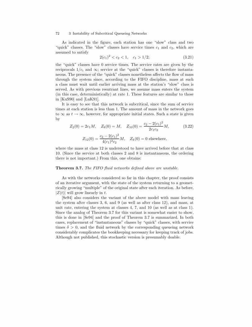
72 3 Instability of Subcritical Queueing Networks
As indicated in the figure, each station has one “slow” class and two“quick” classes. The “slow” classes have service times c1 and c2, which areassumed to satisfy
2(c1)2 < c2 < 1, c1 > 1/2; (3.21)
the “quick” classes have 0 service times. The service rates are given by thereciprocals 1/ci and ∞; service at the “quick” classes is therefore instanta-neous. The presence of the “quick” classes nonetheless affects the flow of massthrough the system since, according to the FIFO discipline, mass at sucha class must wait until earlier arriving mass at the station’s “slow” class isserved. As with previous reentrant lines, we assume mass enters the system(in this case, deterministically) at rate 1. These features are similar to thosein [KuS90] and [LuK91].
It is easy to see that this network is subcritical, since the sum of servicetimes at each station is less than 1. The amount of mass in the network goesto ∞ as t → ∞, however, for appropriate initial states. Such a state is givenby
Z2(0) = 2c1M, Z8(0) = M, Z10(0) =c2 − 2(c1)2
2c1c2M, (3.22)
Z12(0) =c2 − 2(c1)2
4(c1)2c2M, Zk(0) = 0 elsewhere,
where the mass at class 12 is understood to have arrived before that at class10. (Since the service at both classes 2 and 8 is instantaneous, the orderingthere is not important.) From this, one obtains:
Theorem 3.7. The FIFO fluid networks defined above are unstable.
As with the networks considered so far in this chapter, the proof consistsof an iterative argument, with the state of the system returning to a geomet-rically growing “multiple” of the original state after each iteration. As before,|Z(t)| will grow linearly in t.
[Se94] also considers the variant of the above model with mass leavingthe system after classes 3, 6, and 9 (as well as after class 12), and mass, atunit rate, entering the system at classes 4, 7, and 10 (as well as at class 1).Since the analog of Theorem 3.7 for this variant is somewhat easier to show,this is done in [Se94] and the proof of Theorem 3.7 is summarized. In bothcases, replacement of “instantaneous” classes by “quick” classes, with servicetimes δ > 0, and the fluid network by the corresponding queueing networkconsiderably complicates the bookkeeping necessary for keeping track of jobs.Although not published, this stochastic version is presumably doable.

3.2 Examples of Unstable FIFO Networks 73
An unstable FIFO network with quick service times
The examples of unstable subcritical networks given so far all have at leastone class with mean service time greater than 1/2. In each of these examples,it follows that the traffic intensity ρj is greater than 1/2 at some station j.What happens when ρj is uniformly small at all stations? Must all such FIFOqueueing networks be stable? The following example from [Br94b] shows thisis not the case.
Jobs are assumed to follow one of two nearly identical routes, the “up-per”and “lower” routes, at the end of which they exit from the system. Asillustrated in (3.23), there are J stations along each route. (Because of spaceconsiderations, we label only the stations but not the classes along each route.)
→ 1 → 2 → . . . → 2 → 3 → . . . → 3 → . . . → J → . . . → J →(3.23)
→ 1 → 1 → 2 → . . . → 2 → 3 → . . . → 3 → . . . → J → . . . → J → 1 →
Jobs are assumed to enter each route at rate 1/2. Along each route, thestations j = 2, . . . , J are each visited seven times; at each such station, thefirst visit is “slow” and the remaining six visits are “quick”. Only the visitto station 1 at the end of the lower route is “slow”; the three earlier visits tostation 1 along both routes are “quick”.
We now give a precise description of the network depicted in (3.23). Weemploy the notation (i, j, k) for a class, with i = u, $ denoting its route,j = 1, . . . , J denoting its station, and k denoting the order this class is visited,among classes of its station along this route. One has k = 1, . . . , 7 for j =2, . . . , J ; k = 1 for i = u and j = 1; and k = 1, 2, 3 for i = $ and j = 1. The twotypes of jobs are assumed to enter the system according to independent rate-1/2 Poisson processes. Service times of jobs are independent and exponentiallydistributed, with means
c at (i, j, 1), for i = u, $ and j = 2, . . . , J,
c at ($, 1, 3), (3.24)δ at (i, j, k), for i = u, $, j = 2, . . . , J and k = 2, . . . , 7,
δ at (u, 1, 1), ($, 1, 1) and ($, 1, 2).
We assume that
0 < c ≤ 1100
, 0 < δ ≤ c8, J = ,2c−1 log(c−1)-. (3.25)
Each of the stations 2, . . . , J therefore has one comparatively slow and six(very) quick classes for each type of job; station 1 has only the single quickclass for the upper jobs, and two quick classes and one slow class for lowerjobs. The choice of parameters is made for technical reasons. (The coefficient2 in the definition of J has been chosen so that (1 − c)−J ∼ c−2. The bound

74 3 Instability of Subcritical Queueing Networks
c ≤ 1/100 is somewhat arbitrary.) One can think of this family of networksas being constructed by piecing together J copies of the middle section ofnetworks of the type in (3.10). (We only need K = 7 here, although K ≥ 7can instead be used.)
Under (3.25),
ρj ≤ c + 6δ ≤ 2c for j = 1, . . . , J.
So, by choosing c small, the traffic intensity can be chosen as small as desiredfor each j. Nonetheless, the following is true.
Theorem 3.8. FIFO queueing networks with the routing in (3.23) and meanservice times in (3.24)-(3.25) are unstable.
To demonstrate Theorem 3.8, one employs an appropriate analog of Propo-sition 3.6. One can then argue exactly the same way as immediately afterProposition 3.6 to finish the proof of Theorem 3.8. The spirit of the proofof this analog is similar to that of Proposition 3.6, although details are moreinvolved. The purpose of the upper jobs is solely to restrict the flow of thelower jobs. Because of the multiple stations employed here, the same reasoningthat shows, in the previous network, that the main body of jobs remains closetogether, cannot be applied directly. However, with the control resulting fromthe upper jobs, one can analyze the flow of lower jobs much as was done inProposition 3.6. For more details, the reader is referred to [Br94b] or [Br95].Presumably, the analog of Theorem 3.8 holds for an appropriate reentrantline, most likely with a route corresponding to that of the lower jobs in (3.23),although the reasoning given in [Br94b] no longer suffices.
Theorem 3.8 has the following interesting consequence. One can compareany FIFO queueing network satisfying (3.24)-(3.25) with the network thatis obtained from it by replacing (3.24) with the assumption that the meanservice time mi,j,k = c at every class. The lengths of the mean service timesfor the new network are, of course, everywhere at least as great as those ofthe original network. This new network is a subcritical FIFO network of Kellytype with ρj ≤ 7c for all j. Such a FIFO network has a stationary distributionthat is given by (2.4) and (2.9). In particular, the stationary probability ofthere being n jobs at a given station is at most (1 − 7c)(7c)n, n ≥ 1, whichmeans that the network is in fact “very stable” for small c. This comparisonshows that decreasing the mean service times within a queueing network mayresult in making it unstable.
At present, there is a lack of general criteria for the stability of FIFO queue-ing networks. The difficulties are illustrated by the previous examples. Theydo not, however, rule out two possible criteria for stability. Set mmin
j (mmaxj )
equal to the minimum (maximum) over all mk, k ∈ C(j), where j is fixed,and set mR
j = mminj /mmax
j .The first criterion is that, for given mR > 0, there exists an r > 0, so that
if a FIFO network satisfies mRj ≥ mR and ρj ≤ r, for all j, then it is stable.

3.3 Other Examples of Unstable Networks 75
The second criterion is that, for given r < 1, there exists an mR < 1, so thatif a FIFO network satisfies mR
j ≥ mR and ρj ≤ r, for all j, then it is stable.According to the first criterion, if the mean service times at a given station
are not too different, then small enough traffic intensities suffice for stabilityindependently of the specific structure of the network. Similarly, according tothe second criterion, a subcritical network, with ρj ≤ 1− ε for all j and givenε > 0, is stable as long as the ratios mR
j are close enough to 1. Networks ofKelly type, with mR
j ≡ 1, make up the limiting case in the latter scenerio.Note that the first criterion becomes elementary if the routing of the networkis instead specified before r is chosen, since the total number of classes is thenfixed. In that setting, r can be chosen small enough so that Σjρj < 1, whichimplies the network is stable by the example at the end of Section 4.4. Noprogress has been made toward justifying or disproving these criteria.
3.3 Other Examples of Unstable Networks
In the previous two sections, we have given a number of examples of subcriticalqueueing networks that are unstable. Here, we give several other examples ofunstable queueing networks. In some of these cases, more can be said aboutthe region of stability as the traffic intensity ρ varies.
The first example we consider is from [DaWe96]. It consists of a subcriticalSBP reentrant line of Kelly type that is unstable. (Recall that a network is ofKelly type if all classes at a given station have the same mean service time.)This contrasts, of course, with the stability of FIFO networks of Kelly typethat was shown in Chapter 2.
The second example is from [Du97]. It exhibits a family of SBP networksfor which the region of stability is nonmonotone in the parameter ρ, behaviorthat is shared with the last example in the previous section. The region ofstability is, moreover, explicitly calculated and is not convex.
The last example is from [BaBo99]. The family of networks given there isFIFO, but with the added feature that the number of jobs on one of the givenroutes in the network is bounded at any given time. The region of stabilityhere is also calculated explicitly and is neither monotone nor convex. Theboundary is, moreover, self-similar around one of its boundary points.
An unstable network of Kelly type
In contrast to FIFO networks, it is not sufficient for a subcritical queueingnetwork to be of Kelly type for it to be stable. It is not difficult to produce areentrant line, with an appropriate SBP discipline, that exhibits this behavior.Such an example is provided in [DaWe96].
This example consists of two stations, with each station being visited threetimes, and is depicted in Fig 3.5. The priority scheme is (6,5,1) at station 1and (3,2,4) at station 2, e.g., the last class visited at station 1 has the highest

76 3 Instability of Subcritical Queueing Networks
priority and the first class visited there has the lowest priority. The disciplineis preemptive. We assume, as usual, that jobs enter the network according to arate-1 Poisson process. We also assume that the service times are exponentiallydistributed, with mean 0.3 at each class. The network is clearly subcritical,with ρ = (.9, .9).
j = 1 j = 2
k = 2
k = 3
k = 4
k = 1
k = 6
k = 5
0.3
0.3
0.3
0.3
0.3
0.3
Fig. 3.5. This reentrant line has priority scheme (6,5,1) at station 1 and (3,2,4) atstation 2. All service times have mean 0.3.
Theorem 3.9. The static priority reentrant line of Kelly type in Figure 3.5is unstable.
We motivate Theorem 3.9 by comparing the evolution of the reentrant linethere with the evolution of the Lu-Kumar network; a rigorous argument canbe given by mimicking the proof of Theorem 3.2. First note that if one both“combines” the last two classes of station 1, k = 5 and k = 6, into a singleclass and “combines” the first two classes of station 2, k = 2 and k = 3, intoa single class, one obtains the four-class reentrant line whose route and meanservice times are given in Figure 3.6.
We assign to the classes of the new reentrant line the same priority schemeas in the Lu-Kumar network, with k′ = 4 having priority over k′ = 1, and=k′ = 2 having priority over k′ = 3. Adding the service times at the combinedclasses produces service times having gamma distributions with means 0.6, inboth cases.
Some thought shows that this new network is a natural “projection” of thatin Figure 3.5, in the sense that there is a pathwise correspondence betweenthe evolution of jobs in the two networks, with the understanding that jobsat k = 5 and k = 6, respectively at k = 2 and k = 3, in the old networkare combined into k′ = 4, respectively k′ = 2, in the new network. Thiscorrespondence relies on the assigned priority scheme for the old network:both classes 5 and 6, respectively classes 2 and 3, have higher priority thanclass 1, respectively class 4, and so the information lost in the projection isimmaterial in assigning the priority of service to jobs in the combined class

3.3 Other Examples of Unstable Networks 77
k′ = 1 k′ = 2
k′ = 3k′ = 4
0.3
0.30.6
0.6
Fig. 3.6. “Combining” classes k = 5 and k = 6 into a single class and k = 2 andk = 3 into a single class produces this reentrant line, with the above mean servicetimes.
with respect to the other remaining class. Moreover, since class 6 has higherpriority than class 5 and class 3 has higher priority than class 2 in the oldnetwork, jobs currently in service in the new network at class 4 and at class 2will not be preempted in the middle of their service by other jobs there. Thisallows us to maintain the pathwise correspondence between jobs in the twonetworks.
Because of the above relationship between the two networks, instabilityof one network implies instability of the other. The projected network is thesame as the Lu-Kumar network in Theorem 3.2, except that the exponentiallydistributed service times at classes 2 and 4 are replaced by service timeswith gamma distributions there, each with mean 0.6. As mentioned after thestatement of Theorem 3.2, the assumption that service times are exponentialis not needed there, if one is willing to allow a more general state space. Since0.6 > 0.5, as required in the theorem, it will follow that the network in Figure3.6 is unstable. One can also show Theorem 3.9 without referencing Theorem3.2, but instead by mimicking its proof; the setup there has some similaritywith the “method of stages” employed in Section 2.4.
Two examples with nonconvex regions of stability
The first example is an SBP queueing network from [Du97]. As in theRybko-Stolyar network of Section 3.1, jobs travel along one of two routesthat are oriented in opposite directions. In the present setting, there are threestations having two classes each, with the classes labelled according to theroute and position along the route, as in Figure 3.7. Jobs of the second routeare assumed to have priority over jobs of the first route at each of the firsttwo stations, with this being reversed at the third station. The discipline ispreemptive. Jobs enter the routes according to independent rate-αk Poissonprocesses, i = 1, 2, and have independent exponentially distributed servicetimes with means mi,k.
Consider the functions F1(ρ), F2(ρ), and F3(ρ) defined by
F1(ρ) = (ρ1,1 + ρ2,3 − 1) ∨ (ρ1,2 + ρ2,2 − 1) ∨ (ρ1,3 + ρ2,1 − 1) ∨ (ρ1,3 + ρ2,2 − 1),F2(ρ) = (ρ1,3 + ρ2,3 − 1)(1 − ρ1,2 − ρ2,2) − (ρ1,2 + ρ2,3 − 1)(1 − ρ1,3 − ρ2,1),F3(ρ) = (ρ1,3 + ρ2,3 − 1) ∧ [(ρ1,3 − ρ1,2) ∨ F2(ρ)],

78 3 Instability of Subcritical Queueing Networks
j = 1 j = 2 j = 3
(1, 1)
(2, 3)
(1, 2)
(2, 2)
(1, 3)
(2, 1)
Fig. 3.7. The priority scheme favors the classes (2,3), (2,2), and (1,3), respectively,at the stations 1, 2, and 3.
where ρi,k = αkmi,k. (Recall that a ∨ b = max(a, b) and a ∧ b = min(a, b)).Also, set F (ρ) = F1(ρ) ∨ F3(ρ). The regions of stability/instability for thenetwork can be explicitly written in terms of these functions.
Theorem 3.10. The SBP network in Figure 3.7 is stable if F (ρ) < 0 andunstable if F (ρ) > 0.
The reader should not focus too much on the specifics of F (ρ). For ourpurposes, it is enough to observe that the regions of stability/instability areexplicit and are considerably more complicated for this relatively elementarynetwork than for either the Lu-Kumar or Rybko-Stolyar network. Moreover,(a) the region of stability F (ρ) < 0 is not convex and (b) stability is notmonotone in ρ, i.e., one can find ρ < ρ′ with F (ρ) > 0 and F (ρ′) < 0. Bothproperties follow from Theorem 3.10 by setting ρ1,1 = ρ2,2, ρ1,2 = ρ2,3, andρ1,3 = ρ2,1, and restricting F (ρ) < 0 to this three dimensional subspace. Slicesof this region at fixed values of ρ1,1 can then be analyzed. As a quick checkon the consistency of the instability condition F (ρ) > 0, note that F1(ρ) > 0if any of the three stations is supercritical.
In order to show both directions of Theorem 3.10, [Du97] employs er-godic/transience criteria developed in [MaM81] for reflected random walkson Zd
+,0. Motivation for the definition of F (ρ) is provided by fluid equationsthat correspond to the original network. These equations are related to fluidmodels, which will be studied in the next chapter.
The second example we discuss is from [BaB99] and examines a family ofnetworks consisting of a single route with controlled jobs and multiple trans-verse routes with cross jobs. ([BaB99] employs the terms controlled customersand cross customers.) Controlled jobs moving along their route visit each ofthe J stations in the network once; the cross jobs each visit only a single sta-tion before exiting the network. No more than L controlled jobs are allowedin the network at a given time; when there are more than L such jobs, theexcess jobs wait at an outside buffer until a controlled job leaves the network,at which point the first such job enters the network. There is no such restric-tion on cross jobs. (See Figure 3.8.) All jobs are served according to the FIFOdiscipline at each station. These networks can be thought of as a simple modelwith window flow control for packet-switched communication networks.

3.3 Other Examples of Unstable Networks 79
. . .
Fig. 3.8. The controlled jobs move horizontally and the cross jobs move vertically.The number of controlled jobs in the network at a given time is restricted, withexcess controlled jobs required to wait at the outside buffer on the left. There arecurrently 3 jobs waiting at the outside buffer.
Detailed analysis of such a system is possible under certain restrictive as-sumptions. Set J = 2 and L = 1, and assume that the service times for all jobs(both controlled and cross) are deterministic and take value 1. Also, assumethat the interarrival times of the cross jobs at station 1 are deterministic andtake value τ , with τ ≥ 1, and that there are never any cross jobs at station2. There are only minimal assumptions on the interarrival times for the con-trolled jobs, namely that they define a stationary and ergodic point processwith some intensity λ.
On account of the outside control on jobs, this network differs from theother examples considered in this chapter. Also, because of the deterministicaspects of this model, it is more appropriate to weaken the definition of stableused elsewhere, and only require here that the model support a stationaryprocess (that need not be ergodic). The definition of unstable remains thesame as before.
This network is interesting because of how its region of stability dependson τ . For fixed τ , stability is monotone in the parameter λ, and does nototherwise depend on the arrival process for the controlled jobs; there is a λ sothat for λ < λ, the network is stable, while for λ > λ, it is unstable. In Figure3.9, λ is graphed as a function of λ1 = τ−1, with the heavy line being boththe graph of λ and the boundary between the stable and unstable regions.
As in the example in Figure 3.7, the region of stability of the networkis not convex. Also, as in previous examples, it is not monotone. (This non-monotonicity is in terms of the intensity of the cross traffic, though, insteadof in terms of the mean service times, as in the previous examples.) Moreover,the graph of λ is self-similar around (0, 1
2 ), as is indicated in Figure 3.9. Anopen question is what part of this behavior remains when the deterministicinterarrival and service times in the model are randomized.
Two other families of networks with nonmonotone regions of stability aregiven in[Br98a] and [DaHV99]. In both cases, decreasing the service timedistributions can destabilize the network. In [Br98a], this is done by showinga network can be stabilized by inserting a single class station immediatelybefore the visit to each class. (Related deterministic work was done in [Hu94].)

80 3 Instability of Subcritical Queueing Networks
In [DaHV99], this is done in the context of global stability, which is discussedin Section 5.4.
14
15
13
16
17
18
12 1
λ1
λ
1
0
12
Fig. 3.9. This is the graph of λ as a function of λ1 = τ−1, which is the boundarybetween the stable and unstable regions. (The heavy line is the graph of λ; thedotted lines help one track the piecewise linear increments of λ.)The graph of λ isself-similar around (0, 1
2 ). (Example reprinted from [BaB99] with permission fromBaltzer.)

4
Stability of Queueing Networks
In Chapter 2, we demonstrated the stability of several families of queueingnetworks by explicitly computing their stationary distributions. For queue-ing networks with other disciplines, or with nonexponential interarrival andservice times, one cannot expect such explicit expressions. So, in order to in-vestigate the stability of more general queueing networks, another approach isneeded. Such an approach should be more qualitative and less computationalin nature.
The approach we employ in this chapter to study the stability of queueingnetworks employs fluid limits and fluid models. Fluid models were discussedbriefly in Section 1.3; we will examine both fluid limits and fluid models indetail here. Employing these tools, one can reduce the study of queueingnetworks to their simpler deterministic analogs. The basic theory is givenhere; applications will be given in Chapter 5.
In the next several paragraphs, we give some background on previous re-sults on the stability of queueing networks. We recall that a queueing networkis defined to be stable if its underlying Markov process is positive Harris re-current. As mentioned earlier, when the state space is countable and all statescommunicate, this definition reduces to the usual definition of positive recur-rence. Results in earlier works are typically stated within this more restrictiveframework.
Interest in whether general families of queueing networks are stable hasdeveloped since the 1980’s. Most early work was restricted to single classnetworks (see, e.g., [Bo86], [Si90], [BaF94], [ChTK94], and [MeD94]). Workon multiclass networks usually dealt with deterministic systems, with eitherdiscrete or continuous job mass (see, e.g., [PeK89], [KuS90], [LuK91], and[Ku93]); examples of both types of systems were given in Chapter 3. “Stabil-ity” for such deterministic systems was shown in various cases in the aboveliterature, with stability, in this context, typically meaning that the quantityof job mass in the system converges to 0 or remains bounded over time. As inthe stochastic setting, ρ < e is the natural requirement for stability.

82 4 Stability of Queueing Networks
Examples of unstable deterministic networks, with ρ < e, were given in[KuS90] and [LuK91]. An example of an unstable network in the stochas-tic setting was given in [RyS92]; these and other examples were discussedin Chapter 3. Such examples illustrate the importance of the discipline indetermining whether a queueing network is stable.
It has long been believed that queueing networks should be stable undergeneral assumptions. Inclusive conditions for stability are not known (andlikely do not exist). Instead, stability is typically shown in the context of aspecific discipline, under ρ < e and perhaps other constraints. The approachwe present in this chapter, using fluid limits and fluid models, reduces thestudy of such problems to a simpler, deterministic setting.
The foundation for this approach was given in [RyS92]. For a two stationFIFO queueing network, with the same routing as in Figure 3.2 and withexponential interarrival and service times, the authors showed stability whenρ < e. Their argument involved showing the “stability” of solutions of a re-lated deterministic system, and showing that rescaled solutions of the randomsystem remain close to those of the deterministic system. As pointed out in[RyS92], this procedure is, in principle, quite general in nature. However, forall but the simplest systems, technical problems arise when comparing solu-tions of the random and deterministic systems.
Independently, [St95] and [Da95] developed criteria for the stability ofqueueing networks, in terms of the stability of limits of rescaled solutions ofthe network. (In the terminology of this chapter, [St95] used fluid limits and[Da95] used both fluid limits and fluid models.) [St95] assumed exponentialdistributions for the interarrival and service times; [Da95] considered moregeneral distributions, but at the price of requiring the use of Markov processeswith general state space. Applications illustrating this approach are given in[Da95].
The material in this chapter is based on the approach taken in [Da95]. Themain theorem of the chapter, Theorem 4.16, corresponds to Theorem 4.2 in[Da95]. Our approach here is a modification of that in [Br98a]. Care has beentaken to give a detailed presentation of the material, including that cited in[Da95]. As a consequence, the chapter is quite long; in the remainder of theintroduction, we summarize its contents.
Summary of chapter
Chapter 4 consists of five sections. In Section 4.1, we present the founda-tions for the Markov processes we will need. We first give a detailed construc-tion of the underlying Markov process for an HL queueing network. We nextsummarize relevant results from general Markov process theory. The thirdpart of the section defines Harris recurrence and positive Harris recurrence,and gives an alternative formulation, in Theorem 4.1, that we will use.
We recall that a queueing network is e-stable, if its underlying Markovprocess is ergodic. In the last part of Section 4.1, we give general conditions

4 Stability of Queueing Networks 83
under which ergodicity holds. At the end of Section 4.4, we will use this togive criteria under which a queueing network is e-stable. In the continuoustime, countable state space setting, positive Harris recurrence and ergodicityare equivalent.
Much of the material in Section 4.1 may be unfamiliar to readers. We pointout that concepts such as positive Harris recurrent and petite are motivated bysimilar concepts in both the discrete time and countable state space settings.Various proofs either rely on, or are motivated by, similar results in thesesettings. Those readers who are interested in further background can refer toSection 4.5, which serves as an appendix to this section.
When the interarrival and service times are exponentially distributed, theunderlying Markov process of the queueing network can, for many disciplines,be constructed on a countable state space. This considerably simplifies thepreparation that is required to derive Theorem 4.16. In particular, one doesnot require the general machinery that is introduced in Section 4.1. For readerswishing such a “shortcut”, we present a summary, at the end of the differentsections, saying how the general approach presented here can be modified. (InSection 4.4, the summary is instead presented after Theorem 4.16.) Here inthe introduction, we will also point out these shortcuts.
In Section 4.2, we present two results on bounded sets that we will needlater on. The first, Proposition 4.6, is a variant of Foster’s Criterion, whichwe refer to as the Multiplicative Foster’s Criterion. The main condition isthat, off of a bounded set, the Markov process X(·) have a uniformly negativedrift on an appropriate time scale. One also requires that the bounded set beeither petite or uniformly small, which are defined in Section 4.1. (In essence,petite means that all sets, weighted according to some measure, are “equallyaccessible” from any point in the petite set. Uniformly small is a somewhatstronger concept that is defined similarly.) One concludes that X(·) is posi-tive Harris recurrent when the condition petite is assumed and ergodic whenuniformly small is assumed. In the countable state space setting, the petiteand uniformly small conditions can be dropped, since the empty state will beequally accessible from all points in the bounded set. Moreover, Theorem 4.1,from Section 4.1, is not needed for the proof of the Multiplicative Foster’sCriterion in the countable state space setting.
The other result from Section 4.2, that we will need later, is Proposition4.7. It says that when the interarrival times of a queueing network satisfy cer-tain conditions, bounded sets will be uniformly small, and hence also petite;this enables us to employ the Multiplicative Foster’s Criterion. The proposi-tion is not needed in the countable state space setting.
Section 4.3 introduces fluid models and fluid limits. The first part of thesection recalls the queueing network equations that were discussed briefly inSection 1.3; we provide more detail here. Fluid model equations are the deter-ministic analogs of the queueing network equations. They were also discussedbriefly in Section 1.3; we provide further detail in the second part of Section4.3. There, emphasis is placed on the basic fluid model equations, which are

84 4 Stability of Queueing Networks
the fluid model equations that do not depend on a specific discipline. Proposi-tion 4.11, in the subsection, presents several elementary results on fluid modelsthat will be used later. Two examples are given that illustrate nonuniquenessof fluid model solutions and instability when the system is subcritical.
Fluid limits are introduced in the last part of Section 4.3. They provide arigorous connection between the queueing network and fluid model equations,with the latter being satisfied by limits of solutions of the former, under a“law of large numbers” scaling. Variants of fluid limits have been present inthe literature at least since [Ne82] (see also [ChM91]).
The use of fluid limits, as in Proposition 4.12 of this section, makes therelationship between queueing network and fluid model equations precise. Theconnection between queueing network and fluid model equations will be impor-tant in Section 4.4, where we use the stability of fluid models (and, indirectly,of fluid limits) to show the stability of queueing networks. The approach takenin this section remains essentially the same when employed in the countablestate space setting.
In Section 4.4, we demonstrate Theorem 4.16, which is the main result onthe stability of queueing networks. As assumptions, one needs bounded sets tobe petite and the fluid limits to be stable. Proposition 4.7, from Section 4.2,gives sufficient conditions for the former property to hold. The MultiplicativeFoster’s Criterion will be used, in conjunction with Proposition 4.7 and thebounds given in Section 4.4, to demonstrate Theorem 4.16. The work requiredfor this simplifies considerably in the countable state space setting.
After the theorem, we provide various commentary, such as on modifica-tions of its assumptions. One such modification, substituting uniformly smallfor petite, suffices for the stronger conclusion that the network is e-stable. Theresult, Theorem 4.17, follows by applying Theorem 4.3 from Section 4.1, andotherwise reasoning as in the proof of Theorem 4.16. As mentioned earlier,in the continuous time, countable state space setting, stability and e-stabilityare equivalent.
4.1 Some Markov Process Background
In this section, we first introduce the Markov processes that are associatedwith HL queueing networks. We next consider these Markov processes inan abstract setting, in which we define positive Harris recurrence. We thenpresent a useful alternative characterization of positive Harris recurrencewhich will be applied to queueing networks in the following sections. Some ofthe background for this material is relegated to Section 4.5, which serves asan appendix to this section.
We note that in the countable state space setting, the material that isneeded from this section is minimal. The construction of the Markov processsimplifies, since sample paths are piecewise constant with finite jump rates.

4.1 Some Markov Process Background 85
Moreover, standard recurrence concepts from Markov chain theory apply, andso the discussion of Harris recurrence that is given here is not needed. Moredetail is given at the end of the section.
Definition of the Markov process
In this subsection, we give a careful construction of the Markov processthat is associated with a given HL queueing network. Readers are encouragedto consider this material, but those who are not interested in the technicaldetails should feel free to skip ahead to the next subsection. If the reader doesso, he/she should keep in mind that we are defining continuous time Markovprocesses, on an appropriate space and with dynamics that correspond to thequeueing networks of interest. One should note the “norm” |x| of a state x,which is given in (4.3): it is the sum of components corresponding to thequeue lengths, and residual interarrival and service times of the state. It willbe employed later on in the chapter.
We begin by defining the state space (S, S ) of the Markov process. In orderto motivate the different components of states of the space, we will repeatedlyallude to the various queueing network quantities they will correspond to.
The state of the Markov process, at any time, will be given by a pointx = (y, r), where
y ∈ (Z × R)∞ × R|A| × RK and r ∈ RK , (4.1)
and the coordinates are subject to appropriate positivity restrictions. Recallthat A is the set of classes at which external arrivals are allowed. It is assumedthat only a finite number of the pairs of coordinates of (Z×R)∞, indexed byi, are nonzero. For such a pair, the first coordinate ki, ki = 1, . . . , K, is tobe interpreted as the current class of a job in the network, with the secondcoordinate si, si ≥ 0, measuring how long ago the job entered this class, wheresi is given in descending order. The job with the largest second coordinate,among those with first coordinate k, is thus the first or “oldest” job of class k.(For “ties” where two or more pairs have the same second coordinate, orderthe job with the smaller k coordinate first.)
We denote by z = (z1, . . . , zK) the number of jobs in each class, and set|z| =
∑Kk=1 zk. The vector r is assumed to have coordinates rk ∈ [0, 1], k =
1, . . . , K, with rk = 0, for zk = 0, and which sum to 1 over each nonemptystation j. For each nonempty class k, the coordinate rk is to be interpretedas the service rate of the oldest job of this class, with other jobs receiving noservice. (This is the HL property.) The coordinates uk, uk > 0, of R|A| areto be interpreted as the residual interarrival times for classes k, with k ∈ A.(That is, uk is the remaining time before the next arrival at k of a job fromoutside the network.) The coordinates vk of RK , for the y component, are theresidual service times for the oldest job at each class k, k = 1, . . . , K, withvk > 0 except when zk = 0, in which case we set vk = 0. We denote by u andv the corresponding vectors, and set |u| =
∑k∈A |uk| and |v| =
∑Kk=1 |vk|.

86 4 Stability of Queueing Networks
We denote by S the space given by (4.1) and the above restrictions on thecoordinates. We wish to specify a metric on S. For this, it is convenient todenote by ri the service rate assigned to the ith job, i = 1, . . . , |z|. The metricis defined by adding up the contribution of each of the coordinates in (4.1),after taking differences for individual terms. Specifically, for x, x′ ∈ S, withcorresponding coordinates as denoted above, we set
d(x, x′) =∞∑
i=1
((|ki − k′i| + |si − s′i| + |ri − r′i|) ∧ 1) (4.2)
+∑
k∈A|uk − u′
k| +K∑
k=1
|vk − v′k|.
For most purposes, we will not require the full metric, but just the associated“norm” | · |, with
|x| = |z| + |u| + |v|. (4.3)
(|x| can be interpreted as the distance from x to the “origin”, which is not inthe space, however.) Note that |x| is continuous as a function of x. We alsoequip S with the standard Borel σ-algebra inherited from the metric, whichwe denote by S .
Since only a finite number of the coordinate pairs in (Z×R)∞ are nonzero,it is not difficult to see that the metric d(·, ·) is separable. It is also locallycompact; with a bit of work, one can show this by showing that an openball around a point x is homeomorphic to a finite product of intervals of theform (0, 1) and [0, 1). (Half-closed intervals are needed when either si = 0,si = si′ for some i '= i′, or the coordinates rk of r corresponding to a givenstation j are on the boundary of the simplex
∑k∈C(j) rk = 1.) The metric
is not complete, since one can choose Cauchy sequences xn, with un → 0 orvn → 0 as n → ∞, that have no limit in S. It is, however, homeomorphic tothe complete metric d′(·, ·) obtained by replacing the term
∑k∈A |uk − u′
k| in(4.2) by
∑
k∈A
(|uk − u′
k| +∣∣∣∣
1uk
− 1u′
k
∣∣∣∣ ∧ 1)
,
and∑k
k=1 |vk − v′k| by the analogous term (where we set 10 − 1
0 = 0). Weprefer to work with the simpler metric d(·, ·), since we will not require S tobe complete.
We now formally define the Markov process underlying an HL queueingnetwork as the stochastic process X(t), t ≥ 0, on S that undergoes the follow-ing evolution. We continue to use the same suggestive queueing vocabularythat was employed in motivating the construction of S.
We set X(t) = (Y (t), R(t)), with Y (t) and R(t) taking values y and r asin (4.1). (The coordinates si of y are allowed to exceed t, and so jobs may,in effect, arrive before time 0.) The evolution of X(t), in between arrivalsand departures of jobs at classes, is given by the service rates Rk(t), which

4.1 Some Markov Process Background 87
are constant over such intervals. Upon an arrival or departure somewhere inthe network at time t, the stochastic process is continued by assigning newservice rates R(t) = f(Y (t)), where f is a measurable function. The choice off corresponds to the discipline of the corresponding HL queueing network.
In order to describe the transition of X(t) upon the arrival or departure ofa job at a class, we introduce the sequences of positive i.i.d. random variablesξk(i), k ∈ A, and γk(i), k = 1, . . . , K, with i = 1, 2, 3, . . ., which correspond tothe interarrival and service times of the queueing network. We will also needthe sequence of i.i.d. random vectors φk(i), i = 1, 2, 3, . . ., with φk(i) = e!for some $ = 1, . . . , K or φk(i) = 0, which give the routing of a job uponcompletion of its service at a class. (Here, e! ∈ RK is the unit vector inthe positive $ direction.) We assume the sequences ξ, γ, and φ are mutuallyindependent. These sequences, together with the function f and the initialstate x, will determine the evolution of X(·) for all times along each samplepath.
The process X(t) can be constructed inductively as follows. At times tbetween arrivals and departures, R(t) = r gives the rate of decrease of eachcomponent of the residual service time vector V (t) = v. When Vk(t−) = 0occurs for some k, service at k for the oldest job of that class is assumed tobe completed, with the job being routed to another class $, if φk(i) = e!,and leaving the network, if φk(i) = 0, where φk(i − 1) is the previous routingvector applied at k. When this occurs, one sets Vk(t) = γk(i) if class k is thennonempty, and sets Vk(t) = 0, if k is empty. Until a job leaves its class, its ageSi(t) = si continues to increase at rate 1. (The label i of a job will typicallychange as it moves from one class to another.)
The components of the residual interarrival time vector U(t) = u alwaysdecrease at rate 1 until hitting 0. At the time t for which this occurs at agiven k, one includes the pair (k, 0) in the state Y (t) and sets U(t) = ξk(i),where i is the index of the first unused interarrival time at k at time t. If theclass k is empty at time t−, and hence Vk(t−) = 0, one sets Vk(t) = γk(i′),where i′ is the index of the first unused service time at time t.
In various cases, the state space S can be simplified for queueing networkswith specific HL disciplines, or specific interarrival and service time distribu-tions. For instance, when the interarrival and service times are exponentiallydistributed, one can drop the u and v coordinates from the description of thestate (unless r is chosen to depend on them).
Preemptive static buffer priority disciplines were introduced in Chapter 1.Such networks are HL, with ri = 1 automatically holding for the oldest job ofthe highest ranked nonempty class at each station. One can therefore drop theage of jobs from the state space descriptor. As mentioned above, the residualinterarrival and service times can also be dropped from the descriptor whenthe corresponding variables are exponentially distributed. The state space canthen be reduced to points in ZK with nonnegative coordinates, if one implicitlyassumes the given priority scheme that orders classes at each station, sinceone is able to drop the coordinate r that governs service.

88 4 Stability of Queueing Networks
Networks with the FIFO discipline are also HL, since the oldest job at astation is always served first. If one chooses, one can drop the age of jobs fromthe state space descriptor, by instead ordering the ages at each station; onecan also drop the coordinate r. As before, coordinates can also be eliminatedwhen the interarrival and service times are exponentially distributed. Theresulting state space will then be countable.
The state space S is large enough to contain the information needed forthe queueing networks we will investigate. It can, however, be modified if onehas other applications in mind. For instance, a state space descriptor for howlong ago a job entered the network can be appended. This is needed for theFISFO networks mentioned briefly in Section 1.2 (see, e.g., [Br01]). Also, onecan associate with each job in a class a residual service time, instead of withjust the class itself (see, e.g. [Wi98b]). The definitions (4.2) and (4.3) thenneed to be modified accordingly.
Foundations and terminology
It is not difficult to see that the process X(·) just defined is time homoge-neous and Markov, and that its sample paths are right continuous. AlthoughX(·) is not a jump process, it evolves in a simple manner, having only isolateddiscontinuities and evolving deterministically in between. In particular, aftera jump, the state of X(·) is explicitly known until its next jump, with itsevolution being linear in its coordinates.
The process X(·) is an example of a piecewise-deterministic Markov pro-cess (PDP). Such processes are discussed in [Da84] and [Da93] in detail; wewill rely on the latter in our discussion. In [Da93], PDPs are the more generalfamily of processes whose evolution in between jumps, rather than being lin-ear, is determined by a locally Lipschitz continuous vector field. Also, “killing”at a rate dependent on the position is allowed in [Da93]; after such killing, theprocess jumps according to a given random rule. In our setting, there is nosuch killing. Since, in between jumps, X(·) lives in a subset of S which is home-omorphic to an open ball in Rd, for some d, one can append a “boundary” ∂Sto S, which X(·) hits at a time t− immediately before a jump. For the settingin [Da93], this approach is useful in assigning the jump rule for the process,and it also allows one to define the process on the space DS = DS [0,∞) ofright continuous paths on S with left limits. However, since the process jumpsinstantly upon hitting ∂S, the introduction of ∂S has its own inconveniences.We avoid these complications and just stick with the space S, referring thereader to Sections 24 and 25 of [Da93] for the technical details in the moregeneral setting.
So far, we have not defined the filtration for the process X(·). We let F0t
denote the natural filtration
F0t = σ(X(s), 0 ≤ s ≤ t) (4.4)
and let F0∞ be the σ-algebra generated by F0
t , for t ≥ 0. Rather than employ-ing F0
t and F0∞ directly, we will use appropriate completions. As in [Da93],

4.1 Some Markov Process Background 89
for each initial probability measure µ on S, one can define a measure Pµ onthe sample space corresponding to the process. Letting Fµ
t be the completionof F0
t obtained by including all Pµ-null sets of F0∞, one sets
Ft =⋂
µ
Fµt , (4.5)
and denotes by F∞ the σ-algebra generated by Ft, for t ≥ 0. We henceforthemploy {Ft, t ≥ 0} as the filtration for the process X(·), and use Pµ todenote the corresponding probability measures. This setup is typical of generalMarkov process theory.
In addition to being complete in the sense of (4.5), the family {Ft, t ≥ 0}is right continuous, that is,
Ft = Ft+def=
⋂
ε>0
Ft+ε. (4.6)
Because X(·) is a PDP, this is not difficult to show. (See Theorem 25.3 in[Da93].) The properties (4.5) and (4.6) will be needed shortly for the DebutTheorem and the strong Markov property.
For t ≥ 0, x ∈ S, and A ∈ S , set
P t(x, A) = Px(X(t) ∈ A).
It is shown in [Da93] that P ·(·, ·) is a probability transition kernel on (S, S ).That is, for fixed t and A, P t(·, A) is S -measurable; for fixed t and x, P t(x, ·)defines a probability measure on S; and P s+t = P s ◦ P t, for s, t ≥ 0, definesa semigroup. However, X(·) need not be a Feller process. (Recall that X(·) isa Feller process if, in addition, P t : C(S) → C(S), where C(S) denotes thecontinuous bounded functions on S.) This may be the case even when X(·)corresponds to a queueing network with a FIFO or SBP discipline, since evena small change in the future arrival time of a job may cause it to be servedafter another job instead of before. This can induce a major change in thefuture evolution of X(·), which will imply that for f ∈ C(S), P tf need notbe continuous. Nevertheless, as shown in [Da93], X(·) is strong Markov.
In the next subsection, we will summarize the recurrence theory for Markovprocesses that we will use for queueing networks. Part of the appropriateliterature assumes that these processes are Borel right. The intent there isto employ a well-studied general framework, but this comes at the cost ofimplicitly assuming some familiarity with a technical theory. Such knowledgewill not be relevant for our applications, and so we relegate to Section 4.5 abrief discussion of the material. We summarize it here, noting that for a Borelright process, the σ-algebras satisfy (4.5) and (4.6), the process X(·) is definedon a “reasonable” state space, has a transition semigroup, is right continuous,and the process (f◦X)(·) is right continuous when f is an α-excessive function.The last assumption can be replaced by the strong Markov property.

90 4 Stability of Queueing Networks
Harris recurrence of Markov processes
We discuss here basic criteria for positive recurrence of Markov processeson general state spaces. Since little is a priori assumed about either the statespace or the process itself, one must provide some structure to be able to sayanything of interest. There is a developed theory for the corresponding discretetime Markov processes that goes back to Doeblin (see [Do53] for an account),was developed in [Ha56], and includes contributions by [Or71], [AtN78], and[Nu78] among others. Standard references are [Nu84] and [MeT93d]. The ba-sic approach in the discrete time setting is to formulate conditions that aregeneral, but nonetheless enable one to mimic the machinery for discrete timeMarkov chains. With the aid of resolvents, problems in the continuous timesetting can be reformulated in discrete time, which is the approach we sum-marize here.
Following [MeT93a-93c] and [KaM94], we will assume that the Markovprocesses X(·) are Borel right processes on a locally compact and separa-ble metric state space (S, S ), where S is the Borel σ-algebra generated bythe metric. The process X(·) will have a transition semigroup P t acting onbounded measurable functions, its paths will be right continuous, and theprocess will be strong Markov. (These properties follow from the assumptionthat the processes are Borel right.) When working with discrete time Markovprocesses, we will assume the state space satisfies the same properties.
One wishes to formulate concepts that are the analogs of those for Markovchains, although there will be aspects not present in the countable state spacetheory. For A ∈ S , let
τA = inf{t ≥ 0 : X(t) ∈ A}, ηA =∫ ∞
01{X(t) ∈ A} dt. (4.7)
By the Debut Theorem (see e.g., [Sh88]), τA is a stopping time. A Markovprocess is said to be ϕ-irreducible, for a nontrivial σ-finite measure ϕ on(S, S ), if
ϕ(A) > 0 implies Ex[ηA] > 0 for all x ∈ S; (4.8)
ϕ is called an irreducibility measure.If for some nontrivial σ-finite measure ϕ,
ϕ(A) > 0 implies Px(ηA = ∞) = 1 for all x ∈ S, (4.9)
then X(·) is Harris recurrent. (This definition goes back to [AzKR67].) It isnot difficult to show that it is equivalent to the condition that
ϕ(A) > 0 implies Px(τA < ∞) = 1 for all x ∈ S (4.10)
(see [KaM94] or [MeT93a]), although the choice of ϕ satisfying (4.10) neednot satisfy (4.9). (Consider, for example, the process X(t) = eit on the unitcircle, where ϕ is concentrated at a point.) Both formulations are useful inpractice.

4.1 Some Markov Process Background 91
A σ-finite measure π on (S, S ) satisfying
π(A) = πP t(A) def=∫
P t(x, A)π(dx) for A ∈ S , t ≥ 0, (4.11)
is stationary (or invariant). (Note that the definition does not involve ϕ.) Itwas shown in [Ge79] that if X(·) is Harris recurrent, then there is a uniquestationary measure, up to a constant multiple. (We will discuss this resultin Section 4.5.) If the stationary measure π is finite, it may be normalizedto a probability measure. Harris recurrent processes with such π are positiveHarris recurrent.
The reader should be aware that Harris recurrence and positive Harrisrecurrence have somewhat different implications than recurrence and positiverecurrence, in the countable state space setting. For instance, if ϕ is concen-trated at a point x, then a Markov chain can have x as an absorbing point andstill be positive Harris recurrent. When all states communicate, the definitionsare equivalent.
For discrete time Markov processes, ϕ-irreducibility, Harris recurrence,and positive Harris recurrence are defined by the analogs of (4.8), (4.9) and(4.11). (In this setting, (4.9) and (4.10) are clearly equivalent by the strongMarkov property.) Since there is a wealth of theory available for such Markovprocesses, it is fruitful to be able to translate continuous time problems intothe discrete time setting. This can be done by using the resolvent of thecontinuous time Markov process,
R(x, A) def=∫ ∞
0e−tP t(x, A) dt for x ∈ S, A ∈ S . (4.12)
The Markov process X(n), n = 0, 1, 2, . . ., with one-step transition probabil-ity given by R(·, ·), is known as an R-chain. The R-chain X(·) can also beconstructed directly from X(·) by setting
X(n) = X(σn), n = 0, 1, 2, . . . , (4.13)
where the sequence σ0, σ1,σ2, . . . of random variables, with σ0 = 0, is inde-pendent of X(·) and has i.i.d. mean-1 exponentially distributed increments.(One enriches the sample space so as to include such a sequence.) It is easy tocheck that X(·) is ϕ-irreducible if and only if X(·) is. One can also show thatthe same is true for Harris recurrence and positive Harris recurrence, and thatthe same stationary measure is shared by both processes. The arguments arefairly quick although not immediate; they are given in Section 4.5.
Although the irreducibility measure for a given process X(·) is not unique,there exists a maximal irreducibility measure ψ, i.e., an irreducibility measurefor the process such that ϕ << ψ for any other irreducibility measure ϕ, andsuch that
ψ({x : Px(ηA '= 0) > 0}) = 0 (4.14)

92 4 Stability of Queueing Networks
for ψ(A) = 0 and A ∈ S . (ϕ << ψ means that ϕ is absolutely continuouswith respect to ψ.) The measure ψ is equivalent to
ψ′(A) def=∫
SR(x, A)ϕ′(dx) for x ∈ S, A ∈ S , (4.15)
for any irreducibility measure ϕ′. (That is, ψ << ψ′ and ψ′ << ψ.) Since theexistence of a stationary measure π does not depend on the choice of ϕ, oneis free to assume that ϕ is maximal when addressing such questions.
Maximal irreducibility measures are frequently used in discrete time, where(4.14) and (4.15) are replaced by
ψ({x : Px(τA < ∞) > 0}) = 0 (4.16)
and
ψ′(A) def=∞∑
n=0
2−(n+1)
∫
SPn(x, A)ϕ′(dx) for x ∈ S, A ∈ S . (4.17)
The existence of such a measure ψ and its equivalence to ψ′ in the lattersetting can be found on, e.g., page 88 of [MeT93d]. One can check that (4.14)and (4.15) hold for the process X(·) for a given irreducibility measure ψ ifand only if (4.16) and (4.17) hold for its R-chain X(·), since the right side of(4.17) is equivalent to ψ′′(A) =
∫S P (x, A)ϕ′(dx) in this case.
The above definitions of Harris recurrent and positive Harris recurrent,while elegant, can be difficult to apply in practice. For applications, the fol-lowing alternative formulation involving petite sets is very useful. A nonemptyset A ∈ S is said to be petite if for some fixed probability measure a on (0,∞)and some nontrivial measure ν on (S, S ),
ν(B) ≤∫ ∞
0P t(x, B)a(dt) (4.18)
for all x ∈ A and all B ∈ S ; ν is then called a petite measure. A petite set Ahas the property that each set B is “equally accessible” from all points x ∈ Awith respect to the measure ν. Note that any nonempty measurable subset ofa petite set is also petite. When (4.18) holds, with a being concentrated at asingle point m0, A is said to be small, and ν is called a small measure. Petiteand small sets are defined analogously in the discrete time setting.
LetτA(δ) = inf{t ≥ δ : X(t) ∈ A}.
Theorem 4.1 below gives practical alternative characterizations of Harris re-currence and positive Harris recurrence in terms of petite sets. Versions ofTheorem 4.1 are stated in [MeT93a-c], with that in [MeT93a] being usedhere. Discrete time analogs of the different parts of Theorem 4.1 are known.(See, e.g., [Or71], [Nu84], and [MeT93d].)

4.1 Some Markov Process Background 93
Theorem 4.1. (a) A Markov process X(·) is Harris recurrent if and only ifthere exists a closed petite set A with
Px(τA < ∞) = 1 for all x ∈ S. (4.19)
(b) Suppose the Markov process X(·) is Harris recurrent. Then, X(·) is positiveHarris recurrent if and only if there exists a closed petite set A such that forsome δ > 0 (or, equivalently, for any δ > 0),
supx∈A
Ex[τA(δ)] < ∞. (4.20)
We next make some general comments about Theorem 4.1. We then in-dicate how the theorem will be applied and discuss its proof. More detail onthe proof will be supplied in Section 4.5.
We note that the irreducibility measure ϕ in (4.8) and the measure ν in(4.18) employed in the definitions of Harris recurrence and petite sets aredifferent in general. In [MeT93a], petite sets rather than closed petite setsare employed for Harris recurrence, although closed petite sets are needed forpositive Harris recurrence. We assume the sets are closed in both cases; thissimplifies the proof of one of the steps. We note that the more useful direction(and the only one used in these lectures) is that Harris recurrence and positiveHarris recurrence follow from (4.19) and (4.20), respectively. If one wishes,one can base the definition of Harris recurrence on (4.19), rather than on theirreducibility measure as in (4.9); this is done, for instance, in [As03] (and in[Dur96], in discrete time). This will simplify the work in showing the existenceof a stationary measure.
Theorem 4.1 will prove very useful in conjunction with Section 4.2. There,we will show that for the underlying Markov process X(·) of a queueing net-work,
A = {x : |x| ≤ κ} is a closed small set for each κ > 0, (4.21)
where |x| is given by (4.3), if appropriate conditions hold for the distributionsof the interarrival times for the queueing network. In Section 4.4, we willshow that the conditions (4.19) and (4.20) in the theorem will follow from thestability of the associated fluid limits, which are introduced in Section 4.3.
We next briefly discuss the proof of Theorem 4.1. The demonstration thatX(·) is Harris recurrent if (4.19) holds is elementary, if one sets ϕ = ν. We sum-marize the argument here. Note that X(τA) ∈ A, since A is closed. Startingfrom any x ∈ S and applying the strong Markov property, one can thereforeshow that by a large enough fixed time T (depending on x), X(·) will, withat least a given positive probability that depends on A, hit a specified set Bwith ν(B) > 0. Repetition of this reasoning, using appropriate random timesTn which depend on X(Tn−1), will imply that the probability B has not beenhit after n iterations decreases exponentially quickly in n. This implies (4.10),

94 4 Stability of Queueing Networks
and hence that X(·) is Harris recurrent. ([MeT93a] gives a different argumentthat does not assume A is closed.)
The other direction in Part (a), and both directions in Part (b) of Theo-rem 4.1, require work. In Section 4.5, we will present a summary of the proofs.We will state there a discrete time analog of Theorem 4.1 and indicate howTheorem 4.1 can be shown using this, and the correspondence mentioned ear-lier between Harris recurrence, positive Harris recurrence, and the stationarymeasures for the Markov process and its R-chain. We will also provide a sum-mary of the proof of the existence of a stationary measure for a discrete timerecurrent Markov process, since it helps illustrate the nature of the discretetime theory.
Ergodicity
A continuous time Markov process X(·) is said to be ergodic if it possessesa stationary probability measure π for which
limt→∞
||P t(x, ·) − π(·)|| = 0 for all x ∈ S. (4.22)
(Here, || · || denotes the total variation norm.) We recall from Section 1.2 that,when the underlying Markov process of a queueing network is ergodic, thequeueing network is said to be e-stable. It is not difficult to see that positiveHarris recurrence follows from ergodicity. Frequently, because of the followingresults, ergodicity of the Markov process also follows from positive Harrisrecurrence without much additional effort.
The first result is from Theorem 6.1 of [MeT93b].
Theorem 4.2. Suppose that a Markov process X(·) is positive Harris recur-rent. Then, X(·) is ergodic if and only if some skeleton chain is ϕ-irreduciblefor some measure ϕ.
By a skeleton chain, we mean the Markov process defined by restrictingX(·) to the times n∆, n = 0, 1, 2, . . ., for some ∆ > 0. The necessity of irre-ducibility on some skeleton chain is clear. To show that this is also sufficient,one can employ the corresponding result for discrete time Markov processesand the fact that the norm of the difference in (4.22) is decreasing in t; we donot go into details here.
For our purposes, it will be more useful to have a sufficient condition forergodicity in terms of small sets. When a set A ∈ S is small with respect tothe same measure ν at each m0 ∈ [s1, s2], for some 0 < s1 < s2, we will saythat A is uniformly small on [s1, s2], or, more briefly, uniformly small.
Theorem 4.3. Suppose that a Markov process X(·) is positive Harris recur-rent, and that some closed set A satisfies (4.19) and is uniformly small on[s1, s2], for some 0 < s1 < s2. Then, X(·) is ergodic.

4.1 Some Markov Process Background 95
Theorem 4.3 follows from Theorem 4.2. One can show this by restart-ing X(·) at τA and applying the strong Markov property. Note that since A isclosed, X(τA) ∈ A. Theorem 4.3 is also proved in [As03] as Part (iii) of Propo-sition 3.8 on page 203, although in a somewhat different setting. Theorem 4.3will be employed in Section 4.2.
Countable state space setting
As mentioned at the beginning of the section, the material that is neededfrom this section simplifies enormously in the countable state space setting.Since the interarrival and service times are exponentially distributed, one candrop the u and v coordinates from the description of the state of the processin the first subsection. The underlying jump process X(·) of the queueingnetwork can be defined in the natural way. It will be constant in betweenarrivals and departures of jobs at the different classes, with arrivals occurringat rate αk and departures at rate Rk(t)µk at class k. As before, the service ratevector R(·) remains constant until the next arrival or departure, at which timethe new value R(t) = f(X(t)) is assigned, where the choice of f correspondsto the discipline. (The service rate vector is not part of the state space here.)In this setting, the norm in (4.3) is replaced by the simpler |x| = |z|, where zis the queue length vector. The state space is assigned the discrete topology.
The second subsection will no longer be needed, since X(·) is now a Markovchain, with bounded jump rates, and so standard Markov chain theory applies(see, e.g. [Re92]). For consistency with the general case, we choose its filtrationto be {Ft, t ≥ 0} as in (4.5), although (4.4) could also be used. In either case,the filtration will be right continuous and X(·) will be strong Markov.
The subsection on Harris recurrence can also be omitted. In the countablestate space setting, Harris recurrence is equivalent to the existence of a re-current state x that is accessible from all other states, i.e., Py(τx < ∞) = 1for each y ∈ S (where τx
def= τ{x}). Positive Harris recurrence corresponds toEx[τx(δ)] < ∞, for some δ > 0. So, standard Markov chain theory can be ap-plied. The concepts petite and small are no longer needed. They will be usedlater, in the general setting, only in the context of Proposition 4.6 for the setsA = {x : |x| ≤ κ}, κ > 0. These concepts are not needed in the countablestate space setting since the state 0 will be uniformly accessible from A. Wenote that all points in a state space are small sets, and that Theorem 4.1 iselementary in the countable state space setting (in addition to no longer beingneeded).
In the countable state space, continuous time setting, it is routine to showthat positive Harris recurrence implies ergodicity. So, Theorems 4.2 and 4.3 areno longer needed. (One can apply discrete time theory to any skeleton chain,which will be aperiodic, and then apply the monotonicity of ‖P t(x, ·) − π(·)‖in t.)

96 4 Stability of Queueing Networks
4.2 Results for Bounded Sets
Bounded sets will play an important role in Section 4.4 in showing the stabilityof queueing networks. In Section 4.2, we show two results involving boundedsets we will need there. Here and elsewhere in these lectures, a norm | · |denotes a nonnegative function on a state space S. A set B ⊆ S is said to bebounded if supx∈B |x| < ∞.
The first of these two results, Proposition 4.6, is a generalization of Foster’sCriterion. As background, we first state Foster’s Criterion, along with itsproof. Both versions give useful criteria for positive Harris recurrence whenthe Markov process under consideration has a uniformly negative drift offof a bounded subset of the state space. In Proposition 4.6, we also give ananalogous condition for ergodicity of the Markov process.
The second result, Proposition 4.7, gives criteria under which the boundedsets are uniformly small for the Markov process X underlying a queueing net-work. This condition is used in conjunction with Theorem 4.3 and Proposition4.6 to show the Markov process is ergodic.
Foster’s Criterion
Foster’s Criterion is a simple, but very useful, criterion for demonstratingpositive recurrence of Markov chains with a norm. We state it in the originaldiscrete time context.
Proposition 4.4 (Foster’s Criterion). Let X(n), n = 0, 1, 2, . . ., be aMarkov chain on which all states communicate. Suppose that
Ex|X(1)| < ∞ for all x ∈ A, (4.23)
where A = {x : |x| ≤ κ} for some κ ≥ 0, and |A| < ∞. Also, suppose that forsome ε > 0,
Ex|X(1)| ≤ |x|− ε for all x '∈ A. (4.24)
Then, X(·) is positive recurrent.
Foster’s Criterion states, in essence, that if a Markov chain has a uniformlynegative drift off of a bounded set, and if its behavior on the bounded set isnot too bad, then the Markov chain will be positive recurrent. [Fo53] gavea computational proof when the state space is the nonnegative integers withthe corresponding norm and κ = 0. Foster’s Criterion is often employed in theabove slightly more general setting of Proposition 4.4.
Proof of Proposition 4.4. Since all states communicate and |A| < ∞, in orderto show that X(·) is positive recurrent, we claim it suffices to show Ex[τA] < ∞for x ∈ A. The claim is clear when A is a singleton. When A has more states,one can show it by noting that, by the strong Markov property, the expectednumber of returns to A grows linearly in n. The same is therefore true for atleast one state in A, which must be positive recurrent.

4.2 Results for Bounded Sets 97
To show that Ex[τA] < ∞ for x ∈ A, we set
M(n) = |X(n)| + εn for all n. (4.25)
On account of (4.24), M(n ∧ τA) is a nonnegative supermartingale on thenatural filtration of X(·). It follows by the Optional Sampling Theorem that
Ey[M(τA)] ≤ |y| for all y '∈ A.
It follows from this and (4.25) that
Ey[τA] ≤ 1εEy[M(τA)] ≤ |y|/ε for y '∈ A.
Together with (4.23), this implies that for x ∈ A,
Ex[τA] ≤ 1 +∑
y '∈A
p(x, y)Ey [τA] ≤ 1 +1ε
∑
y '∈A
|y|p(x, y) < ∞,
where p(·, ·) denotes the one-step transitional probabilities. So, Ex[τA] < ∞for x ∈ A, and X(·) is positive recurrent.
In various cases, one might not know that (4.24) holds for a given Markovchain or Markov process, but rather that |X(·)| decreases linearly “on theaverage”, over a much longer time interval. In our applications in Section 4.4,this will occur over time intervals of the form [t, t + c|X(t)|], for large |X(t)|,where c > 0. To accommodate such a setting, we employ the following gener-alization of Foster’s Criterion. Here, time is chosen to be continuous, althoughtime could also be chosen to be discrete, if one omits the conclusion on ergod-icity. If time is continuous and the state space is general, then X(·) is assumedto satisfy the regularity conditions for Markov processes given in Section 4.1,in the second paragraph of the subsection on Harris recurrence. Versions ofProposition 4.5 are given in [MaM81], [Fi89], [MeT94], and [FoK04].
Proposition 4.5 (Generalized Foster’s Criterion). Suppose that X(·) isa continuous time Markov process, such that for some ε > 0, κ > 0, andmeasurable function g : S → R with g(x) ≥ δ > 0,
Ex|X(g(x))| ≤ (|x| ∨ κ) − εg(x) for all x. (4.26)
Then,
Ex[τA(δ)] ≤ 1ε(|x| ∨ κ) for all x, (4.27)
where A = {x : |x| ≤ κ}. In particular, if A is a closed petite set, then X(·)is positive Harris recurrent. If A is closed and is uniformly small on [s1, s2],for some 0 < s1 < s2, then X(·) is ergodic.

98 4 Stability of Queueing Networks
One can check that Proposition 4.4 is a special case of the discrete timeversion of Proposition 4.5, with g ≡ 1, since (4.23) and (4.24) follow from(4.26) after a new choice of κ, and since any finite set will be petite if allstates communicate.
In these lectures, we will employ the following case of Proposition 4.5.
Proposition 4.6 (Multiplicative Foster’s Criterion). Suppose that X(·)is a continuous time Markov process, such that for some c > 0, ε > 0, andκ > 0,
Ex|X(c(|x| ∨ κ))| ≤ (1 − ε)(|x| ∨ κ) for all x. (4.28)
If A = {x : |x| ≤ κ} is a closed petite set, then X(·) is positive Harrisrecurrent. If A is closed and is uniformly small on [s1, s2], for some 0 < s1 <s2, then X(·) is ergodic.
Setting g(x) = c(|x|∨κ), Proposition 4.6 follows immediately from Proposi-tion 4.5. The proof of Proposition 4.5 uses an elementary martingale argumenttogether with Theorems 4.1 and 4.3 of the previous section. (This is the onlyplace in these lectures where we will use Theorems 4.1 and 4.3.)
Proof of Proposition 4.5. Suppose that (4.27) holds. Then, clearly so does(4.19) of Theorem 4.1. Also by (4.27),
supx∈A
Ex[τA(δ)] ≤ κ/ε
must hold, and therefore so does (4.20). If A is assumed to be closed and petite,it therefore follows from both halves of Theorem 4.1 that X(·) is positiveHarris recurrent. If A is assumed to be closed and uniformly small on some[s1, s2], 0 < s1 < s2, it follows from this and Theorem 4.3 that X(·) is ergodic.So, it suffices to show that (4.27) holds.
Set σ0 = 0, and let σ1,σ2, . . . denote the stopping times defined inductivelyby
σn = σn−1 + g(X(σn−1)).
By (4.26) and the strong Markov property,
Ex[|X(σn)| | F(σn−1)] ≤ (|X(σn−1)| ∨ κ) − εg(X(σn−1))
for all x, where F(T ) def= FT is the σ-algebra corresponding to the stoppingtime T . Set M(0) = |x| ∨ κ and
M(n) = |X(σn)| + εσn for n ≥ 1. (4.29)
Also, set Gn = F(σn) and note that σn ∈ Gn−1. One can check that
Ex[M(n) | Gn−1] ≤ M(n − 1) for n ≤ ρ,
where ρ is the first time n > 0 at which M(n) ∈ A. So, M(n ∧ ρ) is anonnegative supermartingale on Gn.

4.2 Results for Bounded Sets 99
It follows by the Optional Sampling Theorem that
Ex[M(ρ)] ≤ |x| ∨ κ.
Note that τA(δ) ≤ σρ. Therefore, by (4.29) and the above inequality,
εEx[τA(δ)] ≤ Ex[M(ρ)] ≤ |x| ∨ κ,
which implies (4.27), as desired.
Criteria for bounded sets to be petite or uniformly small
As mentioned earlier, we will employ Proposition 4.6 in Section 4.4 toestablish criteria for when the Markov process X(·) underlying a queueingnetwork is positive Harris recurrent or is ergodic. In order to cite Proposition4.6, we need to be able to show bounded sets are petite or uniformly small.These conditions will not automatically hold, since states need not “communi-cate” in general. For instance, when the distributions of the interarrival times,at two classes k1 and k2 of a queueing network, are both integer valued, statesx and x′ for which the residual interarrival times satisfy
uk2 − uk1 '= (u′k2
− u′k1
) mod 1
cannot both be visited along the same sample path.In order to rule out such behavior, the following two conditions on the
distributions of the interarrival times ξk(1), k ∈ A, are often assumed. Thefirst is that ξk(1) is unbounded, that is, for each k ∈ A,
P (ξk(1) ≥ t) > 0 for all t. (4.30)
The second is that for some $k ∈ Z+, the $k-fold convolution of ξk(1) andLebesgue measure are not mutually singular. That is, for k ∈ A and somenonnegative qk(·) with
∫∞0 qk(t) dt > 0,
P (ξk(1) + . . . + ξk($k) ∈ [c, d]) ≥∫ d
cqk(t)dt (4.31)
for all c < d. When arrivals in the network are permitted at only one class,e.g., as in reentrant lines, it is enough to assume just (4.30) to show boundedsets are petite.
It is annoying to need to assume either condition, especially the first,since they rule out reasonable distributions for which one should expect theunderlying Markov process to be positive Harris recurrent. It appears diffi-cult, however, to formulate simple criteria that are robust over networks withgeneral routing structures and disciplines. For interarrival times not satisfying(4.30) and (4.31), one needs to show the existence of a petite or uniformlysmall set directly.

100 4 Stability of Queueing Networks
Proposition 4.7 is the main result in this subsection. It states that when(4.30) and (4.31) are satisfied for the interarrival times of a queueing network,then bounded sets will be uniformly small. It follows immediately from thisthat bounded sets are also petite. (No requirements are made on the servicetimes.) A related result is given in Lemma 3.7 of [MeD94].
Proposition 4.7. Assume that the interarrival times of an HL queueing net-work satisfy (4.30) and (4.31). Then, for each κ > 0, the set A = {x : |x| ≤ κ}is uniformly small on [s1, s2] for some 0 < s1 < s2.
When arrivals in the network are permitted at only one class, one caninstead use the following result to show bounded sets are petite.
Proposition 4.8. Assume that the interarrival times of an HL queueing net-work, with |A| = 1, satisfy (4.30). Then, for each κ > 0, the set A = {x :|x| ≤ κ} is petite.
Since |x| is continuous in x, the above sets A are closed. Once (4.28) hasbeen verified, Proposition 4.8 can therefore be used in conjunction with Propo-sition 4.6 to show that the underlying Markov process X(·) of the queueingnetwork is positive Harris recurrent, and hence that the queueing network isstable. Similarly, Proposition 4.7 can be used with the proposition to showX(·) is ergodic, and hence that the queueing network is e-stable.
We will prove Proposition 4.7, which requires some effort. The argumentfor Proposition 4.8 is simpler, an outline of which goes as follows. Chooset1 > 0 and ε > 0, so that for all |x| ≤ κ, with κ fixed, the probability is at leastε that the queueing network will be empty over some interval [t(x) − 1, t(x))but not remain empty over the entire interval [t(x), t1), where t(x) ∈ [1, t1]. Itis possible to do this because of (4.30). One can then show that the boundedset A will be petite, by choosing the probability measure a in (4.18) to beuniform over (0, t1), and choosing the petite measure ν to be uniform overthe empty states of the queueing network with residual interarrival times in(0, 1), so that its density is ε/t1 with respect to this set. Details are similar toparts of the argument for the more complicated construction in the proof ofProposition 4.7.
Before beginning the proof of Proposition 4.7, we provide a summary ofthe argument and introduce some notation. Let L0 = maxk∈A $k, where $k isas in (4.31). Then, the distribution of Ξk(L0) =
∑L0i=1 ξk(i) has an absolutely
continuous component for all k. If L is chosen large enough, then, for each k,the distribution of Ξk(L) will uniformly cover some interval of length κ+3, say[ak − κ, ak + 3], where κ is chosen as in the proposition. On account of (4.30),ξk(L+1) can take arbitrarily large values, which we specify to be in [bk, bk +1]for some bk, with bk ≥ N for some large N . It follows that, for uk ≤ κ, thedistribution of uk +Ξk(L + 1) uniformly covers [ak + bk + 1, ak + bk + 3], withno external arrivals at k occurring over the long time period [a, N), where uk
is the initial residual interarrival time and a = maxk{ak + 3}.

4.2 Results for Bounded Sets 101
For large enough N , the network will be empty with positive probabilityby time N/2, and hence remain empty until time N , with the probability notdepending on the initial state x, for |x| ≤ κ. When a state y is empty, it isspecified by its residual interarrival time vector u. The state is empty, withpositive probability, at the times s ∈ [N/2, N/2+ 1], and at these times, eachcoordinate uk will have an absolutely continuous component covering
Jk = [ak + bk + 1 − N/2, ak + bk + 2 − N/2].
These bounds do not depend on the initial state x, for |x| ≤ κ. The setA = {x : |x| ≤ κ} will therefore be uniformly small on [N/2, N/2 + 1], withthe small measure ν in (4.18) being uniformly distributed over the emptystates y with residual service times in the Cartesian product of Jk, for k ∈ A.
We proceed to demonstrate Proposition 4.7 along the lines outlined in thelast two paragraphs. On account of (4.31) we may choose L large enough sothat for some ε1 > 0 and ak > κ,
P (Ξk(L) ∈ [t1, t2]) ≥ ε1(t2 − t1) for [t1, t2] ⊆ [ak − κ, ak + 3],
for all k ∈ A. That is, Ξk(L) has density at least ε1 at all times in the interval[ak − κ, ak + 3]. For |x| ≤ κ (and hence uk ≤ κ), this implies
P (uk +Ξk(L) ∈ [t1, t2]) ≥ ε1(t2 − t1) for [t1, t2] ⊆ [ak, ak + 3]. (4.32)
Also, by (4.30), for any N , there exist times bk ≥ N so that
P (ξk(L + 1) ∈ [bk, bk + 1]) ≥ ε2 (4.33)
for some ε2 > 0; we will specify N later. We introduce the following terminol-ogy, setting
G1,k = {ω : uk +Ξk(L) ∈ [ak, ak + 3]},G2,k(t1,k, t2,k) = {ω : uk +Ξk(L + 1) ∈ [t1,k, t2,k]},
G1 =⋂
k∈AG1,k, G2(t1, t2) =
⋂
k∈AG2,k(t1,k, t2,k),
G = G1 ∩ G2(t1, t2),
where ti = (ti,k, k ∈ A). Also, set Ik = [ak + bk + 1, ak + bk + 3].We break most of the work in proving Proposition 4.7 into two lemmas.
The first gives the following lower bound on P (G), for ti having coordinatesti,k ∈ Ik.
Lemma 4.9. For given ti, i = 1, 2, with t1,k ≤ t2,k and ti,k ∈ Ik, for k ∈ A,
P (G) ≥ (ε1ε2)|A|∏
k∈A(t2,k − t1,k). (4.34)

102 4 Stability of Queueing Networks
Proof. One has
P (G) = P (G1 ∩ G2(t1, t2)) =∏
k∈AP (G1,k ∩ G2,k(t1,k, t2,k))
≥∏
k∈A
∫ bk+1
bk
P (uk +Ξk(L) ∈ [t1,k − s, t2,k − s])P (ξk(L + 1) ∈ ds)
≥ (ε1ε2)|A|∏
k∈A(t2,k − t1,k).
The second equality follows from the independence of the interarrival timesξk(i) for different k. The first inequality is gotten by writing Ξk(L + 1) asa convolution of Ξk(L) with ξk(L + 1), and noting that for s ∈ [bk, bk + 1],G1,k occurs when uk + Ξk(L) is contained in [t1,k − s, t2,k − s]. The secondinequality follows from the bounds in (4.32) and (4.33).
Letσ = inf{t ≥ a : Z(t) = 0},
where a = maxk{ak + 3} and Zk(t) is the number of jobs at class k at time t.The next result says that, given the event G, there is a uniform upper boundon σ that does not depend on the initial state x.
Lemma 4.10. For given L and κ, and large enough N , there exists ε3 > 0 sothat
Px(σ ≤ N/2 | G) ≥ ε3 (4.35)
for all |x| ≤ κ, and ti, i = 1, 2, with t1,k < t2,k and ti,k ∈ Ik.
Proof. The reasoning behind (4.35) is not difficult. Since the notation that isinvolved can become cumbersome, we avoid it as much as possible, and arguein terms of basic queueing quantities.
We first note that for large enough M and small enough δ > 0, for anyclass k, (a) There exist classes k1, k2, . . . , kn, with k1 = k, n ≤ M , and
(1 −
∑
!
Pkn,!
)n−1∏
i=1
Pki,ki+1 ≥ δ.
That is, a job starting at any k has positive probability δ of following adesignated route and leaving the network in at most M steps. (b) P (γk(1) ≤M) ≥ 1/2 for all k. That is, there is a uniform bound on the service timedistributions. Let ζ be the total service time required by an arbitrary job thatis either initially in the network or later enters it. In the former case, we knowthat its residual service time is at most κ. Therefore, by (a) and (b), and theindependence of the corresponding events,
P (ζ ≤ M2 + κ) ≥ δ2−M . (4.36)

4.2 Results for Bounded Sets 103
On the event G, (c) No jobs enter the network over (a, N). (d) At most|A|L customers enter the network over (0, N), for a total of Λ jobs in thenetwork up to time N , with
Λ ≤ |A|L + |z| ≤ |A|L + κdef= L′.
(c) and (d) follow from the definitions of G1, bk, Ik, and G2. Let ζ1, ζ2, . . . , ζΛdenote the total service times of these Λ jobs. By (4.36),
Px
(Λ∑
!=1
ζ! ≤ L′(M2 + κ)
)≥ (δ2−M )L′
. (4.37)
We now set
N = 4(L′(M2 + κ) ∨ a) and ε3 = (δ2−M )L′.
Then, (N/4, N/2] ⊆ (a, N/2], and so under the event in (4.37) and (c), σ ≤N/2. Together with (4.37), this implies (4.35).
Proposition 4.7 follows from Lemmas 4.9 and 4.10.
Proof of Proposition 4.7. The bounds in (4.34) and (4.35) imply that
Px(σ ≤ N/2; G) ≥ (ε1ε2)|A|ε3∏
k∈A(t2,k − t1,k) (4.38)
for |x| ≤ κ, and ti, i = 1, 2, chosen so that t1,k < t2,k and ti,k ∈ Ik. Fors ∈ [N/2, N/2 + 1], it follows that
Px(Z(s) = 0 and Uk(s) ∈ [t1,k − s, t2,k − s], k ∈ A) (4.39)≥ (ε1ε2)|A|ε3
∏k∈A
(t2,k − t1,k),
since the event in (4.39) contains the event (4.38). To see this, note that ifthe network is empty at time σ ≤ N/2, it will, on G, remain empty until atleast time N ≤ mink∈A{ak + bk}. At the intermediate times s, the residualinterarrival times will be the shifts, by s, of the times at which the eventsuk +Ξk(L + 1), given in G2,k(t1,k, t2,k), occur.
When a state y is empty, it is specified by its residual interarrival timevector u = {uk, k ∈ A}. This is the case at time s for the event on the leftside of (4.39). The inequality (4.39) states that, for |x| ≤ κ, the distributionof the residual time U(s), for s ∈ [N/2, N/2 + 1], has a component thatis absolutely continuous, with density ε = (ε1ε2)|A|ε3, with respect to |A|-dimensional Lebesque measure λ that is restricted to the rectangle∏
k∈A[ak + bk +1−N/2, ak + bk +2−N/2] ⊆
∏
k∈A[ak + bk +1−s, ak + bk +3−s].

104 4 Stability of Queueing Networks
It follows that, for all s ∈ [N/2, N/2 + 1], the set A is small with respect tothe measure ν = ελ.
Countable state space setting
The work required in this section simplifies considerably in the countablestate space setting. One still needs to demonstrate Proposition 4.5. The proofof (4.27) proceeds as before. In this setting, one can conclude directly from(4.27) that X(·) is ergodic (or is positive Harris recurrent), if |A| < ∞, byusing
infx∈A
Px(τ0 ≤ 1) > 0;
the expected number of returns to the empty state 0 therefore grows linearlyin t, which implies 0 is positive recurrent. (As before, A = {x : |x| ≤ κ}.)So, neither petite nor uniformly small is needed as an assumption for theproposition. Since Proposition 4.6 is a direct consequence of Proposition 4.5,the same is also true there.
The concepts petite and uniformly small will be used later only in thecontext of Proposition 4.6. This, in particular, makes Propositions 4.7 and 4.8unnecessary. The propositions are easy to show, however, since
infx∈A
Px(X(s) = 0) ≥ ε(s)
for appropriate ε(s) > 0, where ε(s) is uniformly bounded away from 0 on[s1, s2], for 0 < s1 < s2.
4.3 Fluid Models and Fluid Limits
In Section 1.3, we discussed fluid models and their connection with queueingnetwork equations. The purpose there was to give a preview of these concepts.We return now to this material, this time giving a thorough presentation. Thesection consists of three subsections, covering queueing network equations,fluid models, and fluid limits, as well as a short comment on the countablestate space setting.
Fluid models and fluid limits are studied in [Da95]. Modifications are givenin [Ch95], [DaM95], [Br98a], and [Br98b] among other places. The approachtaken here is closest to [Br98a], but with some further modification in theapproach and in some of the definitions.
The fluid models of main interest to us will be subcritical. Fluid modelsare also an important tool in the study of heavy traffic limits, where the fluidmodels that are employed are critical; we will not discuss fluid models in thelatter context here. (See [Br98b], [Wi98], and [BrD01] for background andfurther references.)

4.3 Fluid Models and Fluid Limits 105
Queueing network equations
In the construction, in Section 4.1, of the Markov process X(·) underlyingan HL queueing network, we introduced sequences of positive i.i.d. randomvariables ξk(i), k ∈ A, and γk(i), k = 1, . . . , K, with i = 1, 2, 3, . . ., whichcorrespond to the interarrival and service times of the queueing network. Wealso introduced the sequence of i.i.d. random vectors φk(i), i = 1, 2, 3, . . .,which give the routing of a job upon completion of its service at a class. Thecorresponding sequences ξ, γ, and φ were assumed to be mutually indepen-dent. Here, we will find it convenient to also denote by ξk(0) and γk(0) theinitial residual interarrival and service times of the queueing network; theyare included in the initial state X(0) = x.
We will employ the random quantities E(·), Γ (·), and Φ(·), which aredefined in terms of the partial sums of ξ, γ, and φ. The external arrival processE(t) = {Ek(t), k = 1, . . . , K}, t ≥ 0, counts the number of arrivals at eachclass from outside the network. That is, for k ∈ A,
Ek(t) = max{n : Ξk(n) ≤ t},
where
Ξk(n) =n−1∑
i=0
ξk(i).
The cumulative service time process Γ (n) = {Γk(nk), k = 1, . . . , K}, n =(n1, . . . , nK) with nk = 1, 2, . . ., is given by
Γk(nk) =nk−1∑
i=0
γk(i).
The routing process Φ(n) = {Φk(n), k = 1, . . . , K}, n = 1, 2, . . ., is given by
Φk(n) =n∑
i=1
φk(i).
As mentioned in Section 4.1, the sequences ξ, γ, and φ, together with theinitial state x and the discipline rule, determine the evolution of the processX(·) for all times along each sample path. The same is therefore true for(E(·),Γ (·),Φ(·)), which is referred to as the primitive triple of the queueingnetwork.
As in Section 1.2, we will employ the means αk mk, and Pk,! that aredefined from ξ, γ, and φ. They are given by
αk = 1/E[ξk(1)] for k ∈ A, mk = E[γk(1)] for k = 1, . . . , K,
Pk,! = P (φk(1) = e!),
with α = {αk, k = 1, . . . , K} being the external arrival rate, M being thediagonal matrix having the mean service times mk at its diagonal entries, and

106 4 Stability of Queueing Networks
P = {Pk,!, k, $ = 1, . . . , K} being the mean transition matrix (or mean routingmatrix). As before, µk = 1/mk is the service rate. Throughout these lectures,we will implicitly assume that E[ξk(1)] < ∞ for k ∈ A and E[γk(1)] < ∞for k = 1, . . . , K, and so αk, mk, µk ∈ (0,∞). As in (1.2), Q
def= (I − PT )−1 =∑∞n=0(P
T )n, which is finite since the network is open. Also, the total arrivalrate λ = Qα and the traffic intensity ρ, with ρj =
∑k∈ C(j) mkλk, are defined
as in (1.5) and (1.7).Queueing network equations tie together random vectors that describe the
evolution of a given queueing network. Examples of such equations, with thevectors A(t), D(t), T (t), and Z(t), were given in Section 1.3. In the presentmore general setting, it will be more convenient to employ the 6-tuple
X(t) = (A(t), D(t), T (t), W (t), Y (t), Z(t)). (4.40)
Here, the vector W (t) = (W1(t), . . . , WJ(t)) is the immediate workload. Thatis, Wj(t) is the amount of time required to serve all jobs currently at stationj, j = 1, . . . , J , if all jobs arriving after time t are ignored. The vector Y (t) =(Y1(t), . . . , YJ(t)) is the cumulative idle time, that is, the cumulative time thateach of the stations j = 1, . . . , J is not working. Note that A(t), D(t), T (t), andZ(t) are class-level vectors, whereas W (t) and Y (t) are station-level vectors.From our perspective, X(·) contains all of the essential information on theevolution of the queueing network; it will be used as the starting point forour computations. With a slight abuse of notation, we will refer to X(·) as thequeueing network process.
We note that T (·) and Y (·) are continuous and that A(·), D(·), W (·), andZ(·) are right continuous with left limits. All of the variables are nonnegativein each component, with A(·), D(·), T (·), and Y (·) being nondecreasing. Byassumption, one has
A(0) = D(0) = T (0) = 0 and Y (0) = 0. (4.41)
One can check that the components of X(·) satisfy the queueing networkequations
A(t) = E(t) +∑
k
Φk(Dk(t)), (4.42)
Z(t) = Z(0) + A(t) − D(t), (4.43)W (t) = CΓ (A(t) + Z(0)) − CT (t), (4.44)CT (t) + Y (t) = et, (4.45)Yj(t) can only increase when Wj(t) = 0, j = 1, . . . , J, (4.46)
for all t ≥ 0. Here, C is the constituency matrix,
Cj,k =
{1 if k ∈ C(j),0 otherwise,

4.3 Fluid Models and Fluid Limits 107
and e = (1, . . . , 1)T .The equations (4.42)-(4.46) are not difficult to verify. Equations (4.42) and
(4.43) are the same as (1.8) and (1.9), and hold for the same reasons as before.The equality (4.44) states that the amount of current work at each stationis equal to the sum of the cumulative amount of work having arrived at allof its classes less the sum of the cumulative service rendered at these classes.Equation (4.45) can be taken as the defining relation for the idletime Y (t). In(4.46), we mean that Yj(t2) > Yj(t1) implies Wj(t) = 0 for some t ∈ [t1, t2],which reflects the nonidling property. Since Y (·) is continuous, it can also bewritten as ∫ ∞
0Wj(t)dYj(t) = 0, j = 1, . . . , J.
The equations (4.42)-(4.46) hold for all disciplines. One can check that HLqueueing networks also satisfy
Γ (D(t)) ≤ T (t) < Γ (D(t) + e), (4.47)
where the inequalities are componentwise and e denotes the K-vector of all1’s. (Whether e denotes a K-vector or J-vector will be clear from the context.)The equations (4.42)-(4.47) will be referred to as the basic queueing networkequations.
Equations (4.42)-(4.47) do not specify the discipline of the queueing net-work. For multiclass queueing networks, there is consequently not enoughinformation to solve for X(·). Later, when working with specific examples,an additional equation (or equations) will be introduced that correspond tothe discipline. Such an equation will be referred to as an auxiliary queueingnetwork equation. For example, for FIFO networks, this additional equationis
Dk(t + Wj(t)) = Zk(0) + Ak(t) for k = 1, . . . , K. (4.48)
For SBP networks with preemption, the equation is
t − T +k (t) can only increase when Z+
k (t) = 0 for k = 1, . . . , K. (4.49)
Here, Z+k (t) denotes the sum of the queue lengths at the station j = s(k) of
classes having priority at least as great as k, and T +k (t) denotes the corre-
sponding sum of cumulative service times. The order of the priorities is givenby the specific SBP discipline.
As mentioned in Section 1.3, there is some flexibility in the choice of thecomponents of X(·) and the corresponding queueing network equations. Forspecific disciplines, one typically eliminates one or more of these components.For instance, for HL queueing networks, it is generally not necessary to employboth D(·) and T (·). Since different variables will be more natural in differentsettings, we employ the flexible formulation given above.
The discerning reader might note that in Section 1.3, we employed equation(1.10) rather than (4.47) to relate D(t) and T (t). This has the advantage of

108 4 Stability of Queueing Networks
leading to the formula in (1.11), but does not incorporate the HL property.Both formats lead to the same fluid model equation (4.55) given below, if theHL property is implicitly assumed in conjunction with (1.10).
Fluid models
Fluid model equations were discussed in Section 1.3. They are the deter-ministic analog of queueing network equations, with the random quantitiesE(·),Γ (·), and Φ(·) being replaced by their respective means α, M , and P .The fluid model equations corresponding to (4.42)-(4.46) are
A(t) = αt + PT D(t), (4.50)Z(t) = Z(0) + A(t) − D(t) (4.51)W (t) = CM(A(t) + Z(0)) − CT (t), (4.52)CT (t) + Y (t) = et, (4.53)Yj(t) can only increase when Wj(t) = 0, j = 1, . . . , J, (4.54)
for all t ≥ 0. In the HL setting, one includes
T (t) = MD(t), (4.55)
which corresponds to (4.47). For a given choice of α, M , and P , the fluid modelequations (4.50)-(4.55) will be referred to as the basic fluid model equations.Similarly, the fluid model consisting of the equations (4.50)-(4.55) will bereferred to as the basic fluid model.
Equations (4.50)-(4.55) do not specify the discipline of the correspondingqueueing network. So, as was the case for the queueing network equations, anadditional fluid model equation (or equations) still needs to be added. Suchan equation will be a deterministic expression involving A(·), D(·), T (·), W (·),Y (·), and Z(·), and will be referred to as an auxiliary fluid model equation. Fornetworks with FIFO and SBP disciplines, the auxiliary fluid model equationsare given by (4.48) and (4.49); two examples involving particular SBP net-works will be given shortly. In these lectures, a fluid model will be a set of fluidmodel equations that includes the basic fluid model equations (4.50)-(4.55).Solutions of such equations are fluid model solutions. In Section 1.3, we werea bit vague on what is meant by a fluid model corresponding to a queueingnetwork. We will make this precise in the next subsection where fluid limitsare introduced.
The same notation was used in equations (4.50)-(4.55) as in (4.42)-(4.47)for the unknown variables A(·), D(·), T (·), W (·), Y (·), and Z(·). When con-venient, we will employ the same vocabulary for the fluid model analogs ofqueueing network quantities, such as the immediate workload W (·) and thequeue length Z(·). We will employ X(t), given in (4.40), for solutions of fluidmodels of (4.50)-(4.55) and the auxiliary equations that may be added. Theuse of the same notation for the queueing network and fluid model variablesis in general helpful; the one that is meant will be clear from the context.

4.3 Fluid Models and Fluid Limits 109
Equations such as (4.50)-(4.55) are also referred to as fluid model equationswithout delay, since one is, in effect, setting u = v = 0 here, where u andv are the residual interarrival and service times of the initial state x thatwere introduced in Section 4.1. For general residual times, the correspondingequations are referred to as fluid model equations with delay. In that setting,one needs to modify (4.50), (4.52) and (4.55). The resulting equations are a bitawkward to work with. We will not require these more general equations here,and unless indicated to the contrary, the fluid model equations considered herewill always be assumed to be without delay.
We will assume that all of the components of X(·) are nonnegative, withA(·), D(·), T (·), and Y (·) being nondecreasing. Using (4.50)-(4.53), one cancheck that
A(0) = D(0) = T (0) = 0 and Y (0) = 0, (4.56)
which is the analog of (4.41). Employing (4.51), (4.52), and (4.55), one canalso show the useful relationship between the queue length and immediateworkload vectors,
W (t) = CMZ(t) for all t. (4.57)
Using the basic fluid model equations, it is not difficult to check that knowl-edge of any of D(t), T (t), or Z(t), at a given t, and knowledge of Z(0) areenough to determine all of the components of X(t). Simple examples show thisis not true for either A(t), W (t), or Y (t).
Starting first with T (·) and Y (·) in (4.53), it is easy to show thatA(·), D(·), T (·), W (·), Y (·), and Z(·) are all Lipschitz continuous. That is, forsome N > 0 (depending on the triple (α, M, P )),
|f(t2) − f(t1)| ≤ N |t2 − t1| for all t1, t2 ≥ 0, (4.58)
if f(·) is any of the above functions. (Recall that, when dealing with vectors,we always employ the sum norm, although this is a matter of convenience.)Consequently, these functions are absolutely continuous, and so f ′(t) existsa.e., with
f(b) − f(a) =∫ b
af ′(t)dt for all a, b. (4.59)
Times at which the derivative exists for all of the components of X(·) will bereferred to as regular points.
The representation in (4.59) will be quite useful later on. Assume, forinstance, that the dot product (Z ′(t), w) ≤ −ε, for some fixed ε > 0 and fixedvector w with nonnegative coordinates, whenever Z(t) '= 0 and t is a regularpoint. Then, it is not difficult to see, using (4.59), that
Z(t) = 0 for t ≥ (Z(0), w)/ε. (4.60)
In analogy with queueing networks, one can envision the components ofX(·) for fluid models in terms of continuous “job mass” flowing through the

110 4 Stability of Queueing Networks
system. Also in analogy with queueing networks, for the prescribed triple(α, M, P ), stations are defined as subcritical or critical, if ρj < 1 or ρj = 1,where ρj is given by (1.7), for Q and λ defined as in (1.2) and (1.5). The fluidmodel is labelled correspondingly if all stations are of the same type.
We recall from (1.18) that a fluid model is stable if there exists an N > 0, sothat for any solution of its fluid model equations, the Z(·) component satisfies
Z(t) = 0 for t ≥ N |Z(0)|. (4.61)
The main result in Section 4.4, Theorem 4.16, gives general criteria for thestability of the corresponding queueing network. An important condition isthat its fluid model be stable. (Other conditions involve the interarrival timedistributions of the queueing network.) Ascertaining whether a fluid model isstable is itself not an elementary problem in general, and will be discussed inChapter 5.
The following results are easy to derive using our present machinery, andwill be useful for showing analogous results for queueing networks. Parts (a),(b), (c) and (d) of Proposition 4.11 will be used, respectively, for Example1 of Section 4.4, Corollaries 1 and 2 of Proposition 4.12 of this section, andProposition 5.21 on Section 5.5. As usual, the inequalities in Part (b) are tobe interpreted componentwise.
Proposition 4.11. (a) Any fluid model with∑
j ρj < 1 is stable. (b) For anysolution of a fluid model,
lim inft→∞
Y (t)/t ≥ e − ρ.
The rate of convergence is uniform over bounded |Z(0)| for these solutions.When Z(0) = 0, Y (t) ≥ (e − ρ)t for all t. (c) Suppose that for some solutionof a fluid model, Zk(t) < Zk(0) for some t and all k. Then, ρ < e. (d) Supposethat for a fluid model, ρj > 1 for some j. Then, for some ε > 0, |Z(t)| ≥ εtfor all t and all fluid model solutions.
Proof. By (4.50) and (4.51),
Z(t) − Z(0) = αt − (I − PT )D(t).
Multiplying both sides by CMQ gives
CMQ(Z(t) − Z(0)) = ρt − CMD(t) = ρt − CT (t). (4.62)
The first equality employs ρ = CMλ = CMQα, which follows from (1.5) and(1.7), and the second equality follows from (4.55). By (4.53), (4.62) can berewritten as
CMQ(Z(t) − Z(0)) = (ρ− e)t + Y (t). (4.63)
Parts (c) and (d) follow quickly from the resulting inequality

4.3 Fluid Models and Fluid Limits 111
CMQ(Z(t) − Z(0)) ≥ (ρ− e)t. (4.64)
Under the assumption in (c), the left side of (4.64) is negative in each coor-dinate for that t, and so ρ < e. (Note that Q ≥ I.) Let ρj > 1 for a givenj, as in (d). The j coordinate of the left side of (4.64) is bounded below by(ρj − 1)t, and the matrix CMQ is constant. So, (d) holds for an appropriatechoice of ε > 0.
The display in Part (b) follows from (4.63), after dividing both sides by tand taking limits. Since CMQZ(0)/t → 0 as t → ∞, the rate of convergencefor the lim inf in (b) is also uniform over bounded |Z(0)|. The case whereZ(0) = 0 is an immediate consequence of (4.63).
For Part (a), multiplication of both sides of (4.62) by eT and taking deriva-tives gives
eT CMQZ ′(t) = eT (ρ− CT ′(t))
at all regular points. By (4.53), for each choice of j, this is
≤∑
j′
ρj′ −∑
k∈C(j)
T ′k(t) =
∑
j′
ρj′ − 1 + Y ′j (t).
By (4.54) and (4.57), Y ′j (t) = 0 for at least one choice of j when Z(t) '= 0.
Setting ε = 1 −∑
j′ ρj′ > 0, it follows that
eT CMQZ ′(t) ≤ −ε
at such points. By the bound in (4.60),
Z(t) = 0 for t ≥ eT CMQZ(0)/ε,
and so the fluid model is stable.
Even though fluid model equations are simplifications of the correspondingqueueing network equations, we will need to exercise some caution in theirapplication. In particular, a fluid model need not have a unique solution forgiven initial data. This is not surprising for the basic fluid model equations,since the solutions may depend on the discipline, which is not included inthese equations. However, it is not difficult to show this is also sometimes thecase when either equation (4.48) (corresponding to the FIFO discipline) orequation (4.49) (corresponding to an SBP discipline) is added to the basicqueueing network equations. So, nonuniqueness can persist even when thediscipline has been specified.
We conclude this subsection with two examples of fluid models which ex-hibit this nonuniqueness. Both examples employ fluid models that correspondto certain parameter values for the Rybko-Stolyar network that was intro-duced in Section 3.1. The routes, which are given in Figure 3.2, each possesstwo stations, which are each visited once along the route. The discipline ispreemptive SBP, with priority at each station given to the class of jobs that

112 4 Stability of Queueing Networks
are about to leave the network. Classes are labelled by (i, k), where i = 1, 2 de-notes the route and k = 1, 2 denotes the sequential ordering of the class alongthe route. The fluid model is assumed to consist of the basic fluid model equa-tions (4.50)-(4.55) together with (4.49). The routing matrix P here is givenby the above routing. The external arrival rates are given by
α1,1 = α2,1 = 1, α1,2 = α2,2 = 0;
and the service times are assumed to satisfy
m1def= m1,1 = m2,1 > 0, m2
def= m1,2 = m2,2 > 0,
which will be further specified in the examples. The SBP equation (4.49) isassumed to incorporate the above priority scheme.
Example 1. A fluid model with nonunique solutions. In this example, weassume that m1 < m2 and assign the initial data
Z1,1(0) = Z2,1(0) = 1, Z1,2(0) = Z2,2(0) = 0.
On account of the discipline, when either Z1,2(t0) '= 0 or Z2,2(t0) '= 0, this isenough to uniquely determine the evolution of X(t) for small times after t0.This is not the case for the given initial data since, as one can check, thereexist distinct solutions over t ∈ [0, 1/(1 − µ1)], with
Zi,1(t) = 1 + (1 − µ1)t, Zi,2(t) = (µ1 − µ2)t, (4.65)Zi′,1(t) = 1 + t, Zi′,2(t) = 0,
for either i = 1 or i = 2, where i′ denotes the other route. (As usual, µk =1/mk.)
One can interpret the above evolution of the fluid model as follows. Theinitial job mass in route i “gets an infinitesimal lead” over that in route i′,with job mass starting to flow into the class k = 2 along the route before thisstarts to occur along route i′. Once this flow begins, since µ2 < µ1, there willbe mass at class (i, 2). The mass at (i, 2) has priority of service over that at(i′, 1). This prevents service at (i′, 1), and so the class (i′, 2) remains empty.Mass from (i, 1) continues to flow to (i, 2) until at least time 1/(µ1 − 1), afterwhich class (i, 1) is empty, and so the rate at which mass enters (i, 2) slowsto αi,1 = 1. Over these times, there will be mass at (i, 2) and no service at(i′, 1).
In addition to the solutions of the fluid model with Z(t) given by (4.65),there is the symmetric solution over t ∈ [0, (µ1 + µ2)/(µ1µ2 − µ1 − µ2)], with
Zi,1(t) = 1 + (1 − µ1µ2/(µ1 + µ2))t, Zi,2(t) = 0, (4.66)
for i = 1, 2. Here, the fraction of effort allocated to the classes with k = 1 isµ2/(µ1 + µ2), with the fraction allocated to k = 2 being µ1/(µ1 + µ2). This

4.3 Fluid Models and Fluid Limits 113
allocation of effort keeps the high priority classes with k = 2 empty, and soallows continual service at both classes with k = 1.
The solution given by (4.66) is unstable in the sense that, at any timet0, there are other solutions emanating from it. This occurs when the classesalong one of the routes start to “monopolize” the service at their stations.After time t0, these solutions evolve as in (4.65), except for the lag in timeand the different starting mass at the classes with k = 1. With a bit of effort,one can check that all of the solutions of the fluid model in a neighborhoodof time 0 and with the assigned initial data are given by the above solutions.That is, the solution in (4.66) is followed until some assigned time, after whichthe solutions evolve as in (4.65).
We point out that for m1 + m2 < 1/2, one has ρ1 + ρ2 < 1, and so theassumptions of Part (a) of Proposition 4.11 are satisfied. Therefore, under thisadditional condition, the above fluid model is stable. As mentioned above theproposition, this is sufficient for the corresponding queueing networks to bestable (under appropriate conditions on the interarrival time distributions).So, the nonuniqueness of solutions for the fluid model is not connected withthe stability of either the fluid model or the corresponding queueing network.
We also point out that, although we have not bothered to construct theabove fluid model solutions for all time, these solutions can always be extendedpast the times that are given. One way of doing this is to employ fluid limits,which are introduced in the next section.
Example 2. A fluid model that has a nonzero solution with Z(0) = 0. Inthis example, we assume that m1 < 1/3 and m2 = 2/3. (We fix m2 in orderto simplify the coefficients in our computations.) By Theorem 3.4, the corre-sponding queueing network is unstable, if the interarrival and service times areexponentially distributed. The fluid model exhibits similar behavior, which weshow for Z(0) = 0. We do this by constructing a self-similar solution, in thespirit of the proof of Theorem 3.1. We give the values of T (·) and Z(·); using(4.50)-(4.55), the other components of X(·) can be calculated from these. (T (·)and Z(·) can also be calculated from each other.)
We proceed in two steps. We first construct a solution X(·) of the fluidmodel on [0, 2], with |Z(0)| = 1 and |Z(2)| = 2, where all the mass at t = 0is at class (1, 1) and that at t = 2 is at class (2, 1). Because of the symmetryof the network and the doubling of mass by t = 2, the same reasoning allowsus to extend the solution up until t = 6, when the total mass is 4 and allthe mass is again at class (1, 1). We then piece together scaled versions of thissolution so that the resulting solution is defined over [0,∞), and grows linearlystarting at Z(0) = 0. We note that since ρ1, ρ2 < 1, Z(t) ≡ 0 gives anothersolution of the fluid model. So, this construction gives another example of thenonuniqueness of fluid model solutions under an SBP discipline.
Set b1 = 1/(µ1 − 1) = m1/(1 − m1). We construct T (t) and Z(t), witht ∈ [0, 2], piecewise over the time intervals [0, b1] and [b1, 2]. We choose T ′(t)so that it is constant over each interval, with

114 4 Stability of Queueing Networks
T ′1,1(t) =
{1 for t ∈ (0, b1),m1 for t ∈ (b1, 2),
(4.67)
T ′1,2(t) = 1 for t ∈ (0, 2),
T ′2,1(t) = T ′
2,2(t) = 0 for t ∈ (0, 2).
Integration then gives T (t). The function Z(t) will be linear over these inter-vals, with values at the endpoints given by
Z1,1(0) = 1, Z1,1(b1) = Z1,1(2) = 0, (4.68)
Z1,2(0) = 0, Z1,2(b1) = b1(µ1 − 3/2), Z1,2(2) = 0,
Z2,1(0) = 0, Z2,1(2) = 2, Z2,2(0) = Z2,2(2) = 0.
Note that the value of µ1, for µ1 > 3/2, does not affect the value of Z(2).The choice of T (·) and Z(·) as in (4.67)-(4.68) corresponds to the assign-
ment of all effort at both stations to the classes along the first route. Thisis consistent with the discipline, because class (1, 2) has priority over (2, 1),and there is never any mass at (2, 2) to impede service at (1, 1). The timeinterval is divided into two parts, with the latter beginning when class (1, 1)first becomes empty. As claimed earlier, all of the 2 units of mass at t = 2 isat class (2, 1). A repetition of this reasoning, this time over the interval [2, 6],shows that at t = 6, all of the mass is again at class (1, 1), with
Z1,1(6) = 4.
The second step consists of piecing together scaled versions of the aboveconstruction. For t ∈ [124i+1, 1
24i+2], set
T (t) = 4i(T (4−it − 2) + U), Z(t) = 4iZ(4−it − 2), (4.69)
where U is the constant vector with
U1,1 = m1, U2,1 = 2m1, U1,2 = U2,2 = 4/3,
and set T (0) = Z(0) = 0. It is straightforward to check that over [124i+1, 124i+2],
with i ∈ Z, T (·) and Z(·) give a solution of the fluid model, since the effectof the scaling terms 4i and 4−i cancel each other out and since the transla-tion terms do not affect the evolution of solutions. (i = 0 corresponds to thesolution X(·), after a time shift.) By (4.68), Z(6) = 4Z(0); therefore, Z(·) isconsistently defined at the endpoints 1
24i. One can also check that the sameis true for T (·). So, T (·) and Z(·) define a solution over (0,∞). Since
limt↓0
T (t) = limt↓0
Z(t) = 0,
T (·) and Z(·) are continuous at 0, which implies that T (·) and Z(·) define asolution over [0,∞), as desired.

4.3 Fluid Models and Fluid Limits 115
It follows from |Z(2)| = |Z(0)| = 1 and (4.69), evaluated t = 124i, i ∈ Z+,
thatlim sup
t→∞|Z(t)|/t ≥ 1/2.
One can, in fact, check with a little more work that limt→∞ |Z(t)|/t = 1/2.˙
Fluid limits
The basic fluid model equations (4.50)-(4.55) are obtained from the corre-sponding queueing network equations (4.42)-(4.47) by substituting the meansα, M , and P for E,Γ , and Φ. Auxiliary equations that specify the discipline,such as (4.48) and (4.49), are obtained similarly from the corresponding queue-ing network equations. In addition to being obtained by this formal substi-tution, fluid model equations can be derived from a “law of large numbers”scaling of the form X(st)/s as s → ∞. This interpretation will be importantin Section 4.4 when we use the stability of fluid models to show the stabil-ity of the corresponding queueing networks. Fluid limits make this limitingprocedure precise.
We first define the set G on which we will take fluid limits. Let G be theset on which the strong law of large numbers holds for the external arrivals,service times, and routing of a queueing network. That is, for ω ∈ G,
limn→∞
1n
n∑
i=1
ξk(i) = 1/αk, limn→∞
1n
n∑
i=1
γk(i) = mk, (4.70)
limn→∞
1n
(Φk(n))! = Pk,!,
where k ∈ A in the first term and k = 1, . . . , K elsewhere, and $ = 1, . . . , Kin the last term. One has P (G) = 1. (Other sets G′, with P (G′) = 1 andsatisfying (4.70), can also be used.)
We define fluid limits as follows. Let (an, xn) be a sequence of pairs, with
limn→∞
an = ∞, lim supn→∞
|zn|/an < ∞, (4.71)
limn→∞
|un|/an = limn→∞
|vn|/an = 0.
Here, an ∈ R+ and xn ∈ S, with zn, un, and vn denoting the queue length,residual interarrival time, and residual service time vectors, with |xn| = |zn|+|un|+ |vn| as in (4.3). (Throughout the remainder of this section and the next,we will employ subscripts for terms in sequences as well as for coordinates ofvectors; which one is meant will be clear from the context.) A fluid limit ofthe queueing network, with queueing network process X(·), is any limit
X(t) = limn→∞
1an
Xxn(ant), (4.72)

116 4 Stability of Queueing Networks
for any choice of ω ∈ G and any sequence (an, xn) satisfying (4.71). Con-vergence is required to be uniform on compact sets (u.o.c.), and is to be in-terpreted componentwise with respect to each of the six components of X(·).Here and later on, the superscript gives the initial state of a process, e.g.,Xx(·) indicates that Xx(0) = x.
We will say that the family of these fluid limits is associated with thequeueing network. Such a family will be stable if there exists an N > 0, sothat for any of its fluid limits, the Z(·) component satisfies
Z(t) = 0 for t ≥ N |Z(0)|. (4.73)
This definition of stability is the analog of that for fluid models in (4.61). (Thescaled sequences {Xxn(ant)/an, n ∈ Z+} that are obtained from a queueingnetwork process, and their limits are frequently referred to as a fluid limitmodel. We do not use that terminology here.)
We next employ fluid limits to specify the relationship between queueingnetworks and fluid models that we will use in the succeeding sections. Let Mbe a fluid model, that is, a set of fluid model equations including the basicfluid model equations (4.50)-(4.55). Then, M is associated with a queueingnetwork if, for ω ∈ G, each sequence (an, xn) satisfying (4.71) possesses asubsequence (ain , xin) (depending on ω), on which the components of thescaled sequences Xxin (ain t)/ain obtained from the queueing network processconverge u.o.c., and this limit satisfies the fluid model equations of M. Sucha limit will automatically satisfy (4.56) and the positivity and monotonicityproperties given immediately before (4.56).
We note that these limits are, by definition, fluid limits of the queueingnetwork. We are thus requiring here that each sequence possess a subsequencewith a fluid limit that satisfies the fluid model equations. It also follows fromthis definition that every fluid limit must satisfy the fluid model equations.(The definitions given here for fluid limits and associated fluid models differsomewhat from those in the literature.)
Consider a fluid model whose triple (α, M, P ) corresponds to the triple(E(·),Γ (·),Φ(·)) of a queueing network. (That is α, M , and P are the meanscorresponding to E(·),Γ (·), and Φ(·).) In Proposition 4.12, we will show that,for HL queueing networks, a converging subsequence always exists that sat-isfies the basic fluid model equations. So, this basic fluid model is alwaysassociated with the queueing network. Consequently, in order to show that afluid model (with corresponding triple (α, M, P )) is associated with a givenqueueing network, it suffices to show that its auxiliary fluid model equationsare also satisfied by all fluid limits.
The basic fluid model for a given queueing network is uniquely specified.Typically, there will be a particular “canonical” fluid model that is associatedwith the queueing network, which includes the basic fluid model equations,together with an appropriate equation (or equations) that describe the dis-cipline. The choice of these auxiliary equations is usually fairly natural. Wewill, for example, employ (4.48) as the auxiliary fluid model equation for

4.3 Fluid Models and Fluid Limits 117
the canonical fluid model for FIFO queueing networks and (4.49) for SBPqueueing networks. Note that there exist other associated fluid models; forinstance, the basic fluid model for a queueing network is always associatedwith it. We will also use associated in the opposite direction and say thata queueing network is associated with a fluid model, although there will bemany such queueing networks for a given fluid model, since different choicesof the distributions of ξ(1) and γ(1), with the same means, are possible.
We now state Proposition 4.12, which was cited above.
Proposition 4.12. For each HL queueing network and ω ∈ G, every se-quence of pairs (an, xn) satisfying (4.71) possesses a subsequence (ain , xin)on which the limit in (4.72) exists and is u.o.c. This limit satisfies the basicfluid model equations (4.50)-(4.55) with the corresponding triple. Hence, eachHL queueing network is associated with its basic fluid model.
Proof. We need to show the existence of a limit X(·) that satisfies (4.50)-(4.55)and is u.o.c. These properties will follow from the queueing network equations(4.42)-(4.47) and (4.70). First note that for a given ω ∈ G, one can restrictthe sequence xn to a subsequence xin , so that for some T (·),
1ain
T xin (ain t) → T (t) as n → ∞, (4.74)
on a dense set of t, say, the nonnegative rationals. On account of (4.45), theterms on the left side of (4.74) are all Lipschitz continuous with coefficient 1,and so the sequence is uniformly equicontinuous. The limit in (4.74) thereforeholds u.o.c. for all t, if T (·) is replaced by its continuous extension to all ofR+,0. Applying (4.45) again, it follows that
Y (t) = limn→∞
1ain
Y xin (aint)
also exists, with convergence being u.o.c. Moreover, (4.53) is satisfied and bothT (·) and Y (·) are Lipschitz continuous.
To show (4.55), note that on account of (4.47),
1ain
γk(0) +1
ain
Dxink (ain t)−1∑
i=1
γk(i) ≤ 1ain
Txink (ain t) (4.75)
<1
ain
γk(0) +1
ain
Dxink (ain t)∑
i=1
γk(i),
for given k, t, and n. Since ω ∈ G, it follows from (4.70) that, for given ε > 0and large n, the quantity to the right of the strict inequality is at most
1ain
(mk + ε)Dxink (ain t) + ε.

118 4 Stability of Queueing Networks
A similar lower bound, with ε replaced by −ε, holds for the quantity to the leftof the other inequality. Letting n → ∞, it follows that mkD
xink (ain t)/ain con-
verges to the limit of Txink (ain t)/ain , which is Tk(t). Since T (·) is continuous
and Dxin (·) is nondecreasing, this convergence is u.o.c. So,
D(t) = limn→∞
1ain
Dxin (ain t)
also exists, with convergence being u.o.c. and (4.55) holding. Since T (·) isLipschitz continuous, so is D(·).
We next show (4.50). Here, one uses the limits involving∑n
i=1 ξ(i) andΦ(n) in (4.70), and |un| in (4.71), as n → ∞. Together with the above limitD(·), they imply that
1ain
Exin (aint) → αt,1
ain
∑
k
Φ(Dxink (ain t)) → PT D(t) (4.76)
for all t, as n → ∞. Consequently, the limit A(t) exists and (4.50) holds. SinceExin (·) and Φk(·) are monotone and convergence to D(·) is u.o.c., convergenceto A(·) is also u.o.c. Since D(·) is Lipschitz continuous, so is A(·).
Equation (4.51) and convergence to Z(·) follow quickly from (4.43) and theprevious limits, on a further subsequence that is chosen so that Z(0) exists.The derivation of (4.52) from (4.44) and convergence to W (·) are similar tothe previous steps.
We still need to show (4.54). Suppose that for some j and all t ∈ [t1, t2],Wj(t) > 0. Since Wj(·) is continuous, it is bounded away from 0 on the inter-val. Convergence to W (·) is u.o.c., and so for sufficiently large n, W
xinj (ain t) >
0 on [t1, t2] as well. Because of (4.46), one must have Yxinj (t1) = Y
xinj (t2).
Since the same equality also holds in the limit as n → ∞, one obtains (4.54),as desired.
Proposition 4.12 will be applied to Theorem 4.16 in Section 4.4. We men-tion here the following quick applications of the proposition and Part (b) ofProposition 4.11. The first application says that for a queueing network, thelimiting proportion of time is positive that a given subcritical station j isempty. We note that this, by itself, does not imply the queueing network isstable. As the examples in Chapter 3 show, different stations can be emptyat nonoverlapping times, with |Z(t)| → ∞ as t → ∞ nevertheless holding.The second application is a modification of the one just described, and willbe employed in Proposition 4.15 of Section 4.4.
Corollary 1. For each HL queueing network and any initial state x,
lim inft→∞
Y x(t)/t ≥ e − ρ on G. (4.77)
Moreover, for each ε > 0, there exists a c0, so that

4.3 Fluid Models and Fluid Limits 119
lim inf|x|→∞
Y x(c|x|)/c|x| ≥ (1 − ε)e − ρ on G, (4.78)
for all c ≥ c0.
Proof. We demonstrate (4.77). Suppose that for some ω ∈ G, the above limitis false. That is, along some sequence of times an, with an → ∞ as n → ∞,
limn→∞
Y xj (an)/an < 1 − ρj for some j. (4.79)
By Proposition 4.12,X(t) = lim
n→∞Xx(ain t)/ain
exists along some subsequence ain , and satisfies the basic fluid model equa-tions. Since Z(0) = 0, it follows from Part (b) of Proposition 4.11 thatY (t) ≥ (e − ρ)t for all t. Therefore,
lim infn→∞
Y x(ain t)/ain ≥ (e − ρ)t, (4.80)
which contradicts (4.79).The argument for (4.78) is almost the same. In (4.79), one replaces an by
t|xn| and 1− ρj by 1− ε− ρj , for given ε > 0. The fluid limit will now satisfy|Z(0)| ≤ 1. One obtains from Proposition 4.11 that Y (t) ≥ ((1 − ε)e− ρ)t forgiven ε and c ≥ c0, for large enough c0. Substitution of the limiting sequencegives the analog of (4.80), which contradicts the analog of (4.79).
We also note that Proposition 4.12 provides a means for showing the exis-tence of fluid model solutions with given initial data X(0) = x. Suppose that(an, xn) satisfies (4.71) and that zn/an → z as n → ∞, where z denotes thequeue length vector for x. Then, for ω ∈ G, any fluid limit X(·) will satisfy thebasic fluid model equations (4.50)-(4.55), with Z(0) = z. The same conclusionwill hold for more general fluid models that are associated with some queueingnetwork.
Similar reasoning, together with Part (c) of Proposition 4.11, leads to thefollowing elementary result, which will be used in the proof of Proposition4.15.
Corollary 2. Suppose that the family of fluid limits associated with an HLqueueing network is stable. Then, the queueing network is subcritical.
Proof. Consider a sequence of pairs (an, xn) satisfying (4.71), where for eachcoordinate (zn)k of zn, lim infn→∞(zn)k/an > 0. For any fluid limit X(·)of this sequence, Z(0) > 0. Also, since the family of fluid limits is stable,Z(N |Z(0)|) = 0 for N chosen as in (4.73). By Proposition 4.12, such a fluidlimit will exist and will satisfy the basic fluid model equations. It thereforefollows from Part (c) of Proposition 4.11 that the fluid model is subcritical,and hence so is the queueing network.

120 4 Stability of Queueing Networks
Countable state space setting
There are only minor simplifications in this section when the state space Sof a queueing network is countable. There are no changes in the approach toqueueing network equations and fluid models. The comment on fluid modelswith delay is now vacuous, since the residual times u and v are no longerpart of the state space descriptor. A few statements in the subsection on fluidlimits simplify slightly. In (4.71), one omits the conditions on un and vn. Also,in the proof of Proposition 4.12, the limits obtained from (4.75) and (4.76) nolonger depend on assumptions on the residual times.
4.4 Demonstration of Stability
In this chapter, we have stated a number of results for Markov processesand queueing networks. Here, we employ these results to demonstrate thestability and e-stability of queueing networks in Theorems 4.16 and 4.17.Proposition 4.6 of Section 4.2 and Proposition 4.12 of Section 4.3 will bethe main ingredients for this. In addition, we will need two further results,Propositions 4.14 and 4.15, which we provide in this section. Our approachhere is a modification of that in [Br98a], which is based on that in [Da95].
Bounds on |Z(t)|, |U(t)|, and |V (t)|
Proposition 4.6 of Section 4.2 is the Multiplicative Foster’s Criterion; itrequires bounds on the expectation of Ex|X(c(|x| ∨ κ))|, which are given in(4.28). In order to obtain these bounds, we will need bounds on |Z(t)|, |U(t)|,and |V (t)|, and their expectations. These bounds will be provided in Propo-sitions 4.14 and 4.15. To obtain them, we will use the following lemma.
Lemma 4.13. Let β(1),β(2),β(3), . . . be i.i.d. positive random variables withfinite mean. Set B1(t) = 1
t max{n :∑n−1
i=1 β(i) ≤ t}. Then,
supt≥1
E[B1(t); B1(t) ≥ M ] → 0 as M → ∞. (4.81)
Set B2(t) = 1t max{β(n) :
∑n−1i=1 β(i) ≤ t}, and let Gβ denote the set on which
1n
∑ni=1 β(i) → m as n → ∞. Then,
B2(t) → 0 on Gβ as t → ∞, (4.82)
andE[B2(t)] → 0 as t → ∞. (4.83)
Proof. We first show (4.81). For i = 1, 2, 3, . . ., set
β(i) =
{δ for β(i) ≥ δ,
0 for β(i) < δ,

4.4 Demonstration of Stability 121
where δ ∈ (0, 1] is chosen small enough so that P (β(1) > δ) > 0. DefineB1(t) analogously to B1(t), but with respect to β(i) instead of β(i). SinceB1(t) ≥ B1(t), to show (4.81), it suffices to show the analogous limit forB1(t).
For $ = 0, 1, 2, . . ., let ζ($) denote the number of indices n, n = 0, 1, 2, . . .,for which
∑ni=1 β(i) = δ$. Then, ζ(0), ζ(1), ζ(2), . . . are i.i.d. random variables
with finite means and
B1(t) ≤1t
*t/δ+∑
!=0
ζ($). (4.84)
Using Markov’s Inequality, one can check that
supt≥1
P
1t
*t/δ+∑
!=0
ζ($) ≥ M
≤ 3δM
E[ζ(0)] → 0 as M → ∞. (4.85)
By (4.84) and the exchangeability of ζ($),
supt≥1
E[B1(t); B1(t) ≥ M ] ≤ supt≥1
3δE
ζ(0);1t
*t/δ+∑
!=0
ζ($) ≥ M
.
Because of (4.85), this → 0 as M → ∞, which is the desired limit.To show (4.82), note that on Gβ ,
1n
,cn-∑
i=1
β(i) → cm as n → ∞,
where convergence is uniform on c ∈ [0, 1]. Therefore, for given ε > 0 andlarge enough n,
maxi∈[c1n,c2n)
β(i) ≤,c1n-∑
i=,c1n-
β(i) ≤ (c2 − c1 + ε)mn
for all 0 ≤ c1 ≤ c2 ≤ 1. Setting c2 = c1 + ε and n = ,2t/m-, one has, for largeenough t, that
B2(t) ≤1t
supc1∈[0,1]
maxi∈[c1n,(c1+ε)n)
β(i) ≤ 2εmn/t ≤ 4ε.
Since ε > 0 is arbitrary, (4.82) follows.We will show that
supt≥1
E[B2(t); B2(t) ≥ M ] → 0 as M → ∞. (4.86)
Together with (4.82), this will imply (4.83) since P (Gβ) = 1. For this, weagain choose δ ∈ (0, 1] small enough so P (β(1) > δ) > 0, and let β′(1),

122 4 Stability of Queueing Networks
β′(2), β′(3), . . . denote the subsequence obtained by restricting the originalsequence to terms with β(i) ≥ δ. Clearly, B2(t) ≤ 1
t max1≤i≤*t/δ+ β′(i). Also,
by Markov’s Inequality,
supt≥1
P
(1t
max1≤i≤*t/δ+
β′(i) ≥ M
)≤ sup
t≥1
1Mt
E
[max
1≤i≤*t/δ+β′(i)
]
≤ 2δM
E[β′(1)],
which → 0 as M → ∞, since β′(1) has finite mean. It follows that the leftside of (4.86) is at most
2δ
supt≥1
E
[β′(1);
1t
max1≤i≤*t/δ+
β′(i) ≥ M
],
which → 0 as M → ∞. This shows (4.86) and hence (4.83).
By applying the first part of Lemma 4.13, it is easy to obtain uniformbounds on the growth of the queue length Zx(t) of an HL queueing network.(The result is not dependent on the HL property and so holds for more generalnetworks, once defined.) Recall that the set G is given in (4.70).
Proposition 4.14. For each HL queueing network, c > 0, and ω ∈ G,
lim sup|x|→∞
|Zx(c|x|)|/|x| ≤ c|α| + 1. (4.87)
Moreover,
supt≥1
sup|x|≤t
E[|Zx(t)|/t; |Zx(t)| ≥ Mt] → 0 as M → ∞; (4.88)
in particular,supt≥1
sup|x|≤t
E[|Zx(t)|]/t < ∞. (4.89)
Proof. At any time t,|Zx(t)| ≤ |Ex(t)| + |z|, (4.90)
that is, the sum of the queue lengths is bounded by the number of externalarrivals plus the sum of the original queue lengths. Also, on G,
lim sup|x|→∞
Exk (c|x|)/|x| ≤ cαk,
for any k, since the number of external arrivals will only be reduced, at k ∈ A,as the initial residual interarrival time uk of x increases. Summation of thecomponents in this inequality and application of (4.90) implies (4.87), since|z| ≤ |x|.

4.4 Demonstration of Stability 123
To obtain the uniform integrability bound in (4.88), set β(i) = ξk(i) inLemma 4.13, where ξk(1), ξk(2), . . . is the sequence of interarrival times atk ∈ A defined earlier in the chapter. Since
Exk (t)/t ≤ B1(t)
for all t and x, it follows from (4.81) that
supt≥1
supx
E[Exk (t)/t; Ex
k (t) ≥ Mt] → 0 as M → ∞.
This limit holds trivially for k '∈ A. Since the sum of uniformly integrablerandom variables is uniformly integrable,
supt≥1
supx
E[|Ex(t)|/t; |Ex(t)| ≥ Mt] → 0 as M → ∞.
Together with (4.90), this implies (4.88). The limit in (4.89) is an immediateconsequence of (4.88).
By applying the last two limits in Lemma 4.13, one can obtain the followingbounds on the growth of the residual times Ux(t) and V x(t), as |x| → ∞.
Proposition 4.15. For each subcritical HL queueing network, there exists ac0 ≥ 1, so that for c ≥ c0,
1|x| |U
x(c|x|)| → 0,1|x| |V
x(c|x|)| → 0 on G as |x| → ∞. (4.91)
Moreover,
supt≥1
sup|x|≤t
1tE|Ux(t)| < ∞, sup
t≥1sup|x|≤t
1tE|V x(t)| < ∞ (4.92)
and1|x|E|Ux(c|x|)| → 0,
1x
E|V x(c|x|)| → 0 as |x| → ∞. (4.93)
In particular, (4.91)-(4.93) all hold when the family of fluid limits that isassociated with the queueing network is stable.
Proof. The last assertion is an immediate consequence of Corollary 2 to Propo-sition 4.12, which asserts that the queueing network is subcritical when thefluid limits are stable.
For the first half of (4.91), we set β(i) = ξk(i) in Lemma 4.13, for a givenk ∈ A. Clearly, for all t > 0, x, and ω,
1tUx
k (t) ≤ B2(t) ∨1tuk. (4.94)
For c ≥ 1 and t = c|x|, one has

124 4 Stability of Queueing Networks
1|x|U
xk (c|x|) ≤ cB2(c|x|), (4.95)
since uk ≤ |x| ≤ c|x|, and so the initial interarrival residual times have expiredby then. The first half of (4.91) follows from (4.82) and (4.95), since G ⊆ Gβ .
Taking expectations in (4.94) implies
1tE[Ux
k (t)] ≤ E[B2(t)] +1tuk.
Summing over k ∈ A implies the first half of (4.92), since∑
k∈A uk = |u| ≤x ≤ t, for |x| ≤ t, and supt≥1 E[B2(t)] < ∞ because of (4.83). The first halfof (4.93) follows from (4.83) and (4.95).
The argument for the second half of (4.91) is similar to that just given forthe first half, but with β(i) = γk(i) in Lemma 4.13, for any k. For all x andω,
1tV x
k (t) ≤ B2(t) ∨1tvk. (4.96)
Setting t = c|x|, for given c, this implies that
1|x|V
xk (c|x|) ≤ cB2(c|x|) on σx
k ≤ c|x|, (4.97)
where σxk is the time at which the initial service residual time expires.
The time at which this occurs is not obvious, since the amount of servicethat class k receives will depend on the discipline. Note, however, that forlarge enough c and |x| (where the latter depends on ω), and for ω ∈ G, (4.78)of the first corollary to Proposition 4.12 implies that the station j = s(k) isidle, and hence empty, at some time before c|x|. Here, ε > 0 is chosen smallenough so that ρj < 1 − ε, which is possible since the network is subcritical.So,
σxk ≤ c|x| for large enough |x|,
for ω ∈ G. Consequently, (4.97) will eventually hold on G, without the restric-tion that σx
k ≤ c|x|. The second half of (4.91) follows from this and (4.82),since G ⊆ Gβ .
The argument for the second half of (4.92) is the same as that for thefirst half of (4.92), where one uses (4.96) instead of (4.94). We still need todemonstrate the second half of (4.93). Taking expectations in (4.97), afterrestricting to the set σx
k ≤ c|x|, and applying (4.83) gives
1|x|E[V x
k (c|x|)1{σxk ≤ c|x|}] → 0 as |x| → ∞.
On the other hand, V xk (c|x|) ≤ vk ≤ |x| on σx
k > c|x|. So, by (4.91) andbounded convergence, one also has
1|x|E[V x
k (c|x|)1{σxk > c|x|}] → 0 as |x| → ∞.

4.4 Demonstration of Stability 125
Together, these limits imply that E[V xk (c|x|)]/|x| → 0 as |x| → ∞, which
implies (4.93).
The main theorem
We now have the needed background to show the main result on stabilityfor queueing networks, Theorem 4.16. A similar result for e-stability will beshown at the end of the section.
Theorem 4.16. For a given HL queueing network, suppose that A = {x :|x| ≤ κ} is petite for each κ > 0. If the family of fluid limits that is associatedwith the queueing network is stable, then the queueing network is stable. Inparticular, the queueing network is stable whenever an associated fluid modelis stable.
Before proving the theorem, we first provide some motivation for its as-sumptions. After the proof, we discuss the theorem further and provide someextensions.
Petite was defined in the last part of Section 4.1, and says, in essence,that each set, after being weighted according to some measure ν, is “equallyaccessible” from all states in a petite set A. We require the above sets A = {x :|x| ≤ κ} to be petite in order to be able to apply Proposition 4.6 in the proof ofthe theorem. On account of Proposition 4.7, the assumptions (4.30) and (4.31)on the distributions of the interarrival times suffice for these sets to be petite.By Proposition 4.8, (4.30) suffices when |A| = 1. For the sake of concreteness,results on the stability of queueing networks in the literature have often madethese assumptions, rather than assuming the sets A are petite. It is not clearwhat broader conditions might replace them.
In the statement of the theorem, one also needs to assume that eitherthe associated fluid limits or associated fluid model is stable. Demonstrationof either of these conditions requires most of the effort, in practice, whenapplying the theorem. The assumption on the stability of fluid limits is moregeneral than the corresponding assumption on fluid models.
The latter assumption is the more tractable version, and is the one typ-ically used in applications. It reduces a random problem, the stability of aqueueing network, to a (presumably simpler) deterministic problem, the sta-bility of a fluid model. This problem consists of analyzing the solutions of thedeterministic equations that constitute the fluid model. In the first three sec-tions of Chapter 5, we will present several examples that illustrate the powerof this approach. In such applications, one also needs to show that a specificfluid model is associated with a given queueing network. This is typicallyroutine, with the argument for justifying the auxiliary fluid model equationsproceeding along the same lines as the proof of Proposition 4.12.
Unfortunately, there is no satisfactory converse to Theorem 4.16, wherethe stability of an appropriately chosen fluid model follows from the stabilityof the queueing network. This will be discussed in Section 5.5.

126 4 Stability of Queueing Networks
Proof of Theorem 4.16. We first note that the family of fluid limits that isassociated with a queueing network is a subset of the solutions of any asso-ciated fluid model. This is an immediate consequence of the definition of anassociated fluid model. Stability of an associated fluid model therefore impliesstability of the associated fluid limits. So, the second claim in the statementof the theorem follows from the first.
Recall that for any x in the state space, |x| = |z| + |u| + |v|. Settingt = c(|x|∨1), with c ≥ 1, in (4.89) of Proposition 4.14 and (4.92) of Proposition4.15, one has
Ex|X(c(|x| ∨ 1))| ≤ bc(|x| ∨ 1) (4.98)
for some b and any x. We will demonstrate here that for large enough c,
1|xn|
Exn |X(c|xn|)| → 0 as n → ∞, (4.99)
for any sequence xn, with xn → ∞ as n → ∞. This is equivalent to
1|x|Ex|X(c|x|)| → 0 as |x| → ∞. (4.100)
Together, (4.98) and (4.100) imply (4.28) for an appropriate choice of κ. Thisis the basic assumption for the Multiplicative Foster’s Criterion (Proposition4.6).
Since |x| is continuous in x, the set A = {x : |x| ≤ κ} is closed. Byassumption, A is petite. So, it will follow from (4.28) that the underlyingMarkov process X(·) is positive Harris recurrent, and hence the queueingnetwork is stable. The remainder of the proof is devoted to the demonstrationof (4.99).
We break the demonstration of (4.99) into two main steps. Step 1 consistsof translating the condition (4.73), for fluid limit stability, into a related limit(4.104) on the expected value of |Z(·)| for the queueing network. We restrictour attention here to sequences of pairs (an, xn) as in (4.71), since this condi-tion is assumed for fluid limits. In Step 2, we start the process at general xn.After restarting it at times c1|xn| where (4.71) is satisfied, we employ (4.104)from Step 1 to get (4.110). Using Proposition 4.15, we finish the proof byshowing the corresponding limit, but with |X(·)| replacing |Z(·)|, which givesus (4.99).
Step 1. Assume that the sequence of pairs (an, xn) satisfies (4.71), and choosez so that z ≥ lim supn→∞ |zn|/an. We first show that
1an
|Zxn(Nzan)| → 0 on G as n → ∞, (4.101)
for appropriate N > 1 not depending on the sequence.By Proposition 4.12, any subsequence Xxin (·) of Xxn(·) has a fluid limit
X(·) along some further subsequence (a!n , x!n), as in (4.72). Since the family

4.4 Demonstration of Stability 127
of fluid limits that is associated with the queueing network is assumed to bestable and z ≥ |Z(0)|, this implies
Z(t) = 0 for t ≥ Nz (4.102)
and appropriate N , where we can assume N > 1. Restating the limit in termsof the original process, after setting t = Nz, one obtains
1a!n
|Zx!n (Nza!n)| → 0 as n → ∞. (4.103)
Since a subsequence (a!n , x!n) satisfying (4.103) exists for every subsequence(ain , xin) of (an, xn), the limit holds along the entire sequence as in (4.101).
We claim that
1an
E|Zxn(Nzan)| → 0 as n → ∞. (4.104)
On account of (4.101), it suffices to show that the sequence there is uniformlyintegrable for large enough n. This follows from (4.88) of Proposition 4.14,since lim supn→∞ |xn|/an < Nz.
Step 2. We now allow xn to be arbitrary, assuming only that |xn| → ∞ asn → ∞. We wish to restart the processes Xxn(·) at times c1|xn|, where c1 ≥ 1is nonrandom, and at which the following three limits hold for ω ∈ G:
lim supn→∞
1|xn|
|Zxn(c1|xn|)| ≤ c1|α| + 1, (4.105)
1|xn|
|Uxn(c1|xn|)| → 0 as n → ∞, (4.106)
1|xn|
|V xn(c1|xn|)| → 0 as n → ∞. (4.107)
The first limit follows from (4.87) of Proposition 4.14, with arbitrary c1, andthe last two limits follow from (4.91) of Proposition 4.15, with c1 ≥ c0, wherec0 is given in Proposition 4.15.
We set
a′n = |xn|, x′
n = Xxn(c1|xn|), z′n = Zxn(c1|xn|),
u′n = Uxn(c1|xn|), v′n = V xn(c1|xn|).
On account of (4.105)-(4.107), the random sequence (a′n, x′
n) satisfies (4.71)on the set G. For z′
def= c1|α|+1, one has z′ ≥ lim supn→∞ |z′n|/a′n on all such
sequences. It follows from (4.104) that
1|xn|
Ex′n|Z(Nz′|xn|)| → 0 on G as n → ∞. (4.108)

128 4 Stability of Queueing Networks
(In (4.108), we write the initial state x′n outside the expectation since x′
n israndom; for nonrandom initial states as in (4.104), the two formulations areof course equivalent.)
Set c = c1 +Nz′ = c1 +N(c1|α|+1). Since X(·) is Markov and P (G) = 1,it follows from (4.108) that
1|xn|
Exn [Z(c|xn|) | σ(X(c1|xn|))] → 0 as n → ∞ (4.109)
holds a.s. It is not difficult to check that, because of (4.109),
1|xn|
|Zxn(c|xn|)| → 0 as n → ∞
holds in probability. On account of (4.88) of Proposition 4.14, the sequence isuniformly integrable. So, in fact,
1|xn|
E|Zxn(c|xn|)| → 0 as n → ∞. (4.110)
On the other hand, by (4.93) of Proposition 4.15,
1|xn|
E|Uxn(c|xn|)| → 0,1
|xn|E|V xn(c|xn|)| → 0 as n → ∞. (4.111)
Together with (4.110), these two limits imply that
1|xn|
E|Xxn(c|xn|)| → 0 as n → ∞,
which is (4.99). This completes the proof of Theorem 4.16.
The reader should note that, in the proof of Theorem 4.16, the only placeswhere the stability of the fluid limits is used are (a) in (4.102), and (b) whereProposition 4.15 is applied. Stability is used in (b) only to conclude the queue-ing network is subcritical. The latter use of stability can of course be avoidedby directly assuming the queueing network is subcritical. The condition in (a)is the major “given” in the theorem, with verification of the stability of thefluid limits, as needed in (4.102), being left to specific applications.
The definition of fluid limit, that is given in Section 4.3, differs somewhatfrom that given in [Da95]. There, one sets an = |xn|, and, unlike (4.71), makesno assumptions on un and vn. This permits the limiting residual times u andv to be different than 0. The argument for deriving (4.99) is then essentiallythat given in Step 1 of the above proof together with the limits in (4.111),except that one now requires the stability of the corresponding fluid limitswith delay (which will satisfy the corresponding fluid model equations withdelay). The approach used here and in [Br98a] allows one to avoid dealingwith fluid limits and fluid models with delay altogether. (An intermediateapproach for fluid models was given in [Ch95].)

4.4 Demonstration of Stability 129
As noted at the end of the preceding sections, analyzing the Markov pro-cess X(·) becomes easier when the state space is countable. We point out thatthe same is true here, although in this context, the absence of coordinatescorresponding to the exponential residual times, rather than countability, iswhat is important. In this simpler setting, the last two displays in Lemma4.13 are not needed, nor is Proposition 4.15. The proof of Theorem 4.16 sim-plifies, with Step 2 no longer being needed. In Step 1, one can instead setan = |xn| = |zn|. Then, (4.104) immediately implies (4.99), with c = N .
The stability assumptions in Theorem 4.16 are sufficient for most applica-tions. On occasion, somewhat greater flexibility in the definition of fluid limitsis helpful. One can, for instance, replace the assumption of fluid limit stabilitywith
1an
|Zxn(Nzan)| → 0 in probability as n → ∞, (4.112)
for all pairs of sequences (an, xn) satisfying (4.71). This generalizes pointwiseconvergence in (4.101), at the beginning of Step 1 in the proof of the theorem,to convergence in probability. The conclusion (4.104), in Step 1, follows asbefore from the uniform integrability condition on |Z(t)| in (4.88). In [Br99],the concept asymptotic stability is used; this is a weaker variant of fluid limitstability that implies (4.112). As in the previous paragraph, matters simplifyin the exponential setting when employing (4.112).
Throughout this chapter, we have assumed that queueing networks arehead-of-the-line. If one wishes, one can replace this assumption by the as-sumption that only a bounded number of jobs at any class and time havealready received some service there. The approach is then essentially the sameas before, with only the obvious modifications being made at certain points.One needs to replace the residual service time vector, in the construction ofthe state space and the Markov process in the first part of Section 4.1, by avector with correspondingly more components. Under the corresponding newdefinition of the norm |x|, the same results leading up to Theorem 4.16 holdas before. The basic fluid model equations (4.50)-(4.55) are still valid. (Thequeueing network inequality (4.47) leading to (4.55) needs to be modified,though.) Other results where the reasoning proceeds as before include Propo-sition 4.12, where the fluid limits satisfy the basic fluid model equations, andProposition 4.15, where the bounds on |V x(·)| continue to hold.
This approach fails when the number of jobs that have received partialservice is allowed to become unbounded. In particular, the bounds on |V x(·)| inProposition 4.15 can fail, and |V x(c|x|)| can be of the same order of magnitudeas |x|. Changing the sum norm on |v| to the max norm does not help, sincethe relationship between fluid limits and the basic fluid model equations inProposition 4.12 need not continue to hold.
e-stability
By strengthening the assumptions in Theorem 4.16 so that the sets Athere are uniformly small, one can show, in Theorem 4.17, that the queueing

130 4 Stability of Queueing Networks
network is e-stable. Theorem 4.17 follows by using the same argument as inTheorem 4.16, but instead applying the last part of Proposition 4.6 to it. Asimilar result is given in [Du96].
Theorem 4.17. Assume that an HL queueing network satisfies the same con-ditions as in Theorem 4.16, except that the condition that A = {x : |x| ≤ κ}be petite is replaced by the condition that, for each κ > 0, A be uniformlysmall on an interval [s1, s2], with 0 < s1 < s2. Then, the queueing network ise-stable.
Proof. Whenever a set is small, it is also petite. So, all of the assumptionsin the statement of Theorem 4.16 are satisfied. Consequently, all steps in theproof remain valid, which include the bound and limit given in (4.98) and(4.100). As before, they together imply the basic assumption (4.28) for theMultiplicative Foster’s Criterion (Proposition 4.6), for some choice of κ.
Since |x| is continuous in x, the set A is closed. By assumption, it is uni-formly small. Employing the last part of the Multiplicative Foster’s Criterion,it follows that X(·) is ergodic. Hence the queueing network is e-stable.
Under the assumptions (4.30) and (4.31) on the interarrival times, it fol-lows from Proposition 4.7 that the sets A = {x : |x| ≤ κ},κ > 0, are uniformlysmall. It therefore follows from Theorem 4.17 that, under (4.30) and (4.31), aqueueing network will be e-stable if either its associated fluid limits or asso-ciated fluid model is stable.
In Chapter 5, we will employ Theorems 4.16 and 4.17 to demonstratethe stability/e-stability for queueing networks with different disciplines. Ineach case, the main part of the argument consists of showing the stabilityof an associated fluid model. The amount of work involved depends on thediscipline. Here, as an elementary illustration of the procedure, we show thefollowing.
Example 1. Assume that (4.30)-(4.31) holds for an HL queueing networkwith
∑j ρj < 1. Then, the queueing network is e-stable.
Proof. By Proposition 4.7 and Theorem 4.17, it suffices to show that an asso-ciated fluid model is stable. We do this for the basic fluid model, which, byProposition 4.12, is always associated with the network. By Part (a) of Propo-sition 4.11, this fluid model is stable. Consequently, the queueing network ise-stable.
The assumption∑
j ρj < 1 is sufficiently strong so that the above examplecan be proven directly, with a bit of work. For this, one can apply the Mul-tiplicative Foster’s Criterion to the total workload of the queueing network.(The total workload consists of all future work required of all jobs currently inthe network.) As one should expect, the assumption that the discipline be HLis not necessary here, although one then needs to reformulate the definition

4.5 Appendix 131
of the underlying Markov process given in Section 4.1 and its accompany-ing state space. For less elementary examples, a direct proof of stability ore-stability will be quite tedious, if feasible.
4.5 Appendix
The purpose of this section is to serve as an appendix for Section 4.1 and to gointo more detail on background material that was omitted there. We cover herefour topics. We first discuss the connection between Borel right processes andpiecewise-deterministic Markov processes, which was only mentioned brieflyin Section 4.1. We then go into more detail on three topics connected withrecurrence that were mentioned in the subsection on Harris recurrence. InProposition 4.18, we show the equivalence of Harris recurrence and of positiveHarris recurrence for a Markov process X and its R-chain X, and that Xand X have the same stationary measures. We next summarize how one candemonstrate Theorem 4.1 for a process X by employing its R-chain. We thensummarize the argument showing the existence of a stationary measure fora discrete time Markov process with a petite set A that satisfies the discretetime analog of (4.19).
Borel right processes and PDPs
We first state the definition of a Borel right process, and then show that theclass of PDPs that are associated with HL queueing networks are Borel rightprocesses. For the definition of Borel right, we follow Section 27 of [Da93].Other references are [Ge79], [Kn84], and [Sh88]; [Da93] relies on the approachgiven in [Sh88].
We assume that the σ-algebras associated with the continuous timeMarkov process X satisfy the completeness and right continuity conditionsgiven in (4.5) and (4.6). The conditions on page 77 of [Da93] state that X(·)is Borel right if, in addition:(a) The state space S is a Lusin space.(b) X has a semigroup P t that maps B(S) into B(S).(c) The sample paths t <→ X(t) are a.s. right continuous.(d) If f is an α-excessive function for P t, for some α ≥ 0, then the sample
path t <→ f(X(t)) is a.s. right continuous.We proceed to explain the terms that are employed above, and show that
these four conditions are satisfied for the Markov processes X underlying theHL queueing networks we have introduced. The first three conditions are quitegeneral, and do not pose any serious constraints. Condition (d) is needed forthe regularity of the process. In our setting, none is difficult to show.
A topological space is called a Lusin space if it is homeomorphic to aBorel subset of a compact metric space. As pointed out in [Sh88], a locally

132 4 Stability of Queueing Networks
compact Hausdorff space with countable basis is a Lusin space, since its onepoint compactification is compact and metrizable. The space S introduced inSection 4.1 satisfies these properties, and so is a Lusin space. In (b), B(S)denotes the bounded measurable functions on S. The property holds since P t
is a probability transition kernel. As mentioned in Section 4.1, this is showedin [Da93]. The argument consists of writing P tf , f ∈ B(S), as the limit ofthe n-fold iterates of Gtf , where Gt is the truncated operator obtained bystopping X at the time of its first jump, and employing the measurabilityof Gt. In (c) and (d), “a.s.” means almost surely with respect to all initialprobability measures µ. Since the sample paths of X are right continuous byconstruction, property (c) is automatic.
A function f is α-super-mean-valued, for some α ≥ 0, if f(x) ≥ 0 ande−αtP tf(x) ≤ f(x) for all t ≥ 0 and x ∈ S. The function f is α-excessive if it isα-super-mean-valued and e−αtP tf(x) ↑ f(x) as t ↓ 0. In our setting, it is easyto see that (d) holds for the larger family of functions where P tf(x) → f(x)as t ↓ 0. To see this, let t < s be close enough so that no jumps occur in (t, s]along a given sample path. Then, since X(·) is piecewise deterministic,
f(X(s)) = f(P s−t(X(t))) = f(P s−t(x)),
for x = X(t). As s ↓ t, the last quantity converges to f(x) = f(X(t)), whichshows f(X(·)) is right continuous, and hence shows (d).
By (i) of Theorem 9.4 of [Ge79], under the conditions (a)-(c), the assump-tion that X is strong Markov is equivalent to condition (d). So, (d) may bereplaced by(d′) The process X is strong Markov.As mentioned in Section 4.1, PDPs are strong Markov, and therefore so areour processes X that are associated with HL queueing networks. The demon-stration of (d) is of course quicker than (d′) for such processes, but mostreaders will presumably find the latter condition more familiar.
Recurrence for a Markov process and its R-chain
Let X(t), t ≥ 0, be a Markov process and X(n), n = 0, 1, 2, . . ., be itsR-chain. The process X inherits certain properties from X , which we used inSection 4.1. We demonstrate them now in Proposition 4.18. For this, we em-ploy the following standard result from discrete time Markov process theory,which can be found, for instance, in Chapter 10 of [MeT93d]: if a Markov pro-cess Y (n), n = 0, 1, 2, . . ., is Harris recurrent, then it has a stationary measure,and this measure is unique up to a constant multiple. (We will outline part ofthe argument in the last subsection.) Much of the proof for the proposition isfrom [MeT93a].
Proposition 4.18. The process X is Harris recurrent, respectively positiveHarris recurrent, if and only if X is. In either case, X and X have thesame stationary measures. Consequently, X has a stationary measure, whichis unique up to a constant multiple.

4.5 Appendix 133
Proof. The existence and uniqueness of a stationary measure for X follows im-mediately from the preceding statement in Proposition 4.18, and the commentbefore the proposition about discrete time Markov processes.
It is immediate from the characterization of recurrence in (4.10) that whenX is recurrent with respect to the measure ϕ, then so is X . For the otherdirection, it suffices to show that for ϕ(A) > 0,
Px(τA < ∞) = 1 for all x,
where τA is the hitting time of A for X constructed as in (4.13). This followsimmediately from (4.9) and the formula
Px(τA < ∞) = 1 − Ex[e−ηA ], (4.113)
which is given in Theorem 2.3 of [MeT93a]. Intuitively, (4.113) is not difficultto see since, conditioning on the process X , the number of indices n, at whichX(n) = X(σn) ∈ A, will be Poisson with mean ηA, and so
Px(τA = ∞ | σ(X)) = e−ηA for all x.
Suppose now that a measure π is stationary for P t. Then, πP t = π, andintegration against e−t on both sides gives πR = π. So, π is also stationaryfor R.
It remains to show that if π is stationary for R, then it is also stationaryfor P t. Assuming π is stationary for R, we first show that πt def= πP t, t > 0,is also stationary for R, that is,
πt = πtR. (4.114)
Arguing as in Theorem 3.1 of [MeT93a], for A ∈ S , one has
πP tR(A) =∫ ∞
0e−sπP tP s(A)ds =
∫ ∞
0e−sπP sP t(A)ds
= πRP t(A) = πP t(A),
where the first and third equalities come from reversing the order of integra-tion, and the fourth holds since π is stationary for R. So, (4.114) also holds.
Since the stationary measure for R is unique up to a constant multiple,and both π and πt are stationary for R, one has
πt = c(t)π for t ≥ 0,
for some measurable function c(t) ≥ 0. Since mass is conserved, one musthave πt = π when X is positive Harris recurrent (and hence π(S) < ∞).So, in this case, π is stationary for P t. The same holds in general, becauseP s+t = P s ◦ P t, and so c(s + t) = c(s)c(t), which implies c(t) = eCt for someC. Therefore, for A ∈ S ,
134 4 Stability of Queueing Networks
π(A) = πR(A) =∫ ∞
0e−tπt(A)dt = π(A)
∫ ∞
0e(C−1)tdt,
which implies C = 0, and so, in fact, πt = π, as desired.
The following proposition is a variant of Proposition 4.18, and will be usedin the last subsection. It employs the resolvent
K(x, A) =∞∑
n=1
2−nPn(x, A) for x ∈ S, A ∈ S , (4.115)
for a discrete time Markov process Y . (Typically, summation is chosen tostart at n = 0, with the coefficients modified accordingly.) The correspondingdiscrete time Markov process, with transition function K, will be referred toas a K-chain. On account of Proposition 4.19, it will be easier to work withthe K-chain than with Y directly.
Proposition 4.19. Suppose that a discrete time Markov process Y has asmall set A that satisfies
Px(τA < ∞) = 1 for all x ∈ S. (4.116)
Then, A also satisfies (4.116) for the K-chain, with respect to which A willbe small with m0 = 1. Moreover, Y and its K-chain have the same stationarymeasures.
Proof. The argument that uses (4.113) can also be used to show (4.116) holdsfor the K-chain. (The number of indices in A, after conditioning on Y , willnow be binomial instead of Poisson.) It is easy to see that A will also be smallfor the K-chain: one can choose m0 = 1 and small measure ν = 2−m′
0ν′, whereν′ is the small measure for Y and m′
0 is the time at which it is employed.Suppose now that a measure π is stationary for P . Then, πP = π, and
summation against 2−n on both sides gives πK = π, so π is also stationaryfor K. For the other direction, assume that πK = π. One has the string ofequalities
πP = πKP = 2πR − πP = 2π − πP.
Comparison of the first and last terms then implies πP = π, as desired. Thefirst and third equalities follow from the stationarity of π with respect to K,and the second equality follows quickly from the definition of K.
Proof of Theorem 4.1
We summarize here the proof of Theorem 4.1. Our approach will be to firststate a discrete time analog of Theorem 4.1, Theorem 4.20, and say a littleabout how it is shown. We will then summarize how Theorem 4.1 follows froma slight modification of Theorem 4.20 and Proposition 4.18. At various points,this subsection relies on ideas from [MeT93a].

4.5 Appendix 135
Theorem 4.20 is similar to Theorem 4.1. Differences are that the set A isno longer required to be closed and, in (4.118), τA(δ) is replaced by τA. (Thesesimpler quantities suffice since Y (τA) ∈ A is automatic and τA(δ) = τA forδ ≤ 1.) In one direction of Part (a), the set A is chosen to be small (ratherthan just petite), since this is needed in the next subsection. The state space(S, S ) is not assumed to have a topological structure, although the σ-algebraS is assumed to be countably generated.
Theorem 4.20. (a) If a discrete time Markov process Y is Harris recurrent,then there exists a small set A with
Px(τA < ∞) = 1 for all x ∈ S. (4.117)
Conversely, if (4.117) holds for a petite set A, then Y is Harris recurrent. (b)Suppose the discrete time Markov process Y is Harris recurrent. Then, Y ispositive Harris recurrent if and only if there exists a petite set A for which
supx∈A
Ex[τA] < ∞. (4.118)
We discuss briefly the reasoning for the different parts of Theorem 4.20. Asin the case of Theorem 4.1, the argument for the converse direction of Part (a)is elementary. It consists of repeatedly restarting Y at an increasing sequenceof random times, between which Y has at least some probability ε > 0 ofhitting a specified set B, for which ϕ(B) > 0, where ϕ is the irreducibilitymeasure. Here, in the discrete time setting, less theoretical justification isrequired, since the strong Markov property and the measurability of hittingtimes of sets are elementary.
The argument for the other direction of Theorem 4.20(a), namely theconstruction of a small set satisfying (4.117), is longer, and requires cleverness.It is sometimes referred to as Orey’s C-Set Theorem. For a proof, one canconsult pages 18-19 in [Nu84] or Theorem 5.2.1, on page 107 of [MeT93d]. Theconstruction involves setting ν = ψ1{D}, where ψ is a maximal irreducibilitymeasure for Y with total mass 1, and D is an appropriately defined “highdensity” set. We note here that in the setting of Section 4.1, where S isgenerated by a locally compact, separable metric, one can choose the set A sothat it is also closed. (By Proposition 5.2.4(iii) of [MeT93d], there is a smallset A′ with ψ(A′) > 0, for the maximal irreducibility measure ψ, and thereforea closed subset A of A′ for which ψ(A) > 0 as well.)
In Part (b) of Theorem 4.20, the argument that positive Harris recurrencefollows from the existence of a petite set A satisfying (4.118) is quite quick, ifone assumes the following formula in (4.119). It is of interest in its own right,and says that the stationary measure π of a Harris recurrent discrete timeMarkov process Y satisfies
π(B) =∫
AEx
[τA−1∑
n=0
1{Y (n) ∈ B}]π(dx) for B ∈ S , (4.119)
136 4 Stability of Queueing Networks
for any A ∈ S with ψ(A) > 0. Often, the indices in the sum are taken fromn = 1 to τA (as in Theorem 10.0.1 in [MeT93d]). Setting B = S, we willemploy the special case,
π(S) =∫
AEx[τA]π(dx). (4.120)
The formula (4.119) may be motivated by the following informal argument.For x ∈ S and A, B ∈ S , with ψ(A) > 0, set
πA(B) = π(A ∩ B) and AP (x, B) = P (x, B ∩ Ac). (4.121)
Then, (4.119) may be rewritten as π = πA∑∞
n=0APn. Assume that
(I −AP )−1 =∑∞
n=0APn exists. Then, this is equivalent to
π(I −AP ) = πA,
that is,π AP = πAc ,
which follows immediately from the definition in (4.121) and the stationarityof π.
In order to employ (4.120), we first note that π(A) < ∞ must hold if theset A is petite with respect to any measure ν. Otherwise, it is not difficult tocheck that, from the definition of petite, π(B) = ∞ must hold for any B withν(B) > 0. Since π is assumed to be σ-finite, this is not possible. Applying(4.118) to (4.120), one therefore obtains
π(S) ≤ π(A) supx∈A
Ex[τA] < ∞.
So, Y is positive Harris recurrent, as desired.The argument for the other direction of Theorem 4.20(b), which involves
the construction of a petite set satisfying (4.118) is, not surprisingly, longer.The result is stated in Theorem 11.0.1 of [MeT93d]. It involves the use ofregular sets, with Theorem 11.1.4 providing the key decomposition of S. Wenote here again that, in the topological setting of Section 4.1, one can chooseA so that it is also closed. (In Theorem 11.0.1, one can choose a regular setA′ with ψ(A′) > 0, and therefore a closed regular subset A of A′ for whichψ(A) > 0; both A′ and A will be petite.)
This completes our discussion of Theorem 4.20. We now summarize howTheorem 4.1 follows from a slight modification of Theorem 4.20 and Propo-sition 4.18. As in Theorem 4.20, there are two parts to show, each with twodirections. Recall that X denotes a continuous time Markov process as inSection 4.1 and X denotes the corresponding R-chain.
The argument that the Harris recurrence of X follows from the existenceof a petite set satisfying (4.19) is elementary, and was summarized in Section4.1. To show the other direction of Theorem 4.1(a), we first note that, by

4.5 Appendix 137
Proposition 4.18, if X is Harris recurrent, then so is X. By Theorem 4.20(a),there exists a small set A for X, with corresponding time m0, for which (4.117)is satisfied. As mentioned in the outline of the proof of Theorem 4.20, A canbe chosen so that it is also closed. Choosing a in (4.18) to be the m0-foldconvolution of the exponential distribution, it follows that A is petite for X .Using (4.13), it is easy to see that since (4.117) holds for X, its analog (4.19)holds for X . So, A has the properties stated in Theorem 4.1(a).
In order to show Part (b) of Theorem 4.1, we again employ Theorem 4.20and Proposition 4.18. We also need the following comparisons between thebounds on the hitting times of petite sets A, in (4.20) and (4.118), for theprocesses X and X. These comparisons are taken from Section 4 of [MeT93a].
Proposition 4.21. (a) Suppose that for the continuous time Markov processX, (4.20) is satisfied for some closed petite set A. Then, there is a petite setA′ for X, such that (4.118) is satisfied for the R-chain X. (b) Suppose thatfor the R-chain X of X, (4.118) is satisfied for some petite set A of X. Then,there is a closed petite set A′ for the process X which satisfies (4.20).
We note that, in [MeT93a], it is shown that the set A in Part (b) is regularfor X , with ψ(A) > 0 for the maximal irreducibility measure ψ. The existenceof a closed petite subset A′ satisfying (4.20) then follows. (This application ofregularity is analogous to that mentioned at the end of the discussion of theproof of Theorem 4.20.)
Using Proposition 4.21, we now show Theorem 4.20(b). Suppose that (4.20)is satisfied for some closed petite set A. Then, the petite set A′ in Part (a)of the proposition must have π(A′) < ∞, for the reasons mentioned in thedemonstration of Theorem 4.20(b). Here, π is the stationary measure for bothX and X. Since A′ satisfies (4.118), one may apply the formula (4.120), as inthe demonstration of Theorem 4.20(b), to conclude that π(S) < ∞. Hence,X is positive Harris recurrent, as desired.
For the other direction of Theorem 4.1(b), we assume that X is positiveHarris recurrent. By Proposition 4.18, X is also positive Harris recurrent, andso by Theorem 4.20(b), there is a petite set A of X that satisfies (4.118).Applying Proposition 4.21(b), it follows that there exists a closed petite setA′, for the process X , which satisfies (4.20). This completes our discussion ofTheorem 4.1.
Existence and uniqueness of stationary measures
One of the fundamental properties of discrete time Harris recurrent Markovprocesses is the existence of a stationary measure that is unique up to aconstant multiple. This is a standard result in discrete time Markov processtheory and can be found in a number of places, such as [Nu84] and [MeT93d].A short account is given in [Dur96], which we follow here in summarizing theideas behind the proof. Because of Proposition 4.18, this result immediatelyextends to continuous time Markov processes.

138 4 Stability of Queueing Networks
On account of Part (a) of Theorem 4.20, in order to show the existenceof a stationary measure for a discrete time Harris recurrent Markov process,it suffices to show the following result. We will discuss uniqueness of thestationary measure afterwards.
Theorem 4.22. Suppose that Y is a discrete time Markov process with asmall set A satisfying (4.117). Then, there exists a stationary measure π.
The reasoning for Theorem 4.22 can be broken into two main steps. Thefirst step consists of showing that the conclusion of the theorem holds when Scontains a recurrent atom α for the process Y . By this, we mean that Py(τα <
∞) = 1 for all y, where ταdef= τ{α}. (The use here of the term recurrent atom is
not standard.) The second step shows that there is an appropriate “lumpingtogether” of points (sometimes referred to as “splitting” in the literature)that allows one to construct a process Y with such an atom and which hasthe same recurrence behavior as Y .
Before beginning, we note that, because of Proposition 4.19, one can as-sume without loss of generality that m0 = 1 for the small set A. Also, byscaling the corresponding small measure ν by ε = 1/ν(S), one can replace theinequality (4.18) by
ν(B) ≤ εP (y, B) for y ∈ A, B ∈ S , (4.122)
where ν is now a probability measure.For the first step, we assume that S has a recurrent atom α. Then, Pα(τα <
∞) = 1, and it is not difficult to show that the measure π defined by
π(B) = Eα
[τα−1∑
n=0
1{Y (n) ∈ B}]
(4.123)
is σ-finite. (See Exercise 6.8 on page 331 of [Dur96].)We claim that π is stationary for the process Y . The proof is essentially
the same as that for Markov chains, which is given for Theorem 4.3, on page303 of [Dur96]. It can be motivated by using the “cycle trick”, noting that thenumber of visits to any y ∈ S over the time set {0, . . . , τα − 1} is always thesame as over {1, . . . , τα}, and taking expectations over both sides. It followsfrom this that πP = π. Formula (4.123) is a special case of (4.119), withA = {α}. (Note that the representation of π in (4.119) is not explicit, whereasthe right side of (4.123) does not involve π.)
For the second step of the proof, one wishes to compare the given Markovprocess Y with one having a recurrent atom. The small set A will be used toconstruct the atom, and (4.117) will be used to show the atom is recurrent.We begin by appending a point α to the state space S, thus creating a newspace S and a corresponding Borel σ-algebra S ,
S = S ∪ {α} and S = {B, B ∪ {α} : B ∈ S }.

4.5 Appendix 139
One can define a probability transition kernel P on (S, S ) by
P (y, {α}) =
{ε for y ∈ A,
0 for y ∈ S − A,
P (y, B) =
{P (y, B) − εν(B) for y ∈ A, B ∈ S ,
P (y, B) for y ∈ S − A, B ∈ S ,(4.124)
P (α, B) =∫
P (y, B)ν(dy) for B ∈ S ,
where ν and ε > 0 are chosen as in (4.122). We denote by Y the correspondingMarkov process.
We also find it convenient to introduce the probability transition kernel Von (S, S ), with
V (y, {y}) = 1 for y ∈ S, V (α, B) = ν(B) for B ∈ S . (4.125)
Note that V (y,α) = 0 for all y ∈ S. One can check that
V P = P and (P V ) |S = P. (4.126)
Here, |S denotes the restriction to S in both the domain and range. As usual,we are employing the convention that the transition kernel on the left is thefirst to be applied to a given initial measure. We will demonstrate a versionof (4.126) below (4.128).
The construction of P can be motivated as follows. One wishes to “lumptogether” points in S in some way so as to form an atom α, while not changing,in essence, the transition rule P . If one is to lump together points according tosome weight ν, transitions to and from α, by the new transition rule P , mustboth be done in a manner consistent with this weight. Since A is assumed tobe small, with m0 = 1 and with (4.122) holding, one can choose P (y, {α})as on the top two lines of (4.124); the bottom line of (4.124) respects theweight ν. The third and fourth lines of (4.124) define P according to the oldtransition rule P on the mass that has not been directed to α.
To develop some feel for (4.124), one can consider the case where S isdiscrete. (In this case, there is of course no need to lump together pointsto create an atom.) Denoting the transition densities by p(y, y′) and settingq(y) = ν({y}), (4.124) becomes
p(y,α) =
{ε for y ∈ A,
0 for y ∈ S − A,
p(y, z) =
{p(y, z) − εq(z) for y ∈ A, z ∈ S
p(y, z) for y ∈ S − A, z ∈ S,(4.127)
p(α, z) =∑
i
p(yi, z)q(yi) for z ∈ S.

140 4 Stability of Queueing Networks
Here {yi} denotes an enumeration of the points in S. Similarly, one can definev by
v(y, y) = 1, v(α, y) = q(y) for y ∈ S.
The equations in (4.126) become
(vp)(y, z) = p(y, z) and (pv)(y, z) = p(y, z), (4.128)
with y, z ∈ S in the first equation and y, z ∈ S in the second. The firstequation follows from the invariance of v on y ∈ S and
(vp)(α, z) =∑
i
p(yi, z)q(yi) = p(α, z).
For the second equation, one has
(pv)(y, z) =∑
i
p(y, yi)v(yi, z) + p(y,α)v(α, z),
= p(y, z) + p(y,α)q(z)
for y, z ∈ S. For both y ∈ A and y ∈ S − A, it follows from the definition ofp that the last line equals p(y, z), as desired. The equations in (4.126) can bederived similarly.
We still need to show that the atom α is recurrent. For this, it suffices toshow ∑
n
Pn(x, {α}) = ∞ for all x ∈ S. (4.129)
We employ the string of inequalities∑
n
Pn(x, {α}) =∑
n
V (P V )n−1P (x, {α}) ≥ ε∑
n
V (P V )n−1(x, A)
≥ ε minx∈S
∑
n
(P V )n−1(x, A) ≥ ε minx∈S
∑
n
Pn−1(x, A) = ∞.
The first equality follows from the first half of (4.126), the first inequalityfollows from the first line of (4.124), and the second inequality follows from(4.125). The last inequality is a consequence of the second half of (4.126),since restricting the domain decreases the corresponding integrals. (Becauseof (4.125), one actually has equality.) The equality at the end follows fromBorel-Cantelli and (4.117), since A will be hit infinitely often with probability1. So, (4.129) holds.
We now tie together the two previous steps involving the creation andmanipulation of the atom α. If one assumes that the Markov process Y givenin Theorem 4.22 has a petite set A satisfying (4.117), it follows that theprocess Y defined by (4.124) has a recurrent atom at α. The measure π given in(4.123) for Y is then stationary for Y . We claim that the measure π def=(πV ) |S ,

4.5 Appendix 141
given by the restriction of πV to S, is stationary for Y . Theorem 4.22 followsimmediately from this.
To show the claim, it suffices to verify the string of equalities
πP = (πV ) |S P = (πP V ) |S = (πV ) |S = π. (4.130)
Here, the third equality follows from the stationarity of π and the first andfourth follow from the definition of π. The second equality follows from
(πV ) |S P = (πV ) |S (P V ) |S = (πV PV ) |S = (πP V ) |S , (4.131)
where one applies first the second half of (4.126) and last the first half of(4.126). The middle equality in (4.131) holds since πV (α) = 0, and so nomass is lost by the restriction (πV ) |S . This demonstrates (4.131), and hence(4.130) and the stationarity of π, as desired.
One can also show that the stationary measure of a discrete time Harrisrecurrent Markov process is unique, up to a constant multiple. As before, onaccount of Part (a) of Theorem 4.20, it suffices to show the following version.
Theorem 4.23. Suppose that Y is a discrete time Markov process with asmall set satisfying (4.117). Then, up to a constant multiple, the stationarymeasure of Y is unique.
We note that some sort of condition, corresponding to (4.117), is of coursenecessary. Without it, as in the countable state space setting, states may notcommunicate and there may be many stationary measures.
We summarize here the argument for Theorem 4.23. As in the demonstra-tion of the existence of a stationary measure, we can assume without loss ofgenerality that m0 = 1 for the small set A, because of Proposition 4.19. Thefollowing argument, for m0 = 1, can be found in Theorem 6.7, on page 331 of[Dur96].
As before, one employs the process Y corresponding to (4.124), which hasa recurrent atom. Let ρ be a σ-finite measure on (S, S ), and denote by ρS itsextension to (S, S ) given by
ρS(B) = ρ(B ∩ S) for B ⊆ S.
If ρ is stationary for Y , one can show that ρ = ρSP is stationary for theprocess Y . This is done in Lemma 6.6, on page 331 of [Dur96].
In the countable state space setting when all states communicate, it is notdifficult to show that ρ = ρ(α)π, where π is the stationary measure for Ydefined in (4.123). This is done in Theorem 4.4, on page 305 of [Dur96], andthe argument in the general state space setting is essentially the same. Setπ = (πV ) |S . One then has
ρ = ρP = ρ((P V ) |S) = (ρS PV ) |S (4.132)= (ρV ) |S = (ρ(α)πV ) |S = ρ(α)π.

142 4 Stability of Queueing Networks
Here, the first equality follows from the stationarity of ρ, the fourth and sixthequalities from the definitions of ρ and π, and the second equality from thesecond half of (4.126). The third equality holds since ρ({α}) = 0. By (4.132),ρ = ρ(α)π, which shows that ρ is a constant multiple of π, as desired.

5
Applications and Some Further Theory
Theorem 4.16, from Section 4.4, gives conditions under which an HL queueingnetwork will be stable. Theorem 4.17, from the same section, gives similarconditions under which a network will be e-stable. In the first three sectionsof Chapter 5, we will demonstrate stability/e-stability for three families ofqueueing networks by using these criteria. In Section 5.1, we do this for afamily of a networks that includes single class networks, and in Section 5.2,we do this for two families of SBP reentrant lines, FBFS and LBFS. In Section5.3, we apply the same criteria to FIFO networks of Kelly type.
In Sections 5.4 and 5.5, we address other topics connected with stability.Global stability is introduced in Section 5.4. The condition says that the net-work is stable irrespective of the HL discipline that is employed. It will followdirectly from Theorem 4.16 that a sufficient condition for global stability isthe stability of the associated basic fluid model. For two stations, there isa developed theory for these fluid models, which we summarize. Importantunderlying concepts include virtual stations and the push start phenomenon.We also discuss briefly rate stability and global rate stability for queueingnetworks, and the corresponding concept of weak stability for fluid models.
In Section 5.5, we investigate the converse direction to Theorem 4.16.Namely, does queueing network stability, under reasonable side conditions,imply fluid model stability? In particular, are queueing network and fluidmodel stability in some sense equivalent? Most of this section is spent on twoexamples that show this is not always the case. Virtual stations and pushstarts are again useful tools in this context.
Our approach in Sections 5.1-5.3 will be based on the following considera-tions involving Theorems 4.16 and 4.17. The conditions in the theorems are oftwo types, where (a) one needs the bounded sets A = {x : |x| ≤ κ}, κ > 0, tobe either petite or uniformly small and (b) one needs the fluid limits or fluidmodel, which is associated with the queueing network, to be stable. As notedin Section 4.4, the latter of the two stability conditions is the more tractibleone, and is the one that is typically applied in practice. In the next threesections, we will demonstrate the stability of fluid models that are associated

144 5 Applications and Some Further Theory
with the queueing networks there; the desired results then follow by applyingTheorems 4.16 and 4.17. The first two cases are fairly quick, and the thirdtakes a bit longer to show.
In order to avoid repetition later on, we will, in each case, explicitly assumethat
A = {x : |x| ≤ κ} is petite for each κ > 0. (5.1)
This condition suffices, in Theorem 4.16, for stability of the queueing network,once the fluid model has been shown to be stable. In order to conclude thatthe queueing network is e-stable, by using Theorem 4.17, one needs to replace(5.1) here with the assumption that, for each κ > 0,
A = {x : |x| ≤ κ} is uniformly small on [s1, s2], for some 0 < s1 < s2. (5.2)
Whether the above sets A are either petite or uniformly small may depend onthe discipline of the queueing network. We recall that the conditions (4.30)and (4.31) on the interarrival times are sufficient for both (5.1) and (5.2) underall HL disciplines, and that (4.30) alone is sufficient for (5.1) when |A| = 1.In this chapter, as was the case in Chapter 4, it will be implicitly assumedthat the interarrival and service times have finite means.
We recall that in Section 4.3, we defined regular points of a fluid modelsolution X(·) to be those times t at which the derivatives of all componentsof X(·) exist. Since the components of X(·) are all Lipschitz continuous, thederivatives at regular points determine X(·). In our computations in Sections5.1-5.3, we will often restrict our attention to regular points, without alwaysexplicitly saying so.
The material in this chapter relies on a number of papers. The materialin the first three sections is mostly from [Br98a], [DaWe96], and [Br96a]. Thematerial in Section 5.4 is mostly from [DaV00], and that in Section 5.5 ismostly from [Da96], [Br99], [DaHV04], and [GaH05].
5.1 Single Class Networks
In Section 2.5, we gave the explicit formula (2.44) for the stationary distri-butions of subcritical single class HL queueing networks with exponentiallydistributed interarrival and service times, which we referred to as Jackson net-works. These networks are stable (in fact, e-stable). Does stability still holdwhen the interarrival and service times are not exponential? This was consid-ered a difficult question, and was answered in the affirmative in a number ofpapers under various assumptions on the interarrival and service time distri-butions ([Bo86], [Si90], [BaF94], [ChTK94], [MeD94]). Fluid models, togetherwith Theorem 4.16, provide a quick proof of stability for these networks.
To show stability of the associated fluid models, we employ the proofgiven in [Br98a]; another argument was given in [Da95]. The proof relies onthe inequality

5.1 Single Class Networks 145
D′k(t) ≥ λk + ε (5.3)
for some ε > 0 and all k, at all regular points of the fluid model solutions X(·)where Zk(t) > 0. It follows from (4.53) and (4.55) that (5.3) is satisfied for allsubcritical single class fluid models.
Since the restriction to one class per station is otherwise not used in theproof of stability of the fluid model, we will instead assume that the HLqueueing networks we consider here satisfy the related condition
Rk(t) ≥ mk(λk + ε), (5.4)
for some ε > 0 and all k, whenever the kth class is not empty. Recall that, asin the first part of Section 4.1, Rk(t) is the proportion of service at station jallocated to the first job in class k. For subcritical single class networks, (5.4)holds for small enough ε, since mkλk < 1. We will show shortly that (5.3), forfluid limits, follows from (5.4). Needless to say, (5.4) is a severe restriction, andis not satisfied by the usual multiclass disciplines. (In [Br98a], the condition isused to show that any HL queueing network can be “stabilized” by insertingsufficiently quick single class stations between visits to classes.)
The following theorem is the main result in this section.
Theorem 5.1. Any HL queueing network satisfying (5.1) and (5.4) is stable.Consequently, any subcritical single class HL queueing network satisfying (5.1)is stable.
We will employ Theorem 4.16 to show Theorem 5.1. As the associatedfluid model in Theorem 4.16, we choose the fluid model consisting of the basicfluid model equations (4.50)-(4.55), together with (5.3). We already know,from Proposition 4.12, that (on the set G) every fluid limit of the queueingnetwork satisfies the basic fluid model equations. So, in order to show the fluidmodel is associated with the queueing network in Theorem 5.1, we only needto verify that (5.3) is satisfied by all fluid limits.
The reasoning for (5.3) is analogous to that in Proposition 4.12 for theother fluid model equations. By (5.4), for given x,
T xk (t2) − T x
k (t1) ≥ mk(λk + ε)(t2 − t1)
for all k and t1 ≤ t2, if Zk(t) > 0 on [t1, t2]. For the same reason,
1an
T xnk (ant2) −
1an
T xnk (ant1) ≥ mk(λk + ε)(t2 − t1) (5.5)
for any sequence of pairs (an, xn) satisfying (4.71), if Zxnk (t) > 0 on [ant1, ant2].
On the other hand, for any fluid limit X(·), its component Z(·) is continuous.So, if it is assumed that Zk(t) > 0 on an interval [t1, t2], then it is boundedaway from 0 on this interval. Convergence to Z(·) is u.o.c., and so for suffi-ciently large n, Zxn
k (t) > 0 on [ant1, ant2]. Together with (5.5), this implies
Tk(t2) − Tk(t1) ≥ mk(λk + ε)(t2 − t1).

146 5 Applications and Some Further Theory
By (4.55), the inequality is equivalent to
Dk(t2) − Dk(t1) ≥ (λk + ε)(t2 − t1),
which is, of course, equivalent to (5.3).Since the system of fluid model equations (4.50)-(4.55) together with (5.3)
is associated with the queueing network in Theorem 5.1, it suffices to demon-strate the following result in order to show Theorem 5.1.
Theorem 5.2. Any fluid model satisfying (5.3) is stable.
We break the proof of Theorem 5.2 into two lemmas. The first lemma givesa lower bound on the rate of departures from any class, empty or not.
Lemma 5.3. Assume that a fluid model satisfies (5.3). Then,
D(t2) − D(t1) ≥ λ(t2 − t1) (5.6)
for 0 ≤ t1 ≤ t2.
In order to show Lemma 5.3, we require some notation. At each timet ≥ 0, let K0(t) denote those classes where Zk(t) = 0, let K+(t) denote itscomplement, and let |K0(t)| and |K+(t)| be the number of elements in eachset. The subscripts 0 and + will denote the restrictions to K0(t) and K+(t),respectively, for vectors such as α, λ, D′(t), and Z ′(t). Similarly, P0 and P+
will denote the |K0(t)| × |K0(t)| and |K+(t)| × |K0(t)| matrices obtained bythese restrictions.
Proof of Lemma 5.3. By (5.3),
D′(t)+ ≥ λ+. (5.7)
In order to show (5.6), it therefore suffices to show
D′(t)0 ≥ λ0. (5.8)
First note that I0 − PT0 is invertible, with
Q0def= (I0 − PT
0 )−1 = I0 + PT0 + (PT
0 )2 + . . .
having nonnegative entries. This is the analog of (1.2). Also, the analog of(1.6) holds,
λ0 = α0 + PT0 λ0 + PT
+λ+,
which impliesλ0 = Q0(α0 + PT
+λ+). (5.9)
On the other hand, combining (4.50) and (4.51), and taking derivatives,one gets
Z ′(t) = α+ (PT − I)D′(t).

5.1 Single Class Networks 147
Restriction of the coordinates to K0(t) implies
Z ′(t)0 = α0 + (PT0 − I0)D′(t)0 + PT
+ D′(t)+.
Multiplying by Q0 and applying (5.9), one therefore gets
Q0Z′(t)0 = λ0 − D′(t)0 + Q0P
T+ (D′(t)+ − λ+).
Since Z(t)0 = 0, if t is a regular point, one must have Z ′(t)0 = 0. Hence,Q0Z ′(t)0 = 0 there. Applying this to the left side of the above equality, and(5.3) to the last term on the right side of the equality, implies (5.8), as desired.˙
To show Theorem 5.2, we will employ the Lyapunov function
f(t) = eT QZ(t). (5.10)
The function f counts the “average” number of present and future visits withinthe network, under the transition matrix P , for jobs already in the networkat time t. By combining (4.50) and (4.51), one has
Z(t) = Z(0) + αt − (I − PT )D(t),
which, after multiplying both sides by Q, gives
QZ(t) = QZ(0) + λt − D(t).
Substitution into (5.10) shows that
f(t) = f(0) + teTλ− eT D(t). (5.11)
By applying Lemma 5.3 to f(t), we will obtain the following result, Lemma5.4. Since f(t) and |Z(t)| are at most bounded multiples of one another,Theorem 5.2 follows immediately from Lemma 5.4.
Lemma 5.4. Assume that (5.3) is satisfied. Then,
f(t) ≤ [f(0) − εt]+ for all t ≥ 0. (5.12)
Proof. Lemma 5.3 implies that
eT (D(t2) − D(t1)) ≥ (t2 − t1)eTλ
for 0 ≤ t1 ≤ t2. So, by (5.11), f(t) is nonincreasing. Consequently, if Z(t0) = 0for a given t0, then f(t) = 0 for all t ≥ t0.
Consider now Z(t) for
t < t0def= inf{t : Z(t) = 0}.
By (5.3), D′k(t) ≥ λk + ε for some k (which depends on t). Together with
Lemma 5.3, this implies that
eT D(t) ≥ t(eTλ+ ε) for t < t0.
Plugging this into (5.11) implies (5.12) for t < t0 as well. (One can instead, ifone wishes, give a somewhat different proof by using (4.60).)

148 5 Applications and Some Further Theory
5.2 FBFS and LBFS Reentrant Lines
The static buffer priority (SBP), first-buffer-first-served (FBFS), and last-buffer-first-served (LBFS) disciplines were introduced in Chapter 1. We reviewtheir definitions here. For SBP disciplines, classes at each station are assigneda strict ranking, with jobs of higher ranked (or priority) classes always beingserved before jobs of lower ranked classes, irrespective of when they arrived atthe station. In this section, we assume the disciplines are preemptive, so thatarriving higher ranked jobs interrupt lower ranked jobs currently in service;when the service of such higher ranked jobs has been completed, service ofthe lower ranked jobs continues where it left off. The first job of each classalways receives all of the service allocated to the class, so the discipline is HL.
We focus here on two SBP disciplines for networks that are reentrant lines,FBFS and LBFS. For the FBFS discipline, jobs at earlier classes along theroute have priority over later classes. For the LBFS discipline, the priority isreversed, with jobs at later classes along the route having priority over earlierclasses. In both cases, we assign classes the values k = 1, . . . , K according tothe order of their appearance along the route. With this ordering, classes withsmaller k have priority under FBFS and classes with larger k have priorityunder LBFS.
In order to specify the evolution of an SBP network, one requires anotherequation in addition to the basic queueing network equations (4.42)-(4.47).This is given by
t − T +k (t) can only increase when Z+
k (t) = 0 for k = 1, . . . , K, (5.13)
for all t ≥ 0. Here, Z+k (t) denotes the sum of the queue lengths at the station
j = s(k) of classes having priority at least as great as k, and T +k (t) denotes
the corresponding sum of cumulative service times. It is easy to verify (5.13).(Recall that the discipline is assumed to be preemptive.) Note that in thissetting, (4.46) is redundant, since it is equivalent to (5.13) when k is thelowest ranked class at its station.
Arguing as in the last part of the proof of Proposition 4.12, it is not difficultto show that (5.13) is satisfied for all fluid limits of SBP queueing networks.We already know from Proposition 4.12 that the basic fluid model equations(4.50)-(4.55) are satisfied by all fluid limits of the queueing network. So, thefluid model given by the equations (4.50)-(4.55) and (5.13) is associated withthe SBP queueing network with corresponding parameters. We refer to theseequations as the SBP fluid model equations, and to the corresponding fluidmodel as the SBP fluid model. When the priority scheme among the differentclasses at each station corresponds to the FBFS or LBFS disciplines, we referto these equations as the FBFS fluid model equations or the LBFS fluid modelequations, respectively. The respective fluid models are defined analogously.We note that (5.13) is equivalent to
(T +k )′(t) = 1 when Z+
k (t) > 0 for k = 1, . . . , K, (5.14)

5.2 FBFS and LBFS Reentrant Lines 149
at all regular points t.We saw in Chapter 3 that there exist subcritical SBP reentrant lines that
are not stable. This is not the case for FBFS and LBFS reentrant lines. Ourgoal in this section is to show the following two results. Both are done in[DaWe96], whose reasoning we follow. [LuK91] showed analogous results fordiscrete deterministic systems.
Theorem 5.5. Any subcritical FBFS reentrant line satisfying (5.1) is stable.
Theorem 5.6. Any subcritical LBFS reentrant line satisfying (5.1) is stable.
As in Section 5.1, we will use Theorem 4.16 to demonstrate stability forthe disciplines of interest. Since we have already shown that the FBFS andLBFS fluid models are associated with the reentrant lines in Theorems 5.5and 5.6, it suffices to demonstrate the following two results.
Theorem 5.7. Any subcritical FBFS fluid model is stable.
Theorem 5.8. Any subcritical LBFS fluid model is stable.
The remainder of the section will be devoted to demonstrating Theorems5.7 and 5.8. We observe that, in both cases, it suffices to show stability, asin (4.61), but for fluid model solutions that also satisfy |Z(0)| = 1. Thisadditional assumption will simplify the bookkeeping somewhat. As is typicallythe case for fluid models, X(t) def= X(ct)/c, c > 0, also satisfies the same fluidmodel equations as X(t). It follows from this that the conditions (4.61), withand without |Z(0)| = 1, are equivalent.
For the proofs of both Theorem 5.7 and 5.8, we find it convenient to setdk(t) = D′
k(t) for the departure rate from a class k in the fluid model. Asmentioned earlier, we only need to consider the behavior of solutions X(·) atregular points t.
Proof of Theorem 5.7. We will use induction to prove that, for each k =1, . . . , K, there exists a tk ≥ 0 so that, for any fluid model solution with|Z(0)| = 1,
Z!(t) = 0 on [tk,∞), for $ = 1, . . . , k.
For the induction step, we assume that Z!(t) = 0 on [tk−1,∞) for $ =1, . . . , k − 1. It follows that for t ≥ tk−1,
dk−1(t) = dk−2(t) = . . . = d1(t) = α1. (5.15)
Set Hk = {$ ≤ k : s($) = s(k)}. If Zk(t) > 0, then by (4.55) and (5.14),∑
!∈Hk
m!d!(t) = (T +k )′(t) = 1.
So, for Zk(t) > 0 and t ≥ tk−1,

150 5 Applications and Some Further Theory
dk(t) = µk
1 − α1
∑
!∈Hk\{k}
m!
. (5.16)
It follows from (5.15) and (5.16) that
Z ′k(t) = dk−1(t) − dk(t) = α1 − µk
1 − α1
∑
!∈Hk\{k}
m!
.
Since α1∑
!∈Hkm! < 1 by assumption, it is not difficult to see that the right
side of this equation is strictly negative. Setting
t′k = tk−1 +Zk(tk−1)
µk
(1 − α1
∑!∈Hk\{k} mk
)− α1
,
it follows that Zk(t) = 0 for t ≥ t′k.Since |Z(0)| = 1 is assumed, one has Zk−1(t) ≤ |Z(t)| ≤ 1 + α1t for all t.
So, we can choose tk ≥ t′k independently of the particular fluid model solutionX(·), so that Zk(t) = 0 for t ≥ tk. Since, by induction, this holds for all k, itfollows that for any fluid model solution with |Z(0)| = 1, one has Z(t) = 0for t ≥ N and some fixed N . So, the fluid model is stable.
We now demonstrate Theorem 5.8.
Proof of Theorem 5.8. We will show that for some N , one must have Zk(t) = 0for t ≥ N and all k, for any fluid model solution with |Z(0)| = 1. To show this,assume that at a given k and t, Zk(t) > 0, with Z!(t) = 0 for $ = k+1, . . . , K.It follows that if t is a regular point,
dk(t) = dk+1(t) = . . . = dK(t). (5.17)
Set Hk = {$ ≥ k : s($) = s(k)}. Since Zk(t) > 0, it follows from (5.17), (4.55),and (5.14), that
dK(t)∑
!∈Hk
m! =∑
!∈Hk
m!d!(t) = (T +k )′(t) = 1.
So, dK(t) = 1/∑
!∈Hkm!. Because the system is subcritical,
α1
∑
!∈Hk
m! ≤ α1 maxj
∑
!∈C(j)
m! = maxj
ρjdef= ρmax < 1.
In particular, dK(t) ≥ α1/ρmax > α1.Set f(t) = |Z(t)|. At regular points of f(t),
f ′(t) = α1 − dK(t).
From the previous paragraph, we know this is at most α1(1 − 1/ρmax) <0 when Z(t) '= 0. For |Z(0)| = 1, it follows that Z(t) = 0 for t ≥ N , where
N = 1/α1(1/ρmax − 1).
So, the fluid model is stable.

5.3 FIFO Networks of Kelly Type 151
5.3 FIFO Networks of Kelly Type
We saw, in Section 2.5, that the explicit formula (2.44) for the stationarydistribution of subcritical single class HL networks generalizes to the relatedformula for subcritical FIFO networks of Kelly type in (2.4) and (2.9). In bothcases, the interarrival and service times of the network were assumed to beexponentially distributed. We showed, in Section 5.1, that subcritical singleclass queueing networks are stable under more general distributions by usingthe machinery of fluid limits. Here, we do the same for FIFO networks of Kellytype. At the end of the section, we briefly discuss similar behavior of HLPPSqueueing networks, which are an HL variant of PS networks.
In order to specify the evolution of such queueing networks, one requiresan equation corresponding to the FIFO discipline, in addition to the basicqueueing network equations (4.42)-(4.47). The equation we employ is
Dk(t + Wj(t)) = Zk(0) + Ak(t), k = 1, . . . , K, (5.18)
for all t ≥ 0. To verify (5.18), note that t + Wj(t) is the time at which theservice of the last of the jobs currently at j will be completed, since jobsarriving after time t will have lower priority under the FIFO discipline.
Together, (4.42)-(4.47) and (5.18) form the FIFO queueing network equa-tions; the corresponding 6-tuple X(·) is the FIFO queueing network process.One can check that the triple (E(·),Γ (·),Φ(·)), together with
{Dk(t) for t ≤ Wj(0), k = 1, . . . , K}, (5.19)
determines X(·), for all t ≥ 0, if X(·) evolves according to the FIFO queueingnetwork equations. The information in (5.19) serves the role of the initial datafor solutions of these equations. This additional information is needed, sinceZ(0) is by itself not enough to determine the order in which the original jobsare served.
Arguing as in the proof of Proposition 4.12, it is not difficult to showthat (5.18) is satisfied for all fluid limits of FIFO queueing networks. (Recallthat the component D(·) of a fluid limit is continuous and nondecreasing.)We already know from Proposition 4.12 that the basic fluid model equations(4.50)-(4.55) are satisfied by all fluid limits of the queueing network. So, thefluid model given by the equations (4.50)-(4.55) and (5.18) is associated withthe FIFO queueing network.
We refer to these equations as the FIFO fluid model equations, and tothe corresponding fluid model as the FIFO fluid model. Solutions of the fluidmodel equations are denoted by the 6-tuple X(·). The initial data is againgiven by (5.19). Using the basic fluid model equations, one can show that
∑
k∈C(j)
mkDk(t) = t for t ≤ Wj(0) (5.20)

152 5 Applications and Some Further Theory
must hold; (5.20) serves as a consistency condition on the initial data. Inkeeping with the definition for queueing networks, we say that a FIFO fluidmodel is of Kelly type, if mk = m! whenever k, $ ∈ C(j) for some j. We willthen write ms
j for mk.We saw, in Chapter 3, that there exist subcritical FIFO queueing networks
that are not stable. On the other hand, subcritical FIFO queueing networks ofKelly type that have exponentially distributed interarrival and service timesare stable, as was shown in Chapter 2. The following result from [Br96a] showsthat stability continues to hold for more general interarrival and service times.We follow the presentation that is given there.
Theorem 5.9. Any subcritical FIFO queueing network of Kelly type satisfy-ing (5.1) is stable.
As in the previous two sections, we will use Theorem 4.16 to demonstratethis stability. Since we already know that FIFO fluid models are associatedwith the FIFO queueing networks, it suffices to demonstrate the followingresult.
Theorem 5.10. Any subcritical FIFO fluid model of Kelly type is stable.
Demonstration of Theorem 5.10
In order to demonstrate Theorem 5.10, we introduce a form of entropy.Let
h(x) = x log x, x ≥ 0 (5.21)
andhk(x) = λkh(x/λk) = x log(x/λk), x ≥ 0, (5.22)
for k = 1, . . . , K. Note that h(x) and hk(x) are convex, with
h(0) = h(1) = 0, hk(0) = hk(λk) = 0, h′(1) = h′k(λk) = 1. (5.23)
The basic tool for analyzing the asymptotic behavior of Z(t) will be the en-tropy function H(t),
H(t) =∑
k
∫ t+Wj(t)
thk(D′
k(r)) dr, t ≥ 0. (5.24)
Since D(·) and W (·) are Lipschitz continuous, it is not difficult to check thatH(·) is also Lipschitz continuous. We will analyze H′(t) at regular points t.
One can think of H(t) as measuring the “distance” at time t from the“equilibrium” D′
k(r) ≡ λk, averaged over the above values of r. One can checkthat, for ρ < e, such equilibria only occur when Z(r) = 0. (For ρ = e, thereare other solutions.) We will not need this fact here, although it motivatesour approach.
Since hk(·) is convex and ρ < e, the following lemma is not difficult toshow with the help of Jensen’s Inequality. We will use here the expression

5.3 FIFO Networks of Kelly Type 153
msj
∑
k∈C(j)
D′k(t) = 1 on {t : Wj(t) '= 0}, (5.25)
which follows from (4.53)-(4.55).
Lemma 5.11. Suppose X(·) is any FIFO fluid model solution of Kelly type,with ρj ≤ 1 for all j. Then, H(t) ≥ 0 for all t.
Proof. Rewriting (5.24) gives
H(t) =∑
j∈Ft
λΣj
∫ t+Wj(t)
t
∑
k∈C(j)
(λk/λΣj )h(D′
k(r)/λk) dr, (5.26)
whereFt = {j : Wj(t) '= 0} and λΣ
j =∑
k∈C(j)
λk.
By Jensen’s Inequality, (5.26) is at least
∑
j∈Ft
λΣj
∫ t+Wj(t)
th
∑
k∈C(j)
D′k(r)/λΣ
j
dr.
On account of (5.25) and ρj ≤ 1, which holds for all j, the integrand
h
∑
k∈C(j)
D′k(r)/λΣ
j
= h(1/ρj) ≥ 0 (5.27)
at regular points r ∈ [t, t + Wj(t)]. It follows from (5.26)-(5.27) that H(t) ≥ 0for all t.
If we knew that H′(t) ≤ −c1, c1 > 0, whenever H(t) > 0, it would followimmediately that H(t) = 0 for t ≥ H(0)/c1. We will instead show the weakerinequality that, for appropriate c2, c3 > 0,
H(t) −H(t + c2WM (t)) ≥ c3W
M (t) for all t, (5.28)
where WM (t) = maxj Wj(t). From this, we will show that
H(t) = 0 for t ≥ c4H(0), (5.29)
and some c4 not depending on X(·). It will then follow quickly that
Z(t) = 0 for t ≥ c5|Z(0)| (5.30)
and appropriate c5, which implies Theorem 5.10.Proposition 5.12 is the most important step in deriving (5.28). The repre-
sentation for H′(t) given on the right side of (5.31) will enable us to computeupper bounds on H′(t) without too much difficulty. As usual, statements onH′(t) refer to regular points t.

154 5 Applications and Some Further Theory
Proposition 5.12. For any FIFO fluid model of Kelly type,
H′(t) =∑
k
[hk(A′k(t)) − hk(D′
k(t))] −∑
j
1ms
j
h(1 + W ′j(t)). (5.31)
Proof. Differentiation of (5.24) gives
H′(t) =∑
k
[(1 + W ′j(t))hk(D′
k(t + Wj(t))) − hk(D′k(t))]. (5.32)
By (5.18), this
=∑
k
[(1 + W ′j(t))hk(A′
k(t)/(1 + W ′j(t))) − hk(D′
k(t))].
Using the definition of hk(·), one can check this
=∑
k
[hk(A′k(t)) − hk(D′
k(t))] −∑
j
∑
k∈C(j)
A′k(t)
log(1 + W ′j(t)). (5.33)
If Y ′j (t) '= 0 and W ′
j(t) exists, it follows from (4.54) that W ′j(t) = 0. For
each j, the summand on the right side of (5.33) is therefore equal to
∑
k∈C(j)
A′k(t) +
1ms
j
Y ′j (t)
log(1 + W ′j(t)). (5.34)
On the other hand, combining (4.52), (4.53), and (4.55), one gets
t + Wj(t) = Wj(0) + msj
∑
k∈C(j)
Ak(t) + Yj(t).
Plugging the derivative of the above quantity into the first factor in (5.34),shows that (5.34) is equal to h(1 + W ′
j(t))/msj . Consequently, (5.33) equals
∑
k
[hk(A′k(t)) − hk(D′
k(t))] −∑
j
1ms
j
h(1 + W ′j(t)).
Together with (5.32), this implies (5.31).
The following proposition provides bounds for the two terms on the rightside of (5.31), and hence for H′(t).
Proposition 5.13. For any FIFO fluid model of Kelly type, both∑
k
[hk(A′k(t)) − hk(D′
k(t))] ≤∑
k
Z ′k(t) (5.35)

5.3 FIFO Networks of Kelly Type 155
and, for some c6 > 0,
∑
j
1ms
j
h(1 + W ′j(t)) ≥
∑
k
Z ′k(t) + c6
∑
j
(W ′j(t))
2. (5.36)
Consequently,H′(t) ≤ −c6
∑
j
(W ′j(t))
2. (5.37)
The proof of (5.36) is just a few lines. The proof of (5.35) is a bit longer.It relies on the convexity of hk(·) and on Jensen’s Inequality, as well as on thegeneral equality
Z(t) = Z(0) + (I − PT )(λt − D(t)), (5.38)
which follows from (4.51), (4.50), and (1.6). The inequality (5.35) reflectsthe randomness present in the mean transition matrix P . For instance, forreentrant lines that are closed (i.e., there are no arrivals to or departures fromthe system), this randomness is absent and both sides of (5.35) are equal to0. (The sum on the left side telescopes, with all terms cancelling.)Proof of Proposition 5.13. The inequality (5.37) immediately follows fromProposition 5.12 and (5.35)-(5.36). For (5.36), note that since h(1) = 0, h′(1) =1, h′′(x) = 1/x, and W ′
j(t) is bounded,
h(1 + W ′j(t)) ≥ W ′
j(t) + c7(W ′j(t))
2
for some c7 > 0. Also, by (4.57),
W ′j(t) = ms
j
∑
k∈C(j)
Z ′k(t).
Combining these two expressions and summing over j shows (5.36).To show (5.35), note that by (4.50),
hk(A′k(t)) = hk
(αk +
∑
!
P!,kD′!(t)
)(5.39)
for each t, which can be rewritten as
λkh
(λ−1
k
[αk +
∑
!
(λ!P!,k)(λ−1! D′
!(t))
]).
By (1.6), λ−1k (αk +
∑! λ!P!,k) = 1. So, by Jensen’s Inequality and h(1) = 0,
this is
≤ αkh(1) +∑
!
λ!P!,kh(λ−1! D′
!(t)) =∑
!
P!,kh!(D′!(t)). (5.40)

156 5 Applications and Some Further Theory
It follows from (5.39)-(5.40) that, for each k,
hk(A′k(t)) ≤
∑
!
P!,kh!(D′!(t)).
Summation over k shows that
∑
k
[hk(A′k(t)) − hk(D′
k(t))] ≤ −∑
k
(1 −
∑
!
Pk,!
)hk(D′
k(t)). (5.41)
Since hk(·) is convex with hk(λk) = 0 and h′k(λk) = 1, the right side of (5.41)
is
≤ −∑
k
(1 −
∑
!
Pk,!
)(D′
k(t) − λk) =∑
k
Z ′k(t), (5.42)
with the equality following from (5.38). The inequality (5.35) is an immediateconsequence of (5.41) and (5.42).
Let τj(t) denote the additional time, starting at t, until a station j is nextempty. We will need the following general bound for showing (5.28).
Lemma 5.14. For each subcritical fluid model,
τj(t) ≤ c2WM (t) for all t (5.43)
and some constant c2.
Proof. On account of (4.57), (5.43) is equivalent to
τj(t) ≤ c8|Z(t)|, (5.44)
for appropriate c8. By the general equality (4.63),
CMQ(Z(t′) − Z(t)) = (ρ− e)(t′ − t) + Y (t′) − Y (t)
for t′ ≥ t. Therefore, for each j,
msj
∑
k∈C(j)
Zk(t′) ≤ (CMQZ(t))j + (ρj − 1)(t′ − t) + Yj(t′) − Yj(t).
This implies (5.44), with c8 = (CMQZ(t))j/(1 − ρj).
The bound in (5.28) follows from (5.37), Jensen’s Inequality, and (5.43).
Proof of (5.28). By (5.37) and Jensen’s Inequality,
H(t) −H(t′) ≥ c6
∫ t′
t(W ′
j(r))2dr ≥ c6
t′ − t(Wj(t′) − Wj(t))2 (5.45)

5.3 FIFO Networks of Kelly Type 157
for 0 ≤ t < t′ and any j. Suppose that Wj(t) '= 0 for given t and j. Settingt′ = t + τj(t), it follows from (5.43) and (5.45) that
H(t) −H(t + τj(t)) ≥ c3(Wj(t))2/WM (t),
where c3 = c6/c2. Choosing j so that Wj(t) = WM (t), it follows from themonotonicity of H(·) that
H(t) −H(t + c2WM (t)) ≥ c3W
M (t),
which is (5.28).
We now finish the demonstration of Theorem 5.10.
Proof of Theorem 5.10. We will iterate along the times ti+1 = ti + c2WM (ti),i = 0, 1, 2, . . ., where t0 = 0. This gives
H(0) −H(ti) ≥ c3ti/c2 for all i,
by (5.28). Since H(ti) ≥ 0, it follows that
t∞def= lim
i→∞ti ≤ c2H(0)/c3.
Consequently, by the continuity of W (t), W (t∞) = 0. Moreover, because of(5.24), H(t∞) = 0, which implies that H(t) = 0 for t ≥ t∞. This is equivalentto (5.29). It follows from this and (5.28) that
W (t) = 0 for t ≥ t∞.
Since D(t) is Lipschitz continuous, it is not difficult to see that
H(0) ≤ c9WM (0)
for appropriate c9. Together, the last three displays imply
W (t) = 0 for t ≥ c10WM (0),
with c10 = c2c9/c3. It follows from this and (4.57) that
Z(t) = 0 for t ≥ c5|Z(0)|,
for appropriate c5, which is (5.30). Theorem 5.10 follows.
HLPPS queueing networks
The head-of-the-line proportional processor sharing (HLPPS) discipline isa variant of processor sharing, which was discussed in Chapter 2. Under thisdiscipline, all nonempty classes present at a station are served simultaneously,with the fraction of time spent serving a class being proportional to the num-ber of jobs of the class currently there, and all of the service going into the

158 5 Applications and Some Further Theory
first job of each class. The discipline is clearly HL. When the service times areexponentially distributed, the queueing network process X(·) of an HLPPSnetwork coincides with that of the corresponding processor sharing network,where all jobs of a class receive equal service instead of the first receiving allof the service. The HLPPS discipline can be thought of as a simpler variantof processor sharing that exhibits the HL property. It can be preferable toprocessor sharing in certain situations when a penalty is attached to sharingservice among too many jobs.
The following result is shown in [Br96b].
Theorem 5.15. Any subcritical HLPPS queueing network satisfying (5.1) isstable.
As in the previous examples, Theorem 4.16 can be employed to demon-strate stability of these networks. In order to use the accompanying fluidmodel machinery, we observe that the HLPPS property can be expressed as
T (t) =∫ t
0ZP (s) ds (5.46)
for all t ≥ 0, where
ZPk (s) =
{Zk(s)/ZΣ
j (s) for ZΣj (s) > 0,
0 for ZΣj (s) = 0,
andZΣ
j (s) =∑
k∈C(j)
Zk(s).
The HLPPS queueing network equations are then (4.42)-(4.47) together with(5.46). The HLPPS fluid model equations are (4.50)-(4.55) together with
T ′k(t) = ZP
k (t) when ZΣj (t) > 0, k = 1, . . . , K. (5.47)
Arguing as in the proof of Proposition 4.12, it is not difficult to show that(5.47) is satisfied for all fluid limits of HLPPS queueing networks. So, thefluid model given by (4.50)-(4.55) and (5.47) is associated with the HLPPSqueueing network. In order to show Theorem 5.15, it therefore suffices to showits fluid model analog.
Theorem 5.16. Any subcritical HLPPS fluid model is stable.
The demonstration of Theorem 5.16 exhibits similarities to that of The-orem 5.10 for FIFO fluid models of Kelly type. The argument employs anentropy function
H(t) =∑
k
Zk(t) log(D′k(t)/λk), t ≥ 0.
This entropy function is equivalent to

5.4 Global Stability 159
∑
k
mkZΣj (t)hk(D′
k(t)), t ≥ 0,
which is similar to that in (5.24).As before, the goal is to show (5.29), from which (5.30) will follow. In the
present setting, one can show that
H′(t) ≤ −c11 < 0
until H(t) = 0, in place of (5.28). The individual steps of the argument differfrom those for Theorem 5.10. We note that Theorem 5.16 (and hence The-orem 5.15) holds when mk = m! for s(k) = s($) is not assumed, unlike itsFIFO analog. This might be expected, because the stationary distribution forprocessor sharing networks given by (2.7) and (2.9) also does not require thiscondition.
5.4 Global Stability
In the last chapter and in the first three sections of this chapter, we haveaddressed the question on when an HL queueing network is stable. Our maintechnique has been the employment of fluid models: when an associated fluidmodel of a queueing network is stable, so is the queueing network. In thissection, we introduce a different notion of stability, global stability. As before,fluid models will provide the main technique for demonstrating global stability.
We say that a queueing network is globally stable if it remains stable whenthe discipline is replaced by any HL discipline. That is, under any HL discipline(e.g., an SBP or FIFO discipline), the resulting network, with its given routing,and interarrival and service distributions, is positive Harris recurrent.
Global stability is clearly a more restrictive requirement, in general, thanis stability. For example, the subcritical two-station reentrant lines, with routegiven in Figure 3.1, may or may not be stable, depending on the discipline.The FBFS discipline is stable, by Theorem 5.5 (provided (5.1) holds). On theother hand, the Lu-Kumar network, which has the priority scheme (4,1) and(2,3) at the two stations, is unstable for the range of mean service times givenin Theorem 3.2.
We recall that the basic fluid model equations (4.50)-(4.55) do not reflectthe discipline of a queueing network. By Proposition 4.12, each HL queue-ing network is associated with its basic fluid model. The following result istherefore a direct consequence of Theorem 4.16.
Proposition 5.17. Assume that a given HL queueing network satisfies (5.1)and that its basic fluid model is stable. Then, the queueing network is globallystable.
As we have seen earlier in this chapter, it is easier to study the stability offluid models rather than directly investigating the stability of the correspond-ing queueing networks. We will take this approach here, and study the stability

160 5 Applications and Some Further Theory
of the basic fluid model. A complete, explicit theory is given in [DaV00] whenthe network has two stations and routing is deterministic. Most of this sec-tion is devoted to providing a summary of these results. The remainder ofthe section briefly presents related results on weak stability and global weakstability.
We note that our terminology is somewhat different than that in [DaV00],and in related work [Ha97] and [DaHV99]. There, the authors employ the term“fluid networks” rather than “fluid models”, and employ the term “global sta-bility” for when the fluid networks are stable. The latter definition correspondsto stability for the basic fluid model here, although somewhat different fluidmodel equations are used in those papers. Another difference arises from theusage of the term “queueing network” in our lectures, which assumes thata discipline has already been assigned; in the above references, this is notassumed.
Virtual stations and push starts
An appealing theory for the stability of basic fluid models with two sta-tions is developed in [DaV00] for networks with deterministic routing, withnecessary and sufficient conditions for stability being given. Key ingredientsinclude the concepts of virtual stations and push starts, in terms of whichstability can be phrased. The theory does not extend to networks with threeor more stations.
We will later give a systematic definition of virtual stations and pushstarts, but the concepts are better illustrated by an example. We will employthe example from [DaHV04], which is a reentrant line with route given inFigure 5.1.
m2 = 0.1
m5 = 0.4
j = 2
1 m
m4 = 0.1
= 0.4
j = 1
= 0.43m
Fig. 5.1. The five classes along the route are labelled in the order of their appear-ance; the mean service time of each is given. The priority scheme is (1,3,4) at station1 and (5,2) at station 2.
The queueing network has two stations, with three and two classes each,as illustrated in the figure. The mean service times at the classes are

5.4 Global Stability 161
m1 = m3 = m5 = 0.4 and m2 = m4 = 0.1, (5.48)
and jobs are assumed to enter the network at rate 1. The network is thereforesubcritical. The actual distributions of the interarrival and service times willnot be important to us. A preemptive SBP discipline is assigned, with priorityscheme (1,3,4) at station 1 and (5,2) at station 2. That is, the discipline isFBFS at station 1 and LBFS at station 2. We will exhibit a virtual stationfor this queueing network.
We also consider the fluid model obtained by adding the SBP equation(5.13) to the basic fluid model equations, where the classes have the samepriorities as above. The SBP fluid model thus obtained is associated withthe above queueing network; this was shown in Section 5.2. Examination ofthe basic fluid model suffices presently, although we will need the SBP fluidmodel later when examining push starts. In order to exhibit a virtual stationfor either fluid model, we will need to employ the fluid limits from the abovequeueing network.
The interaction between classes 3 and 5 is important for understandingthe evolution of this queueing network. If one assumes that Z3(0) = 0 orZ5(0) = 0, it then follows that
Z3(t) = 0 or Z5(t) = 0 for each t ≥ 0. (5.49)
That is, if at least one of these two classes is initially empty, then this conditionpersists for all time. The reason is that since class 3 has higher priority thanclass 4, no job from the latter class can enter class 5 as long as class 3 is notempty. Moreover, if class 5 is not empty, then no job can enter class 3, sinceclass 5 has higher priority than class 2. This behavior relies on the assumptionthat the discipline is preemptive. (The corresponding behavior for classes 2and 4 of the Lu-Kumar network was used in the proof of Theorem 3.2.)
It follows from (5.49) that, under such initial data, classes 3 and 5 cannever be served simultaneously. Consequently,
T3(t2) − T3(t1) + T5(t2) − T5(t1) ≤ t2 − t1 (5.50)
whenever t1 ≤ t2, or equivalently,
T ′3(t) + T ′
5(t) ≤ 1 (5.51)
wherever the derivative is defined. One can think of classes 3 and 5 as forminga “virtual station”, with their service being constrained, as in (5.51), as ifthey actually belonged to a single station.
Let X(·) be a fluid limit obtained from a sequence (an, xn) as in (4.71),with Zxn
3 (0) = an and Zxn5 (0) = 0. Then, (5.50) holds for each term of the
sequence, and so the same is also true for T (·). On the other hand, X(·) is asolution of the SBP fluid model equations. So, classes 3 and 5 form a “virtualstation” for the SBP fluid model as well. Note that not all SBP fluid modelsolutions need satisfy (5.50) or (5.51), since fluid mass can possibly be served

162 5 Applications and Some Further Theory
and pass through a class k, with Zk(t) = 0 nonetheless holding over an entiretime interval. This contrasts with the behavior for the associated queueingnetwork.
For the SBP fluid model (and hence for the basic fluid model) to be stable,
m3 + m5 < 1 (5.52)
needs to hold. The argument is similar to that for Part (c) of Proposition4.11, and relies on (5.50). (One can employ the analogs of (4.62) and (4.63),but with C, ρ, and Y augmented to include the virtual station.) For eitherfluid model with the parameters given by (5.48), m3 + m5 = 0.8 < 1, whichdoes not preclude stability. However, if m5 is replaced by m′
5 = 0.7, thenm3 + m′
5 = 1.1 > 1, and so the resulting fluid model will not be stable eventhough the network is still subcritical. One can then show, in fact, that somesolutions satisfy lim inft→∞ Z(t)/t ≥ 1/11. As we will see, both fluid modelswith the original service rates are already not stable. For this, we will need touse push starts.
The push start phenomenon relies on the presence of a virtual station, andprovides a stability condition which is an amplification of that provided bythe virtual station. It is caused by a higher priority class that shares a stationwith one of the classes of the virtual station, and always receives at least afixed proportion of the service at that station. In contrast to virtual stations,it is a fluid model phenomenon, rather than a queueing network phenomenon.
In the setting of the example in Figure 5.1, the stability condition (5.52)can be replaced by
ρpush =m3
1 − m1+ m5 < 1, (5.53)
by using push starts. We first note that if one deletes class 1 from the reentrantline in Figure 5.1, then the four-class reentrant line that remains is equivalentto the Lu-Kumar network in Section 3.1. If one retains the labelling of theoriginal five-class reentrant line, then one can check that the bound (5.52) isneeded for the associated SBP fluid model to be stable, for the same reasonsas for the five-class fluid model.
Returning to the SBP fluid model for the five-class network in Figure 5.1,we observe that class 1 has the highest priority at its station. Since fluidenters the reentrant line at rate 1 and m1 < 1, class 1 empties in finite timeand remains empty thereafter. In keeping class 1 empty, station 1 spendsproportion m1 = 0.4 of its effort in processing fluid at class 1. The remainingproportion 1 − m1 of its effort can be spent on fluid in classes 3 and 5. Thisoccurs for all solutions of the SBP fluid model.
Since class 1 remains empty, its sole effect on the remainder of the systemis to reduce the amount of effort available at station 1 for the other two classes.Removing this class and expanding the service times at classes 3 and 4 by thefactor 1/(1− m1) to compensate for this reduced effort, one can show with alittle work that the resulting SBP fluid model is identical to the four-station

5.4 Global Stability 163
SBP fluid model mentioned above, but with the service times at classes 3 and4 expanded by 1/(1−m1). The push start stability condition (5.53) thereforereplaces the condition (5.52), as desired. With the choice of service times givenin (5.48), ρpush = 2
3 + 25 > 1, and so (5.53) is violated. Hence, the SBP fluid
model in Figure 5.1 is not stable. This also implies that the correspondingbasic fluid model is not stable.
Systematic presentation of virtual stations and push starts
We will provide an abridged version of the construction given in [DaV00],referring sometimes to the virtual station and push start example given earlierfor motivation. In order to simplify matters somewhat, we will restrict con-sideration to networks with just a single deterministic route, i.e., to reentrantlines.
We employ the following terminology. An excursion is a maximal set ofconsecutive classes along the route that belong to a single station. A lastclass of an excursion is the last class visited there, and a first class denotesall of the remaining classes; if the excursion contains only one class, then ithas no first class. A set S of excursions is strictly separating if it containsno consecutive excursions and does not contain the first excursion. For eachsuch set S, the virtual station V (S) consists of the classes in the excursionsof S, together with the first classes of excursions for which the immediatelypreceding excursion is not in S. Also, let k1, k2, . . . , kL denote the last classesvisited for each of the L excursions, and let F≤($) denote all of the classesalong the route visited up to and including k!; then F<($) def= F≤($) − {k!}is called a push start set. One sets Vj(S), F≤
j ($), and F<j ($), j = 1, 2, equal
to the corresponding classes restricted to the stations 1 and 2, respectively.For the example in Figure 5.1, there are four excursions consisting of the
sets of classes, {1}, {2}, {3, 4}, and {5}. The virtual stations are {2}, {2, 5},{3, 4}, and {3, 5}. The only one that is not a subset of a station, and istherefore of interest, is V ({5}) = {3, 5}. For future reference, we record that
V ({5}) = {3, 5}, F≤(2) = {1, 2}, F<(2) = {1}. (5.54)
We now state the main result in [DaV00], restricted to reentrant lines.Here, we use the abbreviation m(A) =
∑k∈A mk for any set A of classes. The
rate at which fluid enters the first class is denoted by α1.
Theorem 5.18. A two-station basic fluid model is stable if and only if
ρj < 1 for j = 1, 2, (5.55)
and for each strictly separating set S and $ = 1, . . . , L,
2∑
j=1
α1m(Vj(S)\F≤j ($))
1 − α1m(F<j ($))
< 1. (5.56)

164 5 Applications and Some Further Theory
In [DaV00], it is also shown that if the left side of (5.56) is strictly greaterthan 1 for some strictly separating set S and some $, then there exists a fluidmodel solution whose fluid mass |Z(t)| → ∞ as t → ∞. (The authors actuallyconsider the limit for the “work in progress”, i.e., the total workload, whichis equivalent to this limit.)
We note that, in order to be of interest in (5.56), virtual stations need toinclude classes from both stations. Otherwise, (5.56) follows from the subcrit-icality of each station.
One can interpret the example in Figure 5.1 in terms of Theorem 5.18.Substitution of (5.54) into (5.56) reduces the latter to the inequality in (5.53).Since this is violated for the choice of m in the example, Theorem 5.18 impliesthat the basic fluid model is not stable. There is, moreover, a fluid modelsolution with |Z(t)| → ∞ as t → ∞. We saw earlier that such a solution isgiven by the SBP discipline with priorities (1,3,4) and (5,2) at the two stations.For arbitrary two-station fluid models, the calculation of the left side of (5.56)for all strictly separating sets S and all $ will in general be tedious.
There is, for arbitrary two-station reentrant lines, a strong connection be-tween stability of the associated basic fluid model and stability of the corre-sponding family of fluid models with SBP disciplines. Namely, when the basicfluid model is not stable, there must also exist an SBP fluid model that isnot stable. Another way of phrasing this is the following. Let D ⊂ RK
+ denotethe set of service time vectors, with coordinates mk, on which the basic fluidmodel is stable for a given route and choice of α1. (In [DaHV99] and [DaV00],D is referred to as the global stability region.) Similarly, let DS ⊂ RK
+ denotethe set on which all fluid models with SBP disciplines are stable. Clearly,D ⊆ DS . The above assertion is that, in fact,
D = DS . (5.57)
This is shown in [DaV00], while demonstrating Theorem 5.18.We also point out that, as a consequence of Theorem 5.18, the region D
is monotone. That is, reducing service times maintains stability. This followsimmediately from the conditions (5.55) and (5.56).
The proofs of the two directions of Theorem 5.18 are of different levelsof difficulty. The necessity of the conditions (5.55) and (5.56) is reasonablystraightforward. If (5.56) is violated for some value of $, one can make the samebasic type of argument we sketched for the SBP fluid model in Figure 5.1,once an appropriate SBP discipline has been chosen. One wants a disciplinethat (a) assigns the highest priority to classes in F<($), with classes in F<($)being ordered according to the FBFS discipline, (b) assigns a high priorityto the remaining classes in V (S), and (c) assigns a low priority to the otherclasses, including the class in F≤(1)\F<(1). (The particular priority is notimportant in each of (b) and (c).) Using Theorem 5.5, one can then show thatF<($) will be empty after large times, like the first class in Figure 5.1. Byapplying the same type of argument we sketched for that network, one canalso show that once all of the classes in either V1(S) or V2(S) are empty, this

5.4 Global Stability 165
condition persists for all time. This argument heavily uses the structure ofV (S), which was defined with appropriate “gaps” between its classes so thatservice at V1(S) will prevent service at V2(S) and vice versa, because of thepresence of low priority classes in between. More detail is given in [DaV00]and in [Ha97], which looks at a related problem. (The reference [DaV96] citedin [DaV00] never appeared due to an unrelated flaw in extending push startsto the queueing network setting. This flaw also affects the example on page756 in [Da96].)
The demonstration of the sufficiency of (5.55) and (5.56) is more involvedand requires most of the work in [DaV00]. The paper employs linear pro-gramming techniques to construct a piecewise linear Lyapunov function, fromwhich the stability of the fluid model will follow. (Piecewise linear Lyapunovfunctions have also been employed in [BoZ92], [DoM94], and [DaWe96].) Theduality between minimum flows and maximum cuts is used to obtain theexplicit formulation in (5.55) and (5.56). We will not go into details here.
It is natural to ask whether Theorem 5.18 extends to fluid models withmore than two stations. [DaHV99] shows this is not the case, in general, byanalyzing the fluid models whose routing is given by Figure 5.2. Not only isthere no analog of Theorem 5.18, but D '= DS and D is not monotone. Thereis presently no developed theory for stability for more than two stations.
j = 1 j = 2 j= 3
Fig. 5.2. The basic fluid model for this three-station reentrant line has irregularbehavior with regard to stability, when m and the discipline are varied. This behavioris not present for two-station reentrant lines.
Rate and global stability
We conclude this section with two other types of stability. We will saythat an HL queueing network is rate stable (or pathwise stable) if for anygiven initial state x,
limt→∞
Zx(t)/t = 0 a.s. (5.58)
(Alternative definitions are often given. For instance, limt→∞ Dx(t)/t = λ a.s.is equivalent to (5.58).) An HL queueing network will be globally rate stableif (5.58) continues to hold irrespective of the discipline. Rate stability forqueueing networks differs from stability in that only the first order behavior

166 5 Applications and Some Further Theory
of Zx(t) enters into (5.58); an unstable queueing network might conceivablybe rate stable, with limt→∞ |Zx(t)| = ∞ a.s., but with |Zx(t)| = o(t).
As is the case for stability, fluid models and fluid limits may be employedto demonstrate rate stability. A fluid model is weakly stable, if for each solutionof the fluid model equations with Z(0) = 0, one has Z(t) = 0 for all t ≥ 0.Clearly, stability of a fluid model implies weak stability. Also, as was donein the context of global stability, the basic fluid model may be employed todemonstrate global rate stability. (In the literature, the term globally weaklystable is used when the basic fluid model is weakly stable.)
For queueing networks, rate stability and global rate stability are lesssatisfying properties than are stability and global stability, but they are easierto show. One has the following analog of Theorem 4.16.
Theorem 5.19. Assume that an associated fluid model of a given HL queue-ing network is weakly stable. Then, the queueing network is rate stable.
Proof. Suppose on the contrary that the queueing network is not rate stable.Then,
lim supt→∞
|Zx(t)|/t > 0
for some ω ∈ G, where G is given in (4.70). Let an → ∞, as n → ∞, be asequence on which lim inft→∞ |Zx(an)|/an > 0. The sequence (an, x) satisfies(4.71). So, there is a subsequence (ain , x) along which Xx(ain t)/ain has a limitX(·) that satisfies the associated fluid model equations.
Since the initial state is constant, Z(0) = 0. Because the fluid model isassumed to be weakly stable, it follows that Z(t) ≡ 0. In particular, Z(1) = 0.Therefore,
limn→∞
|Zx(ain)|/ain = 0,
which is a contradiction. So, the queueing network is, in fact, rate stable.
By Proposition 4.12, the basic fluid model is associated with its queueingnetwork. The following corollary is therefore an immediate consequence ofTheorem 5.19. Both Theorem 5.19 and the corollary are related to Theorem4.1 in [Ch95].
Corollary 1. Assume that the basic fluid model of a given HL queueing net-work is weakly stable. Then, the queueing network is globally rate stable.
The following weak stability analog of Theorem 5.18 is given in [DaV00].As before, we restrict the result to reentrant lines from queueing networkswith deterministic routing. We employ the same notation as before involvingstrictly separating sets of excursions, virtual stations, and push start sets.Note that the conditions (5.59) and (5.60) for weak stability are the same as(5.55) and (5.56) in Theorem 5.18, except that strict inequalities in (5.55) and(5.56) are replaced by inequalities.

5.5 Relationship Between QN and FM Stability 167
Theorem 5.20. A two-station basic fluid model is weakly stable if and onlyif
ρj ≤ 1 for j = 1, 2, (5.59)
and for each strictly separating set S and $ = 1, . . . , L,
2∑
j=1
α1m(Vj(S)\F≤j ($))
1 − α1m(F<j ($))
≤ 1. (5.60)
The proof of Theorem 5.20 is not spelled out there, but, according to[DaV00], is analogous to that of Theorem 5.18.
5.5 Relationship Between QN and FM Stability
The material in the first four sections of this chapter has relied heavily on thestability of fluid models that are associated with a given queueing network. Inthe first three sections, stability of such fluid models enabled us to demonstratestability for a number of disciplines when the queueing network is subcritical.In the last section, this approach was applied to global stability.
We have so far avoided the question in the opposite direction, of whetherstability of a queueing network implies the stability of its associated fluidmodel. On account of Theorem 4.16, this would imply that the two con-cepts of stability are equivalent, modulo certain side conditions. If the aboveimplication is not correct, how “close” are the two concepts? Besides beingaesthetically pleasing, a two-directional relationship would allow reduction ofquestions involving the stability of queueing networks to the less complex set-ting of fluid models. Results, such as Theorem 5.18 of the previous section,would also take on added significance. Of course, for disciplines such as thosein the first three sections of the chapter, this equivalence is already clear, ifboth the queueing networks and fluid models are stable whenever they aresubcritical.
The question should not be taken in its most naive form. For instance, thebasic fluid model for a queueing network (which has no equations specifyingthe discipline) need not be stable even if the queueing network is. So, the fluidmodel needs to include an appropriate equation (or equations) correspondingto the discipline; we have already seen that there are often “canonical” equa-tions that suggest themselves in this context. Also, one should exclude certain“exotic” disciplines. For instance, if the priority rule favoring different classesis allowed to change with the total queue length |Z|, such a discipline mightconsist of priority rules that are decreasingly stable as |Z| → ∞. The fluidmodel would then correspond to the limiting rule, which is not stable, whereasthe queueing network itself could be stable.

168 5 Applications and Some Further Theory
As we will see, even for certain “standard” disciplines, the above two formsof stability are not equivalent: there exist stable queueing networks whose fluidmodels are not stable. Moreover, there are no general results in this direction.Nonetheless, one must work to produce such examples, which seem to be, insome sense, “borderline”. So, at this point, one can claim that the reductionto fluid models “works well in practice”. The same should hold for the basicfluid model in the context of global stability. For global weak stability, thereis, in fact, a partial result, which we mention at the end of the section.
This section is divided into four parts. We first present an elementary con-dition for the instability of a queueing network from [Da96]. We then presentexamples of stable queueing networks with unstable fluid models from [Br99]and [DaHV04], which together constitute most of the section. We concludewith the global weak stability result mentioned above, which is from [GaH05].
An elementary condition for instability
Proposition 5.21 gives an elementary condition for the instability of aqueueing network in terms of its fluid limits. The result relies on Proposition4.11 and is a variant of a result from [Da96]. Related results, with more in-volved conditions, are given in [Me95] and [PuR00]. Similar reasoning alsoshows that an HL queueing network with a supercritical station is unstable;the result is included in Proposition 5.21.
Proposition 5.21. (a) Assume that for every fluid limit X(·) of a given HLqueueing network, with Z(0) = 0, that Z(δ) '= 0 for some fixed δ > 0. Then,for every initial state x,
lim inft→∞
|Zx(t)|/t > 0 on G. (5.61)
(b) Assume that for a given HL queueing network, ρj > 1 at some j. Then,for some ε > 0 and every initial state x,
lim inft→∞
|Zx(t)|/t ≥ ε on G. (5.62)
Proof. The argument for (5.61) is almost the same as that used in the proofof Theorem 5.19. Suppose on the contrary that, for some ω ∈ G,
lim inft→∞
|Zx(δt)|/t = 0,
where δ > 0 is chosen as in the statement of the proposition. Let an → ∞, asn → ∞, be a sequence on which this limit holds. Since the sequence (an, x)satisfies (4.71), by Proposition 4.12, there is a subsequence (ain , x) along whichXx(aint)/ain has a limit X(·). Since the initial state is constant, Z(0) = 0,and so, by assumption, Z(δ) '= 0. Therefore,
limt→∞
|Zx(δain)|/ain > 0,

5.5 Relationship Between QN and FM Stability 169
which is a contradiction. Consequently, (5.61) holds.Suppose ρj > 1 for some j. The basic fluid model is associated with the
queueing network. By Part (d) of Proposition 4.11, |Z(1)| ≥ ε for some ε > 0and all solutions of the basic fluid model. Reasoning analogous to that for(5.61) then implies (5.62).
The assumption in Part (a) of Proposition 5.21, that Z(δ) '= 0 for all fluidlimits with Z(0) = 0, is unfortunately too strong for most applications, as isthe assumption, in Part (b), that ρj > 1 for some j. One can, in fact, wonderwhether the proposition has any applications to subcritical networks. Note,for instance that, under Z(0) = 0, the conditions Z(t) ≡ 0 and D(t) = λtare equivalent for any fluid model. Since none of the stations, in this case, isoverloaded if the network is subcritical, these equations provide a solution forfluid models such as the basic fluid model and the other fluid models that haveappeared in this chapter. So, the assumptions in Part (a) will not be satisfiedif one considers all fluid model solutions (rather than just fluid limits).
The situation is different if one considers only the fluid limits of the queue-ing network. For instance, a subcritical queueing network might contain su-percritical virtual stations, as in the previous section. In this setting, Z(δ) = 0will no longer be possible for any fluid limit. Hence, Part (a) of Proposition5.21 will be applicable. Other situations where Z(δ) '= 0 for all fluid limitswill also occur.
An example of a stable queueing network with unstable fluid model
In this subsection and the next, we will present two examples of stablequeueing networks with unstable fluid models. In this subsection, the exampleconsists of a network with routing that is a modification of that given in Figure5.3.
k = 1
k = 6
k = 2
k = 5
k = 3
k = 4
j = 1 j = 2 j = 3
Fig. 5.3. The six classes along the route are labelled in the order of their appearance;the mean service times are given in (5.63). The priority scheme is (6,1), (5,2), and(3,4) at the three stations.
The network portrayed in Figure 5.3 is a reentrant line with three stations,each possessing two classes. The discipline is a preemptive SBP, with priorityscheme (6,1), (5,2), and (3,4) at the three stations. Interarrival and service

170 5 Applications and Some Further Theory
times are assumed to be exponentially distributed, with the interarrival timeshaving mean 1 and the service times having means
m2 = m3 = m6 = 3/4, m1 = m5 = γ, m4 = γ/L2, (5.63)
where γ ∈ (0, 1/8) and L ∈ Z+. (One can, for example, set γ = 1/16.) Thequeueing network is subcritical with
ρ1 = ρ2 =34
+ γ <78
and ρ3 =34
+γ
L2<
78. (5.64)
The process Z(t) corresponding to the queueing network is Markov becauseof the SBP discipline and the exponential interarrival and service times.
The modified queueing network we will employ is defined by “splitting”the station 3 into L separate two-class stations, (3, 1), . . . , (3, L), one of whichis randomly chosen along the route. That is, the higher priority class of eachof these stations is entered with probability 1/L, by a job leaving class 2.After service at this class is completed, the job passes to the lower priorityclass of this station, and then to class 5 of the original network; the queueingnetwork otherwise evolves as before (see Figure 5.4). The new service timesare exponentially distributed with means 3
4L and γ/L. The modified networkis subcritical, with traffic intensity again given by (5.64). The process Z(t)corresponding to the modified queueing network is again Markov. The originalnetwork can be obtained by “collapsing” the stations (3, 1), . . . , (3, L) into asingle station 3.
k = 2 k = 5j = (3, l)
Fig. 5.4. In the modified network, jobs leaving class 2 are randomly routed to one ofthe L stations, (3, l). After service at the two classes at the station, jobs are routedto class 5. In the figure, L = 3.
Both the original and modified queueing networks have preemptive SBPdisciplines. As in Section 5.2, the fluid models consisting of the basic fluidequations, together with the SBP equation (5.13), are associated with thesequeueing networks. In [Br99], the stability of the modified queueing networkand its fluid model are characterized as follows.

5.5 Relationship Between QN and FM Stability 171
Theorem 5.22. (a) For sufficiently large L, the modified queueing networkdefined above is stable. (b) For any L, the associated fluid model is not stable.In particular, there is a solution of the fluid model, with
lim inft→∞
|Z(t)|/t = 1/3. (5.65)
Sketch of proof. The argument for Part (b) consists of explicitly constructinga solution of the fluid model equations that satisfies (5.65). The constructionis similar to that for the simpler two-station, four-class network in Example 2of the second part of Section 4.3. Rather than doing this here, we will insteadmotivate the evolution of the solution. The interested reader can refer to page825 of [Br99] for a precise treatment.
The above solution is constructed so as to take the same values at eachof the stations (3, $), l = 1, . . . , L. The sum of the contributions of these sta-tions therefore undergoes the same evolution as the corresponding solution forthe original network, which we henceforth consider. For the original network,m5 ≤ m6. Since class 5 is the higher priority class at station 2, this impliesthat the fluid mass there is always passed to class 6 at least as fast as it canbe served at class 6. Also, since m2 = m3, fluid mass for this solution is alsopassed from class 2 to class 3 as fast as it can be served at class 3, provided nomass is concurrently served at the higher priority class 5. Such will be the casefor this particular solution, as can easily be verified by checking its explicitconstruction.
Using these two observations, one can see that this solution will becomea solution of the two-station network obtained by deleting station 2, if onecombines the mass at class 2 with that at class 3, and the mass at class 5with that at class 6. The resulting network is just the Lu-Kumar network inFigure 3.1, with priorities (6, 1) and (3, 4) at the remaining stations 1 and 3,and service times
m3 = m6 = 3/4, m1 = γ, m4 = γ/L2. (5.66)
The classes 3 and 6 are the high priority classes at their stations. For thesame reasons as given between (5.49) and (5.52) for the fluid model consideredthere, the classes 3 and 6 form a virtual station, with
ρvirtual = 3/2 > 1. (5.67)
So, the two-station fluid model is not stable. For our particular solution, fluidmass will only be processed at this virtual station at 2/3 the rate at which itarrives there, and so 1/3 will be a lower bound for the limit in (5.65). Fromthe actual construction of the solution, the limit in fact equals 1/3, as claimedin Part (b) of the theorem.
The argument for Part (a) of Theorem 5.22 is more involved. The resultmight also be true for the original queueing network, but one needs to employthe modified queueing network, with large L, to obtain the bounds that areused here.

172 5 Applications and Some Further Theory
The basic reason for the different behavior in Parts (a) and (b) of thetheorem is the different behavior at the stations (3, $). For the unstable fluidmodel solution that was just discussed, as in the examples of the unstablequeueing networks in Chapter 3, the flow of mass through the network is“cyclic”, with, in particular, an increasingly large periodic buildup of massat the different stations. This includes the stations (3, $), $ = 1, . . . , L. (Orequivalently, the station 3 for the original network.)
At the stations (3, $), $ = 1, . . . , L, the behavior of the queueing network isdifferent. One can show that, for large L, the effective service rate at class 2 isslower than the combined service rate at the classes (3, $), $ = 1, . . . , L, whenthe combined number of jobs at the classes (3, $) is large. The basic idea isthat for large L, the probability is close to 1 that, relatively frequently, one ofthe classes, say (3, $0), becomes empty. Once this occurs, service begins on thejobs at the quick low priority class (4, $0) that follows (3, $0). The served jobsfrom there continue to the high priority class 5, which interrupts service atclass 2. This interruption prevents jobs from entering any of the (3, $) classesuntil class 5 empties, which only occurs after it stops receiving jobs from thedifferent (4, $) classes. As additional (3, $) classes empty, this allows serviceto begin at the corresponding (4, $) classes. Without this interference fromclass 5, the service rate at class 2 is the same as the combined service rate ofall of the (3, $) classes, which is 4/3. This interference, however, creates idleperiods for class 2, which causes it to have a slower effective service rate thanthe combined service rate of the (3, $) classes. This service rate is also slowerthan the combined service rate of the (3, $) stations, since service at the (4, $)classes is quick.
The above behavior creates a strong bias for the total number of jobsZΣ
3 (t) at all of the (3, $) stations to drift toward 0. Using this, one can showthat ZΣ
3 (t) typically remains close to 0 on the relevant time scale after itfirst hits 0. It is therefore reasonable to guess that the presence of the (3, $)stations should have only a negligible effect on the evolution of the queueingnetwork on this time scale, and that the qualitative behavior of the networkshould not change if these stations are omitted. This is, in fact, correct. Byusing fluid limits, one can make this statement precise. (The fluid limits usedin [Br99] are slightly more general than those introduced in Section 4.3. Theyare mentioned briefly in the discussion after Theorem 4.16.)
After a fixed time (depending on the initial state), all such fluid limits willhave no mass at station 3. They will satisfy the SBP fluid model consisting ofthe remaining stations 1 and 2, whose classes have priorities (6,1) and (5,2),and service times
m2 = m6 = 3/4 and m1 = m5 = γ. (5.68)
This SBP discipline is LBFS. Since ρ1 = ρ2 < 7/8 < 1, one knows fromTheorem 5.6 that this two-station fluid model is stable. It follows that thefluid limits for the entire modified queueing network are stable. From this,

5.5 Relationship Between QN and FM Stability 173
it in turn follows that the modified queueing network is stable. So, Part (a)holds.
The queueing network in Theorem 5.22 is an example of a stable SBPqueueing network for which the associated fluid model consisting of the ba-sic fluid model equations and (5.13) is not stable. The discipline here is anSBP discipline and not an “exotic” discipline one would wish to exclude fromconsideration. This example therefore casts doubt on a robust equivalencebetween queueing network and fluid model stability.
Despite this example, one can still ask whether there is some general cor-respondence between queueing network stability and some notion similar tofluid model stability. This question is, of course, vague, and there are differentpossible approaches. One approach is to focus on the stability of fluid limitsinstead of fluid models. There is no known correspondence here either. More-over, the set of fluid limits for a queueing network will be difficult to describein general.
Another approach is more philosophical. How does one know that thefluid model employed in Theorem 5.22 is the “right one”? Perhaps fluid limitsof the queueing network automatically satisfy further “hidden” fluid modelequations, and under these additional equations, all fluid model solutions willbe stable. Maybe the same is true for queueing networks in general. It isunclear how to disprove such a thesis. However, even if the thesis is correct,one will still need a way of finding such hidden equations, in order for fluidmodels to provide a general practical framework for reformulating queueingnetwork stability.
The literature on related work includes two papers, [FoK99] and [StR99],that give examples of stable networks with unstable fluid limits for pollingmodels. The model in [FoK99] consists of two stations and two servers, whichswitch back and forth between the stations when the work is exhausted; thereis also a switchover period. The paper also introduces a less restrictive criterionof stability under which the fluid limits are stable.
An example where stability depends on the distributions of the queueingnetwork
At the end of the last subsection, we wondered how one could discountthe possibility that an unstable fluid model, which is associated with a stablequeueing network, merely lacks equations that are implicit in the evolution ofthe queueing network. One convincing response to this would be to find twoqueueing networks, one stable and the other not, that differ only in their inter-arrival and service time distributions, but for which everything else, includingthe interarrival and service time means, is the same. The queueing networkswould then have the same fluid model, which would show that stability of aqueueing network cannot always be determined at the fluid model level.
This approach is taken in [DaHV04]. The queueing network that is ana-lyzed is the two-station SBP reentrant line in Figure 5.1 of the previous sec-
174 5 Applications and Some Further Theory
tion. It has priority scheme (1, 3, 4) and (5, 2) at the two stations, interarrivalrate 1, and mean service times given by (5.48). One version of the queueingnetwork is assumed to have deterministic interarrival and service times. Hence,there is no randomness in the evolution of the network. The other version ofthe queueing network is assumed to have exponentially distributed interarrivaland service times. Both versions are assumed to be nonpreemptive.
In order to describe the evolution of the deterministic network, abbreviatednotation is employed in [DaHV04] to designate certain specific states. One usesthe 6-tuples, (z1, . . . , z5; a), where zk is the number of jobs in class k and ais the remaining interarrival time until the next job enters the network. Onlycertain states occurring at the instant of a service completion are designatedthis way, and they are viewed at the time t− just prior to the completion ofservice. For example, by
(0, 0, 0, 1, 0; a), (5.69)
one means the “state” at a time t− if service of the class 4 customer is com-pleted at time t. Strictly speaking, these are not states for the state space weintroduced in Section 4.1, but they suffice for describing the evolution of thenetwork from the specific “states” mentioned above. One can, in particular,verify that the deterministic network starting from (5.69), with a ∈ (0, 0.1],returns to this state exactly one unit of time later. Thus, such a trajectoryforms an orbit; for a given a ∈ (0, 0.1], this orbit is called an a orbit.
Employing this terminology, it is shown in [DaHV04] that the queueingnetwork with deterministic distributions has the following behavior.
Theorem 5.23. For any initial state of the nonpreemptive deterministicqueueing network specified above, there exists a finite time at which the net-work enters an a orbit, with a ∈ (0, 0.1].
On the other hand, in [DaHV04], it is also shown that the following resultholds for the queueing network with exponentially distributed interarrival andservice times.
Theorem 5.24. For any initial state of the nonpreemptive exponential queue-ing network specified above,
|Z(t)| → ∞ as t → ∞, (5.70)
with probability 1.
The exponential queueing network in Theorem 5.24 is unstable. (This isalso true for the preemptive version of the discipline.) On the other hand, thetrajectories of the deterministic queueing network in Theorem 5.23 all even-tually enter a fixed bounded set. Since not all states communicate with oneanother, its underlying (deterministic) Markov process is not positive Harrisrecurrent, and so the network is not stable in the sense we are using in theselectures. Nevertheless, the two examples show distinctly different behaviorwith regard to their “stability”, despite having interarrival and service time

5.5 Relationship Between QN and FM Stability 175
distributions with the same means, and therefore not being distinguishable atthe fluid model level.
In [DaHV04], it is also shown that the above deterministic queueing net-work, but with preemptive rather than nonpreemptive discipline, is unstable,with |Z(t)| → ∞ linearly as t → ∞, for appropriate initial states. So, whetheror not a queueing network is preemptive can also influence its stability.
The natural question arises as to whether the behavior of the nonpre-emptive deterministic network is an anomaly. Simulations in [DaHV04] seemto indicate that when the deterministic interarrival and service times are re-placed by those with uniform distributions having the same means as before,the (nonpreemptive) network is stable when the width of the uniform distri-butions is 0.001, but is not stable when the width is 0.1.
It is tricky to attempt to formulate rules as to which distributions shouldbe stable and which should not, for more general networks. On the basis of theabove examples, it is tempting to say that both a more deterministic distribu-tion and a nonpreemptive discipline should be “good” with regard to stability,whereas a more random distribution and a preemptive discipline should be“bad”. But, the three-station example in Theorem 5.22 of the previous sub-section consists of a stable preemptive queueing network with exponentialdistributions and a fluid model that is not stable, which make this less clear.In [DaHV04], it is suggested that exponential distributions should be “bad”for a large family of two-station networks, based on the belief that the proofof Theorem 5.24 should generalize.
Not surprisingly, the argument for Theorem 5.23 is primarily computa-tional, on account of the system’s deterministic evolution. The reader is re-ferred to [DaHV04] for details. The argument for Theorem 5.24 is more in-volved. In the remainder of this subsection, we will discuss some of the ideasbehind the proof of the theorem that relate to virtual stations and push starts.
Virtual stations and push starts were introduced in the previous sectionin the context of the associated fluid model for the preemptive version of thequeueing network in Theorem 5.24. Since the push start condition (5.53) isviolated for the choice of service times in (5.48), one already knows from theprevious section that the fluid model is not stable. One would like to be ableto apply similar reasoning to show that the queueing network in Theorem 5.24is unstable.
We recall that for the same queueing network, but where the discipline ispreemptive, the classes 3 and 5 form a virtual station. As explained in theprevious section, the virtual station owes its presence to the constraint in(5.49), which does not allow simultaneous service at the two classes if eitheris initially empty.
Unfortunately, for the nonpreemptive version of interest to us here, (5.49)need not hold. For instance, a job at class 4 can complete service there andcontinue to class 5 after another job has already arrived at class 3. However,at most one job at class 5 can coexist with jobs at class 3; the same is truefor jobs at class 5 coexisting with those at class 3. For the nonpreemptive

176 5 Applications and Some Further Theory
network, one can therefore replace (5.49) with
(Z3(t) − 1)+ = 0 or (Z5(t) − 1)+ = 0 for each t ≥ 0, (5.71)
assuming (5.49) holds at t = 0. In contrast to (5.49), (5.71) allows simultane-ous service at classes 3 and 5. One might hope that there is not “too much”such joint service, so that the classes together still behave like a virtual station,up to a small error.
There are also difficulties in applying the push start condition in (5.53)to the queueing network. The inequality applies to the fluid model, where itrelies on the proportion of effort devoted to class 1 being constant over time.For the queueing network (either preemptive or nonpreemptive), there mayor may not be a job there receiving service at a given time. So, service atclass 1 may or may not interfere with service at class 3. The reasoning leadingup to (5.53) will therefore not hold in the strict sense. However, if there issufficient independence between the times of external arrivals to class 1 andtimes when class 3 is not empty, one might expect the same behavior to holdup to a small error. Since the arrivals to the network are Poisson, one mightexpect that to be the case in the present setting. It is certainly not the casefor the deterministic network in Theorem 5.23.
Much of the work in [DaHV04] is devoted to carrying out the ideas thatare summarized in the last two paragraphs, in order to demonstrate Theorem5.24. The queueing network itself must be analyzed, which involves derivingestimates based on its random evolution. However, the virtual station andpush start behavior of the associated fluid model provide guidance for thesesteps.
Global rate stability
The examples in the previous two subsections cast doubt on the equiva-lence, under general conditions, of queueing network and fluid model stability.This does not preclude analogous positive results in the context of global sta-bility, though. In particular, the presence of a basic fluid model that is notstable might imply the existence of an associated queueing network that is notstable, under some discipline. This is an open question even for two-stationreentrant lines. If one knows this equivalence in the two-station reentrant linesetting, one can then apply Theorem 5.18 to obtain necessary and sufficientconditions on the global stability of such reentrant lines.
At the end of Section 5.4, we introduced the concepts of rate stability,global rate stability, and weak stability. As in the two previous subsections,one can attempt to show the equivalence of rate stability for queueing networksand weak stability for fluid models. One does not meet with greater successhere than with stability. The deterministic queueing network in Theorem 5.23,for example, is rate stable, but its fluid model (with auxiliary equation (5.13))is not.
The question of global rate stability is more approachable. We recall, fromthe corollary to Theorem 5.19, that an HL queueing network is globally rate

5.5 Relationship Between QN and FM Stability 177
stable if its basic fluid model is weakly stable. The following partial converseis shown in [GaH05] for a family of queueing networks. The family consists oftwo-station networks with deterministic routing. The interarrival and servicedistributions there are assumed to satisfy a large deviation condition.
Theorem 5.25. Assume that a two-station queueing network with the aboveproperties is globally rate stable. Then, its basic fluid model is weakly stable.
The proof of Theorem 5.25 is by contradiction. The basic idea is to showthe existence of a fluid model solution that diverges linearly to infinity, andto construct a discipline for which the sample paths of the queueing networkalmost surely “track” this solution. The large deviation condition is employedin this construction.
The queueing networks in the theorem differ, in two ways, from the HLqueueing networks we defined in Section 4.1 and have been employing since.Changes in service allocation are allowed between the arrival and departuretimes of jobs at stations, in order to facilitate tracking. More seriously, thediscipline that was constructed need not be time homogeneous. It should bepossible to modify the construction so as to eliminate both of these differences.
Since the discipline of a queueing network is not reflected in the basic fluidmodel equations, the corollary to Theorem 5.19 continues to hold in the settingof the queueing networks in Theorem 5.25. Together with the theorem, thisimplies the equivalence of global rate stability for these two-station queueingnetworks and weak stability for their basic fluid models. As an immediateconsequence of this and Theorem 5.20, one obtains the following necessaryand sufficient conditions for the global rate stability of two-station queueingnetworks. Since Theorem 5.20 was stated for reentrant lines, we make thesame restriction here. We also make the same assumptions on the networksas were made in Theorem 5.25.
Theorem 5.26. A two-station reentrant line with the above properties is glob-ally rate stable if and only if both (5.59) and (5.60) hold.


Acknowledgments
The author wishes to thank the following probabilists, with whom he consultedat various points: John Baxter, Jim Dai, Michael Harrison, John Hasenbein,Haya Kaspi, Thomas Kurtz, Sean Meyn, and Ruth Williams. He also thanksJohn Baxter for his technical help in preparing the manuscript. The authorthanks the National Science Foundation for its continued support.


References
[AnAFKLL96] Andrews, M., Awerbuch, B., Fernandez, A., Kleinberg, J., Leighton,T., and Liu, Z. (1996). Universal stability results for greedy contention-resolution protocols. In Symposium on Computer Science, 1996.
[As03] Asmussen, S. (2003). Applied Probability and Queues, second edition.Springer, New York.
[AzKR67] Azema, J., Kaplan-Duflo, M. and Revuz, D. (1967). Mesure invariante surles classes recurrentes des processus de Markov. Z. Wahrscheinlichkeitstheorieverw. Geb. 8, 157-181.
[BaB99] Baccelli, F. and Bonald, T. (1999). Window flow control in FIFO networkswith cross traffic. Queueing Systems 32, 195-231.
[BaF94] Baccelli, F. and Foss, S.G. (1994). Ergodicity of Jackson-type queueingnetworks I. Queueing Systems 17, 5-72.
[Ba76] Barbour, A.D. (1976). Networks of queues and the method of stages. Adv.Appl. Prob. 8, 584-591.
[BaCMP75] Baskett, F., Chandy, K.M., Muntz, R.R., and Palacios, F.G. (1975).Open, closed and mixed networks of queues with different classes of customers.J. Assoc. Comput. Mach. 22, 248-260.
[BoKRSW96] Borodin, A., Kleinberg, J., Raghavan, P., Sudan, M., and Williamson,D.P. (1996). Adversarial queueing theory. In Symposium on Computer Science,1996.
[BoZ92] Botvich, D.D. and Zamyatin, A.A. (1992). Ergodicity of conservative com-munication networks. Rapport de Recherche 1772, INRIA.
[Br94a] Bramson, M. (1994). Instability of FIFO queueing networks. Ann. Appl.Probab. 4, 414-431. (Correction 4 (1994), 952.)
[Br94b] Bramson, M. (1994). Instability of FIFO queueing networks with quickservice times. Ann. Appl. Probab. 4, 693-718.
[Br95] Bramson, M. (1995) Two badly behaved queueing networks. Stochastic Net-works, 105-116. IMA Math. Appl. 71. Springer, New York.
[Br96a] Bramson, M. (1996). Convergence to equilibria for fluid models of FIFOqueueing networks. Queueing Systems 22, 5-45.
[Br96b] Bramson, M. (1996). Convergence to equilibria for fluid models of head-of-the-line proportional processor sharing queueing networks. Queueing Systems23, 1-26.
182 References
[Br98a] Bramson, M. (1998). Stability of two families of queueing networks and adiscussion of fluid limits. Queueing Systems 28, 7-31.
[Br98b] Bramson, M. (1998). State space collapse with application to heavy trafficlimits for multiclass queueing networks. Queueing Systems 30, 89-148.
[Br99] Bramson, M. (1999). A stable queueing network with unstable fluid model.Ann. Appl. Probab. 9, 818-853.
[Br01] Bramson, M. (2001). Earliest-due-date, first-served queueing networks.Queueing Systems 39, 79-102.
[BrD01] Bramson, M. and Dai, J.G. (2001). Heavy traffic limits for some queueingnetworks. Ann. Appl. Probab. 11, 49-90.
[Bu56] Burke, P.J. (1956). The output of a queueing system. Operat. Res. 4, 699-704.
[ChTK94] Chang, C.S., Thomas, J.A., and Kiang, S.H. (1994). On the stability ofopen networks: a unified approach by stochastic dominance. Queueing Systems15, 239-260.
[Ch95] Chen, H. (1995). Fluid approximations and stability of multiclass queueingnetworks: work-conserving disciplines. Ann. Appl. Probab. 5, 637-655.
[ChM91] Chen, H. and Mandelbaum, A. (1991). Discrete flow networks: Bottleneckanalysis and fluid approximations. Math. Oper. Res. 16, 408-446.
[ChY01] Chen, H. and Yao, D.D. (2001). Fundamentals of Queueing Networks.Springer, New York.
[Da95] Dai, J.G. (1995). On positive Harris recurrence of multiclass queueing net-works: a unified approach via fluid limit models. Ann. Appl. Probab. 5, 49-77.
[Da96] Dai, J.G. (1996). A fluid limit model criterion for instability of multiclassqueueing networks. Ann. Appl. Probab. 6, 751-757.
[DaHV99] Dai, J.G., Hasenbein, J.J., and Vande Vate, J.H. (1999). Stability of athree-station fluid network. Queueing Systems 33, 293-325.
[DaHV04] Dai, J.G., Hasenbein, J.J., and Vande Vate, J.H. (2004). Stability andinstability of a two-station queueing network. Ann. Appl. Probab. 14, 326-377.
[DaM95] Dai, J.G. and Meyn, S.P. (1995). Stability and convergence of momentsfor multiclass queueing networks via fluid limit models. IEEE Trans. Automat.Control 40, 1889-1904.
[DaV96] Dai, J.G. and Vande Vate, J.H. (1996). Virtual stations and the capacityof two-station queueing networks. Preprint.
[DaV00] Dai, J.G. and Vande Vate J.H. (2000). The stability of two-station multi-type fluid networks. Operations Research 48, 721-744.
[DaWa93] Dai, J.G. and Wang, Y. (1993). Nonexistence of Brownian models ofcertain multiclass queueing networks. Queueing Systems 13, 41-46.
[DaWe96] Dai, J.G. and Weiss, G. (1996). Stability and instability of fluid modelsfor re-entrant lines. Math. of Oper. Res. 21, 115-134.
[Da84] Davis, M.H.A. (1984). Piecewise deterministic Markov processes: a generalclass of nondiffusion stochastic models. J. Roy. Statist. Soc. Ser. B 46, 353-388.
[Da93] Davis, M.H.A. (1993). Markov Models and Optimization. Chapman & Hall,London.
[Do53] Doob, J.L. (1953). Stochastic Processes. Wiley, New York.[DoM94] Down, D. and Meyn, S.P. (1994). Piecewise linear test functions for sta-
bility of queueing networks. Proc. 33rd Conference on Decision and Control,2069-2074.

References 183
[Du96] Dumas, V. (1996). Approches fluides pour la stabilite et l’instabilite dereseaux de files d’attente stochastiques a plusieurs classes de clients. Doctoralthesis, Ecole Polytechnique.
[Du97] Dumas, V. (1997). A multiclass network with non-linear, non-convex, non-monotonic stability conditions. Queueing Systems 25, 1-43.
[Dur96] Durrett, R. (1996). Probability: Theory and Examples, second edition.Duxbury Press, Belmont.
[Fi89] Filonov, Y.P. (1989). A criterion for the ergodicity of discrete homoge-neous Markov chains. (Russian). Ukrain. Mat. Zh. 41, 1421-1422; translationin Ukrainian Math. J. 41, 1223-1225.
[Fo91] Foss, S.G. (1991). Ergodicity of queueing networks. Sib. Math. J. 32, 183-202.[FoK04] Foss, S.G. and Konstantopoulos, T. (2004). An overview of some stochastic
stability methods. J. Oper. Res. Soc. Japan 47, 275-303.[FoK99] Foss, S.G. and Kovalevskii, A. (1999). A stability criterion via fluid limits
and its application to a polling system. Queueing Systems 32, 131-168.[Fo53] Foster, F.G. (1953). On the stochastic matrices associated with certain
queueing processes. Ann. Math. Stat. 24, 355-360.[GaH05] Gamarnik, D. and Hasenbein, J.J. (2005). Instability in stochastic and
fluid queueing networks. Ann. Appl. Probab. 15, 1652-1690.[Ge79] Getoor, R. (1979). Transience and recurrence of Markov processes. In
Seminaire de Probabilites XIV (J. Azema, M. Yor editors), 397-409. Springer,Berlin.
[Ha56] Harris, T.E. (1956). The existence of stationary measures for certain Markovprocesses. Proc. 3rd Berkeley Symp., Vol. II, 113-124.
[Ha97] Hasenbein, J.J. (1997). Necessary conditions for global stability of multiclassqueueing networks. Oper. Res. Lett. 21, 87-94.
[Hu94] Humes, C. (1994). A regular stabilization technique: Kumar-Seidman revis-ited. IEEE Trans. Automat. Control 39, 191-196.
[Ja54] Jackson, R.R.P. (1954). Queueing systems with phase-type service. Operat.Res. Quart. 5, 109-120.
[Ja63] Jackson, R.R.P. (1963). Jobshop-like queueing systems. Mgmt. Sci. 10, 131-142.
[KaM94] Kaspi, H. and Mandelbaum, A. (1994). On Harris recurrence in continuoustime. Math. Oper. Res. 19, 211-222.
[Ke75] Kelly, F.P. (1975). Networks of queues with customers of different types. J.Appl. Probab. 12, 542-554.
[Ke76] Kelly, F.P. (1976). Networks of queues. Adv. Appl. Prob. 8, 416-432.[Ke79] Kelly, F.P. (1979). Reversibility and Stochastic Networks. Wiley, New York.[Kn84] Knight, F.B. (1984). On the ray topology. Seminaire de Probabilites (Stras-
bourg) 18, 56-69. Springer, Berlin.[Ku93] Kumar, P.R. (1993). Re-entrant lines. Queueing Systems 13, 87-110.[KuS90] Kumar, P.R. and Seidman, T.I. (1990). Dynamic instabilities and stabi-
lization methods in distributed real-time scheduling of manufacturing systems.IEEE Trans. Automat. Control 35, 289-298.
[LuK91] Lu, S.H. and Kumar, P.R. (1991). Distributed scheduling based on duedates and buffer priorities. IEEE Trans. Automat. Control 36, 1406-1416.
[MaM81] Malyshev, V.A. and Menshikov, M.V. (1981). Ergodicity, continuity, andanalyticity of countable Markov chains. Transactions of the Moscow Mathemat-ical Society 1, 1-47.

184 References
[Me95] Meyn, S.P. (1995). Transience of multiclass queueing networks via fluid limitmodels. Ann. Appl. Probab. 5, 946-957.
[MeD94] Meyn, S.P. and Down, D. (1994). Stability of generalized Jackson networks.Ann. Appl. Probab. 4, 124-148.
[MeT93a] Meyn, S.P. and Tweedie, R.L. (1993). Generalized resolvents and Harrisrecurrence of Markov processes. Contemporary Mathematics 149, 227-250.
[MeT93b] Meyn, S.P. and Tweedie, R.L. (1993). Stability of Markov processes II:continuous-time processes and sampled chains. Adv. Appl. Prob. 25, 487-517.
[MeT93c] Meyn, S.P. and Tweedie, R.L. (1993). Stability of Markov processes III:Foster-Lyapunov criteria for continuous-time processes. Adv. Appl. Prob. 25,518-548.
[MeT93d] Meyn, S.P. and Tweedie, R.L. (1993). Markov Chains and StochasticStability. Springer, London.
[MeT94] Meyn, S.P. and Tweedie, R.L. (1994). State-dependent criteria for conver-gence of Markov chains. Ann. Appl. Probab. 4, 149-168.
[Mu72] Muntz, R.R. (1972). Poisson Departure Processes and Queueing Networks,IBM Research Report RC 4145. A shortened version appeared in Proceedings ofthe Seventh Annual Conference on Information Science and Systems, Princeton,1973, 435-440.
[Ne82] Newell, G.F. (1982). Applications of Queueing Theory. Chapman and Hall.[Nu78] Nummelin, E. (1978). A splitting technique for Harris recurrent Markov
chains. Z. Wahrscheinlichkeitsth. verw. Geb. 43, 309-318.[Nu84] Nummelin, E. (1984). General Irreducible Markov Chains and Non-Negative
Operators. Cambridge University Press, Cambridge.[Or71] Orey, S. (1971). Lecture Notes on Limit Theorems for Markov Chain Tran-
sition Probabilities. Van Nostrand Reinhold, London.[PeK89] Perkins, J.R. and Kumar, P.R. (1989). Stable distributed real-time schedul-
ing of flexible manufacturing/assembly/disassembly systems. IEEE Trans. Au-tomat. Control 34, 139-148.
[PuR00] Puhalskii, A. and Rybko, A. (2000). Nonergodicity of a queueing networkunder nonstability of its fluid model. Probl. Inf. Transm. 36, 23-41.
[Re57] Reich, E. (1957). Waiting times when queues are in tandem. Ann. Math.Statist. 28, 768-773.
[Re92] Resnick, S.I. (1992). Adventures in Stochastic Processes. Birkhauser, Boston.[RyS92] Rybko, A.N. and Stolyar, A.L. (1992). Ergodity of stochastic processes that
describe functioning of open queueing networks. Problems Inform. Transmis-sion 28, 3-26 (in Russian).
[Se94] Seidman, T.I. (1994). “First come, first served” can be unstable! IEEE Trans.Automat. Control 39, 2166-2170.
[Se99] Serfozo, R. (1999). Introduction to Stochastic Networks. Springer, New York.[Sh88] Sharpe, M. (1988). General Theory of Markov Processes. Academic Press,
San Diego.[Si90] Sigman, K. (1990). The stability of open queueing networks. Stoch. Proc.
Applns. 35, 11-25.[St95] Stolyar, A.L. (1995). On the stability of multiclass queueing networks: a
relaxed sufficient condition via limiting fluid processes. Markov Process. RelatedFields 1, 491-512.
[StR99] Stolyar, A.L. and Ramakrishnan, K.K. (1999). The stability of a flow mergepoint with non-interleaving cut-through scheduling disciplines. In Proceedingsof INFOCOM 99.

References 185
[Wa82] Walrand, J. (1982). Discussant’s report on “Networks of quasi-reversiblenodes”, by F.P. Kelly. Applied Probability - Computer Science: The Interface,Volume 1, 27-29. Birkhauser, Boston.
[Wa83] Walrand, J. (1983). A probabilistic look at networks of quasi-reversiblequeues. IEEE Trans. Info. Theory, IT-29, 825-836.
[Wa88] Walrand, J. (1988). An Introduction to Queueing Networks. Prentice-Hall,Englewood Cliffs.
[Wi98] Williams, R.J. (1998). Diffusion approximations for open multiclass queueingnetworks: sufficient conditions involving state space collapse. Queueing Systems30, 27-88.


Index
adversarial queueing, 58α-excessive function, 89, 132
balance equations, 27detailed, 28partial, 46
Borel right, 89, 90, 131bounded set, 96buffer, 8
class, 8classical networks, 21clearing policy, 62constituency matrix, 106critical, 14, 104, 110cumulative
idle time, 106service time process, 105
customers, 5, 6
Debut Theorem, 89, 90deterministic routing, 8discipline, 5, 11
entropy function, 152e-stability, 14, 94, 120, 129ergodic, 15, 94Erlang distribution, 25, 37excursion, 163external arrival, 16
process, 105rate, 10, 105
FIFO
network of Kelly type, 26, 151node of Kelly type, 23
filtration, 88natural, 88
first-buffer-first-served (FBFS), 12, 148first-in, first-out (FIFO), 11, 21, 23, 65,
71, 73, 88, 107first-in-system, first-out (FISFO), 12,
88fluid limit, 81, 104, 115
associated, 116model, 116
fluid model, 15, 17, 81, 104, 108basic, 108equations, 16, 108
auxiliary, 108basic, 108FBFS, 148FIFO, 151LBFS, 148SBP, 148with delay, 109, 128without delay, 109
solution, 108fluid network, 17, 71Foster’s Criterion, 96
Generalized, 97Multiplicative, 98, 120, 126
general distributions, 41
Harris recurrent, 13, 90, 135positive, 5, 13, 91, 135
head-of-the-line (HL), 12

188 Index
head-of-the-line proportional processorsharing (HLPPS), 157
heavy traffic limits, 17, 58, 104homogeneous node, 23, 31
of Kelly type, 31homogeneous queueing network, 32
of Kelly type, 32, 35hydrodynamic scaling, 17
infinite server (IS), 21, 24, 25instability, 15, 57, 58, 64, 65, 71, 73–75,
168irreducibility measure, 90
Jackson network, 9generalized, 9
jobs, 5, 6
Kelly type, 75Kumar-Seidman network, 62
last-buffer-first-served (LBFS), 12, 148last-in, first-out (LIFO), 12, 21, 25last-in-system, first-out (LISFO), 12Lu-Kumar network, 58, 59
deterministic, 59random, 60
Lusin space, 131
M/M/1 queue, 5, 6, 22Martin boundary, 67maximal irreducibility measure, 91mean
routing matrix, 11, 106service time, 10, 105transition matrix, 11, 106
method of stages, 25, 37
node, 21, 23nominal load, 14non-idling, 9nonpreemptive, 12nonuniqueness (of fluid model
solutions), 111norm, 85, 96
orbit, 174
petite, 92, 144phase-type distributions, 41
ϕ-irreducible, 90piecewise-deterministic Markov process
(PDP), 88, 131policy, 5, 11preemptive, 12
resume, 12primitive triple, 105processor sharing (PS), 11, 21, 25, 157push start, 160, 162, 163, 175
set, 163
quasi-reversible, 26, 43, 45queueing network, 7, 12
closed, 11equations, 15, 105
auxiliary, 107basic, 107
multiclass, 9, 11open, 11process, 106single class, 9, 12, 144
R-chain, 91, 132reentrant line, 7refined class, 38regular
point, 109, 144set, 136
residualinterarrival times, 85service times, 85
resolvent, 91, 134reversed process, 28reversible, 27round robin, 11routing process, 105Rybko-Stolyar network, 58, 63
service rate, 10, 106simple queue, 6small, 92
uniformly, 94, 100, 144stability, 5, 13, 17, 110, 116, 120
asymptotic, 129global, 61, 159global rate, 165, 176global weak, 166nonconvex region, 77nonmonotone region, 78, 79, 165

Index 189
pathwise, 165rate, 165weak, 166
stage, 38state space
countable, 5, 13, 15uncountable, 13, 41
static buffer priority (SBP), 12, 58, 63,87, 107, 148, 169
stationary, 27distribution, 15, 27measure, 6, 91, 137
strictly separating, 163strong Markov, 89subcritical, 14, 110supercritical, 14, 168symmetric node, 36
total arrival rate, 14, 106traffic
equations, 14intensity, 5, 14, 106
unstable, see instability
virtual station, 160, 163, 175
work, 12conserving, 9
workloadimmediate, 61, 106
A(t), 15(an, xn), 115A, 10α, 10, 105(α, M, P ), 116β(i, n), 31, 36C, 106C(j), 8D(t), 15δ(i, n), 31E(t), 16, 105(E(·),Γ (·),Φ(·)), 116e, 14, 107e!, 87ηA, 90Ft, 89F0
t , 88
G, 115Γ , 105γk, 87, 105h(x), 152H(t), 152λ, 14, 106M , 10, 105ms, 23mk, 10, 105M, 116µk, 10nx, 33P , 11, 106P t, 89Pµ, 89Φ, 16, 105φ(n), 31, 36φk, 87, 105π, 6Q, 11, 106q(x), 27q(x, y), 27, 33, 40, 48q(x), 30q(x, y), 28, 30, 40, 46ρ, 13, 14, 106S, 16, 26, 27, 47(S, S ), 85S0, 23Se, 25, 38S∞, 41s(i), 38s(k), 8si(x), 39, 45T (t), 15τA, 90τA(δ), 92u, 85, 115v, 85, 115v(i), 38W (t), 16, 106|x|, 85x(i), 38X(t), 106, 108X(t), 115ξk, 87ξk(i), 105Y (t), 106Z(t), 6, 15z, 115


![AN OVERVIEW OF SOME STOCHASTIC STABILITY …archive/pdf/e_mag/Vol.47_04_275.pdfStochastic Stability Methods 277 see [5]. (ii) A multiclass queueing network, whose recursion, of a rather](https://static.fdocuments.net/doc/165x107/5f0b7c257e708231d430c00f/an-overview-of-some-stochastic-stability-archivepdfemagvol4704275pdf-stochastic.jpg)


