STABILITY OF PRECAST PRESTRESSED CONCRETE BRIDGE GIRDERS CONSIDERING

SWEEP AND THERMAL EFFECTS

GTRC Project No. E - 20 - 860

GDOT Project No. 05-15, Task Order No. 02-21

FINAL REPORT

Prepared for

GEORGIA DEPARTMENT OF TRANSPORTATION

By

Abdul-Hamid Zureick

Lawrence F. Kahn Kenneth M. Will

Ilker Kalkan Jonathan Hurff Jong Han Lee

GEORGIA INSTITUTE OF TECHNOLOGY

SCHOOL OF CIVIL & ENVIRONMENTAL ENGINEERING

June 15, 2009

The contents of this report reflect the views of the authors who are responsible for the facts and the accuracy of the data presented herein. The contents do not necessarily reflect the official views and policies of the Georgia Department of Transportation. This report does not constitute a standard, specification or regulation.

CONTENTS

Chapter 1 Executive Summary…………………………...................................... 1

Chapter 2 Lateral-Torsional Buckling of Nonprestressed Reinforced Concrete Rectangular Beams…………………………………............ 9

Chapter 3 Stability of Prestressed Concrete Beams……………………………... 45

Chapter 4 Analytical Investigation of the Thermal Behavior of a BT-54 Prestressed Concrete Girders…………………………………............. 93

REFERENCES ………………………………………………………………………… 107

1

CHAPTER 1

EXECUTIVE SUMMARY

Background

The availability, diversity, and utilization of precast prestressed concrete girders in bridge construction have been steadily increasing since the construction of the world’s first prestressed concrete bridge in Oued Al Fodda, Algeria, during the years 1936-1937. The bridge had a span of 60 ft and was constructed by the French company Campenon Bernard, for which Freyssinet was a partner (Harris, 1997; Marrey and Grote; 2003). During the same period of time, Germany’s first prestressed bridge in Aue, Germany was completed in 1937. The bridge consisted of three spans and was followed in 1939 with the construction of the 108-ft -long Motorway prestressed bridge at Oelde, Germany. The bridge was constructed by the contracting firm of Wayss & Freytag Aktiengesellschaft, which was granted a license to use the prestressing system introduced by Freyssinet during that time. As World War II ended in 1945, the construction of both the 180-ft-long Luzancy bridge (Figure 1.1) in 1946 in France and the 160 ft Walnut Lane Memorial Bridge (Figure 1.2) in Philadelphia, United States, in 1948 marked a significant milestone because of their good structural performance and economy associated with this type of bridge building technology. For nearly 50 years following the construction of the Walnut Lane Memorial Bridge, precast prestressed girders were limited to U.S. bridges in which the spans did not exceed 160 ft.

Figure 1.1 Luzancy bridge

(Photo by Jacques Mossot, Courtesy Structurae)

Figure 1.2- Walnut Lane Memorial Bridge, Philadephia

(Courtsey: Historic American Engineering Record)

In the last two decades, an increased demand has been placed on the bridge engineering community to extend the span ranges of precast prestressed girders beyond the 160-ft limit that bridge designers and contractors had been comfortable with for almost 40 years. This demand stems from the desire to reduce costs due to minimizing the number of bridge piers while at the same time improving bridge aesthetics that result from long slender design concepts. Since the early 1990s, a large number of precast prestressed concrete bridges with

2

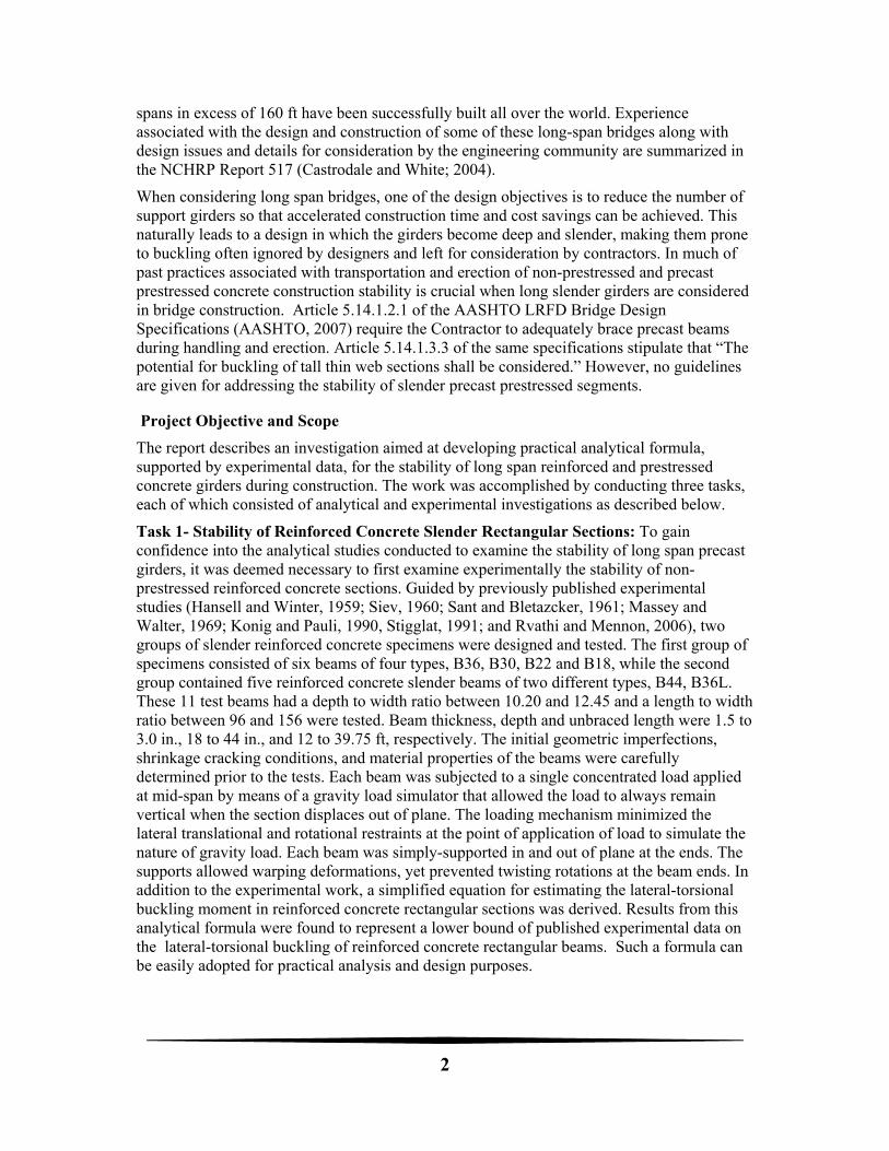
spans in excess of 160 ft have been successfully built all over the world. Experience associated with the design and construction of some of these long-span bridges along with design issues and details for consideration by the engineering community are summarized in the NCHRP Report 517 (Castrodale and White; 2004).

When considering long span bridges, one of the design objectives is to reduce the number of support girders so that accelerated construction time and cost savings can be achieved. This naturally leads to a design in which the girders become deep and slender, making them prone to buckling often ignored by designers and left for consideration by contractors. In much of past practices associated with transportation and erection of non-prestressed and precast prestressed concrete construction stability is crucial when long slender girders are considered in bridge construction. Article 5.14.1.2.1 of the AASHTO LRFD Bridge Design Specifications (AASHTO, 2007) require the Contractor to adequately brace precast beams during handling and erection. Article 5.14.1.3.3 of the same specifications stipulate that “The potential for buckling of tall thin web sections shall be considered.” However, no guidelines are given for addressing the stability of slender precast prestressed segments.

Project Objective and Scope

The report describes an investigation aimed at developing practical analytical formula, supported by experimental data, for the stability of long span reinforced and prestressed concrete girders during construction. The work was accomplished by conducting three tasks, each of which consisted of analytical and experimental investigations as described below.

Task 1- Stability of Reinforced Concrete Slender Rectangular Sections: To gain confidence into the analytical studies conducted to examine the stability of long span precast girders, it was deemed necessary to first examine experimentally the stability of non-prestressed reinforced concrete sections. Guided by previously published experimental studies (Hansell and Winter, 1959; Siev, 1960; Sant and Bletazcker, 1961; Massey and Walter, 1969; Konig and Pauli, 1990, Stigglat, 1991; and Rvathi and Mennon, 2006), two groups of slender reinforced concrete specimens were designed and tested. The first group of specimens consisted of six beams of four types, B36, B30, B22 and B18, while the second group contained five reinforced concrete slender beams of two different types, B44, B36L. These 11 test beams had a depth to width ratio between 10.20 and 12.45 and a length to width ratio between 96 and 156 were tested. Beam thickness, depth and unbraced length were 1.5 to 3.0 in., 18 to 44 in., and 12 to 39.75 ft, respectively. The initial geometric imperfections, shrinkage cracking conditions, and material properties of the beams were carefully determined prior to the tests. Each beam was subjected to a single concentrated load applied at mid-span by means of a gravity load simulator that allowed the load to always remain vertical when the section displaces out of plane. The loading mechanism minimized the lateral translational and rotational restraints at the point of application of load to simulate the nature of gravity load. Each beam was simply-supported in and out of plane at the ends. The supports allowed warping deformations, yet prevented twisting rotations at the beam ends. In addition to the experimental work, a simplified equation for estimating the lateral-torsional buckling moment in reinforced concrete rectangular sections was derived. Results from this analytical formula were found to represent a lower bound of published experimental data on the lateral-torsional buckling of reinforced concrete rectangular beams. Such a formula can be easily adopted for practical analysis and design purposes.

3

Task 2- Stability of Prestressed Concrete Slender Rectangular Sections: Rectangular prestressed sections were investigated to determine if and how the prestressing force affected the lateral buckling stability of girders having thin rectangular sections. Several authors such as Magnel (1950), Billig (1953), and Leonhardt (1955) had come to the conclusion a prestressed concrete beam where the strands were bonded to the concrete cannot buckle. Magnel’s (1950) early tests verified his theory. Later experimental and analytical work by Stratford (1999) and Muller (1962) agreed with the earlier findings that prestressing with bonded reinforcement should not influence the buckling load of concrete members; yet, unbonded posttensioning would affect the buckling resistance. Tests of six prestensioned girders with length-to-width ratios of 120 and depth-to-width ratios from 7.5 to 11 were tested. The average prestressing force varied from 450 psi to 900 psi. The prestressed beams were loaded identically to the non-prestressed beams. The experimental buckling loads were compared with theoretical predictions. Of particular concern was the influence of initial sweep on the lateral stability of the girders; for all experiments, initial sweep and sweep deformations were measured. Theoretical equations were modified for prestressed and non-prestressed beams to account for sweep.

Task 3- Thermal Behavior of a BT-54 Prestresssed Concrete Girders: A potential cause of lateral instability of long-span bridge girders is the lateral sweep which occurs. Some engineers considered that unsymmetric heating of the girders due to solar radiation was a cause of large sweep deformations which caused excessive lateral sway leading to instability. A 100-ft long BT-54 was constructed with internal and external instrumentation to measure such thermal sweep. Data were recorded for over a year. A maximum sweep of 0.5 inch was recorded due to solar heating. Further, a 5-ft long section was constructed and instrumented to accurately study the heat transfer through a BT-54 section so that realistic analytical estimates could be made for any shape bridge girder. Two principal findings follow:

(1) The maximum temperature difference over the cross section of the girder occurred at approximately 2 pm. The maximum vertical temperature difference was 30 degrees F in the summer and the minimum temperature difference was 7 degrees F in the winter. The lateral temperature differences were in the range of 23 to 29 degrees F for all four seasons.

(2) The nonlinear analysis of the girder subjected to temperature and self-weight loading determined that the maximum vertical displacement was 0.68 inches in the summer and 0.25 inches in the winter. The lateral displacement of the 100 ft long girder was determined to be 0.47 to 0.55 inches. The nonlinear analysis did not determine any stability problems of the girder associated with thermal effects.

Findings and Recommendations

Results of Task 1 analytical and experimental investigation showed that the lateral torsional buckling moment, crM ,of a slender reinforced concrete beam having a rectangular section can be computed from the following equation:

4

L

IEC

L

dbECM yc

bc

bcr

2.1

10

3

  (1.1)

where

cE = modulus of elasticity of concrete

d = effective section depth

b = section width

L = unbraced length of the beam

yI = moment of inertia about the beam minor axis

Cb = moment modification factor for nonuniform moment diagrams when both ends of the unsupported segments are braced. Cb can conservatively be taken as unity, or calculated from (AISC, 2005):

.33435.2

5.12

max

max

CBA

b MMMM

MC   (1.2)  

and Mmax = absolute value of maximum moment in the unbraced segment MA = absolute value of moment at quarter point of the unbraced segment MB = absolute value of moment at the centerline of the unbraced segment MC = absolute value of moment at three-quarter point of the unbraced segment

Guided by seminal work of the results of Michell (1899) and Prandtl (1900) during the last part of the 19th century and reinforced by Task 1 results, the treatment of a long-span non-prestressed and prestressed concrete girders is dealt with by considering the following lateral-torsional buckling moment of a simply supported beam subjected to flexure:

cr

BCM k

L (1.3)

where

crM : critical moment that causes lateral instability

k : coefficient that depends upon the loading and the boundary conditions

B : flexural rigidity with respect to the axis of buckling

C : torsional rigidity of the girder

Lateral stability is one of the most important problems encountered during transportation and construction of long-span girders. Such a problem was first recognized by Lebelle (1959) who investigated, analytically, the elastic stability of monosymmetric I-shaped sections and presented solutions, most of which had already been treated by Pradtl (1899), Timoshenko (1913), and Marshall (1948). For a simply supported girder subjected to a uniformly

5

distributed load applied the centroid of the girder and rotationally restrained at both ends, Eq. (1.3) can be expressed in the form:

328.4

y

cr

EI GJq

L (1.4)

where

crq : critical uniform load above which lateral-torsional buckling occurs.

E : modulus of elasticity

G : shear modulus

yI : moment of inertia about the principal minor axis of the section.

J : St. Venant’s torsion coefficient for the girder section

Lebelle (1959) also addressed the stability of a long girder suspended by cable lifting loops at the girder ends above the girder center of gravity. Lebelle’s solutions were further discussed by Muller (1962) who presented Lebelle’s work in a practical form suitable for design purposes. For the case in the which the girder is simply supported and subjected to a uniformly distributed load, the following formula can be used to compute the critical load at which lateral instability of the girder occurs:

1 2328.4

fy

cr

EI GJq k k

L (1.5)

Where

01

(2 )1 0.72

fyEIy

kL GJ

(1.6)

220

2 2

21

4

fyEI h

kGJ L

(1.7)

1 2

21 1

fy

f fy y

I

I I

(1.8)

in which

0y = distance of the point of load application to the shear center. It is negative if the load is

applied below the shear center and positive otherwise.

0h = distance between the centroids of top and bottom flanges 1f

yI = Moment of inertia about the axis of buckling of the top flange.

2fyI = Moment of inertia about the axis of buckling of the bottom flange.

6

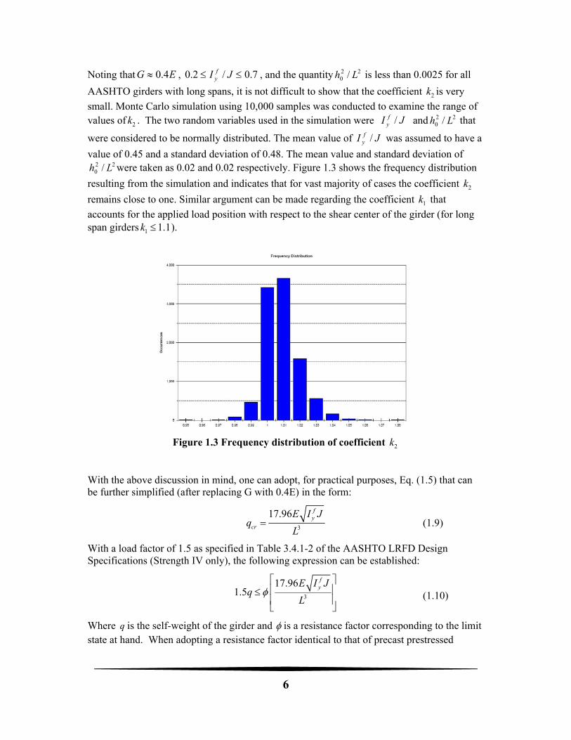
Noting that EG 4.0 , 7.0/2.0 JI fy , and the quantity 22

0 / Lh is less than 0.0025 for all

AASHTO girders with long spans, it is not difficult to show that the coefficient 2k is very

small. Monte Carlo simulation using 10,000 samples was conducted to examine the range of values of 2k . The two random variables used in the simulation were JI f

y / and 220 / Lh that

were considered to be normally distributed. The mean value of JI fy / was assumed to have a

value of 0.45 and a standard deviation of 0.48. The mean value and standard deviation of 22

0 / Lh were taken as 0.02 and 0.02 respectively. Figure 1.3 shows the frequency distribution

resulting from the simulation and indicates that for vast majority of cases the coefficient 2k

remains close to one. Similar argument can be made regarding the coefficient 1k that

accounts for the applied load position with respect to the shear center of the girder (for long span girders 1 1.1k ).

Figure 1.3 Frequency distribution of coefficient 2k

With the above discussion in mind, one can adopt, for practical purposes, Eq. (1.5) that can be further simplified (after replacing G with 0.4E) in the form:

3

17.96 fy

cr

E I Jq

L (1.9)

With a load factor of 1.5 as specified in Table 3.4.1-2 of the AASHTO LRFD Design Specifications (Strength IV only), the following expression can be established:

3

17.961.5

fyE I J

qL

(1.10)

Where q is the self-weight of the girder and is a resistance factor corresponding to the limit state at hand. When adopting a resistance factor identical to that of precast prestressed

7

girders under flexure ( 1 ), and statistical parameters similar to those used for the calibration of LRFD Bridge Design Code (Nowak, 1999), it was found that the ensuing reliability index was 2.67, which is lower than the target reliability index of 3.5 adopted in AASHTO LRFD Design Specifications (2007). To bring the reliability index to a level comparable to that of AAHTO LRFD Design specifications ( 3.5 ), Monte Carlo simulation was performed. The result of the simulation indicated that a value of 0.78 will result in a reliability index of 3.52 which is sufficient for the problem at hand. From a practical point of view a value of 0.75 is adopted hereafter, which results in a reliability index of 3.77. By doing so, we can write:

3

17.961.5 0.75

fyE I J

qL

(1.11)

From which the maximum girder length can be computed from the following suggested equation:

1 3

2fyE I J

Lq

(1.12)

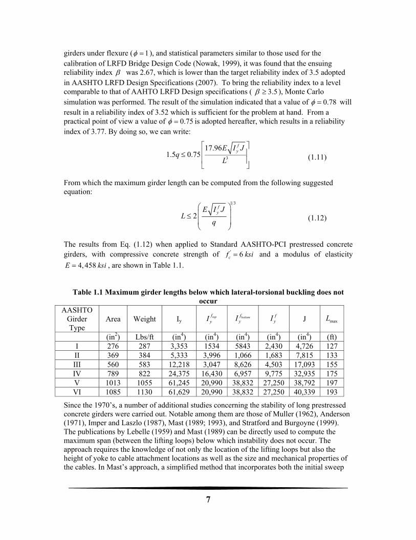
The results from Eq. (1.12) when applied to Standard AASHTO-PCI prestressed concrete girders, with compressive concrete strength of ' 6cf ksi and a modulus of elasticity

4, 458E ksi , are shown in Table 1.1.

Table 1.1 Maximum girder lengths below which lateral-torsional buckling does not occur

AASHTO Girder Type

Area Weight Iy topf

yI bottomfyI f

yI J maxL

(in2) Lbs/ft (in4) (in4) (in4) (in4) (in4) (ft) I 276 287 3,353 1534 5843 2,430 4,726 127 II 369 384 5,333 3,996 1,066 1,683 7,815 133 III 560 583 12,218 3,047 8,626 4,503 17,093 155 IV 789 822 24,375 16,430 6,957 9,775 32,935 175 V 1013 1055 61,245 20,990 38,832 27,250 38,792 197 VI 1085 1130 61,629 20,990 38,832 27,250 40,339 193

Since the 1970’s, a number of additional studies concerning the stability of long prestressed concrete girders were carried out. Notable among them are those of Muller (1962), Anderson (1971), Imper and Laszlo (1987), Mast (1989; 1993), and Stratford and Burgoyne (1999). The publications by Lebelle (1959) and Mast (1989) can be directly used to compute the maximum span (between the lifting loops) below which instability does not occur. The approach requires the knowledge of not only the location of the lifting loops but also the height of yoke to cable attachment locations as well as the size and mechanical properties of the cables. In Mast’s approach, a simplified method that incorporates both the initial sweep

8

and the lifting loop placement locations. Mast (1993) presented an approach to address the stability of long prestressed girders resting on flexible supports, a case addressing the stability of such girders in transit. PCI Design Handbook adopts the approach presented by Mast (1989, 1993) but remains silent on the stability of long girders when they are erected.

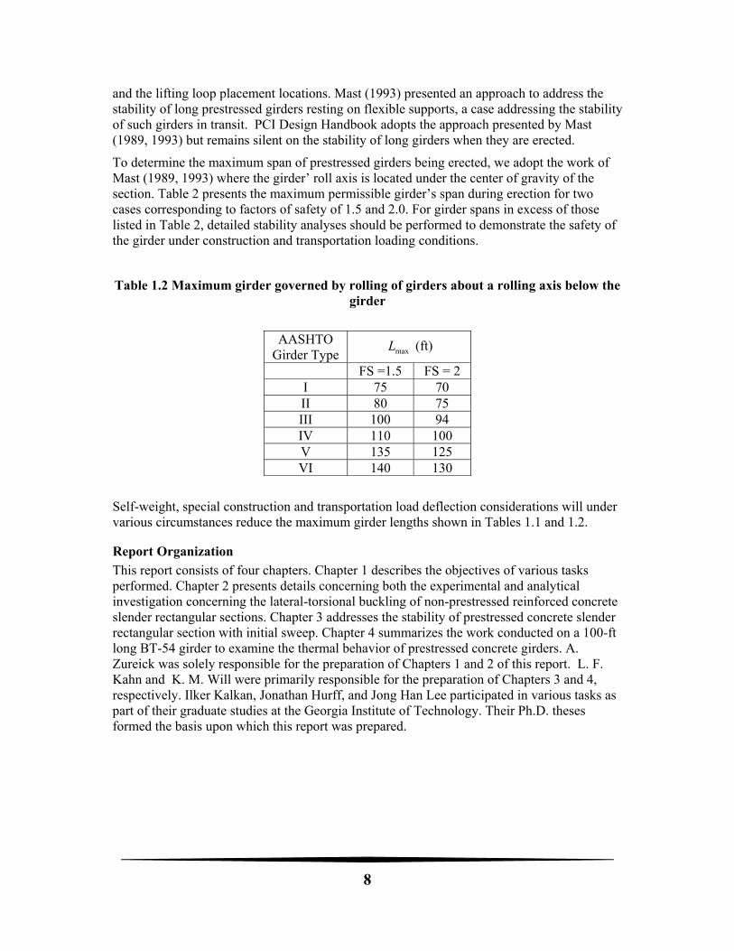
To determine the maximum span of prestressed girders being erected, we adopt the work of Mast (1989, 1993) where the girder’ roll axis is located under the center of gravity of the section. Table 2 presents the maximum permissible girder’s span during erection for two cases corresponding to factors of safety of 1.5 and 2.0. For girder spans in excess of those listed in Table 2, detailed stability analyses should be performed to demonstrate the safety of the girder under construction and transportation loading conditions.

Table 1.2 Maximum girder governed by rolling of girders about a rolling axis below the girder

AASHTO

Girder Type maxL (ft)

FS =1.5 FS = 2 I 75 70 II 80 75 III 100 94 IV 110 100 V 135 125 VI 140 130

Self-weight, special construction and transportation load deflection considerations will under various circumstances reduce the maximum girder lengths shown in Tables 1.1 and 1.2.

Report Organization

This report consists of four chapters. Chapter 1 describes the objectives of various tasks performed. Chapter 2 presents details concerning both the experimental and analytical investigation concerning the lateral-torsional buckling of non-prestressed reinforced concrete slender rectangular sections. Chapter 3 addresses the stability of prestressed concrete slender rectangular section with initial sweep. Chapter 4 summarizes the work conducted on a 100-ft long BT-54 girder to examine the thermal behavior of prestressed concrete girders. A. Zureick was solely responsible for the preparation of Chapters 1 and 2 of this report. L. F. Kahn and K. M. Will were primarily responsible for the preparation of Chapters 3 and 4, respectively. Ilker Kalkan, Jonathan Hurff, and Jong Han Lee participated in various tasks as part of their graduate studies at the Georgia Institute of Technology. Their Ph.D. theses formed the basis upon which this report was prepared.

9

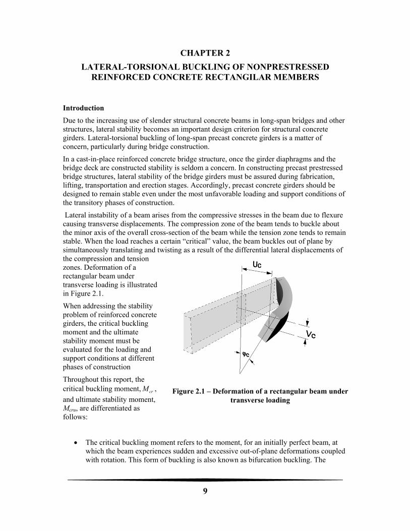
Figure 2.1 – Deformation of a rectangular beam under transverse loading

CHAPTER 2

LATERAL-TORSIONAL BUCKLING OF NONPRESTRESSED REINFORCED CONCRETE RECTANGILAR MEMBERS

Introduction

Due to the increasing use of slender structural concrete beams in long-span bridges and other structures, lateral stability becomes an important design criterion for structural concrete girders. Lateral-torsional buckling of long-span precast concrete girders is a matter of concern, particularly during bridge construction.

In a cast-in-place reinforced concrete bridge structure, once the girder diaphragms and the bridge deck are constructed stability is seldom a concern. In constructing precast prestressed bridge structures, lateral stability of the bridge girders must be assured during fabrication, lifting, transportation and erection stages. Accordingly, precast concrete girders should be designed to remain stable even under the most unfavorable loading and support conditions of the transitory phases of construction.

Lateral instability of a beam arises from the compressive stresses in the beam due to flexure causing transverse displacements. The compression zone of the beam tends to buckle about the minor axis of the overall cross-section of the beam while the tension zone tends to remain stable. When the load reaches a certain “critical” value, the beam buckles out of plane by simultaneously translating and twisting as a result of the differential lateral displacements of the compression and tension zones. Deformation of a rectangular beam under transverse loading is illustrated in Figure 2.1.

When addressing the stability problem of reinforced concrete girders, the critical buckling moment and the ultimate stability moment must be evaluated for the loading and support conditions at different phases of construction

Throughout this report, the critical buckling moment, crM ,

and ultimate stability moment, Mcru, are differentiated as follows:

The critical buckling moment refers to the moment, for an initially perfect beam, at which the beam experiences sudden and excessive out-of-plane deformations coupled with rotation. This form of buckling is also known as bifurcation buckling. The

10

ultimate stability moment occurs in a beam with initial geometric imperfections, and therefore it undergoes deformations and rotation throughout the entire stage of loading.

The ultimate stability moment denotes the greatest moment carried by an initially imperfect beam, beyond which excessive lateral displacements and rotations are experienced.

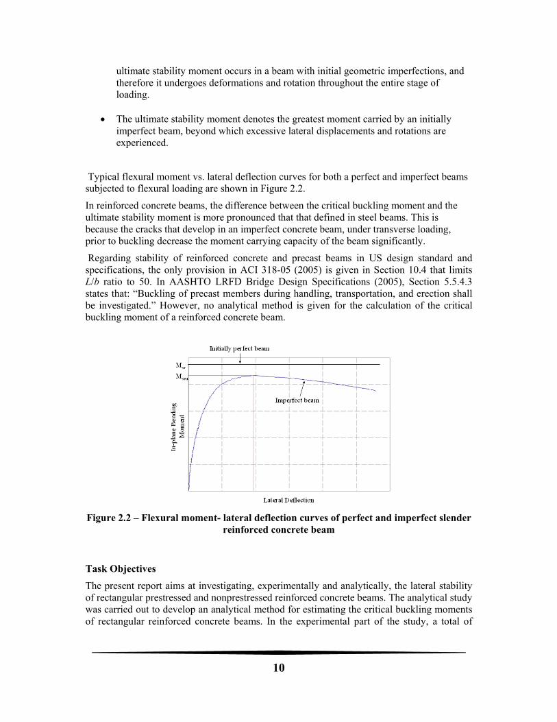
Typical flexural moment vs. lateral deflection curves for both a perfect and imperfect beams subjected to flexural loading are shown in Figure 2.2.

In reinforced concrete beams, the difference between the critical buckling moment and the ultimate stability moment is more pronounced that that defined in steel beams. This is because the cracks that develop in an imperfect concrete beam, under transverse loading, prior to buckling decrease the moment carrying capacity of the beam significantly.

Regarding stability of reinforced concrete and precast beams in US design standard and specifications, the only provision in ACI 318-05 (2005) is given in Section 10.4 that limits L/b ratio to 50. In AASHTO LRFD Bridge Design Specifications (2005), Section 5.5.4.3 states that: “Buckling of precast members during handling, transportation, and erection shall be investigated.” However, no analytical method is given for the calculation of the critical buckling moment of a reinforced concrete beam.

Figure 2.2 – Flexural moment- lateral deflection curves of perfect and imperfect slender reinforced concrete beam

Task Objectives

The present report aims at investigating, experimentally and analytically, the lateral stability of rectangular prestressed and nonprestressed reinforced concrete beams. The analytical study was carried out to develop an analytical method for estimating the critical buckling moments of rectangular reinforced concrete beams. In the experimental part of the study, a total of

11

eleven slender rectangular reinforced concrete beams were tested to validate the analytical methods proposed for examining the lateral-torsional buckling of reinforced concrete beams. Attention is given to the effects of the initial geometric imperfections and shrinkage on the lateral stability of reinforced concrete beams.

Previous Studies

Over the past six decades, several experimental and analytical investigations aimed at addressing the lateral stability of reinforced concrete beams have been carried out. Highlights of studies pertaining to reinforced concrete rectangular sections are, hereafter, presented.

Marshall (1948): This was the first study that resulted in the development of critical load expressions for a laterally-unsupported beam under for:

A concentrated load at midspan

2

16.93cr B

LP GC (2.1)

A uniformly distributed load throughout the span;

GCBL

qcr 3

6.28 (2.2)

Equal and opposite bending moments at the beam ends:

GCBL

M cr

47.8 (2.3)

In the above equations, Pcr , crq , and Mcr are the critical concentrated load, critical uniformly

distributed load, and the critical end moments , respectively. L is the unbraced length of the beam; B and C are the out-of-plane flexural and the torsional rigidities of the beam, respectively. For the case of uniformly distributed load, Marshall (1948) proposed that B and C be taken as

12500,2

3dbB (2.4)

3900

3dbC (2.5)

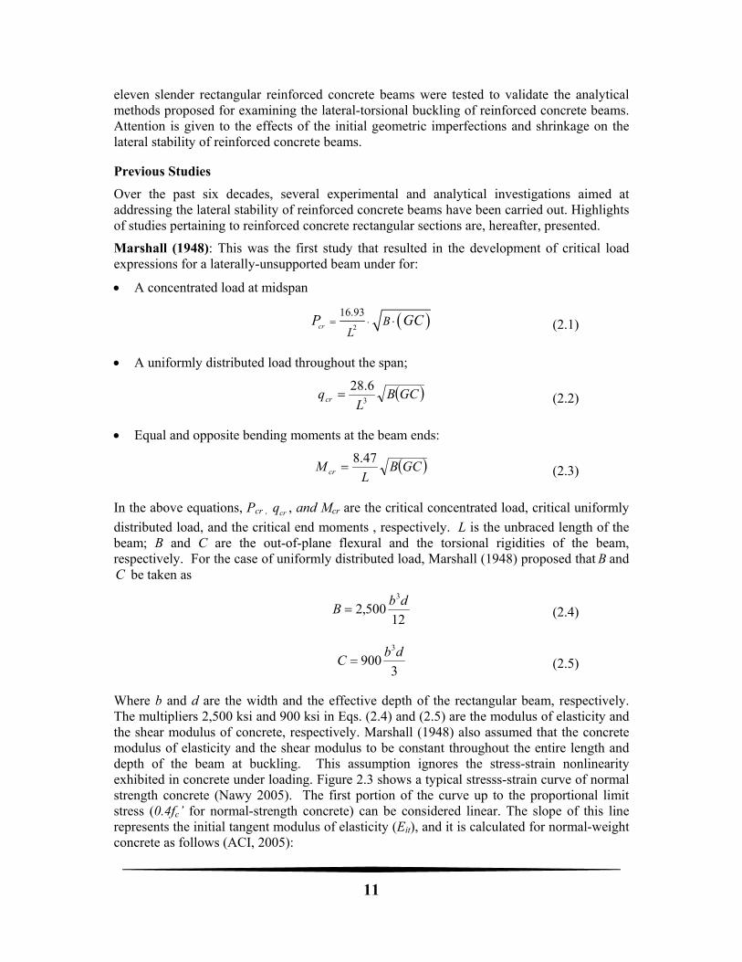
Where b and d are the width and the effective depth of the rectangular beam, respectively. The multipliers 2,500 ksi and 900 ksi in Eqs. (2.4) and (2.5) are the modulus of elasticity and the shear modulus of concrete, respectively. Marshall (1948) also assumed that the concrete modulus of elasticity and the shear modulus to be constant throughout the entire length and depth of the beam at buckling. This assumption ignores the stress-strain nonlinearity exhibited in concrete under loading. Figure 2.3 shows a typical stresss-strain curve of normal strength concrete (Nawy 2005). The first portion of the curve up to the proportional limit stress (0.4fc’ for normal-strength concrete) can be considered linear. The slope of this line represents the initial tangent modulus of elasticity (Eit), and it is calculated for normal-weight concrete as follows (ACI, 2005):

12

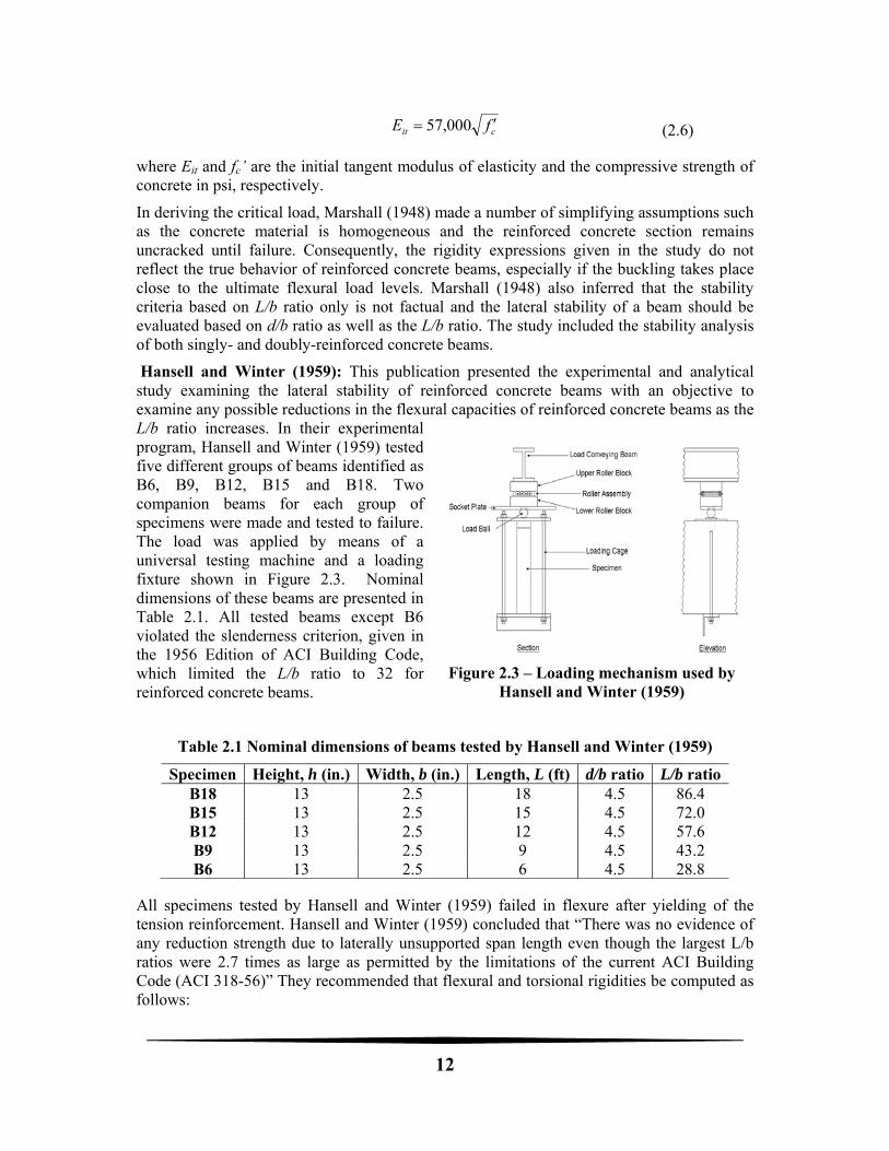
Figure 2.3 – Loading mechanism used by Hansell and Winter (1959)

cit fE 000,57 (2.6)

where Eit and fc’ are the initial tangent modulus of elasticity and the compressive strength of concrete in psi, respectively.

In deriving the critical load, Marshall (1948) made a number of simplifying assumptions such as the concrete material is homogeneous and the reinforced concrete section remains uncracked until failure. Consequently, the rigidity expressions given in the study do not reflect the true behavior of reinforced concrete beams, especially if the buckling takes place close to the ultimate flexural load levels. Marshall (1948) also inferred that the stability criteria based on L/b ratio only is not factual and the lateral stability of a beam should be evaluated based on d/b ratio as well as the L/b ratio. The study included the stability analysis of both singly- and doubly-reinforced concrete beams.

Hansell and Winter (1959): This publication presented the experimental and analytical study examining the lateral stability of reinforced concrete beams with an objective to examine any possible reductions in the flexural capacities of reinforced concrete beams as the L/b ratio increases. In their experimental program, Hansell and Winter (1959) tested five different groups of beams identified as B6, B9, B12, B15 and B18. Two companion beams for each group of specimens were made and tested to failure. The load was applied by means of a universal testing machine and a loading fixture shown in Figure 2.3. Nominal dimensions of these beams are presented in Table 2.1. All tested beams except B6 violated the slenderness criterion, given in the 1956 Edition of ACI Building Code, which limited the L/b ratio to 32 for reinforced concrete beams.

Table 2.1 Nominal dimensions of beams tested by Hansell and Winter (1959)

Specimen Height, h (in.) Width, b (in.) Length, L (ft) d/b ratio L/b ratioB18 13 2.5 18 4.5 86.4 B15 13 2.5 15 4.5 72.0 B12 13 2.5 12 4.5 57.6 B9 13 2.5 9 4.5 43.2 B6 13 2.5 6 4.5 28.8

All specimens tested by Hansell and Winter (1959) failed in flexure after yielding of the tension reinforcement. Hansell and Winter (1959) concluded that “There was no evidence of any reduction strength due to laterally unsupported span length even though the largest L/b ratios were 2.7 times as large as permitted by the limitations of the current ACI Building Code (ACI 318-56)” They recommended that flexural and torsional rigidities be computed as follows:

13

3

sec12

b cB E

  (2.7)

23sec 1 0.35

2 1 3

E b c bC

d

  (2.8)

where c is the depth of the neutral axis from the top beam surface, b is the beam width, d is the effective depth to the centroid of reinforcement, Esec is the secant modulus of elasticity corresponding to the extreme compression fiber strain at buckling, and is Poisson’s ratio.

Siev (1960): In this work analytical and experimental investigations concerning the lateral buckling of slender reinforced concrete beams were carried out. It was recommended that critical moment be computed from:

1

2

cr B CC L

CM

(2.9)

where C1 and C2 are the constants corresponding to the loading and support conditions of the beam, respectively. The flexural rigidity B was proposed for the three different states as applicable:

For the uncracked state:

3

12u c

b hEB

(2.10)

For the cracked elastic state:

22

6 4

c oc

c

c bb

a c d c

EMB

(2.11)

where M is the in-plane bending moment; σc is the extreme compression fiber stress corresponding to M; bo is the horizontal distance between the centroids of the reinforcing bars, a is the internal moment arm of the section, and c is the depth to the neutral axis. As a result of assuming a triangular stress distribution in the compression zone of the section,

3cda .

For the plastic state:

2

212

p ep

ecp

c c

cc

b M

aB

(2.12)

where cp and ce are the depths of the plastic and elastic portions of the compression zone, respectively, c is the strain at the extreme compression fibers.

The torsional rigidity is expressed as follows:

14

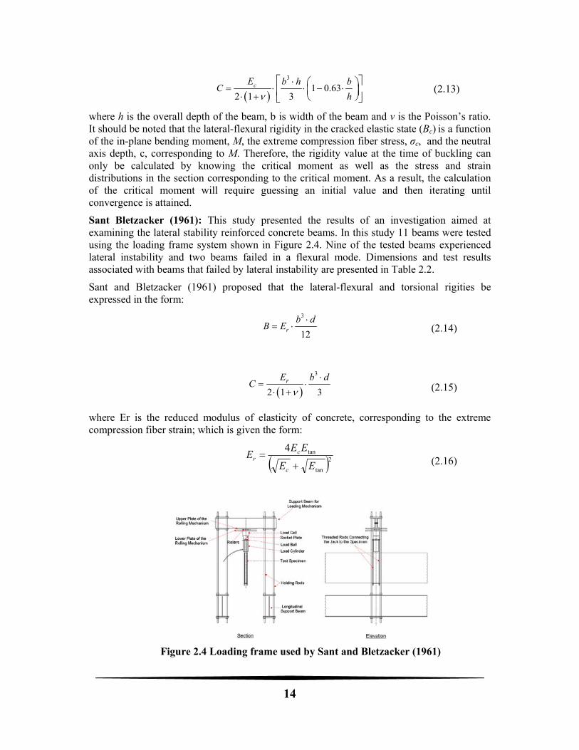
Figure 2.4 Loading frame used by Sant and Bletzacker (1961)

3

1 0.632 1 3

cE b h bC

h

(2.13)

where h is the overall depth of the beam, b is width of the beam and ν is the Poisson’s ratio. It should be noted that the lateral-flexural rigidity in the cracked elastic state (Bc) is a function of the in-plane bending moment, M, the extreme compression fiber stress, σc, and the neutral axis depth, c, corresponding to M. Therefore, the rigidity value at the time of buckling can only be calculated by knowing the critical moment as well as the stress and strain distributions in the section corresponding to the critical moment. As a result, the calculation of the critical moment will require guessing an initial value and then iterating until convergence is attained.

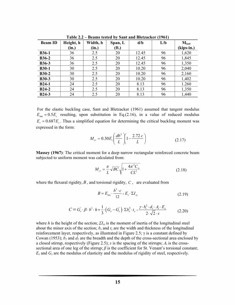
Sant Bletzacker (1961): This study presented the results of an investigation aimed at examining the lateral stability reinforced concrete beams. In this study 11 beams were tested using the loading frame system shown in Figure 2.4. Nine of the tested beams experienced lateral instability and two beams failed in a flexural mode. Dimensions and test results associated with beams that failed by lateral instability are presented in Table 2.2.

Sant and Bletzacker (1961) proposed that the lateral-flexural and torsional rigities be expressed in the form:

3

12r

b dB E

(2.14)

3

2 1 3rE b d

C

(2.15)

where Er is the reduced modulus of elasticity of concrete, corresponding to the extreme compression fiber strain; which is given the form:

2tan

tan4

EE

EEE

c

cr

(2.16)

15

Table 2.2 – Beams tested by Sant and Bletzacker (1961) Beam ID Height, h

(in.) Width, b

(in.) Span, L

(ft.) d/b L/b Mtest

(kips-in.) B36-1 36 2.5 20 12.45 96 1,620 B36-2 36 2.5 20 12.45 96 1,845 B36-3 36 2.5 20 12.45 96 1,350 B30-1 30 2.5 20 10.20 96 2,040 B30-2 30 2.5 20 10.20 96 2,160 B30-3 30 2.5 20 10.20 96 1,402 B24-1 24 2.5 20 8.13 96 1.260 B24-2 24 2.5 20 8.13 96 1,350 B24-3 24 2.5 20 8.13 96 1,440

For the elastic buckling case, Sant and Bletzacker (1961) assumed that tangent modulus

cEE 5.0tan resulting, upon substitution in Eq.(2.16), in a value of reduced modulus

cr EE 687.0 . Thus a simplified equation for determining the critical buckling moment was

expressed in the form:

L

c

L

dbEM ccr

72.2130.0

3

(2.17)

Massey (1967): The critical moment for a deep narrow rectangular reinforced concrete beam subjected to uniform moment was calculated from:

2

241

CL

CBC

LM w

cr

  (2.18)

where the flexural rigidity, B , and torsional rigidity, C , are evaluated from

3

sec12

s sy

b cB E E I

  (2.19)

2

3 1 1' ' 31

3 2 2t s

c s c s sb d A E

G b h G G b ts

C

  (2.20)

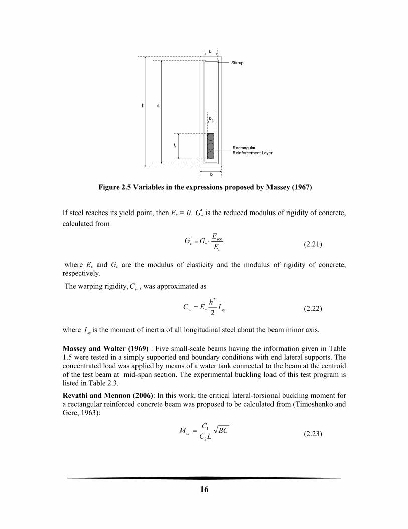
where h is the height of the section; ΣIsy is the moment of inertia of the longitudinal steel about the minor axis of the section; bs and ts are the width and thickness of the longitudinal reinforcement layer, respectively, as illustrated in Figure 2.5; γ is a constant defined by Cowan (1953); b1 and d1 are the breadth and the depth of the cross-sectional area enclosed by a closed stirrup, respectively (Figure 2.5); s is the spacing of the stirrups; At is the cross-sectional area of one leg of the stirrup; β is the coefficient for St. Venant’s torsional constant; Es and Gs are the modulus of elasticity and the modulus of rigidity of steel, respectively.

16

Figure 2.5 Variables in the expressions proposed by Massey (1967)

If steel reaches its yield point, then Es = 0. cG is the reduced modulus of rigidity of concrete,

calculated from

sec'

cc

cE

GE

G   (2.21)

where Ec and Gc are the modulus of elasticity and the modulus of rigidity of concrete, respectively.

The warping rigidity, wC , was approximated as

sycw Ih

EC2

2

  (2.22)

where syI is the moment of inertia of all longitudinal steel about the beam minor axis.

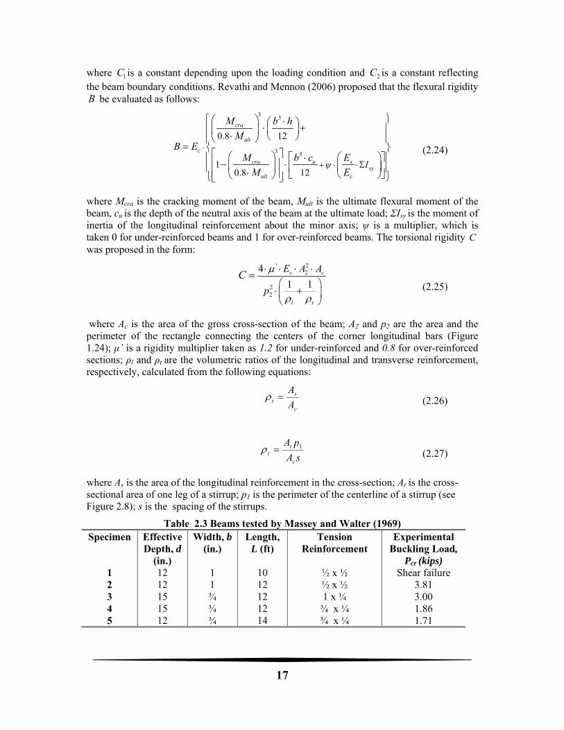
Massey and Walter (1969) : Five small-scale beams having the information given in Table 1.5 were tested in a simply supported end boundary conditions with end lateral supports. The concentrated load was applied by means of a water tank connected to the beam at the centroid of the test beam at mid-span section. The experimental buckling load of this test program is listed in Table 2.3.

Revathi and Mennon (2006): In this work, the critical lateral-torsional buckling moment for a rectangular reinforced concrete beam was proposed to be calculated from (Timoshenko and Gere, 1963):

BCLC

CM cr

2

1   (2.23)

17

where 1C is a constant depending upon the loading condition and 2C is a constant reflecting the beam boundary conditions. Revathi and Mennon (2006) proposed that the flexural rigidity B be evaluated as follows:

3 3

3 3

0.8 12

10.8 12

cra

ult

c

cra u ssy

ult c

I

M b h

MB E

M b c E

M E

  (2.24)

where Mcra is the cracking moment of the beam, Mult is the ultimate flexural moment of the beam, cu is the depth of the neutral axis of the beam at the ultimate load; ΣIsy is the moment of inertia of the longitudinal reinforcement about the minor axis; ψ is a multiplier, which is taken 0 for under-reinforced beams and 1 for over-reinforced beams. The torsional rigidity C was proposed in the form:

' 22

22

4

1 1s c

l t

E A A

p

C

 (2.25)

where Ac is the area of the gross cross-section of the beam; A2 and p2 are the area and the perimeter of the rectangle connecting the centers of the corner longitudinal bars (Figure 1.24); μ’ is a rigidity multiplier taken as 1.2 for under-reinforced and 0.8 for over-reinforced sections; ρl and ρt are the volumetric ratios of the longitudinal and transverse reinforcement, respectively, calculated from the following equations:

c

si A

A   (2.26)

sA

pA

c

tt

1   (2.27)

where As is the area of the longitudinal reinforcement in the cross-section; At is the cross-sectional area of one leg of a stirrup; p1 is the perimeter of the centerline of a stirrup (see Figure 2.8); s is the spacing of the stirrups.

Table 2.3 Beams tested by Massey and Walter (1969) Specimen Effective

Depth, d (in.)

Width, b (in.)

Length, L (ft)

Tension Reinforcement

Experimental Buckling Load,

Pcr (kips) 1 12 1 10 ½ x ½ Shear failure 2 12 1 12 ½ x ½ 3.81 3 15 ¾ 12 1 x ¼ 3.00 4 15 ¾ 12 ¾ x ¼ 1.86 5 12 ¾ 14 ¾ x ¼ 1.71

18

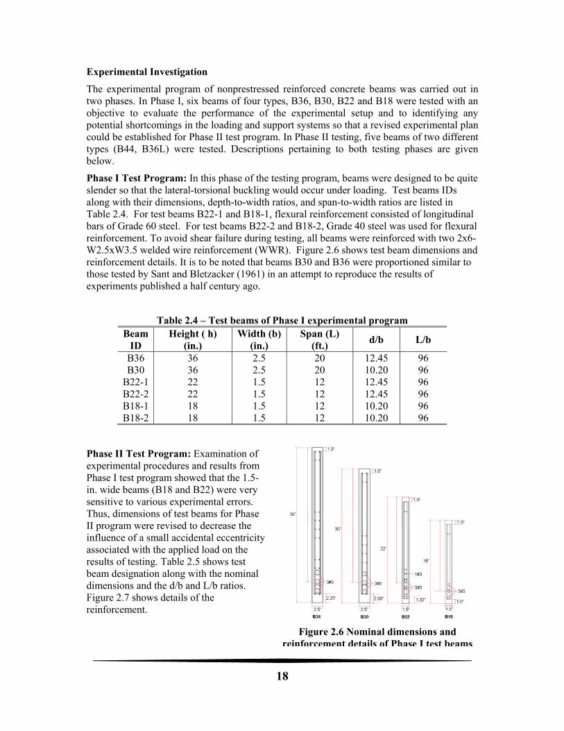
Figure 2.6 Nominal dimensions and reinforcement details of Phase I test beams

Experimental Investigation

The experimental program of nonprestressed reinforced concrete beams was carried out in two phases. In Phase I, six beams of four types, B36, B30, B22 and B18 were tested with an objective to evaluate the performance of the experimental setup and to identifying any potential shortcomings in the loading and support systems so that a revised experimental plan could be established for Phase II test program. In Phase II testing, five beams of two different types (B44, B36L) were tested. Descriptions pertaining to both testing phases are given below.

Phase I Test Program: In this phase of the testing program, beams were designed to be quite slender so that the lateral-torsional buckling would occur under loading. Test beams IDs along with their dimensions, depth-to-width ratios, and span-to-width ratios are listed in Table 2.4. For test beams B22-1 and B18-1, flexural reinforcement consisted of longitudinal bars of Grade 60 steel. For test beams B22-2 and B18-2, Grade 40 steel was used for flexural reinforcement. To avoid shear failure during testing, all beams were reinforced with two 2x6-W2.5xW3.5 welded wire reinforcement (WWR). Figure 2.6 shows test beam dimensions and reinforcement details. It is to be noted that beams B30 and B36 were proportioned similar to those tested by Sant and Bletzacker (1961) in an attempt to reproduce the results of experiments published a half century ago.

Table 2.4 – Test beams of Phase I experimental program Beam

ID Height ( h)

(in.) Width (b)

(in.) Span (L)

(ft.) d/b L/b

B36 36 2.5 20 12.45 96 B30 36 2.5 20 10.20 96

B22-1 22 1.5 12 12.45 96 B22-2 22 1.5 12 12.45 96 B18-1 18 1.5 12 10.20 96 B18-2 18 1.5 12 10.20 96

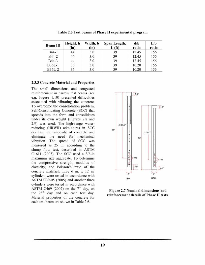
Phase II Test Program: Examination of experimental procedures and results from Phase I test program showed that the 1.5-in. wide beams (B18 and B22) were very sensitive to various experimental errors. Thus, dimensions of test beams for Phase II program were revised to decrease the influence of a small accidental eccentricity associated with the applied load on the results of testing. Table 2.5 shows test beam designation along with the nominal dimensions and the d/b and L/b ratios. Figure 2.7 shows details of the reinforcement.

19

Figure 2.7 Nominal dimensions and reinforcement details of Phase II tests

Table 2.5 Test beams of Phase II experimental program

Beam ID Height, h

(in) Width, b

(in) Span Length,

L (ft) d/b

ratio L/b

ratio B44-1 44 3.0 39 12.45 156 B44-2 44 3.0 39 12.45 156 B44-3 44 3.0 39 12.45 156

B36L-1 36 3.0 39 10.20 156 B36L-2 36 3.0 39 10.20 156

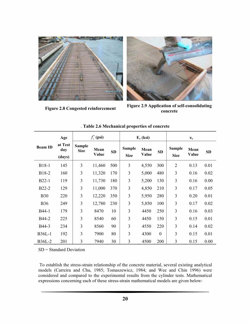
2.3.3 Concrete Material and Properties

The small dimensions and congested reinforcement in narrow test beams (see e.g. Figure 1.10) presented difficulties associated with vibrating the concrete. To overcome the consolidation problem, Self-Consolidating Concrete (SCC) that spreads into the form and consolidates under its own weight (Figures 2.8 and 2.9) was used. The high-range water-reducing (HRWR) admixtures in SCC decrease the viscosity of concrete and eliminate the need for mechanical vibration. The spread of SCC was measured as 25 in. according to the slump flow test, described in ASTM C1611 (2005). The SCC used a 3/8-in maximum size aggregate. To determine the compressive strength, modulus of elasticity, and Poisson’s ratio of the concrete material, three 6 in. x 12 in. cylinders were tested in accordance with ASTM C39-05 (2005) and another three cylinders were tested in accordance with ASTM C469 (2002) on the 7th day, on the 28th day and on each test day. Material properties of the concrete for each test beam are shown in Table 2.6.

20

Figure 2.8 Congested reinforcement Figure 2.9 Application of self-consolidating

concrete

. Table 2.6 Mechanical properties of concrete

Beam ID

Age

at Test day

(days)

cf (psi) Ec (ksi) υc

Sample Size

Mean Value

SD Sample

Size

Mean Value

SD Sample

Size

Mean Value

SD

B18-1 145 3 11,460 500 3 4,550 300 2 0.13 0.01

B18-2 160 3 11,320 170 3 5,000 480 3 0.16 0.02

B22-1 119 3 11,730 180 3 5,200 130 3 0.16 0.00

B22-2 129 3 11,000 370 3 4,850 210 3 0.17 0.05

B30 220 3 12,220 350 3 5,950 280 3 0.20 0.01

B36 249 3 12,780 230 3 5,850 100 3 0.17 0.02

B44-1 179 3 8470 10 3 4450 250 3 0.16 0.03

B44-2 225 3 8540 60 3 4450 150 3 0.15 0.01

B44-3 234 3 8560 90 3 4550 220 3 0.14 0.02

B36L-1 192 3 7900 80 3 4300 0 3 0.15 0.01

B36L-2 201 3 7940 30 3 4500 200 3 0.15 0.00

SD = Standard Deviation

To establish the stress-strain relationship of the concrete material, several existing analytical models (Carreira and Chu, 1985; Tomaszewicz, 1984; and Wee and Chin 1996) were considered and compared to the experimental results from the cylinder tests. Mathematical expressions concerning each of these stress-strain mathematical models are given below:

21

1- The Carreira and Chu (1985) model for high strength concrete was proposed in the form:

'

1

oc c

o

f f

  (2.28)

where and fc are the concrete strain and stress, respectively; εo is the strain at peak stress and f’c is the compressive strength of concrete according to the cylinder tests; β can be computed from:

'

1

1 c o cf E

  (2.29)

2- The Tomaszewicz (1984) model adopts equation (1.26) for the ascending portion of the stress strain curve and proposes that the descending part of the curve be expressed in the form:

'

1

oc c

o

kf f

  (2.30)

where k = f’c/2.90 with f’c given in ksi.

3- The Wee and Chin (1996) model also adopts equation (1.27) for the ascending portion of the stress-strain curve but models the descending portion with

2

1'

1 1

oc c

o

k

k

f f

k

  (2.31)

where k1 = (7.26/f’c)3.0 and k2 = (7.26/f’c)

1.3 with f’c given in ksi.

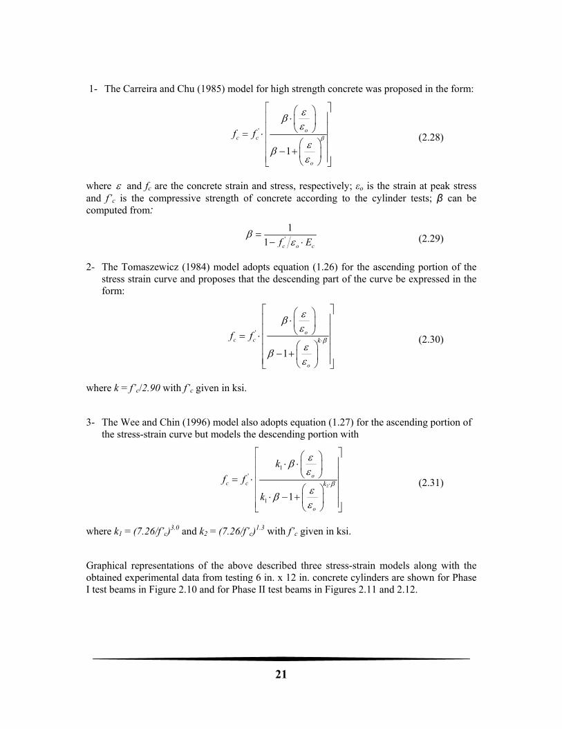
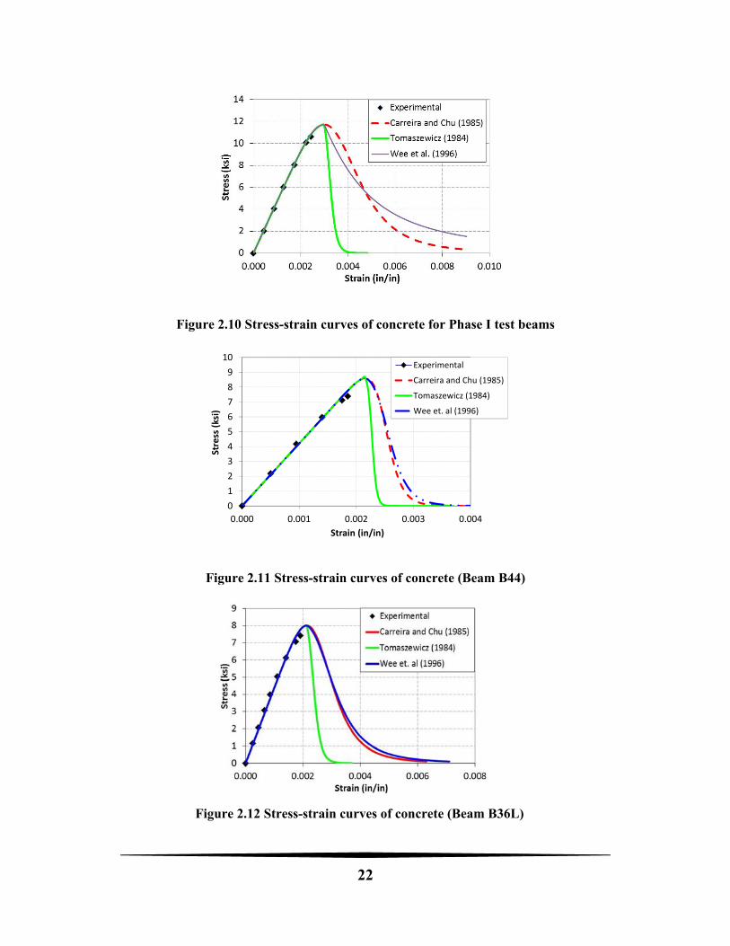
Graphical representations of the above described three stress-strain models along with the obtained experimental data from testing 6 in. x 12 in. concrete cylinders are shown for Phase I test beams in Figure 2.10 and for Phase II test beams in Figures 2.11 and 2.12.

22

Figure 2.10 Stress-strain curves of concrete for Phase I test beams

Figure 2.11 Stress-strain curves of concrete (Beam B44)

0

1

2

3

4

5

6

7

8

9

10

0.000 0.001 0.002 0.003 0.004

Stress (ksi)

Strain (in/in)

Experimental

Carreira and Chu (1985)

Tomaszewicz (1984)

Wee et. al (1996)

Figure 2.12 Stress-strain curves of concrete (Beam B36L)

23

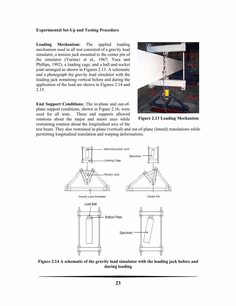
Figure 2.13 Loading Mechanism

Experimental Set-Up and Testing Procedure

Loading Mechanism: The applied loading mechanism used in all test consisted of a gravity load simulator, a tension jack mounted to the center pin of the simulator (Yarimci et al., 1967; Yura and Phillips, 1992), a loading cage, and a ball-and-socket joint arranged as shown in Figures 2.13. A schematic and a photograph the gravity load simulator with the loading jack remaining vertical before and during the application of the load are shown in Figures 2.14 and 2.15.

End Support Conditions: The in-plane and out-of-plane support conditions, shown in Figure 2.16, were used for all tests. These end supports allowed rotations about the major and minor axes while restraining rotation about the longitudinal axis of the test beam. They also restrained in-plane (vertical) and out-of-plane (lateral) translations while permitting longitudinal translation and warping deformations.

Figure 2.14 A schematic of the gravity load simulator with the loading jack before and during loading

24

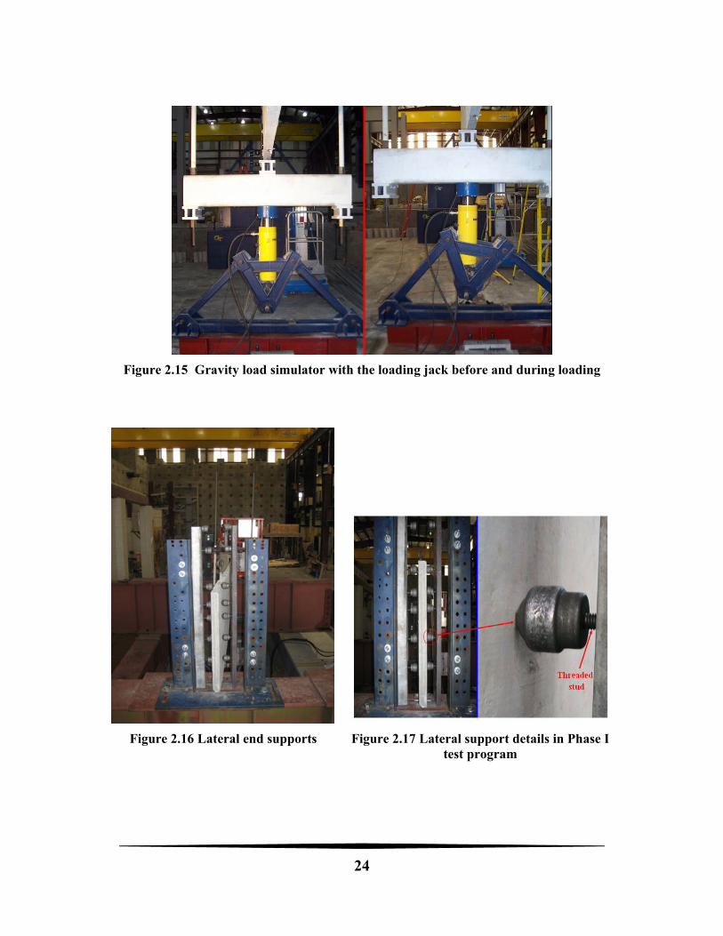
Figure 2.15 Gravity load simulator with the loading jack before and during loading

Figure 2.16 Lateral end supports

Figure 2.17 Lateral support details in Phase I test program

25

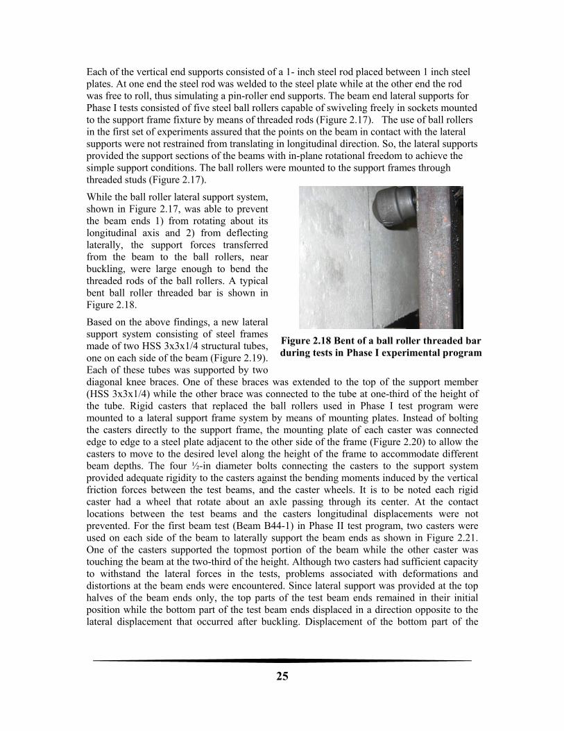
Figure 2.18 Bent of a ball roller threaded bar during tests in Phase I experimental program

Each of the vertical end supports consisted of a 1- inch steel rod placed between 1 inch steel plates. At one end the steel rod was welded to the steel plate while at the other end the rod was free to roll, thus simulating a pin-roller end supports. The beam end lateral supports for Phase I tests consisted of five steel ball rollers capable of swiveling freely in sockets mounted to the support frame fixture by means of threaded rods (Figure 2.17). The use of ball rollers in the first set of experiments assured that the points on the beam in contact with the lateral supports were not restrained from translating in longitudinal direction. So, the lateral supports provided the support sections of the beams with in-plane rotational freedom to achieve the simple support conditions. The ball rollers were mounted to the support frames through threaded studs (Figure 2.17).

While the ball roller lateral support system, shown in Figure 2.17, was able to prevent the beam ends 1) from rotating about its longitudinal axis and 2) from deflecting laterally, the support forces transferred from the beam to the ball rollers, near buckling, were large enough to bend the threaded rods of the ball rollers. A typical bent ball roller threaded bar is shown in Figure 2.18.

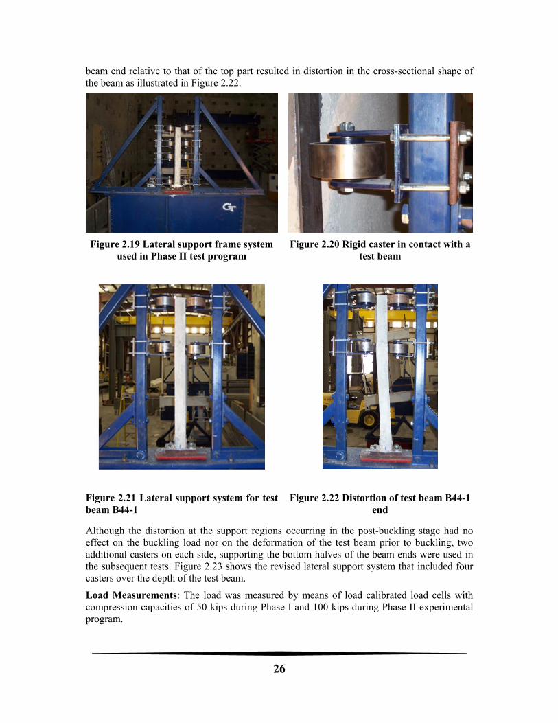
Based on the above findings, a new lateral support system consisting of steel frames made of two HSS 3x3x1/4 structural tubes, one on each side of the beam (Figure 2.19). Each of these tubes was supported by two diagonal knee braces. One of these braces was extended to the top of the support member (HSS 3x3x1/4) while the other brace was connected to the tube at one-third of the height of the tube. Rigid casters that replaced the ball rollers used in Phase I test program were mounted to a lateral support frame system by means of mounting plates. Instead of bolting the casters directly to the support frame, the mounting plate of each caster was connected edge to edge to a steel plate adjacent to the other side of the frame (Figure 2.20) to allow the casters to move to the desired level along the height of the frame to accommodate different beam depths. The four ½-in diameter bolts connecting the casters to the support system provided adequate rigidity to the casters against the bending moments induced by the vertical friction forces between the test beams, and the caster wheels. It is to be noted each rigid caster had a wheel that rotate about an axle passing through its center. At the contact locations between the test beams and the casters longitudinal displacements were not prevented. For the first beam test (Beam B44-1) in Phase II test program, two casters were used on each side of the beam to laterally support the beam ends as shown in Figure 2.21. One of the casters supported the topmost portion of the beam while the other caster was touching the beam at the two-third of the height. Although two casters had sufficient capacity to withstand the lateral forces in the tests, problems associated with deformations and distortions at the beam ends were encountered. Since lateral support was provided at the top halves of the beam ends only, the top parts of the test beam ends remained in their initial position while the bottom part of the test beam ends displaced in a direction opposite to the lateral displacement that occurred after buckling. Displacement of the bottom part of the

26

beam end relative to that of the top part resulted in distortion in the cross-sectional shape of the beam as illustrated in Figure 2.22.

Figure 2.19 Lateral support frame system used in Phase II test program

Figure 2.20 Rigid caster in contact with a test beam

Figure 2.21 Lateral support system for test beam B44-1

Figure 2.22 Distortion of test beam B44-1 end

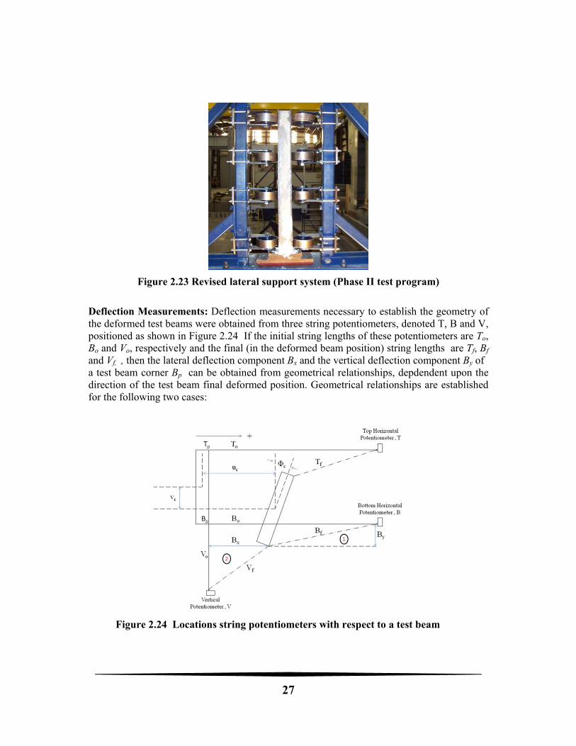
Although the distortion at the support regions occurring in the post-buckling stage had no effect on the buckling load nor on the deformation of the test beam prior to buckling, two additional casters on each side, supporting the bottom halves of the beam ends were used in the subsequent tests. Figure 2.23 shows the revised lateral support system that included four casters over the depth of the test beam.

Load Measurements: The load was measured by means of load calibrated load cells with compression capacities of 50 kips during Phase I and 100 kips during Phase II experimental program.

27

Figure 2.24 Locations string potentiometers with respect to a test beam

Figure 2.23 Revised lateral support system (Phase II test program)

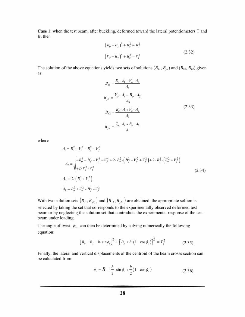
Deflection Measurements: Deflection measurements necessary to establish the geometry of the deformed test beams were obtained from three string potentiometers, denoted T, B and V, positioned as shown in Figure 2.24 If the initial string lengths of these potentiometers are To, Bo and Vo, respectively and the final (in the deformed beam position) string lengths are Tf, Bf and Vf, , then the lateral deflection component Bx and the vertical deflection component By of a test beam corner Bp can be obtained from geometrical relationships, depdendent upon the direction of the test beam final deformed position. Geometrical relationships are established for the following two cases:

28

Case 1: when the test beam, after buckling, deformed toward the lateral potentiometers T and B, then

2 2 2o x y fB B B B

2 2 2O y x fV B B V  

(2.32)

The solution of the above equations yields two sets of solutions (Bx1, By1) and (Bx2, By2) given as:

1 21

3

o ox

B A V AB

A

4 21

3

o oy

V A B AB

A

1 22

3

o ox

B A V AB

A

4 22

3

o oy

V A B AB

A

 

(2.33)

where

2 2 2 21 o o f fA B V B V

4 4 4 4 2 2 2 2 2 2 2

22 2

2 2

2

o f o f o f o f f o f

o f

B B V V B B V V B V VA

V V

2 23 2 o oB VA

2 2 2 2

4 o o f fA B V B V  

(2.34)

With two solution sets )11 , yx BB and )22 , yx BB are obtained, the appropriate soltion is

selected by taking the set that corresponds to the experimentally observed deformed test beam or by neglecting the solution set that contradicts the experimental response of the test beam under loading.

The angle of twist, c , can then be determined by solving numerically the following

equation:

222sin 1 coso x c y c fB B h B h T   (2.35)

Finally, the lateral and vertical displacements of the centroid of the beam crosss section can be calculated from:

sin 1 cos2 2

c x c c

h bu B

(2.36)

29

1 cos sin2 2

c y c c

h bv B  

Case 2: when the test beam, after buckling, deformed away from the lateral potentiometers T and B, then

2 2 2o x y fB B B B

2 2 2O y x fV B B V  

(2.37)

The soultion of the above equations yields either (Bx3, By3) or (Bx42, By4) given as:

1 23

3

o ox

B A V AB

A

4 23

3

o oy

V A B AB

A

1 24

3

o ox

B A V AB

A

4 24

3

o oy

V A B AB

A

 

(2.38)

After selecting the appropriate solution (Bx, By) that corresponds to the experimentally observed deflected test beam, the angle of twist, c , can be obtained by solving the following

equation:

222sin 1 coso x c y c fB B h B h T   (2.39)

The lateral and vertical displacements of the centroid of the beam cross section in this case are computed from:

sin 1 cos2 2

c x c c

h bu B

1 cos sin2 2

c y c c

h bv B  

(2.40)

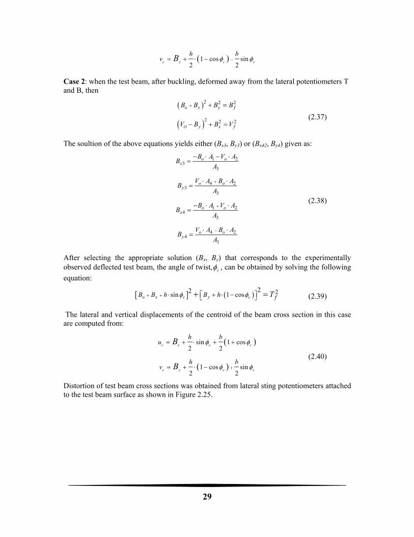
Distortion of test beam cross sections was obtained from lateral sting potentiometers attached to the test beam surface as shown in Figure 2.25.

30

Figure 2.26 Locations of LVDTs used for strain measurement in Phase I test program

Figure 2.25 Potentiometer positions for measuring cross section distortion

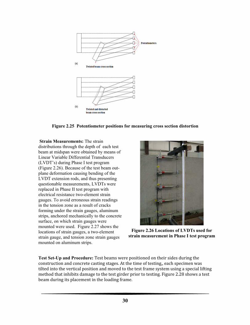
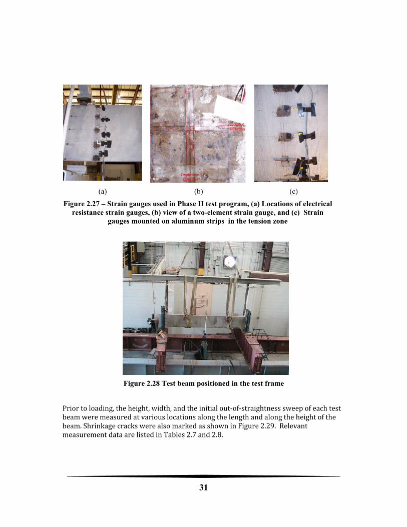
Strain Measurements: The strain distributions through the depth of each test beam at midspan were obtained by means of Linear Variable Differential Transducers (LVDT’s) during Phase I test program (Figure 2.26). Because of the test beam out-plane deformation causing bending of the LVDT extension rods, and thus presenting questionable measurements, LVDTs were replaced in Phase II test program with electrical resistance two-element strain gauges. To avoid erroneous strain readings in the tension zone as a result of cracks forming under the strain gauges, aluminum strips, anchored mechanically to the concrete surface, on which strain gauges were mounted were used. Figure 2.27 shows the locations of strain gauges, a two-element strain gauge, and tension zone strain gauges mounted on aluminum strips.

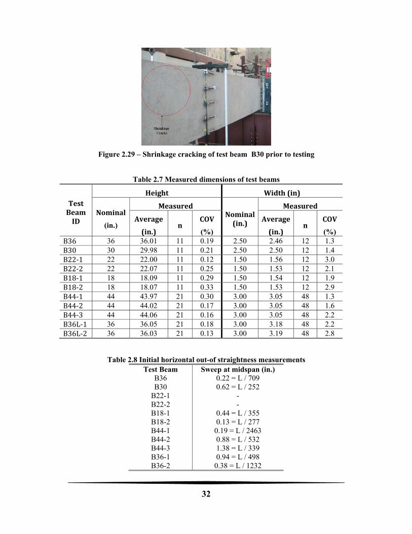
Test Set-Up and Procedure: Testbeamswerepositionedontheirsidesduringtheconstructionandconcretecastingstages.Atthetimeoftesting,,eachspecimenwastiltedintotheverticalpositionandmovedtothetestframesystemusingaspecialliftingmethodthatinhibitsdamagetothetestgirderpriortotesting.Figure2.28showsatestbeamduringitsplacementintheloadingframe.

31

(a) (b) (c)

Figure 2.27 – Strain gauges used in Phase II test program, (a) Locations of electrical resistance strain gauges, (b) view of a two-element strain gauge, and (c) Strain

gauges mounted on aluminum strips in the tension zone

Figure 2.28 Test beam positioned in the test frame

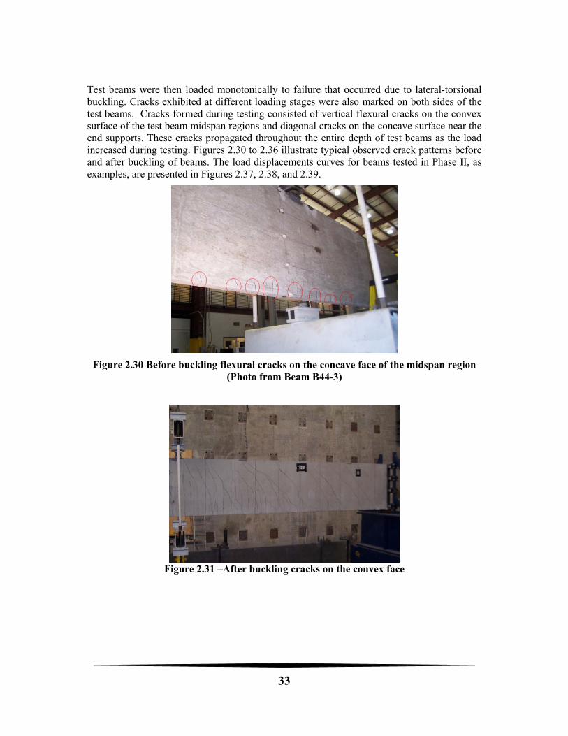
Priortoloading,theheight,width,andtheinitialout‐of‐straightnesssweepofeachtestbeamweremeasuredatvariouslocationsalongthelengthandalongtheheightofthebeam.ShrinkagecrackswerealsomarkedasshowninFigure2.29.RelevantmeasurementdataarelistedinTables2.7and2.8.

32

Figure 2.29 – Shrinkage cracking of test beam B30 prior to testing

Table 2.7 Measured dimensions of test beams

TestBeamID

Height Width(in)

Nominal

(in.)

MeasuredNominal(in.)

Measured

Average

(in.)n

COV

(%)

Average

(in.)n

COV

(%) B36 36 36.01 11 0.19 2.50 2.46 12 1.3 B30 30 29.98 11 0.21 2.50 2.50 12 1.4 B22‐1 22 22.00 11 0.12 1.50 1.56 12 3.0 B22‐2 22 22.07 11 0.25 1.50 1.53 12 2.1 B18‐1 18 18.09 11 0.29 1.50 1.54 12 1.9 B18‐2 18 18.07 11 0.33 1.50 1.53 12 2.9 B44‐1 44 43.97 21 0.30 3.00 3.05 48 1.3 B44‐2 44 44.02 21 0.17 3.00 3.05 48 1.6 B44‐3 44 44.06 21 0.16 3.00 3.05 48 2.2 B36L‐1 36 36.05 21 0.18 3.00 3.18 48 2.2 B36L‐2 36 36.03 21 0.13 3.00 3.19 48 2.8

Table 2.8 Initial horizontal out-of straightness measurements Test Beam Sweep at midspan (in.)

B36 0.22 = L / 709 B30 0.62 = L / 252

B22-1 - B22-2 - B18-1 0.44 = L / 355 B18-2 0.13 = L / 277 B44-1 0.19 = L / 2463 B44-2 0.88 = L / 532 B44-3 1.38 = L / 339 B36-1 0.94 = L / 498 B36-2 0.38 = L / 1232

33

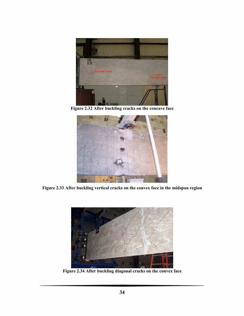
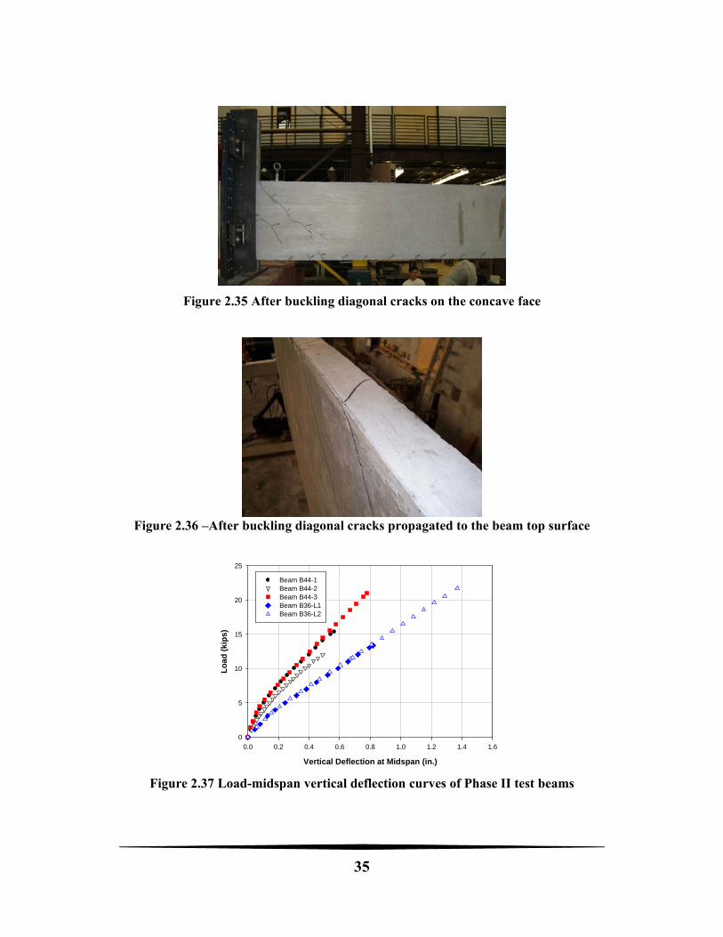
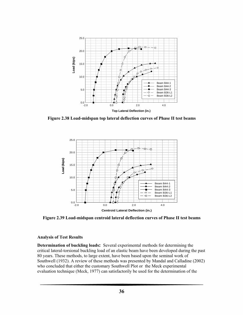
Test beams were then loaded monotonically to failure that occurred due to lateral-torsional buckling. Cracks exhibited at different loading stages were also marked on both sides of the test beams. Cracks formed during testing consisted of vertical flexural cracks on the convex surface of the test beam midspan regions and diagonal cracks on the concave surface near the end supports. These cracks propagated throughout the entire depth of test beams as the load increased during testing. Figures 2.30 to 2.36 illustrate typical observed crack patterns before and after buckling of beams. The load displacements curves for beams tested in Phase II, as examples, are presented in Figures 2.37, 2.38, and 2.39.

Figure 2.30 Before buckling flexural cracks on the concave face of the midspan region (Photo from Beam B44-3)

Figure 2.31 –After buckling cracks on the convex face

34

Figure 2.32 After buckling cracks on the concave face

Figure 2.33 After buckling vertical cracks on the convex face in the midspan region

Figure 2.34 After buckling diagonal cracks on the convex face

35

Figure 2.35 After buckling diagonal cracks on the concave face

Figure 2.36 –After buckling diagonal cracks propagated to the beam top surface

Vertical Deflection at Midspan (in.)

0.0 0.2 0.4 0.6 0.8 1.0 1.2 1.4 1.6

Lo

ad

(ki

ps)

0

5

10

15

20

25

Beam B44-1Beam B44-2Beam B44-3Beam B36-L1Beam B36-L2

Figure 2.37 Load-midspan vertical deflection curves of Phase II test beams

36

Top Lateral Deflection (in.)

-2.0 0.0 2.0 4.0

Lo

ad

(k

ips

)

0.0

5.0

10.0

15.0

20.0

25.0

Beam B44-1Beam B44-2 Beam B44-3 Beam B36-L1 Beam B36-L2

Figure 2.38 Load-midspan top lateral deflection curves of Phase II test beams

Centroid Lateral Deflection (in.)

-2.0 0.0 2.0 4.0

Load

(ki

ps)

0.0

5.0

10.0

15.0

20.0

25.0

Beam B44-1Beam B44-2 Beam B44-3 Beam B36-L1 Beam B36-L2

Figure 2.39 Load-midspan centroid lateral deflection curves of Phase II test beams

Analysis of Test Results

Determination of buckling loads: Several experimental methods for determining the critical lateral-torsional buckling load of an elastic beam have been developed during the past 80 years. These methods, to large extent, have been based upon the seminal work of Southwell (1932). A review of these methods was presented by Mandal and Calladine (2002) who concluded that either the customary Southwell Plot or the Meck experimental evaluation technique (Meck, 1977) can satisfactorily be used for the determination of the

37

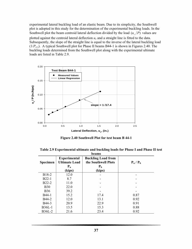
experimental lateral buckling load of an elastic beam. Due to its simplicity, the Southwell plot is adopted in this study for the determination of the experimental buckling loads. In the Southwell plot the beam centroid lateral deflection divided by the load )( Puc values are

plotted against the centroid lateral deflection uc and a straight line is fitted to the data. Subsequently, the slope of the straight line is equal to the inverse of the lateral buckling load (1/Pcr,). A typical Southwell plot for Phase II beams B44-1 is shown in Figures 2.40. The buckling loads determined from the Southwell plot along with the experimental ultimate loads are listed in Table 2.9.

Lateral Deflection, uc, (in.)

0.0 0.5 1.0 1.5 2.0 2.5

uc /

P (in

./ki

ps)

0.00

0.05

0.10

0.15

0.20

Measured ValuesLinear Regression

Test Beam B44-1

slope = 1 /17.4

Figure 2.40 Southwell Plot for test beam B 44-1

Table 2.9 Experimental ultimate and buckling loads for Phase I and Phase II test beams

Specimen Experimental Ultimate Load

Pu

Buckling Load from the Southwell Plots

Pb

Pu / Pb

(kips) (kips) B18-2 12.0 - - B22-1 8.7 - - B22-2 11.0 - - B30 22.0 - - B36 39.2 - -

B44-1 15.2 17.4 0.87 B44-2 12.0 13.1 0.92 B44-3 20.9 22.9 0.91

B36L-1 13.5 15.3 0.88 B36L-2 21.6 23.4 0.92

38

Torque at ultimate load: As shown in Table 2.10, the torque values, Teu , at the experimental ultimate load, approximately 10 to 15% of the buckling load, of all test beams are lower than those at which a reinforced concrete section cracks under torsion. Hsu (1968, 1993) found that the cracking torque of a solid reinforced concrete rectangular section correlates well with the following equation:

cp

cpccr p

AfT

2

5   (2.41)

However, for design purposes (ACI 2005) the cracking torque of a rectangular reinforced concrete section is evaluated from:

cp

cpccr p

AfT

2

4   (2.42)

in the above equations:

cpA = area enclosed by outside perimeter of concrete section, in.2

cpp = outside perimeter of concrete cross section, in.

cf = specified compressive strength of concrete, psi.

Table 2.10 Comparison of the torque at ultimate load vs. cracking torque

Specimen Torque at

Ultimate Load

euT

cp

cpccr p

AfT

2

5

cp

cpc

eu

p

Af

T2

5

cp

cpc

eu

p

Af

T2

4

(kip-in) (kip-in.) B44-1 50.6 88.0 0.58 0.73 B44-2 36.7 88.5 0.41 0.51 B44-3 38.0 88.7 0.42 0.53

B36L-1 47.7 74.4 0.64 0.80 B36L-2 46.2 75.0 0.62 0.78

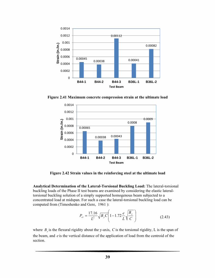
Concrete Compression Strain at ultimate load: The maximum compression strain values at the ultimate load of of each Phase II test beam are given in Figure 2.41.

Strain in the Reinforcing Steel at ultimate load: The measured strains of the reinforcing steel of Phase II test beams are presented in Figure 2.42. It is clearly shown that for all test beams, the reinforcing steel was in the elastic range ( ys ) when the buckling occurred.

39

Figure 2.41 Maximum concrete compression strain at the ultimate load

Figure 2.42 Strain values in the reinforcing steel at the ultimate load

Analytical Determination of the Lateral-Torsional Buckling Load: The lateral-torsional buckling loads of the Phase II test beams are examined by considering the elastic lateral-torsional buckling solution of a simply supported homogenous beam subjected to a concentrated load at midspan. For such a case the lateral-torsional buckling load can be computed from (Timoshenko and Gere, 1961 ):

C

B

L

eCB

LP y

ycr 72.1116.172

  (2.43)

where yB is the flexural rigidity about the y-axis, C is the torsional rigidity, L is the span of

the beam, and e is the vertical distance of the application of load from the centroid of the section.

0.000450.00038

0.00112

0.00041

0.00082

0

0.0002

0.0004

0.0006

0.0008

0.001

0.0012

0.0014

B44-1 B44-2 B44-3 B36L-1 B36L-2

Str

ain

(in

./in

.)

Test Beam

0.00065

0.00038 0.00043

0.00080.0009

0

0.0002

0.0004

0.0006

0.0008

0.001

0.0012

0.0014

B44-1 B44-2 B44-3 B36L-1 B36L-2

Str

ain

(in

./in

.)

Test Beam

40

In terms of the critical moment, equation 2.44 can be written as

C

B

L

eCB

LM y

ycr 72.1129.4

  (2.44)  

When the curvature about the major axis of bending is considered, equation 2.45 becomes (Vacharajittiphan et al., 1974):

xx

y

yy

cr

B

C

B

B

C

B

L

eCB

LM

11

72.1129.4

  (2.45)  

where xB is the flexural rigidity about the axis of bending x.

By neglecting the tension part of the concrete and denoting c for the depth of the compression part of the cross section, the flexural rigidities xB and yB , and the torsional rigidity C can be

computed from:

12

3bcEB cx   (2.46)

12

3cbEB cy   (2.47)

It is evident from equation 2.63 that lateral-torsional buckling will not occur for the case in which xy BB or alternatively 1cb . Thus it is sufficient to examine the lateral torsional

buckling case when 1cb for which the torsional rigidity can be computed as

c

bcbGC c 63.01

3

3

  (2.48)

Noting that with 2/ce , the term

C

B

L

e y72.11 will be close to one, approximating the

term cG with cE4.0 , and substituting Eqs. 2.46 and 2.47 into Eq. 2.45, the following

simplified equations are obtained:

c

b

c

b

c

b

c

bcb

L

EM c

cr

63.016.1

11

63.0145.0

2

2

2

2

3

 (2.49)

Eq. 2.49 can alternatively be written in the form:

41

c

b

c

b

c

b

c

b

cbE

LM

c

cr

63.016.1

11

63.0145.0

2

2

2

23 

(2.50)  

Using the minimum value of 3cbELM ccr , which is 0.44 when 14.0cb , the critical

moment can be given as

L

cbEM c

cr

344.0   (2.51)  

The above equation cannot be easily adopted for design purposes because the depth of the uncracked concrete portion, c , when buckling occurs is not known. Thus, the determination of crM will require iterations while maintaining the conditions of force equilibrium and strain

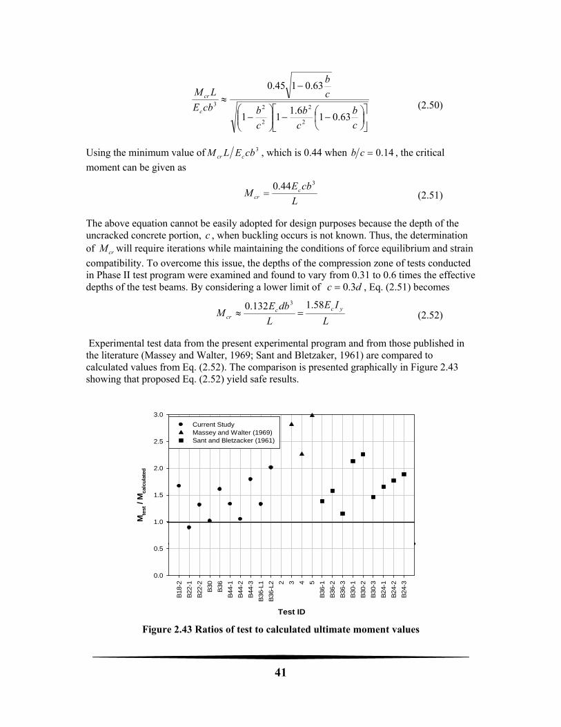
compatibility. To overcome this issue, the depths of the compression zone of tests conducted in Phase II test program were examined and found to vary from 0.31 to 0.6 times the effective depths of the test beams. By considering a lower limit of dc 3.0 , Eq. (2.51) becomes

L

IE

L

dbEM ycc

cr

58.1132.0 3

  (2.52)  

Experimental test data from the present experimental program and from those published in the literature (Massey and Walter, 1969; Sant and Bletzaker, 1961) are compared to calculated values from Eq. (2.52). The comparison is presented graphically in Figure 2.43 showing that proposed Eq. (2.52) yield safe results.

Proposed based on calculated critical moment

Test ID

B18-

2

B22-

1

B22-

2

B30

B36

B44-

1

B44-

2

B44-

3

B36

-L1

B36

-L2 2 3 4 5

B36-

1

B36-

2

B36-

3

B30-

1

B30-

2

B30-

3

B24-

1

B24-

2

B24-

3

Mte

st /

Mcalc

ula

ted

0.0

0.5

1.0

1.5

2.0

2.5

3.0

Current StudyMassey and Walter (1969)Sant and Bletzacker (1961)

Figure 2.43 Ratios of test to calculated ultimate moment values

42

2.3.6 Recommended Design Equation

For design purposes where reinforced concrete rectangular beams are subjected to a variety of loading cases, the critical moment as a result of lateral torsional buckling can be estimated from:

xx

y

y

bcr

B

C

B

B

CB

LCM

11

 

(2.53)  

where Cb is the moment modification factor for nonuniform moment diagrams when both ends of the unsupported segments are braced. Cb can conservatively be taken as unity, or calculated from:

.33435.2

5.12

max

max

CBA

b MMMM

MC   (2.54)  

and Mmax = absolute value of maximum moment in the unbraced segment MA = absolute value of moment at quarter point of the unbraced segment MB = absolute value of moment at the centerline of the unbraced segment MC = absolute value of moment at three-quarter point of the unbraced segment

Eq. (2.53) can be shown to take the form:

c

b

c

b

c

b

c

b

L

cbECM c

bcr

63.016.1

11

63.0133.0

2

2

2

2

3

 (2.55)

Using the minimum value of 3cbEC

LM

cb

cr , that is 0.323 when 14.0c

b , one can obtain:

L

cbECM c

bcr

332.0   (2.56)  

With dc 3.0 as found earlier, the critical moment can be expressed in the form:

L

IEC

L

dbEC

L

dbECM yc

bc

bc

bcr

2.1

10

0962.0 33

  (2.57)  

For the case of a simply supported beam subjected to a midspan concentrated load, Cb can be found to be equal to 1.32. When the value Cb=1.32 is substituted into Eq. 2.57, the result is identical to that of Eq. 2.52.

Based on the above results, one might establish the maximum unbraced length of a reinforced concrete beam, where lateral-torsional buckling limit state is not an issue, by requiring:

43

ncr MM   (2.58)  

where nM is the nominal flexural strength determined in accordance with the applicable

reinforced concrete design standards. When Eqs. (2.57) and (2.58) are combined, the maximum unbraced length can be computed from:

n

cb M

dbECL

10

3

  (2.59)  

44

45

CHAPTER 3

STABILITY OF PRESTRESSED CONCRETE BEAMS Six pretensioned rectangular sections were constructed for comparison with the nonprestressed reinforced concrete sections. The purposes were (1) to verify the theory that prestressing would not affect the theoretical lateral-stability critical moment and (2) to better understand the effect of initial imperfections. Background for Stability of Prestressed Concrete Beams Questions have been raised about the effect of the prestressing force. Would the prestressing cause a lower critical load like in the case of a steel beam-column or will the strands actually increase the critical load due to a restraint to lateral deformation from the strands? Would the prestressing force have any effect on the flexural and torsional rigidities? Several authors such as Magnel (1950), Billig (1953), and Leonhardt (1955) had come to the conclusion a prestressed concrete beam where the strands were bonded to the concrete cannot buckle. Billig (1953) stated that the prestressing force only would lead to a stability concern if the strands were unbonded over long distances. The reasoning behind not needing to perform stability calculations was due to the member being in equilibrium from the lateral reaction of the strand. Both Billig (1953) and Leondhardt (1955) cite Magnel (1944), in which Magnel’s (1950) book on prestressed concrete incorporated the results published in his 1944 journal article. Magnel (1950) used an example to analytically prove his theory. Magnel (1950) considered a beam with a prestressing tendon running through a duct sufficiently larger than the tendon where the tendon was rigidly attached only at the center by way of a cross-plate. Magnel (1950). Tests were done by Magnel (1950) to try to prove that a beam would not buckle by application of prestressing. The first of the relevant tests was performed on two concrete members that were 9.84 ft. (3 m) long with cross-sectional dimensions of 2 in. by 4 in. including a 5/8 in. longitudinal hole through the member. The first of the two members was tested with no prestressing wires and buckled at a load of 10,600 lbs. The achieved buckling load was very close to the theoretical Euler buckling load for the member. The second specimen was prestressed with four 0.2 in. wires and loaded to 19,000 lbs. with no signs of instability or failure of the concrete at that load. The second relevant test was performed on a concrete member with a length of 20 ft. with a cross-section that was 4 in. by 4 in. A 1.5 in. longitudinal hole was provided for a cable constructed of sixteen 0.2 in. wires. These dimensions and material properties would give a buckling load of 14,100 lbs. according to the Belgium regulations to which Magnel (1950) referred. The prestressing wires were stressed two at a time until the load was 49,400 lbs. No sign of instability or of concrete crushing was initially noticeable but after five minutes, the concrete failed in compression. The prestressed member had a slenderness ratio of 185 but had the failure load that would normally be representative of a member with a slenderness ratio of 14. Magnel (1950) believed that these test results confirmed the theory that a

46

member with prestressing tendons continuously in contact with the concrete would not buckle. Molke (1956). This paper discussed a specific case study of a high school auditorium in Springfield, Missouri that was framed with 146 ft. prestressed roof girders. The prestressed roof girders needed special investigation of their stability while being lifted and placed before there was bracing from the roof slabs. In literature, it was well established that with straight or curved concrete columns, there was no concern with respect to stability failure as long as the prestressing strands were located at the centroid of the section according to Molke (1956). Any bending moment created by the prestressing force in the strands would then be countered by an equal and opposite restoring force. Molke (1956) believed this had often been misconstrued to mean there was never any stability concern in prestressed concrete members. Any externally applied loads on the member could produce the same type of buckling failures as considered if the member had not been prestressed. Furthermore, the buckling load could actually be considered to be less than typical since the prestressing force would reduce the elastic modulus of the concrete. The girders in question for the auditorium roof had sufficient factor of safety when utilizing traditional formulas for lateral buckling of beams. Molke (1956) believed that proof of a minimum factor of safety for buckling in concrete structures should be calculated based on elastic theory and should be a code requirement. Stafford (1999). Stratford used classical stability theory and did not consider prestressed concrete girders differently in any way. Both Muller (1962) and Stratford (1999) also considered classical stability theory of a hanging girder, and Stratford (1999) considered imperfections extensively. Stratford (2000) expanded the work on hanging girders by considering the girder deformations as a rigid body rotation (infinite torsion constant) and a lateral deflection. König and Pauli (1990). They tested six non-prestressed and prestressed I and T shaped sections. All of the specimens underwent the same unstable failure mechanism. As the transverse load increased, lateral deflections did so at a relatively small amount; however, when the critical load was reached, lateral deflections increased at a large magnitude, and there was very little load increase after the critical load was reached. The damage to the beams after the tests included diagonal cracks that developed on both the convex and concave sides of the specimens, and the cracks on the convex side of the specimens were perpendicular to those on the concave side. This type of diagonal cracking is representative of torsion cracking in reinforced concrete beams and is an indicator of lateral-torsional buckling. Furthermore, it was noted by König and Pauli (1990) that amount of cracking was less on the concave side relative to the convex side, particularly in the case of the two prestressed beams. That makes intuitive sense because there is compression on the concave side due to weak-axis bending that acts to close the torsional cracks on that side; however, on the convex side, there is tension from the weak-axis bending that acts to amplify the torsional cracking on that side. It is important to note that weak-axis bending stresses and the torsional stresses were developed in the experiments by König and Pauli (1990) due to the end restraints. The end conditions that they used were: torsional restraint, vertical translation restraint, horizontal translation restraint, free rotation about horizontal axis and free rotation about vertical axis.

47

The results indicated that both widening the top flange and adding additional compression reinforcement increase the stability of the cross-section. Furthermore, the prestressing force did not produce any significant effect with respect to the specimens’ stability because the nonprestressed and prestressed sections were the same with respect to geometry, and amount and location of reinforcing steel; the critical loads for the prestressed section was only 16% greater than for the nonprestressed section. Experimental Approach The six beams had a length of 32 ft., a width of 4 in. and a height of 40 in. The dimensions of these beams gave a span/width ratio of 93 and a depth/width ratio of 9.5. The reasons for the dimensions initially resulted from the selection of the width of the beams. The width was selected to be as small a possible to create a large slenderness. A width of 4 in. was the smallest that could be made by the precast plant and still guarantee the prestressing would be able to be properly done; and furthermore, assure no damage during the handling of the test beams. From the width, the length was determined by the need of a large span/width ratio, and the specific dimensional constraints allowed by the anchoring grid in the floor at the Georgia Institute of Technology Structural Engineering Laboratory. The depth was selected such that it would create the largest possible depth/width ratio, while being shallow enough that cracking would not occur when being tipped up from their sides after fabrication. The geometric ratios were compared with those of the reinforced concrete test specimens from Revathi and Menon (2003), and both ratios were found to be greater; and therefore, more slender than the beams tested by Revathi and Menon (2003), in which all of their test specimens buckled. The six rectangular beams were split into three pairs. Each pair had a different prestressing strand pattern, but the same amount of mild steel reinforcement and approximate location of the mild steel reinforcement. The three different prestressing cases were: two strands located at the centroid of the cross-section (40C2), two strands located at the bottom of the cross-section (40B2) and one strand located at the bottom of the cross-section (40B1). The strand patterns were selected such that the effect of strand location (eccentricity) was determined from a comparison of beams 40C2 and 40B2, because the prestressing force was approximately the same, but strand location was not. Furthermore, the effect of prestressing force was determined from a comparison of beams 40B2 and 40B1, because the strand locations were approximately the same, but the prestressing force was significantly different.

The usefulness of the six rectangular beams lies in the experimental verification of the lateral-torsional buckling behavior of prestressed concrete beams, and allows for the validation of existing analytical methods, or creation of a new analytical method, while initially using a simple geometry. Experimental methods were similar to those used for the nonprestressed sections except that the span length was greater and a larger capacity gravity load simulator was used. The seventh specimen was a 101 ft. PCI BT-54 bridge girder. The BT-54 was prestressed with 40 – 0.6” diameter prestressing strands with each strand having a jacking force of 43,943 lbs.

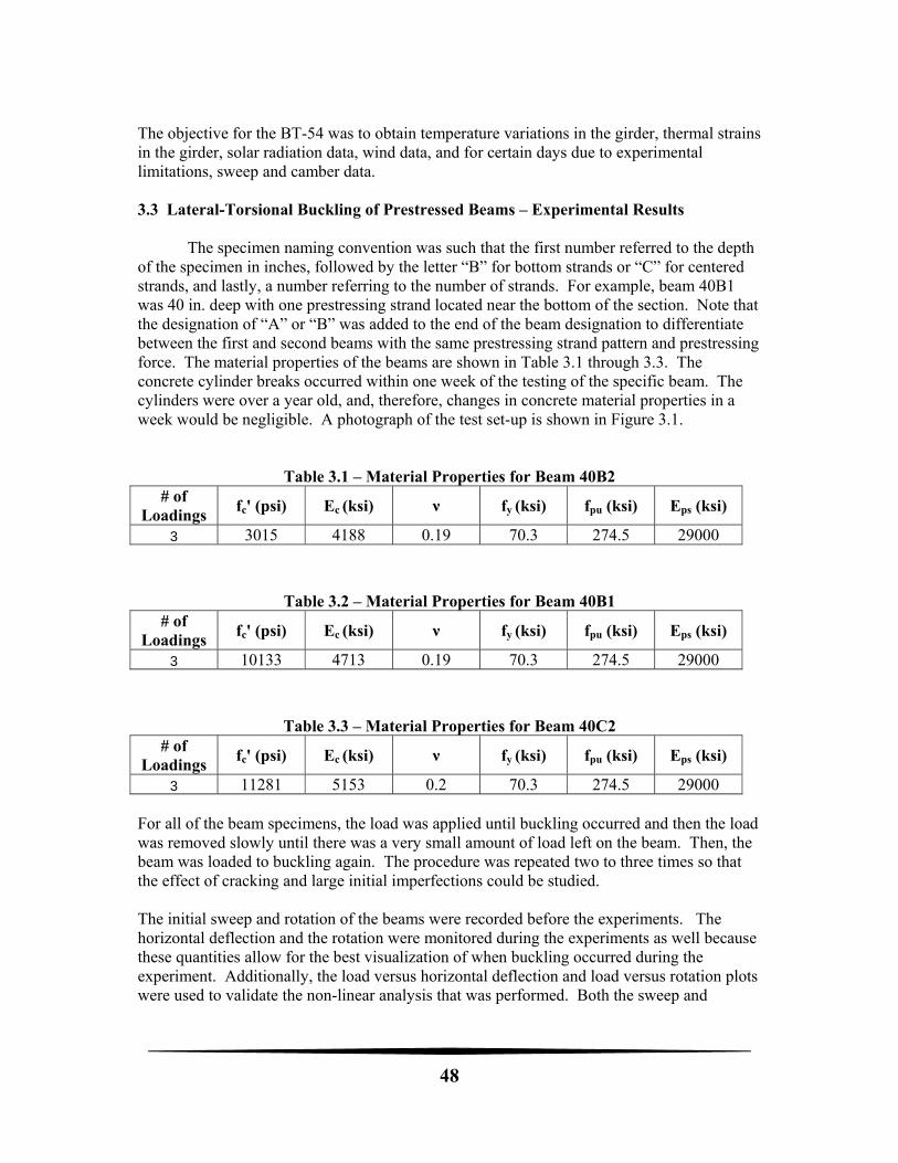
48

The objective for the BT-54 was to obtain temperature variations in the girder, thermal strains in the girder, solar radiation data, wind data, and for certain days due to experimental limitations, sweep and camber data. 3.3 Lateral-Torsional Buckling of Prestressed Beams – Experimental Results The specimen naming convention was such that the first number referred to the depth of the specimen in inches, followed by the letter “B” for bottom strands or “C” for centered strands, and lastly, a number referring to the number of strands. For example, beam 40B1 was 40 in. deep with one prestressing strand located near the bottom of the section. Note that the designation of “A” or “B” was added to the end of the beam designation to differentiate between the first and second beams with the same prestressing strand pattern and prestressing force. The material properties of the beams are shown in Table 3.1 through 3.3. The concrete cylinder breaks occurred within one week of the testing of the specific beam. The cylinders were over a year old, and, therefore, changes in concrete material properties in a week would be negligible. A photograph of the test set-up is shown in Figure 3.1.

Table 3.1 – Material Properties for Beam 40B2 # of

Loadings fc' (psi) Ec (ksi) ν fy (ksi) fpu (ksi) Eps (ksi)

3 3015 4188 0.19 70.3 274.5 29000

Table 3.2 – Material Properties for Beam 40B1 # of

Loadings fc' (psi) Ec (ksi) ν fy (ksi) fpu (ksi) Eps (ksi)

3 10133 4713 0.19 70.3 274.5 29000

Table 3.3 – Material Properties for Beam 40C2 # of

Loadings fc' (psi) Ec (ksi) ν fy (ksi) fpu (ksi) Eps (ksi)

3 11281 5153 0.2 70.3 274.5 29000 For all of the beam specimens, the load was applied until buckling occurred and then the load was removed slowly until there was a very small amount of load left on the beam. Then, the beam was loaded to buckling again. The procedure was repeated two to three times so that the effect of cracking and large initial imperfections could be studied. The initial sweep and rotation of the beams were recorded before the experiments. The horizontal deflection and the rotation were monitored during the experiments as well because these quantities allow for the best visualization of when buckling occurred during the experiment. Additionally, the load versus horizontal deflection and load versus rotation plots were used to validate the non-linear analysis that was performed. Both the sweep and

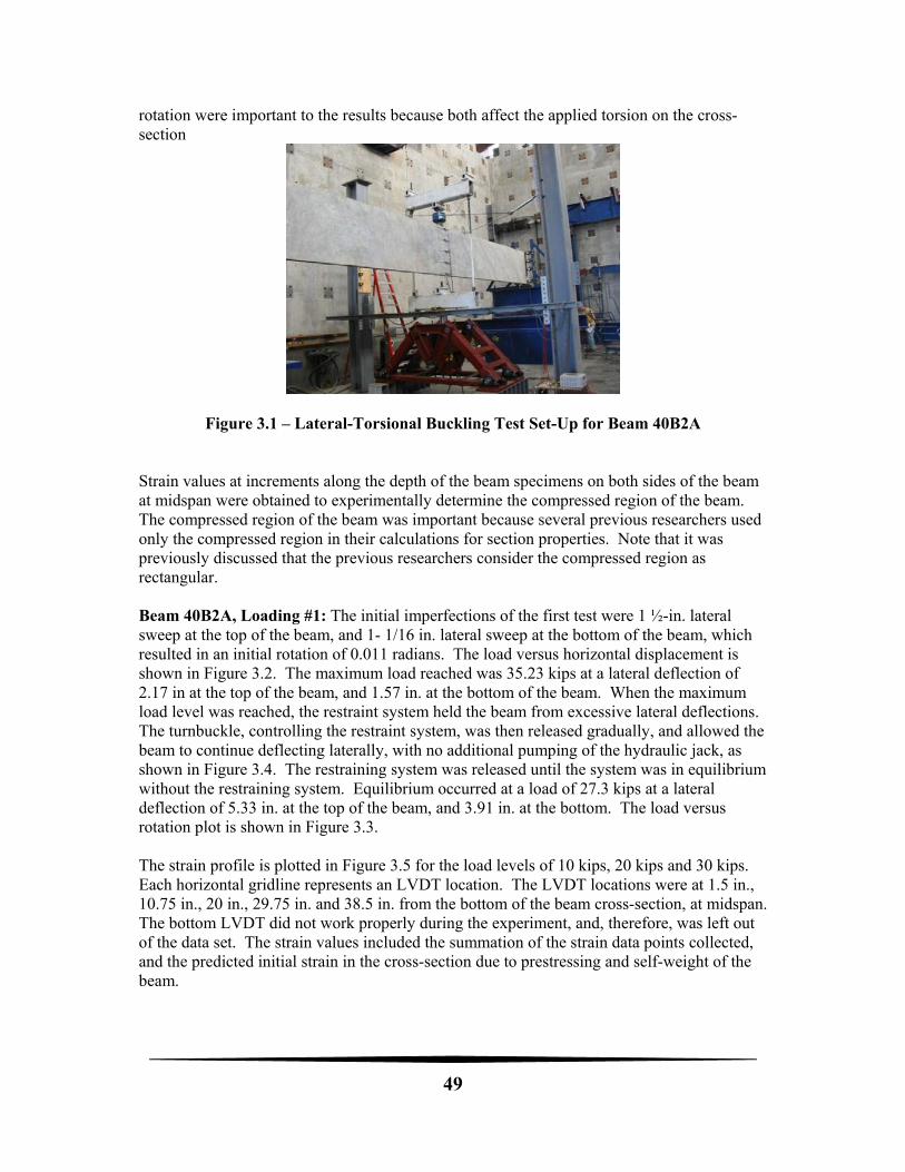
49

rotation were important to the results because both affect the applied torsion on the cross-section

Figure 3.1 – Lateral-Torsional Buckling Test Set-Up for Beam 40B2A

Strain values at increments along the depth of the beam specimens on both sides of the beam at midspan were obtained to experimentally determine the compressed region of the beam. The compressed region of the beam was important because several previous researchers used only the compressed region in their calculations for section properties. Note that it was previously discussed that the previous researchers consider the compressed region as rectangular. Beam 40B2A, Loading #1: The initial imperfections of the first test were 1 ½-in. lateral sweep at the top of the beam, and 1- 1/16 in. lateral sweep at the bottom of the beam, which resulted in an initial rotation of 0.011 radians. The load versus horizontal displacement is shown in Figure 3.2. The maximum load reached was 35.23 kips at a lateral deflection of 2.17 in at the top of the beam, and 1.57 in. at the bottom of the beam. When the maximum load level was reached, the restraint system held the beam from excessive lateral deflections. The turnbuckle, controlling the restraint system, was then released gradually, and allowed the beam to continue deflecting laterally, with no additional pumping of the hydraulic jack, as shown in Figure 3.4. The restraining system was released until the system was in equilibrium without the restraining system. Equilibrium occurred at a load of 27.3 kips at a lateral deflection of 5.33 in. at the top of the beam, and 3.91 in. at the bottom. The load versus rotation plot is shown in Figure 3.3. The strain profile is plotted in Figure 3.5 for the load levels of 10 kips, 20 kips and 30 kips. Each horizontal gridline represents an LVDT location. The LVDT locations were at 1.5 in., 10.75 in., 20 in., 29.75 in. and 38.5 in. from the bottom of the beam cross-section, at midspan. The bottom LVDT did not work properly during the experiment, and, therefore, was left out of the data set. The strain values included the summation of the strain data points collected, and the predicted initial strain in the cross-section due to prestressing and self-weight of the beam.

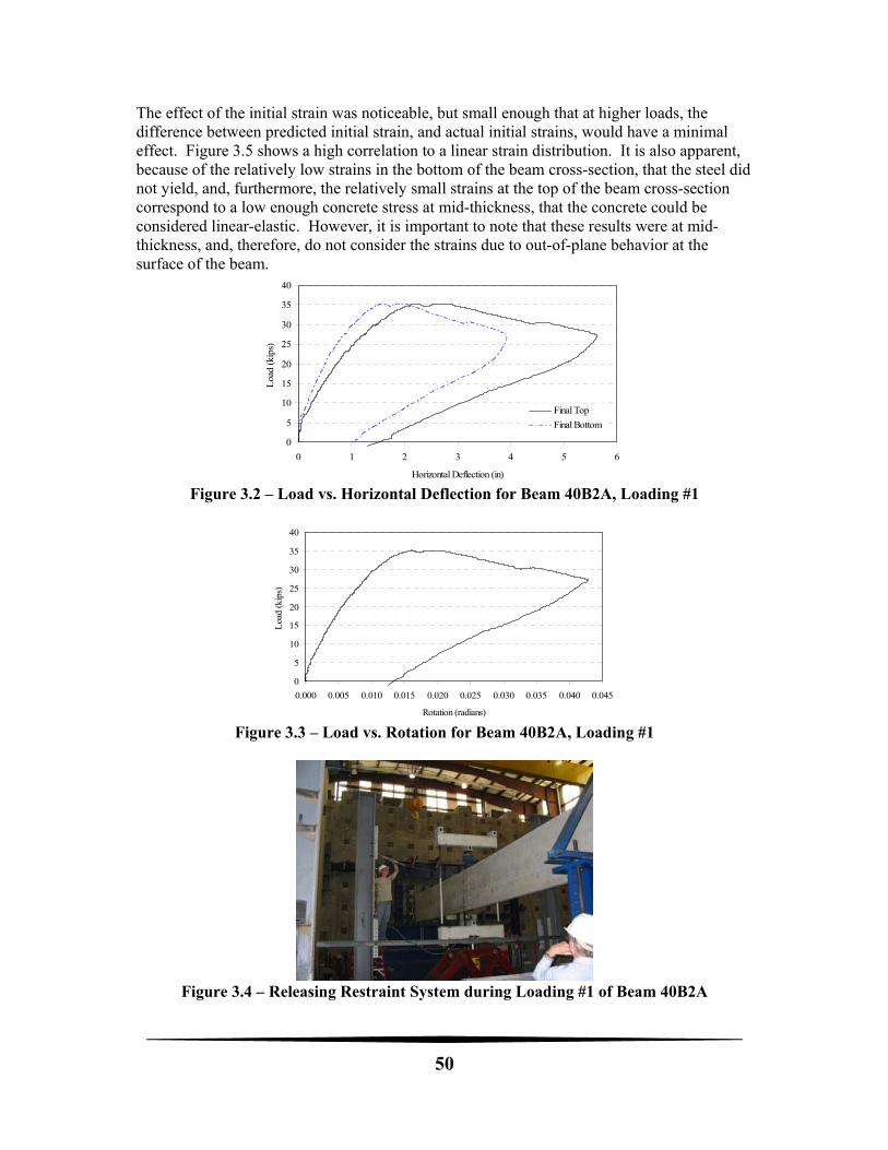
50

The effect of the initial strain was noticeable, but small enough that at higher loads, the difference between predicted initial strain, and actual initial strains, would have a minimal effect. Figure 3.5 shows a high correlation to a linear strain distribution. It is also apparent, because of the relatively low strains in the bottom of the beam cross-section, that the steel did not yield, and, furthermore, the relatively small strains at the top of the beam cross-section correspond to a low enough concrete stress at mid-thickness, that the concrete could be considered linear-elastic. However, it is important to note that these results were at mid-thickness, and, therefore, do not consider the strains due to out-of-plane behavior at the surface of the beam.

Figure 3.2 – Load vs. Horizontal Deflection for Beam 40B2A, Loading #1

Figure 3.3 – Load vs. Rotation for Beam 40B2A, Loading #1

Figure 3.4 – Releasing Restraint System during Loading #1 of Beam 40B2A

0

5

10

15

20

25

30

35

40

0 1 2 3 4 5 6

Horizontal Deflection (in)

Loa

d (k

ips)

Final Top

Final Bottom

0

5

10

15

20

25

30

35

40

0.000 0.005 0.010 0.015 0.020 0.025 0.030 0.035 0.040 0.045

Rotation (radians)

Loa

d (k

ips)

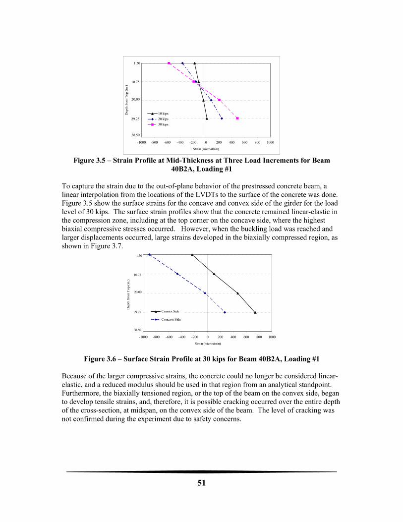
51

Figure 3.5 – Strain Profile at Mid-Thickness at Three Load Increments for Beam

40B2A, Loading #1 To capture the strain due to the out-of-plane behavior of the prestressed concrete beam, a linear interpolation from the locations of the LVDTs to the surface of the concrete was done. Figure 3.5 show the surface strains for the concave and convex side of the girder for the load level of 30 kips. The surface strain profiles show that the concrete remained linear-elastic in the compression zone, including at the top corner on the concave side, where the highest biaxial compressive stresses occurred. However, when the buckling load was reached and larger displacements occurred, large strains developed in the biaxially compressed region, as shown in Figure 3.7.

Figure 3.6 – Surface Strain Profile at 30 kips for Beam 40B2A, Loading #1

Because of the larger compressive strains, the concrete could no longer be considered linear-elastic, and a reduced modulus should be used in that region from an analytical standpoint. Furthermore, the biaxially tensioned region, or the top of the beam on the convex side, began to develop tensile strains, and, therefore, it is possible cracking occurred over the entire depth of the cross-section, at midspan, on the convex side of the beam. The level of cracking was not confirmed during the experiment due to safety concerns.

-1000 -800 -600 -400 -200 0 200 400 600 800 1000

Strain (microstrain)

Dep

th f

rom

Top

(in

.)

10 kips

20 kips

30 kips

1.50

10.75

38.50

29.25

20.00

-1000 -800 -600 -400 -200 0 200 400 600 800 1000

Strain (microstrain)

Dep

th f

rom

Top

(in

.)

Convex Side

Concave Side

1.50

10.75

38.50

29.25

20.00

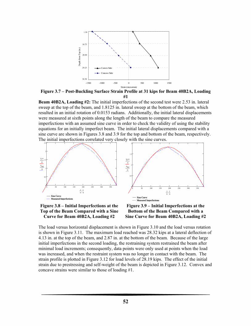
52

Figure 3.7 – Post-Buckling Surface Strain Profile at 31 kips for Beam 40B2A, Loading

#1 Beam 40B2A, Loading #2: The initial imperfections of the second test were 2.53 in. lateral sweep at the top of the beam, and 1.8125 in. lateral sweep at the bottom of the beam, which resulted in an initial rotation of 0.0153 radians. Additionally, the initial lateral displacements were measured at sixth points along the length of the beam to compare the measured imperfections with an assumed sine curve in order to check the validity of using the stability equations for an initially imperfect beam. The initial lateral displacements compared with a sine curve are shown in Figures 3.8 and 3.9 for the top and bottom of the beam, respectively. The initial imperfections correlated very closely with the sine curves.

Figure 3.8 – Initial Imperfections at the Top of the Beam Compared with a Sine

Curve for Beam 40B2A, Loading #2

Figure 3.9 – Initial Imperfections at the Bottom of the Beam Compared with a

Sine Curve for Beam 40B2A, Loading #2 The load versus horizontal displacement is shown in Figure 3.10 and the load versus rotation is shown in Figure 3.11. The maximum load reached was 28.32 kips at a lateral deflection of 4.13 in. at the top of the beam, and 2.87 in. at the bottom of the beam. Because of the large initial imperfections in the second loading, the restraining system restrained the beam after minimal load increments; consequently, data points were only used at points when the load was increased, and when the restraint system was no longer in contact with the beam. The strain profile is plotted in Figure 3.12 for load levels of 28.19 kips. The effect of the initial strain due to prestressing and self-weight of the beam is depicted in Figure 3.12. Convex and concave strains were similar to those of loading #1.

-1500 -1000 -500 0 500 1000 1500

Strain (microstrain)

Dep

th f

rom

Top

(in

.)

Convex Side

Concave Side

1.50

10.75

38.50

29.25

20.00

0 50 100 150 200 250 300 3500

0.5

1

1.5

2

2.5

Sine CurveMeasured ImperfectionsSine CurveMeasured Imperfections

ft x( )

in

top

in

x

in

z

in

0 50 100 150 200 250 300 3500

0.5

1

1.5

2

Sine CurveMeasured ImperfectionsSine CurveMeasured Imperfections

fb x( )

in

bot

in

x

in

z

in

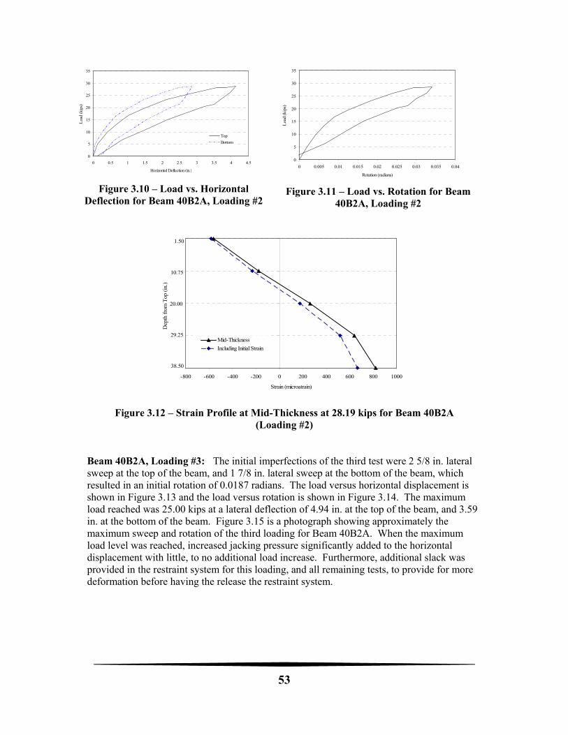
53

Figure 3.10 – Load vs. Horizontal Deflection for Beam 40B2A, Loading #2

Figure 3.11 – Load vs. Rotation for Beam 40B2A, Loading #2

Figure 3.12 – Strain Profile at Mid-Thickness at 28.19 kips for Beam 40B2A (Loading #2)

Beam 40B2A, Loading #3: The initial imperfections of the third test were 2 5/8 in. lateral sweep at the top of the beam, and 1 7/8 in. lateral sweep at the bottom of the beam, which resulted in an initial rotation of 0.0187 radians. The load versus horizontal displacement is shown in Figure 3.13 and the load versus rotation is shown in Figure 3.14. The maximum load reached was 25.00 kips at a lateral deflection of 4.94 in. at the top of the beam, and 3.59 in. at the bottom of the beam. Figure 3.15 is a photograph showing approximately the maximum sweep and rotation of the third loading for Beam 40B2A. When the maximum load level was reached, increased jacking pressure significantly added to the horizontal displacement with little, to no additional load increase. Furthermore, additional slack was provided in the restraint system for this loading, and all remaining tests, to provide for more deformation before having the release the restraint system.

0

5

10

15

20

25

30

35

0 0.5 1 1.5 2 2.5 3 3.5 4 4.5

Horizontal Deflection (in.)

Loa

d (k

ips)

Top

Bottom

0

5

10

15

20

25

30

35

0 0.005 0.01 0.015 0.02 0.025 0.03 0.035 0.04

Rotation (radians)

Loa

d (k

ips)

-800 -600 -400 -200 0 200 400 600 800 1000

Strain (microatrain)

Dep

th f

rom

Top

(in

.)

Mid-Thickness

Including Initial Strain

1.50

10.75

38.50

29.25

20.00

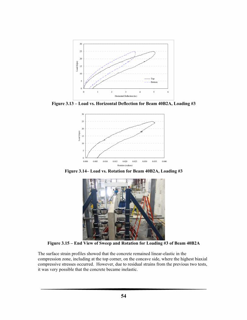
54

Figure 3.13 – Load vs. Horizontal Deflection for Beam 40B2A, Loading #3

Figure 3.14– Load vs. Rotation for Beam 40B2A, Loading #3

Figure 3.15 – End View of Sweep and Rotation for Loading #3 of Beam 40B2A

The surface strain profiles showed that the concrete remained linear-elastic in the compression zone, including at the top corner, on the concave side, where the highest biaxial compressive stresses occurred. However, due to residual strains from the previous two tests, it was very possible that the concrete became inelastic.

0

5

10

15

20

25

30

0 1 2 3 4 5 6

Horizontal Deflection (in.)

Loa

d (k

ips)

Top

Bottom

0

5

10

15

20

25

30

0.000 0.005 0.010 0.015 0.020 0.025 0.030 0.035 0.040

Rotation (radians)

Loa

d (k

ips)

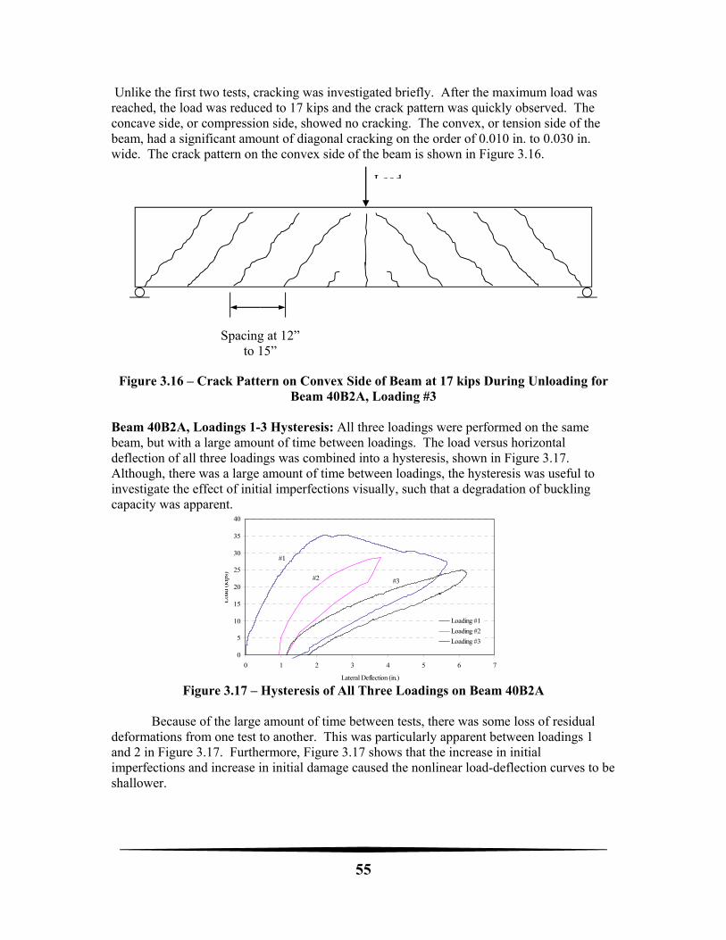
55

Unlike the first two tests, cracking was investigated briefly. After the maximum load was reached, the load was reduced to 17 kips and the crack pattern was quickly observed. The concave side, or compression side, showed no cracking. The convex, or tension side of the beam, had a significant amount of diagonal cracking on the order of 0.010 in. to 0.030 in. wide. The crack pattern on the convex side of the beam is shown in Figure 3.16.

Figure 3.16 – Crack Pattern on Convex Side of Beam at 17 kips During Unloading for

Beam 40B2A, Loading #3

Beam 40B2A, Loadings 1-3 Hysteresis: All three loadings were performed on the same beam, but with a large amount of time between loadings. The load versus horizontal deflection of all three loadings was combined into a hysteresis, shown in Figure 3.17. Although, there was a large amount of time between loadings, the hysteresis was useful to investigate the effect of initial imperfections visually, such that a degradation of buckling capacity was apparent.

Figure 3.17 – Hysteresis of All Three Loadings on Beam 40B2A

Because of the large amount of time between tests, there was some loss of residual deformations from one test to another. This was particularly apparent between loadings 1 and 2 in Figure 3.17. Furthermore, Figure 3.17 shows that the increase in initial imperfections and increase in initial damage caused the nonlinear load-deflection curves to be shallower.

0

5

10

15

20

25

30

35

40

0 1 2 3 4 5 6 7

Lateral Deflection (in.)

Loa

d (k

ips)

Loading #1

Loading #2

Loading #3

#2 #3

#1

Load

Spacing at 12” to 15”

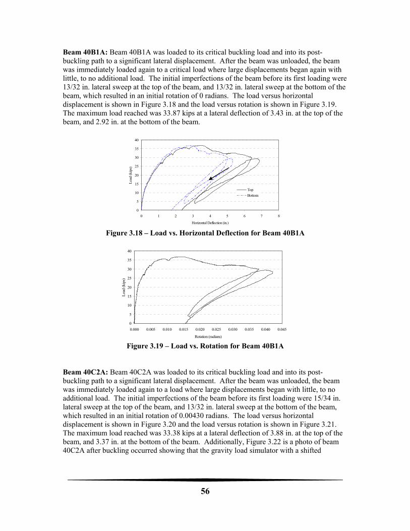
56

Beam 40B1A: Beam 40B1A was loaded to its critical buckling load and into its post-buckling path to a significant lateral displacement. After the beam was unloaded, the beam was immediately loaded again to a critical load where large displacements began again with little, to no additional load. The initial imperfections of the beam before its first loading were 13/32 in. lateral sweep at the top of the beam, and 13/32 in. lateral sweep at the bottom of the beam, which resulted in an initial rotation of 0 radians. The load versus horizontal displacement is shown in Figure 3.18 and the load versus rotation is shown in Figure 3.19. The maximum load reached was 33.87 kips at a lateral deflection of 3.43 in. at the top of the beam, and 2.92 in. at the bottom of the beam.

Figure 3.18 – Load vs. Horizontal Deflection for Beam 40B1A

Figure 3.19 – Load vs. Rotation for Beam 40B1A

Beam 40C2A: Beam 40C2A was loaded to its critical buckling load and into its post-buckling path to a significant lateral displacement. After the beam was unloaded, the beam was immediately loaded again to a load where large displacements began with little, to no additional load. The initial imperfections of the beam before its first loading were 15/34 in. lateral sweep at the top of the beam, and 13/32 in. lateral sweep at the bottom of the beam, which resulted in an initial rotation of 0.00430 radians. The load versus horizontal displacement is shown in Figure 3.20 and the load versus rotation is shown in Figure 3.21. The maximum load reached was 33.38 kips at a lateral deflection of 3.88 in. at the top of the beam, and 3.37 in. at the bottom of the beam. Additionally, Figure 3.22 is a photo of beam 40C2A after buckling occurred showing that the gravity load simulator with a shifted

0

5

10

15

20

25

30

35

40

0 1 2 3 4 5 6 7 8

Horizontal Deflection (in.)

Loa

d (k

ips)

Top

Bottom

0

5

10

15

20

25

30

35

40

0.000 0.005 0.010 0.015 0.020 0.025 0.030 0.035 0.040 0.045

Rotation (radians)

Loa

d (k

ips)

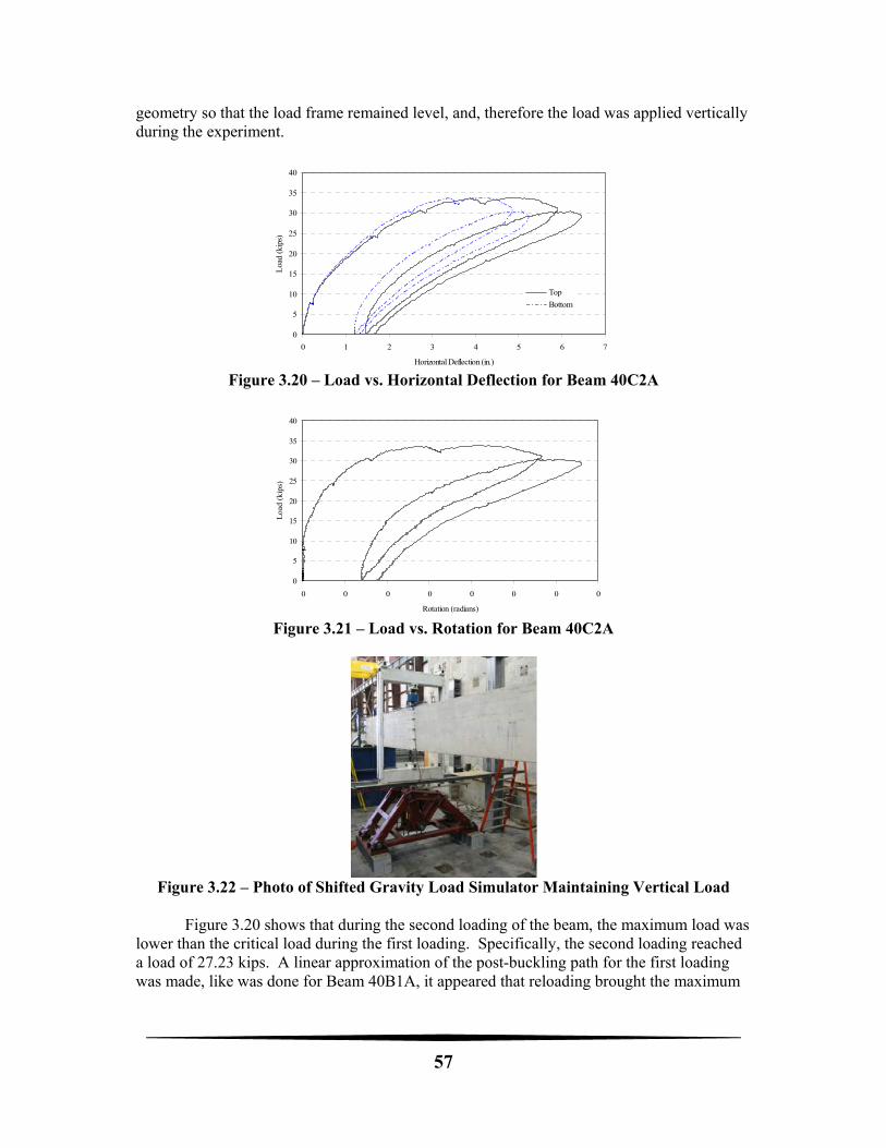
57

geometry so that the load frame remained level, and, therefore the load was applied vertically during the experiment.

Figure 3.20 – Load vs. Horizontal Deflection for Beam 40C2A

Figure 3.21 – Load vs. Rotation for Beam 40C2A

Figure 3.22 – Photo of Shifted Gravity Load Simulator Maintaining Vertical Load

Figure 3.20 shows that during the second loading of the beam, the maximum load was lower than the critical load during the first loading. Specifically, the second loading reached a load of 27.23 kips. A linear approximation of the post-buckling path for the first loading was made, like was done for Beam 40B1A, it appeared that reloading brought the maximum

0

5

10

15

20

25

30

35

40

0 1 2 3 4 5 6 7

Horizontal Deflection (in.)

Loa

d (k

ips)

Top

Bottom

0

5

10

15

20

25

30

35

40

0 0 0 0 0 0 0 0

Rotation (radians)

Loa

d (k

ips)

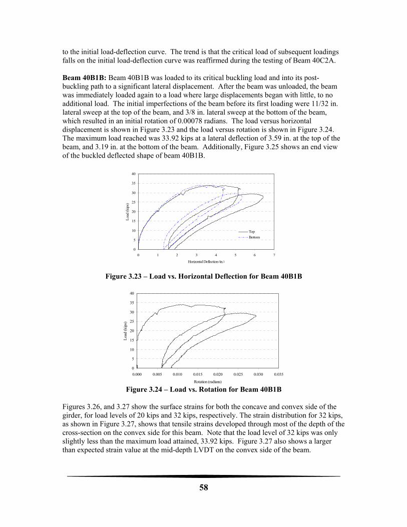
58

to the initial load-deflection curve. The trend is that the critical load of subsequent loadings falls on the initial load-deflection curve was reaffirmed during the testing of Beam 40C2A. Beam 40B1B: Beam 40B1B was loaded to its critical buckling load and into its post-buckling path to a significant lateral displacement. After the beam was unloaded, the beam was immediately loaded again to a load where large displacements began with little, to no additional load. The initial imperfections of the beam before its first loading were 11/32 in. lateral sweep at the top of the beam, and 3/8 in. lateral sweep at the bottom of the beam, which resulted in an initial rotation of 0.00078 radians. The load versus horizontal displacement is shown in Figure 3.23 and the load versus rotation is shown in Figure 3.24. The maximum load reached was 33.92 kips at a lateral deflection of 3.59 in. at the top of the beam, and 3.19 in. at the bottom of the beam. Additionally, Figure 3.25 shows an end view of the buckled deflected shape of beam 40B1B.

Figure 3.23 – Load vs. Horizontal Deflection for Beam 40B1B

Figure 3.24 – Load vs. Rotation for Beam 40B1B

Figures 3.26, and 3.27 show the surface strains for both the concave and convex side of the girder, for load levels of 20 kips and 32 kips, respectively. The strain distribution for 32 kips, as shown in Figure 3.27, shows that tensile strains developed through most of the depth of the cross-section on the convex side for this beam. Note that the load level of 32 kips was only slightly less than the maximum load attained, 33.92 kips. Figure 3.27 also shows a larger than expected strain value at the mid-depth LVDT on the convex side of the beam.

0

5

10

15

20

25

30

35

40

0 1 2 3 4 5 6 7

Horizontal Deflection (in.)

Loa

d (k

ips)

Top

Bottom

0

5

10

15

20

25

30

35

40

0.000 0.005 0.010 0.015 0.020 0.025 0.030 0.035

Rotation (radians)

Loa

d (k

ips)

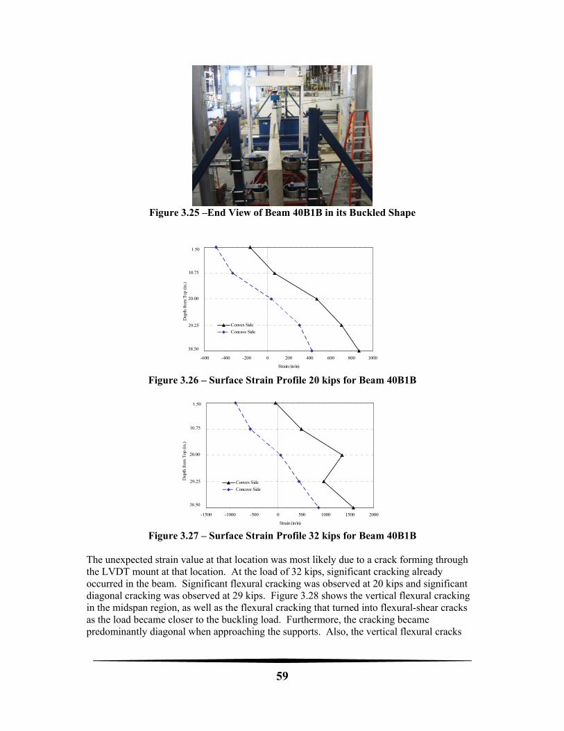
59

Figure 3.25 –End View of Beam 40B1B in its Buckled Shape

Figure 3.26 – Surface Strain Profile 20 kips for Beam 40B1B

Figure 3.27 – Surface Strain Profile 32 kips for Beam 40B1B

The unexpected strain value at that location was most likely due to a crack forming through the LVDT mount at that location. At the load of 32 kips, significant cracking already occurred in the beam. Significant flexural cracking was observed at 20 kips and significant diagonal cracking was observed at 29 kips. Figure 3.28 shows the vertical flexural cracking in the midspan region, as well as the flexural cracking that turned into flexural-shear cracks as the load became closer to the buckling load. Furthermore, the cracking became predominantly diagonal when approaching the supports. Also, the vertical flexural cracks

-600 -400 -200 0 200 400 600 800 1000

Strain (in/in)

Dep

th f

rom

Top

(in

.)

Convex Side

Concave Side

1.50

10.75

38.50

29.25

20.00

-1500 -1000 -500 0 500 1000 1500 2000

Strain (in/in)

Dep

th f

rom

Top

(in

.)

Convex Side

Concave Side

1.50

10.75

38.50

29.25

20.00

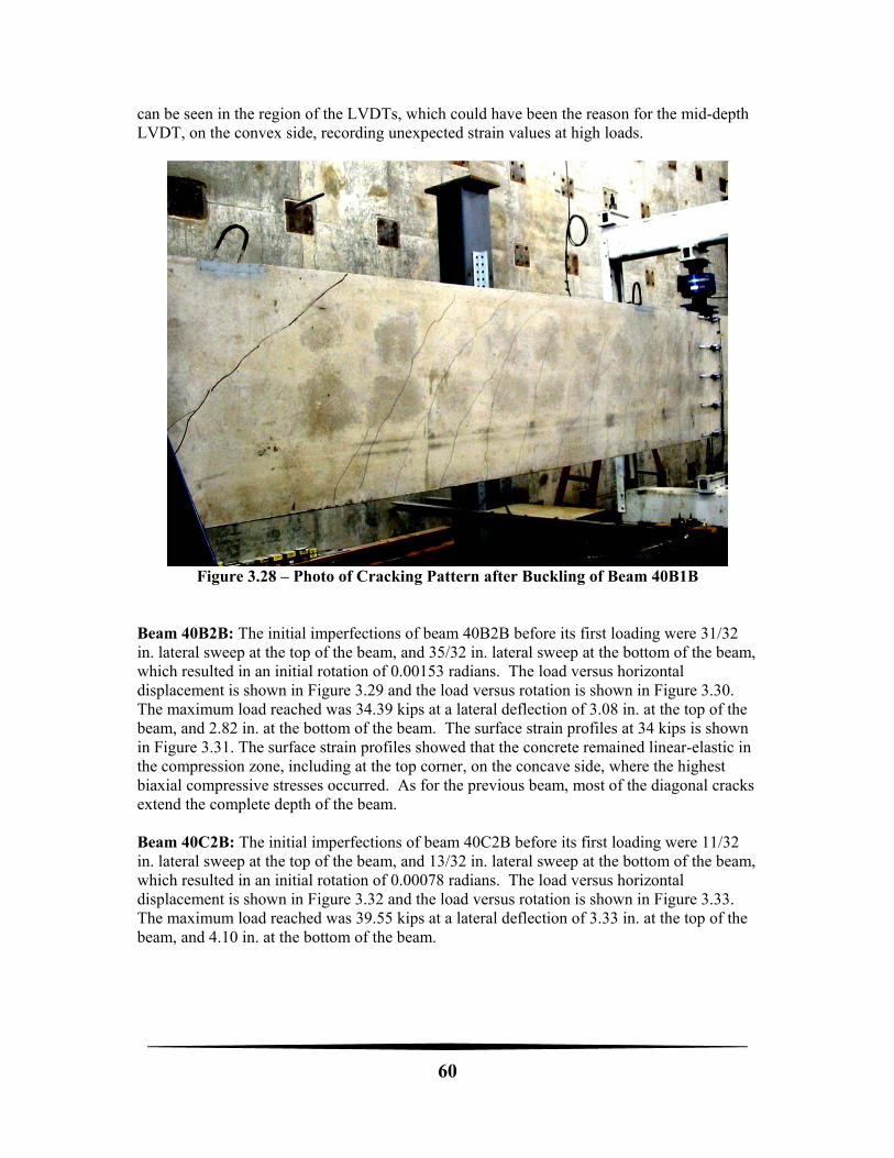
60

can be seen in the region of the LVDTs, which could have been the reason for the mid-depth LVDT, on the convex side, recording unexpected strain values at high loads.

Figure 3.28 – Photo of Cracking Pattern after Buckling of Beam 40B1B

Beam 40B2B: The initial imperfections of beam 40B2B before its first loading were 31/32 in. lateral sweep at the top of the beam, and 35/32 in. lateral sweep at the bottom of the beam, which resulted in an initial rotation of 0.00153 radians. The load versus horizontal displacement is shown in Figure 3.29 and the load versus rotation is shown in Figure 3.30. The maximum load reached was 34.39 kips at a lateral deflection of 3.08 in. at the top of the beam, and 2.82 in. at the bottom of the beam. The surface strain profiles at 34 kips is shown in Figure 3.31. The surface strain profiles showed that the concrete remained linear-elastic in the compression zone, including at the top corner, on the concave side, where the highest biaxial compressive stresses occurred. As for the previous beam, most of the diagonal cracks extend the complete depth of the beam. Beam 40C2B: The initial imperfections of beam 40C2B before its first loading were 11/32 in. lateral sweep at the top of the beam, and 13/32 in. lateral sweep at the bottom of the beam, which resulted in an initial rotation of 0.00078 radians. The load versus horizontal displacement is shown in Figure 3.32 and the load versus rotation is shown in Figure 3.33. The maximum load reached was 39.55 kips at a lateral deflection of 3.33 in. at the top of the beam, and 4.10 in. at the bottom of the beam.

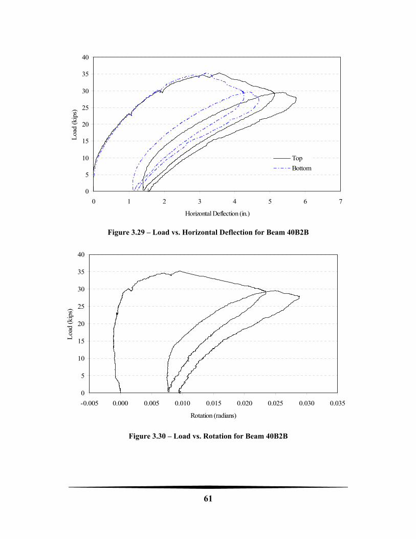
61

Figure 3.29 – Load vs. Horizontal Deflection for Beam 40B2B

Figure 3.30 – Load vs. Rotation for Beam 40B2B

0

5

10

15

20

25

30

35

40

0 1 2 3 4 5 6 7

Horizontal Deflection (in.)

Loa

d (k

ips)

Top

Bottom

0

5

10

15

20

25

30

35

40

-0.005 0.000 0.005 0.010 0.015 0.020 0.025 0.030 0.035

Rotation (radians)

Loa

d (k

ips)

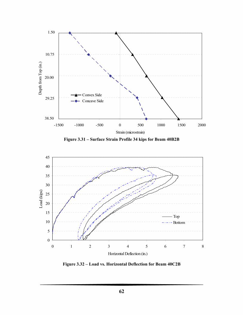
62

Figure 3.31 – Surface Strain Profile 34 kips for Beam 40B2B

Figure 3.32 – Load vs. Horizontal Deflection for Beam 40C2B

-1500 -1000 -500 0 500 1000 1500 2000

Strain (microstrain)

Dep

th f

rom

Top

(in

.)

Convex Side

Concave Side

1.50

10.75

38.50

29.25

20.00

0

5

10

15

20

25

30

35

40

45

0 1 2 3 4 5 6 7 8

Horizontal Deflection (in.)

Loa

d (k

ips)

Top

Bottom

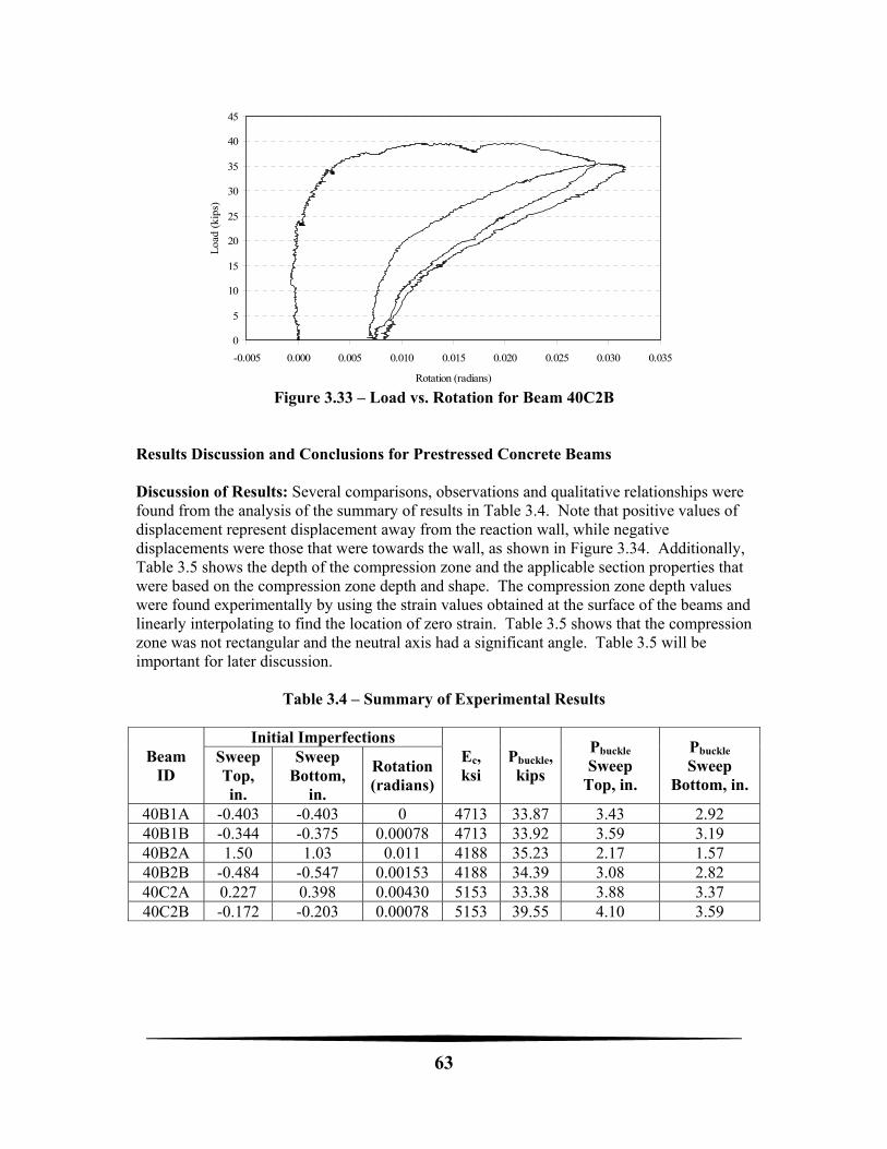
63

Figure 3.33 – Load vs. Rotation for Beam 40C2B

Results Discussion and Conclusions for Prestressed Concrete Beams Discussion of Results: Several comparisons, observations and qualitative relationships were found from the analysis of the summary of results in Table 3.4. Note that positive values of displacement represent displacement away from the reaction wall, while negative displacements were those that were towards the wall, as shown in Figure 3.34. Additionally, Table 3.5 shows the depth of the compression zone and the applicable section properties that were based on the compression zone depth and shape. The compression zone depth values were found experimentally by using the strain values obtained at the surface of the beams and linearly interpolating to find the location of zero strain. Table 3.5 shows that the compression zone was not rectangular and the neutral axis had a significant angle. Table 3.5 will be important for later discussion.

Table 3.4 – Summary of Experimental Results

Beam ID

Initial Imperfections Ec, ksi

Pbuckle,kips

Pbuckle Sweep

Top, in.

Pbuckle Sweep

Bottom, in.

Sweep Top, in.

Sweep Bottom,

in.

Rotation(radians)

40B1A -0.403 -0.403 0 4713 33.87 3.43 2.92 40B1B -0.344 -0.375 0.00078 4713 33.92 3.59 3.19 40B2A 1.50 1.03 0.011 4188 35.23 2.17 1.57 40B2B -0.484 -0.547 0.00153 4188 34.39 3.08 2.82 40C2A 0.227 0.398 0.00430 5153 33.38 3.88 3.37 40C2B -0.172 -0.203 0.00078 5153 39.55 4.10 3.59

0

5

10

15

20

25

30

35

40

45

-0.005 0.000 0.005 0.010 0.015 0.020 0.025 0.030 0.035

Rotation (radians)

Loa

d (k

ips)

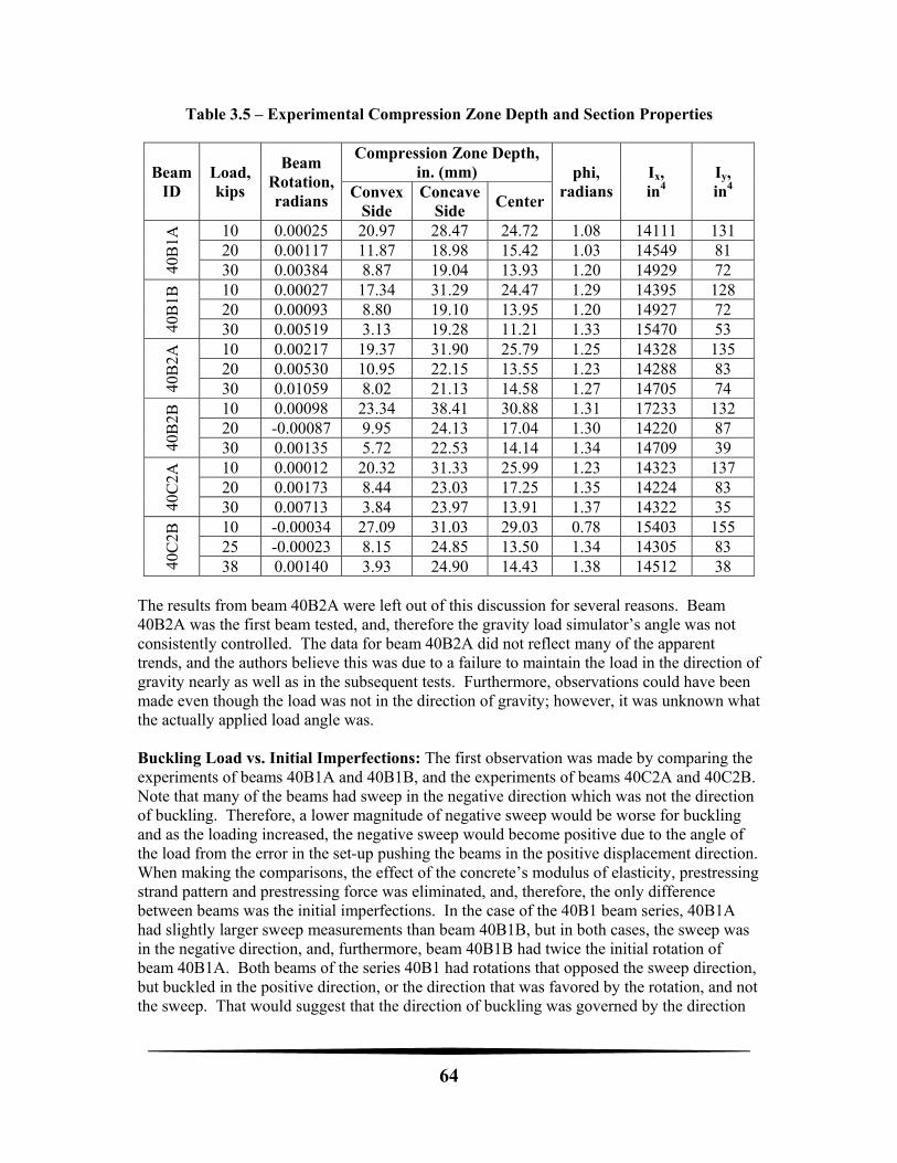
64

Table 3.5 – Experimental Compression Zone Depth and Section Properties

Beam ID

Load, kips

Beam Rotation, radians

Compression Zone Depth, in. (mm) phi,

radiansIx, in4

Iy, in4 Convex

Side Concave

Side Center

40B

1A

10 0.00025 20.97 28.47 24.72 1.08 14111 131 20 0.00117 11.87 18.98 15.42 1.03 14549 81 30 0.00384 8.87 19.04 13.93 1.20 14929 72

40B

1B

10 0.00027 17.34 31.29 24.47 1.29 14395 128 20 0.00093 8.80 19.10 13.95 1.20 14927 72 30 0.00519 3.13 19.28 11.21 1.33 15470 53

40B

2A

10 0.00217 19.37 31.90 25.79 1.25 14328 135 20 0.00530 10.95 22.15 13.55 1.23 14288 83 30 0.01059 8.02 21.13 14.58 1.27 14705 74

40B

2B

10 0.00098 23.34 38.41 30.88 1.31 17233 132 20 -0.00087 9.95 24.13 17.04 1.30 14220 87 30 0.00135 5.72 22.53 14.14 1.34 14709 39

40C

2A

10 0.00012 20.32 31.33 25.99 1.23 14323 137 20 0.00173 8.44 23.03 17.25 1.35 14224 83 30 0.00713 3.84 23.97 13.91 1.37 14322 35

40C

2B

10 -0.00034 27.09 31.03 29.03 0.78 15403 155 25 -0.00023 8.15 24.85 13.50 1.34 14305 83 38 0.00140 3.93 24.90 14.43 1.38 14512 38

The results from beam 40B2A were left out of this discussion for several reasons. Beam 40B2A was the first beam tested, and, therefore the gravity load simulator’s angle was not consistently controlled. The data for beam 40B2A did not reflect many of the apparent trends, and the authors believe this was due to a failure to maintain the load in the direction of gravity nearly as well as in the subsequent tests. Furthermore, observations could have been made even though the load was not in the direction of gravity; however, it was unknown what the actually applied load angle was. Buckling Load vs. Initial Imperfections: The first observation was made by comparing the experiments of beams 40B1A and 40B1B, and the experiments of beams 40C2A and 40C2B. Note that many of the beams had sweep in the negative direction which was not the direction of buckling. Therefore, a lower magnitude of negative sweep would be worse for buckling and as the loading increased, the negative sweep would become positive due to the angle of the load from the error in the set-up pushing the beams in the positive displacement direction. When making the comparisons, the effect of the concrete’s modulus of elasticity, prestressing strand pattern and prestressing force was eliminated, and, therefore, the only difference between beams was the initial imperfections. In the case of the 40B1 beam series, 40B1A had slightly larger sweep measurements than beam 40B1B, but in both cases, the sweep was in the negative direction, and, furthermore, beam 40B1B had twice the initial rotation of beam 40B1A. Both beams of the series 40B1 had rotations that opposed the sweep direction, but buckled in the positive direction, or the direction that was favored by the rotation, and not the sweep. That would suggest that the direction of buckling was governed by the direction

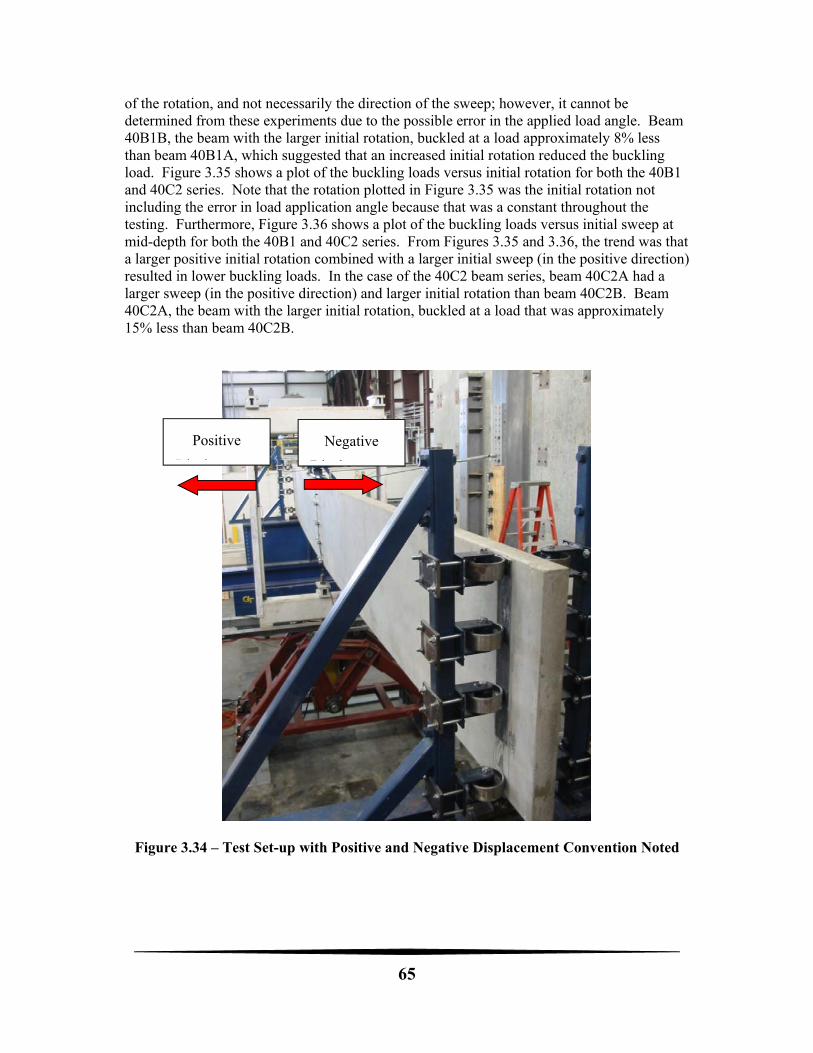
65

of the rotation, and not necessarily the direction of the sweep; however, it cannot be determined from these experiments due to the possible error in the applied load angle. Beam 40B1B, the beam with the larger initial rotation, buckled at a load approximately 8% less than beam 40B1A, which suggested that an increased initial rotation reduced the buckling load. Figure 3.35 shows a plot of the buckling loads versus initial rotation for both the 40B1 and 40C2 series. Note that the rotation plotted in Figure 3.35 was the initial rotation not including the error in load application angle because that was a constant throughout the testing. Furthermore, Figure 3.36 shows a plot of the buckling loads versus initial sweep at mid-depth for both the 40B1 and 40C2 series. From Figures 3.35 and 3.36, the trend was that a larger positive initial rotation combined with a larger initial sweep (in the positive direction) resulted in lower buckling loads. In the case of the 40C2 beam series, beam 40C2A had a larger sweep (in the positive direction) and larger initial rotation than beam 40C2B. Beam 40C2A, the beam with the larger initial rotation, buckled at a load that was approximately 15% less than beam 40C2B.

Figure 3.34 – Test Set-up with Positive and Negative Displacement Convention Noted

Negative

Di l

Positive

Di l

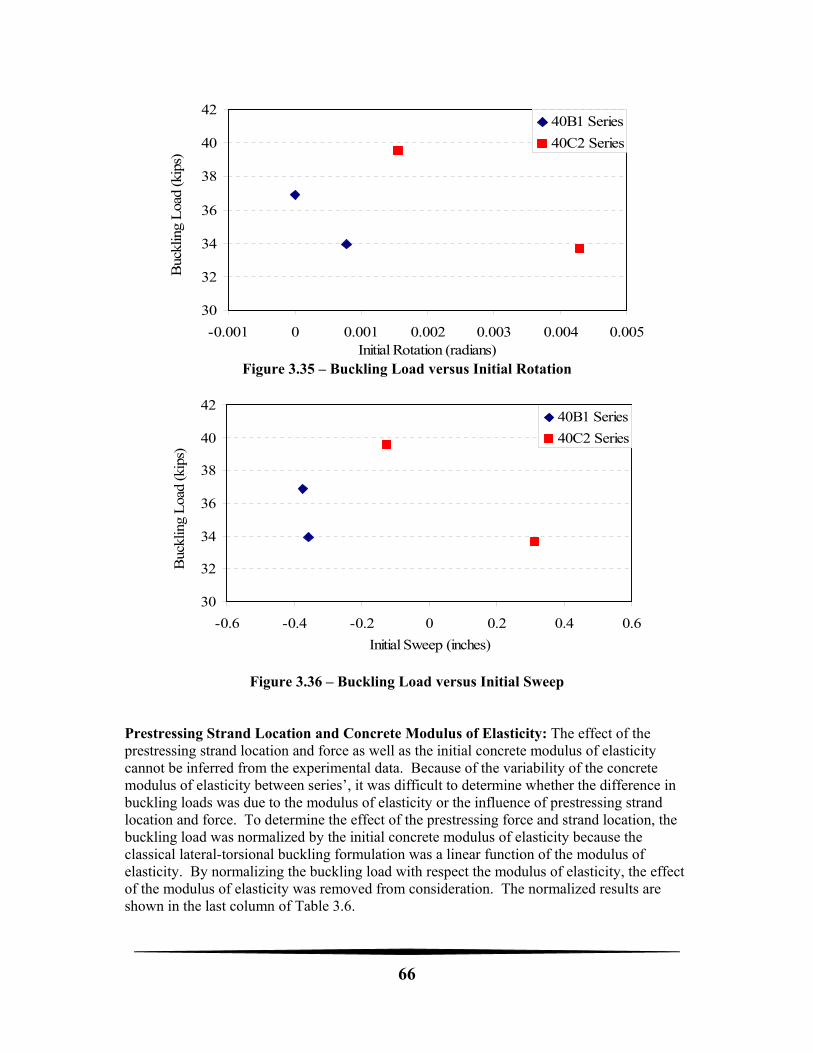
66

Figure 3.35 – Buckling Load versus Initial Rotation

Figure 3.36 – Buckling Load versus Initial Sweep Prestressing Strand Location and Concrete Modulus of Elasticity: The effect of the prestressing strand location and force as well as the initial concrete modulus of elasticity cannot be inferred from the experimental data. Because of the variability of the concrete modulus of elasticity between series’, it was difficult to determine whether the difference in buckling loads was due to the modulus of elasticity or the influence of prestressing strand location and force. To determine the effect of the prestressing force and strand location, the buckling load was normalized by the initial concrete modulus of elasticity because the classical lateral-torsional buckling formulation was a linear function of the modulus of elasticity. By normalizing the buckling load with respect the modulus of elasticity, the effect of the modulus of elasticity was removed from consideration. The normalized results are shown in the last column of Table 3.6.

30

32

34

36

38

40

42

-0.001 0 0.001 0.002 0.003 0.004 0.005Initial Rotation (radians)

Buc

klin

g L

oad

(kip

s)

40B1 Series

40C2 Series

30

32

34

36

38

40

42

-0.6 -0.4 -0.2 0 0.2 0.4 0.6

Initial Sweep (inches)

Buc

klin

g L

oad

(kip

s)

40B1 Series

40C2 Series

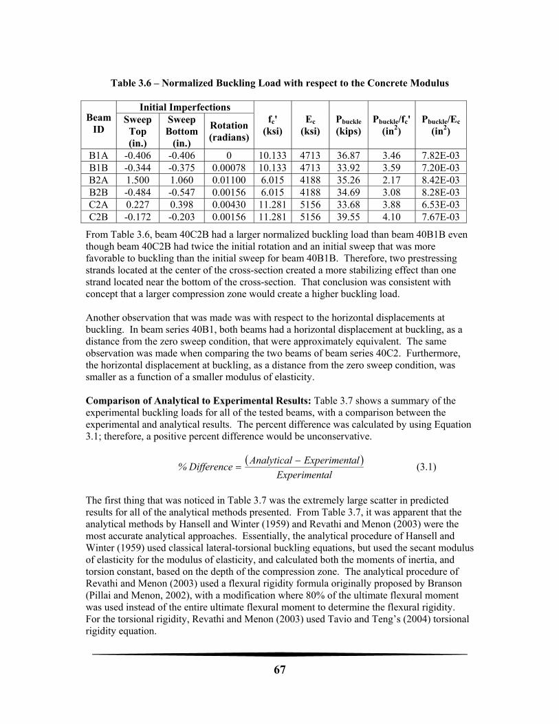
67

Table 3.6 – Normalized Buckling Load with respect to the Concrete Modulus

Beam ID

Initial Imperfections fc'

(ksi) Ec

(ksi) Pbuckle

(kips) Pbuckle/fc'

(in2) Pbuckle/Ec

(in2) Sweep Top (in.)

Sweep Bottom

(in.)

Rotation(radians)

B1A -0.406 -0.406 0 10.133 4713 36.87 3.46 7.82E-03 B1B -0.344 -0.375 0.00078 10.133 4713 33.92 3.59 7.20E-03 B2A 1.500 1.060 0.01100 6.015 4188 35.26 2.17 8.42E-03 B2B -0.484 -0.547 0.00156 6.015 4188 34.69 3.08 8.28E-03 C2A 0.227 0.398 0.00430 11.281 5156 33.68 3.88 6.53E-03 C2B -0.172 -0.203 0.00156 11.281 5156 39.55 4.10 7.67E-03

From Table 3.6, beam 40C2B had a larger normalized buckling load than beam 40B1B even though beam 40C2B had twice the initial rotation and an initial sweep that was more favorable to buckling than the initial sweep for beam 40B1B. Therefore, two prestressing strands located at the center of the cross-section created a more stabilizing effect than one strand located near the bottom of the cross-section. That conclusion was consistent with concept that a larger compression zone would create a higher buckling load. Another observation that was made was with respect to the horizontal displacements at buckling. In beam series 40B1, both beams had a horizontal displacement at buckling, as a distance from the zero sweep condition, that were approximately equivalent. The same observation was made when comparing the two beams of beam series 40C2. Furthermore, the horizontal displacement at buckling, as a distance from the zero sweep condition, was smaller as a function of a smaller modulus of elasticity. Comparison of Analytical to Experimental Results: Table 3.7 shows a summary of the experimental buckling loads for all of the tested beams, with a comparison between the experimental and analytical results. The percent difference was calculated by using Equation 3.1; therefore, a positive percent difference would be unconservative.

alExperiment

alExperimentAnalyticalDifference%

(3.1)

The first thing that was noticed in Table 3.7 was the extremely large scatter in predicted results for all of the analytical methods presented. From Table 3.7, it was apparent that the analytical methods by Hansell and Winter (1959) and Revathi and Menon (2003) were the most accurate analytical approaches. Essentially, the analytical procedure of Hansell and Winter (1959) used classical lateral-torsional buckling equations, but used the secant modulus of elasticity for the modulus of elasticity, and calculated both the moments of inertia, and torsion constant, based on the depth of the compression zone. The analytical procedure of Revathi and Menon (2003) used a flexural rigidity formula originally proposed by Branson (Pillai and Menon, 2002), with a modification where 80% of the ultimate flexural moment was used instead of the entire ultimate flexural moment to determine the flexural rigidity. For the torsional rigidity, Revathi and Menon (2003) used Tavio and Teng’s (2004) torsional rigidity equation.

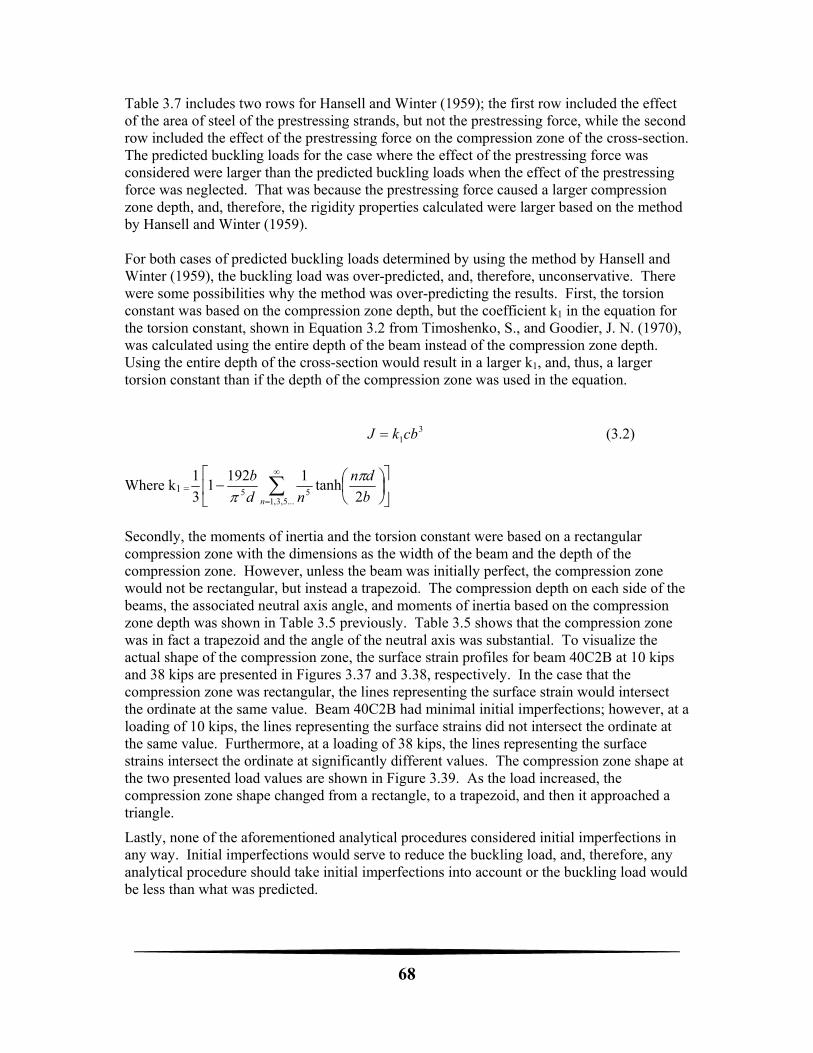
68

Table 3.7 includes two rows for Hansell and Winter (1959); the first row included the effect of the area of steel of the prestressing strands, but not the prestressing force, while the second row included the effect of the prestressing force on the compression zone of the cross-section. The predicted buckling loads for the case where the effect of the prestressing force was considered were larger than the predicted buckling loads when the effect of the prestressing force was neglected. That was because the prestressing force caused a larger compression zone depth, and, therefore, the rigidity properties calculated were larger based on the method by Hansell and Winter (1959). For both cases of predicted buckling loads determined by using the method by Hansell and Winter (1959), the buckling load was over-predicted, and, therefore, unconservative. There were some possibilities why the method was over-predicting the results. First, the torsion constant was based on the compression zone depth, but the coefficient k1 in the equation for the torsion constant, shown in Equation 3.2 from Timoshenko, S., and Goodier, J. N. (1970), was calculated using the entire depth of the beam instead of the compression zone depth. Using the entire depth of the cross-section would result in a larger k1, and, thus, a larger torsion constant than if the depth of the compression zone was used in the equation. 3

1cbkJ (3.2)

Where k1 =

...5,3,155 2

tanh1192

13

1

n b

dn

nd

b

Secondly, the moments of inertia and the torsion constant were based on a rectangular compression zone with the dimensions as the width of the beam and the depth of the compression zone. However, unless the beam was initially perfect, the compression zone would not be rectangular, but instead a trapezoid. The compression depth on each side of the beams, the associated neutral axis angle, and moments of inertia based on the compression zone depth was shown in Table 3.5 previously. Table 3.5 shows that the compression zone was in fact a trapezoid and the angle of the neutral axis was substantial. To visualize the actual shape of the compression zone, the surface strain profiles for beam 40C2B at 10 kips and 38 kips are presented in Figures 3.37 and 3.38, respectively. In the case that the compression zone was rectangular, the lines representing the surface strain would intersect the ordinate at the same value. Beam 40C2B had minimal initial imperfections; however, at a loading of 10 kips, the lines representing the surface strains did not intersect the ordinate at the same value. Furthermore, at a loading of 38 kips, the lines representing the surface strains intersect the ordinate at significantly different values. The compression zone shape at the two presented load values are shown in Figure 3.39. As the load increased, the compression zone shape changed from a rectangle, to a trapezoid, and then it approached a triangle.

Lastly, none of the aforementioned analytical procedures considered initial imperfections in any way. Initial imperfections would serve to reduce the buckling load, and, therefore, any analytical procedure should take initial imperfections into account or the buckling load would be less than what was predicted.

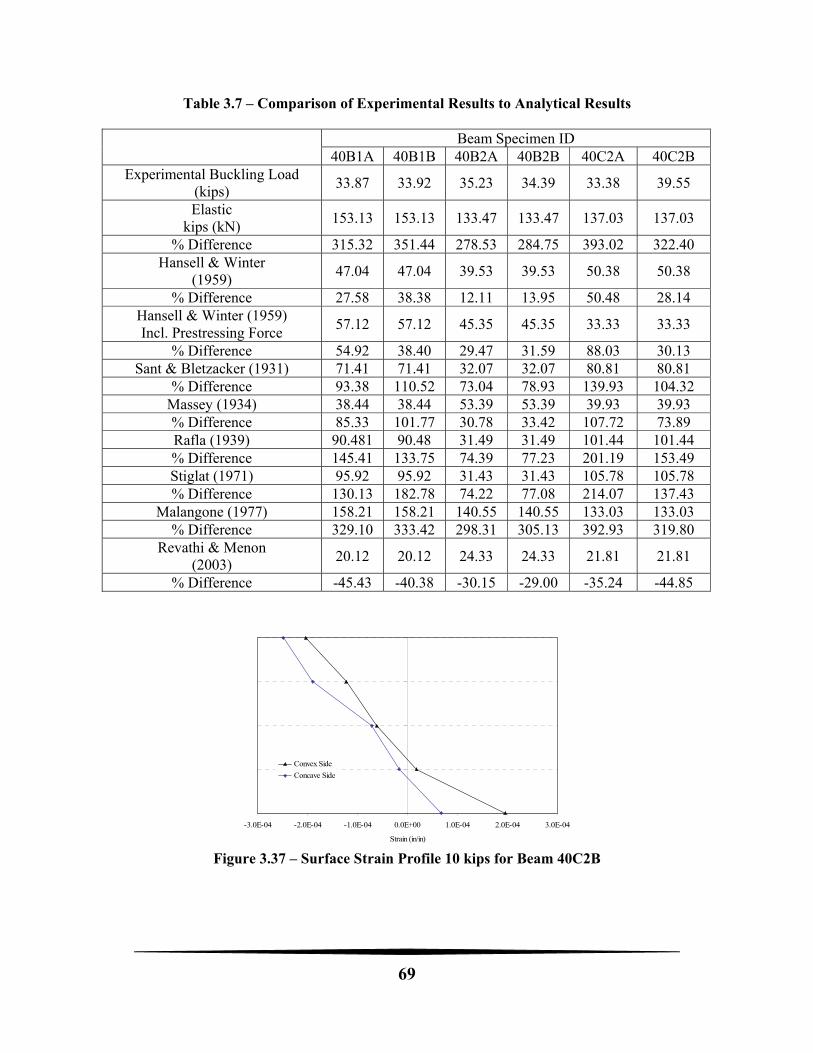
69

Table 3.7 – Comparison of Experimental Results to Analytical Results

Beam Specimen ID 40B1A 40B1B 40B2A 40B2B 40C2A 40C2B

Experimental Buckling Load (kips)

33.87 33.92 35.23 34.39 33.38 39.55

Elastic kips (kN)

153.13 153.13 133.47 133.47 137.03 137.03

% Difference 315.32 351.44 278.53 284.75 393.02 322.40 Hansell & Winter

(1959) 47.04 47.04 39.53 39.53 50.38 50.38

% Difference 27.58 38.38 12.11 13.95 50.48 28.14 Hansell & Winter (1959) Incl. Prestressing Force

57.12 57.12 45.35 45.35 33.33 33.33

% Difference 54.92 38.40 29.47 31.59 88.03 30.13 Sant & Bletzacker (1931) 71.41 71.41 32.07 32.07 80.81 80.81

% Difference 93.38 110.52 73.04 78.93 139.93 104.32 Massey (1934) 38.44 38.44 53.39 53.39 39.93 39.93 % Difference 85.33 101.77 30.78 33.42 107.72 73.89 Rafla (1939) 90.481 90.48 31.49 31.49 101.44 101.44 % Difference 145.41 133.75 74.39 77.23 201.19 153.49 Stiglat (1971) 95.92 95.92 31.43 31.43 105.78 105.78 % Difference 130.13 182.78 74.22 77.08 214.07 137.43

Malangone (1977) 158.21 158.21 140.55 140.55 133.03 133.03% Difference 329.10 333.42 298.31 305.13 392.93 319.80

Revathi & Menon (2003)

20.12 20.12 24.33 24.33 21.81 21.81

% Difference -45.43 -40.38 -30.15 -29.00 -35.24 -44.85

Figure 3.37 – Surface Strain Profile 10 kips for Beam 40C2B

-3.0E-04 -2.0E-04 -1.0E-04 0.0E+00 1.0E-04 2.0E-04 3.0E-04

Strain (in/in)

Convex Side

Concave Side

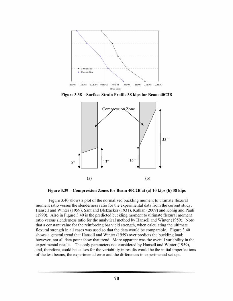
70

Figure 3.38 – Surface Strain Profile 38 kips for Beam 40C2B

Figure 3.39 – Compression Zones for Beam 40C2B at (a) 10 kips (b) 38 kips

Figure 3.40 shows a plot of the normalized buckling moment to ultimate flexural moment ratio versus the slenderness ratio for the experimental data from the current study, Hansell and Winter (1959), Sant and Bletzacker (1931), Kalkan (2009) and König and Pauli (1990). Also in Figure 3.40 is the predicted buckling moment to ultimate flexural moment ratio versus slenderness ratio for the analytical method by Hansell and Winter (1959). Note that a constant value for the reinforcing bar yield strength, when calculating the ultimate flexural strength in all cases was used so that the data would be comparable. Figure 3.40 shows a general trend that Hansell and Winter (1959) over predicts the buckling load; however, not all data point show that trend. More apparent was the overall variability in the experimental results. The only parameters not considered by Hansell and Winter (1959), and, therefore, could be causes for the variability in results would be the initial imperfections of the test beams, the experimental error and the differences in experimental set-ups.

-1.5E-03 -1.0E-03 -5.0E-04 0.0E+00 5.0E-04 1.0E-03 1.5E-03 2.0E-03 2.5E-03

Strain (in/in)

Convex Side

Concave Side

(a) (b)

9” 13” 15”

33”

Compression Zone

71

The analytical procedure by Revathi and Menon (2003) under-predicted the experimental buckling loads, but by a non-negligible amount. That would be good from a safety standpoint, but would not be good for design economy or from the academic standpoint of understanding the actual behavior. Furthermore, the analytical procedure by Revathi and Menon (2003) did not consider initial imperfections; therefore, any modification to their method that included the effect of initial imperfections would decrease the accuracy of the prediction. A similar plot to the one in Figure 3.40 is shown in Figure 3.41 except that the experimental data was compared with the analytical procedure by Revathi and Menon (2003). Figure 3.41 shows that all the experimental results were higher than what was predicted by Revathi and Menon (2003), and, therefore, does not represent the actual behavior and would potentially be too conservative.

Figure 3.40 – Buckling Moment to Ultimate Flexural Moment Ratio versus Slenderness

Ratio for Test Data Compared with Hansell and Winter (1959) Analysis

Figure 3.41 – Buckling Moment to Ultimate Flexural Moment Ratio versus Slenderness

Ratio for Test Data Compared with Revathi and Menon (2003) Analysis

0

0.2

0.4

0.6

0.8

1

1.2

0 200 400 600 800 1000 1200 1400 1600Slenderness Ratio Ld/b2

Mb/

Mul

t

Hansell & Winter (1959) Pred.

Hansell & Winter (1959) Exp.

Current Study Exp.

Kalkan (2009) Exp.

Sant & Bletzacker (1961) Exp.

0

0.2

0.4

0.6

0.8

1

1.2

0 200 400 600 800 1000 1200 1400 1600Slenderness Ratio Ld/b2

Mb/

Mul

t

Revathi & Menon (2006) Pred.Hansell & Winter (1959) Exp.

Current Study Exp.Kalkan (2009) Exp.

Sant & Bletzacker (1961) Exp.

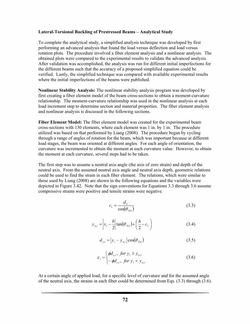
72

Lateral-Torsional Buckling of Prestressed Beams – Analytical Study To complete the analytical study, a simplified analysis technique was developed by first performing an advanced analysis that found the load versus deflection and load versus rotation plots. The procedure involved a fiber element analysis and a nonlinear analysis. The obtained plots were compared to the experimental results to validate the advanced analysis. After validation was accomplished, the analysis was run for different initial imperfections for the different beams such that the accuracy of a proposed simplified equation could be verified. Lastly, the simplified technique was compared with available experimental results where the initial imperfections of the beams were published. Nonlinear Stability Analysis: The nonlinear stability analysis program was developed by first creating a fiber element model of the beam cross-sections to obtain a moment-curvature relationship. The moment-curvature relationship was used in the nonlinear analysis at each load increment step to determine section and material properties. The fiber element analysis and nonlinear analysis is discussed in the following sections. Fiber Element Model: The fiber element model was created for the experimental beam cross-sections with 130 elements, where each element was 1 in. by 1 in. The procedure utilized was based on that performed by Liang (2008). The procedure began by cycling through a range of angles of rotation for the beam, which was important because at different load stages, the beam was oriented at different angles. For each angle of orientation, the curvature was incremented to obtain the moment at each curvature value. However, to obtain the moment at each curvature, several steps had to be taken. The first step was to assume a neutral axis angle (the axis of zero strain) and depth of the neutral axis. From the assumed neutral axis angle and neutral axis depth, geometric relations could be used to find the strain in each fiber element. The relations, which were similar to those used by Liang (2008) are shown in the following equations and the variables were depicted in Figure 3.42. Note that the sign conventions for Equations 3.3 through 3.6 assume compressive strains were positive and tensile strains were negative.

NA

ndc

cos1 (3.3)

1, 2

tan2

chb

xy NAiin (3.4)

NAiniie yyd cos,, (3.5)

iniie

iniie

i yyford

yyford

,,

,,

,

,

(3.6)

At a certain angle of applied load, for a specific level of curvature and for the assumed angle of the neutral axis, the strains in each fiber could be determined from Eqs. (3.3) through (3.6).

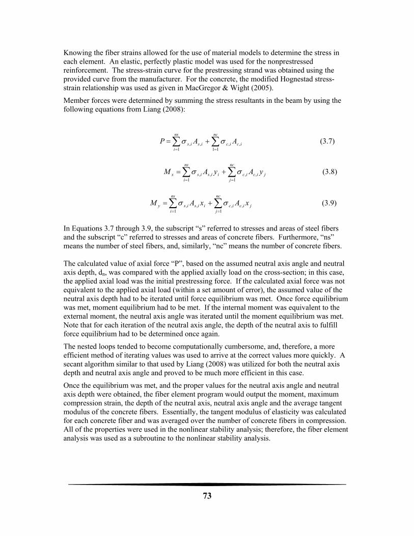
73

Knowing the fiber strains allowed for the use of material models to determine the stress in each element. An elastic, perfectly plastic model was used for the nonprestressed reinforcement. The stress-strain curve for the prestressing strand was obtained using the provided curve from the manufacturer. For the concrete, the modified Hognestad stress-strain relationship was used as given in MacGregor & Wight (2005).

Member forces were determined by summing the stress resultants in the beam by using the following equations from Liang (2008):

nc

icic

ns

iisis AAP

11,,

1,, (3.7)

nc

jjicic

ns

iiisisx yAyAM

1,,

1,,

(3.8)

nc

jjicic

ns

iiisisy xAxAM

1,,

1,, (3.9)

In Equations 3.7 through 3.9, the subscript “s” referred to stresses and areas of steel fibers and the subscript “c” referred to stresses and areas of concrete fibers. Furthermore, “ns” means the number of steel fibers, and, similarly, “nc” means the number of concrete fibers. The calculated value of axial force “P”, based on the assumed neutral axis angle and neutral axis depth, dn, was compared with the applied axially load on the cross-section; in this case, the applied axial load was the initial prestressing force. If the calculated axial force was not equivalent to the applied axial load (within a set amount of error), the assumed value of the neutral axis depth had to be iterated until force equilibrium was met. Once force equilibrium was met, moment equilibrium had to be met. If the internal moment was equivalent to the external moment, the neutral axis angle was iterated until the moment equilibrium was met. Note that for each iteration of the neutral axis angle, the depth of the neutral axis to fulfill force equilibrium had to be determined once again.

The nested loops tended to become computationally cumbersome, and, therefore, a more efficient method of iterating values was used to arrive at the correct values more quickly. A secant algorithm similar to that used by Liang (2008) was utilized for both the neutral axis depth and neutral axis angle and proved to be much more efficient in this case.

Once the equilibrium was met, and the proper values for the neutral axis angle and neutral axis depth were obtained, the fiber element program would output the moment, maximum compression strain, the depth of the neutral axis, neutral axis angle and the average tangent modulus of the concrete fibers. Essentially, the tangent modulus of elasticity was calculated for each concrete fiber and was averaged over the number of concrete fibers in compression. All of the properties were used in the nonlinear stability analysis; therefore, the fiber element analysis was used as a subroutine to the nonlinear stability analysis.

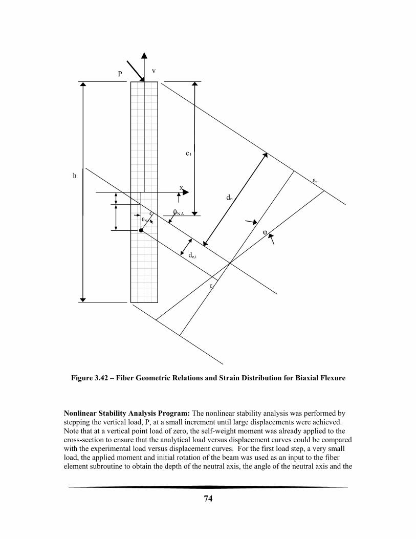
74

Figure 3.42 – Fiber Geometric Relations and Strain Distribution for Biaxial Flexure Nonlinear Stability Analysis Program: The nonlinear stability analysis was performed by stepping the vertical load, P, at a small increment until large displacements were achieved. Note that at a vertical point load of zero, the self-weight moment was already applied to the cross-section to ensure that the analytical load versus displacement curves could be compared with the experimental load versus displacement curves. For the first load step, a very small load, the applied moment and initial rotation of the beam was used as an input to the fiber element subroutine to obtain the depth of the neutral axis, the angle of the neutral axis and the

P

θNAθNA

h

φ

εt

εi

x

y

c1

dn

de,i

75

average tangent modulus of the compression zone. The depth of the neutral axis and angle of the neutral axis was used to calculate the moments of inertia based on the shape of the compression zone and the transformed area of the steel. The torsion constant was based on a rectangular compression zone and was calculated by using Equation 3.2. The critical buckling moment was calculated by using the following equation:

JGIEL

CM ybb tantan

(3.10)

The value for Cb was calculated using the following equation (Trahair, 1993):

JG

IE

L

aC

yb

tan

tan74.1135.1 (3.11)

The value of 1.35 in Eq. (3.11) was used to take into account the moment gradient for the case of a point load on a simply-supported beam. The second portion of the equation was used to take into account the effect of the load height on the stability of the beam. Once the value of the buckling moment for the specific load increment was determined, Eqs. (3.12) through (3.15) from Chen & Lui (1987) could be used to determine the horizontal displacement and the rotation of the beam for the specific load increment.

L

z

MM

MMu

b

b sin

1 00

0

(3.12)

L

z

MM

MM

b

b sin

1 00

0

(3.13)

L

zsinu 00

(3.14)

L

zsin00

( 3.15)

Note that the use of Eqs. (3.12) through (3.15) assumed a uniform moment applied to the beam, and that the initial sweep and rotation followed a sine curve. There was no closed-form solution available for the case of a point load applied to an imperfect beam, and numerical techniques would have to be used to solve the associated differential equations. Although the tested beams in this study had a concentrated load applied to them, Equations 3.12 through 3.15 were used because the factor Cb would account for the difference in buckling load, and, therefore, an accurate prediction of the buckling load would still be obtained.

76

Once the horizontal displacement and rotation was determined for a load increment, the process was repeated for the next load increment. Essentially, for every load increment, there would be a different value of the rotation; therefore, the fiber element subroutine was used for every load increment. Furthermore, when the stresses became high enough, the modulus of elasticity was less than the initial modulus of elasticity, and, therefore, the value of Mb in Equations 3.12 and 3.13 would become smaller. The process can be best summarized in the flowchart shown below in Figure 3.43. Nonlinear Stability Analysis Results: The nonlinear stability analysis was run for all of the beams except for 40B2A because that was the beam where the angle of the applied load was unknown. For all of the other test beams, there was a 0.008727 radian error in the applied vertical load; however, it was a known quantity that was taken into account in the analysis. Method to Account for Error in Load Angle: The error in the load angle was taken into account in the nonlinear stability analysis by altering the initial sweep and initial rotation terms in Equations 3.12 and 3.13. Normally, the analysis would involve using a constant value for the initial imperfections in Equations 3.4.10 and 3.13. But instead, to account for the error, the initial imperfections used in Equations 3.12 and 3.13 were changed for each load increment. In the case of the initial horizontal sweep, at each load increment, the initial horizontal sweep was added to the horizontal displacement due to a horizontal load that was a function of the total applied load and the sine of the error angle as shown in Equation 3.16. errorP sin* 00 (3.16)

The initial rotation was altered in a similar fashion as shown in Equation 3.17. errorP sin* 00 (3.17)

Nonlinear Analysis Results vs. Experimental Results: The results of the nonlinear analysis are depicted in Figures 3.44 to 3.53 for beams 40B1A, 40B1B, 40B2B, 40C2A and 40C2B. For each of the beams, both the load versus horizontal displacement and load versus rotation are shown. The initial imperfections used in the analysis were those measured prior to each of the experiments. It was apparent from Figures 3.44 through 3.53 that the nonlinear analysis matched the experimental load versus horizontal displacement and load versus rotation curves well. Furthermore, the nonlinear analysis predicted the maximum load well. The differences in predicted maximum load can be attributed to error in measuring the initial imperfections and the possibility of “settlement” in components of the test set-up, such as the end supports, once loading began. The possibility of error in measuring the initial imperfections was a strong possibility because the nonlinear analysis results varied significantly with varying initial imperfections with all other parameters equivalent. The other discrepancy that was noticed in the comparison of the load versus horizontal displacement curves for the nonlinear analysis and the experimental curve was the shape of the curve. There was a significant gap between the two curves that begins in the range of 10 kips and reduces as the maximum load was approached. The difference between the curves was most probably due to two factors. The first factor was that the closed form solution for the horizontal displacement was based on an applied constant moment and not a midspan

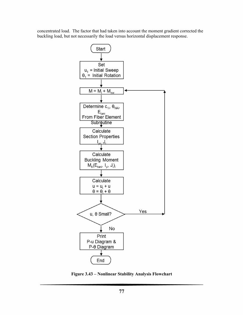
77

concentrated load. The factor that had taken into account the moment gradient corrected the buckling load, but not necessarily the load versus horizontal displacement response.

Figure 3.43 – Nonlinear Stability Analysis Flowchart

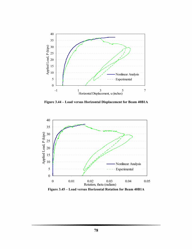
78

Figure 3.44 – Load versus Horizontal Displacement for Beam 40B1A

Figure 3.45 – Load versus Horizontal Rotation for Beam 40B1A

0

5

10

15

20

25

30

35

40

-1 1 3 5 7Horizontal Displacement, u (inches)

App

lied

Loa

d, P

(ki

ps)

Nonlinear Analysis

Experimental

0

5

10

15

20

25

30

35

40

0 0.01 0.02 0.03 0.04 0.05Rotation, theta (radians)

App

lied

Loa

d, P

(ki

ps)

Nonlinear Analysis

Experimental

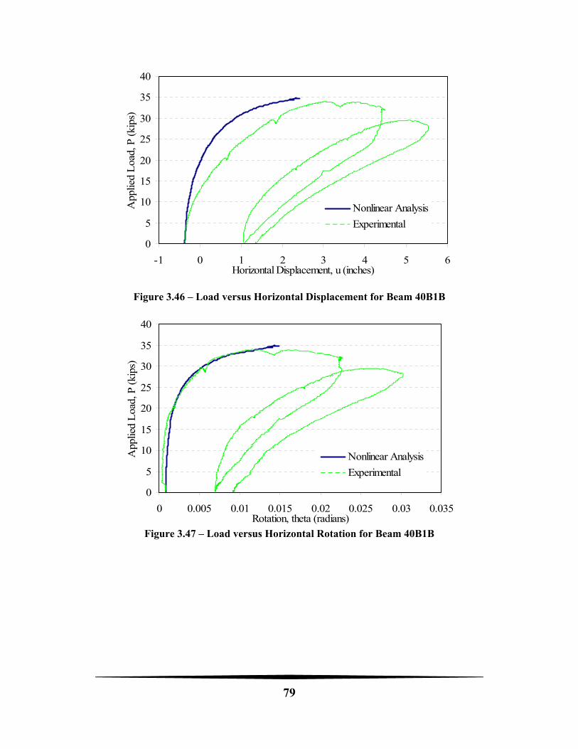
79

Figure 3.46 – Load versus Horizontal Displacement for Beam 40B1B

Figure 3.47 – Load versus Horizontal Rotation for Beam 40B1B

0

5

10

15

20

25

30

35

40

-1 0 1 2 3 4 5 6Horizontal Displacement, u (inches)

App

lied

Loa

d, P

(ki

ps)

Nonlinear Analysis

Experimental

0

5

10

15

20

25

30

35

40

0 0.005 0.01 0.015 0.02 0.025 0.03 0.035Rotation, theta (radians)

App

lied

Loa

d, P

(ki

ps)

Nonlinear Analysis

Experimental

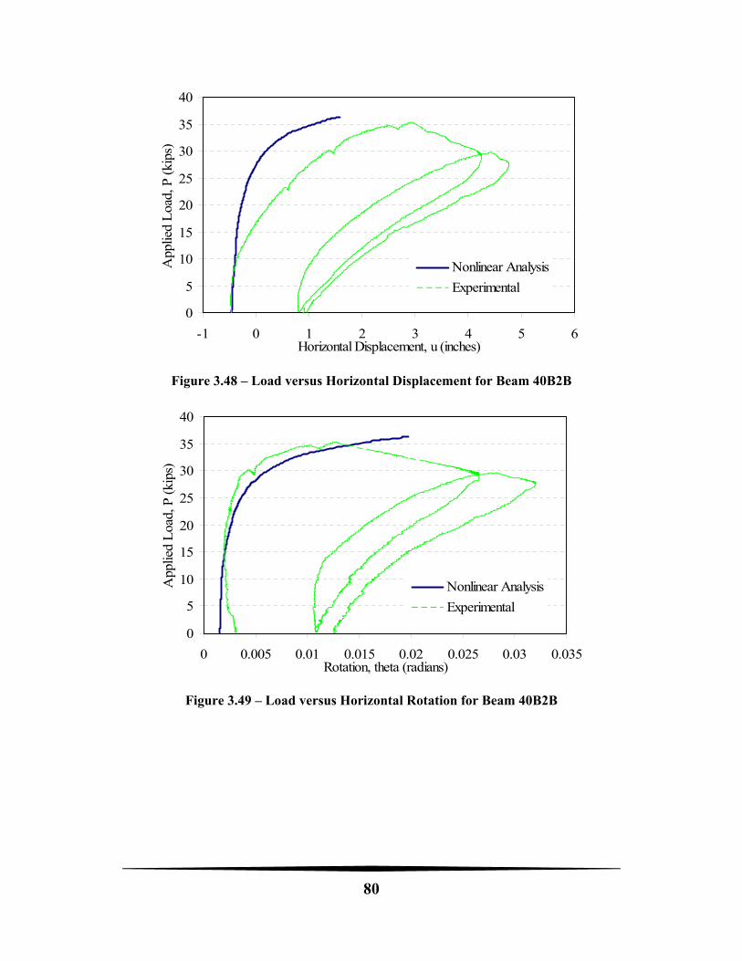
80

Figure 3.48 – Load versus Horizontal Displacement for Beam 40B2B

Figure 3.49 – Load versus Horizontal Rotation for Beam 40B2B

0

5

10

15

20

25

30

35

40

-1 0 1 2 3 4 5 6Horizontal Displacement, u (inches)

App

lied

Loa

d, P

(ki

ps)

Nonlinear Analysis

Experimental

0

5

10

15

20

25

30

35

40

0 0.005 0.01 0.015 0.02 0.025 0.03 0.035Rotation, theta (radians)

App

lied

Loa

d, P

(ki

ps)

Nonlinear Analysis

Experimental

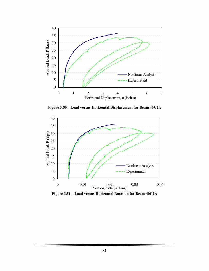
81

Figure 3.50 – Load versus Horizontal Displacement for Beam 40C2A

Figure 3.51 – Load versus Horizontal Rotation for Beam 40C2A

0

5

10

15

20

25

30

35

40

0 1 2 3 4 5 6 7Horizontal Displacement, u (inches)

App

lied

Loa

d, P

(ki

ps)

Nonlinear Analysis

Experimental

0

5

10

15

20

25

30

35

40

0 0.01 0.02 0.03 0.04Rotation, theta (radians)

App

lied

Loa

d, P

(ki

ps)

Nonlinear Analysis

Experimental

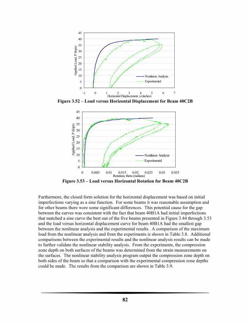
82

Figure 3.52 – Load versus Horizontal Displacement for Beam 40C2B

Figure 3.53 – Load versus Horizontal Rotation for Beam 40C2B

Furthermore, the closed form solution for the horizontal displacement was based on initial imperfections varying as a sine function. For some beams it was reasonable assumption and for other beams there were some significant differences. This potential cause for the gap between the curves was consistent with the fact that beam 40B1A had initial imperfections that matched a sine curve the best out of the five beams presented in Figure 3.44 through 3.53 and the load versus horizontal displacement curve for beam 40B1A had the smallest gap between the nonlinear analysis and the experimental results. A comparison of the maximum load from the nonlinear analysis and from the experiments is shown in Table 3.8. Additional comparisons between the experimental results and the nonlinear analysis results can be made to further validate the nonlinear stability analysis. From the experiments, the compression zone depth on both surfaces of the beams was determined from the strain measurements on the surfaces. The nonlinear stability analysis program output the compression zone depth on both sides of the beam so that a comparison with the experimental compression zone depths could be made. The results from the comparison are shown in Table 3.9.

0

5

10

15

20

25

30

35

40

45

-1 0 1 2 3 4 5 6 7Horizontal Displacement, u (inches)

App

lied

Loa

d, P

(ki

ps)

Nonlinear Analysis

Experimental

0

5

10

15

20

25

30

35

40

45

0 0.005 0.01 0.015 0.02 0.025 0.03 0.035Rotation, theta (radians)

App

lied

Loa

d, P

(ki

ps)

Nonlinear Analysis

Experimental

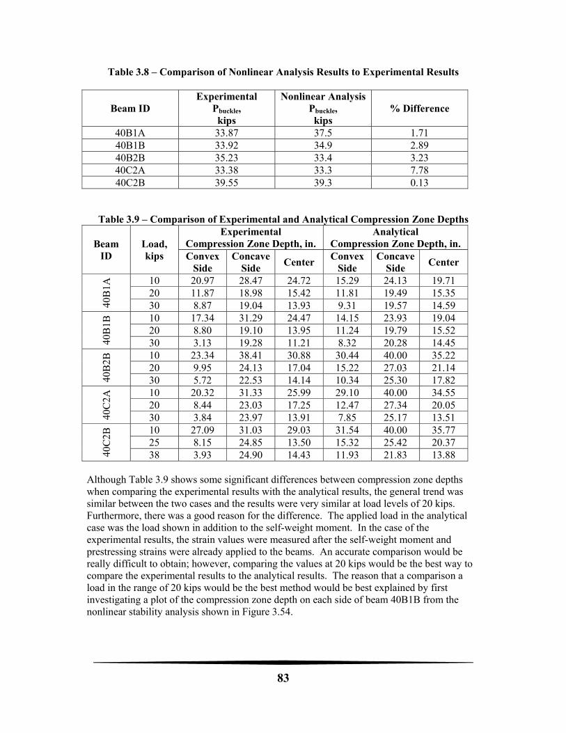
83

Table 3.8 – Comparison of Nonlinear Analysis Results to Experimental Results

Beam ID Experimental

Pbuckle, kips

Nonlinear AnalysisPbuckle, kips

% Difference

40B1A 33.87 37.5 1.71 40B1B 33.92 34.9 2.89 40B2B 35.23 33.4 3.23 40C2A 33.38 33.3 7.78 40C2B 39.55 39.3 0.13

Table 3.9 – Comparison of Experimental and Analytical Compression Zone Depths

Beam ID

Load, kips

Experimental Compression Zone Depth, in.

Analytical Compression Zone Depth, in.

Convex Side

Concave Side

Center Convex

Side Concave

Side Center

40B

1A

10 20.97 28.47 24.72 15.29 24.13 19.71 20 11.87 18.98 15.42 11.81 19.49 15.35 30 8.87 19.04 13.93 9.31 19.57 14.59

40B

1B

10 17.34 31.29 24.47 14.15 23.93 19.04 20 8.80 19.10 13.95 11.24 19.79 15.52 30 3.13 19.28 11.21 8.32 20.28 14.45

40B

2B

10 23.34 38.41 30.88 30.44 40.00 35.22 20 9.95 24.13 17.04 15.22 27.03 21.14 30 5.72 22.53 14.14 10.34 25.30 17.82

40C

2A

10 20.32 31.33 25.99 29.10 40.00 34.55 20 8.44 23.03 17.25 12.47 27.34 20.05 30 3.84 23.97 13.91 7.85 25.17 13.51

40C

2B

10 27.09 31.03 29.03 31.54 40.00 35.77 25 8.15 24.85 13.50 15.32 25.42 20.37 38 3.93 24.90 14.43 11.93 21.83 13.88

Although Table 3.9 shows some significant differences between compression zone depths when comparing the experimental results with the analytical results, the general trend was similar between the two cases and the results were very similar at load levels of 20 kips. Furthermore, there was a good reason for the difference. The applied load in the analytical case was the load shown in addition to the self-weight moment. In the case of the experimental results, the strain values were measured after the self-weight moment and prestressing strains were already applied to the beams. An accurate comparison would be really difficult to obtain; however, comparing the values at 20 kips would be the best way to compare the experimental results to the analytical results. The reason that a comparison a load in the range of 20 kips would be the best method would be best explained by first investigating a plot of the compression zone depth on each side of beam 40B1B from the nonlinear stability analysis shown in Figure 3.54.

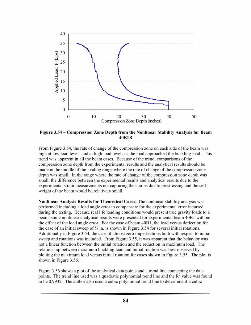
84

Figure 3.54 – Compression Zone Depth from the Nonlinear Stability Analysis for Beam 40B1B

From Figure 3.54, the rate of change of the compression zone on each side of the beam was high at low load levels and at high load levels as the load approached the buckling load. This trend was apparent in all the beam cases. Because of the trend, comparisons of the compression zone depth from the experimental results and the analytical results should be made in the middle of the loading range where the rate of change of the compression zone depth was small. In the range where the rate of change of the compression zone depth was small, the difference between the experimental results and analytical results due to the experimental strain measurements not capturing the strains due to prestressing and the self-weight of the beam would be relatively small.

Nonlinear Analysis Results for Theoretical Cases: The nonlinear stability analysis was performed including a load angle error to compensate for the experimental error incurred during the testing. Because real life loading conditions would present true gravity loads to a beam, some nonlinear analytical results were presented for experimental beam 40B1 without the effect of the load angle error. For the case of beam 40B1, the load versus deflection for the case of an initial sweep of ¼ in. is shown in Figure 3.54 for several initial rotations. Additionally in Figure 3.54, the case of almost zero imperfections both with respect to initial sweep and rotations was included. From Figure 3.55, it was apparent that the behavior was not a linear function between the initial rotation and the reduction in maximum load. The relationship between maximum buckling load and initial rotation was best observed by plotting the maximum load versus initial rotation for cases shown in Figure 3.55. The plot is shown in Figure 3.56. Figure 3.56 shows a plot of the analytical data points and a trend line connecting the data points. The trend line used was a quadratic polynomial trend line and the R2 value was found to be 0.9932. The author also used a cubic polynomial trend line to determine if a cubic

0

5

10

15

20

25

30

35

40

0 10 20 30 40 50Compression Zone Depth (inches)

App

lied

Loa

d, P

(ki

ps)

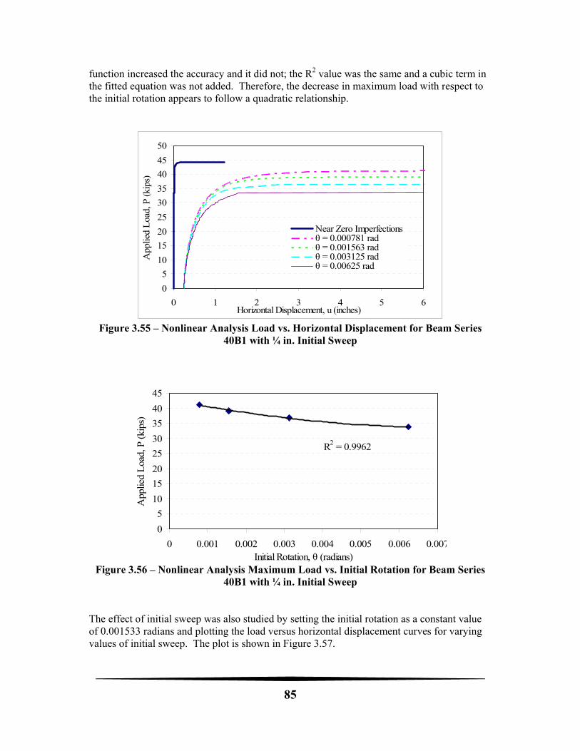
85

function increased the accuracy and it did not; the R2 value was the same and a cubic term in the fitted equation was not added. Therefore, the decrease in maximum load with respect to the initial rotation appears to follow a quadratic relationship.

Figure 3.55 – Nonlinear Analysis Load vs. Horizontal Displacement for Beam Series

40B1 with ¼ in. Initial Sweep

Figure 3.56 – Nonlinear Analysis Maximum Load vs. Initial Rotation for Beam Series

40B1 with ¼ in. Initial Sweep The effect of initial sweep was also studied by setting the initial rotation as a constant value of 0.001533 radians and plotting the load versus horizontal displacement curves for varying values of initial sweep. The plot is shown in Figure 3.57.

0

5

10

15

20

25

30

35

40

45

50

0 1 2 3 4 5 6Horizontal Displacement, u (inches)

App

lied

Loa

d, P

(ki

ps)

Near Zero Imperfectionsθ = 0.000781 radθ = 0.001563 radθ = 0.003125 radθ = 0.00625 rad

R2 = 0.9962

0

5

10

15

20

25

30

35

40

45

0 0.001 0.002 0.003 0.004 0.005 0.006 0.007Initial Rotation, θ (radians)

App

lied

Loa

d, P

(ki

ps)

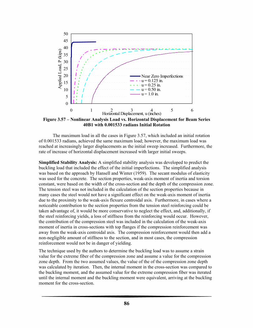
86

Figure 3.57 – Nonlinear Analysis Load vs. Horizontal Displacement for Beam Series

40B1 with 0.001533 radians Initial Rotation

The maximum load in all the cases in Figure 3.57, which included an initial rotation of 0.001533 radians, achieved the same maximum load; however, the maximum load was reached at increasingly larger displacements as the initial sweep increased. Furthermore, the rate of increase of horizontal displacement increased with larger initial sweeps.

Simplified Stability Analysis: A simplified stability analysis was developed to predict the buckling load that included the effect of the initial imperfections. The simplified analysis was based on the approach by Hansell and Winter (1959). The secant modulus of elasticity was used for the concrete. The section properties, weak-axis moment of inertia and torsion constant, were based on the width of the cross-section and the depth of the compression zone. The tension steel was not included in the calculation of the section properties because in many cases the steel would not have a significant effect on the weak-axis moment of inertia due to the proximity to the weak-axis flexure centroidal axis. Furthermore, in cases where a noticeable contribution to the section properties from the tension steel reinforcing could be taken advantage of, it would be more conservative to neglect the effect, and, additionally, if the steel reinforcing yields, a loss of stiffness from the reinforcing would occur. However, the contribution of the compression steel was included in the calculation of the weak-axis moment of inertia in cross-sections with top flanges if the compression reinforcement was away from the weak-axis centroidal axis. The compression reinforcement would then add a non-negligible amount of stiffness to the section, and in most cases, the compression reinforcement would not be in danger of yielding.

The technique used by the authors to determine the buckling load was to assume a strain value for the extreme fiber of the compression zone and assume a value for the compression zone depth. From the two assumed values, the value of the of the compression zone depth was calculated by iteration. Then, the internal moment in the cross-section was compared to the buckling moment, and the assumed value for the extreme compression fiber was iterated until the internal moment and the buckling moment were equivalent, arriving at the buckling moment for the cross-section.

0

5

10

15

20

25

30

35

40

45

50

0 1 2 3 4 5 6Horizontal Displacement, u (inches)

App

lied

Loa

d, P

(ki

ps)

Near Zero Imperfectionsu = 0.125 in.u = 0.25 in.u = 0.50 in.u = 1.0 in.

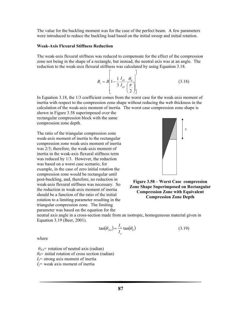
87

Figure 3.58 – Worst Case compression

Zone Shape Superimposed on Rectangular Compression Zone with Equivalent

Compression Zone Depth

The value for the buckling moment was for the case of the perfect beam. A few parameters were introduced to reduce the buckling load based on the initial sweep and initial rotation. Weak-Axis Flexural Stiffness Reduction The weak-axis flexural stiffness was reduced to compensate for the effect of the compression zone not being in the shape of a rectangle, but instead, the neutral axis was at an angle. The reduction to the weak-axis flexural stiffness was calculated by using Equation 3.18.

23

11 0

gy

gxr I

IBB (3.18)

In Equation 3.18, the 1/3 coefficient comes from the worst case for the weak-axis moment of inertia with respect to the compression zone shape without reducing the web thickness in the calculation of the weak-axis moment of inertia. The worst case compression zone shape is shown in Figure 3.58 superimposed over the rectangular compression block with the same compression zone depth.

The ratio of the triangular compression zone weak-axis moment of inertia to the rectangular compression zone weak-axis moment of inertia was 2/3; therefore, the weak-axis moment of inertia in the weak-axis flexural stiffness term was reduced by 1/3. However, the reduction was based on a worst case scenario, for example, in the case of zero initial rotation the compression zone would be rectangular until post-buckling, and, therefore, no reduction in weak-axis flexural stiffness was necessary. So the reduction in weak-axis moment of inertia should be a function of the ratio of the initial rotation to a limiting parameter resulting in the triangular compression zone. The limiting parameter was based on the equation for the neutral axis angle in a cross-section made from an isotropic, homogeneous material given in Equation 3.19 (Beer, 2001).

0tantan y

xNA I

I (3.19)

where θNA= rotation of neutral axis (radian) θ0= initial rotation of cross section (radian) Ix= strong axis moment of inertia Iy= weak axis moment of inertia

88

The worst case for the neutral axis for the triangular compression zone was a function of the geometry of the cross-section and the depth of the compression zone; therefore, to simplify, the worst case for the neutral axis angle was taken to be π/2. Rearranging Equation 3.19 arrived at the limiting initial rotation to be Equation 3.20.

x

y

I

I

2

0 (3.20)

Note that in the case of flanged cross-sections, more initial rotation would be necessary to affect the compression zone shape, and, therefore, reduce the weak-axis moment of inertia. However, the effect of flanges was inherent to Equation 3.15 because in a flanged cross-section, the gross weak-axis moment of inertia would increase dramatically, and, thus, decrease the reduction of the weak-axis stiffness in Equation 3.15. Buckling Load Reduction for Initial Imperfections: The buckling load was reduced due to initial imperfections besides the effect of the compression zone shape. The buckling load reduction for the effect of initial sweep was derived by considering the cubic relationship shown in Figure 3.58. Furthermore, the effect that an initial sweep would have on the torsion on the cross-section could be considered as a ratio of the sweep to the length. The reason for the conclusion was that the torque at midspan due to the initial sweep was the product of the applied load and the initial sweep. Furthermore, the torsional stress developed at the end of the beam was a linear function of the applied torque and the length of the beam. Because of the cubic relationship between the buckling load and the initial sweep, the reduction parameter (Δr) was derived as the cube root of the ratio of the initial sweep (δ0) to the length of the beam as shown in Equation 3.21.

3

1

01

Lr

(3.21)

Similarly to the derivation of the reduction of the buckling load due to an initial sweep a reduction due to the initial rotation (Θr), was derived based on the quadratic relationship between the buckling load and the initial rotation. Equation 3.22 is the resulting reduction parameter due to an initial rotation.

01 r (3.22)

Total Buckling Equation Including Initial Imperfection Effects: The total critical buckling moment equation for a simply-supported beam condition considering the parameters including the initial imperfections is as follows:

bimperfections r r rM B CL

(3.23)

In Eq. (3.23), the parameter “Α” was the parameter that takes into consideration the effect of load height on the buckling moment. Simplified Equation Results Compared to the Nonlinear Analysis: The simplified equation was used to predict the buckling load for beams with the geometry, mild reinforcing and prestressed reinforcing of the beam series’ 40C2 and 40B1 from this study with various

89

initial imperfections. The nonlinear analysis was also performed for all of the same cases so that a comparison was able to be made between the simplified analysis results and the nonlinear stability analysis results. The comparison is shown in Table 3.9. The simplified equation matched very well with the nonlinear stability analysis with a maximum percent difference for the cases presented of 4.5%. Furthermore, in every case the simplified equation over-predicted the analytical buckling load which was attributed to the fact that the simplified equation based the rigidity properties on the secant modulus of elasticity, while the nonlinear stability analysis used an average tangent modulus of the concrete elements in the compressed region. The average tangent modulus was always slightly lower than the secant modulus. Also, the buckling load from the nonlinear analysis was selected from the analytical data as the first load in which the horizontal displacements increased by more that ¼ in. in a 0.1 kip load increment. The selection was somewhat arbitrary; however, the author believed the maximum load from the nonlinear analysis, although in many cases was very close to the predicted buckling load using the simplified equation, was not a very good predictor of the buckling load because in many cases the maximum load was reached at horizontal displacement levels exceeding 5 in. Simplified Equation Results Compared to Experimental Results: Because the experimental results from this study include an effect of the error in the load application angle, the error in load application error was included as part of the initial rotation of the beam in the simplified equation. Furthermore, because the initial sweep of some of the beams was in the negative direction, which created a stabilizing effect, the initial sweeps that were negative were input into the simplified equation as zero value. The results of the comparison are shown in Table 3.10.

There was good correlation between the results from the experiments of this study and the predicted buckling loads using the simplified equation proposed in this study. However, the simplified equation was developed to determine buckling loads for beams with a perfect vertical load such as gravity load. To further validate the procedure, the simplified equation was also compared with the experimental results from König and Pauli (1990). The comparison is shown in Table 3.11.

In König and Pauli’s (1990) study, they varied the top flange width and the amount of compression reinforcement to parametrically study the effects using beams 1 through 4. Table 3.11 shows that the simplified equation arrived at predicted buckling loads very close to the experimental results. Beams 5 and 3 were both prestressed concrete beams. Beam 5 only had a top flange, while beam 3 included bottom flange. The simplified equation predicted the buckling loads well. The difference between the experimental results and predicted results for beams 5 and 3 were most likely due to the limited information published on the prestressing strands and prestressing force. Furthermore, the under-predicted buckling load from beam 3 probably stems from beam 3 having had a significantly greater amount of shear reinforcement in the cross-section than any of the other beams, and, furthermore, beam 3 included a significant amount of undesignated nominal longitudinal mild reinforcing steel throughout the cross-section that was not included in any of the other beams or in the analysis. Additionally, error in all beam cases could be attributed to the relative crudeness of the measured initial rotations.

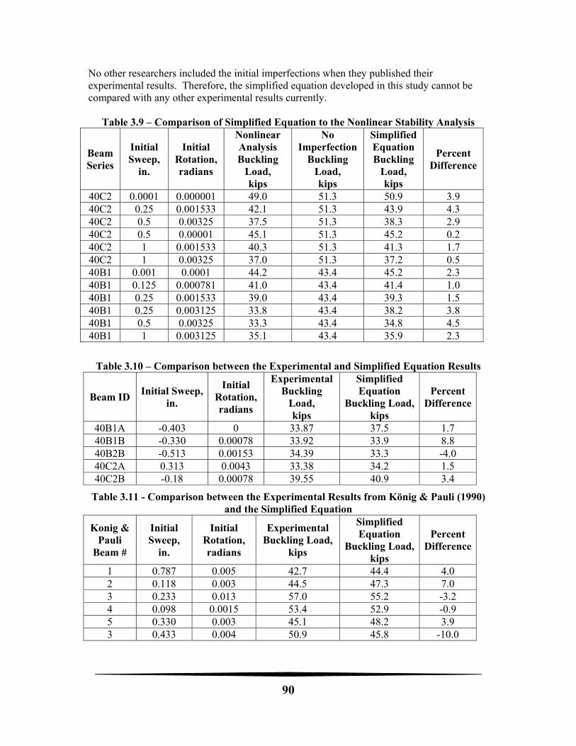
90

No other researchers included the initial imperfections when they published their experimental results. Therefore, the simplified equation developed in this study cannot be compared with any other experimental results currently.

Table 3.9 – Comparison of Simplified Equation to the Nonlinear Stability Analysis

Beam Series

Initial Sweep,

in.

Initial Rotation, radians

Nonlinear Analysis Buckling

Load, kips

No Imperfection

Buckling Load, kips

Simplified Equation Buckling

Load, kips

Percent Difference

40C2 0.0001 0.000001 49.0 51.3 50.9 3.9 40C2 0.25 0.001533 42.1 51.3 43.9 4.3 40C2 0.5 0.00325 37.5 51.3 38.3 2.9 40C2 0.5 0.00001 45.1 51.3 45.2 0.2 40C2 1 0.001533 40.3 51.3 41.3 1.7 40C2 1 0.00325 37.0 51.3 37.2 0.5 40B1 0.001 0.0001 44.2 43.4 45.2 2.3 40B1 0.125 0.000781 41.0 43.4 41.4 1.0 40B1 0.25 0.001533 39.0 43.4 39.3 1.5 40B1 0.25 0.003125 33.8 43.4 38.2 3.8 40B1 0.5 0.00325 33.3 43.4 34.8 4.5 40B1 1 0.003125 35.1 43.4 35.9 2.3

Table 3.10 – Comparison between the Experimental and Simplified Equation Results

Beam ID Initial Sweep,

in.

Initial Rotation,radians

ExperimentalBuckling

Load, kips

Simplified Equation

Buckling Load, kips

Percent Difference

40B1A -0.403 0 33.87 37.5 1.7 40B1B -0.330 0.00078 33.92 33.9 8.8 40B2B -0.513 0.00153 34.39 33.3 -4.0 40C2A 0.313 0.0043 33.38 34.2 1.5 40C2B -0.18 0.00078 39.55 40.9 3.4

Table 3.11 - Comparison between the Experimental Results from König & Pauli (1990) and the Simplified Equation

Konig & Pauli

Beam #

Initial Sweep,

in.

Initial Rotation, radians

Experimental Buckling Load,

kips

Simplified Equation

Buckling Load, kips

Percent Difference

1 0.787 0.005 42.7 44.4 4.0 2 0.118 0.003 44.5 47.3 7.0 3 0.233 0.013 57.0 55.2 -3.2 4 0.098 0.0015 53.4 52.9 -0.9 5 0.330 0.003 45.1 48.2 3.9 3 0.433 0.004 50.9 45.8 -10.0

91

Analytical Study of Prestressed Sections – Conclusions The developed nonlinear stability analysis proved to match the experimental load versus displacement and load versus rotation curves well. The nonlinear stability analysis was further expanded to beams of the same properties as the beam series 40B1, but with a series of different initial imperfections applied. The results from the nonlinear stability analysis were used to rationally determine the lateral-torsional buckling behavior of reinforced and prestressed concrete beams to develop an accurate simplified analysis to predict the lateral-torsional critical buckling moment of reinforced and prestressed concrete beams that included the effect of initial imperfections. The simplified equation to predict the buckling moment was verified by comparing the results from the simplified analysis with both the experimental results from this study as well as the experimental results from König and Pauli (1990), where actual gravity load was applied to the test specimens. In both cases, there was good correlation between the predicted buckling loads from the simplified equation and the experimentally determined buckling loads.

92

93

CHAPTER 4 ANALYTICAL INVESTIGATION OF THE THERMAL BEHAVIOR OF

A BT-54 PRESTRESSED CONCRETE GIRDER

Introduction

Concrete bridge structures are subjected to thermal loads due to their exposure to the environment. Solar radiation, the primary source of heat, causes the uneven heating of the concrete bridge. The nonlinear temperature distributions induced by the unbalanced heat flux generate an additional sweep that may lead to problems with torsional and lateral stability. However, the AASHTO Bridge Design Specifications (AASHTO, 1989; AASHTO, 2002; AASHTO, 2007) provide only vertical temperature distributions associated with environmental conditions, but rarely address temperature distributions related to the lateral thermal movement of the bridge.

This study is an analytical investigation of the temperature distributions and thermal

response of a precast, prestressed concrete BT-54 girder. The main objectives of this study are to determine hourly solar radiation incident on the surfaces of the concrete girder and to evaluate the thermal response considering the orientation of the bridge girder. The effects of seasonal variations and the orientation of the bridge axes on thermal behaviors are discussed with regard to four orientations of the bridge: a south-north, southeast-northwest, east-west, and northeast-southwest orientation.

Estimation of Seasonal Solar Radiation Daily Solar Radiation: Solar radiation is the main source of heat in concrete bridges under environmental conditions. Since the intensity of solar radiation changes over time, this research includes all four seasons of the year in its study of the variance in yearly solar radiation. The seasonal daily solar radiation, H , incident on a horizontal surface, was estimated by the average percent of possible sunshine hours (Jansen, 1985; Kreith, 1978; Threlkeld, 1970):

o

nH H a b

N

(4.1)

in which oH is extraterrestrial solar radiation, a and b location-dependent constants, 0.38 and 0.26 in Atlanta (Lof, 1966) and /n N the average percentage of possible sunshine hours (SRCC, 2009), 58%, 67%, 62%, and 50% for the spring, summer, fall, and winter in Atlanta, respectively. The daily extraterrestrial solar radiation, oH , was calculated by

86400 360

1 0.033cos cos cos sin sin sin365 180

sso sc ss

wnH G l d w l d

(4.2)

in which scG is a solar radiation constant equal to 1367 W/m2, n the day of the year, l the latitude of the site, d the declination of the sun, and ssw the hour angle of sunset (i.e., at 5

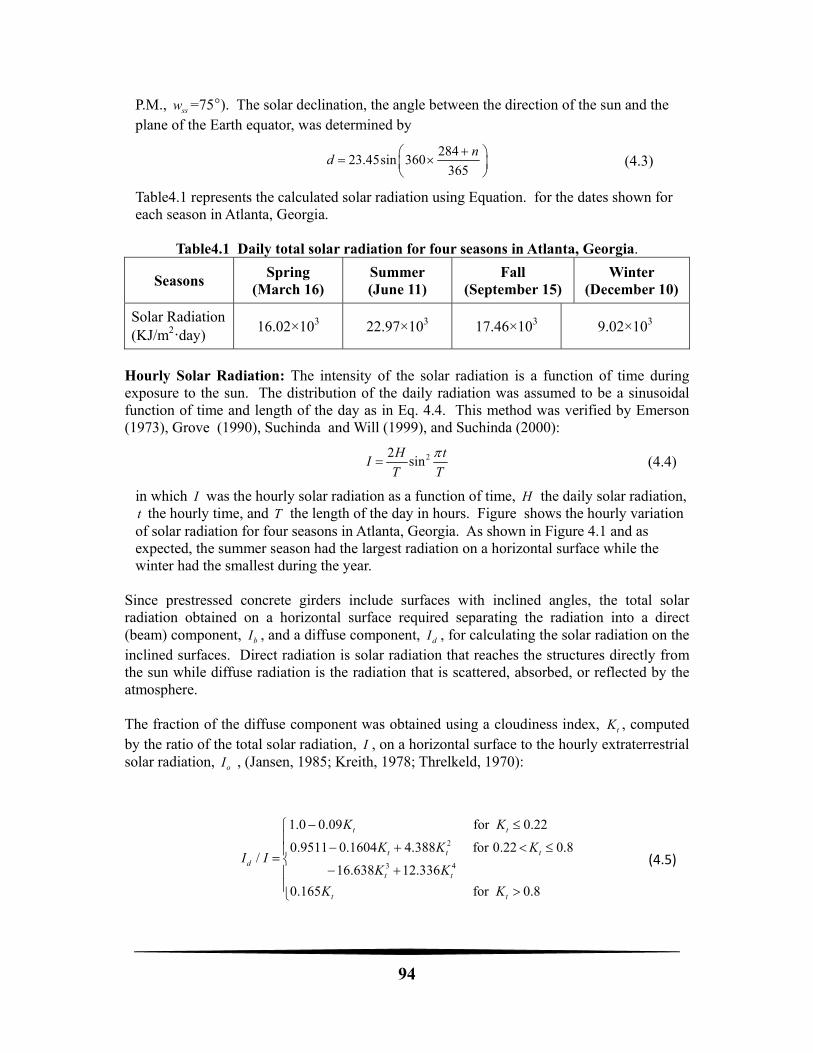
94

P.M., ssw =75°). The solar declination, the angle between the direction of the sun and the plane of the Earth equator, was determined by

284

23.45sin 360365

nd

(4.3)

Table4.1 represents the calculated solar radiation using Equation. for the dates shown for each season in Atlanta, Georgia.

Table4.1 Daily total solar radiation for four seasons in Atlanta, Georgia.

Seasons Spring

(March 16) Summer (June 11)

Fall (September 15)

Winter (December 10)

Solar Radiation (KJ/m2·day)

16.02×103 22.97×103 17.46×103 9.02×103

Hourly Solar Radiation: The intensity of the solar radiation is a function of time during exposure to the sun. The distribution of the daily radiation was assumed to be a sinusoidal function of time and length of the day as in Eq. 4.4. This method was verified by Emerson (1973), Grove (1990), Suchinda and Will (1999), and Suchinda (2000):

22

sinH t

IT T

(4.4)

in which I was the hourly solar radiation as a function of time, H the daily solar radiation, t the hourly time, and T the length of the day in hours. Figure shows the hourly variation of solar radiation for four seasons in Atlanta, Georgia. As shown in Figure 4.1 and as expected, the summer season had the largest radiation on a horizontal surface while the winter had the smallest during the year.

Since prestressed concrete girders include surfaces with inclined angles, the total solar radiation obtained on a horizontal surface required separating the radiation into a direct (beam) component, bI , and a diffuse component, dI , for calculating the solar radiation on the inclined surfaces. Direct radiation is solar radiation that reaches the structures directly from the sun while diffuse radiation is the radiation that is scattered, absorbed, or reflected by the atmosphere. The fraction of the diffuse component was obtained using a cloudiness index, tK , computed by the ratio of the total solar radiation, I , on a horizontal surface to the hourly extraterrestrial solar radiation, oI , (Jansen, 1985; Kreith, 1978; Threlkeld, 1970):

2

3 4

1.0 0.09 for 0.22

0.9511 0.1604 4.388 for 0.22 0.8/

16.638 12.336

0.165 for 0.8

t t

t t td

t t

t t

K K

K K KI I

K K

K K

  (4.5)

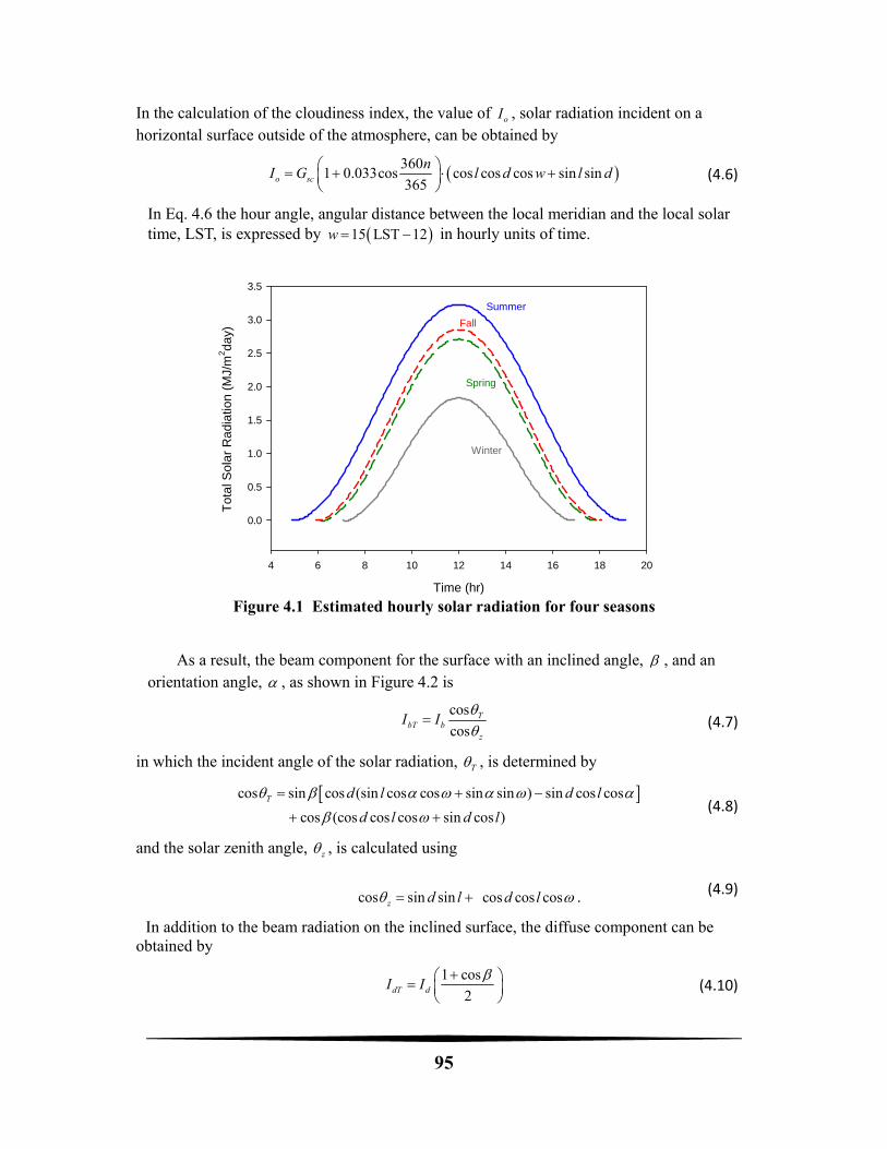
95

In the calculation of the cloudiness index, the value of oI , solar radiation incident on a horizontal surface outside of the atmosphere, can be obtained by

3601 0.033cos cos cos cos sin sin

365o sc

nI G l d w l d

(4.6)

In Eq. 4.6 the hour angle, angular distance between the local meridian and the local solar time, LST, is expressed by 15 LST 12w in hourly units of time.

Time (hr)

4 6 8 10 12 14 16 18 20

Tot

al S

ola

r R

adi

atio

n (

MJ/

m2 d

ay)

0.0

0.5

1.0

1.5

2.0

2.5

3.0

3.5

Summer

Winter

Fall

Spring

Figure 4.1 Estimated hourly solar radiation for four seasons

As a result, the beam component for the surface with an inclined angle, , and an orientation angle, , as shown in Figure 4.2 is

cos

cosT

bT bz

I I

  (4.7)

in which the incident angle of the solar radiation, T , is determined by

cos sin cos (sin cos cos sin sin ) sin cos cos

cos (cos cos cos sin cos )T d l d l

d l d l

  (4.8)

and the solar zenith angle, z , is calculated using

cos sin sinz d l cos cos cosd l .  (4.9)

In addition to the beam radiation on the inclined surface, the diffuse component can be obtained by

1 cos

2dT dI I

  (4.10)

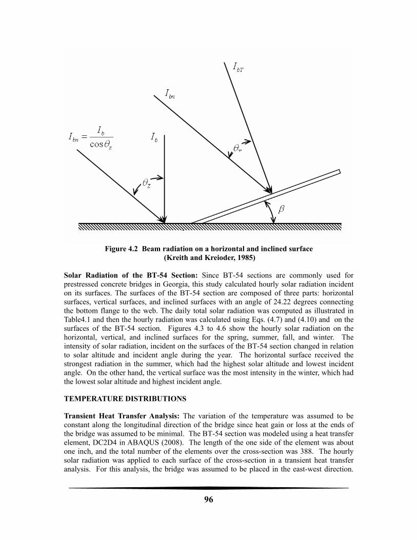
96

Figure 4.2 Beam radiation on a horizontal and inclined surface

(Kreith and Kreioder, 1985) Solar Radiation of the BT-54 Section: Since BT-54 sections are commonly used for prestressed concrete bridges in Georgia, this study calculated hourly solar radiation incident on its surfaces. The surfaces of the BT-54 section are composed of three parts: horizontal surfaces, vertical surfaces, and inclined surfaces with an angle of 24.22 degrees connecting the bottom flange to the web. The daily total solar radiation was computed as illustrated in Table4.1 and then the hourly radiation was calculated using Eqs. (4.7) and (4.10) and on the surfaces of the BT-54 section. Figures 4.3 to 4.6 show the hourly solar radiation on the horizontal, vertical, and inclined surfaces for the spring, summer, fall, and winter. The intensity of solar radiation, incident on the surfaces of the BT-54 section changed in relation to solar altitude and incident angle during the year. The horizontal surface received the strongest radiation in the summer, which had the highest solar altitude and lowest incident angle. On the other hand, the vertical surface was the most intensity in the winter, which had the lowest solar altitude and highest incident angle.

TEMPERATURE DISTRIBUTIONS

Transient Heat Transfer Analysis: The variation of the temperature was assumed to be constant along the longitudinal direction of the bridge since heat gain or loss at the ends of the bridge was assumed to be minimal. The BT-54 section was modeled using a heat transfer element, DC2D4 in ABAQUS (2008). The length of the one side of the element was about one inch, and the total number of the elements over the cross-section was 388. The hourly solar radiation was applied to each surface of the cross-section in a transient heat transfer analysis. For this analysis, the bridge was assumed to be placed in the east-west direction.

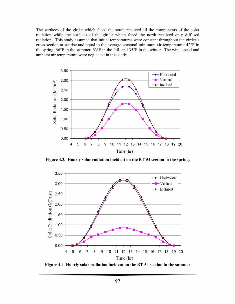
97

The surfaces of the girder which faced the south received all the components of the solar radiation while the surfaces of the girder which faced the north received only diffused radiation. This study assumed that initial temperatures were constant throughout the girder’s cross-section at sunrise and equal to the average seasonal minimum air temperature: 42°F in the spring, 66°F in the summer, 63°F in the fall, and 35°F in the winter. The wind speed and ambient air temperature were neglected in this study.

Figure 4.3. Hourly solar radiation incident on the BT-54 section in the spring.

Figure 4.4 Hourly solar radiation incident on the BT-54 section in the summer

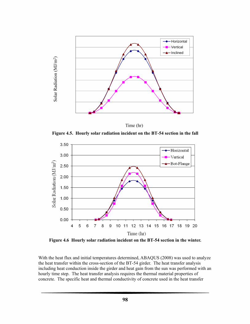
98

Figure 4.5. Hourly solar radiation incident on the BT-54 section in the fall

Figure 4.6 Hourly solar radiation incident on the BT-54 section in the winter.

With the heat flux and initial temperatures determined, ABAQUS (2008) was used to analyze the heat transfer within the cross-section of the BT-54 girder. The heat transfer analysis including heat conduction inside the girder and heat gain from the sun was performed with an hourly time step. The heat transfer analysis requires the thermal material properties of concrete. The specific heat and thermal conductivity of concrete used in the heat transfer

Sol

ar R

adia

tion

(M

J/m

2 )

Time (hr)

Horizontal

Vertical

Inclined

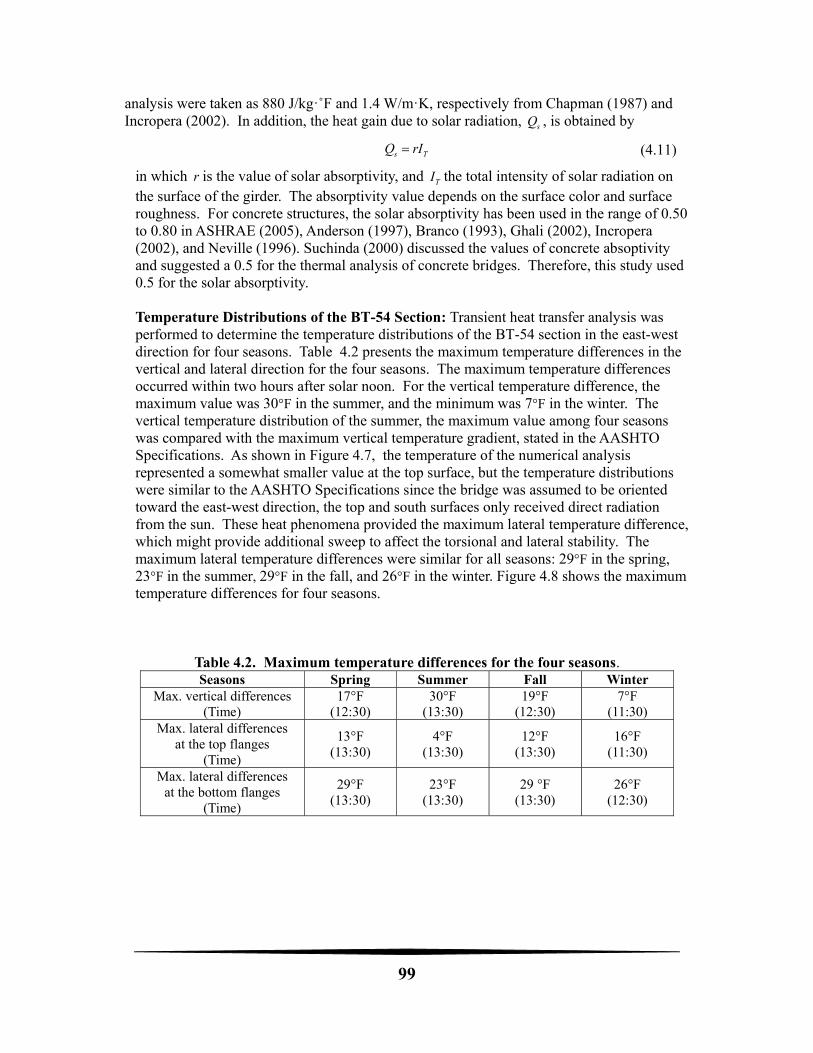
99

analysis were taken as 880 J/kg·˚F and 1.4 W/m·K, respectively from Chapman (1987) and Incropera (2002). In addition, the heat gain due to solar radiation, sQ , is obtained by

s TQ rI   (4.11)

in which r is the value of solar absorptivity, and TI the total intensity of solar radiation on the surface of the girder. The absorptivity value depends on the surface color and surface roughness. For concrete structures, the solar absorptivity has been used in the range of 0.50 to 0.80 in ASHRAE (2005), Anderson (1997), Branco (1993), Ghali (2002), Incropera (2002), and Neville (1996). Suchinda (2000) discussed the values of concrete absoptivity and suggested a 0.5 for the thermal analysis of concrete bridges. Therefore, this study used 0.5 for the solar absorptivity.

Temperature Distributions of the BT-54 Section: Transient heat transfer analysis was performed to determine the temperature distributions of the BT-54 section in the east-west direction for four seasons. Table 4.2 presents the maximum temperature differences in the vertical and lateral direction for the four seasons. The maximum temperature differences occurred within two hours after solar noon. For the vertical temperature difference, the maximum value was 30°F in the summer, and the minimum was 7°F in the winter. The vertical temperature distribution of the summer, the maximum value among four seasons was compared with the maximum vertical temperature gradient, stated in the AASHTO Specifications. As shown in Figure 4.7, the temperature of the numerical analysis represented a somewhat smaller value at the top surface, but the temperature distributions were similar to the AASHTO Specifications since the bridge was assumed to be oriented toward the east-west direction, the top and south surfaces only received direct radiation from the sun. These heat phenomena provided the maximum lateral temperature difference, which might provide additional sweep to affect the torsional and lateral stability. The maximum lateral temperature differences were similar for all seasons: 29°F in the spring, 23°F in the summer, 29°F in the fall, and 26°F in the winter. Figure 4.8 shows the maximum temperature differences for four seasons.

Table 4.2. Maximum temperature differences for the four seasons. Seasons Spring Summer Fall Winter

Max. vertical differences (Time)

17°F (12:30)

30°F (13:30)

19°F (12:30)

7°F (11:30)

Max. lateral differences at the top flanges

(Time)

13°F (13:30)

4°F (13:30)

12°F (13:30)

16°F (11:30)

Max. lateral differences at the bottom flanges

(Time)

29°F (13:30)

23°F (13:30)

29 °F (13:30)

26°F (12:30)

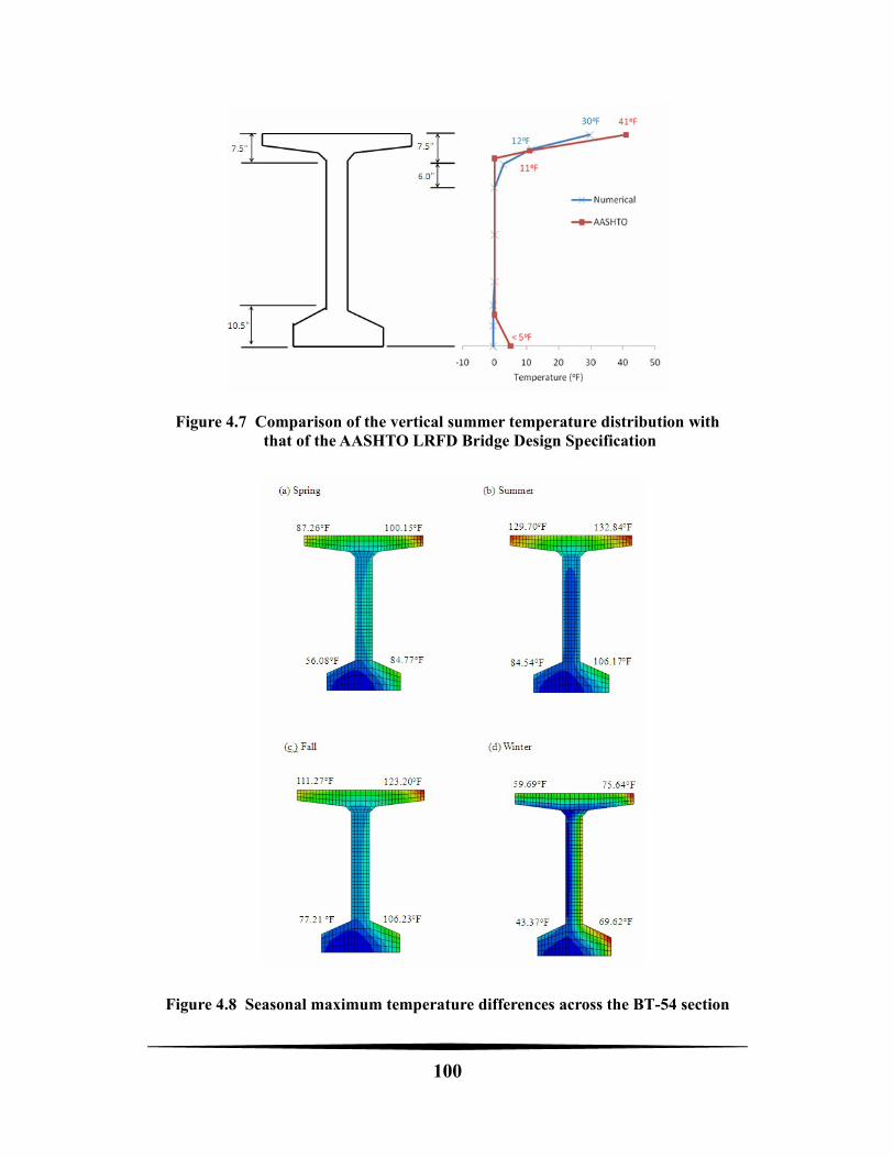
100

Figure 4.7 Comparison of the vertical summer temperature distribution with that of the AASHTO LRFD Bridge Design Specification

Figure 4.8 Seasonal maximum temperature differences across the BT-54 section

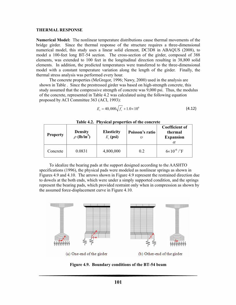
101

THERMAL RESPONSE Numerical Model: The nonlinear temperature distributions cause thermal movements of the bridge girder. Since the thermal response of the structure requires a three-dimensional numerical model, this study uses a linear solid element, DC3D8 in ABAQUS (2008), to model a 100-feet long BT-54 section. The cross-section of the girder, composed of 388 elements, was extended to 100 feet in the longitudinal direction resulting in 38,800 solid elements. In addition, the predicted temperatures were transferred to the three-dimensional model with a constant temperature variation along the length of the girder. Finally, the thermal stress analysis was performed every hour.

The concrete properties (McGregor, 1996; Nawy, 2000) used in the analysis are shown in Table . Since the prestressed girder was based on high-strength concrete, this study assumed that the compressive strength of concrete was 9,000 psi. Thus, the modulus of the concrete, represented in Table 4.2 was calculated using the following equation proposed by ACI Committee 363 (ACI, 1993):

' 640,000 1.0 10c cE f   (4.12)

Table 4.2. Physical properties of the concrete

Property Density (lb/in3)

Elasticity

cE (psi) Poisson’s ratio

Coefficient of thermal

Expansion

Concrete 0.0831 4,800,000 0.2 610-6 /˚F

To idealize the bearing pads at the support designed according to the AASHTO specifications (1996), the physical pads were modeled as nonlinear springs as shown in Figures 4.9 and 4.10. The arrows shown in Figure 4.9 represent the restrained direction due to dowels at the both ends, which were under a simply supported condition, and the springs represent the bearing pads, which provided restraint only when in compression as shown by the assumed force-displacement curve in Figure 4.10.

Figure 4.9. Boundary conditions of the BT-54 beam

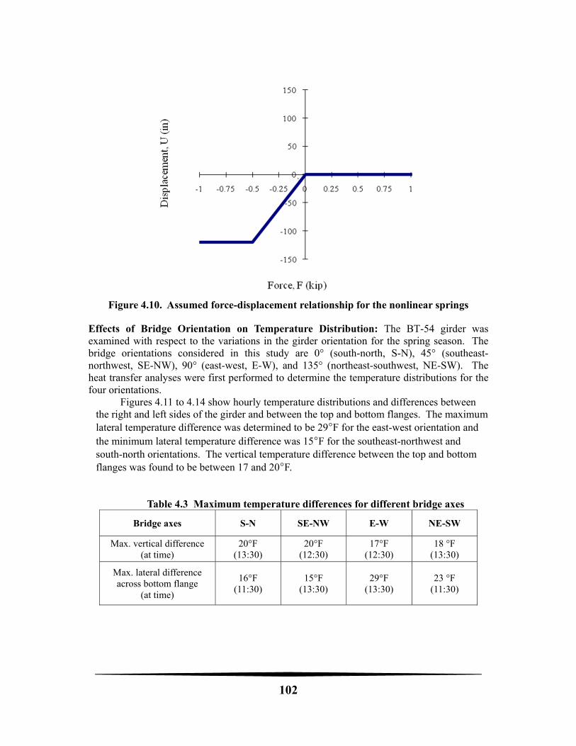
102

Figure 4.10. Assumed force-displacement relationship for the nonlinear springs

Effects of Bridge Orientation on Temperature Distribution: The BT-54 girder was examined with respect to the variations in the girder orientation for the spring season. The bridge orientations considered in this study are 0° (south-north, S-N), 45° (southeast-northwest, SE-NW), 90° (east-west, E-W), and 135° (northeast-southwest, NE-SW). The heat transfer analyses were first performed to determine the temperature distributions for the four orientations.

Figures 4.11 to 4.14 show hourly temperature distributions and differences between the right and left sides of the girder and between the top and bottom flanges. The maximum lateral temperature difference was determined to be 29°F for the east-west orientation and the minimum lateral temperature difference was 15°F for the southeast-northwest and south-north orientations. The vertical temperature difference between the top and bottom flanges was found to be between 17 and 20°F.

Table 4.3 Maximum temperature differences for different bridge axes

Bridge axes S-N SE-NW E-W NE-SW

Max. vertical difference (at time)

20°F (13:30)

20°F (12:30)

17°F (12:30)

18 °F (13:30)

Max. lateral difference across bottom flange

(at time)

16°F (11:30)

15°F (13:30)

29°F (13:30)

23 °F (11:30)

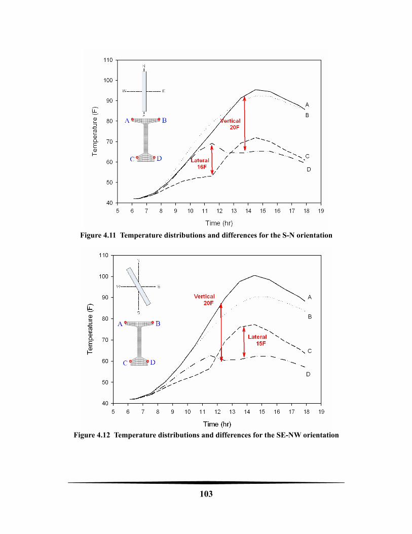
103

Figure 4.11 Temperature distributions and differences for the S-N orientation

Figure 4.12 Temperature distributions and differences for the SE-NW orientation

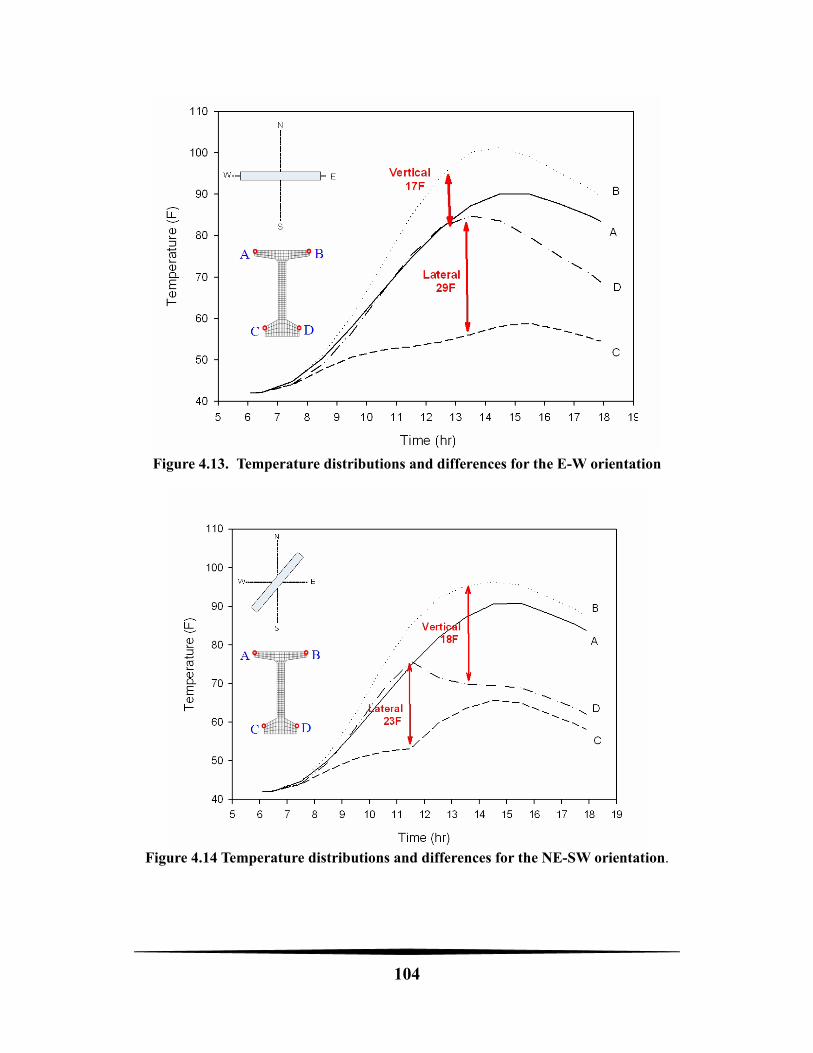
104

Figure 4.13. Temperature distributions and differences for the E-W orientation

Figure 4.14 Temperature distributions and differences for the NE-SW orientation.

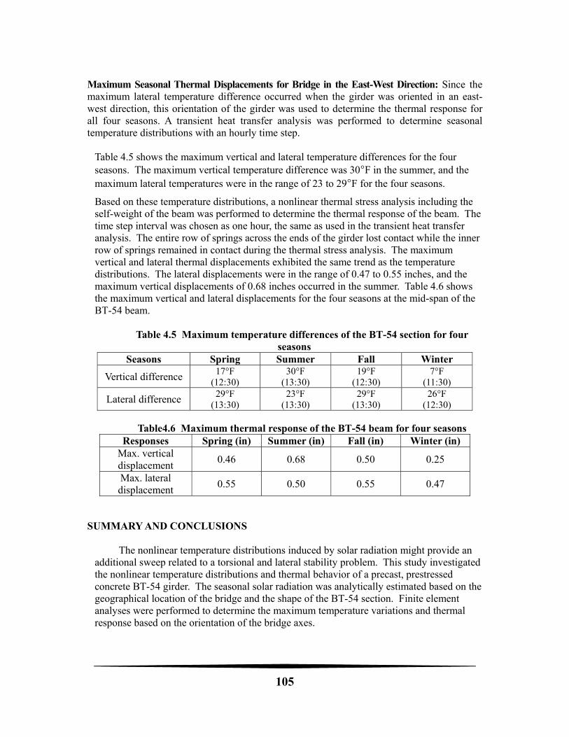
105

Maximum Seasonal Thermal Displacements for Bridge in the East-West Direction: Since the maximum lateral temperature difference occurred when the girder was oriented in an east-west direction, this orientation of the girder was used to determine the thermal response for all four seasons. A transient heat transfer analysis was performed to determine seasonal temperature distributions with an hourly time step.

Table 4.5 shows the maximum vertical and lateral temperature differences for the four seasons. The maximum vertical temperature difference was 30°F in the summer, and the maximum lateral temperatures were in the range of 23 to 29°F for the four seasons.

Based on these temperature distributions, a nonlinear thermal stress analysis including the self-weight of the beam was performed to determine the thermal response of the beam. The time step interval was chosen as one hour, the same as used in the transient heat transfer analysis. The entire row of springs across the ends of the girder lost contact while the inner row of springs remained in contact during the thermal stress analysis. The maximum vertical and lateral thermal displacements exhibited the same trend as the temperature distributions. The lateral displacements were in the range of 0.47 to 0.55 inches, and the maximum vertical displacements of 0.68 inches occurred in the summer. Table 4.6 shows the maximum vertical and lateral displacements for the four seasons at the mid-span of the BT-54 beam.

Table 4.5 Maximum temperature differences of the BT-54 section for four

seasons Seasons Spring Summer Fall Winter

Vertical difference 17°F (12:30)

30°F (13:30)

19°F (12:30)

7°F (11:30)

Lateral difference 29°F (13:30)

23°F (13:30)

29°F (13:30)

26°F (12:30)

Table4.6 Maximum thermal response of the BT-54 beam for four seasons Responses Spring (in) Summer (in) Fall (in) Winter (in)

Max. vertical displacement

0.46 0.68 0.50 0.25

Max. lateral displacement

0.55 0.50 0.55 0.47

SUMMARY AND CONCLUSIONS

The nonlinear temperature distributions induced by solar radiation might provide an additional sweep related to a torsional and lateral stability problem. This study investigated the nonlinear temperature distributions and thermal behavior of a precast, prestressed concrete BT-54 girder. The seasonal solar radiation was analytically estimated based on the geographical location of the bridge and the shape of the BT-54 section. Finite element analyses were performed to determine the maximum temperature variations and thermal response based on the orientation of the bridge axes.

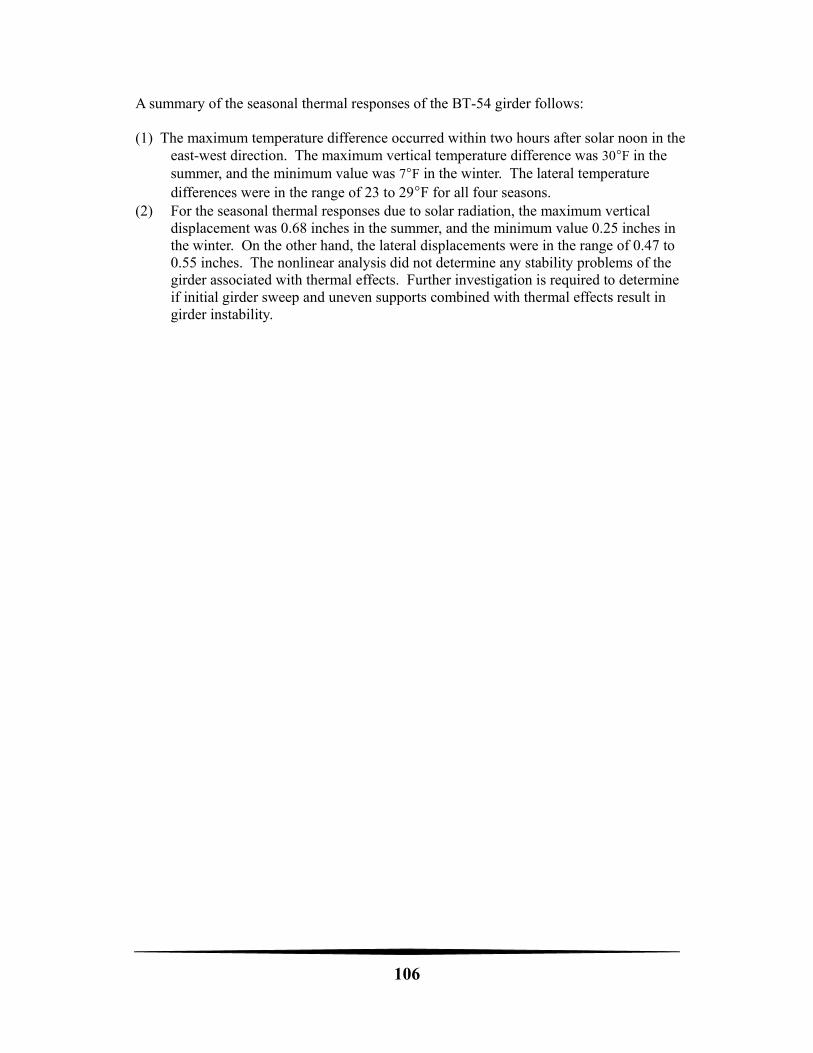
106

A summary of the seasonal thermal responses of the BT-54 girder follows: (1) The maximum temperature difference occurred within two hours after solar noon in the

east-west direction. The maximum vertical temperature difference was 30°F in the summer, and the minimum value was 7°F in the winter. The lateral temperature differences were in the range of 23 to 29°F for all four seasons.

(2) For the seasonal thermal responses due to solar radiation, the maximum vertical displacement was 0.68 inches in the summer, and the minimum value 0.25 inches in the winter. On the other hand, the lateral displacements were in the range of 0.47 to 0.55 inches. The nonlinear analysis did not determine any stability problems of the girder associated with thermal effects. Further investigation is required to determine if initial girder sweep and uneven supports combined with thermal effects result in girder instability.

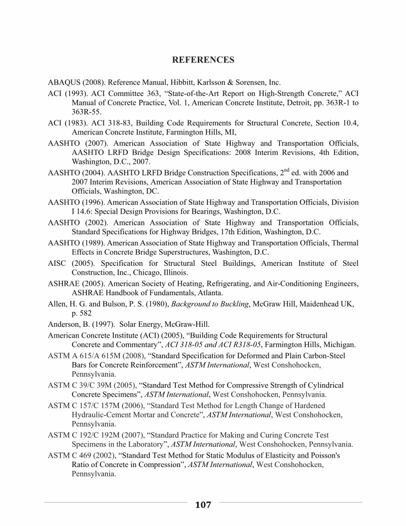
107

REFERENCES

ABAQUS (2008). Reference Manual, Hibbitt, Karlsson & Sorensen, Inc.

ACI (1993). ACI Committee 363, “State-of-the-Art Report on High-Strength Concrete,” ACI Manual of Concrete Practice, Vol. 1, American Concrete Institute, Detroit, pp. 363R-1 to 363R-55.

ACI (1983). ACI 318-83, Building Code Requirements for Structural Concrete, Section 10.4, American Concrete Institute, Farmington Hills, MI,

AASHTO (2007). American Association of State Highway and Transportation Officials, AASHTO LRFD Bridge Design Specifications: 2008 Interim Revisions, 4th Edition, Washington, D.C., 2007.

AASHTO (2004). AASHTO LRFD Bridge Construction Specifications, 2nd ed. with 2006 and 2007 Interim Revisions, American Association of State Highway and Transportation Officials, Washington, DC.

AASHTO (1996). American Association of State Highway and Transportation Officials, Division I 14.6: Special Design Provisions for Bearings, Washington, D.C.

AASHTO (2002). American Association of State Highway and Transportation Officials, Standard Specifications for Highway Bridges, 17th Edition, Washington, D.C.

AASHTO (1989). American Association of State Highway and Transportation Officials, Thermal Effects in Concrete Bridge Superstructures, Washington, D.C.

AISC (2005). Specification for Structural Steel Buildings, American Institute of Steel Construction, Inc., Chicago, Illinois.

ASHRAE (2005). American Society of Heating, Refrigerating, and Air-Conditioning Engineers, ASHRAE Handbook of Fundamentals, Atlanta.

Allen, H. G. and Bulson, P. S. (1980), Background to Buckling, McGraw Hill, Maidenhead UK, p. 582

Anderson, B. (1997). Solar Energy, McGraw-Hill.

American Concrete Institute (ACI) (2005), “Building Code Requirements for Structural Concrete and Commentary”, ACI 318-05 and ACI R318-05, Farmington Hills, Michigan.

ASTM A 615/A 615M (2008), “Standard Specification for Deformed and Plain Carbon-Steel Bars for Concrete Reinforcement”, ASTM International, West Conshohocken, Pennsylvania.

ASTM C 39/C 39M (2005), “Standard Test Method for Compressive Strength of Cylindrical Concrete Specimens”, ASTM International, West Conshohocken, Pennsylvania.

ASTM C 157/C 157M (2006), “Standard Test Method for Length Change of Hardened Hydraulic-Cement Mortar and Concrete”, ASTM International, West Conshohocken, Pennsylvania.

ASTM C 192/C 192M (2007), “Standard Practice for Making and Curing Concrete Test Specimens in the Laboratory”, ASTM International, West Conshohocken, Pennsylvania.

ASTM C 469 (2002), “Standard Test Method for Static Modulus of Elasticity and Poisson's Ratio of Concrete in Compression”, ASTM International, West Conshohocken, Pennsylvania.

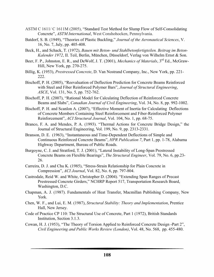
108

ASTM C 1611/ C 1611M (2005), “Standard Test Method for Slump Flow of Self-Consolidating Concrete”, ASTM International, West Conshohocken, Pennsylvania.

Batdorf, S. B. (1949), “Theories of Plastic Buckling,” Journal of the Aeronautical Sciences, V. 16, No. 7, July, pp. 405-408.

Beck, H., and Schack, T. (1972), Bauen mit Beton- und Stahlbetonfertigteilen. Beitrag im Beton-Kalender 1972, II. Teil, Berlin, München, Düsseldorf, Verlag von Wilhelm Ernst & Son.

Beer, F. P., Johnston, E. R., and DeWolf, J. T. (2001), Mechanics of Materials, 3rd Ed., McGraw-Hill, New York, pp. 270-275.

Billig, K. (1953), Prestressed Concrete, D. Van Nostrand Company, Inc., New York, pp. 221-222.

Bischoff, P. H. (2005), “Reevaluation of Deflection Prediction for Concrete Beams Reinforced with Steel and Fiber Reinforced Polymer Bars”, Journal of Structural Engineering, ASCE, Vol. 131, No. 5, pp. 752-762.

Bischoff, P. H. (2007), “Rational Model for Calculating Deflection of Reinforced Concrete Beams and Slabs”, Canadian Journal of Civil Engineering, Vol. 34, No. 8, pp. 992-1002.

Bischoff, P. H. and Scanlon A. (2007), “Effective Moment of Inertia for Calculating Deflections of Concrete Members Containing Steel Reinforcement and Fiber-Reinforced Polymer Reinforcement”, ACI Structural Journal, Vol. 104, No. 1, pp. 68-75.

Branco, F. A. and Mendes, P. A. (1993). “Thermal Actions for Concrete Bridge Design,” the Journal of Structural Engineering, Vol. 199, No. 9, pp. 2313-2331.

Branson, D. E. (1963), “Instantaneous and Time-Dependent Deflections of Simple and Continuous Reinforced Concrete Beams”, HPR Publication 7, Part 1, pp. 1-78, Alabama Highway Department, Bureau of Public Roads.

Burgoyne, C. J. and Stratford, T. J. (2001), “Lateral Instability of Long-Span Prestressed Concrete Beams on Flexible Bearings”, The Structural Engineer, Vol. 79, No. 6, pp.23-26.

Carreira, D. J. and Chu K. (1985), “Stress-Strain Relationship for Plain Concrete in Compression”, ACI Journal, Vol. 82, No. 6, pp. 797-804.

Castrodale, Reid W. and White, Christopher D. (2004). “Extending Span Ranges of Precast Prestressed Concrete Girders,” NCHRP Report 517, Transportation Research Board, Washington, D.C.

Chapman, A. J. (1987). Fundamentals of Heat Transfer, Macmillan Publishing Company, New York.

Chen, W. F., and Lui, E. M. (1987), Structural Stability: Theory and Implementation, Prentice Hall, New Jersey.

Code of Practice CP 110: The Structural Use of Concrete, Part 1 (1972), British Standards Institution, Section 3.1.3.

Cowan, H. J. (1953), “The Theory of Torsion Applied to Reinforced Concrete Design -Part 2”, Civil Engineering and Public Works Review (London), Vol. 48, No. 568, pp. 455-480.

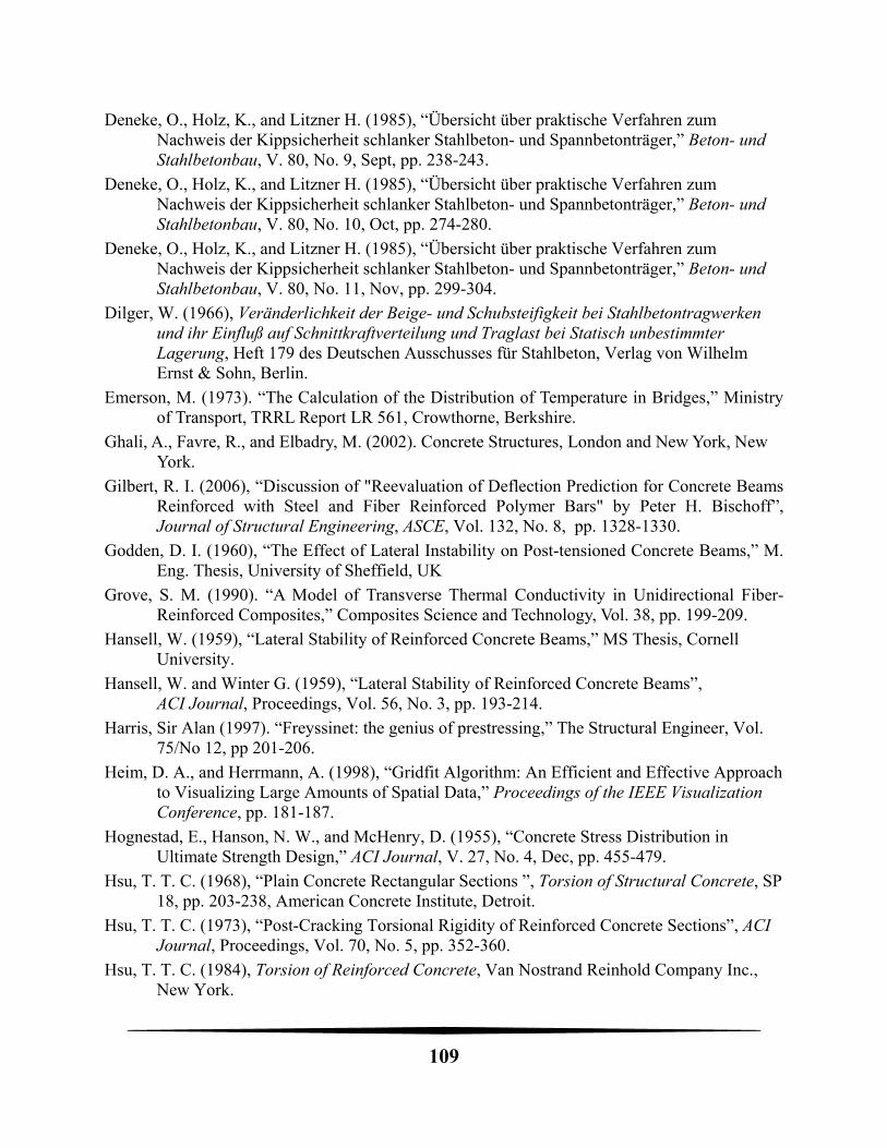
109

Deneke, O., Holz, K., and Litzner H. (1985), “Übersicht über praktische Verfahren zum Nachweis der Kippsicherheit schlanker Stahlbeton- und Spannbetonträger,” Beton- und Stahlbetonbau, V. 80, No. 9, Sept, pp. 238-243.

Deneke, O., Holz, K., and Litzner H. (1985), “Übersicht über praktische Verfahren zum Nachweis der Kippsicherheit schlanker Stahlbeton- und Spannbetonträger,” Beton- und Stahlbetonbau, V. 80, No. 10, Oct, pp. 274-280.

Deneke, O., Holz, K., and Litzner H. (1985), “Übersicht über praktische Verfahren zum Nachweis der Kippsicherheit schlanker Stahlbeton- und Spannbetonträger,” Beton- und Stahlbetonbau, V. 80, No. 11, Nov, pp. 299-304.

Dilger, W. (1966), Veränderlichkeit der Beige- und Schubsteifigkeit bei Stahlbetontragwerken und ihr Einfluß auf Schnittkraftverteilung und Traglast bei Statisch unbestimmter Lagerung, Heft 179 des Deutschen Ausschusses für Stahlbeton, Verlag von Wilhelm Ernst & Sohn, Berlin.

Emerson, M. (1973). “The Calculation of the Distribution of Temperature in Bridges,” Ministry of Transport, TRRL Report LR 561, Crowthorne, Berkshire.

Ghali, A., Favre, R., and Elbadry, M. (2002). Concrete Structures, London and New York, New York.

Gilbert, R. I. (2006), “Discussion of "Reevaluation of Deflection Prediction for Concrete Beams Reinforced with Steel and Fiber Reinforced Polymer Bars" by Peter H. Bischoff”, Journal of Structural Engineering, ASCE, Vol. 132, No. 8, pp. 1328-1330.

Godden, D. I. (1960), “The Effect of Lateral Instability on Post-tensioned Concrete Beams,” M. Eng. Thesis, University of Sheffield, UK

Grove, S. M. (1990). “A Model of Transverse Thermal Conductivity in Unidirectional Fiber-Reinforced Composites,” Composites Science and Technology, Vol. 38, pp. 199-209.

Hansell, W. (1959), “Lateral Stability of Reinforced Concrete Beams,” MS Thesis, Cornell University.

Hansell, W. and Winter G. (1959), “Lateral Stability of Reinforced Concrete Beams”, ACI Journal, Proceedings, Vol. 56, No. 3, pp. 193-214.

Harris, Sir Alan (1997). “Freyssinet: the genius of prestressing,” The Structural Engineer, Vol. 75/No 12, pp 201-206.

Heim, D. A., and Herrmann, A. (1998), “Gridfit Algorithm: An Efficient and Effective Approach to Visualizing Large Amounts of Spatial Data,” Proceedings of the IEEE Visualization Conference, pp. 181-187.

Hognestad, E., Hanson, N. W., and McHenry, D. (1955), “Concrete Stress Distribution in Ultimate Strength Design,” ACI Journal, V. 27, No. 4, Dec, pp. 455-479.

Hsu, T. T. C. (1968), “Plain Concrete Rectangular Sections ”, Torsion of Structural Concrete, SP 18, pp. 203-238, American Concrete Institute, Detroit.

Hsu, T. T. C. (1973), “Post-Cracking Torsional Rigidity of Reinforced Concrete Sections”, ACI Journal, Proceedings, Vol. 70, No. 5, pp. 352-360.

Hsu, T. T. C. (1984), Torsion of Reinforced Concrete, Van Nostrand Reinhold Company Inc., New York.

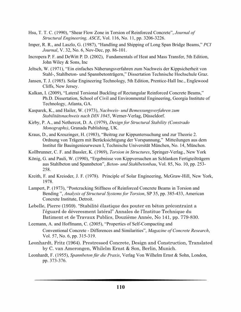
110

Hsu, T. T. C. (1990), “Shear Flow Zone in Torsion of Reinforced Concrete”, Journal of Structural Engineering, ASCE, Vol. 116, No. 11, pp. 3206-3226.

Imper, R. R., and Laszlo, G. (1987), “Handling and Shipping of Long Span Bridge Beams,” PCI Journal, V. 32, No. 6, Nov-Dec, pp. 86-101.

Incropera P. F. and DeWitt P. D. (2002), Fundamentals of Heat and Mass Transfer, 5th Edition, John Wiley & Sons, Inc

Jeltsch, W. (1971), “Ein einfaches Näherungsverfahren zum Nachweis der Kippsicherheit von Stahl-, Stahlbeton- und Spannbetonträgern,” Dissertation Technische Hochschule Graz.

Jansen, T. J. (1985). Solar Engineering Technology, 5th Edition, Prentice-Hall Inc., Englewood Cliffs, New Jersey.

Kalkan, I. (2009), “Lateral Torsional Buckling of Rectangular Reinforced Concrete Beams,” Ph.D. Dissertation, School of Civil and Environmental Engineering, Georgia Institute of Technology, Atlanta, GA.

Kasparek, K., and Hailer, W. (1973), Nachweis- und Bemessungsverfahren zum Stabilitätsnachweis nach DIN 1045, Werner-Verlag, Düsseldorf.

Kirby, P. A., and Nethercot, D. A. (1979), Design for Structural Stability (Constrado Monographs), Granada Publishing, UK.

Kraus, D., and Kreuzinger, H. (1983), “Beitrag zur Kippuntersuchung und zur Theorie 2. Ordnung von Trägern mit Berücksichtigung der Vorspannung,” Mitteilungen aus dem Institut für Bauingenieurwesen I, Technische Universität München, No. 14, München.

Kollbrunner, C. F. and Bassler, K. (1969), Torsion in Structures, Springer-Verlag., New York

König, G. and Pauli, W. (1990), “Ergebnisse von Kippversuchen an Schlanken Fertigteilträgern aus Stahlbeton und Spannbeton”, Beton- und Stahlbetonbau, Vol. 85, No. 10, pp. 253-258.

Kreith, F. and Kreioder, J. F. (1978). Principle of Solar Engineering, McGraw-Hill, New York, 1978.

Lampert, P. (1973), “Postcracking Stiffness of Reinforced Concrete Beams in Torsion and Bending ”, Analysis of Structural Systems for Torsion, SP 35, pp. 385-433, American Concrete Institute, Detroit.

Lebelle, Pierre (1959). “Stabilité élastique des pouter en béton précontraint a l’éguard de déveresment latéral” Annales de l’Institue Technique du Batiment et de Travaux Publics, Douzième Année, No 141, pp. 779-830.

Leemann, A. and Hoffmann, C. (2005), “Properties of Self-Compacting and

Conventional Concrete - Differences and Similarities”, Magazine of Concrete Research, Vol. 57, No. 6, pp. 315-319.

Leonhardt, Fritz (1964). Prestressed Concrete, Design and Construction, Translated by C. van Amerongen, Whilelm Ernst & Son, Berlin, Munich.

Leonhardt, F. (1955), Spannbeton für die Praxis, Verlag Von Wilhelm Ernst & Sohn, London, pp. 373-376.

111

Liang, Q. Q. (2008), “Nonlinear analysis of short concrete-filled steel tubular beam-columns under axial load and biaxial bending,” Journal of Constructional Steel Research, V. 64, pp. 295-304.

Lof, G. O. G., Duffie, J. A., and Smith, C. O. (1966). “World Distribution of Solar Radiation,” Solar Energy, Vol. 10, No. 1, pp.27-37, 1966

Loser, R. and Leemann, A. (2009), “Shrinkage and Restrained Shrinkage Cracking of

Self-Compacting Concrete Compared to Conventionally Vibrated Concrete”, Materials and Structures, Vol. 42, No. 1, pp. 71-82.

Lura, P., Pease, B., Mazzotta, G. B., Rajabipour, F., and Weiss, J. (2007), “Influence of Shrinkage-Reducing Admixtures on Development of Plastic Shrinkage Cracks”, ACI Materials Journal, Vol. 104, No.2, pp. 187-194.

Macgregor, J. G. and Wight, J. K., Reinforced Concrete, 4th Edition, Prentice-Hall Inc., Englewood Cliffs, New Jersey, 2005.

Magnel, G. (1950), Prestressed Concrete, Concrete Publications Limited, London, pp. 185-191.

Malangone, P. (1977), “Stabilita Torsinale e Flesso-Torsionale di Travi Precompresse in Parete Sottile,” Giornale del Genio Civile, V. 115, No. 1, pp. 41-60.

Mandal, P. and Calladine, C. R. (2002), “Lateral-Torsional Buckling of Beams and the Southwell Plot”, International Journal of Mechanical Sciences, Vol. 44, No. 12, pp. 2557-2571.

Mann, W. (1976), “Kippnachweis und Kippaussteifung von schlanken Stahlbeton- und Spannbetonträgern,” Beton- und Stahlbetonbau, V. 71, No. 2, pp. 37-42.

Mann, W. (1985), “Anwendung des vereinfachten Kippnachweises auf T-Profile aus Stahlbeton,” Beton- und Stahlbetonbau, V. 80, No. 9, pp. 235-237.

Marrey, Bernard; Grote Jup. (2003). “The story of prestressed concrete from 1930 to 1945: A step towards European Union,” Proceedings of the First International Congress on Construction History, Editor: Santiago Huerta, Volume II, pp. 1369-1376.

Marshall, W. T. (1948), “The Lateral Stability of Reinforced Concrete Beams”, Journal, Institution of Civil Engineers (London), Vol. 30, No. 6, pp. 194-196

Massey, C. (1967), “Lateral Instability of Reinforced Concrete Beams under Uniform Bending Moments”, ACI Journal, Proceedings, Vol. 64, No. 3, pp. 164-172.

Massey, C. and Walter, K. R. (1969), “The Lateral Stability of a Reinforced Concrete Beam Supporting a Concentrated Load”, Building Science, Vol. 3, No. 1, pp. 183-187.

Mast, Robert F. (1989). “Lateral stability of long prestressed concrete beams,” PCI Journal, February, pp. 34-53.

Mast, R. F. (1993), “Lateral Stability of Long Prestressed Concrete Beams, Part 2,” PCI Journal, V. 38, No. 1, Jan-Feb, pp. 70-88.

MATLAB® R2006a (2006), The Mathworks, Natick, Massachusetts.

Meck, H. R. (1977), “Experimental Evaluation of Lateral Buckling Loads”, ASCE

Journal of Engineering Mechanics Division, Proceedings, Vol. 103, No. 2, pp. 331-337.

112

Mehlhorn, G. (1974), “Näherunsverfahren zur Abschätzung der Kippstabilität vorgespannter Träger,” Beton- und Stahlbetonbau, V. 69, No. 1, pp. 7-12.

Michell, A. G. (1899). “Elastic stability of long beams under transverse forces,”Phil. Mag. S. 5, Vol. 48, No. 292, pp.298-309.

Mirza, S. A., Hatzinikolas, M., and MacGregor, J. G. (1979), “Statistical Descriptions of

Strength of Concrete”, ASCE Journal of Structural Division, Proceedings, Vol. 105, No. 6, pp. 1021-1037.

Molke, E. C. (1956), “Auditorium Framed with Prestressed Roof Girders,” ACI Journal, Proceedings V. 28, No. 4, Oct, pp. 363-373.

Muller, J. (1962), “Lateral Stability of Precast Members During Handling and Placing,” PCI Journal, V. 7, No. 1, Feb, pp. 20-31.

Neville, A. M. (1996). Properties of Concrete, 4th Edition, Willey, New Jersey.

Nawy, E. G. (2000). Prestressd Concrete: A Fundamental Approach, 3rd Edition, Prentice-Hall Inc., Englewood Cliffs, New Jersey.

Nowak, B. (1971), “Beitrag zur Stabilität eindimensionaler Tragwerke aus Stahlbeton unter allgemeiner Beanspruchung,” Dissertation Ruhr-Universität Bochum.

Oesterle, R. G., Sheehan, M.J., Lotfi, H. R., Corley, W. G., and Roller, J. J. (2007), “Investigation of Red Mountain Freeway Bridge Girder Collapse,” Final Report, CTLGROUP Project No. 262291, Arizona Department of Transportation, Bridge Group, Nov.

PCI Bridge Design Manual (2003), 2nd ed., Prestressed Concrete Institute, Chicago, IL.

PCI Tolerance Manual for Precast and Prestressed Concrete Construction (2000), 1st ed., Prestressed Concrete Institute, Chicago, IL.

Pettersson, O. (1960), “Vippningsproblem vid hissning och montering av slanka balkar,” Nordisk Betong, V. 4, pp. 231-270.

Pillai, S. U., and Menon, D. (2002), Design of Reinforced Concrete Structures, Tata McGraw Hill, New Delhi, 2002, 366 pp.

Plunkett, R. (1965), “Torsion of Inhomogeneous Elastic Prismatic Bars,” Transaction of the American Society of Mechanical Engineers, 87B, Aug, pp. 391-392.

Prandtl, Ludwig (1899). “ Kipperscheinungen,” II. Elastizität, Plastzität, Rheologie, Dissertation der Universität Müchen.

Rausch, E. (1929), “Berechnung des Eisenbetons gegen Verdrehung”, Ph.D. thesis,

Technische Hochschule, Berlin.

Rafla, K. (1969), “Näherungsweise Berechnung der kritischen Kipplasten von Stahlbetonbalken,” Beton- und Stahlbetonbau, V. 64, No. 8, pp. 183-187.

Rafla, K. (1973), “Hilfsdiagramme zur Vereinfachung der Kippuntersuchung von Stahlbetonbalken,” Beton- und Stahlbetonbau, V. 68, No. 2, pp. 43-47.

Rafla, K. (1973), “Vereinfachter Kippnachweis profilierter Stahlbetonbinder,”Die Bautechnik, V. 50, No. 5, pp. 150-156.

113

Revathi, P. and Menon, D. (2006), “Estimation of Critical Buckling Moments in Slender Reinforced Concrete Beams”, ACI Structural Journal, Vol. 103, No. 2, pp. 296-303.

Röder, F. K. (1982), “Berechnung von Stahlbeton- und Spannbetonträgern nach Theorie II. Ordnung.,” Dissertation Technische Hochschule Darmstadt, D17.

Röder, F. K., and Mehlhorn, G. (1981), “Kippstabilität ausgewählter Spannbeton- und Stahlbetonträger,” Abschlußbericht des vom Hauptverband der Deutschen Bauindustrie geförderten Forschungsvorhabens, Bericht des Instituts für Massivbau der TH Darmstadt.

Saber, A (1998), “High Performance Concrete: Behavior, Design, and Materials in Pretensioned AASHTO and NU Girders,” Ph.D. Dissertation, School of Civil and Environmental Engineering, Georgia Institute of Technology, Atlanta, GA.

Saint-Venant, B. de (1856). “Mémoire sur la Torsion des Prismes (lu à l’Académie le 13

juin 1853)”, Mémoires des Savants Etrangers, Mémoires Présentés par Divers Savants à l’Académie des Sciences, de l’Institut Impérial de France et Imprimé par son Ordre, V. 14, p. 233-560.

Sant, J. K., and Bletzacker R. W. (1961), “Experimental Study of Lateral Stability of Reinforced Concrete Beams,” ACI Journal, Proceedings V. 58, No. 12, Dec, pp. 713-736.

Scanlon, A. and Bischoff, P. H. (2008), “Shrinkage Restraint and Loading History Effects on Deflections of Flexural Members”, ACI Structural Journal, Vol. 105, No.4, pp. 498-506.

Shah, S. P., Karaguler, M. E., and Sarigaphuti, M. (1992), “Effects of Shrinkage Reducing Admixtures on Restrained Shrinkage Cracking of Concrete”, ACI Materials Journal, Vol. 89, No.3, pp. 289-295.

Siev, A. (1960), “The Lateral Buckling of Slender Reinforced Concrete Beams”, Magazine of Concrete Research (London), Vol. 12, No. 36, pp. 155-164.

Southwell, E. V. (1932), “On the Analysis of Experimental Observations in Problems of Elastic Stability”, Proceedings of Royal Society of London, Vol. 135, pp. 601-616.

SRCC (2009). Southeast Regional Climate Center, Climate Data, <http://www.sercc.com>.

Steit, W., and Mang, R. (1984), “Überschlägiger Kippsicherheitsnachweis für Stahlbeton- und Spannbetonbinder (mit in Längsrichtung konstantem Querschnitt),” Bauingenieur, V. 59, pp. 433-439.

Stiglat, K. (1971), “Näherungsberechnung der kritischen Kipplasten von Stahlbetonbaclken,” Die Bautechnik, V. 48, No. 5, pp. 98-100.

Stratford, T. J., and Burgoyne, C. J. (2000), “The Toppling of Hanging Beams,” International Journal of Solids and Structures, V. 37, No. 26, Mar, pp. 3569-3589.

Stiglat, K. (1971), “Näherungsberechnung der Kritischen Kipplasten von Stahlbetonbalken”, Die Bautechnik, Vol. 48, No. 3, pp. 98-100.

Stiglat, K. (1991), “Zur Näherungsberechnung der Kipplasten von Stahlbeton- und

Spannbetonträgern über Vergleichsschlankheiten”, Beton- und Stahlbetonbau,

Vol. 86, No. 10, pp. 237-240.

Stoddard, W. P. (1997), “Lateral-Torsional Buckling Behavior of Polymer Composite I-Shaped Members”, Ph.D. thesis, Georgia Institute of Technology, Atlanta, Georgia.

114

Stratford, T. J. and Burgoyne, C. J. (1999), “Lateral Stability of Long Precast Concrete

Beams”, Proceedings of the Institution of Civil Engineers: Structures and Buildings, Vol. 134, No. 2, pp.169-180.

Stratford, T. J., Burgoyne, C. J., and Taylor, H. J. (1999), “Stability Design of Long Precast Concrete Beams,” Proceedings of the Institution of Civil Engineers, Structures and Buildings, V. 134, No. 2, May, pp. 159-168.

Suchinda, C. and Will, K. M. (1999). “A Temperature Response Measurement in Fiber Reinforced Polymeric Bridge Decks,” Proceedings of Sixth Annual International Conference on Composite Engineering, Orlando, Florida, pp.

Suchinda, C. (2000). “Experimental and Analytical Investigation of the Thermal Behavior of a Fiber Reinforced Polymeric Bridge Deck,” Ph.D. Thesis, Georgia Institute of Technology.

Tavio, and Teng, S. (2004), “Effective Torsional Rigidity of Reinforced Concrete

Members”, ACI Structural Journal, Vol. 101, No. 2, pp. 252-260.

Threlkeld, J. L. (1970). Thermal Environmental Engineering, Prentice-Hall Inc., Englewood Cliffs, New Jersey.

Timoshenko, Stephen P. (1913). “Sur la stabilité des système élastique,” Annales des Ponts et Chaussé, 9th series, 15 (III), pp. 496-566; 16 (IV), pp. 72-132; 17 (V), pp. 372-412.

Timoshenko, S. P. and Gere, J. M. (1963), Theory of Elastic Stability, International

Edition, McGraw-Hill Book Co., New York, pp. 251-277.

Timoshenko, S. P. and Goodier, J. N. (1970), Theory of Elasticity, International Edition,

McGraw-Hill Book Co., New York, pp. 309-313.

Tomaszewicz, A. (1984), “Betongens Arbeidsoliagram”, FCB/SINTEF Rapport, STF65

A84065.

Trahair, N. S. (1993), Flexural-Torsional Buckling of Structures, CRC Press, Florida.

Turcry, P. and Loukili, A. (2006), “Evaluation of Plastic Shrinkage Cracking of Self-Consolidating Concrete”, ACI Materials Journal, Vol. 103, No. 4, pp. 272-279.

Turcry, P., Loukili, A., Haidar, K., Pijaudier-Cabot, G., and Belarbi A. (2006), “Cracking Tendency of Self-Compacting Concrete Subjected to Restrained Shrinkage: Experimental Study and Modeling”, Journal of Materials in Civil Engineering, ASCE, Vol. 18, No. 1, pp. 46-54.

Vacharajittiphan, P., Woolcock, S. T., and Trahair, N. S. (1974), “Effect of In-plane Deformation on Lateral Buckling.” Journal of Structural Mechanics, Vol. 3, No. 1, pp. 29-60.

Von Kármán, T. (1910), Encyklopädie der Matematischen Wissenschaften, Vol. IV4, p. 349.

Wang, C. (1953), Applied elasticity, McGraw-Hill Book Co. Inc., New York, pp. 85-89.

Wee, T. H., Chin, M. S., and Mansur, M. A. (1996), “Stress-Strain Relationship of High-Strength Concrete in Compression”, Journal of Materials in Civil Engineering, ASCE, Vol. 8, No. 2, pp. 70-76.

115

Weiss, W. J. and Shah, S. P. (2002), “Restrained Shrinkage Cracking: The Role of Shrinkage Reducing Admixtures and Specimen Geometry”, Materials and Structures, Vol. 34, No. 246, pp. 85-91.

Wilby, C. B. (1963), Elastic Stability of Post-tensioned Prestressed Concrete Members, American Elsevier Publishing Company, Inc., New York.

Yarimci, E., Yura, J. A., and Lu, L. W. (1967), “Techniques for Testing Structures Permitted to sway”, Experimental Mechanics, Vol. 7, No. 8, pp. 321-331.

Zhao, X. L., Hancock, G. J., and Trahair, N. S. (1994), “Lateral Buckling Tests of Cold-Formed RHS Beams”, Research Report R699, School of Civil and Mining Engineering, The University of Sydney, Australia.

Zureick, A. , Kahn L. F., and Will, K. M. (2005), “Stability of Precast Prestressed Concrete Bridge Girders Considering Sweep and Thermal Effects” (Proposal), Submitted to Georgia Department of Transportation.