DOI 10.1140/epjp/i2017-11829-5

Regular Article

Eur. Phys. J. Plus (2017) 132: 543 THE EUROPEANPHYSICAL JOURNAL PLUS

Stability of effective thin-shell wormholes under Lorentzsymmetry breaking supported by dark matter and dark energy

Ali Ovgun1,2,3,a and Kimet Jusufi4,b

1 Instituto de Fısica, Pontificia Universidad Catolica de Valparaıso, Casilla 4950, Valparaıso, Chile2 Physics Department, Arts and Sciences Faculty, Eastern Mediterranean University, Famagusta, North Cyprus via Mersin 10,

Turkey3 TH Division, Physics Department, CERN, CH-1211 Geneva 23, Switzerland4 Physics Department, State University of Tetovo, Ilinden Street nn, 1200, Tetovo, Macedonia

Received: 22 June 2017 / Revised: 25 October 2017Published online: 27 December 2017 – c© Societa Italiana di Fisica / Springer-Verlag 2017

Abstract. In this paper, we construct generic, spherically symmetric thin-shell wormholes and check theirstabilities using the unified dark sector, including dark energy and dark matter. We give a master equation,from which one can recover, as a special case, other stability solutions for generic spherically symmetricthin-shell wormholes. In this context, we consider a particular solution; namely we construct an effectivethin-shell wormhole under Lorentz symmetry breaking. We explore stability analyses using different modelsof the modified Chaplygin gas with constraints from cosmological observations, such as seventh-year fullWilkinson microwave anisotropy probe data points, type Ia supernovae, and baryon acoustic oscillation.In all these models we find stable solutions by choosing suitable values for the parameters of the Lorentzsymmetry breaking effect.

1 Introduction

Since the important work of Morris and Thorne on traversable wormholes [1, 2], explorations of stable wormholesolutions have become a hot topic of research [3–53]. However, there are conceptual problems related to these exoticobjects; for example, the main problem with stable wormholes is that a kind of exotic matter is needed at the throatof a wormhole that connects two different regions of space-time [4]. According to the general theory of relativity,wormholes with exotic matter do not satisfy the null energy condition [3].

Within the context of the general theory of relativity, the first matching of thin-shells was studied in 1924 bySen [54], then by Lanczos in 1924 [55], Darmois in 1927 [56], and Israel in 1966 [57]. Israel produced a cut-and-pastetechnique by applying the Gauss-Codacci equations to a non-null 3D hypersurface imbedded in a 4D space time [57,58].Then, Visser used this thin-shell formalism to construct a thin-shell wormhole (TSW), but to open the throat of thewormhole and make it stable, exotic matter is required [3–6]. For this purpose, many kinds of energy of states (EOS)are used that are also familiar to us from cosmological models, such as Chaplygin gas [59], generalized Chaplygingas [60], modified Chaplygin gas (MCG) [61], barotropic fluids [26], logarithmic gas, etc. [13, 14, 16, 18, 19, 32, 33, 62].The increasing number and precision of cosmological experiments has revealed more evidence of the standard ΛCDMmodel, which is an accurate description of gravity on cosmological scales [63–68]. The main ingredients of this modelare the cosmological constant Λ, which is needed to explain the acceleration of the Universe and is also known as DarkEnergy (DE) [69, 70], and the nonrelativistic dark matter (DM) component, which explains the observed rotationalvelocity curves of galaxies [71, 72]. The other way to explain DE is to define a single perfect fluid with a constantnegative pressure. The simplest unified dark energy model can be used to understand ΛCDM such that the DM and DEare used as a single unified DE fluid such as a MCG model which, is an unified dark sector [73–77]. The MCG model hastwo components: DM is presented by a−3 and the remaining part is DE. The best-fit values for this model accordingto the seventh-year Wilkinson microwave anisotropy probe (WMAP) and the sloan digital sky survey (SDSS)’s baryonoscillation spectroscopic survey (BAO) are as follows: Bs = 0.822, α = 1.724 and B = −0.085 [36,78]. There are further

a e-mail: ali.ovgun@pucv.clb e-mail: kimet.jusufi@unite.edu.mk

Page 2 of 13 Eur. Phys. J. Plus (2017) 132: 543

Fig. 1. The figure shows a diagram of a TSW.

constraints from the cosmic microwave background (CMB) shift parameters (BAO, type Ia supernova data (SN Ia)),observational Hubble data, and cluster X-ray gas mass fraction (CBF) as follows: Bs = 0.7788+0.0736

−0.0723 (1σ) +0.0918−0.0904 (2σ),

α = 0.1079+0.3397−0.2539 (1σ) +0.4678

−0.2911 (2σ), B = 0.00189+0.00583−0.00756 (1σ) +0.00660

−0.00915 (2σ). Wang and Meng studied wormholes in thecontext of modified gravities through observations [47], and in their second work, they explored model-independentwormholes for the first time based on Gaussian Processes [48]. In this paper, our aim is to construct an effective TSWwith DE and DM in the background evolution by using BAO, SN Ia, and CMB data [62].

In this paper, we use a Schwarzschild black hole solution under the Lorentz symmetry breaking recently investigatedby Betschart et al. [79] to construct an effective TSW. Betschart et al. [79] starting from a nonbirefringent modifiedMaxwell theory, derived three effective metrics in a Schwarzschild background which shall be used in this work. Asimilar study has been done in the context of cosmic string space-time for the scalar spin zero particles subject toa scalar potential [80–87]. Furthermore it is used two possible models of the anisotropy that is generated under theLorentz symmetry breaking effect. They showed the change in the cosmic string space-time under the effects of theLorentz symmetry violation using the modified mass term in the scalar potential.

This paper is organized as follows: In sect. 2, we review the generic, spherical symmetric TSW. In sect. 3, we definethe stability conditions for the TSW. In sect. 4, we give an example of an effective TSW using the formalism thatwe defined in a previous section and check its stabilities via different types of fluids. Then, we use the constrainedcosmological parameter to study the effective TSW. In sect. 5, we discuss our results.

2 General Analysis of TSW

To construct a stable TSW, we use two copies of the spherically symmetric geometries as follows:

ds2± = −F±(r)dt2 +

dr2

G±(r)+ r2dθ2 + r2 sin2 θdφ2. (1)

It is noted that two distinct geometries have manifolds of M+ and M−. The metrics of the manifolds are given byg+

μν(xμ+) and g−μν(xμ

−), which the coordinate systems xμ+ and xμ

− are defined independently. Our aim is to obtain a singlemanifold M from the manifolds M+ and M− using the copy and paste technique. For this purpose, the boundariesare defined as follows: Σ = Σ+ = Σ− [7]. This construction is depicted in fig. 1.

Then let us proceed with the cut and paste technique to construct a TSW using the metric (1) and choosing twoidentical regions,

M (±) ={

r(±) ≤ a, a > rH

}, (2)

where the radius of the throat a should be greater than the radius of the event horizon rh. After we glue theseregular regions at the boundary hypersurface Σ(±) = {r(±) = a, a > rH}, we end up with a complete manifoldM = M+

⋃M−.

In accordance with the Darmois-Israel formalism, the coordinates on M are chosen as xα = (t, r, θ, φ). On theother hand, we write the induced metric Σ with the coordinates ξi = (τ, θ, φ), which are related to the coordinates ofM , after using the following coordinate transformation:

gij =∂xα

∂ξi

∂xβ

∂ξjgαβ . (3)

Eur. Phys. J. Plus (2017) 132: 543 Page 3 of 13

Then we write the parametric equation for the boundary hypersurface on the induced metric Σ as follows:

Σ : H(r, τ) = r − a(τ) = 0. (4)

Note that in order to study the dynamics of the induced metric Σ, we let the radius of the throat of TSW to betime dependent by incorporating the proper time on the shell, i.e., a = a(τ). Then the induced metric is obtained asfollows:

ds2Σ = −dτ2 + a(τ)2

(dθ2 + sin2 θ dφ2

). (5)

The Darmois-Israel junction conditions from the Lanczos equation [9, 10] are used to glue two manifolds at theboundary hypersurface Σ where the field equations projected on the shell as follows:

Sij = − 1

8π

([Ki

j

]− δi

j K), (6)

where Sij = diag(−σ, pθ, pφ) is the surface stress-energy tensor of Σ and the trace of the extrinsic curvature is

calculated as K = trace[Kii]. Moreover, the extrinsic curvature K is not continuous across Σ so we define the

discontinuity as [Kij ] = Kij+ − Kij

−. The expression of the extrinsic curvature Kij is written as follows:

K(±)ij = −n(±)

μ

(∂2xμ

∂ξi∂ξj+ Γμ

αβ

∂xα

∂ξi

∂xβ

∂ξj

)

Σ

. (7)

The unit vectors nμ(±), which are normal to M (±), are chosen as

n(±)μ = ±

(∣∣∣∣gαβ ∂H

∂xα

∂H

∂xβ

∣∣∣∣−1/2

∂H

∂xμ

)

Σ

. (8)

Note that the prime and the dot represent the derivatives with respect to r and τ , respectively. Then we obtainthe following components of the extrinsic curvature:

Kττ(±) = ± a2FG′ − a2GF ′ − 2FGa − G2F ′

2F√

FG(a2 + G), (9)

Kθθ(±)

= Kφφ(±)

= ∓√

FG(a2 + G)aF

. (10)

Note that for a given radius a, the energy density on the shell is σ, while the pressure p is p = pθ = pφ. After algebraicmanipulation, we calculate the energy density σ

σ = −12

√FG(a2 + G)

πFa, (11)

and the surface pressure p

p =18

a(aGF ′a2 − aFG′a2 + 2 aGF a + aF ′G2 + 2GFa2 + 2FG2)√FGa2 + GFπ

. (12)

We consider the value of the radius of throat as a constant value a0 to study the mechanical stability of the TSWso that the first and second derivatives of the a0 become zero a = 0 and a = 0. The resulting energy density in staticconfiguration is

σ0 = − 12πa

G√

F

F, (13)

and similarly the surface pressure is

p0 =18π

a(aF ′G2 + 2FG2)√GF

. (14)

Page 4 of 13 Eur. Phys. J. Plus (2017) 132: 543

3 Stability of the TSW

In this section we study the stability of the TSW. Using the following conservation law for the wormhole’s throat:

−∇iSij =

[Tαβ

∂xα

∂ξjnβ

], (15)

the equation of the energy conservation is obtained as follows:

ddτ

(σA) + pdA

dτ= 0, (16)

where A is the area of the wormhole’s throat. After we rearrange eq. (11), the equation for the classical motion isobtained as follows:

a2 = −V (a), (17)

where the potential V (a) is

V (a) =4Fπ2a2σ2 − G2

G. (18)

In order to investigate the stability of TSW, we expand the potential V (a) around the static solution, where weassume that the throat of wormhole is at rest,

V (a) = V (a0) + V ′(a0)(a − a0) +V ′′(a0)

2(a − a0)2 + O(a − a0)3. (19)

Then we calculate the second derivative of the potential V ′′(a0) as follows:

V ′′(a0) =16π

a2FG2

({aFG′ − G

[aF ′ −

(ψ′ +

32

)F

]}ψa

√FG2 − 1

16GΞ

), (20)

with

Ξ =(

a2F ′′G2 − 2 a2G′′FG + 2 a2FG′ − 2 aG (aG′ − 2F ) G′ − 4 aG2F ′ + 32 a2π2F 2ψ2 + 8G2

(ψ′ +

34

)F

), (21)

where we introduce ψ′ = p′/σ′. The TSW is stable if and only if the second derivative of the potential is positiveV ′′(a0) ≥ 0 under radial perturbations. The equation of motion of the throat, for a small perturbation becomes

a2 +V ′′(a0)

2(a − a0)2 = 0. (22)

Noted that for the condition of V ′′(a0) ≥ 0, TSW is stable where the motion of the throat is oscillatory with angular

frequency ω =√

V ′′(a0)2 . In the next section, we construct an effective TSW using different types of fluids and we

check its mechanical stability.

4 Example: An effective TSW

In this section, we construct an effective TSW using the effective Schwarzschild spacetime metric under the Lorentzsymmetry breaking which was studied by Betschart et al. [79]. They first studied the Ricci-flat effective metric withchanged horizon as follows:

ds2 = −(

1 − 2M

r

)dt2 +

(1 − 2M

r

)−1

dr2 + r2dθ2 + r2 sin2 θdϕ2, (23)

where the mass is M = m(1 + ε1). Then the second effective metric, or the non-Ricci-flat effective metric withunchanged horizon was found as follows:

ds2 = −(

1 − 2m

r

)dt2 +

11 − η

(1 − 2m

r

)−1

dr2 + r2dθ2 + r2 sin2 θdϕ2. (24)

Eur. Phys. J. Plus (2017) 132: 543 Page 5 of 13

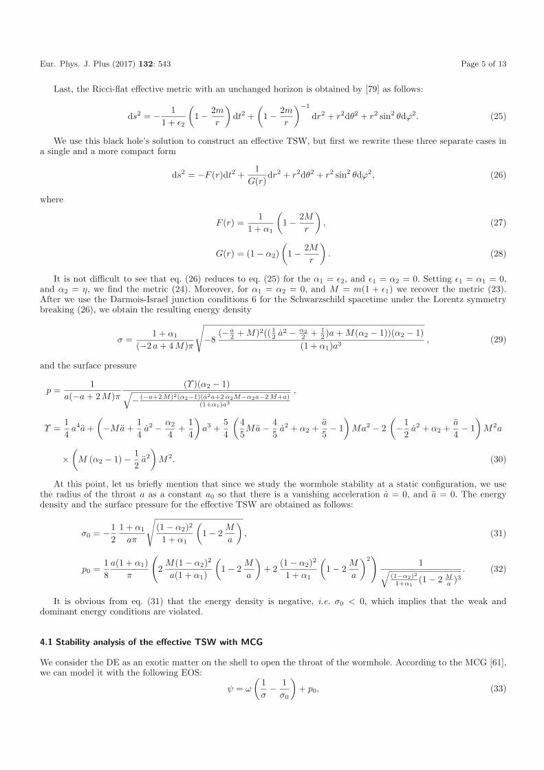
Last, the Ricci-flat effective metric with an unchanged horizon is obtained by [79] as follows:

ds2 = − 11 + ε2

(1 − 2m

r

)dt2 +

(1 − 2m

r

)−1

dr2 + r2dθ2 + r2 sin2 θdϕ2. (25)

We use this black hole’s solution to construct an effective TSW, but first we rewrite these three separate cases ina single and a more compact form

ds2 = −F (r)dt2 +1

G(r)dr2 + r2dθ2 + r2 sin2 θdϕ2, (26)

where

F (r) =1

1 + α1

(1 − 2M

r

), (27)

G(r) = (1 − α2)(

1 − 2M

r

). (28)

It is not difficult to see that eq. (26) reduces to eq. (25) for the α1 = ε2, and ε1 = α2 = 0. Setting ε1 = α1 = 0,and α2 = η, we find the metric (24). Moreover, for α1 = α2 = 0, and M = m(1 + ε1) we recover the metric (23).After we use the Darmois-Israel junction conditions 6 for the Schwarzschild spacetime under the Lorentz symmetrybreaking (26), we obtain the resulting energy density

σ =1 + α1

(−2 a + 4M)π

√−8

(−a2 + M)2((1

2 a2 − α22 + 1

2 )a + M(α2 − 1))(α2 − 1)(1 + α1)a3

, (29)

and the surface pressure

p =1

a(−a + 2M)π(Υ )(α2 − 1)√

− (−a+2 M)2(α2−1)(a2a+2 α2M−α2a−2 M+a)(1+α1)a3

,

Υ =14

a4a +(−Ma +

14

a2 − α2

4+

14

)a3 +

54

(45Ma − 4

5a2 + α2 +

a

5− 1

)Ma2 − 2

(−1

2a2 + α2 +

a

4− 1

)M2a

×(

M (α2 − 1) − 12

a2

)M2. (30)

At this point, let us briefly mention that since we study the wormhole stability at a static configuration, we usethe radius of the throat a as a constant a0 so that there is a vanishing acceleration a = 0, and a = 0. The energydensity and the surface pressure for the effective TSW are obtained as follows:

σ0 = −12

1 + α1

aπ

√(1 − α2)2

1 + α1

(1 − 2

M

a

), (31)

p0 =18

a(1 + α1)π

(2

M(1 − α2)2

a(1 + α1)

(1 − 2

M

a

)+ 2

(1 − α2)2

1 + α1

(1 − 2

M

a

)2)

1√(1−α2)2

1+α1(1 − 2 M

a )3. (32)

It is obvious from eq. (31) that the energy density is negative, i.e. σ0 < 0, which implies that the weak anddominant energy conditions are violated.

4.1 Stability analysis of the effective TSW with MCG

We consider the DE as an exotic matter on the shell to open the throat of the wormhole. According to the MCG [61],we can model it with the following EOS:

ψ = ω

(1σ− 1

σ0

)+ p0, (33)

Page 6 of 13 Eur. Phys. J. Plus (2017) 132: 543

Fig. 2. Here we plot the ω versus a to show stability regions via the MCG.

which is one of the possible candidate for the acceleration of the universe. Then we calculate the derivative of eq. (33)as follows:

ψ′(σ0) = − ω

σ20

. (34)

The second derivative of the potential respect to a is obtained as follows:

V ′′(a) =Θ(a)

(−a + 2M)(−1 + α2)a3(1 + α1), (35)

where

Θ =((−2α1 − 2) α2

2 + (4α1 + 4)α2 − 16π2ω − 2α1 − 2)a6 + 4

((1 + α1) α2

2 + (−2α1 − 2) α2 + 4π2ω + α1 + 1)Ma5

+(−2 (−1 + α2)

2M2 (1 + α1) + (6α1 + 6) α2

2 + (−12α1 − 12) α2 + 32π2ω + 6α1 + 6)

a4

− 18(

(1 + α1) α22 + (−2α1 − 2) α2 +

32π2ω

9+ α1 + 1

)Ma3 + 12 (1 + α1) (−1 + α2)

2

(M2 − 1

2

)a2

+ 20M (−1 + α2)2 (1 + α1) a − 16 (−1 + α2)

2M2 (1 + α1)

and then the ω for the case of V ′′(a0) ≥ 0 is obtained as follows:

ω =18

(α2 − 1)2(a6 − 2Ma5 + (M2 − 3)a4 + 9Ma3 + (−6M2 + 3)a2 − 10Ma + 8M2)(1 + α1)π2a3(Ma2 − a3 − 4M + 2 a)

. (36)

The stability regions of the effective TSW with MCG is shown on plots of ω versus a0 for different values of theparameters ε1, α1 and α2 in figs. 2, 3, 4. Then, we show the effect of α1, α2, ε1 on the second derivative of the potential,where it is stable at V ′′(a0) ≥ 0 and outside the event horizon a > rH , by plotting in figs. 5, 6, 7.

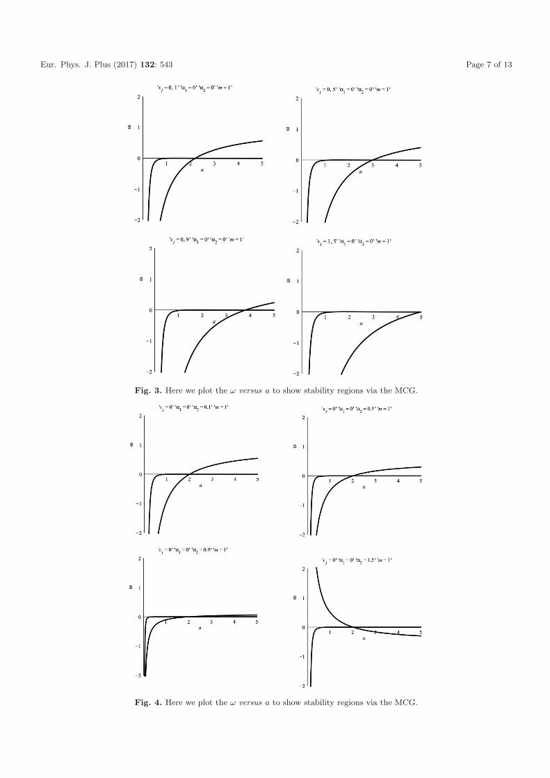
Eur. Phys. J. Plus (2017) 132: 543 Page 7 of 13

Fig. 3. Here we plot the ω versus a to show stability regions via the MCG.

Fig. 4. Here we plot the ω versus a to show stability regions via the MCG.

Page 8 of 13 Eur. Phys. J. Plus (2017) 132: 543

Fig. 5. Here we plot the V ′′ versus a to show stability regions via the MCG.

Fig. 6. Here we plot the V ′′ versus a to show stability regions via the MCG.

Eur. Phys. J. Plus (2017) 132: 543 Page 9 of 13

Fig. 7. Here we plot the V ′′ versus a to show stability regions via the MCG.

4.2 Stability analysis of the effective TSW with a dark sector

Now, we use the EOS of MCG as a unified DE and DM, which is known as a dark sector, can be cast into [36,61,62]

pMCG = BρMCG − A/ραMCG, (37)

where B, A and α are free parameters. From the Friedman-Robertson-Walkers (FRW) universe, using the energyconservation of MCG, one can rewrite the energy density of MCG as follows:

ρMCG = ρMCG0

[Bs + (1 − Bs)a−3(1+B)(1+α)

] 11+α

, (38)

for B �= −1, where Bs = A/(1 + B)ρ1+αMCG0. For the positive energy density, the condition 0 ≤ Bs ≤ 1 is written. The

standard ΛCDM model is recovered when α = 0 and B = 0. For the MCG with dark sector, the Friedmann equationscan be written as follows [36]:

H2 = H20

{Ωa−3 + Ωra

−4 + Ωka−2 + (1 − Ωb − Ωr − Ωk)

×[Bs + (1 − Bs)a−3(1+B)(1+α)

]}. (39)

Note that here H is the Hubble parameter and its current value is H0 = 70h kms−1Mpc−1 [88], and Ωi (i = b, r, k)are dimensionless energy parameters of baryon, radiation and effective curvature density, respectively. Furthermore,when B = 0, the MCG becomes the generalized Chaplygin gas, which is the simplest single dark fluid model (DM +DE). Moreover, if B = 0 and α = 0, it becomes ΛCDM model. In this paper, we consider B �= 0, in which case thesound speed is given by [73,74]

c2s =

dp

dρ= B + α

A

ρα+1. (40)

Page 10 of 13 Eur. Phys. J. Plus (2017) 132: 543

Fig. 8. Here we plot the V ′′ versus a to show stability regions with MCG as DE and DM with β = 1.

It is noted that imaginary part of the sound speeds are related with instabilities especially on very small scales. Herewe consider a model with parameters of range A ≥ 0, B ≥ 0 and 0 ≤ α ≤ 1, with c2

s ≥ 0. It is noted that the valueof c2

s is always larger than or equal to B (for large energy densities). In this limit, the MCG behaves similarly toDM. The constraint obtained using the data of CMB [36]. The ΛCDM model is obtained for small values of α and B.Furthermore, today data is favor of the MCG model.

To check the stability of the effective TSW, we rewrite eq. (37) as follows [36,73,74]:

ψ = βσ0 −(

η

σζ0

), (41)

where B = β, ρMCG = σ0, A = η, α = ζ. The resulting first derivative of function ψ is

ψ′(σ0) = β + ζ

(η

σζ+10

). (42)

Note that β, η and ζ are constant parameters.

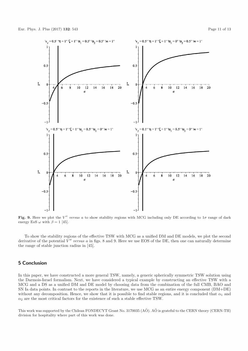
Eur. Phys. J. Plus (2017) 132: 543 Page 11 of 13

Fig. 9. Here we plot the V ′′ versus a to show stability regions with MCG including only DE according to 1σ range of darkenergy EoS ω with β = 1 [45].

To show the stability regions of the effective TSW with MCG as a unified DM and DE models, we plot the secondderivative of the potential V ′′ versus a in figs. 8 and 9. Here we use EOS of the DE, then one can naturally determinethe range of stable junction radius in [45].

5 Conclusion

In this paper, we have constructed a more general TSW, namely, a generic spherically symmetric TSW solution usingthe Darmois-Israel formalism. Next, we have considered a typical example by constructing an effective TSW with aMCG and a DS as a unified DM and DE model by choosing data from the combination of the full CMB, BAO andSN Ia data points. In contrast to the reports in the literature, we use MCG as an entire energy component (DM+DE)without any decomposition. Hence, we show that it is possible to find stable regions, and it is concluded that α1 andα2 are the most critical factors for the existence of such a stable effective TSW.

This work was supported by the Chilean FONDECYT Grant No. 3170035 (AO). AO is grateful to the CERN theory (CERN-TH)division for hospitality where part of this work was done.

Page 12 of 13 Eur. Phys. J. Plus (2017) 132: 543

References

1. M.S. Moris, K.S. Thorne, Am. J. Phys. 56, 395 (1988).2. M. Morris, K.S. Thorne, U. Yurtsever, Phys. Rev. Lett. 61, 1446 (1988).3. M. Visser, Lorentzian Wormholes: From Einstein to Hawking (Springer, Berlin, 1997).4. M. Visser et al., Phys. Rev. Lett. 90, 201102 (2003).5. M. Visser, Nucl. Phys. B 328, 203 (1989).6. M. Visser, Phys. Rev. D 39, 3182 (1989).7. N.M. Garcia, F.S.N. Lobo, M. Visser, Phys. Rev. D 86, 044026 (2012).8. C. Bejarano, E.F. Eiroa, C. Simeone, Eur. Phys. J. C 74, 3015 (2014).9. P. Musgrave, K. Lake, Class. Quantum Grav. 13, 1885 (1996).

10. P. Musgrave, K. Lake, Class. Quantum Grav. 14, 1285 (1997).11. M. Ishak, K. Lake, Phys. Rev. D 65, 044011 (2002).12. E.F. Eiroa, Phys. Rev. D 78, 024018 (2008).13. M. Halilsoy, A. Ovgun, S. Habib Mazharimousavi, Eur. Phys. J. C 74, 2796 (2014).14. K. Jusufi, A. Ovgun, Mod. Phys. Lett. A 32, 1750047 (2017).15. F. Rahaman, M. Kalam, S. Chakraborty, Gen. Relativ. Gravit. 38, 1687 (2006).16. A. Ovgun, Eur. Phys. J. Plus 131, 389 (2016).17. Kimet Jusufi, Eur. Phys. J. C 76, 608 (2016).18. A. Ovgun, K. Jusufi, Adv. High Energy Phys. 2017, 1215254 (2017).19. A. Ovgun, I. Sakalli, I. Theor. Math. Phys. 190, 120 (2017).20. M.G. Richarte, I.G. Salako, J.P. Morais Graca, H. Moradpour, Ali Ovgun, Phys. Rev. D 96, 084022 (2017).21. P. Bhar, A. Banerjee, Int. J. Mod. Phys. D 24, 1550034 (2015).22. M. Sharif, M. Azam, JCAP 04, 023 (2013).23. M. Sharif, M. Azam, Eur. Phys. J. C 73, 2407 (2013).24. M. Sharif, F. Javed, Gen. Relativ. Gravit. 48, 158 (2016).25. M. Sharif, S. Mumtaz, Astrophys. Space Sci. 361, 218 (2016).26. V. Varela, Phys. Rev. D 92, 044002 (2015).27. P.K.F. Kuhfittig, Ann. Phys. 355, 115 (2015).28. M. Azam, Astrophys. Space Sci. 361, 96 (2016).29. M. Jamil, Peter K.F. Kuhfittig, F. Rahaman, Sk.A. Rakib, Eur. Phys. J. C 67, 513 (2010).30. M. Sharif, S. Mumtaz, Adv. High Energy Phys. 2016, 2868750 (2016).31. A. Banerjee, Int. J. Theor. Phys. 52, 2943 (2013).32. A. Ovgun, I.G. Salako, Mod. Phys. Lett. A 32, 1750119 (2017).33. A. Ovgun, A. Banerjee, K. Jusufi, Eur. Phys. J. C 77, 566 (2017).34. D. Wang, X. Meng, Eur. Phys. J. C 76, 171 (2016).35. D. Wang, X. Meng, Eur. Phys. J. C 76, 484 (2016).36. L. Xu, Y. Wang, H. Noh, Eur. Phys. J. C 72, 1931 (2012).37. K. Jusufi, A. Ovgun, Astrophys. Space Sci. 361, 207 (2016).38. A. Eid, J. Korean, Phys. Soc. 70, 436 (2017).39. S. Chakraborty, Gen. Relativ. Gravit. 49, 47 (2017).40. A. Banerjee, K. Jusufi, S. Bahamonde, arXiv:1612.06892.41. A. Eid, Eur. Phys. J. Plus 131, 23 (2016).42. F.S.N. Lobo, M. Bouhmadi-Lopez, P. Martin-Moruno, N. Montelongo-Garcia, M. Visser, arXiv:1512.08474.43. E.F. Eiroa, G.F. Aguirre, Eur. Phys. J. C 76, 132 (2016).44. M. Sharif, S. Mumtaz, Can. J. Phys. 94, 158 (2016).45. D. Wang, X. Meng, Phys. Dark Univ. 17, 46 (2017).46. J.P.M. Pitelli, R.A. Mosna, Phys. Rev. D 91, 124025 (2015).47. D. Wang, X.H. Meng, Front. Phys. (Beijing) 13, 139801 (2018).48. D. Wang, X.H. Meng, Phys. Dark Univ. 16, 81 (2017).49. M.G. Richarte, Phys. Rev. D 87, 067503 (2013).50. M. Zaeem-ul-Haq Bhatti, Z. Yousaf, S. Ashraf, Ann. Phys. 383, 439 (2017).51. M.Z.u.H. Bhatti, A. Anwar, S. Ashraf, Mod. Phys. Lett. A 32, 1750111 (2017).52. E. Guendelman, E. Nissimov, S. Pacheva, M. Stoilov, Bulg. J. Phys. 44, 85 (2017).53. E. Guendelman, E. Nissimov, S. Pacheva, M. Stoilov, Springer Proc. Math. Stat. 191, 245 (2016).54. N. Sen, Ann. Phys. (Leipzig) 73, 365 (1924).55. K. Lanczos, Ann. Phys. (Leipzig) 74, 518 (1924).56. G. Darmois, Memorial des Sciences Mathematique, Vol. 25 (Gauthier-Villars, 1927).57. Israel, Nuovo Cimento B 44, 1 (1966).58. E.I. Guendelman, I. Shilon, Class. Quantum Grav. 26, 045007 (2009).59. A. Kamenshchik, U. Moschella, V. Pasquier, Phys. Lett. B 511, 265 (2001).60. M.C. Bento, O. Bertolami, A.A. Sen, Phys. Rev. D 66, 043507 (2002).61. J.D. Barrow, Nucl. Phys. B 310, 743 (1988).

Eur. Phys. J. Plus (2017) 132: 543 Page 13 of 13

62. J. Lu, L. Xu, Y. Wu, M. Liu, Gen. Relativ. Gravit. 43, 819 (2011).63. N. Suzuki, D. Rubin, C. Lidman, G. Aldering, R. Amanullah et al., Astrophys. J. 746, 85 (2012).64. L. Anderson, E. Aubourg, S. Bailey, D. Bizyaev, M. Blanton et al., Mon. Not. R. Astron. Soc. 427, 3435 (2013).65. D. Parkinson, S. Riemer-Sorensen, C. Blake, G.B. Poole, T.M. Davis et al., Phys. Rev. D 86, 103518 (2012).66. WMAP Collaboration (G. Hinshaw et al.), Astrophys. J. Suppl. 208, 19 (2013).67. Planck Collaboration (P.A.R. Ade et al.), Astron. Astrophys. 571, A16 (2014).68. Planck Collaboration (P.A.R. Ade et al.), arXiv:1502.01589 (2015).69. A. Ovgun, G. Leon, J. Magana, K. Jusufi, arXiv:1709.09794 [gr-qc].70. A. Ovgun, Eur. Phys. J. C 77, 105 (2017).71. J. Frieman, M. Turner, D. Huterer, Annu. Rev. Astron. Astrophys. 46, 385 (2008).72. N. Kaloper, A. Padilla, Phys. Rev. Lett. 112, 091304 (2014).73. P.P. Avelino, V.M.C. Ferreira, Phys. Rev. D 91, 083508 (2015).74. P.P. Avelino, L.M.G. Beca, J.P.M. de Carvalho, C.J.A.P. Martins, JCAP 09, 002 (2003).75. M.C. Bento, O. Bertolami, A.A. Sen, Phys. Rev. D 66, 043507 (2002).76. N. Bilic, G.B. Tupper, R.D. Viollier, Phys. Lett. B 535, 17 (2002).77. V. Gorini, A. Kamenshchik, U. Moschella, Phys. Rev. D 67, 063509 (2003).78. J. Lu, L. Xu, J. Li, B. Chang, Y. Gui, H. Liu, Phys. Lett. B 662, 87 (2008).79. G. Betschart, E. Kant, F.R. Klinkhamer, Nucl. Phys. B 815, 198 (2009).80. C. Hoffmann, T. Ioannidou, S. Kahlen, B. Kleihaus, J. Kunz, Phys. Rev. D 95, 084010 (2017).81. H. Belich, C. Furtado, K. Bakke, Eur. Phys. J. C 75, 410 (2015).82. K. Bakke, H. Belich, J. Phys. G: Nucl. Part. Phys. 42, 095001 (2015).83. K. Bakke, H. Belich, Ann. Phys. (NY) 354, 1 (2015).84. H. Belich, K. Bakke, Phys. Rev. D 90, 025026 (2014).85. A.G. de Lima, H. Belich, K. Bakke, Rev. Math. Phys. 28, 1650023 (2016).86. H.F. Mota, K. Bakke, Phys. Rev. D 89, 027702 (2014).87. H. Belich, K. Bakke, Int. J. Mod. Phys. A 31, 1650026 (2016).88. LIGO Scientific and Virgo and 1M2H and DLT40 and Las Cumbres Observatory and VINROUGE and MASTER Collab-

orations (B.P. Abbott et al.), Nature https://doi.org/10.1038/nature24471 (arXiv:1710.05835 [astro-ph.CO]).