Stability of discrete solitons in nonlinear Schrodinger...
19
Physica D 212 (2005) 1–19 www.elsevier.com/locate/physd Stability of discrete solitons in nonlinear Schr ¨ odinger lattices D.E. Pelinovsky a , P.G. Kevrekidis b,* , D.J. Frantzeskakis c a Department of Mathematics, McMaster University, Hamilton, Ontario, Canada L8S 4K1 b Department of Mathematics, University of Massachusetts, Amherst, MA, 01003-4515, USA c Department of Physics, University of Athens, Panepistimiopolis, Zografos, Athens 15784, Greece Received 11 August 2004; received in revised form 24 January 2005; accepted 11 July 2005 Available online 2 November 2005 Communicated by C.K.R.T. Jones Abstract We consider the discrete solitons bifurcating from the anti-continuum limit of the discrete nonlinear Schr¨ odinger (NLS) lattice. The discrete soliton in the anti-continuum limit represents an arbitrary finite superposition of in-phase or anti-phase excited nodes, separated by an arbitrary sequence of empty nodes. By using stability analysis, we prove that the discrete solitons are all unstable near the anti-continuum limit, except for the solitons, which consist of alternating anti-phase excited nodes. We classify analytically and confirm numerically the number of unstable eigenvalues associated with each family of the discrete solitons. c 2005 Elsevier B.V. All rights reserved. Keywords: Discrete nonlinear Schr ¨ odinger equation; Discrete solitons; Existence and stability; Lyapunov–Schmidt reductions 1. Introduction Nonlinear instabilities and the emergence of coherent structures in differential–difference equations have become topics of physical importance and mathematical interest in the past decade. Numerous applications of these problems have emerged ranging from nonlinear optics, in the dynamics of guided waves in inhomogeneous optical structures [1,2] and photonic crystal lattices [3,4], to atomic physics, in the dynamics of Bose–Einstein condensate droplets in periodic (optical lattice) potentials [5–8] and from condensed matter, in Josephson-junction ladders [9,10], to biophysics, in various models of the DNA double strand [11,12]. This large range of models and applications has been summarized in a variety of reviews such as [13–17]. * Corresponding author. E-mail address: [email protected] (P.G. Kevrekidis). 0167-2789/$ - see front matter c 2005 Elsevier B.V. All rights reserved. doi:10.1016/j.physd.2005.07.021
Transcript of Stability of discrete solitons in nonlinear Schrodinger...
Physica D 212 (2005) 1–19www.elsevier.com/locate/physd
Stability of discrete solitons in nonlinear Schrodinger lattices
D.E. Pelinovskya, P.G. Kevrekidisb,∗, D.J. Frantzeskakisc
a Department of Mathematics, McMaster University, Hamilton, Ontario, Canada L8S 4K1b Department of Mathematics, University of Massachusetts, Amherst, MA, 01003-4515, USA
c Department of Physics, University of Athens, Panepistimiopolis, Zografos, Athens 15784, Greece
Received 11 August 2004; received in revised form 24 January 2005; accepted 11 July 2005Available online 2 November 2005Communicated by C.K.R.T. Jones
Abstract
We consider the discrete solitons bifurcating from the anti-continuum limit of the discrete nonlinear Schrodinger (NLS)lattice. The discrete soliton in the anti-continuum limit represents an arbitrary finite superposition of in-phase or anti-phaseexcited nodes, separated by an arbitrary sequence of empty nodes. By using stability analysis, we prove that the discrete solitonsare all unstable near the anti-continuum limit, except for the solitons, which consist of alternating anti-phase excited nodes. Weclassify analytically and confirm numerically the number of unstable eigenvalues associated with each family of the discretesolitons.c© 2005 Elsevier B.V. All rights reserved.
Keywords: Discrete nonlinear Schrodinger equation; Discrete solitons; Existence and stability; Lyapunov–Schmidt reductions
1. Introduction
Nonlinear instabilities and the emergence of coherent structures in differential–difference equations havebecome topics of physical importance and mathematical interest in the past decade. Numerous applications ofthese problems have emerged ranging from nonlinear optics, in the dynamics of guided waves in inhomogeneousoptical structures [1,2] and photonic crystal lattices [3,4], to atomic physics, in the dynamics of Bose–Einsteincondensate droplets in periodic (optical lattice) potentials [5–8] and from condensed matter, in Josephson-junctionladders [9,10], to biophysics, in various models of the DNA double strand [11,12]. This large range of models andapplications has been summarized in a variety of reviews such as [13–17].
∗ Corresponding author.E-mail address: [email protected] (P.G. Kevrekidis).
0167-2789/$ - see front matter c© 2005 Elsevier B.V. All rights reserved.doi:10.1016/j.physd.2005.07.021

2 D.E. Pelinovsky et al. / Physica D 212 (2005) 1–19
One of the prototypical differential–difference models that is both physically relevant and mathematicallytractable is the so-called discrete nonlinear Schrodinger (NLS) equation,
iun + ε∆dun + γ |un|2un = 0, (1.1)
where un = un(t) is a complex amplitude in time t , n ∈ Zd is the d-dimensional lattice, ∆d is the d-dimensionaldiscrete Laplacian (the “standard” one constructed out of three-point stencils in each lattice direction), ε is thedispersion coefficient, and γ is the nonlinearity coefficient. Before we delve into mathematical analysis of thediscrete NLS equation, it is relevant to discuss briefly the recent physical applications of this model.
The most direct implementation of the discrete NLS-type equations can be identified in one-dimensional arraysof coupled optical waveguides [1,2]. These may be multi-core structures created in a slab of a semiconductormaterial (such as AlGaAs), or virtual ones, induced by a set of laser beams illuminating a photorefractive crystal.In this experimental implementation, there are about forty lattice sites (guiding cores), and the localized modes(discrete solitons) may propagate over many diffraction lengths.
Light-induced photonic lattices [3,4] have recently emerged as an important application of such equations. Therefractive index of the nonlinear photonic lattices changes periodically due to a grid of strong beams, while a weakerprobe beam is used to monitor the localized modes (discrete solitons). A number of promising experimental studiesof discrete solitons in light-induced photonic lattices were reported recently in the physics literature.
An array of Bose–Einstein condensate droplets trapped in a strong optical lattice with thousands of atoms ineach droplet is another direct physical realization of the discrete NLS equation [5,6]. In this context, the model canbe derived systematically by using the Wannier function expansions [7,8].
Besides applications to optical waveguides, photonic crystal lattices, and Bose–Einstein condensates trappedin optical lattices, the discrete NLS equation also arises as the envelope wave reduction of the general nonlinearKlein–Gordon lattices [18].
This rich variety of physical contexts makes it timely and relevant to analyze the mathematical aspects of thediscrete NLS equation (1.1), including the existence and stability of localized modes (discrete solitons). A veryhelpful tool for such an analysis is the so-called anti-continuum limit ε → 0 [13], where the nonlinear oscillatorsof the model are uncoupled. The existence of localized modes in this limit can be characterized in full detail [15].The persistence, multiplicity, and stability of localized modes can be studied with continuation methods bothanalytically and numerically [19].
Our aim is to study localized modes of the discrete NLS equation (1.1) in two papers. The present paperdescribes the stability analysis of discrete solitons in the one-dimensional NLS lattice (d = 1). A separate workwill present Lyapunov–Schmidt reductions for the persistence, multiplicity and stability of discrete vortices in thetwo-dimensional NLS lattice (d = 2).
This paper is structured as follows. We review the known results on the existence of one-dimensional discretesolitons in Section 2. General stability and instability results for discrete solitons in the anti-continuum limit areproved in Section 3. These stability results are illustrated for two particular families of the discrete solitons inSections 4 and 5. Besides explicit perturbation series expansion results, we compare asymptotic approximations andnumerical computations of stable and unstable eigenvalues in the linearized stability problem. Section 6 containsour conclusions.
2. Existence of discrete solitons
We consider the normalized form of the discrete NLS equation (1.1) in one dimension (d = 1):
iun + ε(un+1 − 2un + un−1) + |un|2un = 0, (2.1)
where un(t) : R+ → C, n ∈ Z, and ε > 0 is the inverse squared step size of the discrete one-dimensional NLSlattice. The discrete solitons are given by the time-periodic solutions of the discrete NLS equation (2.1):
D.E. Pelinovsky et al. / Physica D 212 (2005) 1–19 3
un(t) = φnei(µ−2ε)t+iθ0 , µ ∈ R, φn ∈ C, n ∈ Z, (2.2)
where θ0 ∈ R is a parameter and (µ, φn) solve the nonlinear difference equations on n ∈ Z:
(µ − |φn|2)φn = ε(φn+1 + φn−1). (2.3)
The existence of the discrete solitons was studied recently in [20–22], inspired by the pioneer papers [23,24]. Arecent summary of the existence results is given in [19]. Since discrete solitons in the focusing NLS lattice (2.1)only exist for µ > 2ε [19] and the parameter µ is scaled out by the scaling transformation
φn =√
µφn, ε = µε, (2.4)
the parameter µ will henceforth be set as µ = 1. Another arbitrary parameter θ0, which exists due to the gaugeinvariance of the discrete NLS equation (2.1), is incorporated in the ansatz (2.2) such that at least one value ofφn can be chosen real valued without lack of generality. Using this convention, we represent below the knownexistence results.
Proposition 2.1. There exist ε0 > 0, κ > 0 and φ∞ > 0 such that the difference equations (2.3) with µ = 1 and0 < ε < ε0 have continuous families of discrete solitons with the properties:
(i)
limε→0+
φn = φ(0)n =
eiθn , n ∈ S,
0, n ∈ Z \ S,(2.5)
(ii)
lim|n|→∞
eκ|n||φn| = φ∞, (2.6)
(iii)
φn ∈ R, n ∈ Z, (2.7)
where S is a finite set of nodes of the lattice n ∈ Z and θn = 0, π, n ∈ S.
Proof. See Theorem 2.1 and Appendices A and B in [19] for the proof of the limiting solution (2.5) from theinverse function theorem. See Theorem 3 in [24] for the proof of the exponential decay (2.6) from the boundestimates. See Section 3.2 in [15] for the proof of the reality condition (2.7) from the conservation of the densitycurrent. Various theoretical and numerical bounds on ε0 are obtained in [15,19,20,24].
Due to the property (2.7), the difference equations (2.3) with µ = 1 can be rewritten as follows:
(1 − φ2n)φn = ε(φn+1 + φn−1), n ∈ Z. (2.8)
For our analysis, we shall derive two technical results on properties of solutions φn , n ∈ Z.
Lemma 2.2. There exists ε0 > 0 such that the solution φn , n ∈ Z, is represented by the convergent power seriesfor 0 ≤ ε < ε0:
φn = φ(0)n +
∞∑k=1
εkφ(k)n , (2.9)
where φ(0)n is given by (2.5).
Proof. The statement follows from the Implicit Function Theorem (see Theorem 2.7.2 in [25]), since the Jacobianmatrix for the system (2.8) is non-singular at φn = φ
(0)n , n ∈ Z, while the right-hand side of the system (2.8) is
analytic in ε.
4 D.E. Pelinovsky et al. / Physica D 212 (2005) 1–19
Lemma 2.3. There exists 0 < ε1 < ε0 such that the number of changes in the sign of φn on n ∈ Z for 0 < ε < ε1is equal to the number of π-differences of the adjacent θn, n ∈ S, in the limiting solution (2.5).
Proof. Consider two adjacent excited nodes n1, n2 ∈ S separated by N empty nodes such that n2 − n1 = 1 + Nand N ≥ 1. We need to prove that the number of π -differences in the argument of φn , n1 ≤ n ≤ n2, for smallε > 0 is exactly one if θn2 − θn1 = π and zero if θn2 − θn1 = 0. To do so, we consider the difference equations(2.8) on n1 < n < n2 as the N -by-N matrix system
ANφN = εbN , (2.10)
where φN = (φn1+1, . . . , φn2−1)T, and
AN =
1 − φ2
n1+1 −ε 0 · · · 0−ε 1 − φ2
n1+2 −ε · · · 0...
...... · · ·
...
0 0 0 · · · 1 − φ2n2−1
, bN =
φn1
0...
φn2
. (2.11)
Let DI,J , 1 ≤ I ≤ J ≤ N , be the determinant of the block of the matrix AN between the I -th and J -th rows andcolumns. By Cramer’s rule, we have
φn1+ j =ε jφn1 D j+1,N + εN− j+1φn2 D1,N− j
D1,N. (2.12)
Since limε→0 DI,J = 1 for all 1 ≤ I ≤ J ≤ N , we have
limε→0
ε− jφn1+ j = φn1 , 1 ≤ j <N + 1
2,
limε→0
ε− jφn1+ j = φn1 + φn2 , j =N + 1
2,
limε→0
ε j−1−N φn1+ j = φn2 ,N + 1
2< j ≤ N .
The statement of Lemma follows from the signs of φn , n1 ≤ n ≤ n2, for small ε > 0.
By Proposition 2.1 and Lemma 2.3, all families of the discrete solitons as ε → 0 can be classified by a sequenceof 0, +, and − of the limiting solution (2.5) on the finite set S [19]. In particular, we consider two orderedsets S:
S1 = 1, 2, 3, . . . , N (2.13)
and
S2 = 1, 3, 5, . . . , 2N − 1, (2.14)
where dim(S1) = dim(S2) = N < ∞. The set S1 includes the Page mode (N = 2: θ1 = θ2 = 0) and the twistedmode (N = 2: θ1 = 0, θ2 = π ). The set S2 includes the Page and twisted modes (N = 2), separated by an emptynode.
3. Stability of discrete solitons
The spectral stability of discrete solitons is studied with the standard linearization
un(t) = ei(1−2ε)t+iθ0(φn + aneλt+ bneλt ), λ ∈ C, (an, bn) ∈ C2, n ∈ Z, (3.1)
where (λ, an, bn) solve the linear eigenvalue problem on n ∈ Z:
D.E. Pelinovsky et al. / Physica D 212 (2005) 1–19 5
(1 − 2φ2n)an − φ2
nbn − ε(an+1 + an−1) = iλan,
−φ2nan + (1 − 2φ2
n)bn − ε(bn+1 + bn−1) = −iλbn .(3.2)
The discrete soliton (2.2) is called spectrally unstable if there exist λ and (an, bn), n ∈ Z, in the problem (3.2)such that Re(λ) > 0 and
∑n∈Z(|an|
2+ |bn|
2) < ∞. Otherwise, the soliton is called weakly spectrally stable.Orbital stability of the discrete one-pulse soliton was studied in the anti-continuum limit ε → 0 [26] and closeto the continuum limit ε → ∞ [27]. Spectral instabilities of two-pulse and multi-pulse solitons were consideredin [28–33] using numerical and variational approximations. It was well understood from intuition supported bynumerical simulations [13,32] that the discrete solitons with the alternating sequence of θn = 0, π in the limitingsolution (2.5) are spectrally stable as ε → 0 but have eigenvalues with so-called negative Krein signature, whichbecome complex by means of the Hamiltonian–Hopf bifurcations [29,33]. All other families of discrete solitonshave unstable real eigenvalues λ in the anti-continuum limit for any ε 6= 0 [32].
Here we prove these preliminary observations and find the precise number of stable and unstable eigenvaluesin the linearized stability problem (3.2) for small ε > 0. Our results are similar to those in the Lyapunov–Schmidtreductions, which are applied to continuous multi-pulse solitons in nonlinear Schrodinger equations [34–37]. Inparticular, the main conclusion on stability of alternating up–down solitons and instability of any other up–up anddown–down sequences of solitons was found for multi-pulse homoclinic orbits arising in the so-called orbit-flipbifurcation [34, p. 176]. The same conclusion agrees with qualitative predictions for the discrete NLS equations [32,p. 66].
Let Ω = l2(Z, C) be the Hilbert space of square-summable bi-infinite complex-valued sequences unn∈Z,equipped with the inner product and norm
(u, w)Ω =
∑n∈Z
unwn, ‖u‖2Ω =
∑n∈Z
|un|2 < ∞. (3.3)
We use bold notation u for an infinite-dimensional vector in Ω that consists of components un for all n ∈ Z. Thestability problem (3.2) is transformed with the substitution
an = un + iwn, bn = un − iwn, n ∈ Z, (3.4)
to the form
(1 − 3φ2n)un − ε(un+1 + un−1) = −λwn,
(1 − φ2n)wn − ε(wn+1 + wn−1) = λun .
(3.5)
The matrix–vector form of the problem (3.5) is
L+u = −λw, L−w = λu, (3.6)
where L± are infinite-dimensional symmetric tri-diagonal matrices, which consist of the elements
(L+)n,n = 1 − 3φ2n , (L−)n,n = 1 − φ2
n , (L±)n,n+1 = (L±)n+1,n = −ε.
Equivalently, the stability problem (3.6) is rewritten in the Hamiltonian form
JHψ = λψ, (3.7)
where ψ is the infinite-dimensional eigenvector, which consists of 2-blocks of (un, wn)T , J is the infinite-dimensional skew-symmetric matrix, which consists of 2-by-2 blocks of
Jn,m =
(0 1
−1 0
)δn,m,
6 D.E. Pelinovsky et al. / Physica D 212 (2005) 1–19
andH is the infinite-dimensional symmetric matrix, which consists of 2-by-2 blocks of
Hn,m =
((L+)n,m 0
0 (L−)n,m
).
The representation (3.7) follows from the Hamiltonian structure of the discrete NLS equation (2.1), where J is thesymplectic operator andH is the linearized Hamiltonian. By Lemma 2.2, the matrixH is expanded into the powerseries
H = H(0)+
∞∑k=1
εkH(k), (3.8)
whereH(0) is diagonal with two blocks:
H(0)n,n =
(−2 00 0
), n ∈ S, H(0)
n,n =
(1 00 1
), n ∈ Z \ S. (3.9)
Let N = dim(S) < ∞. The spectrum of H(0)ϕ = γϕ has exactly N negative eigenvalues γ = −2, N zeroeigenvalues γ = 0 and infinitely many positive eigenvalues γ = +1. The negative and zero eigenvalues γ = −2and γ = 0 map to N double zero eigenvalues λ = 0 in the eigenvalue problem JH(0)ψ = λψ . The positiveeigenvalues γ = +1 map to the infinitely many eigenvalues λ = ±i.
Since finitely many zero eigenvalues of JH(0) are isolated from the rest of the spectrum, their shifts vanishas ε → 0, according to the regular perturbation theory [38]. We can therefore locate small unstable eigenvaluesRe(λ) > 0 of the stability problem (3.7) for small ε > 0 from their limits at ε = 0. On the other hand, infinitelymany imaginary eigenvalues of JH(0) become the continuous spectrum band as ε 6= 0 [39]. However, since thedifference operator JH has exponentially decaying potentials φn , n ∈ Z, due to the decay condition (2.6), thecontinuous spectral bands of JH are located on the imaginary axis of λ near the points λ = ±i, similarly tothe case for φn = 0, n ∈ Z [39]. Therefore, the infinite-dimensional part of the spectrum does not produce anyunstable eigenvalues Re(λ) > 0 in the stability problem (3.7) as ε > 0. Results of the regular perturbation theoryare formulated and proved below.
Lemma 3.1. Assume that φn , n ∈ Z, is the discrete soliton, described in Proposition 2.1. Let N = dim(S) < ∞.Let γ j , 1 ≤ j ≤ N be small eigenvalues of H as ε → 0 such that
limε→0
γ j = 0, 1 ≤ j ≤ N . (3.10)
There exists 0 < ε∗ ≤ ε0 such that the eigenvalue problem (3.7) with φn , n ∈ Z, and 0 < ε < ε∗ has N pairs ofsmall eigenvalues λ j and −λ j , 1 ≤ j ≤ N, that satisfy the leading-order behavior
limε→0
λ2j
γ j= 2, 1 ≤ j ≤ N . (3.11)
Proof. Since the operator L+ is Fredholm of zero index and empty kernel at ε = 0, it can be inverted for smallε > 0 and the non-self-adjoint eigenvalue problem (3.6) can be transformed to the self-adjoint diagonalizationproblem
L−w = −λ2L−1+ w, (3.12)
such that
λ2= −
(w,L−w)Ω
(w,L−1+ w)Ω
, (3.13)
D.E. Pelinovsky et al. / Physica D 212 (2005) 1–19 7
where the inner product is defined in (3.3). Since all small eigenvalues of H are small eigenvalues of L−, wedenote by w j an eigenvector of L− which corresponds to the small eigenvalue γ j , 1 ≤ j ≤ N , in the limiting
condition (3.10). By continuity of the eigenvectors and completeness of ker(L(0)− ), there exists a set of normalized
coefficients cn, j n∈S for each 1 ≤ j ≤ N such that
limε→0
w j = w(0)j =
∑n∈S
cn, j en,∑n∈S
|cn, j |2
= 1, (3.14)
where en is the unit vector in Ω . It follows from the direct computations that
limε→0
(w j ,L−1+ w j ) = (w(0)
j ,L(0)−1+ w(0)
j ) = −12. (3.15)
The leading-order behavior (3.11) follows from (3.13) and (3.15) by the regular perturbation theory [38].
Corollary 3.2. Each small positive eigenvalue γ j corresponds to a pair of positive and negative eigenvalues λ jand −λ j for small ε > 0. Each small negative eigenvalue γ j corresponds to a pair of purely imaginary eigenvaluesλ j and −λ j for small ε > 0. The latter eigenvalues have negative Krein signature:
(ψ,Hψ) = (u,L+u) + (w,L−w) = 2(w,L−w) < 0. (3.16)
For any ε 6= 0, there exists a simple zero eigenvalue of H due to the gauge symmetry of the discrete solitons(2.2), as the parameter θ0 is arbitrary, such that L−φ = 0. When all other (N − 1) eigenvalues γ j are non-zero forany ε 6= 0, the splitting of the semi-simple zero eigenvalue of H(0) is called generic. The generic splitting gives asufficient condition for unique (up to the gauge invariance) continuation of discrete solitons for ε 6= 0 [34], whichis also guaranteed by Proposition 2.1 [24].
Let n0 and p0 be the numbers of negative and positive eigenvalues γ j , defined in Lemma 3.1. The splitting isgeneric if p0 = N − 1 − n0. The numbers n0 and p0 are computed exactly from the limiting solution (2.5) asfollows.
Lemma 3.3. There exists 0 < ε1 < ε0 such that the index n0 for 0 < ε < ε1 equals the number of π -differencesof the adjacent θn , n ∈ S, in the limiting solution (2.5), while p0 = N − 1 − n0.
Proof. Since L−φ = 0 for any 0 < ε < ε0, the number n0 of negative eigenvalues of L− coincides with thenumber of times when φ changes sign, by the Discrete Sturm–Liouville Theorem [39]. In the case ε = 0, thisnumber equals the number of π -differences of the adjacent θn , n ∈ S, in the limiting solution (2.5). By Lemma 2.3,the number remains continuous as ε 6= 0. The difference equation L−w = 0 has only two fundamental solutionssuch that w = c1w1 + c2w2, where c1, c2 are arbitrary parameters, w1 = φ is exponentially decaying as |n| → ∞,and w2 is exponentially growing as |n| → ∞, due to the discrete Wronskian identity [39]. As a result, the kernelof L− is one-dimensional for ε 6= 0, such that p0 = N − 1 − n0.
It was recently studied [40,41] that there exists a closure relation between the negative index of the linearizedHamiltonianH and the number of unstable eigenvalues of the linearized operator JH. The closure relation can beextended from the coupled NLS equations to the discrete NLS equations by using the same methods [40,41]. Wehence formulate the closure relation for the discrete NLS equations (2.1).
Proposition 3.4. Let n(H) be the finite number of negative eigenvalues of H. Let Nreal be the number of positivereal eigenvalues λ in the problem (3.7), N−
imag be the number of pairs of purely imaginary eigenvalues λ withnegative Krein signature (ψ,Hψ) < 0, and Ncomp be the number of complex eigenvalues λ in the first openquadrant of λ. Let p(P ′) = 1 if P ′
≥ 0 and p(P ′) = 0 if P ′ < 0, where
P ′= ‖φ‖
2Ω − ε
ddε
‖φ‖2Ω . (3.17)
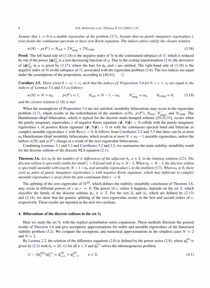
8 D.E. Pelinovsky et al. / Physica D 212 (2005) 1–19
Assume that λ = 0 is a double eigenvalue of the problem (3.7). Assume that no purely imaginary eigenvalues λ
exist inside the continuous spectrum or have zero Krein signature. The indices above satisfy the closure relation
n(H) − p(P ′) = Nreal + 2N−
imag + 2Ncomp. (3.18)
Proof. The left-hand side of (3.18) is the negative index of H in the constrained subspace of Ω , which is reducedby one if the power ‖φ‖
2Ω is a non-decreasing function of µ. Due to the scaling transformation (2.4), the derivative
of ‖φ‖2Ω in µ is given by (3.17), where the hats for φn and ε are omitted. The right-hand side of (3.18) is the
negative index ofH on the subspace of Ω , associated with the eigenvalue problem (3.6). The two indices are equalunder the assumptions of the proposition, according to [40,41].
Corollary 3.5. There exists 0 < ε2 < ε1 such that the indices of Proposition 3.4 for 0 < ε < ε2 are equal to theindices of Lemmas 3.1 and 3.3 as follows:
n(H) = N + n0, p(P ′) = 1, Nreal = N − 1 − n0, N−
imag = n0, Ncomp = 0, (3.19)
and the closure relation (3.18) is met.
When the assumptions of Proposition 3.4 are not satisfied, instability bifurcations may occur in the eigenvalueproblem (3.7), which results in the redistribution of the numbers n(H), p(P ′), Nreal, N−
imag, and Ncomp. TheHamiltonian–Hopf bifurcation, which is typical for the discrete multi-humped solitons [29,31,33], occurs whenthe purely imaginary eigenvalues λ of negative Krein signature (ψ,Hψ) < 0 collide with the purely imaginaryeigenvalues λ of positive Krein signature (ψ,Hψ) > 0 or with the continuous spectral band and bifurcate ascomplex unstable eigenvalues λ with Re(λ) > 0. It follows from Corollaries 3.2 and 3.5 that there can be at mostn0 Hamiltonian–Hopf instability bifurcations, which result in at most N + n0 − 1 unstable eigenvalues, unless theindices n(H) and p(P ′) change as a result of the zero-eigenvalue bifurcations.
Combining Lemmas 3.1 and 3.3 and Corollaries 3.2 and 3.5, we summarize the main stability–instability resultfor the discrete solitons of the discrete NLS equation (2.1).
Theorem 3.6. Let n0 be the number of π -differences of the adjacent θn , n ∈ S, in the limiting solution (2.5). Thediscrete soliton is spectrally stable for small ε > 0 if and only if n0 = N −1. When n0 < N −1, the discrete solitonis spectrally unstable with exactly N −1−n0 real unstable eigenvalues λ in the problem (3.7). When n0 6= 0, thereexist n0 pairs of purely imaginary eigenvalues λ with negative Krein signature, which may bifurcate to complexunstable eigenvalues λ away from the anti-continuum limit ε → 0.
The splitting of the zero eigenvalue of H(0), which defines the stability–instability conclusion of Theorem 3.6,may occur in different powers of ε as ε → 0. The power of ε, where it happens, depends on the set S, whichclassifies the family of the discrete solitons φn , n ∈ Z. For the sets S1 and S2, which are defined by (2.13)and (2.14), we show that the generic splitting of the zero eigenvalue occurs in the first and second orders of ε,respectively. These results are reported in the next two sections.
4. Bifurcations of the discrete solitons in the set S1
Here we study the set S1 with the explicit perturbation series expansions. These methods illustrate the generalresults of Theorem 3.6 and give asymptotic approximations for stable and unstable eigenvalues of the linearizedstability problem (3.2). We compare the asymptotic and numerical approximations in the simplest cases N = 2and N = 3.
By Lemma 2.2, the solution of the difference equations (2.8) is defined by the power series (2.9), where φ(0)n is
given by (2.5) with θn = 0, π for all n ∈ S and φ(1)n solves the inhomogeneous problem
(1 − 3φ(0)2n )φ(1)
n = φ(0)n+1 + φ
(0)n−1, n ∈ Z. (4.1)
D.E. Pelinovsky et al. / Physica D 212 (2005) 1–19 9
For the set S1, defined by (2.13), the system (4.1) has the unique solution
φ(1)n = −
12(cos(θn−1 − θn) + cos(θn+1 − θn))eiθn , 2 ≤ n ≤ N − 1,
φ(1)1 = −
12
cos(θ2 − θ1)eiθ1 , φ(1)N = −
12
cos(θN − θN−1)eiθN ,
φ(1)0 = eiθ1 , φ
(1)N+1 = eiθN ,
(4.2)
while all other elements of φ(1)n are zero. The symmetric matrixH is defined by the power series (3.8), whereH(0)
is given by (3.9) andH(1) consists of blocks:
H(1)n,n = −2φ(0)
n φ(1)n
(3 00 1
), H(1)
n,n+1 = H(1)n+1,n = −
(1 00 1
). (4.3)
while all other blocks of H(1)n,m are zero. The semi-simple zero eigenvalue of the problem Hϕ = γϕ is split as
ε > 0 according to the perturbation series expansion
ϕ = ϕ(0)+ εϕ(1)
+ O(ε2), γ = εγ1 + O(ε2). (4.4)
Let γ = 0 be a semi-simple eigenvalue ofH(0) with N linearly independent eigenvectors fn , n ∈ S. Recalling thatsin θn = 0 and cos θn = ±1 for all n ∈ S, we normalize fn by the only non-zero block (0, cos θn)T at the n-thposition, for convenience. The zero-order term ϕ(0) takes the form
ϕ(0)=
∑n∈S
cnfn, (4.5)
where cn ∈ C, n ∈ S, are coefficients of the linear superposition. The first-order term ϕ(1) is found from theinhomogeneous system
H(0)ϕ(1)= γ1ϕ
(0)−H(1)ϕ(0). (4.6)
Projecting the system (4.6) onto the kernel of H(0), we find that the first-order correction γ1 is defined by thereduced eigenvalue problem
M1c = γ1c, (4.7)
where c = (c1, . . . , cN )T andM1 is a tri-diagonal N -by-N matrix, given by
(M1)m,n = (fm,H(1)fn), 1 ≤ n, m ≤ N , (4.8)
or explicitly, based on the first-order solution (4.2) and (4.3):
(M1)n,n = cos(θn+1 − θn) + cos(θn−1 − θn), 1 < n < N ,
(M1)n,n+1 = (M1)n+1,n = − cos(θn+1 − θn), 1 ≤ n < N ,
(M1)1,1 = cos(θ2 − θ1), (M1)N ,N = cos(θN − θN−1).
(4.9)
Similarly, the multiple zero eigenvalue of the problem JHψ = λψ is split as ε > 0 according to the perturbationseries expansion
ψ = ψ (0)+
√εψ (1)
+ εψ (2)+ O(ε
√ε), λ =
√ελ1 + ελ2 + O(ε
√ε). (4.10)
Let λ = 0 be a multiple eigenvalue of JH(0) with N linearly independent eigenvectors fn , n ∈ S, and N linearlyindependent generalized eigenvectors gn , n ∈ S. The eigenvector gn has the only non-zero block (cos θn, 0)T at the
10 D.E. Pelinovsky et al. / Physica D 212 (2005) 1–19
n-th position. The zero-order term is given by (4.5) as ψ (0)= ϕ(0), while the first-order term ψ (1) is given by
ψ (1)=
λ1
2
∑n∈S
cngn . (4.11)
The second-order term ψ (2) is found from the inhomogeneous system
JH(0)ψ (2)= λ1ψ
(1)+ λ2ψ
(0)− JH(1)ψ (0). (4.12)
Projecting the system (4.12) onto the kernel of JH(0), we find that the first-order correction λ1 is defined by thereduced eigenvalue problem
2M1c = λ21c, (4.13)
whereM1 is given in (4.8). This result is in agreement with the leading-order behavior (3.11) of Lemma 3.1. ThematrixM1 has the same structure as in the perturbation theory of continuous multi-pulse solitons [35]. Therefore,the number of positive and negative eigenvalues ofM1 is defined by the following lemma.
Lemma 4.1. Let n0, z0, and p0 be the numbers of negative, zero, and positive terms of an = cos(θn+1 − θn),1 ≤ n ≤ N − 1 such that n0 + z0 + p0 = N − 1. The matrix M1, defined by (4.9), has exactly n0 negativeeigenvalues, z0 + 1 zero eigenvalues, and p0 positive eigenvalues.
Proof. See Lemma 5.4 and Appendix C of [35] for the proof.
When z0 = 0, the zero eigenvalue of M1 with the eigenvector (1, 1, . . . , 1)T is unique. Since all θn = 0, π,n ∈ S, then all an 6= 0, 1 ≤ j ≤ N − 1, such that z0 = 0 and the splitting of the semi-simple zero eigenvalue ofH(0) is generic in the first order of ε for the set S1. By Lemma 4.1, stability and instability of the discrete solitonsin the set S1 are defined in terms of the number n0 of π -differences in θn+1 − θn for 1 ≤ n ≤ N − 1. This resultis in agreement with Lemma 3.3 and Corollary 3.5 for the family S1. Thus, Theorem 3.6 for the set S1 is verifiedwith explicit perturbation series results.
We illustrate the stability results with two elementary examples of the discrete solitons in the set S1: N = 2 andN = 3. In the case N = 2, the discrete two-pulse solitons consist of the Page mode (a) and the twisted mode (b) asfollows:
(a) θ1 = θ2 = 0, (b) θ1 = 0, θ2 = π. (4.14)
The eigenvalues of matrix M1 are given explicitly as γ1 = 0 and γ2 = 2 cos(θ2 − θ1). Therefore, the Page mode(a) has one real unstable eigenvalue λ ≈ 2
√ε in the stability problem (3.7) for small ε > 0, while the twisted mode
(b) has no unstable eigenvalues but a simple pair of purely imaginary eigenvalues λ ≈ ±2i√
ε with negative Kreinsignature. The latter pair may bifurcate to the complex plane as a result of the Hamiltonian–Hopf bifurcation.
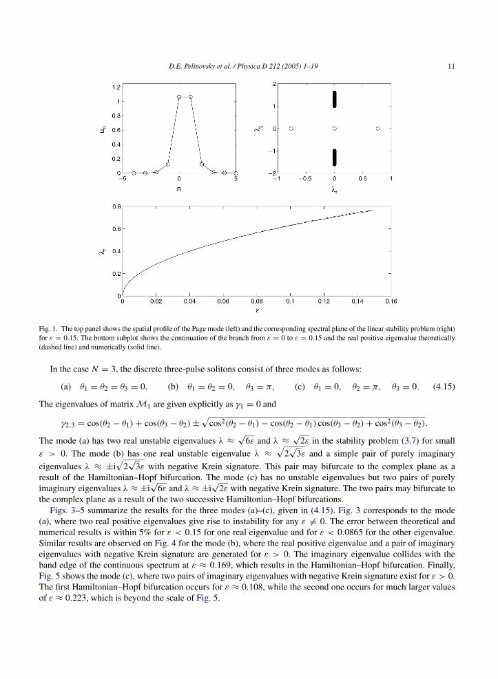
These results are illustrated in Figs. 1 and 2, in agreement with numerical computations of the full problems(2.8) and (3.2). Fig. 1 shows the Page mode, while Fig. 2 corresponds to the twisted mode. The top subplots of eachfigure show the mode profiles (left) and the spectral plane λ = λr + iλi of the linear eigenvalue problem (right) forε = 0.15. The bottom subplots indicate the corresponding real (for the Page mode) and imaginary (for the twistedmode) eigenvalues from the theory (dashed line) versus the full numerical result (solid line). We find the agreementbetween the theory and the numerical computation to be excellent in the case of the Page mode (Fig. 1). For thetwisted mode (Fig. 2), the agreement is within the 5% error for ε < 0.0258. For larger values of ε, the differencebetween the theory and numerics grows. The imaginary eigenvalues collide at ε ≈ 0.146 with the band edge of thecontinuous spectrum such that the real part λr becomes non-zero for ε > 0.146.
D.E. Pelinovsky et al. / Physica D 212 (2005) 1–19 11
Fig. 1. The top panel shows the spatial profile of the Page mode (left) and the corresponding spectral plane of the linear stability problem (right)for ε = 0.15. The bottom subplot shows the continuation of the branch from ε = 0 to ε = 0.15 and the real positive eigenvalue theoretically(dashed line) and numerically (solid line).
In the case N = 3, the discrete three-pulse solitons consist of three modes as follows:
(a) θ1 = θ2 = θ3 = 0, (b) θ1 = θ2 = 0, θ3 = π, (c) θ1 = 0, θ2 = π, θ3 = 0. (4.15)
The eigenvalues of matrixM1 are given explicitly as γ1 = 0 and
γ2,3 = cos(θ2 − θ1) + cos(θ3 − θ2) ±
√cos2(θ2 − θ1) − cos(θ2 − θ1) cos(θ3 − θ2) + cos2(θ3 − θ2).
The mode (a) has two real unstable eigenvalues λ ≈√
6ε and λ ≈√
2ε in the stability problem (3.7) for smallε > 0. The mode (b) has one real unstable eigenvalue λ ≈
√2√
3ε and a simple pair of purely imaginaryeigenvalues λ ≈ ±i
√2√
3ε with negative Krein signature. This pair may bifurcate to the complex plane as aresult of the Hamiltonian–Hopf bifurcation. The mode (c) has no unstable eigenvalues but two pairs of purelyimaginary eigenvalues λ ≈ ±i
√6ε and λ ≈ ±i
√2ε with negative Krein signature. The two pairs may bifurcate to
the complex plane as a result of the two successive Hamiltonian–Hopf bifurcations.Figs. 3–5 summarize the results for the three modes (a)–(c), given in (4.15). Fig. 3 corresponds to the mode
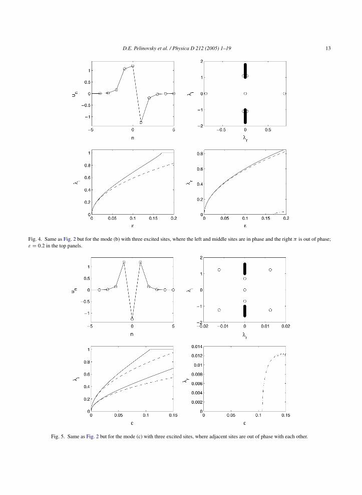
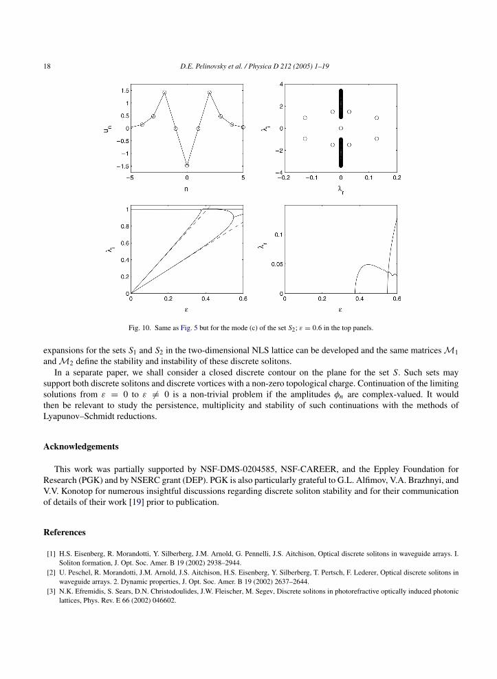
(a), where two real positive eigenvalues give rise to instability for any ε 6= 0. The error between theoretical andnumerical results is within 5% for ε < 0.15 for one real eigenvalue and for ε < 0.0865 for the other eigenvalue.Similar results are observed on Fig. 4 for the mode (b), where the real positive eigenvalue and a pair of imaginaryeigenvalues with negative Krein signature are generated for ε > 0. The imaginary eigenvalue collides with theband edge of the continuous spectrum at ε ≈ 0.169, which results in the Hamiltonian–Hopf bifurcation. Finally,Fig. 5 shows the mode (c), where two pairs of imaginary eigenvalues with negative Krein signature exist for ε > 0.The first Hamiltonian–Hopf bifurcation occurs for ε ≈ 0.108, while the second one occurs for much larger valuesof ε ≈ 0.223, which is beyond the scale of Fig. 5.

12 D.E. Pelinovsky et al. / Physica D 212 (2005) 1–19
Fig. 2. The top panel shows the twisted mode and the spectral plane for ε = 0.16. The bottom subplot shows the imaginary and real parts ofthe eigenvalue with negative Krein signature, which bifurcates to the complex plane at ε ≈ 0.146.
Fig. 3. Same as Fig. 1 but for the mode (a) with three excited sites in phase; ε = 0.15 in the top panels.
D.E. Pelinovsky et al. / Physica D 212 (2005) 1–19 13
Fig. 4. Same as Fig. 2 but for the mode (b) with three excited sites, where the left and middle sites are in phase and the right π is out of phase;ε = 0.2 in the top panels.
Fig. 5. Same as Fig. 2 but for the mode (c) with three excited sites, where adjacent sites are out of phase with each other.
14 D.E. Pelinovsky et al. / Physica D 212 (2005) 1–19
5. Bifurcations of the discrete solitons in the set S2
Here we study the set S2 with the revised perturbation series expansions. The solution is defined by the powerseries (2.9), where the zero-order term φ
(0)n is given by (2.5) with θn = 0, π for all n ∈ S and the first-order term
φ(1)n is given by
φ(1)n = eiθn+1 + eiθn−1 , n = 2m, 1 ≤ m ≤ N − 1,
φ(1)0 = eiθ1 , φ
(1)2N = eiθ2N−1 ,
(5.1)
while all other elements of φ(1)n are zero. The second-order term φ
(2)n solves the inhomogeneous problem
(1 − 3φ(0)2n )φ(2)
n = φ(1)n+1 + φ
(1)n−1 + 3φ(1)2
n φ(0)n , (5.2)
with the unique solution
φ(2)n = −
12(cos(θn+2 − θn) + cos(θn−2 − θn) + 2)eiθn , n = 2m − 1, 2 m ≤ N − 1,
φ(2)1 = −
12(cos(θ3 − θ1) + 2)eiθ1 , φ
(2)2N−1 = −
12(cos(θ2N−1 − θ2N−3) + 2)eiθ2N−1 ,
φ(2)−1 = eiθ1 , φ
(2)2N+1 = eiθ2N−1 ,
(5.3)
while all other elements of φ(2)n are zero. The symmetric matrix H is defined by the power series (3.8), where the
zero-order term H(0) is given by (3.9) and the first-order term H(1) is given by (4.3), where φ(0)n φ
(1)n = 0, n ∈ Z.
The second-order termH(2) has the structure
H(2)n,n = −2φ(0)
n φ(2)n
(3 00 1
), n = 2m − 1, 1 ≤ m ≤ N (5.4)
and
H(2)n,n = −φ(1)2
n
(3 00 1
), n = 2m, 0 ≤ m ≤ N , (5.5)
while all other blocks ofH(2)n,m are zero. Similarly to in the previous section, the semi-simple zero eigenvalue of the
problemHϕ = γϕ is split as ε > 0 according to the modified perturbation series expansion
ϕ = ϕ(0)+ εϕ(1)
+ εϕ(2)+ O(ε3), γ = ε2γ2 + O(ε3), (5.6)
where the zero-order term ϕ(0) is given by (4.5) and the first-order term ϕ(1) has the form
ϕ(1)=
∑n∈S
cn(S+fn + S−fn), (5.7)
where S± are shift operators of the non-zero 2-block of fn up and down. The second-order term ϕ(2) is found fromthe inhomogeneous system
H(0)ϕ(2)= γ2ϕ
(0)−H(1)ϕ(1)
−H(2)ϕ(0). (5.8)
Projecting the system (5.8) onto the kernel ofH(0), we find the reduced eigenvalue problem
M2c = γ2c, (5.9)
where c = (c1, c3, . . . , c2N−1)T andM2 is the tri-diagonal N -by-N matrix, given by
(M2)m,n = (f2m−1,H(2)f2n−1) + (f2m−1,H(1)(S+ + S−)f2n−1), (5.10)
D.E. Pelinovsky et al. / Physica D 212 (2005) 1–19 15
for 1 ≤ n, m ≤ N , or explicitly, based on the first-order and second-order solutions (5.1) and (5.3):
(M2)n,n = cos(θ2n+1 − θ2n−1) + cos(θ2n−3 − θ2n−1), 1 < n < N ,
(M2)n,n+1 = (M2)n+1,n = − cos(θ2n+1 − θ2n−1), 1 ≤ n < N ,
(M2)1,1 = cos(θ3 − θ1), (M2)N ,N = cos(θ2N−1 − θ2N−3).
(5.11)
Similarly, the multiple zero eigenvalue of the problem JHψ = λψ is split as ε > 0 according to the modifiedperturbation series expansion
ψ = ψ (0)+ εψ (1)
+ ε2ψ (2)+ O(ε3), λ = ελ1 + ε2λ2 + O(ε3), (5.12)
where the zero-order term ψ (0)= ϕ(0) is given by (4.5) and the first-order term ψ (1) has the form
ψ (1)=
∑n∈S
cn(S+fn + S−fn) +λ1
2
∑n∈S
cngn . (5.13)
The second-order term ψ (2) is found from the inhomogeneous system
JH(0)ψ (2)= λ1ψ
(1)+ λ2ψ
(0)− JH(1)ψ (1)
− JH(2)ψ (0). (5.14)
Projecting the system (5.14) onto the kernel of JH(0), we find the reduced eigenvalue problem
2M2c = λ21c, (5.15)
in accordance with Lemma 3.1. Since the matrix M2 has exactly the structure of the matrix M1, described inLemma 4.1, we conclude that the stability and instability of the discrete solitons in the set S2 are defined interms of the number n0 of π -differences in θ2n+1 − θ2n−1, 1 ≤ n ≤ N − 1, in accordance with Lemma 3.3 andCorollary 3.5. Thus, Theorem 3.6 for the set S2 is verified with explicit perturbation series results.
We summarize that the bifurcations and stability of the discrete solitons in the set S2 are exactly equivalent tothose in the set S1, but the splitting of all zero eigenvalues occurs in the order of ε2, rather than in the order of ε.These results for the set S2 with N = 2 and N = 3 are shown on Figs. 6–10, in full analogy with those for the setS1. The corresponding asymptotic approximations of eigenvalues can be “translated” from those of the previoussection by substituting
√ε → ε. Fig. 6 shows the Page mode where the agreement with the theory is excellent
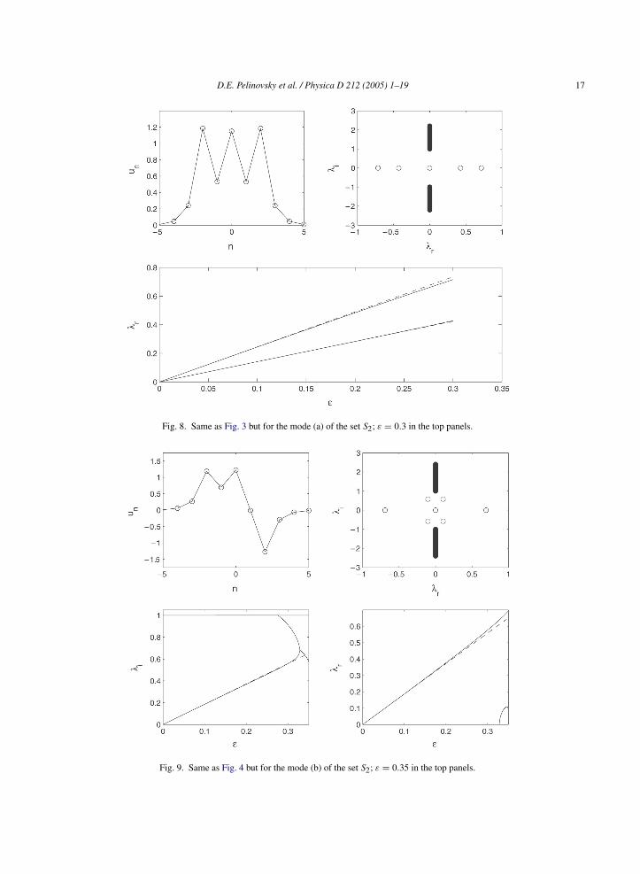
for ε < 0.2. Fig. 7 shows the twisted mode with very good agreement for ε < 0.415 and the Hamiltonian–Hopfbifurcation at ε ≈ 0.431. The only difference from the twisted mode of Fig. 2 is that the imaginary eigenvalue ofnegative Krein signature collides with the imaginary eigenvalue of positive Krein signature, rather than with theband edge of the continuous spectrum. Figs. 8–10 show the modes (a), (b), and (c), respectively, of the three excitedsites. Again, the Hamiltonian–Hopf bifurcations occur when the imaginary eigenvalues of negative Krein signaturecollide with the imaginary eigenvalues of positive Krein signature. For the mode (b), the bifurcation occurs atε ≈ 0.328 (see Fig. 9). For the mode (c), two bifurcations occur at ε ≈ 0.375 and ε ≈ 0.548 (see Fig. 10).
6. Summary
We have studied the stability of discrete solitons in the one-dimensional NLS lattice (1.1) with d = 1. Wehave rigorously proved the numerical conjecture that the discrete solitons with anti-phase excited nodes are stablenear the anti-continuum limit, while all other discrete solitons are linearly unstable with real positive eigenvaluesin the stability problem. Additionally, we gave a precise count of the real eigenvalues and pairs of imaginaryeigenvalues with negative Krein signature. These results are not affected if the excited nodes are separated by anarbitrary sequence of empty nodes. We studied two particular sets of discrete solitons with explicit perturbationseries expansions and numerical approximations and found very good agreement between the asymptotic andnumerical computations.

16 D.E. Pelinovsky et al. / Physica D 212 (2005) 1–19
Fig. 6. Same as Fig. 1 but for the Page mode of the set S2; ε = 0.2 in the top panels.
Fig. 7. Same as Fig. 2 but for the twisted mode of the set S2; ε = 0.6 in the top panels.
The stability and instability results remain invariant if the discrete solitons are excited in the two-dimensionalNLS lattice (1.1) with d = 2 such that the set S is an open discrete contour on the plane. Similar perturbation series
D.E. Pelinovsky et al. / Physica D 212 (2005) 1–19 17
Fig. 8. Same as Fig. 3 but for the mode (a) of the set S2; ε = 0.3 in the top panels.
Fig. 9. Same as Fig. 4 but for the mode (b) of the set S2; ε = 0.35 in the top panels.
18 D.E. Pelinovsky et al. / Physica D 212 (2005) 1–19
Fig. 10. Same as Fig. 5 but for the mode (c) of the set S2; ε = 0.6 in the top panels.
expansions for the sets S1 and S2 in the two-dimensional NLS lattice can be developed and the same matricesM1andM2 define the stability and instability of these discrete solitons.
In a separate paper, we shall consider a closed discrete contour on the plane for the set S. Such sets maysupport both discrete solitons and discrete vortices with a non-zero topological charge. Continuation of the limitingsolutions from ε = 0 to ε 6= 0 is a non-trivial problem if the amplitudes φn are complex-valued. It wouldthen be relevant to study the persistence, multiplicity and stability of such continuations with the methods ofLyapunov–Schmidt reductions.
Acknowledgements
This work was partially supported by NSF-DMS-0204585, NSF-CAREER, and the Eppley Foundation forResearch (PGK) and by NSERC grant (DEP). PGK is also particularly grateful to G.L. Alfimov, V.A. Brazhnyi, andV.V. Konotop for numerous insightful discussions regarding discrete soliton stability and for their communicationof details of their work [19] prior to publication.
References
[1] H.S. Eisenberg, R. Morandotti, Y. Silberberg, J.M. Arnold, G. Pennelli, J.S. Aitchison, Optical discrete solitons in waveguide arrays. I.Soliton formation, J. Opt. Soc. Amer. B 19 (2002) 2938–2944.
[2] U. Peschel, R. Morandotti, J.M. Arnold, J.S. Aitchison, H.S. Eisenberg, Y. Silberberg, T. Pertsch, F. Lederer, Optical discrete solitons inwaveguide arrays. 2. Dynamic properties, J. Opt. Soc. Amer. B 19 (2002) 2637–2644.
[3] N.K. Efremidis, S. Sears, D.N. Christodoulides, J.W. Fleischer, M. Segev, Discrete solitons in photorefractive optically induced photoniclattices, Phys. Rev. E 66 (2002) 046602.
D.E. Pelinovsky et al. / Physica D 212 (2005) 1–19 19
[4] A.A. Sukhorukov, Yu.S. Kivshar, H.S. Eisenberg, Y. Silberberg, Spatial optical solitons in waveguide arrays, IEEE J. Quantum Electron.39 (2003) 31–50.
[5] F.S. Cataliotti, S. Burger, C. Fort, P. Maddaloni, F. Minardi, A. Trombettoni, A. Smerzi, M. Inguscio, Josephson junction arrays withBose–Einstein condensates, Science 293 (2001) 843–846.
[6] F.S. Cataliotti, L. Fallani, F. Ferlaino, C. Fort, P. Maddaloni, M. Inguscio, Superfluid current disruption in a chain of weakly coupledBose–Einstein condensates, New J. Phys. 5 (2003) 71.
[7] F.Kh. Abdullaev, B.B. Baizakov, S.A. Darmanyan, V.V. Konotop, M. Salerno, Nonlinear excitations in arrays of Bose–Einsteincondensates, Phys. Rev. A 64 (2001) 043606.
[8] G.L. Alfimov, P.G. Kevrekidis, V.V. Konotop, M. Salerno, Wannier functions analysis of the nonlinear Schrodinger equation with aperiodic potential, Phys. Rev. E 66 (2002) 046608.
[9] M.V. Fistul, Resonant breather states in Josephson coupled systems, Chaos 13 (2003) 725–732.[10] J.J. Mazo, T.P. Orlando, Discrete breathers in Josephson arrays, Chaos 13 (2003) 733–743.[11] T. Dauxois, M. Peyrard, A.R. Bishop, Entropy-driven DNA denaturation, Phys. Rev. E 47 (1993) R44–R47.[12] M. Peyrard, T. Dauxois, H. Hoyet, C.R. Willis, Biomolecular dynamics of DNA–Statistical-mechanics and dynamical models, Phys. D 68
(1993) 104–115.[13] S. Aubry, Breathers in nonlinear lattices: existence, linear stability and quantization, Phys. D 103 (1997) 201–250.[14] S. Flach, C.R. Willis, Discrete breathers, Phys. Rep. 295 (1998) 181–264.[15] D. Hennig, G. Tsironis, Wave transmission in nonlinear lattices, Phys. Rep. 307 (1999) 333–432.[16] P.G. Kevrekidis, K.O. Rasmussen, A.R. Bishop, The discrete nonlinear Schrodinger equation: A survey of recent results, Int. J. Mod. Phys.
B 15 (2001) 2833–2900.[17] J.Ch. Eilbeck, M. Johansson, in: L. Vazquez, R.S. MacKay, M.P. Zorzano (Eds.), Localization and Energy Transfer in Nonlinear Systems,
World Scientific, Singapore, 2003, p. 44.[18] M. Peyrard, Yu.S. Kivshar, Modulational instabilities in discrete lattices, Phys. Rev. A 46 (1992) 3198–3205.[19] G.L. Alfimov, V.A. Brazhnyi, V.V. Konotop, On classification of intrinsic localized modes for the discrete nonlinear Schrodinger equation,
Phys. D 194 (2004) 127–150.[20] H.R. Dullin, J.D. Meiss, Generalized Henon maps: the cubic diffeomorphisms of the plane, Phys. D 143 (2000) 262–289.[21] J.M. Bergamin, T. Bountis, C. Jung, A method for locating symmetric homoclinic orbits using symbolic dynamics, J. Phys. A: Math. Gen.
33 (2000) 8059–8070.[22] J.M. Bergamin, T. Bountis, M.N. Vrahatis, Homoclinic orbits of invertible maps, Nonlinearity 15 (2002) 1603–1619.[23] S. Aubry, G. Abramovici, Chaotic trajectories in the standard map—the concept of antiintegrability, Phys. D 43 (1990) 199–219.[24] R.S. MacKay, S. Aubry, Proof of existence of breathers for time-reversible or Hamiltonian networks of weakly coupled oscillators,
Nonlinearity 7 (1994) 1623–1643.[25] L. Nirenberg, Topics in Nonlinear Functional Analysis, Courant Institute, NY, 1974.[26] M. Weinstein, Excitation thresholds for nonlinear localized modes on lattices, Nonlinearity 12 (1999) 673–691.[27] T. Kapitula, P.G. Kevrekidis, Stability of waves in discrete systems, Nonlinearity 14 (2001) 533–566.[28] M. Johansson, S. Aubry, Existence and stability of quasiperiodic breathers in the discrete nonlinear Schrodinger equation, Nonlinearity
10 (1997) 1151–1178.[29] P.G. Kevrekidis, A.R. Bishop, K.O. Rasmussen, Twisted localized modes, Phys. Rev. E 63 (2001) 036603.[30] T. Kapitula, P.G. Kevrekidis, B.A. Malomed, Stability of multiple pulses in discrete systems, Phys. Rev. E 63 (2001) 036604.[31] P.G. Kevrekidis, M.I. Weinstein, Breathers on a background: periodic and quasiperiodic solutions of extended discrete nonlinear wave
systems, Math. Comput. Simulation 62 (2003) 65–78.[32] A.M. Morgante, M. Johansson, G. Kopidakis, S. Aubry, Standing wave instabilities in a chain of nonlinear coupled oscillators, Phys. D
162 (2002) 53–94.[33] M. Johansson, Hamiltonian Hopf bifurcations in the discrete nonlinear Schrodinger equation, J. Phys. A: Math. Gen. 37 (2004) 2201–2222.[34] B. Sandstede, C.K.R.T. Jones, J.C. Alexander, Existence and stability of N -pulses on optical fibers with phase-sensitive amplifiers, Phys.
D 106 (1997) 167–206.[35] B. Sandstede, Stability of multiple-pulse solutions, Trans. Amer. Math. Soc. 350 (1998) 429–472.[36] T. Kapitula, Stability of waves in perturbed Hamiltonian systems, Phys. D 156 (2001) 186–200.[37] T. Kapitula, P.G. Kevrekidis, Linear stability of perturbed Hamiltonian systems: theory and a case example, J. Phys. A: Math. Gen. 37
(2004) 7509–7526.[38] R. Horn, C. Johnson, Matrix Analysis, Cambridge University Press, 1985.[39] H. Levy, F. Lessman, Finite Difference Equations, Dover, New York, 1992.[40] D. Pelinovsky, Inertia law for spectral stability of solitary waves in coupled nonlinear Schrodinger equations, Proc. Roy. Soc. Lond. A
461 (2005) 783–812. Preprint available at http://dmpeli.math.mcmaster.ca/PaperBank/diagonalization.pdf.[41] T. Kapitula, P.G. Kevrekidis, B. Sandstede, Counting eigenvalues via the Krein signature in infinite-dimensional Hamiltonian systems,
Phys. D 195 (2004) 263–282.