Stability Analysis of Parallel DC-DC Converters - …mazumder/14.pdf · Stability Analysis of...

Stability Analysis of ParallelDC-DC Converters

SUDIP K. MAZUMDER, Senior Member, IEEEUniversity of Illinois at Chicago

We develop analytic methodologies for stability analyses (using

nonlinear and linear methodologies) of parallel dc-dc converters

(under unsaturated and saturated operating conditions) using

their switching model, discrete model (based on nonlinear map),

and averaged model. We describe the approach for investigating

the behavior of the stable and unstable equilibrium solutions

of a parallel dc-dc converter under parametric variations and

illustrate the methodology using a load-sharing dc-dc buck

converter. For unsaturated operating condition, using bifurcation

analysis and Floquet theory, we predict the stability boundary of

the nominal solution, determine its postinstability dynamics, and

investigate the dependence of the converter dynamics on its initial

conditions. Subsequently, we demonstrate the differences in the

predictions of the instabilities and instability boundaries using

(conventional) linearized averaged (small-signal) and discrete and

switching models.

Manuscript received September 27, 2003; revised May 31 andSeptember 3, 2005; released for publication September 3, 2005.

IEEE Log No. T-AES/42/1/870591.

Refereeing of this contribution was handled by W. M. Polivka.

This work was supported in part by the National ScienceFoundation CAREER Award received by Professor Mazumder in2003 under Award 0239131.

Author’s address: Dept. of Electrical and Computer Engineering,MC 154, 1020 Science and Engineering Offices, University ofIllinois at Chicago, 851 S. Morgan St., Chicago, IL 60607-7053,E-mail: ([email protected]).

0018-9251/06/$17.00 c° 2006 IEEE

I. INTRODUCTION

Parallel dc-dc converters are widely used intelecommunication power supplies [32]. They operateunder closed-loop feedback control to regulatethe output voltage and enable load sharing. Theseclosed-loop converters are inherently nonlinearsystems. The major sources of nonlinearities are theswitching nonlinearity and converter interaction. Sofar, however, analyses in this area of power electronicsare based primarily on linearized (small-signal)averaged models. When a nonlinear converter hassolutions other than the nominal one, small-signalanalyses cannot predict the basin of attraction of thenominal solution and the dynamics of the system afterthe nominal solution loses stability. The dependenceof the converter dynamics on the initial conditionsis also ignored in small-signal analyses. In addition,averaged models cannot predict the dynamics of aswitching converter in a saturated region.To analyze the stability of these switching systems,

one has to deal first with their discontinuity [24, 31].The concept of stability of the equilibrium solutionsof a continuous, smooth system is well defined [1, 2].However, for discontinuous systems, the definition ofsolution is itself not straightforward [3—5]. To analyzethe stability of an n-dimensional discontinuous systemwith m switching planes, one has to first define aregion of operation, which in general lies at theintersection of these m hyperplanes. The globalstability of this region is defined as follows [4]. Onehas to show first that all of the trajectories approachthis region (reaching condition) and that, once onthis hypersurface, they cannot leave it (existencecondition). If these two conditions are satisfied, thenthe discontinuous system has a solution surface ora sliding mode. The dynamics of the system on thishypersurface is described by a set of equations, whichare smooth and continuous. Finally, one has to showthat all of the solutions on this surface tend to a singleequilibrium point as time t!1.Analysis of a variable-structure system using an

averaged model assumes two things. First, a solutionsurface exists. In other words, the reaching andexistence conditions are satisfied. Second, the controlhas no delay or the switching frequency is infinite. Inreality, the switching frequency is finite and for manyconverters global existence of a solution surface forany controller is not possible.If the frequency is finite, then we do not have a

solution surface but a boundary layer around it [5].Thus stability in the sense of Filippov [4] can beapplied only if the width of the boundary layer iszero. Under this condition, the dynamics of the systemon the solution surface are described accurately bythe averaged model. However, when the width of theboundary layer is not zero, we convert the periodicsystem to a map. Thus, within the boundary layer, we

50 IEEE TRANSACTIONS ON AEROSPACE AND ELECTRONIC SYSTEMS VOL. 42, NO. 1 JANUARY 2006

redefine the stability problem from one of analyzingthe stability of a periodic orbit to that of analyzing thestability of a fixed point.We use these basic concepts to investigate the local

and global stabilities of nonlinear, nonautonomousparallel dc-dc converters in the unsaturated andsaturated regions.1 Unlike [32] and [33], the analysespresented here are generalized and the conceptfeasibility is illustrated for a simple two-converterproblem using commonly-used averaged-currentsharing control instead of master-slave control in [33].The present paper also outlines stability approachesusing switching, discrete, and averaged model forparallel dc-dc converters. Further, unlike [32] and[33], the analyses have been presented here forunsaturated as well saturated regions. Within theunsaturated region, we develop techniques to predictthe fast-scale and slow-scale stability boundariesand to determine the type of instability of thenominal orbit. Using these ideas, instabilities of twoclosed-loop buck converters operating in phase andwith interleaving are investigated, which is also a keydifference of the present work compared with [33].For these two cases, we compare the results obtainedusing a nonlinear map with those obtained using theaveraged model and demonstrate the shortcomings ofthe latter. Unlike [33], we also demonstrate the impactof parametric variations of the parallel converter onits fast-scale and slow-scale instabilities. Finally,we investigate the impact of a strong feedforwarddisturbance on the stability of the two buck converterswhen they have the same parameters and when theyhave parametric variation. Using concepts developedin this paper, we predict the dynamics of the converterin the saturated and unsaturated regions understeady-state and transient conditions. The presentedstability problem is a real phenomenon, which couldoccur in any practical multi-module converter systemand the results presented can be used to predict andprevent such a problem.

II. MODELING

A. Power Stage

We assume that the nonlinearities due to thepower devices and parasitics are negligible and thatthe converter, operating in continuous conductionmode (CCM),2 is clocked at a rate equal to the

1A comprehensive stability analysis using nonlinear map for asingle dc-dc converter (i.e., N = 1 in Section II) is provided in [9].2If the parallel dc-dc operates in discontinuous conduction mode(DCM), the map-based analysis approach described here remainsexactly the same; only the map and the auxiliary switchingconditions change. Likewise, the switching and the averaged modelsof the parallel dc-dc converters will change, but the basic stabilityanalysis approach remains unchanged.

Fig. 1. Generic configuration of N parallel dc-dc convertersoperating with single voltage source and load.

switching frequency. Moreover, the controller isdesigned in such a way that, once a change of stateis latched, it can be reset only by the next clock.This effectively eliminates the possibility of multiplepulses within a switching cycle. In Fig. 1 we show aschematic of a generic basic parallel dc-dc converterwith one switch per converter. The total number ofconverters connected in parallel is N. Each individualmodule within these multi-topological systems isin the on-state when the switch is closed and in theoff-state when it is open. We represent these switchingfunctions by a switching vector S(t). We assume thatthe phase shift between the carrier waveforms of twosuccessive converters is equal to ± = T=N, which isconstant (where T is the switching cycle time). Wenote that, when ± = 0, the converters are switchingin phase. If we represent the states of the open-loopconverter (i.e., the inductor currents iLi (t) and thecapacitor voltages vCi (t) by the vector X

o(t), then theequations governing a parallel-boost or a parallel-buckconverter can be expressed as

_Xo(t) = Fo1 (Xo(t),u(t),S(t))

vdc(t) = Fo2 (X

o(t),u(t),S(t))(1)

where u(t) is the forcing input. Equation (1) representsa discontinuous and nonautonomous system. The

MAZUMDER: STABILITY ANALYSIS OF PARALLEL DC-DC CONVERTERS 51

discontinuity is due to the switching vector S(t). Forconvenience, we drop the notation of time from nowon and rewrite (1) as

_Xo = Fo(Xo,u)+Go(Xo,u)S+Wo1 (X

o,S)

vdc =Ho(Xo)+Wo

2 (Xo,S)

(2)

where Fo, Go, and Ho are continuous functions. Forsome systems (e.g., the parallel-buck converter), Wo

1and Wo

2 are continuous because terms containing theequivalent series resistance (ESR) are not coupledwith the switching function. Hence, Wo

1 and Wo2 can

be lumped with the other terms in (2). However, forother systems like the parallel-boost converter, theyare discontinuous. If we neglect the ESR, then (2)simplifies to the following form:

_Xo = Fo(Xo,u) +Go(Xo,u)S

vdc =Ho(Xo):

(3)

Equations (2) and (3) represent generic switchingmodels of parallel-buck and parallel-boost converterswhen the effect of the ESR is incorporated and whenit is not.An alternate way to model the variable-structure

system represented by (2) is to use a map [6—9].Because there are N converters (as illustrated in Fig. 2for N = 2), which are operating in parallel with aphase shift of ±, there are N switchings that occur ineach switching cycle (of duration T) of the nominalsteady-state system. The state-space equations for theith subswitching cycle of duration ti are written as

_Xo = Aoi Xo +Boi u

vdc = Coi X

o(4)

whereNXi=1

ti = T (5)

and Aoi , Boi , and C

oi are matrices that describe the

open-loop system in the time interval ti [9]. Ineach switching subcycle, these matrices can beobtained from (2) by substituting an appropriatevector consisting of binary numbers for the switchingvector S.Next, we derive an exact solution of the open-loop

system by stacking the consecutive solutions of (4)over a switching period. The resulting discrete-timeequation can be written in state-space form as

Xok+1 = fo1 (X

ok , t1, t2, : : : , t2N ,uk)

=©o(t1, t2, : : : , t2N)Xok +¡

o(t1, t2, : : : , t2N)uk

vdck+1 = fo2 (X

ok , t1, t2, : : : , t2N ,uk) = C

o2NX

ok+1

(6)

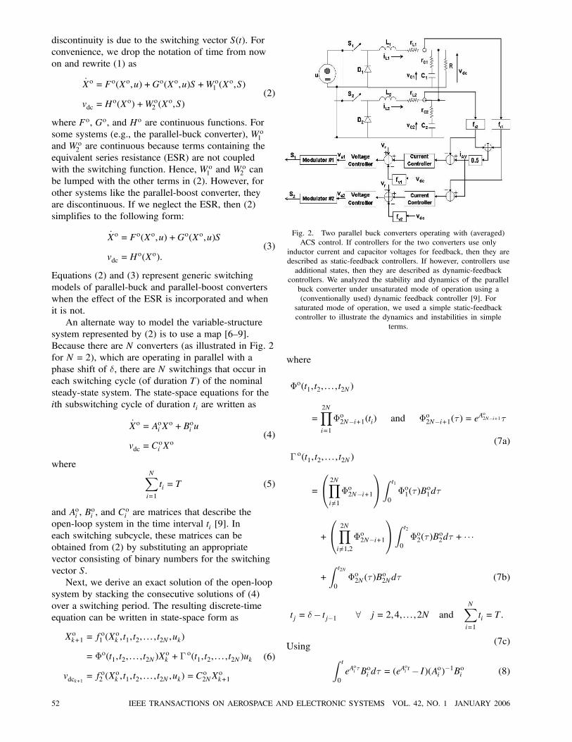
Fig. 2. Two parallel buck converters operating with (averaged)ACS control. If controllers for the two converters use only

inductor current and capacitor voltages for feedback, then they aredescribed as static-feedback controllers. If however, controllers useadditional states, then they are described as dynamic-feedback

controllers. We analyzed the stability and dynamics of the parallelbuck converter under unsaturated mode of operation using a(conventionally used) dynamic feedback controller [9]. For

saturated mode of operation, we used a simple static-feedbackcontroller to illustrate the dynamics and instabilities in simple

terms.

where

©o(t1, t2, : : : , t2N)

=2NYi=1

©o2N¡i+1(ti) and ©o2N¡i+1(¿ ) = eAo2N¡i+1¿

(7a)

¡ o(t1, t2, : : : , t2N)

=

0@ 2NYi 6=1©o2N¡i+1

1AZ t1

0©o1(¿)B

o1d¿

+

0@ 2NYi 6=1,2

©o2N¡i+1

1AZ t2

0©o2(¿)B

o2d¿ + ¢ ¢ ¢

+Z t2N

0©o2N(¿)B

o2Nd¿ (7b)

tj = ±¡ tj¡1 8 j = 2,4, : : : ,2N andNXi=1

ti = T:

(7c)Using Z t

0eA

oi¿Boi d¿ = (e

Aoit¡ I)(Aoi )¡1Boi (8)


and (7), we simplify the expression for Xok+1 in(6) to

Xok+1 = fo1 (X

ok , t1, t2, : : : , t2N ,uk)

=2NYi=1

eAoit2N¡i+1Xok

+

0BBBBBBB@

Ã2NYi 6=1eA

o2N¡i+1 ti

!(eA

o1t1 ¡ I)(Ao1)¡1Bo1

+

Ã2NYi 6=1,2

eAo2N¡i+1 ti

!(eA

o2t2 ¡ I)(Ao2)¡1Bo2

+ ¢ ¢ ¢+(eAo2N t2N ¡ I)(Ao2N)¡1Bo2N

1CCCCCCCAuk:

(9)

Equations (6) and (9) describing vdck+1 andXok+1 represent a map for dc-dc parallel-buck andparallel-boost converter. If we compare the mapwith the switching model described in (2), we seethat the map does not have the discontinuities dueto the switching vector S. This helps in studying thedynamics because the concept of solution for smoothsystems is well defined. Besides, simulations basedon this map are much faster since they correlate thestates in one switching cycle (of duration T) withthose in the next switching cycle. Because the mapis not dependent on time any more, it describes areduced-order system. Hence, it cannot predict thedynamics of a parallel converter beyond half theswitching frequency. However, it can predict thesubharmonics accurately.Another approach to modeling parallel converters

is based on state-space averaging [10, 11]. In thiscase, we convert the discontinuous-differential systemof equations described by (2) to a continuous systemby replacing the vector representing the switchingfunctions with a smooth and continuous duty-ratiovector. In Appendix A, we illustrate the derivationof an averaged model with two examples based on aparallel-buck converter operating with two differentswitching schemes. The general expression for theaveraged model is

_Xo

= Fo(Xo, u) +Go(Xo, u)+Wo1av (X

o,D)

vdc =Ho(Xo)+Wo

2av (Xo,D)

(10)

where Wo1avand Wo

2avare continuous functions and Xo

represents the averaged value of the open-loop states.The symbol D is a vector, which denotes the dutyratios of a parallel converter. For some converters(e.g., parallel buck), Wo

1av and Wo2av are independent

of D. Hence, they can be lumped with Fo and Ho.However, for others, like parallel boost converters,they depend on D. Equation (10), describes a systemof ordinary differential equations, which can be usedfor investigating only slow-scale dynamics.

B. Controller

There are more than one scheme for parallelingdc-dc converters [27—30], including the master-slavemethod [12] and the active-current sharing method[13, 14]. The objectives of all of these schemes, ingeneral, are to regulate the output voltage and sharethe load power equally among the converters. Thestability techniques we develop here are generic.However, due to lack of space, we present simulationresults for the performance of parallel convertersoperating with an active-current sharing (ACS)scheme.In Fig. 2, we show a schematic for an ACS

control. The symbol iav represents the average ofall load currents. To share the load equally amongthe converters, the error between iav and the loadcurrent supplied by each converter is added to thereference voltage vr. The updated voltage referenceis then compared with the output voltage for eachconverter. The output of the voltage loop is comparedwith the inductor current, which is the controllererror signal. The controller can be simplified on theneed and application. If we consider a static-feedbackcontroller, then the expression of the error signal foreach converter can be expressed as

vei = Psi X

o + vr (11)

where Psi is a matrix corresponding to thestatic-feedback controller. If, however, we considera dynamic-feedback controller, then we obtain

vei = Pdi X

c: (12)

In (12), Xc represents the additional states of thedynamics-feedback controller and is given by

_Xc = AcXaug +Bcu+Brcvr (13)

where Xaug = (Xo Xc)T, Ac is a matrix, and Bc andBrc are column vectors. Equations (11)—(13) give theexpressions for a multiloop static/dynamic feedbackcontroller. If the multiloop system does not use aninner inductor-current loop then the matrices in(11)—(13) have to be modified.

III. CLOSED-LOOP PARALLEL DC-DC CONVERTER

For a static-feedback controller, the order of theclosed-loop and open-loop systems remains the same.The closed-loop switching model for the parallelconverter is given by

_X = F(X,u,vr)+G(X,u)S+W1(X,S)

vdc =H(X)+W2(X,S)(14)

where F, G, and H are continuous functions.The functions W1 and W2 are continuous for the


parallel-buck converter and discontinuous for theparallel-boost converter. For a static-feedbackcontroller, X = Xo. But for a dynamic-feedbackcontroller X = Xaug. The individual components ofthe switching vector S are given by

si =−i(vei ¡ vrampi(t,±)) (15)

where individual ramp signals are described asfollows:

vrampi (t,±) = vmi ¤mod(t+(i¡ 1)±,T)¤f

8 i= 1, : : : ,N and f = 1=T:(16)

Equation (16) describes the equations for carrierwaveforms with amplitudes vmi . Each of these rampwaveforms has a period of T. Between the twocarrier waveforms, there is a phase shift ±. It followsfrom (15) that the si are functions of the states ofthe closed-loop converter. Hence, the closed-loopswitching model in (14) represents a nonlinearnonautonomous discontinuous system.Next, we derive a nonlinear map based on (14).

The state-space equation for the ith subswitching cycle(of duration ti) is written as

_X = AiX +Biu+Bri vr

vdc = CiX(17)

whereNXi=1

ti = T (18)

and Ai, Bi, Bri , and Ci and are matrices that describe

the closed-loop system in each subcycle. In eachswitching subcycle, these matrices can be obtainedfrom (14) by substituting an appropriate vectorconsisting of binary numbers for the switching vectorS. Next, we derive an exact solution of the closed-loopsystem by stacking the consecutive solutions of (17)over a switching period. The resulting discrete-timedifference equation can be written in state-space formas

Xk+1 = f1(Xk, t1, t2, : : : , t2N ,uk)

=2NYi=1

eA2N¡i+1 tiXk

+

0BBBBBBBB@

Ã2NYi 6=1eA2N¡i+1 ti

!(eA1 t1 ¡ I)(A1)¡1B1

+

Ã2NYi 6=1,2

eA2N¡i+1 ti

!(eA2 t2 ¡ I)(A2)¡1B2

+ ¢ ¢ ¢+(eA2N t2N ¡ I)(A2N)¡1B2N

1CCCCCCCCAuk

+

0BBBBBBB@

Ã2NYi 6=1eA2N¡i+1 ti

!(eA1t1 ¡ I)(A1)¡1Br1

+

Ã2NYi 6=1,2

eA2N¡i+1 ti

!(eA2t2 ¡ I)(A2)¡1Br2

+ ¢ ¢ ¢+(eA2N t2N ¡ I)(A2N)¡1Br2N

1CCCCCCCAvr

(19a)

vdck+1 = f2(Xk, t1, t2, : : : , t2N ,uk,vr) = C2NXk+1 (19b)

¾(Xk, t1, t2, : : : , t2N ,uk,vr) = 0 (19c)

and

tj = ±¡ tj¡1 8 j = 2,4, : : : ,2N: (19d)

In (19c), ¾ is a vector of dimension N £ 1 andrepresents the auxiliary switching conditions for all ofthe converters. For instance, the switching conditionfor the converter that switches first is given by

¾(Xk, t1,uk,vr)

= '¡ (eA1 t1ªk +(eA1t1 ¡ I)A¡11 (B1uk +Br1vr))¡ vramp1 t1 = 0(20)

where the vector ' represents the controller. Using(19d), we reduce the dimension of ¾ to N.Finally, we obtain an averaged model for the

closed-loop system. Using the same methodology,which was used to develop the averaged model forthe open-loop converter, we show that the closed-loopaveraged model for the parallel converter is given bythe following expressions:

_X = F(X, u,vr) +G(X, u)D+W1av (X,D)

vdc =H(X) +W2av (X,D)

di =1

vrampivei = PiX

(21)

where W1av and W2av are continuous functions, Pirepresents a matrix, and D is a vector representing theduty ratios of the converters operating in parallel. Theindividual components of this vector D are given by diin (21). Equation (21) represents a nonlinear averagedmodel. It can be used for studying the slow-scaleinstability. If the ESRs of the output capacitors areneglected, the averaged model cannot distinguishbetween the dynamics of interleaved and synchronizedconverters. Moreover, the averaged model cannot beused to study the impact of saturation.

IV. ANALYSIS

In this section, we show how to analyze the localand global stability of the dynamics of a paralleldc-dc converter operating in the unsaturated andsaturated regions. The parallel converters, shownin Fig. 1, operate with a finite switching frequency.


The dynamics of these discontinuous nonlinearnonautonomous systems evolve on fast and slowscales. The stability analysis of these discontinuoussystems is difficult because the definition of a solutionis not clearly defined.Filippov [4] and Aubin and Cellina [3] proposed

differential inclusion to find solutions of suchdiscontinuous systems with a multivalued right-handside. The resulting solution of this set-valued mapdescribes a solution of the slow dynamics [3] Theaveraged model in (21) approximately describes theslow dynamics for two reasons. First, the switchingfrequencies of the systems are finite. Hence, they donot have a discontinuous surface but a boundary layeraround the discontinuity. The averaged model in (21)is based on the assumption of an infinite frequencyand hence the width of the boundary layer is zero.Second, because switching of the converters in Figs. 1and 2 is based on a comparison of an error signalwith a ramp rather than a hysteresis, the equivalentcontrol approach proposed by Filippov (which formsthe basis for (21)) is not always directly applicable[5]. However, an analysis using an averaged model isstraightforward because it is continuous and smooth.We deal with the stability based on an averaged modellater in this section.An alternate way to analyze the stability of these

variable-structure systems is to use the nonlinearmap in (19). We describe the evolution of thediscontinuous system as a sequence. Besides, weeliminate the discontinuity due to switching bypredicting the states at the beginning of the nextswitching cycle based on the information availableat the end of the current switching cycle. Using thesemaps, we convert the problem of finding the stabilityof a nominal orbit (period-one orbit) to that of findingthe stability of a fixed point.Another way to investigate the stability of the

nominal solution of (14) is numerical computation.We transform (14) to the following form:

Xk+1 =M1(Xk, t0k, t0k+1,uk,vr): (22)

By choosing a relatively small time step t0k+1¡ t0k,one can obtain a fairly accurate solution. In (22),the scalar t0 represents the actual time and not theinstant of switching. How small the time step has tobe depends on how fast the open-loop and closed-loopstates evolve. The degree of accuracy dependsnot only on the time step but also on the type ofnumerical algorithm [15]. It was found that the useof a combination of implicit and explicit numericaltechniques gives the best results. The rationale behindobtaining the solution of a discontinuous system usingnumerical integration is provided by the Lebesguemeasure theory [16]. There are two primary reasonswhy it is applicable here. First, the total number ofswitchings in one switching cycle is finite becausemultiple pulsing cannot occur. Second, at each of

these switching instants, the right- and left-handlimits of each of the states of the converters are equal.This is because we are considering hard-switchedconverters. Thus, at the points of discontinuity, we donot have any jump in the states. Based on these twopieces of information and on whether the samplingtime for numerical integration is much smaller thanthe dynamics of the system, the Lebesgue theory tellsus that we can consider the points of discontinuities(due to switchings) to have zero measure [4, 16]. Inother words, though the system is undefined at thepoints of switching, we can carry out the integrationand the resulting solution is valid almost everywhere.

A. Stability Analysis using the Switching Model

We use a combination of a shooting technique andNewton-Raphson procedure to calculate the periodicorbits and determine their stability. To accomplishthis, we convert the initial-value problem in (14) to atwo-point boundary-value problem. Let the dimensionof X be n£ 1. We seek an initial condition ° = X(0)such that the minimal solution X(t,°) of (14) satisfiesthe condition

X(T,°) = ° = X(0): (23)

In other words, the trajectory that runs from ° =X(0) to the same location over a time period of Trepresents the desired periodic solution.We start with a guess °0 and seek a ±° such that

X(T,°0 + ±°)¡ (°0 + ±°)¼ 0: (24)

Expanding (24) in a Taylor series and keeping onlythe linear terms in ±°, we obtain

(@X°(T,°0)¡ I)±° = °0¡X(T,°0): (25)

In (25), @X°(T,°0) represents the derivatives of X withrespect to ° evaluated at (T,°0). The dimension of thematrix @X°(T,°0) is n£ n. The individual componentsof this matrix are given by

@X°i (T,°0) = limh!0Xi(T,°0 + h°0i )¡X(T,°0)

h:

(26)

Once @X°(T,°0) is known, we solve the system ofn linear algebraic (25) for ±°. Then, we use ±° toupdate the initial guess °0 and repeat the process until±° is within a tolerance level. Finally, the stabilityof the calculated periodic solution is ascertainedfrom the eigenvalues of the monodromy matrix @X°evaluated at (T,°0). For the periodic solution to beasymptotically stable, every eigenvalue but one mustbe inside the unit circle in the complex plane.

B. Stability Analysis using the Discrete Model

Let us assume that the closed-loop systemdescribed by (19) is operating in steady state. The


fixed points of Xk in (19a) correspond to period-oneorbits of the closed-loop converter. They are obtainedusing the constraint Xk+1 = Xk = Xs. Letting us = uk,t1 = t1s , t2 = t2s , : : : , t2N = t2Ns we find that the fixedpoints of (19a) are given by

Xs =

ÃI¡

2NYi=1

eA2N¡i+1 tis

!¡1

£

0BBBBBBBBBB@

0@ 2NYi 6=1eA2N¡i+1 tis

1A(eA1t1s ¡ I)(A1)¡1B1+

0@ 2NYi 6=1,2

eA2N¡i+1 tis

1A (eA2t2s ¡ I)(A2)¡1B2+ ¢ ¢ ¢+(eA2N t2Ns ¡ I)(A2N)¡1B2N

1CCCCCCCCCCAus

+

ÃI¡

2NYi=1

eA2N¡i+1 tis

!¡1

£

0BBBBBBBBBB@

0@ 2NYi 6=1eA2N¡i+1 tis

1A(eA1t1s ¡ I)(A1)¡1Br1+

0@ 2NYi 6=1,2

eA2N¡i+1 tis

1A (eA2t2s ¡ I)(A2)¡1Br2+ ¢ ¢ ¢+(eA2N t2Ns ¡ I)(A2N)¡1Br2N

1CCCCCCCCCCAvr:

(27)

Substituting (27) into (19c), we obtain

¾(Xs, t1s, t2s, : : : , t2Ns,us,vr) = 0: (28)

We solve (27) and (28) for the N unknowns X andthe tis . One way to solve for the unknowns is tosubstitute for Xs from (27) into (28) and solve forthe tis . Once the tis are calculated, we solve for Xs.This is difficult for higher order systems becausemost of the mathematical packages, like Matlab orMathematica, cannot symbolically compute exponentsof very large matrices. Besides, the computation of(I¡Q2N

i=1 eA2N¡i+1 tis) in (27) using these packages is

inaccurate. Alternately, we use a Newton-Raphsonmethod. We start with an initial guess Xg and tig forthe steady-state values of Xs and tis . This guess isobtained using either simulation or the method ofsteepest decent [17]. Keeping the uk constant, werewrite (19a) and (19c) as

Xg + ±Xg = f1(Xg + ±Xg , t1g + ±t1g , t2g + ±t2g , : : : , t2Ng + ±t2Ng )

(29)

¾(Xg + ±Xg, t1g + ±t1g , t2g + ±t2g , : : : , t2Ng + ±t2Ng ) = 0:

(30)

Expanding (29) and (30) in Taylor series, we obtain

Xg + ±Xg = f1(Xg + ±Xg) +@f1@Xg

±Xg +@f1@tg±tg (31)

¾(Xg + ±Xg) +@¾

@Xg±Xg +

@¾

@tg±tg = 0 (32)

where tg is a vector representing t1g , t2g , : : : , t2Ng . Werewrite (31) and (32) as0BB@

@f1@Xg

@f1@Xg

@f1@Xg

@f1@Xg

1CCAµ±Xg±tg¶= J

µ±Xg

±tg

¶=µXg ¡f1¡¾

¶:

(33)

Equation (33) represents a set of linear algebraicequations, which are solved for ±Xg and ±tg by usingthe LU decomposition method [18]. To this end,we express J as LU, where the matrices L and Urepresent the lower and upper triangular matrices ofJ . Then, we rewrite (33) as

J

µ±Xg

±tg

¶= LU

µ±Xg

±tg

¶=µXg ¡f1¡¾

¶: (34)

Multiplying (34) from the left with L¡1, we have

U

µ±Xg

±tg

¶= Z = L¡1

µXg ¡f1¡¾

¶(35)

which can be solved for the new set of variables Z.Then the (±Xg ±tg) are calculated without inverting thematrix U.We found that, unlike the matrix J¡1, the

matrix L¡1 can always be computed correctly byeither Matlab or Mathematica. If, however, thisis not the case, then one can use more advancedalgorithms, such as the conjugate gradient method[18] and globally convergent homotopy algorithms[19]. However, homotopy algorithms have thedisadvantage of giving both the real-valued as wellas the complex-valued solutions.To ascertain the stability of a given fixed point, we

perturb the nominal values as

X = Xs+ ±X, t= ts+ ±t

u= us+ ±u, vdc = vdcs+±vdc :(36)

Substituting (36) into (19a) and (19c), expanding theresults in Taylor series, and keeping first-order terms,we obtain

±Xk+1 =@f1@X

±X +@f1@u±u

@¾

@X±X +

@¾

@t±t+

@¾

@u±u= 0:

(37)


It follows from the second equation of (37) that

±t=¡µ@¾

@t

¶¡1µ @¾@X±X +

@¾

@u±u

¶: (38)

Substituting (38) into the first equation of (37), yields

±Xk+1 =H1±X +H2±u (39)

where

H1 =@f1@X

¡µ@¾

@t

¶¡1@¾

@X

H2 =@f1@u

¡µ@¾

@t

¶¡1@¾

@u:

(40)

The stability of a given fixed point can be ascertainedby the eigenvalues (Floquet multipliers) of H1 [1]. Forasymptotic stability, all of the Floquet multipliers mustbe within the unit circle.To determine the region of attraction of the

nominal solution, we need to select a Lyapunovfunction V(:) for the nonlinear system in (19a) and aclass K function ®. If there is a ball B(X¤) with radiusr centered at X¤ such that for all Xk 2 B(X¤), then thestability of the nominal solution of (19a) is guaranteedif [20]

V(Xk)¸ ®(kXk ¡ X¤k)

V(Xk+1)¡V(Xk)< 0

V(X¤) = 0

(41)

where Xk = Xk ¡Xs.If one of the Floquet multipliers exits the unit

circle through +1, then either a cyclic-fold, or asymmetry-breaking, or a transcritical bifurcationoccurs. If a Floquet multiplier exits the unit circlethrough ¡1, a period-doubling or flip bifurcationoccurs. If, however, two of the Floquet multipliersexit the unit circle as complex conjugates, a secondaryHopf bifurcation occurs. To find out whether thebifurcation is subcritical or supercritical in nature, wecalculate the normal form of the nonlinear system inthe neighborhood of the bifurcation. Alternately, wecan use numerical simulation.Next, we describe briefly the procedure to

determine the normal form of the map near thebifurcation. For a given bifurcation parameter (e.g.,input voltage), let the nonlinear map describing thedynamics of the closed-loop converter be

Xk+1 = f1(Xk, tk) = f1(Xk,©(Xk)) (42)

¾(Xk, tk) = ¾(Xk,©(Xk)) = 0 (43)

where tk is a vector representing t1k , t2k , : : : , t2Nk .Expanding (42) about its nominal point using Taylorseries and keeping terms up to third-order term, we

obtain

Xk+1 =µ@f1@X

+@f1@©

@©

@X

¶Xk

+12

µ@2f1@X2

+@2f1@©@X

d©

dX+@2f1@X@©

d©

dX

+@2f1@©2

µd©

dX

¶2+@f1@©

d2©

dX2

!X2k

+16

µ@3f1@X3

+@3f1@©@X2

d©

dX

¶X3k

+16

µ@2f1@©@X

+@2f1@X@©

¶µd2©

dX2

¶X3k

+16

µ@3f1

@X@©@X+

@3f1@©2@X

d©

dX+

@3f1@X2@©

+@3f1

@©@X@©

¶µd©

dX

¶X3k

+16

Ã@3f1@X@©2

µd©

dX

¶2+@3f1@©3

µd©

dX

¶3

+2@2f1@©2

µd©

dX

¶µd2©

dX2

¶¶X3k

+16

µ@2f1@X@©

d2©

dX2+@2f1@X2

d©

dX

d2©

dX2+@f1@©

d3©

dX3

¶X3k

(44)

where © and its derivatives are calculated from (43).Next, we let X =W» (where W is a matrix whosecolumn vectors are the eigenvectors of the linear termon the right-hand side of (44)) in (44) and obtain

»k+1 = J»k +F2(»k) +F3(»k) +O(j»kj4) (45)

where F2 and F3 represent the second-order andthird-order nonlinear terms in ».To determine the normal form of the map near

a bifurcation resulting from a Floquet multiplierexisting the unit circle either through +1 or ¡1, wearrange the eigenvectors in W so that the eigenvectorcorresponding to this multiplier is the first. Hence,(45) can be rewritten as

»1k+1 = ®»1k +F

12 (»k)+F

13 (»k) (46)

»k+1 = ®»k + F2(»k)+ F3(»k) (47)

where ®=§1 and the vectors with the caret excludethe first elements. To calculate the center manifold, welet » = h(»1), where h is a quadratic function vector of»1k in (47) and obtain

h(»1k+1) = Jh(»1k ) + F2(»

1k ,h(»

1k )) + F3(»

1k ,h(»

1k )):

(48)


Substituting (46) into (48) yields the functional

h(®»1k ) = Jh(»1k ) + F2(»

2k ) + ¢ ¢ ¢ (49)

which can be solved for h(»1). Substituting for h(»1)in (46) yields the normal form

»1k+1 = ®»1k + F

12 (»k) + F

13 (»k): (50)

A similar procedure can be used to calculatethe normal form in case two complex conjugatemultipliers exist the unit circle.

C. Stability Analysis using the Averaged Model

The averaged model represents a continuousdifferential system, which is derived under theassumption of an infinite switching frequency.The closed-loop parallel converter described in the(21) may have more than one equilibrium solution.Therefore, in step one of our analysis, we determinethe equilibrium solutions of equation of _X in (21) bysetting _X = 0. The result is

_X = F(X, u,vr) +G(X, u)D+W1av (X,D) = 0: (51)

Substituting for the individual elements ofD, i.e., di, from (21) into (51) yields a nonlinearsystem of algebraic equations for the X. If thereis only one equilibrium solution, which equalsthe nominal solution of the converter, then, basedon the averaged model, we have a globally stablesolution (in the unsaturated region). If there aremore than one equilibrium solutions, then we needto determine the stability of the nominal solution.This is achieved by first linearizing the nonlinearsystem in the neighborhood of an equilibrium solutionand then computing the eigenvalues of the Jacobianmatrix. For stability, none of the eigenvalues ofthe Jacobian matrix should have a positive realpart.It follows from (11)—(13) that, if the feedback

controller is static, the dimension of the closed-loopsystem, described by (21), is the same as theopen-loop system, which is given by (10). However,in the case of a dynamic-feedback controller, thedimension of equation could be much higher than thatof (10). In this case, we can compute the equilibriumsolutions in an easier way. For instance, let us assumethat we have a multiloop feedback system withan outer load-current loop and an inner-voltageloop. Depending on the type of converter and theperformance requirements, we can also choosean inner inductor-current loop, which receives itsreference from the voltage loop. Let the vectors XCI ,XCv , and XCi represent the states corresponding tothe load-current loop, the inner-voltage loop, and theinner inductor-current loop, respectively. Rewriting

(13), we obtain0BB@_XCI

_XCv

_XCi

1CCA=0B@AIP AII 0 0

AvP AvI Avv 0

AiP AiI Aiv Aii

1CA0BBB@Xo

XCI

XCv

XCi

1CCCA

+

0B@BI

Bv

Bi

1CA u+0B@B

rI

Brv

Bri

1CAvr: (52)

Setting the right-hand side of (52) equal to zero andsolving the resulting equations, we obtain

_XCi = −(Xo): (53)

Using (53), we rewrite the last equation of (21) as

dj =1

vrampjHcj X

Ci =−0(Xo) or D = ¡ (Xo):

(54)

Substituting (54) into the first equation of (10) andsetting Xo = 0, we obtain

F(Xo, u)+G(Xo, u)¡ (Xo)+Wo1av (X

o,¡ (Xo)) = 0:

(55)

Unlike (51), (55) depends only on Xo and hence isrelatively easier to solve for the equilibrium solutions.Having obtained Xo, we determine the equilibriumvalues of XCI , XCv , and XCi using (53), therebyobtaining the equilibrium solutions of X (= Xs) fora given u (= us). Next we rewrite the last equation of(21) as

D = P(X) (56)

and rewrite the first equation of (21) as

_X = F(X, u,vr) +G(X, u)P(X)+W1av (X,P(X)) = 0:

(57)

The stability of a given equilibrium solution Xis ascertained by the eigenvalues of the Jacobianmatrix of the right-hand side of (57) evaluated atXs. To determine the postbifurcation scenario, wecompute the normal form of (57) in the vicinity ofthe bifurcation point [21].

D. Analysis under Saturated Conditions

The unsaturated region for N parallel converters,operating with a finite but large frequency, is aboundary layer around the intersection of all ofthe N discontinuous hypersurfaces. The stabilityanalysis (using bifurcation analyses and Lyapunov’smethod) performed so far assumes that the parallelconverter is operating in this region. When one ormore converters stop modulating for one or moreswitching cycles, then we have a saturated system.


If all of the converters are not modulating, thesystem is fully saturated; otherwise, the systemis partially saturated. In a parallel converter withN switches, there are 2N ways by which a fullsaturation can occur. For the same system, thereare

PN¡1i=1 (N!=(N ¡ 1)!(i)!) possibilities for partial

saturation. Under full saturation, these piecewise-linearsystems behave as autonomous systems because theyare not switching. However, under partial saturation,the parallel converter still behaves as a nonlinearnonautonomous system because there is at leastone converter, which is operating in the unsaturatedregion.To analyze the stability of a saturated system,

we need to address two issues. First, when a parallelconverter, which is operating in the unsaturatedregion, saturates, does the solution remain inside theboundary layer or leave? Second, if the solution leavesthe boundary layer, does the trajectory return back toit? The first issue deals with the question of existence;that is, under what conditions do all the solutiontrajectories point toward the boundary layer. If all thesolution trajectories point toward the boundary layerfor all values of the closed-loop states, then we haveglobal existence of the boundary layer. The secondissue, which deals with the reaching condition for thesolution trajectories, becomes important in the absenceof global existence of the boundary layer.We deal with the issue of existence using

Lyapunov’s direct II method. The stability analysisusing a positive definite smooth Lyapunov functionV for a nonsmooth system with a discontinuoussurface demands that the following three conditionsare satisfied [22, 23]:

1) in the saturated/continuity region _V(¢)< 0;2) as the solution approaches the discontinuity

surface _V(¢)! 0;3) on the discontinuity surface _V(¢) = 0.

If these three conditions are satisfied, then the solutionexists on the surfaces of discontinuity. The convertersthat we deal with have finite but large frequencies andhence have boundary layers around the discontinuitysurfaces. If the width of the boundary layer is zero(when the switching frequency is infinite), the aboveconditions apply directly. These conditions do not,however, carry over to a finite-frequency converter,and at best give an upper estimate of stability. Thereason is that, within the boundary layer, the nominalsolution for the parallel converter is a periodictrajectory and not an equilibrium point, for whichLyapunov’s method does not apply. For the stabilityanalysis in this region, one needs to reduce the orderof the system and then use Lyapunov’s method orbifurcation analyses. We have shown this in thepreceding sections.Outside the boundary layer, however, the

converters are not switching. Hence, the conditions

TABLE INominal Parameters for the Two Buck Converter Modules

Parameters Nominal Value

L1 = L2 50 ¹HrL1= rL2 21 m−

C1 = C2 4400 ¹FrL1= rL2 50 m−

vr1= vr2 2.0 V

fi1= fi2 1.0

fv1= fv2 0.4

T = 1=switching frequency 10 ¹sec (= 1=100 kHz)vramp1

= vramp2 3.0 V

u 20 V—50 V

for _V(¢)< 0 for a converter operating with noboundary layer are directly applicable to afinite-frequency, fully saturated converter, as long asthe solutions are in the saturated region. For partialsaturation, at least one of the converters is switching.To determine the stability of the quasi-solutionsurface, we resort to the discretized version of thethree (Lyapunov-based) above conditions [20].However, to accomplish this, we need to modify thenonlinear map for the unsaturated region.To determine the reaching conditions for those

trajectories that leave the boundary layer (if globalexistence cannot be established), we find theequilibrium solutions for the saturated converter.Using the first equation of (17), we show that thedynamics of a fully saturated system are given by

Xk+1 = eA1sat t1sat + (eA1sat t1sat ¡ I)A¡11satB1satuk+(eA1sat t1sat ¡ I)A¡11satBr1satvr: (58)

The equilibrium solutions of (58) are determinedusing the constraint Xk+1 = Xk = Xsat. The result is

Xsat = (eA1sat t1sat ¡ I)¡1((eA1sat t1sat ¡ I)A¡11satB1satuk

+(eA1sat t1sat ¡ I)A¡11satBr1satvr): (59)

If an equilibrium solution is virtual, then the errortrajectories will be inside the boundary layereventually. If it is real, then it will influence theunsaturated solution. For partially saturated systems,we can, similarly, determine the equilibrium solutionsfor the discretized system.

V. RESULTS

In the previous sections, we developed themethodologies and criteria for the stability analysisof parallel dc-dc pulsewidth modulated (PWM)converters (see Table I for parameter details) usingdifferent models. We applied these criteria to analyzethe stability of two parallel buck converters (shown


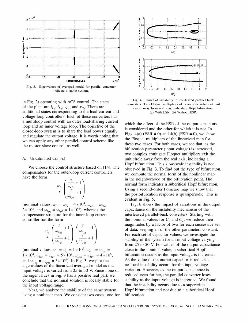
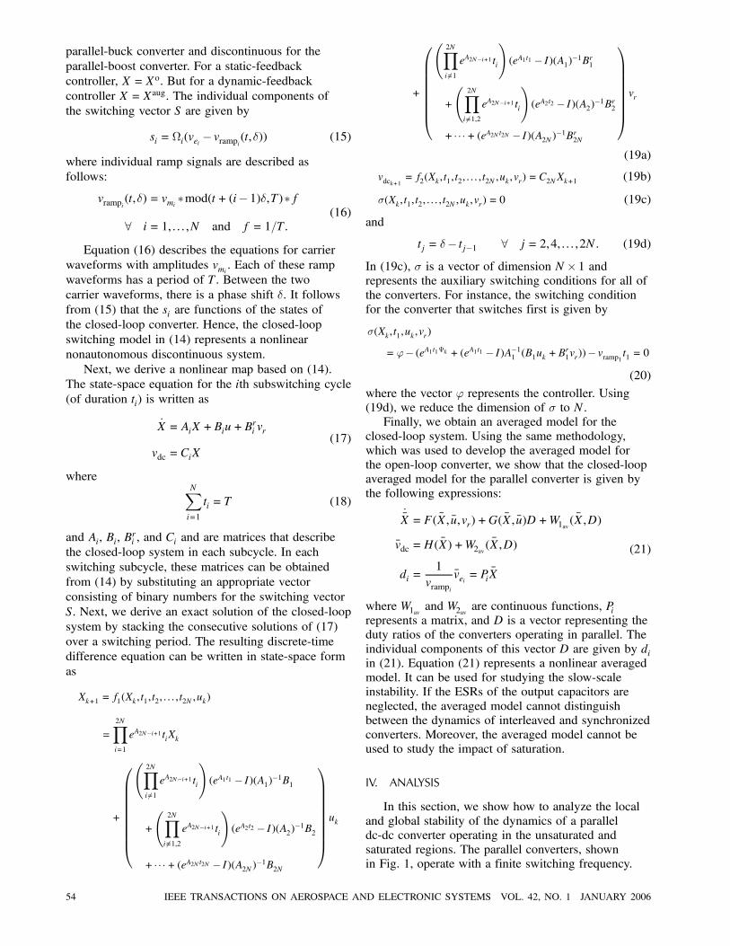
Fig. 3. Eigenvalues of averaged model for parallel converterindicate a stable system.

in Fig. 2) operating with ACS control. The statesof the plant are iL1 , iL2 , vC1 , and vC2 . There areadditional states corresponding to the load-current andvoltage-loop controllers. Each of these converters hasa multiloop control with an outer load-sharing currentloop and an inner voltage loop. The objective of theclosed-loop system is to share the load power equallyand regulate the output voltage. It is worth noting thatwe can apply any other parallel-control scheme likethe master-slave control, as well.

A. Unsaturated Control

We choose the control structure based on [14]. Thecompensators for the outer-loop current controllershave the form

!Iks

0BB@s

!Izk+1

s

!Ipk+1

1CCA(nominal values: !I1 = !I2 = 4 ¤104, !Iz1 = !Iz2 =2 ¤ 103, and !Ip1 = !Ip2 = 1 ¤ 104), whereas thecompensator structure for the inner-loop currentcontroller has the form

!iks

0BB@s

!izk1+1

s

!ipk1+ 1

1CCA0BB@

s

!izk2+1

s

!ipk2+ 1

1CCA(nominal values: !i1 = !i2 = 1 ¤106, !iz11 = !iz21 =1 ¤ 104, !iz12 = !iz22 = 5 ¤ 104, !ip11 = !ip21 = 4 ¤ 105,and !ip12 = !ip22 = 5 ¤105). In Fig. 3, we plot theeigenvalues of the linearized averaged model as theinput voltage is varied from 25 to 50 V. Since none ofthe eigenvalues in Fig. 3 has a positive real part, weconclude that the nominal solution is locally stable forthe input voltage range.Next, we analyze the stability of the same system

using a nonlinear map. We consider two cases: one for

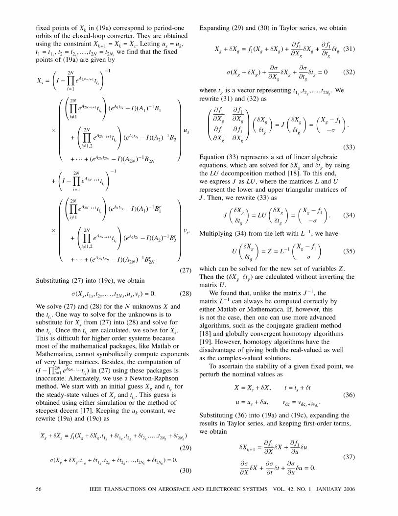
Fig. 4. Onset of instability in interleaved parallel buckconverters. Two Floquet multipliers of period-one orbit exit unit

circle away from real axis, indicating Hopf bifurcation.(a) With ESR. (b) Without ESR.

which the effect of the ESR of the output capacitorsis considered and the other for which it is not. InFigs. 4(a) (ESR 6= 0) and 4(b) (ESR = 0), we showthe Floquet multipliers of the linearized map forthese two cases. For both cases, we see that, as thebifurcation parameter (input voltage) is increased,two complex conjugate Floquet multipliers exit theunit circle away from the real axis, indicating aHopf bifurcation. This slow-scale instability is notobserved in Fig. 3. To find out the type of bifurcation,we compute the normal form of the nonlinear mapin the neighborhood of the bifurcation point. Thenormal form indicates a subcritical Hopf bifurcation.Using a second-order Poincare map we show thatthe postbifurcation response is quasiperiodic. This isevident in Fig. 5.Fig. 6 shows the impact of variations in the output

capacitance on the instability mechanism of theinterleaved parallel-buck converters. Starting withthe nominal values for C1 and C2, we reduce theirmagnitudes by a factor of two for each successive setof data, keeping all of the other parameters constant.For each set of capacitor values, we investigate thestability of the system for an input voltage varyingfrom 25 to 50 V. For values of the output capacitanceclose to the nominal value, a subcritical Hopfbifurcation occurs as the input voltage is increased.As the value of the output capacitor is reduced,no local instability occurs for the input-voltagevariation. However, as the output capacitance isreduced even further, the parallel converter losesstability as the input voltage is increased. We foundthat the instability occurs due to a supercriticalHopf bifurcation and not due to a subcritical Hopfbifurcation.


Fig. 5. Post-Hopf bifurcation scenario of interleaved parallel buck converters. Second-order Poincare map clearly shows quasiperiodicresponse. It shows that even after the onset of instability, voltage ripple magnitude is not drastically large; as such, converter can be

operated close to the boundary, thereby increasing its dynamic response and bandwidth.

Fig. 6. Impact of variations in output capacitance on mechanism of instability of interleaved parallel converters. As capacitance isdecreased, mechanism for instability of parallel converter changes from supercritical to subcritical Hopf bifurcation (ascertained using

the normal in (43)). Subcritical Hopf bifurcation leads to slow-scale instability.

Next, we consider the impact of variations in theinput voltage on the operation of two parallel-buckconverters operating in phase rather than with aphase shift of 180±. We find that, for the samenominal parameters (as considered above), thesynchronized converters are stable for the entireinput voltage range. However, for a higher gain ofthe voltage-loop controller, we observe the onsetof a fast-scale instability with a increasing inputvoltage. The fast-scale instability occurs in the formof a period-doubling bifurcation, as shown in thebifurcation diagram in Fig. 7, which ultimatelyleads to chaos as the input voltage is increasedbeyond 50 V. In Fig. 8, we show the movement ofthe Floquet multipliers of the period-one orbit. Asthe input voltage is increased, one of the Floquetmultipliers exits the unit circle through ¡1, indicatinga period-doubling bifurcation. A second-ordernonlinear map [9] reveals that the period-doublingbifurcation is supercritical in nature.

B. Saturated Control

Finally, we demonstrate the behavior of twoparallel-buck converters operating with a multiloopstatic feedback controller under saturated conditions.We discuss in detail only the cases when bothswitches are turned off. We can extend the sametechnique for the other three cases of full saturation.In a subsequent paper, we will demonstrate howto extend these concepts to converters operatingunder partial saturation and operating with dynamicfeedback controllers. Mazumder, et al. [24] presenta sliding-mode control scheme for parallel-buckand parallel-boost converters that guaranteesstability on all of the hyperplanes and theirintersections.To demonstrate our point, we consider only

the Hamiltonian part of the system. The presenceof the parasitic resistors makes the system morepassive [25, 26]. In addition, we change the controlstrategy from load-current equalization to line-current


Fig. 7. Bifurcation diagram of closed-loop parallel buck converter operating in phase. It shows a fast-scale instability.

Fig. 8. One of the Floquet multipliers of period-one orbit exits the unit circle via ¡1, indicating period-doubling bifurcation.

equalization. For the buck converter, this change doesnot alter the control objectives, which are to regulatethe capacitor voltage and share the load powerequally. However, with these two simple changes, weprove our point more easily.For the closed-loop parallel converter operating

with static-feedback controllers, the switches S1 andS2 are turned off if the error signals of the controllerare less than zero. In this continuity region, the errorsignals are given by

¾k = gvk

0@vr¡fv1vCk + gikfik0@12

2Xj=1

iLj ¡ iLk

1A1A ,k = 1,2: (60)

In (60), fvk are the feedback-sensor gains for theoutput voltages, fik are the feedback-sensor gains forthe inductor currents, gvk and gik are the voltage- andcurrent-loop gains of the two buck-converter modules.We choose the following Lyapunov function in thecontinuity region:

V(¾1,¾2) =12¾

TD¾ = 12(¾1 ¾2)

µ1 0

0 1

¶(¾1 ¾2)

T:

(61)

Therefore,

_V(¾1,¾2) = gv1

Ãvr ¡fv1vC1 + gi1fi1

Ã12

2Xj=1

iLj ¡ iL1

!!

£µgv1gi1fi12

(_iL2 ¡ _iL1 )¡ gv1fv1 _vC1¶

+ gv2

Ãvr ¡fv2vC2 + gi2fi2

Ã12

2Xj=1

iLj ¡ iL2

!!

£µgv2gi2fi22

(_iL1 ¡ _iL2 )¡ gv2fv2 _vC2¶: (62)

Using the constraint vC1 = vC2 = vC , the equations forthe Hamiltonian system

_iLk =¡vCLk+Sku

Lk, 8 k = 1,2 (63a)

_vC =2Xj=1

iLjC1 +C2

¡ vC(C1 +C2)R

(63b)

and assuming S1 = S2 = 0 and gains of the twomodules are the same for simplicity (i.e., gi1 = gi2 = gi,gv1 = gv2 = gv, fi1 = fi2 = fi, and fv1 = fv2 = fv), we


Fig. 9. Stability analysis, based on unsaturated model, predicts a stable equilibrium before and after feedforward disturbance. However,during transients, system saturates. As a result, existence condition _V(¾1,¾2)< 0 is violated. Although error trajectories return back tosliding manifold (as predicted and as illustrated in (b) by switching states that are sampled once in every switching cycle), transientperformance is unacceptable. Part (c) is expansion of transient region in (a) and (b). We note that, in a practical converter, the

fault-protection mechanism will shut down the converter because of large current swings. In other words, the above result demonstratesthat stability alone does not guarantee performance [24].

obtain

_V(¾1,¾2)(S1 = S2 = 0)

=2g2v fvC1 +C2

(vr¡fvvC)³vCR¡ iL1 ¡ iL2

´+g2v g

2i fi2

µ1L1¡ 1L2

¶(iL2 ¡ iL1 )vC: (64)

When the two modules have the same parameters,the second term in (64) vanishes. Using (64), we canshow that when the two converters have the sameparameters, the error trajectories in the continuityregion, given by S1 = S2 = 0, will move toward theboundary layer provided that (vC=R)> iL1 + iL2 . Now,the closed-loop parallel converter (with the sameparameters) operates in the saturated region given byS1 = S2 = 0 only if vr > fvvC. However, the equilibriumsolutions of (63) when S1 = S2 = 0 are iL1 = iL2 = 0and vC = 0. Therefore, the equilibrium solution isvirtual. In other words, the closed-loop converter

cannot remain in this saturated regionpermanently.Next, we consider two cases to demonstrate

these two points. First, we consider a parallel-buckconverter with C1 = C2 = 4400 ¹F and L1 = L2 =50 ¹H. For the second case, we change only the valueof the output capacitor to 100 ¹F. We find that the(unsaturated) nominal solution of the converter incase one is stable for an input voltage range of 70 V,starting at 20 V. The converter in the second casehas a stable (unsaturated) nominal solution at 20 V.However, the nominal solution is unstable at 90 V. Letus assume that initially these converters are operatingin steady state with an input voltage of 20 V. Wethen subject them to a feedforward disturbance sothat the final input voltage is 90 V. The disturbanceis deliberately chosen to be strong enough so thatthe two switches turn off. In other words, S1 = 0 andS2 = 0.Fig. 9 shows the results for case one. We see that

the converter is stable before and after the feedforward


Fig. 10. Stability analysis which predicts that, while the parallel converter is stable before the disturbance, the postdisturbancedynamics are unstable. Inside, there is chaotic attractor inside the boundary layer (which is clearly illustrated in (b) by switching states

that never stabilize). Part (c) is an expansion of (a) and (b) in the region immediately after the disturbance.

disturbance. We predicted this based on the reachingcondition and the stability of the (unsaturated)equilibrium solution. After the disturbance, whenthe system saturates, _V(¾1,¾2) becomes positivebecause (vC=R)> iL1 + iL2 . As a result, the errortrajectories move away from the boundary layer. Sincethe equilibrium solution in the saturated region isvirtual, the error trajectories approach the boundarylayer when _V(¾1,¾2) is less than zero, and eventuallymodulation begins. The states of the system indicatea damped oscillatory behavior before settling downbecause the nominal solution is a stable focus.3

Fig. 10 shows the results for case two. It showsthat, while the parallel converter is stable beforethe disturbance, the postdisturbance dynamics are

3We note that in a practical converter, the system will shutdown dueto fault protection well before the currents attain the large values inFig. 9.

unstable. We know that the error trajectories cannotstay in the saturated region given by S1 = 0 andS2 = 0. However, inside the boundary layer, insteadof a stable nominal solution, we have a chaoticattractor. Hence the dynamics of the converter afterthe disturbance are chaotic. The switching function inFig. 10(b) confirms this. We also see from Fig. 10(c)that the derivative of the Lyapunov function correctlypredicts the dynamics of the error trajectories.We make two observation based on the results of

cases one and two. First, for the same feedforwarddisturbance, the derivative of the Lyapunov functionfor case two spends much less time in the saturatedregion as compared with+ case one. This is because,for the second case, the voltage across the capacitor(for a given load), due of its smaller size, changesmore rapidly with changes in the inductor current. Wecan verify this by neglecting the second term in (64).Second, although a reduction in the capacitance gives


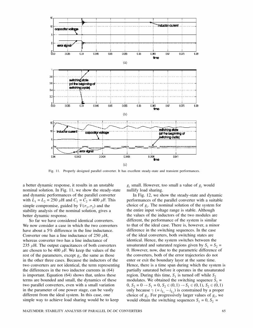
Fig. 11. Properly designed parallel converter. It has excellent steady-state and transient performances.

a better dynamic response, it results in an unstablenominal solution. In Fig. 11, we show the steady-stateand dynamic performances of the parallel converterwith L1 = L2 = 250 ¹H and C1 = C2 = 400 ¹F. Thissimple compromise, guided by _V(¾1,¾2) and thestability analysis of the nominal solution, gives abetter dynamic response.So far we have considered identical converters.

We now consider a case in which the two convertershave about a 5% difference in the line inductance.Converter one has a line inductance of 250 ¹H,whereas converter two has a line inductance of235 ¹H. The output capacitances of both convertersare chosen to be 400 ¹F. We keep the values of therest of the parameters, except gi, the same as thosein the other three cases. Because the inductors of thetwo converters are not identical, the term representingthe differences in the two inductor currents in (64)is important. Equation (64) shows that, unless theseterms are bounded and small, the dynamics of thesetwo parallel converters, even with a small variationin the parameter of one power stage, can be vastlydifferent from the ideal system. In this case, onesimple way to achieve load sharing would be to keep

gi small. However, too small a value of gi wouldnullify load sharing.In Fig. 12, we show the steady-state and dynamic

performances of the parallel converter with a suitablechoice of gi. The nominal solution of the system forthe entire input voltage range is stable. Althoughthe values of the inductors of the two modules aredifferent, the performance of the system is similarto that of the ideal case. There is, however, a minordifference in the switching sequences. In the caseof the ideal converters, both switching states areidentical. Hence, the system switches between theunsaturated and saturated regions given by S1 = S2 =0. However, now, due to the parametric difference ofthe converters, both of the error trajectories do notenter or exit the boundary layer at the same time.Hence, there is a time span during which the system ispartially saturated before it operates in the unsaturatedregion. During this time, S1 is turned off while S2modulates. We obtained the switching sequence S1 =0, S2 = 0! S1 = 0, S2 2 (0,1)! S1 2 (0,1), S2 2 (0,1)only because ° (= iL1 ¡ iL2 ) is constrained by a properchoice of gi. For progressively larger values of gi, wewould obtain the switching sequences S1 = 0, S2 =


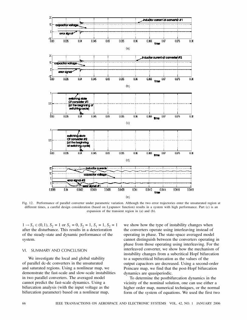
Fig. 12. Performance of parallel converter under parametric variation. Although the two error trajectories enter the unsaturated region atdifferent times, a careful design consideration (based on Lyapunov function) results in a system with high performance. Part (c) is an

expansion of the transient region in (a) and (b).

1! S1 2 (0,1), S2 = 1 or S1 = 0, S2 = 1, S1 = 1, S2 = 1after the disturbance. This results in a deteriorationof the steady-state and dynamic performance of thesystem.

VI. SUMMARY AND CONCLUSION

We investigate the local and global stabilityof parallel dc-dc converters in the unsaturatedand saturated regions. Using a nonlinear map, wedemonstrate the fast-scale and slow-scale instabilitiesin two parallel converters. The averaged modelcannot predict the fast-scale dynamics. Using abifurcation analysis (with the input voltage as thebifurcation parameter) based on a nonlinear map,

we show how the type of instability changes whenthe converters operate using interleaving instead ofoperating in phase. The state-space averaged modelcannot distinguish between the converters operating inphase from those operating using interleaving. For theinterleaved converter, we show how the mechanism ofinstability changes from a subcritical Hopf bifurcationto a supercritical bifurcation as the values of theoutput capacitors are decreased. Using a second-orderPoincare map, we find that the post-Hopf bifurcationdynamics are quasiperiodic.To determine the postbifurcation dynamics in the

vicinity of the nominal solution, one can use either ahigher order map, numerical techniques, or the normalform of the system of equations. We used the first two


methods for standalone converters [9]. Because thedimensionality of the closed-loop parallel converter is,in general, higher than that of standalone converters,the normal form may be a better alternative. In thispaper, we have outlined a technique to generate thenormal form of a closed-loop system described by anonlinear map. We will discuss this methodology, indetail, in another paper.We also outline ways to determine the stability

of saturated regions, which we demonstrate usingtwo synchronized parallel buck converters. Using apositive definite Lyapunov function, we show that,for a fully saturated parallel converter, the dynamicsof the system in the saturated region are governedby the derivative of the Lyapunov function. Whenthe derivative of the Lyapunov function is negative,the error trajectories approach the boundary layer.When the derivative is positive, the error trajectoriesleave the saturated region. In this case, we show thatif the equilibrium solutions of the saturated regionsare virtual, these trajectories will ultimately reach theboundary layer.Finally, we apply these concepts of stability

for the saturated and unsaturated regions to fourcases. For the first three cases, we consider theparameters of the parallel converters to be thesame. We show, using cases one and two, that thenominal solution (in the unsaturated region) isstable if and only if the dynamics of the system inthe saturated and unsaturated regions are stable.That is why, while the postdisturbance steady-statedynamics of the closed-loop system in case oneare stable, they are chaotic for the second case.However, we find that the transient dynamics forcase one are much more oscillatory than those ofcase two. We explain this using the derivative ofthe Lyapunov function. Based on these two cases,we show in case three how easily one can improvethe transient and steady-state performances of thesystem. For the fourth case, we consider two parallelbuck converters with parametric variation. Using(64), we show how to tune the outer-loop currentgain gi so that the performance of the nonidealsystem is close to the ideal case. We also showhow and why the switching sequence changes withincreasing gi.

APPENDIX A. AVERAGE MODEL FOR TWOPARALLEL BUCK CONVERTERS

In each switching cycle (of duration T), thereare four subintervals (see Fig. 13). The switchingsequence in each switching cycle is S1 = 1, S2 =0! S1 = 0, S2 = 0! S1 = 0, S2 = 1! S1 = 0, S2 =0. Using (4), we obtain the following state-space

Fig. 13. Interleaved converters.

Fig. 14. Synchronized (in-phase) converters.

equations for these four subintervals:

_Xo = Ao10Xo +Bo10u, t < t1

_Xo = Ao00Xo +Bo00u, t1 < t < t1 + t2

_Xo = Ao01Xo +Bo01u, t1 + t2 < t < t1 + t2 + t3

_Xo = Ao00Xo +Bo00u, t1 + t2 + t3 < t < T:

(65)

For the dc-dc buck converter, Ao10 = Ao00 = A

o01 = A

o

and Bo00 = 0. Averaging the four equations in (65)yields

_Xo = AoXo +³ t1TBo10 +

t3TBo01

´u: (66)

The duty ratio for the two buck converters of theparallel module are defined by d1 = t1=T and d2 =t3=T, respectively. Rewriting (66) in terms of d1 andd2, one obtains the following averaged model:

_Xo = AoXo + (d1Bo10 + d2B

o01)u: (67)

In each switching cycle (of duration T), there are foursubintervals (see Fig. 14). The switching sequence ineach switching cycle is S1 = 1, S2 = 1! S1 = 0, S2 =1! S1 = 0, S2 = 0. Using (4), we obtain the followingstate-space equations for these three subintervals:

_Xo = Ao11Xo +Bo11u, t < t1

_Xo = Ao01Xo +Bo01u, t1 < t < t1 + t2

_Xo = Ao00Xo +Bo00u, t1 + t2 < t < T:

(68)


For the dc-dc buck converter, Ao11 = Ao01 = A

o00 = A

o

and Bo00 = 0. Averaging the three equations in (68)yields

_Xo = AoXo +³ t1TBo11 +

t1 + t2T

Bo01

´u: (69)

The duty ratio for the two buck converters of theparallel module are defined by d1 = t1=T and d2 =(t1 + t2)=T, respectively. Rewriting (69) in terms ofd1 and d2, one obtains the following averaged model:

_Xo = AoXo + (d1Bo11 + d2B

o01)u: (70)

REFERENCES

[1] Nayfeh, A. H., and Balachandran, B.Applied Nonlinear Dynamics.New York: Wiley, 1995.

[2] Khalil, H. K.Nonlinear Systems.Englewood Cliffs, NJ: Prentice-Hall, 1996.

[3] Aubin, J., and Cellina, A.Differential Inclusions: Set-Valued Maps and ViabilityTheory.New York: Springer-Verlag, 1984.

[4] Filippov, A. F.Differential Equations with Discontinuous Righthand Sides.Boston, Kluwer, 1988.

[5] Utkin, V.Sliding Modes in Control Optimization.New York: Springer-Verlag, 1992.

[6] Deane, J. H. B., and Hamill, D. C.Analysis, simulation and experimental study of chaos inthe buck converter.In Proceedings of IEEE Power Electronics SpecialistsConference, 1990, 491—498.

[7] Tse, C. K.Flip bifurcation and chaos in three-state boost switchingregulators.IEEE Transactions on Circuits and Systems-1: FundamentalTheory and Applications, 41 (1994), 16—23.

[8] Banerjee, S., Ott, E., Yorke, J. A., and Yuan, G. H.Anomalous bifurcations in dc-dc converters: Borderlinecollisions in piecewise smooth maps.In Proceedings of IEEE Power Electronic SpecialistsConference, 1997, 1337—1344.

[9] Mazumder, S. K., Nayfeh, A. H., and Boroyevich, D.A theoretical and experimental investigation of the fast-and slow-scale instabilities of a dc-dc converter.IEEE Transactions on Power Electronics, 16, 2 (2001),201—216.

[10] Middlebrook, R. D., and Cuk, S.A general unified approach to modelingswitching-converter power stages.In Proceedings of IEEE Power Electronic SpecialistsConference, 1977, 521—550.

[11] Lee, F. C.Modeling, Analysis, and Design of PWM Converter.Virginia Power Electronic Center Publications Series,vol. 2, Blacksburg, VA, 1990.

[12] Rajagopalan, J., Xing, K., Guo, and Lee, F. C.Modeling and dynamic analysis of paralleled dc/dcconverters with master/slave current sharing control.In Proceedings of IEEE Applied Power ElectronicsConference, 1996, 678—684.

[13] Kohama, T., Ninomiya, T., Shoyama, M., Ihara, F.Dynamic analysis of parallel-module converter systemwith current balance controllers.In Proceedings of International Telecommunications EnergyConference, 1994, 190—195.

[14] Thottuvelli, V. J., and Verghese, G. C.Stability analysis of paralleled dc/dc converters withactive current sharing.In Proceedings of IEEE Power Electronics SpecialistsConference, 1996, 1080—1086.

[15] Parker, T. S., and Chua, L. O.Practical Numerical Algorithms for Chaotic Systems.New York: Springer-Verlag, 1989.

[16] Royden, H. L.Real Analysis.Englewood Cliffs, NJ: Prentice-Hall, 1988.

[17] Dennis, J. E., Jr., and Schnabel, R. B.Numerical Methods for Unconstrained Optimization andNonlinear Equations.Englewood Cliffs, NJ: Prentice-Hall, 1983.

[18] Salon, S. J.Computer Methods in Electrical Power Engineering.Dept. of Electrical Power Engineering, RensselaerPolytechnic Institute, Troy, NY, Class notes, 1993.

[19] Watson, L. T.Globally convergent homotopy algorithms for nonlinearsystems of equations.Nonlinear Dynamics, 1 (1990), 143—191.

[20] Brogliato, B.Nonsmooth Impact Mechanics: Models, Dynamics andControl.New York: Springer-Verlag, 1996.

[21] Nayfeh, A. H.Method of Normal Forms.New York: Wiley Interscience, 1993.

[22] Shevitz, D., and Paden, B.Lyapunov stability theory of nonsmooth systems.IEEE Transactions on Automatic Control, 39 (1994),1910—1914.

[23] Wu, Q., Onyshko, S., Sepehri, N., and Thornton-Trump,A. B.On construction of smooth Lyapunov functions fornon-smooth systems.International Journal of Control, 69 (1998), 443—457.

[24] Mazumder, S. K., Nayfeh, A. H., and Boroyevich, D.Robust control of parallel dc-dc buck convertersby combining integral-variable structure andmultiple-sliding-surface control schemes.IEEE Transactions on Power Electronics, 17, 3 (2002),428—437.

[25] Sanders, S.Nonlinear control of switching power converters.Ph.D. dissertation, Dept. of Electrical and ComputerEngineering, Massachusetts Institute of Technology,Cambridge, MA, 1989.

[26] van der Schaft, A. J.L2-Gain and Passivity Techniques in Nonlinear Control.New York: Springer, 1996.

[27] Siri, K.Analysis and design of distributed power systems.Ph.D. dissertation, Dept. of Electrical Engineering,University of Illinois at Chicago, IL, 1991.

[28] Siri, K., Lee, C. Q., and Wu, T. F.Current distribution control for parallel-connectedconverters.IEEE Transactions on Aerospace and Electronic Systems,28, 3 (1992), 829—850.


[29] Panov, Y., and Jovanovic, M. M.Stability and dynamic performance of current-sharingcontrol of paralleled voltage regulator modules.IEEE Transactions on Power Electronics, 17, 2 (2002),172—179.

[30] Abu-Qahouq, J. A., Hong Mao, and Batarseh, I.Novel control method for multiphase low-voltagehigh-current fast-transient VRMs.In Proceedings of IEEE Power Electronics SpecialistsConference, 2002, 1576—1581.

[31] Mazumder, S. K,. and Nayfeh, A. H.A new approach to the stability analysis of boostpower-factor-correction circuits.Journal of Vibrations and Control, Special Issue onNonlinear Controls and Dynamics, 9 (2003), 749—773.

Sudip K. Mazumder (M’01–SM’04) is the Director of Laboratory for Energyand Switching-Electronics Systems (LESES) and an assistant professor in theDepartment of Electrical and Computer Engineering at the University of Illinois,Chicago. He received his Ph.D. and M.S. degrees from Virginia PolytechnicInstitute and State University, Blacksburg, Virginia and Rensselaer PolytechnicInstitute, Troy, New York, in 2001 and 1993, respectively. He has over 10years of professional experience and has held R&D and design positions inleading industrial organizations. His current areas of interests are interactivepower-electronics/power networks, renewable and alternate energy systems, andnew device and systems-on-chip enabled higher power density.Dr. Mazumder received the ONR Young Investigator Award, NSF CAREER,

and the DOE SECA awards in 2005, 2003, and 2002, respectively. He alsoreceived the Prize Paper Award from the IEEE Transactions on Power Electronicsand the IEEE PELS in 2002. He is an associate editor for the IEEE Transactionson Industrial Electronics and IEEE Power Electronics Letters. He has publishedover 50 refereed and invited journal and conference papers and is a reviewer for 6international journals.

[32] Mazumder, S. K., Nayfeh, A. H., and Boroyevich, D.A nonlinear approach to the analysis of stability anddynamics of standalone and parallel dc-dc converters.Annual Proceedings of the Center for Power ElectronicsSystems, (2000), 610—616. Also in Stability analysis ofparallel dc-dc converters using a nonlinear approach.IEEE Power Electronics Specialists Conference, 2001,1283—1288.

[33] Iu, H. H. C., and Tse, C. K.Bifurcation behavior in parallel-connected buckconverters.IEEE Transactions on Circuits and Systems I, 48 (2002),233—240.


Stability Analysis of Parallel DC-DC Converters - …mazumder/14.pdf · Stability Analysis of...

Documents

Transcript of Stability Analysis of Parallel DC-DC Converters - …mazumder/14.pdf · Stability Analysis of...