Springer Undergraduate Mathematics Seriesbrusso/ErdWilLieAlg254pp.pdf · 2017-04-16 · Measure,...

Springer Undergraduate Mathematics Series

Advisory Board

M.A.J. Chaplain University of DundeeK. Erdmann Oxford UniversityA.MacIntyre Queen Mary, University of LondonL.C.G. Rogers University of CambridgeE. Süli Oxford UniversityJ.F. Toland University of Bath

Other books in this series

A First Course in Discrete Mathematics I. AndersonAnalytic Methods for Partial Differential Equations G. Evans, J. Blackledge, P. YardleyApplied Geometry for Computer Graphics and CAD, Second Edition D. MarshBasic Linear Algebra, Second Edition T.S. Blyth and E.F. RobertsonBasic Stochastic Processes Z. Brzezniak and T. ZastawniakCalculus of One Variable K.E. HirstComplex Analysis J.M. HowieElementary Differential Geometry A. PressleyElementary Number Theory G.A. Jones and J.M. JonesElements of Abstract Analysis M. Ó SearcóidElements of Logic via Numbers and Sets D.L. JohnsonEssential Mathematical Biology N.F. BrittonEssential Topology M.D. CrossleyFields and Galois Theory J.M. HowieFields, Flows and Waves: An Introduction to Continuum Models D.F. ParkerFurther Linear Algebra T.S. Blyth and E.F. RobertsonGeometry R. FennGroups, Rings and Fields D.A.R. WallaceHyperbolic Geometry, Second Edition J.W. AndersonInformation and Coding Theory G.A. Jones and J.M. JonesIntroduction to Laplace Transforms and Fourier Series P.P.G. DykeIntroduction to Lie Algebras K. Erdmann and M.J. WildonIntroduction to Ring Theory P.M. CohnIntroductory Mathematics: Algebra and Analysis G. SmithLinear Functional Analysis B.P. Rynne and M.A. YoungsonMathematics for Finance: An Introduction to Financial Engineering M. Capinksi

and T. ZastawniakMatrix Groups: An Introduction to Lie Group Theory A. BakerMeasure, Integral and Probability, Second Edition M. Capinksi and E. KoppMultivariate Calculus and Geometry, Second Edition S. DineenNumerical Methods for Partial Differential Equations G. Evans, J. Blackledge,

P. YardleyProbability Models J.HaighReal Analysis J.M. HowieSets, Logic and Categories P. CameronSpecial Relativity N.M.J. WoodhouseSymmetries D.L. JohnsonTopics in Group Theory G. Smith and O. TabachnikovaVector Calculus P.C. Matthews

Karin Erdmann and Mark J. Wildon

Introduction toLie Algebras

Karin ErdmannMathematical Institute24–29 St Giles’Oxford OX1 [email protected]

Mark J. WildonMathematical Institute24–29 St Giles’Oxford OX1 [email protected]

British Library Cataloguing in Publication DataA catalogue record for this book is available from the British Library

Library of Congress Control Number: 2005937687

Springer Undergraduate Mathematics Series ISSN 1615-2085

Printed on acid-free paper

Apart from any fair dealing for the purposes of research or private study, or criticism or review, as permitted under the Copyright, Designs and Patents Act 1988, this publication may only be reproduced, stored or transmitted, in any form or by any means, with the prior permission in writing of the publishers, or in the case of reprographic reproduction in accordance with the terms of licences issued by the Copyright Licensing Agency. Enquiries concerning reproduction outside those terms should be sent to the publishers.

The use of registered names, trademarks, etc., in this publication does not imply, even in the absence of a specifi c statement, that such names are exempt from the relevant laws and regulations andfitherefore free for general use.

The publisher makes no representation, express or implied, with regard to the accuracy of the information contained in this book and cannot accept any legal responsibility or liability for any errors or omissions that may be made.

(corrected as of 2nd printing, 2007)

Springer Science+Business Media

9 8 7 6 5 4 3 2

© Springer-Verlag LVV ondon Limited 2006

springer.com

ISBN 978-1-84628-040-5 ISBN 978-1-84628-490-8 (eBook)DOI 10.1007/978-1-84628-490-8

Preface

Lie theory has its roots in the work of Sophus Lie, who studied certain trans-formation groups that are now called Lie groups. His work led to the discoveryof Lie algebras. By now, both Lie groups and Lie algebras have become essen-tial to many parts of mathematics and theoretical physics. In the meantime,Lie algebras have become a central object of interest in their own right, notleast because of their description by the Serre relations, whose generalisationshave been very important.

This text aims to give a very basic algebraic introduction to Lie algebras.We begin here by mentioning that “Lie” should be pronounced “lee”. Theonly prerequisite is some linear algebra; we try throughout to be as simple aspossible, and make no attempt at full generality. We start with fundamentalconcepts, including ideals and homomorphisms. A section on Lie algebras ofsmall dimension provides a useful source of examples. We then define solvableand simple Lie algebras and give a rough strategy towards the classification ofthe finite-dimensional complex Lie algebras. The next chapters discuss Engel’sTheorem, Lie’s Theorem, and Cartan’s Criteria and introduce some represen-tation theory.

We then describe the root space decomposition of a semisimple Lie alge-bra and introduce Dynkin diagrams to classify the possible root systems. Topractice these ideas, we find the root space decompositions of the classical Liealgebras. We then outline the remarkable classification of the finite-dimensionalsimple Lie algebras over the complex numbers.

The final chapter is a survey on further directions. In the first part, weintroduce the universal enveloping algebra of a Lie algebra and look in more

vi Preface

detail at representations of Lie algebras. We then look at the Serre relationsand their generalisations to Kac–Moody Lie algebras and quantum groups anddescribe the Lie ring associated to a group. In fact, Dynkin diagrams and theclassification of the finite-dimensional complex semisimple Lie algebras havehad a far-reaching influence on modern mathematics; we end by giving anillustration of this.

In Appendix A, we give a summary of the basic linear and bilinear alge-bra we need. Some technical proofs are deferred to Appendices B, C, and D.In Appendix E, we give answers to some selected exercises. We do, however,encourage the reader to make a thorough unaided attempt at these exercises:it is only when treated in this way that they will be of any benefit. Exercisesare marked † if an answer may be found in Appendix E and � if they are eithersomewhat harder than average or go beyond the usual scope of the text.

University of Oxford Karin ErdmannJanuary 2006 Mark Wildon

Contents

Preface . . . . . . . . . . . . . . . . . . . . . . . . . . . . . . . . . . . . . . . . . . . . . . . . . . . . . v

1. Introduction . . . . . . . . . . . . . . . . . . . . . . . . . . . . . . . . . . . . . . . . . . . . . . . . 11.1 Definition of Lie Algebras . . . . . . . . . . . . . . . . . . . . . . . . . . . . . . . . . 11.2 Some Examples . . . . . . . . . . . . . . . . . . . . . . . . . . . . . . . . . . . . . . . . . . 21.3 Subalgebras and Ideals . . . . . . . . . . . . . . . . . . . . . . . . . . . . . . . . . . . . 31.4 Homomorphisms . . . . . . . . . . . . . . . . . . . . . . . . . . . . . . . . . . . . . . . . . 41.5 Algebras . . . . . . . . . . . . . . . . . . . . . . . . . . . . . . . . . . . . . . . . . . . . . . . . 51.6 Derivations . . . . . . . . . . . . . . . . . . . . . . . . . . . . . . . . . . . . . . . . . . . . . . 61.7 Structure Constants . . . . . . . . . . . . . . . . . . . . . . . . . . . . . . . . . . . . . . 7

2. Ideals and Homomorphisms . . . . . . . . . . . . . . . . . . . . . . . . . . . . . . . . 112.1 Constructions with Ideals . . . . . . . . . . . . . . . . . . . . . . . . . . . . . . . . . . 112.2 Quotient Algebras . . . . . . . . . . . . . . . . . . . . . . . . . . . . . . . . . . . . . . . 122.3 Correspondence between Ideals . . . . . . . . . . . . . . . . . . . . . . . . . . . . . 14

3. Low-Dimensional Lie Algebras . . . . . . . . . . . . . . . . . . . . . . . . . . . . . . 193.1 Dimensions 1 and 2 . . . . . . . . . . . . . . . . . . . . . . . . . . . . . . . . . . . . . . . 203.2 Dimension 3 . . . . . . . . . . . . . . . . . . . . . . . . . . . . . . . . . . . . . . . . . . . . . 20

4. Solvable Lie Algebras and a Rough Classification . . . . . . . . . . . 274.1 Solvable Lie Algebras . . . . . . . . . . . . . . . . . . . . . . . . . . . . . . . . . . . . . 274.2 Nilpotent Lie Algebras . . . . . . . . . . . . . . . . . . . . . . . . . . . . . . . . . . . . 314.3 A Look Ahead . . . . . . . . . . . . . . . . . . . . . . . . . . . . . . . . . . . . . . . . . . . 32

viii Contents

5. Subalgebras of gl(V ) . . . . . . . . . . . . . . . . . . . . . . . . . . . . . . . . . . . . . . . . 375.1 Nilpotent Maps . . . . . . . . . . . . . . . . . . . . . . . . . . . . . . . . . . . . . . . . . . 375.2 Weights . . . . . . . . . . . . . . . . . . . . . . . . . . . . . . . . . . . . . . . . . . . . . . . . . 385.3 The Invariance Lemma . . . . . . . . . . . . . . . . . . . . . . . . . . . . . . . . . . . . 395.4 An Application of the Invariance Lemma . . . . . . . . . . . . . . . . . . . . 42

6. Engel’s Theorem and Lie’s Theorem . . . . . . . . . . . . . . . . . . . . . . . . 456.1 Engel’s Theorem . . . . . . . . . . . . . . . . . . . . . . . . . . . . . . . . . . . . . . . . . 466.2 Proof of Engel’s Theorem. . . . . . . . . . . . . . . . . . . . . . . . . . . . . . . . . . 486.3 Another Point of View . . . . . . . . . . . . . . . . . . . . . . . . . . . . . . . . . . . . 486.4 Lie’s Theorem. . . . . . . . . . . . . . . . . . . . . . . . . . . . . . . . . . . . . . . . . . . . 49

7. Some Representation Theory . . . . . . . . . . . . . . . . . . . . . . . . . . . . . . . 537.1 Definitions . . . . . . . . . . . . . . . . . . . . . . . . . . . . . . . . . . . . . . . . . . . . . . . 537.2 Examples of Representations . . . . . . . . . . . . . . . . . . . . . . . . . . . . . . . 547.3 Modules for Lie Algebras . . . . . . . . . . . . . . . . . . . . . . . . . . . . . . . . . . 557.4 Submodules and Factor Modules . . . . . . . . . . . . . . . . . . . . . . . . . . . 577.5 Irreducible and Indecomposable Modules . . . . . . . . . . . . . . . . . . . . 587.6 Homomorphisms . . . . . . . . . . . . . . . . . . . . . . . . . . . . . . . . . . . . . . . . . 607.7 Schur’s Lemma . . . . . . . . . . . . . . . . . . . . . . . . . . . . . . . . . . . . . . . . . . . 61

8. Representations of sl(2, C) . . . . . . . . . . . . . . . . . . . . . . . . . . . . . . . . . . 678.1 The Modules Vd . . . . . . . . . . . . . . . . . . . . . . . . . . . . . . . . . . . . . . . . . . 678.2 Classifying the Irreducible sl(2,C)-Modules . . . . . . . . . . . . . . . . . . 718.3 Weyl’s Theorem . . . . . . . . . . . . . . . . . . . . . . . . . . . . . . . . . . . . . . . . . . 74

9. Cartan’s Criteria . . . . . . . . . . . . . . . . . . . . . . . . . . . . . . . . . . . . . . . . . . . 779.1 Jordan Decomposition . . . . . . . . . . . . . . . . . . . . . . . . . . . . . . . . . . . . 779.2 Testing for Solvability . . . . . . . . . . . . . . . . . . . . . . . . . . . . . . . . . . . . . 789.3 The Killing Form . . . . . . . . . . . . . . . . . . . . . . . . . . . . . . . . . . . . . . . . . 809.4 Testing for Semisimplicity . . . . . . . . . . . . . . . . . . . . . . . . . . . . . . . . . 819.5 Derivations of Semisimple Lie Algebras . . . . . . . . . . . . . . . . . . . . . . 849.6 Abstract Jordan Decomposition . . . . . . . . . . . . . . . . . . . . . . . . . . . . 85

10. The Root Space Decomposition . . . . . . . . . . . . . . . . . . . . . . . . . . . . . 9110.1 Preliminary Results . . . . . . . . . . . . . . . . . . . . . . . . . . . . . . . . . . . . . . . 9210.2 Cartan Subalgebras . . . . . . . . . . . . . . . . . . . . . . . . . . . . . . . . . . . . . . 9510.3 Definition of the Root Space Decomposition . . . . . . . . . . . . . . . . . 9710.4 Subalgebras Isomorphic to sl(2,C) . . . . . . . . . . . . . . . . . . . . . . . . . . 9710.5 Root Strings and Eigenvalues . . . . . . . . . . . . . . . . . . . . . . . . . . . . . . 9910.6 Cartan Subalgebras as Inner-Product Spaces . . . . . . . . . . . . . . . . . 102

Contents ix

11. Root Systems . . . . . . . . . . . . . . . . . . . . . . . . . . . . . . . . . . . . . . . . . . . . . . . 10911.1 Definition of Root Systems . . . . . . . . . . . . . . . . . . . . . . . . . . . . . . . . 10911.2 First Steps in the Classification . . . . . . . . . . . . . . . . . . . . . . . . . . . . 11111.3 Bases for Root Systems . . . . . . . . . . . . . . . . . . . . . . . . . . . . . . . . . . . 11511.4 Cartan Matrices and Dynkin Diagrams . . . . . . . . . . . . . . . . . . . . . . 120

12. The Classical Lie Algebras . . . . . . . . . . . . . . . . . . . . . . . . . . . . . . . . . . 12512.1 General Strategy . . . . . . . . . . . . . . . . . . . . . . . . . . . . . . . . . . . . . . . . . 12612.2 sl(� + 1,C) . . . . . . . . . . . . . . . . . . . . . . . . . . . . . . . . . . . . . . . . . . . . . . 12912.3 so(2� + 1,C) . . . . . . . . . . . . . . . . . . . . . . . . . . . . . . . . . . . . . . . . . . . . . 13012.4 so(2�,C) . . . . . . . . . . . . . . . . . . . . . . . . . . . . . . . . . . . . . . . . . . . . . . . . 13312.5 sp(2�,C) . . . . . . . . . . . . . . . . . . . . . . . . . . . . . . . . . . . . . . . . . . . . . . . . 13412.6 Killing Forms of the Classical Lie Algebras . . . . . . . . . . . . . . . . . . 13612.7 Root Systems and Isomorphisms . . . . . . . . . . . . . . . . . . . . . . . . . . . 137

13. The Classification of Root Systems . . . . . . . . . . . . . . . . . . . . . . . . . 14113.1 Classification of Dynkin Diagrams . . . . . . . . . . . . . . . . . . . . . . . . . . 14213.2 Constructions . . . . . . . . . . . . . . . . . . . . . . . . . . . . . . . . . . . . . . . . . . . . 148

14. Simple Lie Algebras . . . . . . . . . . . . . . . . . . . . . . . . . . . . . . . . . . . . . . . . 15314.1 Serre’s Theorem . . . . . . . . . . . . . . . . . . . . . . . . . . . . . . . . . . . . . . . . . . 15414.2 On the Proof of Serre’s Theorem . . . . . . . . . . . . . . . . . . . . . . . . . . . 15814.3 Conclusion . . . . . . . . . . . . . . . . . . . . . . . . . . . . . . . . . . . . . . . . . . . . . . 160

15. Further Directions . . . . . . . . . . . . . . . . . . . . . . . . . . . . . . . . . . . . . . . . . . 16315.1 The Irreducible Representations of a Semisimple Lie Algebra . . . 16415.2 Universal Enveloping Algebras . . . . . . . . . . . . . . . . . . . . . . . . . . . . . 17115.3 Groups of Lie Type . . . . . . . . . . . . . . . . . . . . . . . . . . . . . . . . . . . . . . . 17715.4 Kac–Moody Lie Algebras . . . . . . . . . . . . . . . . . . . . . . . . . . . . . . . . . 17915.5 The Restricted Burnside Problem . . . . . . . . . . . . . . . . . . . . . . . . . . 18015.6 Lie Algebras over Fields of Prime Characteristic . . . . . . . . . . . . . . 18315.7 Quivers . . . . . . . . . . . . . . . . . . . . . . . . . . . . . . . . . . . . . . . . . . . . . . . . . 184

16. Appendix A: Linear Algebra . . . . . . . . . . . . . . . . . . . . . . . . . . . . . . . . 18916.1 Quotient Spaces . . . . . . . . . . . . . . . . . . . . . . . . . . . . . . . . . . . . . . . . . . 18916.2 Linear Maps . . . . . . . . . . . . . . . . . . . . . . . . . . . . . . . . . . . . . . . . . . . . . 19116.3 Matrices and Diagonalisation . . . . . . . . . . . . . . . . . . . . . . . . . . . . . . 19216.4 Interlude: The Diagonal Fallacy . . . . . . . . . . . . . . . . . . . . . . . . . . . . 19716.5 Jordan Canonical Form . . . . . . . . . . . . . . . . . . . . . . . . . . . . . . . . . . . 19816.6 Jordan Decomposition . . . . . . . . . . . . . . . . . . . . . . . . . . . . . . . . . . . . 20016.7 Bilinear Algebra . . . . . . . . . . . . . . . . . . . . . . . . . . . . . . . . . . . . . . . . . . 201

x Contents

17. Appendix B: Weyl’s Theorem . . . . . . . . . . . . . . . . . . . . . . . . . . . . . . 20917.1 Trace Forms . . . . . . . . . . . . . . . . . . . . . . . . . . . . . . . . . . . . . . . . . . . . 20917.2 The Casimir Operator . . . . . . . . . . . . . . . . . . . . . . . . . . . . . . . . . . . . 211

18. Appendix C: Cartan Subalgebras . . . . . . . . . . . . . . . . . . . . . . . . . . . 21518.1 Root Systems of Classical Lie Algebras . . . . . . . . . . . . . . . . . . . . . . 21518.2 Orthogonal and Symplectic Lie Algebras . . . . . . . . . . . . . . . . . . . . 21718.3 Exceptional Lie Algebras . . . . . . . . . . . . . . . . . . . . . . . . . . . . . . . . . . 22018.4 Maximal Toral Subalgebras . . . . . . . . . . . . . . . . . . . . . . . . . . . . . . . 221

19. Appendix D: Weyl Groups . . . . . . . . . . . . . . . . . . . . . . . . . . . . . . . . . . 22319.1 Proof of Existence . . . . . . . . . . . . . . . . . . . . . . . . . . . . . . . . . . . . . . . . 22319.2 Proof of Uniqueness . . . . . . . . . . . . . . . . . . . . . . . . . . . . . . . . . . . . . . 22419.3 Weyl Groups . . . . . . . . . . . . . . . . . . . . . . . . . . . . . . . . . . . . . . . . . . . . . 226

20. Appendix E: Answers to Selected Exercises . . . . . . . . . . . . . . . . . 231

Bibliography . . . . . . . . . . . . . . . . . . . . . . . . . . . . . . . . . . . . . . . . . . . . . . . . . . . . 247

Index . . . . . . . . . . . . . . . . . . . . . . . . . . . . . . . . . . . . . . . . . . . . . . . . . . . . . . . . . . . 249

1Introduction

We begin by defining Lie algebras and giving a collection of typical examplesto which we shall refer throughout this book. The remaining sections in thischapter introduce the basic vocabulary of Lie algebras. The reader is remindedthat the prerequisite linear and bilinear algebra is summarised in Appendix A.

1.1 Definition of Lie Algebras

Let F be a field. A Lie algebra over F is an F -vector space L, together with abilinear map, the Lie bracket

L × L → L, (x, y) �→ [x, y],

satisfying the following properties:

[x, x] = 0 for all x ∈ L, (L1)

[x, [y, z]] + [y, [z, x]] + [z, [x, y]] = 0 for all x, y, z ∈ L. (L2)

The Lie bracket [x, y] is often referred to as the commutator of x and y.Condition (L2) is known as the Jacobi identity. As the Lie bracket [−,−] isbilinear, we have

0 = [x + y, x + y] = [x, x] + [x, y] + [y, x] + [y, y] = [x, y] + [y, x].

Hence condition (L1) implies

[x, y] = −[y, x] for all x, y ∈ L. (L1′)

2 1. Introduction

If the field F does not have characteristic 2, then putting x = y in (L1′) showsthat (L1′) implies (L1).

Unless specifically stated otherwise, all Lie algebras in this book should betaken to be finite-dimensional. (In Chapter 15, we give a brief introduction tothe more subtle theory of infinite-dimensional Lie algebras.)

Exercise 1.1

(i) Show that [v, 0] = 0 = [0, v] for all v ∈ L.

(ii) Suppose that x, y ∈ L satisfy [x, y] �= 0. Show that x and y arelinearly independent over F .

1.2 Some Examples

(1) Let F = R. The vector product (x, y) �→ x ∧ y defines the structure ofa Lie algebra on R3. We denote this Lie algebra by R3

∧. Explicitly, ifx = (x1, x2, x3) and y = (y1, y2, y3), then

x ∧ y = (x2y3 − x3y2, x3y1 − x1y3, x1y2 − x2y1).

Exercise 1.2

Convince yourself that ∧ is bilinear. Then check that the Jacobi identityholds. Hint : If x · y denotes the dot product of the vectors x, y ∈ R3,then

x ∧ (y ∧ z) = (x · z)y − (x · y)z for all x, y, z ∈ R3.

(2) Any vector space V has a Lie bracket defined by [x, y] = 0 for all x, y ∈ V .This is the abelian Lie algebra structure on V . In particular, the field F

may be regarded as a 1-dimensional abelian Lie algebra.

(3) Suppose that V is a finite-dimensional vector space over F . Write gl(V ) forthe set of all linear maps from V to V . This is again a vector space over F ,and it becomes a Lie algebra, known as the general linear algebra, if wedefine the Lie bracket [−,−] by

[x, y] := x ◦ y − y ◦ x for x, y ∈ gl(V ),

where ◦ denotes the composition of maps.

Exercise 1.3

Check that the Jacobi identity holds. (This exercise is famous as onethat every mathematician should do at least once in her life.)

1.3 Subalgebras and Ideals 3

(3′) Here is a matrix version. Write gl(n, F ) for the vector space of all n × n

matrices over F with the Lie bracket defined by

[x, y] := xy − yx,

where xy is the usual product of the matrices x and y.

As a vector space, gl(n, F ) has a basis consisting of the matrix units eij

for 1 ≤ i, j ≤ n. Here eij is the n × n matrix which has a 1 in the ij-thposition and all other entries are 0. We leave it as an exercise to check that

[eij , ekl] = δjkeil − δilekj ,

where δ is the Kronecker delta, defined by δij = 1 if i = j and δij = 0otherwise. This formula can often be useful when calculating in gl(n, F ).

(4) Recall that the trace of a square matrix is the sum of its diagonal entries.Let sl(n, F ) be the subspace of gl(n, F ) consisting of all matrices of trace 0.For arbitrary square matrices x and y, the matrix xy − yx has trace 0,so [x, y] = xy − yx defines a Lie algebra structure on sl(n, F ): properties(L1) and (L2) are inherited from gl(n, F ). This Lie algebra is known as thespecial linear algebra. As a vector space, sl(n, F ) has a basis consisting ofthe eij for i �= j together with eii − ei+1,i+1 for 1 ≤ i < n.

(5) Let b(n, F ) be the upper triangular matrices in gl(n, F ). (A matrix x issaid to be upper triangular if xij = 0 whenever i > j.) This is a Lie algebrawith the same Lie bracket as gl(n, F ).

Similarly, let n(n, F ) be the strictly upper triangular matrices in gl(n, F ).(A matrix x is said to be strictly upper triangular if xij = 0 wheneveri ≥ j.) Again this is a Lie algebra with the same Lie bracket as gl(n, F ).

Exercise 1.4

Check the assertions in (5).

1.3 Subalgebras and Ideals

The last two examples suggest that, given a Lie algebra L, we might define aLie subalgebra of L to be a vector subspace K ⊆ L such that

[x, y] ∈ K for all x, y ∈ K.

Lie subalgebras are easily seen to be Lie algebras in their own right. In Examples(4) and (5) above we saw three Lie subalgebras of gl(n, F ).

4 1. Introduction

We also define an ideal of a Lie algebra L to be a subspace I of L such that

[x, y] ∈ I for all x ∈ L, y ∈ I.

By (L1′), [x, y] = −[y, x], so we do not need to distinguish between left andright ideals. For example, sl(n, F ) is an ideal of gl(n, F ), and n(n, F ) is an idealof b(n, F ).

An ideal is always a subalgebra. On the other hand, a subalgebra need not bean ideal. For example, b(n, F ) is a subalgebra of gl(n, F ), but provided n ≥ 2, itis not an ideal. To see this, note that e11 ∈ b(n, F ) and e21 ∈ gl(n, F ). However,[e21, e11] = e21 �∈ b(n, F ).

The Lie algebra L is itself an ideal of L. At the other extreme, {0} is anideal of L. We call these the trivial ideals of L. An important example of anideal which frequently is non-trivial is the centre of L, defined by

Z(L) := {x ∈ L : [x, y] = 0 for all y ∈ L} .

We know precisely when L = Z(L) as this is the case if and only if L isabelian. On the other hand, it might take some work to decide whether or notZ(L) = {0}.

Exercise 1.5

Find Z(L) when L = sl(2, F ). You should find that the answer dependson the characteristic of F .

1.4 Homomorphisms

If L1 and L2 are Lie algebras over a field F , then we say that a map ϕ : L1 → L2

is a homomorphism if ϕ is a linear map and

ϕ([x, y]) = [ϕ(x), ϕ(y)] for all x, y ∈ L1.

Notice that in this equation the first Lie bracket is taken in L1 and the secondLie bracket is taken in L2. We say that ϕ is an isomorphism if ϕ is also bijective.

An extremely important homomorphism is the adjoint homomorphism . If L

is a Lie algebra, we definead : L → gl(L)

by (adx)(y) := [x, y] for x, y ∈ L. It follows from the bilinearity of the Liebracket that the map adx is linear for each x ∈ L. For the same reason, themap x �→ adx is itself linear. So to show that ad is a homomorphism, all weneed to check is that

ad([x, y]) = adx ◦ ad y − ad y ◦ adx for all x, y ∈ L;

1.5 Algebras 5

this turns out to be equivalent to the Jacobi identity. The kernel of ad is thecentre of L.

Exercise 1.6

Show that if ϕ : L1 → L2 is a homomorphism, then the kernel of ϕ,ker ϕ, is an ideal of L1, and the image of ϕ, imϕ, is a Lie subalgebraof L2.

Remark 1.1

Whenever one has a mathematical object, such as a vector space, group, or Liealgebra, one has attendant homomorphisms. Such maps are of interest preciselybecause they are structure preserving — homo, same; morphos, shape. Forexample, working with vector spaces, if we add two vectors, and then apply ahomomorphism of vector spaces (also known as a linear map), the result shouldbe the same as if we had first applied the homomorphism, and then added theimage vectors.

Given a class of mathematical objects one can (with some thought) work outwhat the relevant homomorphisms should be. Studying these homomorphismsgives one important information about the structures of the objects concerned.A common aim is to classify all objects of a given type; from this point of view,we regard isomorphic objects as essentially the same. For example, two vectorspaces over the same field are isomorphic if and only if they have the samedimension.

1.5 Algebras

An algebra over a field F is a vector space A over F together with a bilinearmap,

A × A → A, (x, y) �→ xy.

We say that xy is the product of x and y. Usually one studies algebras wherethe product satisfies some further properties. In particular, Lie algebras arethe algebras satisfying identities (L1) and (L2). (And in this case we write theproduct xy as [x, y].)

The algebra A is said to be associative if

(xy)z = x(yz) for all x, y, z ∈ A

and unital if there is an element 1A in A such that 1Ax = x = x1A for allnon-zero elements of A.

6 1. Introduction

For example, gl(V ), the vector space of linear transformations of the vectorspace V , has the structure of a unital associative algebra where the product isgiven by the composition of maps. The identity transformation is the identityelement in this algebra. Likewise gl(n, F ), the set of n × n matrices over F , isa unital associative algebra with respect to matrix multiplication.

Apart from Lie algebras, most algebras one meets tend to be both associa-tive and unital. It is important not to get confused between these two types ofalgebras. One way to emphasise the distinction, which we have adopted, is toalways write the product in a Lie algebra with square brackets.

Exercise 1.7

Let L be a Lie algebra. Show that the Lie bracket is associative, that is,[x, [y, z]] = [[x, y], z] for all x, y, z ∈ L, if and only if for all a, b ∈ L thecommutator [a, b] lies in Z(L).

If A is an associative algebra over F , then we define a new bilinear opera-tion [−,−] on A by

[a, b] := ab − ba for all a, b ∈ A.

Then A together with [−,−] is a Lie algebra; this is not hard to prove. TheLie algebras gl(V ) and gl(n, F ) are special cases of this construction. In fact, ifyou did Exercise 1.3, then you will already have proved that the product [−,−]satisfies the Jacobi identity.

1.6 Derivations

Let A be an algebra over a field F . A derivation of A is an F -linear mapD : A → A such that

D(ab) = aD(b) + D(a)b for all a, b ∈ A.

Let Der A be the set of derivations of A. This set is closed under additionand scalar multiplication and contains the zero map. Hence DerA is a vectorsubspace of gl(A). Moreover, Der A is a Lie subalgebra of gl(A), for by part (i)of the following exercise, if D and E are derivations then so is [D, E].

Exercise 1.8

Let D and E be derivations of an algebra A.

(i) Show that [D, E] = D ◦ E − E ◦ D is also a derivation.

(ii) Show that D ◦ E need not be a derivation. (The following examplemay be helpful.)

1.7 Structure Constants 7

Example 1.2

(1) Let A = C∞R be the vector space of all infinitely differentiable functionsR → R. For f, g ∈ A, we define the product fg by pointwise multiplication:(fg)(x) = f(x)g(x). With this definition, A is an associative algebra. Theusual derivative, Df = f ′, is a derivation of A since by the product rule

D(fg) = (fg)′ = f ′g + fg′ = (Df)g + f(Dg).

(2) Let L be a Lie algebra and let x ∈ L. The map ad x : L → L is a derivationof L since by the Jacobi identity

(adx)[y, z] = [x, [y, z]] = [[x, y], z] + [y, [x, z]] = [(adx)y, z] + [y, (adx)z]

for all y, z ∈ L.

1.7 Structure Constants

If L is a Lie algebra over a field F with basis (x1, . . . , xn), then [−,−] is com-pletely determined by the products [xi, xj ]. We define scalars ak

ij ∈ F suchthat

[xi, xj ] =n∑

k=1

akijxk.

The akij are the structure constants of L with respect to this basis. We emphasise

that the akij depend on the choice of basis of L: Different bases will in general

give different structure constants.By (L1) and its corollary (L1′), [xi, xi] = 0 for all i and [xi, xj ] = −[xj , xi]

for all i and j. So it is sufficient to know the structure constants akij for 1 ≤

i < j ≤ n.

Exercise 1.9

Let L1 and L2 be Lie algebras. Show that L1 is isomorphic to L2 if andonly if there is a basis B1 of L1 and a basis B2 of L2 such that thestructure constants of L1 with respect to B1 are equal to the structureconstants of L2 with respect to B2.

Exercise 1.10

Let L be a Lie algebra with basis (x1, . . . , xn). What condition does theJacobi identity impose on the structure constants ak

ij?

8 1. Introduction

EXERCISES

1.11.† Let L1 and L2 be two abelian Lie algebras. Show that L1 and L2

are isomorphic if and only if they have the same dimension.

1.12.† Find the structure constants of sl(2, F ) with respect to the basisgiven by the matrices

e =(

0 10 0

), f =

(0 01 0

), h =

(1 00 −1

).

1.13. Prove that sl(2,C) has no non-trivial ideals.

1.14.† Let L be the 3-dimensional complex Lie algebra with basis (x, y, z)and Lie bracket defined by

[x, y] = z, [y, z] = x, [z, x] = y.

(Here L is the “complexification” of the 3-dimensional real Lie alge-bra R3

∧.)

(i) Show that L is isomorphic to the Lie subalgebra of gl(3,C) con-sisting of all 3 × 3 antisymmetric matrices with entries in C.

(ii) Find an explicit isomorphism sl(2,C) ∼= L.

1.15. Let S be an n × n matrix with entries in a field F . Define

glS(n, F ) = {x ∈ gl(n, F ) : xtS = −Sx}.

(i) Show that glS(n, F ) is a Lie subalgebra of gl(n, F ).

(ii) Find glS(2,R) if S =(

0 10 0

).

(iii) Does there exist a matrix S such that glS(2,R) is equal to theset of all diagonal matrices in gl(2,R)?

(iv) Find a matrix S such that glS(3,R) is isomorphic to the Liealgebra R3

∧ defined in §1.2, Example 1.

Hint : Part (i) of Exercise 1.14 is relevant.

1.16.† Show, by giving an example, that if F is a field of characteristic 2,there are algebras over F which satisfy (L1′) and (L2) but are notLie algebras.

1.17. Let V be an n-dimensional complex vector space and let L = gl(V ).Suppose that x ∈ L is diagonalisable, with eigenvalues λ1, . . . , λn.Show that adx ∈ gl(L) is also diagonalisable and that its eigenvaluesare λi − λj for 1 ≤ i, j ≤ n.

Exercises 9

1.18. Let L be a Lie algebra. We saw in §1.6, Example 1.2(2) that the mapsadx : L → L for x ∈ L are derivations of L; these are known as innerderivations. Show that if IDerL is the set of inner derivations of L,then IDer L is an ideal of DerL.

1.19. Let A be an algebra and let δ : A → A be a derivation. Prove that δ

satisfies the Leibniz rule

δn(xy) =n∑

r=0

(n

r

)δr(x)δn−r(y) for all x, y ∈ A.

2Ideals and Homomorphisms

In this chapter we explore some of the constructions in which ideals are involved.We shall see that in the theory of Lie algebras ideals play a role similar to thatplayed by normal subgroups in the theory of groups. For example, we saw inExercise 1.6 that the kernel of a Lie algebra homomorphism is an ideal, just asthe kernel of a group homomorphism is a normal subgroup.

2.1 Constructions with Ideals

Suppose that I and J are ideals of a Lie algebra L. There are several ways wecan construct new ideals from I and J . First we shall show that I ∩ J is anideal of L. We know that I ∩ J is a subspace of L, so all we need check is thatif x ∈ L and y ∈ I ∩ J , then [x, y] ∈ I ∩ J : This follows at once as I and J areideals.

Exercise 2.1

Show that I + J is an ideal of L where

I + J := {x + y : x ∈ I, y ∈ J}.

We can also define a product of ideals. Let

[I, J ] := Span{[x, y] : x ∈ I, y ∈ J}.

12 2. Ideals and Homomorphisms

We claim that [I, J ] is an ideal of L. Firstly, it is by definition a subspace.Secondly, if x ∈ I, y ∈ J , and u ∈ L, then the Jacobi identity gives

[u, [x, y]] = [x, [u, y]] + [[u, x], y].

Here [u, y] ∈ J as J is an ideal, so [x, [u, y]] ∈ [I, J ]. Similarly, [[u, x], y] ∈ [I, J ].Therefore their sum belongs to [I, J ].

A general element t of [I, J ] is a linear combination of brackets [x, y] withx ∈ I, y ∈ J , say t =

∑ci[xi, yi], where the ci are scalars and xi ∈ I and

yi ∈ J . Then, for any u ∈ L, we have

[u, t] =[u,∑

ci[xi, yi]]

=∑

ci[u, [xi, yi]],

where [u, [xi, yi]] ∈ [I, J ] as shown above. Hence [u, t] ∈ [I, J ] and so [I, J ] isan ideal of L.

Remark 2.1

It is necessary to define [I, J ] to be the span of the commutators of elements ofI and J rather than just the set of such commutators. See Exercise 2.14 belowfor an example where the set of commutators is not itself an ideal.

An important example of this construction occurs when we take I = J = L.We write L′ for [L, L]: Despite being an ideal of L, L′ is usually known as thederived algebra of L′. The term commutator algebra is also sometimes used.

Exercise 2.2

Show that sl(2,C)′ = sl(2,C).

2.2 Quotient Algebras

If I is an ideal of the Lie algebra L, then I is in particular a subspace of L,and so we may consider the cosets z + I = {z + x : x ∈ I} for z ∈ L and thequotient vector space

L/I = {z + I : z ∈ L}.

We review the vector space structure of L/I in Appendix A. We claim that aLie bracket on L/I may be defined by

[w + I, z + I] := [w, z] + I for w, z ∈ L.

Here the bracket on the right-hand side is the Lie bracket in L. To be surethat the Lie bracket on L/I is well-defined, we must check that [w, z] + I

2.2 Quotient Algebras 13

depends only on the cosets containing w and z and not on the particular cosetrepresentatives w and z. Suppose w + I = w′ + I and z + I = z′ + I. Thenw − w′ ∈ I and z − z′ ∈ I. By bilinearity of the Lie bracket in L,

[w′, z′] = [w′ + (w − w′), z′ + (z − z′)]

= [w, z] + [w − w′, z′] + [w′, z − z′] + [w − w′, z − z′],

where the final three summands all belong to I. Therefore [w′ + I, z′ + I] =[w, z] + I, as we needed. It now follows from part (i) of the exercise below thatL/I is a Lie algebra. It is called the quotient or factor algebra of L by I.

Exercise 2.3

(i) Show that the Lie bracket defined on L/I is bilinear and satisfies theaxioms (L1) and (L2).

(ii) Show that the linear transformation π : L → L/I which takes anelement z ∈ L to its coset z + I is a homomorphism of Lie algebras.

The reader will not be surprised to learn that there are isomorphism theo-rems for Lie algebras just as there are for vector spaces and for groups.

Theorem 2.2 (Isomorphism theorems)

(a) Let ϕ : L1 → L2 be a homomorphism of Lie algebras. Then kerϕ is anideal of L1 and imϕ is a subalgebra of L2, and

L1/ ker ϕ ∼= im ϕ.

(b) If I and J are ideals of a Lie algebra, then (I + J)/J ∼= I/(I ∩ J).

(c) Suppose that I and J are ideals of a Lie algebra L such that I ⊆ J .Then J/I is an ideal of L/I and (L/I)/(J/I) ∼= L/J .

Proof

That ker ϕ is an ideal of L1 and imϕ is a subalgebra of L2 were proved inExercise 1.6. All the isomorphisms we need are already known for vector spacesand their subspaces (see Appendix A): By part (ii) of Exercise 2.3, they arealso homomorphisms of Lie algebras.

Parts (a), (b), and (c) of this theorem are known respectively as the first,second, and third isomorphism theorems.


Example 2.3

Recall that the trace of an n × n matrix is the sum of its diagonal entries. Fixa field F and consider the linear map tr : gl(n, F ) → F which sends a matrixto its trace. This is a Lie algebra homomorphism, for if x, y ∈ gl(n, F ) then

tr[x, y] = tr(xy − yx) = trxy − tr yx = 0,

so tr[x, y] = [trx, tr y] = 0. Here the first Lie bracket is taken in gl(n, F ) andthe second in the abelian Lie algebra F .

It is not hard to see that tr is surjective. Its kernel is sl(n, F ), the Lie algebraof matrices with trace 0. Applying the first isomorphism theorem gives

gl(n, F )/sl(n, F ) ∼= F.

We can describe the elements of the factor Lie algebra explicitly: The cosetx + sln(F ) consists of those n × n matrices whose trace is tr x.

Exercise 2.4

Show that if L is a Lie algebra then L/Z(L) is isomorphic to a subalgebraof gl(L).

2.3 Correspondence between Ideals

Suppose that I is an ideal of the Lie algebra L. There is a bijective corre-spondence between the ideals of the factor algebra L/I and the ideals of L

that contain I. This correspondence is as follows. If J is an ideal of L contain-ing I, then J/I is an ideal of L/I. Conversely, if K is an ideal of L/I, thenset J := {z ∈ L : z + I ∈ K}. One can readily check that J is an ideal of L andthat J contains I. These two maps are inverses of one another.

Example 2.4

Suppose that L is a Lie algebra and I is an ideal in L such that L/I is abelian.In this case, the ideals of L/I are just the subspaces of L/I. By the idealcorrespondence, the ideals of L which contain I are exactly the subspaces of L

which contain I.

Exercises 15

EXERCISES

2.5.† Show that if z ∈ L′ then tr ad z = 0.

2.6. Suppose L1 and L2 are Lie algebras. Let L := {(x1, x2) : xi ∈ Li}be the direct sum of their underlying vector spaces. Show that if wedefine

[(x1, x2), (y1, y2)] := ([x1, y1], [x2, y2])

then L becomes a Lie algebra, the direct sum of L1 and L2. As forvector spaces, we denote the direct sum of Lie algebras L1 and L2

by L = L1 ⊕ L2.

(i) Prove that gl(2,C) is isomorphic to the direct sum of sl(2,C)with C, the 1-dimensional complex abelian Lie algebra.

(ii) Show that if L = L1 ⊕ L2 then Z(L) = Z(L1) ⊕ Z(L2) and L′ =L′

1 ⊕ L′2. Formulate a general version for a direct sum L1 ⊕ . . . ⊕ Lk.

(iii) Are the summands in the direct sum decomposition of a Liealgebra uniquely determined? Hint : If you think the answer is yes,now might be a good time to read §16.4 in Appendix A on the“diagonal fallacy”. The next question looks at this point in moredetail.

2.7. Suppose that L = L1 ⊕ L2 is the direct sum of two Lie algebras.

(i) Show that {(x1, 0) : x1 ∈ L1} is an ideal of L isomorphic to L1

and that {(0, x2) : x2 ∈ L2} is an ideal of L isomorphic to L2.Show that the projections p1(x1, x2) = x1 and p2(x1, x2) = x2

are Lie algebra homomorphisms.

Now suppose that L1 and L2 do not have any non-trivial properideals.

(ii) Let J be a proper ideal of L. Show that if J ∩ L1 = 0 andJ ∩ L2 = 0, then the projections p1 : J → L1 and p2 : J → L2

are isomorphisms.

(iii) Deduce that if L1 and L2 are not isomorphic as Lie algebras,then L1 ⊕ L2 has only two non-trivial proper ideals.

(iv) Assume that the ground field is infinite. Show that if L1 ∼= L2

and L1 is 1-dimensional, then L1 ⊕ L2 has infinitely many dif-ferent ideals.

2.8. Let L1 and L2 be Lie algebras, and let ϕ : L1 → L2 be a surjectiveLie algebra homomorphism. True or false:


(a)† ϕ(L′1) = L′

2;

(b) ϕ(Z(L1)) = Z(L2);

(c) if h ∈ L1 and adh is diagonalisable then adϕ(h) is diagonalis-able.

What is different if ϕ is an isomorphism?

2.9. For each pair of the following Lie algebras over R, decide whetheror not they are isomorphic:

(i) the Lie algebra R3∧ where the Lie bracket is given by the vector

product;

(ii) the upper triangular 2 × 2 matrices over R;

(iii) the strictly upper triangular 3 × 3 matrices over R;

(iv) L = {x ∈ gl(3,R) : xt = −x}.

Hint : Use Exercises 1.15 and 2.8.

2.10. Let F be a field. Show that the derived algebra of gl(n, F ) is sl(n, F ).

2.11.† In Exercise 1.15, we defined the Lie algebra glS(n, F ) over a field F

where S is an n × n matrix with entries in F .

Suppose that T ∈ gl(n, F ) is another n × n matrix such that T =P tSP for some invertible n × n matrix P ∈ gl(n, F ). (Equivalently,the bilinear forms defined by S and T are congruent.) Show that theLie algebras glS(n, F ) and glT (n, F ) are isomorphic.

2.12. Let S be an n × n invertible matrix with entries in C. Show that ifx ∈ glS(n,C), then trx = 0.

2.13. Let I be an ideal of a Lie algebra L. Let B be the centraliser of I inL; that is,

B = CL(I) = {x ∈ L : [x, a] = 0 for all a ∈ I}.

Show that B is an ideal of L. Now suppose that

(1) Z(I) = 0, and

(2) if D : I → I is a derivation, then D = adx for some x ∈ I.

Show that L = I ⊕ B.

2.14.†� Recall that if L is a Lie algebra, we defined L′ to be the subspacespanned by the commutators [x, y] for x, y ∈ L. The purpose of this

Exercises 17

exercise, which may safely be skipped on first reading, is to showthat the set of commutators may not even be a vector space (and socertainly not an ideal of L).

Let R[x, y] denote the ring of all real polynomials in two variables.Let L be the set of all matrices of the form

A(f(x), g(y), h(x, y)) =

⎛⎝0 f(x) h(x, y)

0 0 g(y)0 0 0

⎞⎠ .

(i) Prove that L is a Lie algebra with the usual commutator bracket.(In contrast to all the Lie algebras seen so far, L is infinite-dimensional.)

(ii) Prove that

[A(f1(x), g1(y), h1(x, y)), A(f2(x), g2(y), h2(x, y))] =

A(0, 0, f1(x)g2(y) − f2(x)g1(y)).

Hence describe L′.

(iii) Show that if h(x, y) = x2 + xy + y2, then A(0, 0, h(x, y)) is nota commutator.

3Low-Dimensional Lie Algebras

We would like to know how many essentially different (that is, non-isomorphic)Lie algebras there are and what approaches we can use to classify them. To getsome feeling for these questions, we shall look at Lie algebras of dimensions 1, 2,and 3. Another reason for looking at these low-dimensional Lie algebras is thatthey often occur as subalgebras of the larger Lie algebras we shall meet later.

Abelian Lie algebras are easily understood: For any natural number n, thereis an abelian Lie algebra of dimension n (where for any two elements, the Liebracket is zero). We saw in Exercise 1.11 that any two abelian Lie algebras ofthe same dimension over the same field are isomorphic, so we understand themcompletely, and from now on we shall only consider non-abelian Lie algebras.

How can we get going? We know that Lie algebras of different dimensionscannot be isomorphic. Moreover, if L is a non-abelian Lie algebra, then itsderived algebra L′ is non-zero and its centre Z(L) is a proper ideal. By Exer-cise 2.8, derived algebras and centres are preserved under isomorphism, so itseems reasonable to use the dimension of L and properties of L′ and Z(L) ascriteria to organise our search.

20 3. Low-Dimensional Lie Algebras

3.1 Dimensions 1 and 2

Any 1-dimensional Lie algebra is abelian.Suppose L is a non-abelian Lie algebra of dimension 2 over a field F . The

derived algebra of L cannot be more than 1-dimensional since if {x, y} is abasis of L, then L′ is spanned by [x, y]. On the other hand, the derived algebramust be non-zero, as otherwise L would be abelian.

Therefore L′ must be 1-dimensional. Take a non-zero element x ∈ L′ andextend it in any way to a vector space basis {x, y} of L. Then [x, y] ∈ L′: Thiselement must be non-zero, as otherwise L would be abelian. So there is a non-zero scalar α ∈ F such that [x, y] = αx. This scalar factor does not contributeanything to the structure of L, for if we replace y with y := α−1y, then we get

[x, y] = x.

We have shown that if a 2-dimensional non-abelian Lie algebra exists, thenit must have a basis {x, y} with the Lie bracket given by the equation above.We should also check that defining the Lie bracket in this way really does give aLie algebra. In this case, this is straightforward (see Exercise 3.4 for one reasonwhy the Jacobi identity must hold) so we have proved the following theorem.

Theorem 3.1

Let F be any field. Up to isomorphism there is a unique two-dimensional non-abelian Lie algebra over F . This Lie algebra has a basis {x, y} such that its Liebracket is described by [x, y] = x. The centre of this Lie algebra is 0. �

When we say “the Lie bracket is described by . . . ,” this implicitly includesthe information that [x, x] = 0 and [x, y] = −[y, x].

3.2 Dimension 3

If L is a non-abelian 3-dimensional Lie algebra over a field F , then we knowonly that the derived algebra L′ is non-zero. It might have dimension 1 or 2 oreven 3. We also know that the centre Z(L) is a proper ideal of L. We organiseour search by relating L′ to Z(L).

3.2 Dimension 3 21

3.2.1 The Heisenberg Algebra

Assume first that L′ is 1-dimensional and that L′ is contained in Z(L). We shallshow that there is a unique such Lie algebra, and that it has a basis f, g, z,

where [f, g] = z and z lies in Z(L). This Lie algebra is known as the Heisenbergalgebra.

Take any f, g ∈ L such that [f, g] is non-zero; as we have assumed that L′

is 1-dimensional, the commutator [f, g] spans L′. We have also assumed thatL′ is contained in the centre of L, so we know that [f, g] commutes with allelements of L. Now set

z := [f, g].

We leave it as an exercise for the reader to check that f, g, z are linearly inde-pendent and therefore form a basis of L. As before, all other Lie brackets arealready fixed. In this case, to confirm that this really defines a Lie algebra, weobserve that the Lie algebra of strictly upper triangular 3 × 3 matrices over F

has this form if one takes the basis

{e12, e23, e13}.

Moreover, we see that L′ is in fact equal to the centre Z(L).

3.2.2 Another Lie Algebra where dim L′ = 1

The remaining case occurs when L′ is 1-dimensional and L′ is not containedin the centre of L. We can use the direct sum construction introduced in Ex-ercise 2.6 to give one such Lie algebra. Namely, take L = L1 ⊕ L2, where L1

is 2-dimensional and non-abelian (that is, the algebra which we found in §3.1)and L2 is 1-dimensional. By Exercise 2.6,

L′ = L′1 ⊕ L′

2 = L′1

and hence L′ is 1-dimensional. Moreover, Z(L) = Z(L1) ⊕ Z(L2) = L2 andtherefore L′ is not contained in L2.

Perhaps surprisingly, there are no other Lie algebras with this property. Weshall now prove the following theorem.

Theorem 3.2

Let F be any field. There is a unique 3-dimensional Lie algebra over F suchthat L′ is 1-dimensional and L′ is not contained in Z(L). This Lie algebra is thedirect sum of the 2-dimensional non-abelian Lie algebra with the 1-dimensionalLie algebra.


Proof

We start by picking some non-zero element x ∈ L′. Since x is not central, theremust be some y ∈ L with [x, y] �= 0. By Exercise 1.1, x, y are linearly indepen-dent. Since x spans L′, we know that [x, y] is a multiple of x. By replacing y

with a scalar multiple of itself, we may arrange that [x, y] = x. (Alternatively,we could argue that the subalgebra of L generated by x, y is a 2-dimensionalnon-abelian Lie algebra, so by Theorem 3.2 we may assume that [x, y] = x.)

We extend {x, y} to a basis of L, say by w. Since x spans L′, there existscalars α, β such that

[x, w] = αx, [y, w] = βx.

We claim that L contains a non-zero central element z which is not in the spanof x and y.

For z = λx + μy + νw ∈ L, we calculate that

[x, z] = [x, λx + μy + νw] = μx + ναx,

[y, z] = [y, λx + μy + νw] = −λx + νβx.

Hence, if we take λ = β, μ = −α, and ν = 1 then [x, z] = [y, z] = 0 and z isnot in the space spanned by x and y. Hence L = Span {x, y} ⊕ Span {z} is adirect sum of Lie algebras of the required form.

3.2.3 Lie Algebras with a 2-Dimensional Derived Algebra

Suppose that dimL = 3 and dimL′ = 2. We shall see that, over C at least,there are infinitely many non-isomorphic such Lie algebras.

Take a basis of L′, say {y, z}, and extend it to a basis of L, say by x. Tounderstand the Lie algebra L, we need to understand the structure of L′ as aLie algebra in its own right and how the linear map adx : L → L acts on L′.Luckily, this is not too difficult.

Lemma 3.3

(a) The derived algebra L′ is abelian.

(b) The linear map adx : L′ → L′ is an isomorphism.

3.2 Dimension 3 23

Proof

For part (a), it suffices to show that [y, z] = 0. We know that [y, z] lies in L′,so there are scalars α and β such that

[y, z] = αy + βz.

Write the matrix of ad y with respect to the basis x, y, z. It has the form⎛⎝0 0 0

� 0 α

� 0 β

⎞⎠ ,

where � denotes a coefficient we have no need to name explicitly. We see thattr(ad y) = β. As y ∈ L′, Exercise 2.5 implies that β = 0. Similarly, by consid-ering a matrix for ad z, we get α = 0. This proves that [y, z] = 0.

Now for part (b). The derived algebra L′ is spanned by [x, y], [x, z], and[y, z]. However [y, z] = 0, so as L′ is 2-dimensional, we deduce that {[x, y], [x, z]}is a basis of L′. Thus the image of adx is 2-dimensional, and adx : L′ → L′ isan isomorphism.

We shall now try to classify the complex Lie algebras of this form.

Case 1 : There is some x �∈ L′ such that adx : L′ → L′ is diagonalisable.In this case, we may assume that y, z are eigenvectors of ad x; the associatedeigenvalues must be non-zero by part (b) of the lemma.

Suppose that [x, y] = λy. We may assume that λ = 1, for if we scale x

by λ−1, we have [λ−1x, y] = y. With respect to the basis {y, z} of L′, the linearmap ad x : L′ → L′ has matrix (

1 00 μ

)

for some non-zero μ ∈ C.In Exercise 3.1 below, you are asked to check that these data do define a Lie

algebra having the properties with which we started. Call this algebra Lμ. Nowwe have to decide when two such Lie algebras are isomorphic. In Exercise 3.2,you are asked to prove that Lμ is isomorphic to Lν if and only if either μ = ν

or μ = ν−1. For a solution, see Appendix E. Thus there is an infinite family ofnon-isomorphic such Lie algebras.

Case 2 : For all x �∈ L′, the linear map adx is not diagonalisable. Takeany x �∈ L′. As we work over C, adx : L′ → L′ must have an eigenvector,say y ∈ L′. As before, by scaling x we may assume that [x, y] = y. Extend y


to a basis {y, z} of L′. We have [x, z] = λy + μz where λ �= 0 (otherwise ad x

would be diagonalisable). By scaling z, we may arrange that λ = 1.The matrix of adx acting on L′ therefore has the form:

A =(

1 10 μ

).

We assumed that A is not diagonalisable, and therefore it cannot have twodistinct eigenvalues. It follows that μ = 1.

Again this completely determines a Lie algebra having the properties withwhich we started. Up to isomorphism, we get just one such algebra.

3.2.4 Lie Algebras where L′ = L

Suppose that L is a complex Lie algebra of dimension 3 such that L = L′.We already know one example, namely L = sl(2,C). We shall show that up toisomorphism it is the only one.

Step 1 : Let x ∈ L be non-zero. We claim that adx has rank 2. Extend x

to a basis of L, say {x, y, z}. Then L′ is spanned by {[x, y], [x, z], [y, z]}. ButL′ = L, so this set must be linearly independent, and hence the image of adx

has a basis {[x, y], [x, z]} of size 2, as required.

Step 2 : We claim that there is some h ∈ L such that adh : L → L has aneigenvector with a non-zero eigenvalue. Choose any non-zero x ∈ L. If adx hasa non-zero eigenvalue, then we may take h = x. If adx : L → L has no non-zeroeigenvalues, then, as it has rank 2, its Jordan canonical form (see Appendix A)must be ⎛

⎝0 1 00 0 10 0 0

⎞⎠ .

This matrix indicates there is a basis of L extending {x}, say {x, y, z}, such that[x, y] = x and [x, z] = y. So ad y has x as an eigenvector with eigenvalue −1,and we may take h = y.

Step 3 : By the previous step, we may find h, x ∈ L such that [h, x] = αx �= 0.Since h ∈ L and L = L′, we know from Exercise 2.5 that adh has trace zero.It follows that adh must have three distinct eigenvalues α, 0, −α. If y is aneigenvector for adh with eigenvalue −α, then {h, x, y} is a basis of L. In thisbasis, ad h is represented by a diagonal matrix.

Step 4 : To fully describe the structure of L, we need to determine [x, y].Note that

[h, [x, y]] = [[h, x], y] + [x, [h, y]] = α[x, y] + (−α)[x, y] = 0.

Exercises 25

We now make two applications of Step 1. Firstly, ker adh = Span {h}, so[x, y] = λh for some λ ∈ C. Secondly, λ �= 0, as otherwise ker ad x is 2-dimensional. By replacing x with λ−1x we may assume that λ = 1.

How many such non-isomorphic algebras are there? If in Step 3 we replace h

by a non-zero multiple of itself, then we can get any non-zero value for α thatwe like. In particular, we may take α = 2, in which case the structure constantsof L with respect to the basis {x, y, h} will agree with the structure constantsof sl(2,C) found in Exercise 1.12. Therefore L ∼= sl(2,C). This shows that thereis one and only one 3-dimensional complex Lie algebra with L′ = L.

EXERCISES

3.1. Let V be a vector space and let ϕ be an endomorphism of V . Let L

have underlying vector space V ⊕ Span{x}. Show that if we definethe Lie bracket on L by [y, z] = 0 and [x, y] = ϕ(y) for y, z ∈ V ,then L is a Lie algebra and dimL′ = rankϕ. (For a more generalconstruction, see Exercise 3.9 below.)

3.2.† With the notation of §3.2.3, show that the Lie algebra Lμ is isomor-phic to Lν if and only if either μ = ν or μ = ν−1.

3.3. Find out where each of the following 3-dimensional complex Lie al-gebras appears in our classification:

(i) glS(3,C), where S =

⎛⎝1 0 0

0 1 00 0 −1

⎞⎠;

(ii) the Lie subalgebra of gl(3,C) spanned by the matrices

u =

⎛⎝λ 0 0

0 μ 00 0 ν

⎞⎠ , v =

⎛⎝0 0 1

0 0 00 0 0

⎞⎠ , w =

⎛⎝0 0 0

0 0 10 0 0

⎞⎠ ,

where λ, μ, ν are fixed complex numbers;

(iii)

⎧⎪⎪⎨⎪⎪⎩

⎛⎜⎜⎝

0 a b 00 0 c 00 0 0 00 0 0 0

⎞⎟⎟⎠ : a, b, c ∈ C

⎫⎪⎪⎬⎪⎪⎭;

(iv)

⎧⎪⎪⎨⎪⎪⎩

⎛⎜⎜⎝

0 0 a b

0 0 0 c

0 0 0 00 0 0 0

⎞⎟⎟⎠ : a, b, c ∈ C

⎫⎪⎪⎬⎪⎪⎭.


3.4. Suppose L is a vector space with basis x, y and that a bilinear oper-ation [−,−] on L is defined such that [u, u] = 0 for all u ∈ L. Showthat the Jacobi identity holds and hence L is a Lie algebra.

3.5. Show that over R the Lie algebras sl(2,R) and R3∧ are not isomor-

phic. Hint : Prove that there is no non-zero x ∈ R3∧ such that the

map ad x is diagonalisable.

3.6.† Show that over R there are exactly two non-isomorphic 3-dimensionalLie algebras with L′ = L.

3.7. Let L be a non-abelian Lie algebra. Show that dimZ(L) ≤ dimL − 2.

3.8.� Let L be the 3-dimensional Heisenberg Lie algebra defined overa field F . Show that DerL is 6-dimensional. Identify the innerderivations (as defined in Exercise 1.18) and show that the quotientDer L/ IDer L is isomorphic to gl(2, F ).

3.9. Suppose that I is an ideal of a Lie algebra L and that there is asubalgebra S of L such that L = S ⊕ I.

(i) Show that the map θ : S → gl(I) defined by θ(s)x = [s, x] is aLie algebra homomorphism from S into Der I.

We say that L is a semidirect product of I by S. (The reader mayhave seen the analogous construction for groups.)

(ii) Show conversely that given Lie algebras S and I and a Lie algebrahomomorphism θ : S → Der I, the vector space S ⊕ I may be madeinto a Lie algebra by defining

[(s1, x1), (s2, x2)] = ([s1, s2], [x1, x2] + θ(s1)x2 − θ(s2)x1)

for s1, s2 ∈ S, and x1, x2 ∈ I, and that this Lie algebra is a semidi-rect product of I by S. (The direct sum construction introduced inExercise 2.6 is the special case where θ(s) = 0 for all s ∈ S.)

(iii) Show that the Lie algebras in Exercise 3.1 may be constructedas semidirect products.

(iv)� Investigate necessary and sufficient conditions for two semidi-rect products to be isomorphic.

3.10.� Find, up to isomorphism, all Lie algebras with a 1-dimensional de-rived algebra.

4Solvable Lie Algebras and a Rough

Classification

Abelian Lie algebras are easily understood. There is a sense in which some ofthe low-dimensional Lie algebras we studied in Chapter 3 are close to beingabelian. For example, the 3-dimensional Heisenberg algebra discussed in §3.2.1has a 1-dimensional centre. The quotient algebra modulo this ideal is alsoabelian. We ask when something similar might hold more generally. That is, towhat extent can we “approximate” a Lie algebra by abelian Lie algebras?

4.1 Solvable Lie Algebras

To start, we take an ideal I of a Lie algebra L and ask when the factor algebraL/I is abelian. The following lemma provides the answer.

Lemma 4.1

Suppose that I is an ideal of L. Then L/I is abelian if and only if I containsthe derived algebra L′.

28 4. Solvable Lie Algebras and a Rough Classification

Proof

The algebra L/I is abelian if and only if for all x, y ∈ L we have

[x + I, y + I] = [x, y] + I = I

or, equivalently, for all x, y ∈ L we have [x, y] ∈ I. Since I is a subspace of L,this holds if and only if the space spanned by the brackets [x, y] is containedin I; that is, L′ ⊆ I.

This lemma tells us that the derived algebra L′ is the smallest ideal of L

with an abelian quotient. By the same argument, the derived algebra L′ itselfhas a smallest ideal whose quotient is abelian, namely the derived algebra ofL′, which we denote L(2), and so on. We define the derived series of L to bethe series with terms

L(1) = L′ and L(k) = [L(k−1), L(k−1)] for k ≥ 2.

Then L ⊇ L(1) ⊇ L(2) ⊇ . . ..As the product of ideals is an ideal, L(k) is an ideal of L (and not just an

ideal of L(k−1)).

Definition 4.2

The Lie algebra L is said to be solvable if for some m ≥ 1 we have L(m) = 0.

The Heisenberg algebra is solvable. Similarly, the algebra of upper triangularmatrices is solvable (see Exercise 4.5 below). Furthermore, the classification of2-dimensional Lie algebras in §3.1 shows that any 2-dimensional Lie algebra issolvable. On the other hand, if L = sl(2,C), then we have seen in Exercise 2.2that L = L′ and therefore L(m) = L for all m ≥ 1, so sl(2,C) is not solvable.

If L is solvable, then the derived series of L provides us with an “approxi-mation” of L by a finite series of ideals with abelian quotients. This also worksthe other way around.

Lemma 4.3

If L is a Lie algebra with ideals

L = I0 ⊇ I1 ⊇ . . . ⊇ Im−1 ⊇ Im = 0

such that Ik−1/Ik is abelian for 1 ≤ k ≤ m, then L is solvable.

4.1 Solvable Lie Algebras 29

Proof

We shall show that L(k) is contained in Ik for k between 1 and m. Puttingk = m will then give L(m) = 0.

Since L/I1 is abelian, we have from Lemma 4.1 that L′ ⊆ I1. For theinductive step, we suppose that L(k−1) ⊆ Ik−1, where k ≥ 2. The Lie algebraIk−1/Ik is abelian. Therefore by Lemma 4.1, this time applied to the Lie algebraIk−1, we have [Ik−1, Ik−1] ⊆ Ik. But L(k−1) is contained in Ik−1 by our inductivehypothesis, so we deduce that

L(k) = [L(k−1), L(k−1)] ⊆ [Ik−1, Ik−1],

and hence L(k) ⊆ Ik.

This proof shows that if L(k) is non-zero then Ik is also non-zero. Hencethe derived series may be thought of as the fastest descending series whosesuccessive quotients are abelian.

Lie algebra homomorphisms are linear maps that preserve Lie brackets, andso one would expect that they preserve the derived series.

Exercise 4.1

Suppose that ϕ : L1 → L2 is a surjective homomorphism of Lie algebras.Show that

ϕ(L(k)1 ) = (L2)(k).

This exercise suggests that the property of being solvable should be inher-ited by various constructions.

Lemma 4.4

Let L be a Lie algebra.

(a) If L is solvable, then every subalgebra and every homomorphic image of L

are solvable.

(b) Suppose that L has an ideal I such that I and L/I are solvable. Then L issolvable.

(c) If I and J are solvable ideals of L, then I + J is a solvable ideal of L.

Proof

(a) If L1 is a subalgebra of L, then for each k it is clear that L(k)1 ⊆ L(k), so if

L(m) = 0, then also L(m)1 = 0. For the second part, apply Exercise 4.1.


(b) We have (L/I)(k) =(L(k) + I

)/I. (Either apply Exercise 4.1 to the canon-

ical homomorphism L → L/I or prove this directly by induction on k.)If L/I is solvable then for some m ≥ 1 we have (L/I)(m) = 0; that is,L(m) + I = I and therefore L(m) ⊆ I. If I is also solvable, then I(k) = 0 forsome k ≥ 1 and hence (L(m))(k) ⊆ I(k) = 0. Now one can convince oneselfthat by definition

(L(m))(k) = L(m+k).

(c) By the second isomorphism theorem (I + J)/I ∼= J/I ∩ J , so it is solvableby Lemma 4.4(a). Since I is also solvable, part (b) of this lemma impliesthat I + J is solvable.

Corollary 4.5

Let L be a finite-dimensional Lie algebra. There is a unique solvable ideal of L

containing every solvable ideal of L.

Proof

Let R be a solvable ideal of largest possible dimension. Suppose that I is anysolvable ideal. By Lemma 4.4(c), we know that R + I is a solvable ideal. NowR ⊆ R + I and hence dimR ≤ dim(R + I). We chose R of maximal possibledimension and therefore we must have dimR = dim(R+I) and hence R = R+I,so I is contained in R.

This largest solvable ideal is said to be the radical of L and is denotedradL. The radical will turn out to be an essential tool in helping to describethe finite-dimensional Lie algebras. It also suggests the following definition.

Definition 4.6

A non-zero finite-dimensional Lie algebra L is said to be semisimple if it hasno non-zero solvable ideals or equivalently if radL = 0.

For example, by Exercise 1.13, sl(2,C) is semisimple. The reason for theword “semisimple” is revealed in §4.3 below.

Lemma 4.7

If L is a Lie algebra, then the factor algebra L/radL is semisimple.

4.2 Nilpotent Lie Algebras 31

Proof

Let J be a solvable ideal of L/radL. By the ideal correspondence, there isan ideal J of L containing radL such that J = J/radL. By definition, radL

is solvable, and J/radL = J is solvable by hypothesis. Therefore Lemma 4.4implies that J is solvable. But then J is contained in radL; that is, J = 0.

4.2 Nilpotent Lie Algebras

We define the lower central series of a Lie algebra L to be the series with terms

L1 = L′ and Lk = [L, Lk−1] for k ≥ 2.

Then L ⊇ L1 ⊇ L2 ⊇ . . .. As the product of ideals is an ideal, Lk is even anideal of L (and not just an ideal of Lk−1). The reason for the name “centralseries” comes from the fact that Lk/Lk+1 is contained in the centre of L/Lk+1.

Definition 4.8

The Lie algebra L is said to be nilpotent if for some m ≥ 1 we have Lm = 0.

The Lie algebra n(n, F ) of strict upper triangular matrices over a field F

is nilpotent (see Exercise 4.4). Furthermore, any nilpotent Lie algebra is solv-able. To see this, show by induction on k that L(k) ⊆ Lk. There are solvableLie algebras which are not nilpotent; the standard example is the Lie algebrab(n, F ) of upper triangular matrices over a field F for n ≥ 2 (see Exercise 4.5).Another is the two-dimensional non-abelian Lie algebra (see §3.1).

Lemma 4.9

Let L be a Lie algebra.

(a) If L is nilpotent, then any Lie subalgebra of L is nilpotent.

(b) If L/Z(L) is nilpotent, then L is nilpotent.

Proof

Part (a) is clear from the definition. By induction, or by a variation of Ex-ercise 4.1, one can show that (L/Z(L))k is equal to

(Lk + Z(L)

)/Z(L). So if

(L/Z(L))m is zero, then Lm is contained in Z(L) and therefore Lm+1 = 0.


Remark 4.10

The analogue of Lemma 4.4(b) does not hold; that is, if I is an ideal of a Liealgebra L, then it is possible that both L/I and I are nilpotent but L is not. Anexample is given by the 2-dimensional non-abelian Lie algebra. This perhapssuggests that solvability is more fundamental to the structure of Lie algebrasthan nilpotency.

4.3 A Look Ahead

The previous section suggests that we might have a chance to understand allfinite-dimensional Lie algebras. The radical radL of any Lie algebra L is solv-able, and L/radL is semisimple, so to understand L it is necessary to under-stand

(i) an arbitrary solvable Lie algebra and

(ii) an arbitrary semisimple Lie algebra.

Working over C, an answer to (i) was found by Lie, who proved (in essence)that every solvable Lie algebra appears as a subalgebra of a Lie algebras ofupper triangular matrices. We give a precise statement of Lie’s Theorem in §6.4below.

For (ii) we shall show that every semisimple Lie algebra is a direct sum ofsimple Lie algebras.

Definition 4.11

The Lie algebra L is simple if it has no ideals other than 0 and L and it is notabelian.

The restriction that a simple Lie algebra may not be abelian removes onlythe 1-dimensional abelian Lie algebra. Without this restriction, this Lie algebrawould be simple but not semisimple: This is obviously undesirable.

We then need to find all simple Lie algebras over C. This is a major theorem;the proof is based on work by Killing, Engel, and Cartan. We shall eventuallyprove most of the following theorem.

4.3 A Look Ahead 33

Theorem 4.12 (Simple Lie algebras)

With five exceptions, every finite-dimensional simple Lie algebra over C isisomorphic to one of the classical Lie algebras:

sl(n,C), so(n,C), sp(2n,C).

The five exceptional Lie algebras are known as e6, e7, e8, f4, and g2.

We have already introduced the family of special linear Lie algebras,sl(n,C). The remaining families can be defined as certain subalgebras ofgl(n,C) using the construction introduced in Exercise 1.15. Recall that ifS ∈ gl(n,C), then we defined a Lie subalgebra of gl(n,C) by

glS(n,C) :={x ∈ gl(n,C) : xtS = −Sx

}.

Assume first of all that n = 2�. Take S to be the matrix with � × � blocks:

S =(

0 I�

I� 0

).

We define so(2�,C) = glS(2�,C). When n = 2� + 1, we take

S =

⎛⎝1 0 0

0 0 I�

0 I� 0

⎞⎠

and define so(2� + 1,C) = glS(2� + 1,C). These Lie algebras are known as theorthogonal Lie algebras.

The Lie algebras sp(n,C) are only defined for even n. If n = 2�, we take

S =(

0 I�

−I� 0

)

and define sp(2�,C) = glS(2�,C). These Lie algebras are known as the sym-plectic Lie algebras.

It follows from Exercise 2.12 that so(n,C) and sp(n,C) are subalgebras ofsl(n,C). (This also follows from the explicit bases given in Chapter 12.)

We postpone discussion of the exceptional Lie algebras until Chapter 14.

Exercise 4.2

Let x ∈ gl(2�,C). Show that x belongs to sp(2�,C) if and only if it is ofthe form

x =(

m p

q −mt

),

where p and q are symmetric. Hence find the dimension of sp(2�,C). (SeeExercise 12.1 for the other families.)


EXERCISES

4.3. Use Lemma 4.4 to show that if L is a Lie algebra then L is solvableif and only if adL is a solvable subalgebra of gl(L). Show that thisresult also holds if we replace “solvable” with “nilpotent.”

4.4. Let L = n(n, F ), the Lie algebra of strictly upper triangular n × n

matrices over a field F . Show that Lk has a basis consisting of allthe matrix units eij with j − i > k. Hence show that L is nilpotent.What is the smallest m such that Lm = 0?

4.5. Let L = b(n, F ) be the Lie algebra of upper triangular n×n matricesover a field F .

(i) Show that L′ = n(n, F ).

(ii) More generally, show that L(k) has a basis consisting of all thematrix units eij with j − i ≥ 2k−1. (The commutator formulafor the eij given in §1.2 will be helpful.)

(iii) Hence show that L is solvable. What is the smallest m suchthat L(m) = 0?

(iv) Show that if n ≥ 2 then L is not nilpotent.

4.6. Show that a Lie algebra is semisimple if and only if it has no non-zero abelian ideals. (This was the original definition of semisimplicitygiven by Wilhelm Killing.)

4.7. Prove directly that sl(n,C) is a simple Lie algebra for n ≥ 2.

4.8.† Let L be a Lie algebra over a field F such that [[a, b], b] = 0 for alla, b ∈ L, (or equivalently, (ad b)2 = 0 for all b ∈ L).

(i) Suppose the characteristic of F is not 3. Show that then L3 = 0.

(ii)� Show that if F has characteristic 3 then L4 = 0. Hint : showfirst that the Lie brackets [[x, y], z] are alternating; that is,

[[x, y], z] = −[[y, x], z], [[x, y], z] = −[[x, z], y]

for all x, y, z ∈ L.

4.9.� The purpose of this exercise is to give some idea why the familiesof Lie algebras are given the names that we have used. We shallnot need to refer to this exercise later; some basic group theory isneeded.

Exercises 35

We begin with the Lie algebra sl(n,C). Recall that the n × n ma-trices with determinant 1 form a group under matrix multiplication,denoted SL(n,C). Let I denote the n × n identity matrix. We ask:when is I + εX ∈ SL(n,C) for X an n × n matrix?

(i) Show that det(I + εX) is a polynomial in ε of degree n with thefirst two terms

det(I + εX) = 1 + (trX)ε + . . . .

If we neglect all powers of ε except 1 and ε, then we obtain thestatement

I + εX ∈ SL(n,C) ⇐⇒ X ∈ sl(n,C).

This could have been taken as the definition of sl(n,C). (This isdespite the fact that, interpreted literally, it is false!)

(ii) (a) Let S be an n × n matrix. Let (−,−) denote the complexbilinear form with matrix S. Show that if we let GS(n,C) bethe set of invertible matrices A such that (Av, Av) = (v, v)for all v ∈ Cn, then GS(n,C) is a group.

(b) Show that if we perform the construction in part (i) withGS(n,C) in place of SL(n,C), we obtain glS(n,C).

(iii) (a) An invertible matrix A is customarily said to be orthogonalif AtA = AAt = I; that is, if A−1 = At. Show that the set ofn×n orthogonal matrices with coefficients in C is the groupGI(n,C) and that the associated Lie algebra, gI(n,C), isthe space of all anti-symmetric matrices.

(b) Prove that gI(n,C) ∼= so(n,C). Hint : Use Exercise 2.11.(The reason for not taking this as the definition of so(n,C)will emerge.)

(iv) A bilinear form (see Appendix A) on a vector space v is said tobe symplectic if (v, v) = 0 for all v ∈ V . Show that

S =(

0 I�

−I� 0

)

is the matrix of a non-degenerate symplectic bilinear form on a2�-dimensional space. The associated Lie algebra is glS(2�,C) =sp(2�,C).


The reader is entitled to feel rather suspicious about our cavaliertreatment of the powers of ε. A rigorous and more general treatmentis given in books on matrix groups and Lie groups, such as MatrixGroups by Baker [3] in the SUMS series. We shall not attempt to goany further in this direction.

4.10.� Let F be a field. Exercise 2.11 shows that if S, T ∈ gl(n, F ) arecongruent matrices (that is, there exists an invertible matrix P suchthat T = P tSP ), then glS(n, F ) ∼= glT (n, F ). Does the converse holdwhen F = C? For a challenge, think about other fields.

5Subalgebras of gl(V )

Many Lie algebras occur naturally as subalgebras of the Lie algebras of lineartransformations of vector spaces. Even more are easily seen to be isomorphicto such subalgebras. Given such a Lie algebra, one can profitably use linearalgebra to study its properties.

Throughout this chapter, we let V denote an n-dimensional vector spaceover a field F . We consider some elementary facts concerning linear maps andLie subalgebras of gl(V ) which are needed for the theorems to come.

5.1 Nilpotent Maps

Let L be a Lie subalgebra of gl(V ). We may regard elements of L as lineartransformations of V , so in addition to the Lie bracket we can also exploitcompositions xy of linear maps for x, y ∈ L. Care must be taken, however,as in general this composition will not belong to L. Suppose that x ∈ L is anilpotent map; that is, xr = 0 for some r ≥ 1. What does this tell us about x

as an element of the Lie algebra?

Lemma 5.1

Let x ∈ L. If the linear map x : V → V is nilpotent, then adx : L → L is alsonilpotent.

38 5. Subalgebras of gl(V )

Proof

To see this, take y ∈ L and expand (adx)m(y) = [x, [x, . . . [x, y] . . .]]. Everyterm in the resulting sum is of the form xjyxm−j for some j between 0 and m.For example, (adx)2y = x2y−2xyx+yx2. Suppose that xr = 0 and let m ≥ 2r.Either j ≥ r, in which case xj = 0, or m − j ≥ r, in which case xm−j = 0. Itfollows that (adx)2r = 0.

This lemma can be regarded as a companion result to Exercise 1.17, whichasked you to show that if L = gl(V ) and x : V → V is diagonalisable, thenadx : L → L is also diagonalisable.

5.2 Weights

In linear algebra, one is often interested in the eigenvalues and eigenvectorsof a fixed linear map. We now generalise these notions to families of linearmaps. Let A be a subalgebra of gl(V ). It seems reasonable to say that v ∈ V

is an eigenvector for A if v is an eigenvector for every element of A; that is,a(v) ∈ Span {v} for every a ∈ A.

Example 5.2

Let A = d(n, F ), the Lie subalgebra of gl(n, F ) consisting of diagonal matrices.Let {e1, . . . , en} be the standard basis of Fn. Then each ei is an eigenvectorfor A.

It is not so obvious how we should generalise eigenvalues. Consider theexample above. Let a be the diagonal matrix with entries (α1, . . . , αn). Theeigenvalue of a on ei is αi, but this varies as a runs through the elementsof A, so we must be prepared to let different elements of A act with differenteigenvalues. We can specify the eigenvalues of elements of A by giving a functionλ : A → F . The corresponding eigenspace is then

Vλ := {v ∈ V : a(v) = λ(a)v for all a ∈ A} .

Exercise 5.1

(i) Check that the eigenspaces Vλ defined above are vector subspacesof V .

5.3 The Invariance Lemma 39

(ii) Using the notation above, define εi : A → F by εi(a) = αi. Showthat Vεi

= Span {ei} and that V decomposes as a direct sum ofthe Vεi

for 1 ≤ i ≤ n.

The reader may already have realised that not every function A → F canhave a non-zero eigenspace. Suppose that Vλ is a non-zero eigenspace for thefunction λ : A → F . Let v ∈ Vλ be non-zero, let a, b ∈ A, and let α, β ∈ F .Then

(αa + βb)v = α(av) + β(bv) = αλ(a)v + βλ(b)v = (αλ(a) + βλ(b))v,

so the eigenvalue of αa+βb on v is αλ(a)+βλ(b). In other words, λ(αa+βb) =αλ(a) + βλ(b). Thus λ is linear and so λ ∈ A�, the dual space of linear mapsfrom A to F .

We now introduce the standard terminology.

Definition 5.3

A weight for a Lie subalgebra A of gl(V ) is a linear map λ : A → F such that

Vλ := {v ∈ V : a(v) = λ(a)v for all a ∈ A}is a non-zero subspace of V .

The vector space Vλ is the weight space associated to the weight λ. Thus Vλ

is non-zero if and only if V contains a common eigenvector for the elementsof A, with the eigenvalues of elements of A given by the function λ.

Exercise 5.2

Let A = b(n, F ) be the Lie subalgebra of gl(n, F ) consisting of uppertriangular matrices. Show that e1 is an eigenvector for A. Find the cor-responding weight and determine its weight space.

5.3 The Invariance Lemma

In linear algebra, one shows that if a, b : V → V are commuting linear trans-formations and W is the kernel of a, then W is b-invariant. That is, b mapsW into W . The proof is very easy: If w ∈ W , then a(bw) = b(aw) = 0 and sobw ∈ W . This result has a generalisation to Lie subalgebras of gl(V ) as follows.


Lemma 5.4

Suppose that A is an ideal of a Lie subalgebra L of gl(V ). Let

W = {v ∈ V : a(v) = 0 for all a ∈ A}.

Then W is an L-invariant subspace of V .

Proof

Take w ∈ W and y ∈ L. We must show that a(yw) = 0 for all a ∈ A. Butay = ya + [a, y], where [a, y] ∈ A as A is an ideal, so

a(yw) = y(aw) + [a, y](w) = 0.

The technique used here of replacing ay with ya+[a, y] is frequently useful.We shall have recourse to it many times below.

Exercise 5.3

Show that Lemma 5.4 really does generalise the result mentioned in thefirst paragraph of this section.

This has dealt with zero eigenvalues. More generally, one can prove that ifa, b : V → V are commuting linear maps, λ ∈ F , and Vλ is the λ-eigenspaceof a (that is, Vλ = {v ∈ V : av = λv}), then Vλ is invariant under b.

This fact too has a generalisation to Lie algebras. As before, we shall replacethe linear map a by an ideal A ⊆ gl(V ). The subspace considered in Lemma 5.4may be viewed as the 0-weight space for A. In our generalisation, we allow anarbitrary weight.

Lemma 5.5 (Invariance Lemma)

Assume that F has characteristic zero. Let L be a Lie subalgebra of gl(V ) andlet A be an ideal of L. Let λ : A → F be a weight of A. The associated weightspace

Vλ = {v ∈ V : av = λ(a)v for all a ∈ A}is an L-invariant subspace of V .

Proof

We must show that if y ∈ L and w ∈ Vλ, then y(w) is an eigenvector for everyelement of A, with the eigenvalue of a ∈ A given by λ(a).

5.3 The Invariance Lemma 41

For a ∈ A, we have

a(yw) = y(aw) + [a, y](w) = λ(a)yw + λ([a, y])w.

Note that [a, y] ∈ A as A is an ideal. Therefore all we need show is that theeigenvalue of the commutator [a, y] on Vλ is zero.

Consider U = Span{w, y(w), y2(w), . . . ,

}. This is a finite-dimensional sub-

space of V . Let m be the least number such that the vectors w, y(w), . . . , ym(w)are linearly dependent. It is a straightforward exercise in linear algebra to showthat U is m-dimensional and has as a basis

w, y(w), . . . , ym−1(w).

We claim that if z ∈ A, then z maps U into itself. In fact, we shall showthat with respect to the basis above, z has an upper triangular matrix withdiagonal entries equal to λ(z):⎛

⎜⎜⎜⎝λ(z) � . . . �

0 λ(z) . . . �...

.... . .

...0 0 . . . λ(z)

⎞⎟⎟⎟⎠ .

We work by induction on the number of the column. First of all, zw = λ(z)w.This gives the first column of the matrix. Next, since [z, y] ∈ A, we have

z(yw) = y(zw) + [z, y]w = λ(z)y(w) + λ([z, y])w

giving the second column.More generally, for column r + 1, we have

z(yr(w)) = zy(yr−1w) = (yz + [z, y])yr−1w.

By the inductive hypothesis, we can say that

z(yr−1w) = λ(z)yr−1w + u

for some u in the span of {yjw : j < r − 1}. Substituting this gives

yz(yr−1w) = λ(z)yrw + yu,

and yu belongs to the span of the {yjw : j < r}. Furthermore, since [z, y] ∈ A,we get by induction that

[z, y]yr−1w = v

for some v in the span of {yjw : j ≤ r − 1}. Combining the last two resultsshows that column r + 1 is as stated.


Now take z = [a, y]. We have just shown that the trace of the matrix of z

acting on U is mλ(z). On the other hand, by the previous paragraph, U isinvariant under the action of a ∈ A, and U is y-invariant by construction. Sothe trace of z on U is the trace of ay−ya, also viewed as a linear transformationof U , and this is obviously 0. Therefore

mλ([a, y]) = 0.

As F has characteristic zero, it follows that λ([a, y]) = 0.

Remark 5.6

This proof would be much easier if it were true that the linear maps yr belongedto the Lie algebra L. Unfortunately, this is not true in general.

5.4 An Application of the Invariance Lemma

The following proposition shows how the Invariance Lemma may be applied inpractice.

Proposition 5.7

Let x, y : V → V be linear maps from a complex vector space V to itself.Suppose that x and y both commute with [x, y]. Then [x, y] is a nilpotent map.

Proof

Since we are working over the complex numbers, it is enough to show that if λ

is an eigenvalue of the linear map [x, y], then λ = 0.Let λ be an eigenvalue. Let W = {v ∈ V : [x, y]v = λv} be the corre-

sponding eigenspace of [x, y]; this is a non-zero subspace of V . Let L be theLie subalgebra of gl(V ) spanned by x, y, and [x, y]. As Span {[x, y]} is an idealof L, the Invariance Lemma implies that W is invariant under x and y.

Pick a basis of W and let X and Y be the matrices of x and y with respectto this basis. The commutator [x, y] has matrix XY − Y X in its action on W .

Exercises 43

But every element of W is an eigenvector of [x, y] with eigenvalue λ, so

XY − Y X =

⎛⎜⎜⎜⎝

λ 0 . . . 00 λ . . . 0...

.... . .

...0 0 . . . 0 λ

⎞⎟⎟⎟⎠ .

Now taking traces gives

0 = tr(XY − Y X) = λ dimW

and so λ = 0.

For another approach, see Exercise 5.5 below. The proposition is also acorollary of Lie’s Theorem: See Exercise 6.6 in the next chapter.

EXERCISES

5.4. (i) Let L be a Lie subalgebra of gl(V ). Suppose that there is abasis of V such that, with respect to this basis, every x ∈ L isrepresented by a strictly upper triangular matrix. Show that L

is isomorphic to a Lie subalgebra of n(n, F ) and hence that L isnilpotent.

(ii) Prove a result analogous to (i) in the case where there is a ba-sis of V such that with respect to this basis every x in L isrepresented by an upper triangular matrix.

5.5.� This exercise gives an alternative approach to Proposition 5.7. Recallthat V is a complex vector space and x, y ∈ gl(V ) are linear mapssuch that [x, y] commutes with both x and y.

(i) Let z = [x, y]. Show that tr zm = 0 for all m ≥ 1.

(ii) Let λ1, . . . , λn be the eigenvalues of [x, y]. Show that λi = 0 forall i, and deduce that [x, y] is nilpotent. Hint : Use the Vander-monde determinant.

5.6. Let L be a Lie algebra and let A be a subalgebra of L. The normaliserof A, denoted NL(A), is defined by

NL(A) = {x ∈ L : [x, a] ∈ A for all a ∈ A} .

(i) Prove that NL(A) is a subalgebra of L and that NL(A) con-tains A. Show moreover that NL(A) is the largest subalgebra ofL in which A is an ideal.


(ii) Let L = gl(n,C) and let A be the subalgebra of L consisting ofall diagonal matrices. Show that NL(A) = A.

Hint: While this can be proved directly, it follows very quicklyfrom the ideas in this chapter. By the Invariance Lemma, anyweight space for A is NL(A)-invariant. How does this restrictthe possible matrices of elements of NL(A)?

5.7. Show that if a, y ∈ gl(V ) are linear maps, then for any m ≥ 1

aym = yma +m∑

k=1

(m

k

)ym−kak

where a1 = [a, y], a2 = [a1, y] = [[a, y], y], and generally ak =[ak−1, y]. Deduce that

ad ym =m∑

k=1

(−1)k+1(

m

k

)ym−k(ad y)k.

In this formula, the power ym−k acts on gl(V ) as the linear mapwhich sends x ∈ gl(V ) to ym−kx.

6Engel’s Theorem and Lie’s Theorem

A useful result in linear algebra states that if V is a finite-dimensional vectorspace and x : V → V is a nilpotent linear map, then there is a basis of V inwhich x is represented by a strictly upper triangular matrix.

To understand Lie algebras, we need a much more general version of thisresult. Instead of considering a single linear transformation, we consider a Liesubalgebra L of gl(V ). We would like to know when there is a basis of V inwhich every element of L is represented by a strictly upper triangular matrix.

As a strictly upper triangular matrix is nilpotent, if such a basis existsthen every element of L must be a nilpotent map. Surprisingly, this obviousnecessary condition is also sufficient; this result is known as Engel’s Theorem.

It is also natural to ask the related question: When is there a basis of V

in which every element of L is represented by an upper triangular matrix? Ifthere is such a basis, then L is isomorphic to a subalgebra of a Lie algebra ofupper triangular matrices, and so L is solvable. Over C at least, this necessarycondition is also sufficient. We prove this result, Lie’s Theorem, in §6.4 below.

46 6. Engel’s Theorem and Lie’s Theorem

6.1 Engel’s Theorem

Theorem 6.1 (Engel’s Theorem)

Let V be a vector space. Suppose that L is a Lie subalgebra of gl(V ) suchthat every element of L is a nilpotent linear transformation of V . Then thereis a basis of V in which every element of L is represented by a strictly uppertriangular matrix.

To prove Engel’s Theorem, we adapt the strategy used to prove the analo-gous result for a single nilpotent linear transformation. The proof of this resultis outlined in the following exercise.

Exercise 6.1

Let V be an n-dimensional vector space where n ≥ 1, and let x : V → V

be a nilpotent linear map.

(i) Show that there is a non-zero vector v ∈ V such that xv = 0.

(ii) Let U = Span {v}. Show that x induces a nilpotent linear trans-formation x : V/U → V/U . By induction, we know that there is abasis {v1 + U, . . . , vn−1 + U} of V/U in which x has a strictly uppertriangular matrix. Prove that {v, v1, . . . , vn−1} is a basis of V andthat the matrix of x in this basis is strictly upper triangular.

The crucial step in the proof of Engel’s Theorem is the analogue of part (i):We must find a non-zero vector v ∈ V that lies in the kernel of every x ∈ L.

Proposition 6.2

Suppose that L is a Lie subalgebra of gl(V ), where V is non-zero, such thatevery element of L is a nilpotent linear transformation. Then there is somenon-zero v ∈ V such that xv = 0 for all x ∈ L.

Proof

We proceed by induction on dimL. If dimL = 1, then L is spanned by a singlenilpotent linear transformation, say z. By part (i) of the previous exercise thereis some non-zero v ∈ V such that zv = 0. An arbitrary element of L is a scalarmultiple of z, so v lies in the kernel of every element of L. Now suppose thatdim(L) > 1.

6.1 Engel’s Theorem 47

Step 1 : Take a maximal Lie subalgebra A of L. We claim that A is an idealof L and that dimA = dimL−1. Consider the quotient vector space L = L/A.We define a linear map

ϕ : A → gl(L)

by letting ϕ(a) act on L as

ϕ(a)(x + A) = [a, x] + A.

This is well-defined, for if x ∈ A then [a, x] ∈ A. Moreover, ϕ is a Lie homo-morphism, for if a, b ∈ A then

[ϕ(a), ϕ(b)](x + A) = ϕ(a)([b, x] + A) − ϕ(b)([a, x] + A)

= ([a, [b, x]] + A) − ([b, [a, x]] + A)

= [a, [b, x]] − [b, [a, x]] + A

= [[a, b], x] + A

by the Jacobi identity. The last term is equal to ϕ([a, b])(x + A), as required.So ϕ(A) is a Lie subalgebra of gl(L) and dimϕ(A) < dimL. To apply the

inductive hypothesis, we need to know that ϕ(a) is a nilpotent linear trans-formation of L. But ϕ(a) is induced by ad a; by Lemma 5.1, we know thatad a : L → L is nilpotent and therefore ϕ(a) is as well.

By the inductive hypothesis, there is some non-zero element y+A ∈ L suchthat ϕ(a)(y + A) = [a, y] + A = 0 for all a ∈ A. That is, [a, y] ∈ A for alla ∈ A. Set A := A ⊕ Span{y}. This is a Lie subalgebra of L containing A. Bymaximality, A must be equal to L. Therefore L = A ⊕ Span {y}. As A is anideal in A, it follows that A is an ideal of L.

Step 2 : We now apply the inductive hypothesis to A ⊆ gl(V ). This gives usa non-zero w ∈ V such that a(w) = 0 for all a ∈ A. Hence

W = {v ∈ V : a(v) = 0 for all a ∈ A}is a non-zero subspace of V .

By Lemma 5.4, W is invariant under L, so in particular y(W ) ⊆ W . Since y

is nilpotent, the restriction of y to W is also nilpotent. Hence there is somenon-zero vector v ∈ W such that y(v) = 0. We may write any x ∈ L in theform x = a + βy for some a ∈ A and some β ∈ F . Doing this, we have

x(v) = a(v) + βy(v) = 0.

This shows that v is a non-zero vector in the kernel of every element of L.


6.2 Proof of Engel’s Theorem

The remainder of the proof is closely analogous to part (ii) of Exercise 6.1. Weuse induction on dimV . If V = {0}, then there is nothing to do, so we assumethat dimV ≥ 1.

By Proposition 6.2, there is a non-zero vector v ∈ V such that x(v) = 0 forall x ∈ L. Let U = Span{v} and let V be the quotient vector space V/U . Anyx ∈ L induces a linear transformation x of V . The map L → gl(V ) given byx �→ x is easily checked to be a Lie algebra homomorphism.

The image of L under this homomorphism is a subalgebra of gl(V ) whichsatisfies the hypothesis of Engel’s Theorem. Moreover, dim(V ) = n − 1, so bythe inductive hypothesis there is a basis of V such that with respect to thisbasis all x are strictly upper triangular. If this basis is {vi +U : 1 ≤ i ≤ n−1},then {v, v1, . . . , vn−1} is a basis for V . As x(v) = 0 for each x ∈ L, the matricesof elements of L with respect to this basis are strictly upper triangular. �

6.3 Another Point of View

We now give another way to think about Engel’s Theorem that does not relyon L being given to us as a subalgebra of some gl(V ). Recall that a Lie algebrais said to be nilpotent if for some m ≥ 1 we have Lm = 0 or, equivalently, iffor all x0, x1, . . . , xm ∈ V we have

[x0, [x1, . . . , [xm−1, xm] . . .]] = 0.

Theorem 6.3 (Engel’s Theorem, second version)

A Lie algebra L is nilpotent if and only if for all x ∈ L the linear map adx :L → L is nilpotent.

Proof

We begin by proving the easier “only if” direction. Note that L is nilpotent ifand only if there is some m ≥ 1 such that

adx0 ◦ adx1 . . . ◦ adxm−1 = 0

for all x0, x1, . . . , xm−1 ∈ L, so with this m we have (ad x)m = 0 for all x ∈ L

and so every adx is nilpotent.

6.4 Lie’s Theorem 49

We now prove the “if” direction. Let L = adL denote the image of L underthe adjoint homomorphism, ad : L → gl(L). By hypothesis, every element of L

is a nilpotent linear transformation of L, so by Engel’s Theorem, in its originalversion, there is a basis of L in which every adx is strictly upper triangular.It now follows from Exercise 5.4 that L is nilpotent. Finally, Lemma 4.9(b)implies that L is nilpotent.

Remark 6.4 (A trap in Engel’s Theorem)

It is very tempting to assume that a Lie subalgebra L of gl(V ) is nilpotent ifand only if there is a basis of V such that the elements of L are represented bystrictly upper triangular matrices.

However, the “only if” direction is false. For example, any 1-dimensional Liealgebra is (trivially) nilpotent. Let I denote the identity map in gl(V ). The Liesubalgebra Span {I} of gl(V ) is therefore nilpotent. In any basis of V , the mapI is represented by the identity matrix, which is certainly not strictly uppertriangular.

Engel’s Theorem has many applications, both in the proofs to come, andin more general linear algebra. We give a few such applications in the exercisesat the end of this chapter.

6.4 Lie’s Theorem

Let L be a Lie subalgebra of gl(V ). We would now like to understand whenthere is a basis of V such that the elements of L are all represented by uppertriangular matrices. The answer is given below in Lie’s Theorem.

Theorem 6.5 (Lie’s Theorem)

Let V be an n-dimensional complex vector space and let L be a solvable Liesubalgebra of gl(V ). Then there is a basis of V in which every element of L isrepresented by an upper triangular matrix.

The following exercise outlines a proof of the corresponding result for asingle linear transformation.


Exercise 6.2

Let V be an n-dimensional complex vector space where n ≥ 1 and letx : V → V be a linear map.

(i) Show that x has an eigenvector v ∈ V .

(ii) Let U = Span {v}. Show that x induces a linear transformationx : V/U → V/U . By induction, we know that there is a basis{v1 + U, . . . , vn−1 + U} of V/U such that x has an upper triangu-lar matrix. Prove that {v, v1, . . . , vn−1} is a basis of V and that thematrix of x in this basis is upper triangular.

As in the proof of Engel’s Theorem, the main step is the generalisation ofpart (i).

Proposition 6.6

Let V be a non-zero complex vector space. Suppose that L is a solvable Liesubalgebra of gl(V ). Then there is some non-zero v ∈ V which is a simultaneouseigenvector for all x ∈ L.

Proof

This looks similar to Proposition 6.2, but this time we need the full power ofthe Invariance Lemma, as non-zero eigenvalues are not quite as convenient aszero eigenvalues for calculations.

As before, we use induction on dim(L). If dim(L) = 1, the result for a singlelinear transformation gives us all we need, so we may assume that dim(L) > 1.Since L is solvable, we know that L′ is properly contained in L. Choose asubspace A of L which contains L′ and is such that L = A ⊕ Span{z} for some0 �= z ∈ L.

By Lemma 4.1 and Example 2.4, A is an ideal of L, and by Lemma 4.4(a)(which says that a subalgebra of a solvable algebra is solvable) A is solvable.We may now apply the inductive hypothesis to obtain a vector w ∈ V which isa simultaneous eigenvector for all a ∈ A. Let λ : A → C be the correspondingweight, so a(w) = λ(a)w for all a ∈ A. Let Vλ be the weight space correspondingto λ:

Vλ = {v ∈ V : a(v) = λ(a)v for all a ∈ A}.

This eigenspace is non-zero, as it contains w. By the Invariance Lemma(Lemma 5.5), the space Vλ is L-invariant. Hence there is some non-zero v ∈ Vλ

which is an eigenvector for z.

Exercises 51

We claim that v is a simultaneous eigenvector for all x ∈ L. Any x ∈ L maybe written in the form x = a + βz for some a ∈ A and β ∈ C. We have

x(v) = a(v) + βz(v) = λ(a)v + βμv

where μ is the eigenvalue of z corresponding to v. This completes the proof.

The remainder of the proof of Lie’s Theorem is completely analogous to theproof of Engel’s Theorem given in §6.2, so we leave this to the reader.

Remark 6.7 (Generalisations of Lie’s Theorem)

One might ask whether Lie’s theorem holds for more general fields. As theeigenvalues of a matrix in upper triangular form are its diagonal entries, we willcertainly need the field to contain the eigenvalues of all the elements of gl(L).The simplest way to achieve this is to require that our field be algebraicallyclosed.

The example in Exercise 6.4 below shows that we also need our field to havecharacteristic zero. This is perhaps more surprising. We used this assumptionin the last step of the proof of the Invariance Lemma when we deduced fromm tr([x, y]) = 0 that tr([x, y]) = 0. (This would of course be inadmissible if thecharacteristic of the field divided m.)

EXERCISES

6.3. Let L be a complex Lie algebra. Show that L is nilpotent if and onlyif every 2-dimensional subalgebra of L is abelian. (Use the secondversion of Engel’s Theorem.)

6.4. Let p be prime and let F be a field of characteristic p. Consider thefollowing p × p matrices:

x =

⎛⎜⎜⎜⎜⎜⎝

0 1 0 . . . 00 0 1 . . . 0...

......

. . ....

0 0 0 . . . 11 0 0 . . . 0

⎞⎟⎟⎟⎟⎟⎠, y =

⎛⎜⎜⎜⎜⎜⎝

0 0 . . . 0 00 1 . . . 0 0...

.... . .

......

0 0 . . . p−2 00 0 . . . 0 p−1

⎞⎟⎟⎟⎟⎟⎠ .

Check that [x, y] = x. Deduce that x and y span a 2-dimensionalsolvable subalgebra L of gl(p, F ). Show that x and y have no com-mon eigenvector, and so the conclusions of Proposition 6.6 and Lie’sTheorem fail. Show that the conclusion of part (i) of the followingexercise also fails.


6.5.† (i) Let L be a solvable Lie subalgebra of gl(V ), where V is a com-plex vector space. Show that every element of L′ is a nilpotentendomorphism of V .

(ii) Let L be a complex Lie algebra. Show that L is solvable if andonly if L′ is nilpotent.

6.6. Use Lie’s Theorem to give another proof of Proposition 5.7.

7Some Representation Theory

7.1 Definitions

In this chapter, we introduce the reader to representations of Lie algebras. Ouraim is to examine the ways in which an abstract Lie algebra can be viewed,concretely, as a subalgebra of the endomorphism algebra of a finite-dimensionalvector space. Representations are defined as follows.

Definition 7.1

Let L be a Lie algebra over a field F . A representation of L is a Lie algebrahomomorphism

ϕ : L → gl(V )

where V is a finite-dimensional vector space over F . For brevity, we will some-times omit mention of the homomorphism and just say that V is a representa-tion of L.

As well as being of intrinsic interest, representations of Lie algebras arisefrequently in applications of Lie theory to other areas of mathematics andphysics. Moreover, we shall see that representations provide a very good wayto understand the structure of Lie algebras.

If V is a representation of a Lie algebra L over a field F , then we can fixa basis of V and write the linear transformations of V afforded by elementsof L as matrices. Alternatively, we can specify a representation by giving a

54 7. Some Representation Theory

homomorphism L → gl(n, F ). In this setup, a representation is sometimescalled a matrix representation.

Suppose that ϕ : L → gl(V ) is a representation. By Exercise 1.6, the imageof ϕ is a Lie subalgebra of gl(V ) and the kernel of ϕ is an ideal of L. By workingwith ϕ(L), we will in general lose some information about L. If, however, thekernel is zero, or equivalently the map ϕ is one-to-one, then no information islost. In this case, the representation is said to be faithful.

7.2 Examples of Representations

(1) We have already encountered the adjoint map

ad : L → gl(L), (adx)y = [x, y].

This is a Lie homomorphism (see §1.4) so ad provides a representation of L,with V = L. This representation is known as the adjoint representation.It occurs very often and encapsulates much of the structure of L. We sawin §1.4 that the kernel of the adjoint representation is Z(L). Hence theadjoint representation is faithful precisely when the centre of L is zero. Forexample, this happens when L = sl(2,C).

Exercise 7.1

Consider the adjoint representation of sl(2,C). Show that with re-spect to the basis (h, e, f) given in Exercise 1.12, adh has matrix⎛

⎝0 0 00 2 00 0 −2

⎞⎠ .

Find the matrices representing ad e and ad f .

(2) Suppose that L is a Lie subalgebra of gl(V ). The inclusion map L → gl(V )is trivially a Lie algebra homomorphism; for example, because it is therestriction to of the identity map on gl(V ) to L. The corresponding repre-sentation is known as the natural representation of L.

We have seen several such representations, mostly in the form of matrices,for example, sl(n,C), or the upper triangular matrices b(n,C). The Liealgebras considered in Exercise 3.3 all have natural representations. Thenatural representation is always faithful.

7.3 Modules for Lie Algebras 55

(3) Every Lie algebra has a trivial representation. To define this representa-tion, take V = F and and define ϕ(x) = 0 for all x ∈ L. This representationis never faithful for non-zero L.

(4) The Lie algebra R3∧ introduced in §1.2 has a trivial centre, and so its adjoint

representation is a 3-dimensional faithful representation. In Exercise 1.15you were asked to show that R3

∧ is isomorphic to a subalgebra of gl(R3); thisgives another 3-dimensional representation. In fact, these representationsare in a sense the same; we make this sense more precise in §7.6 below.

7.3 Modules for Lie Algebras

Definition 7.2

Suppose that L is a Lie algebra over a field F . A Lie module for L, or alter-natively an L-module, is a finite-dimensional F -vector space V together with amap

L × V → V (x, v) �→ x · v

satisfying the conditions

(λx + μy) · v = λ(x · v) + μ(y · v), (M1)

x · (λv + μw) = λ(x · v) + μ(x · w), (M2)

[x, y] · v = x · (y · v) − y · (x · v), (M3)

for all x, y ∈ L, v, w ∈ V , and λ, μ ∈ F .

For example, if V is a vector space and L is a Lie subalgebra of gl(V ), thenone can readily verify that V is an L-module, where x · v is the image of v

under the linear map x.Note that (M1) and (M2) are equivalent to saying that the map (x, v) �→ x·v

is bilinear. Condition (M2) implies that for each x ∈ L the map v �→ x · v isa linear endomorphism of V , so elements of L act on V by linear maps. Thesignificance of (M3) will be revealed shortly.

Lie modules and representations are two different ways to describe the samestructures. Given a representation ϕ : L → gl(V ), we may make V an L-moduleby defining

x · v := ϕ(x)(v) for x ∈ L, v ∈ V .

To show that this works, we must check that the axioms for an L-module aresatisfied.


(M1) We have

(λx + μy) · v = ϕ(λx + μy)(v) = (λϕ(x) + μϕ(y))(v)

as ϕ is linear. By the definition of addition and scalar multiplication oflinear maps, this is λϕ(x)(v) + μϕ(y)(v) = λ(x · v) + μ(y · v).

(M2) Condition M2 is similarly verified:

x·(λv+μw) = ϕ(x)(λv+μw) = λϕ(x)(v)+μϕ(x)(w) = λ(x·v)+μ(x·w).

(M3) By our definition and because ϕ is a Lie homomorphism, we have

[x, y] · v = ϕ([x, y])(v) = [ϕ(x), ϕ(y)](v).

As the Lie bracket in gl(V ) is the commutator of linear maps, this equals

ϕ(x)(ϕ(y)(v)

)− ϕ(y)(ϕ(x)(v)

)= x · (y · v) − y · (x · v).

Conversely, if V is an L-module, then we can regard V as a representationof L. Namely, define

ϕ : L → gl(V )

by letting ϕ(x) be the linear map v �→ x · v.

Exercise 7.2

Check that ϕ is a Lie algebra homomorphism.

Remark 7.3

It would be reasonable to ask at this point why we have introduced both rep-resentations and L-modules. The reason is that both approaches have theiradvantages, and sometimes one approach seems more natural than the other.For modules, the notation is easier, and some of the concepts can appear morenatural. On the other hand, having an explicit homomorphism to work withcan be helpful when we are more interested in the Lie algebra than in the vectorspace on which it acts.

A similar situation arises when we have a group acting on a set. Here onecan choose between the equivalent languages of G-actions and permutationrepresentations. Again, both have their advantages.

7.4 Submodules and Factor Modules 57

7.4 Submodules and Factor Modules

Suppose that V is a Lie module for the Lie algebra L. A submodule of V

is a subspace W of V which is invariant under the action of L. That is, foreach x ∈ L and for each w ∈ W , we have x · w ∈ W . In the language ofrepresentations, submodules are known as subrepresentations.

Example 7.4

Let L be a Lie algebra. We may make L into an L-module via the adjointrepresentation. The submodules of L are exactly the ideals of L. (You areasked to check this in Exercise 7.5 below.)

Example 7.5

Let L = b(n, F ) be the Lie algebra of n×n upper triangular matrices and let V

be the natural L-module, so by definition V = Fn and the action of L is givenby applying matrices to column vectors.

Let e1, . . . , en be the standard basis of Fn. For 1 ≤ r ≤ n, let Wr =Span{e1, . . . , er}. Exercise 7.6 below asks you to show that Wr is a submoduleof V .

Example 7.6

Let L be a complex solvable Lie algebra. Suppose that ϕ : L → gl(V ) is arepresentation of L. As ϕ is a homomorphism, im ϕ is a solvable subalgebraof gl(V ). Proposition 6.6 (the main step in the proof of Lie’s Theorem) impliesthat V has a 1-dimensional subrepresentation.

Suppose that W is a submodule of the L-module V . We can give the quotientvector space V/W the structure of an L-module by setting

x · (v + W ) := (x · v) + W for x ∈ L and v ∈ V .

We call this module the quotient or factor module V/W .As usual, we must first check that the action of L is well-defined. Suppose

that v+W = v′+W . Then (x·v)+W −(x·v′)+W = x·(v−v′)+W = 0+W asv −v′ ∈ W and W is L-invariant. We should also check that the action satisfiesthe three conditions (M1), (M2) and (M3). We leave this to the reader. Shewill see that each property follows easily from the corresponding property ofthe L-module V .


Example 7.7

Suppose that I is an ideal of the Lie algebra L. We have seen that I is a submod-ule of L when L is considered as an L-module via the adjoint representation.The factor module L/I becomes an L-module via

x · (y + I) := (adx)(y) + I = [x, y] + I.

We can interpret this in a different way. We know that L/I is also a Lie algebra(see §2.2), with the Lie bracket given by

[x + I, y + I] = [x, y] + I.

So, regarded as an L/I-module, the factor module L/I is the adjoint represen-tation of L/I on itself.

Example 7.8

Let L = b(n, F ) and V = Fn as in Example 7.5 above. Fix r between 1 and n

and let W = Vr be the r-dimensional submodule defined in the example.Let x ∈ L have matrix X with respect to the standard basis. The matrix

for the action of x on W with respect to the basis e1, . . . , er is obtained bytaking the upper left r × r block of X. Moreover, the matrix for the action of x

on the quotient space V/W with respect to the basis er+1 + W, . . . , en + W isobtained by taking the lower right n − r × n − r block of X:

X =

⎛⎜⎜⎜⎜⎜⎜⎜⎜⎜⎜⎜⎝

a11 a12 . . . a1r

0 a22 . . . a2r

......

. . ....

0 0 . . . arr

�

0

ar r+1 . . . arn

.... . .

...0 . . . ann

⎞⎟⎟⎟⎟⎟⎟⎟⎟⎟⎟⎟⎠

.

As usual, � marks a block of unimportant entries.

7.5 Irreducible and Indecomposable Modules

The Lie module V is said to be irreducible, or simple, if it is non-zero and ithas no submodules other than {0} and V .

7.5 Irreducible and Indecomposable Modules 59

Suppose that V is a non-zero L-module. We may find an irreducible sub-module S of V by taking any non-zero submodule of V of minimal dimension.(If V is irreducible, then we just take V itself.) The quotient module V/S willitself have an irreducible submodule, S′ and so on. In a sense V is made up ofthe simple modules S, S′, . . .. One says that irreducible modules are the buildingblocks for all finite-dimensional modules.

Example 7.9

(1) If V is 1-dimensional, then V is irreducible. For example, the trivial repre-sentation is always irreducible.

(2) If L is a simple Lie algebra, then L viewed as an L-module via the ad-joint representation is irreducible. For example sl(2,C) is irreducible as ansl(2,C)-module.

(3) If L is a complex solvable Lie algebra then it follows from Example 7.6 thatall the irreducible representations of L are 1-dimensional.

Given a module V , how can one determine whether or not it is irreducible?One useful criterion is given in the following exercise.

Exercise 7.3

Show that V is irreducible if and only if for any non-zero v ∈ V thesubmodule generated by v contains all elements of V . The submodulegenerated by v is defined to be the subspace of V spanned by all elementsof the form

x1 · (x2 · . . . · (xm · v) . . .),

where x1, . . . , xm ∈ L.

Another criterion that is sometimes useful is given in Exercise 7.13 at theend of this chapter.

If V is an L-module such that V = U ⊕ W , where both U and W areL-submodules of V , we say that V is the direct sum of the L-module U andW . The module V is said to be indecomposable if there are no non-zero sub-modules U and W such that V = U ⊕ W . Clearly an irreducible module isindecomposable. The converse does not usually hold: See the second examplebelow.

The L-module V is completely reducible if it can be written as a direct sumof irreducible L-modules; that is, V = S1 ⊕ S2 ⊕ . . . ⊕ Sk, where each Si is anirreducible L-module.


Example 7.10

(1) Let F be a field and let L = d(n, F ) be the subalgebra of gl(n, F ) consistingof diagonal matrices. The natural module V = Fn is completely reducible.If Si = Span {ei}, then Si is a 1-dimensional simple submodule of V andV = S1 ⊕ . . . ⊕ Sn. As the Si are the weight spaces for L, we can view thisas a reformulation of Example 5.2 in Chapter 5.

(2) If L = b(n, F ) where F is a field, then the natural module V = Fn isindecomposable: See Exercise 7.6 below. Note, however, that provided n ≥2, V is not irreducible since Span {e1} is a non-trivial submodule. So V isnot completely reducible.

7.6 Homomorphisms

Let L be a Lie algebra and let V and W be L-modules. An L-module homo-morphism or Lie homomorphism from V to W is a linear map θ : V → W suchthat

θ(x · v) = x · θ(v) for all v ∈ V and x ∈ L.

An isomorphism is a bijective L-module homomorphism.Let ϕV : L → gl(V ) and ϕW : L → gl(W ) be the representations cor-

responding to V and W . In the language of representations, the conditionbecomes

θ ◦ ϕV = ϕW ◦ θ.

Homomorphisms are in particular linear maps, so we can talk about the kerneland image of an L-module homomorphism. And as expected there are thefollowing isomorphism theorems for L-modules.

Theorem 7.11 (Isomorphism Theorems)

(a) Let θ : V → W be a homomorphism of L-modules. Then ker θ is an L-submodule of V and im θ is an L-submodule of W , and there is an isomor-phism of L-modules,

V/ ker θ ∼= im θ.

(b) If U and W are submodules of V , then U + W and U ∩ W are submodulesof V and (U + W )/W ∼= U/U ∩ W.

(c) If U and W are submodules of V such that U ⊆ W , then W/U is asubmodule of V/U and the factor module (V/U)/(W/U) is isomorphicto V/W .

7.7 Schur’s Lemma 61

Exercise 7.4

Prove the isomorphism theorems for modules by adapting the argumentused to prove the corresponding theorems for Lie algebras (see Theo-rem 2.2).

Finally, if U is a submodule of V , then there is a bijective correspondencebetween the submodules of V/U and the submodules of V containing U . Againthis is precisely analogous to the corresponding result for Lie algebras, givenin §2.3.

Example 7.12

Let L be the 1-dimensional abelian Lie algebra spanned, say, by x. We maydefine a representation of L on a vector space V by mapping x to any element ofgl(V ). Let W be another vector space. The representations of L correspondingto linear maps f : V → V and g : W → W are isomorphic if and only if thereis a vector space isomorphism θ : V → W such that θf = gθ, or equivalently,such that θfθ−1 = g. Thus the representations are isomorphic if and only ifthere are bases of V and W in which f and g are represented by the samematrix.

For example, the 2-dimensional matrix representations defined by

x �→(

3 −21 0

)and x �→

(1 00 2

)

are isomorphic because the two matrices are conjugate (as may be checked bydiagonalising the first). For a more substantial example, see Exercise 7.9.

7.7 Schur’s Lemma

One of the best ways to understand the structure of a module for a Lie algebrais to look at the homomorphisms between it and other modules. It is naturalto begin by looking at the homomorphisms between irreducible modules.

Suppose that S and T are irreducible Lie modules and that θ : S → T is anon-zero module homomorphism. Then im θ is a non-zero submodule of T , soim θ = T . Similarly, ker θ is a proper submodule of S, so ker θ = 0. It followsthat θ is an isomorphism from S to T , so there are no non-zero homomorphismsbetween non-isomorphic irreducible modules.

Now we consider the homomorphism from an irreducible module to itself.


Lemma 7.13 (Schur’s Lemma)

Let L be a complex Lie algebra and let S be a finite-dimensional irreducibleL-module. A map θ : S → S is an L-module homomorphism if and only if θ

is a scalar multiple of the identity transformation; that is, θ = λ1S for someλ ∈ C

Proof

The “if” direction should be clear. For the “only if” direction, suppose thatθ : S → S is an L-module homomorphism. Then θ is, in particular, a linearmap of a complex vector space, and so it must have an eigenvalue, say λ. Nowθ −λ1S is also an L-module homomorphism. The kernel of this map contains aλ-eigenvector for θ, and so it is a non-zero submodule of S. As S is irreducible,S = ker(θ − λ1S); that is, θ = λ1S .

Schur’s Lemma has many applications, for example the following.

Lemma 7.14

Let L be a complex Lie algebra and let V be an irreducible L-module. Ifz ∈ Z(L), then z acts by scalar multiplication on V ; that is, there is someλ ∈ C such that z · v = λv for all v ∈ V .

Proof

The map v �→ z · v is an L-module homomorphism, for if x ∈ L then

z · (x · v) = x · (z · v) + [z, x] · v = x · (z · v)

since [z, x] = 0. Now apply Schur’s Lemma.

A corollary of the previous lemma is that the simple modules for an AbelianLie algebra over C are 1-dimensional. We deduce this as follows. Suppose thatV is a simple module for the abelian Lie algebra L. By this lemma, everyelement of L acts by scalar multiplication on V , so any non-zero v ∈ V spansa 1-dimensional submodule of V . As V is irreducible, this submodule must beall of V .

Remark 7.15

In Chapters 5 and 6, we worked with the hypothesis that a Lie algebra L was asubalgebra of gl(V ) for some vector space V . In other words, we were assuming

Exercises 63

that L had a faithful representation on V . Although we shall not prove it inthis book, it is a theorem (Ado’s Theorem) that every Lie algebra has a faithfulrepresentation.

If L is a Lie algebra and ϕ : L → gl(V ) is a representation (not necessarilyfaithful), then we can apply the results of Chapters 5 and 6 to the subalgebraim ϕ ⊆ gl(V ). In particular, it makes sense to talk about weights and weightspaces for L.

EXERCISES

7.5. Let L be a finite-dimensional Lie algebra. Let V be L with the L-module structure on V given by the adjoint representation of L.Show that the submodules of V are precisely the ideals of L.

7.6. Let F be a field and let L = b(n, F ) and V = F n.

(i) Check that V is an L-module, where the structure is given by thenatural representation; that is, by applying matrices to columnvectors.

(ii) Let e1, . . . , en be the standard basis of Fn. For 1 ≤ r ≤ n, letWr = Span{e1, . . . , er}. Prove that Wr is a submodule of V .

(iii) Show that every non-zero submodule of V is equal to one ofthe Wr. Deduce that each Wr is indecomposable and that ifn ≥ 2 then V is not completely reducible as an L-module.

7.7. This exercise generalises the remarks made in Example 7.8. Let L

be a Lie algebra, and let V be a finite-dimensional L-module with asubmodule W of dimension m. By taking a basis of V which containsa basis of W , show that V has a basis in which the action of everyx ∈ L is represented by a “block matrix”(

X1 X2

0 X3

),

where X1 is a square matrix of size m × m. Show that X1 is thematrix of x restricted to W and that X3 represents the action of x

on the factor module V/W .

7.8.† Let L be the Heisenberg algebra with basis f, g, z such that [f, g] = z

and z is central. Show that L does not have a faithful finite-dimensional irreducible representation.


7.9.† Let L be the 2-dimensional complex non-abelian Lie algebra foundin §3.1. We showed that L has a basis x, y such that [x, y] = x. Checkthat we may define a representation of L on C2 by setting

ϕ(x) =(

0 10 0

), ϕ(y) =

(−1 10 0

).

Show that this representation is isomorphic to the adjoint represen-tation of L on itself.

7.10.� We now attempt to classify all 2-dimensional complex representa-tions of the two-dimensional non-abelian Lie algebra L. (The nota-tion is as in the previous exercise.)

(i) Suppose that V is a 2-dimensional representation of L which isnot faithful. Show that then x acts as zero on V and that V iscompletely described by the action of y. Deduce that there areas many such representations as there are similarity classes of2 × 2 complex matrices.

(ii) Suppose that V is a faithful two-dimensional representation ofL. We know from Example 7.9(3) that V has a 1-dimensionalirreducible submodule spanned, say, by v. Extend v to a basisof V , say by w.

(a) Show that the matrix of x with respect to this basis is of theform (

0 b

0 0

),

where b is non-zero. By replacing v with bv we may assumefrom now on that b = 1.

(b) Show that the matrix of y with respect to the basis bv, w isof the form (

λ c

0 μ

),

where μ − λ = 1.

(c) Conversely, check that letting y act as such a matrix reallydoes define a 2-dimensional faithful representation of L.

(d) Show that if λ is non-zero then there is a basis of V extend-ing v in which y is represented by a diagonal matrix. Henceshow that two representations in which y does not kill thesubmodule x(V ) are isomorphic if and only if the matricesrepresenting y have the same trace.

Exercises 65

(e) Classify up to isomorphism all representations in which y

acts as zero on the submodule x(V ).

(iii) If V is a 2-dimensional module for L, then so is its dual mod-ule V � (dual modules are defined in Exercise 7.12 below). Wheredoes it appear in the classification?

7.11. Let L be a Lie algebra over a field F . Suppose that ϕ : L → gl(1, F )is a 1-dimensional representation of L. Show that ϕ(L′) = 0.

Show that any representation of L/L′ can be viewed as a represen-tation of L on which L′ acts trivially.

When F = C, show that if L′ �= L then L has infinitely manynon-isomorphic 1-dimensional modules, but if L′ = L then the only1-dimensional representation of L is the trivial representation.

7.12. Direct sums are not the only way in which we can construct newmodules from old.

(i) Let V be a module for the Lie algebra L. Show that we maymake the dual space V � into an L-module by defining

(x · θ)(v) = −θ(x · v) for x ∈ L, θ ∈ V �, v ∈ V .

Show that the adjoint representation of R3∧ is self-dual. Prove

more generally that V is isomorphic to V � if and only if there isa basis of V in which the matrices representing the action of L

are all skew-symmetric.

(ii) Let V and W be L-modules. Show that Hom(V, W ), the vectorspace of linear maps from V to W , may be made into an L-module by defining

(x · θ)(v) = x · (θ(v)) − θ(x · v)

for x ∈ L, θ ∈ Hom(V, W ), and v ∈ V . Show that the linearmap θ ∈ Hom(V, W ) is an L-module homomorphism if and onlyif x · θ = 0 for all x ∈ L.

7.13.† Let L be a Lie algebra and let A be an abelian subalgebra of L.Suppose that the L-module V decomposes as a direct sum of weightspaces for A. Show that any L-submodule of V has a basis of commoneigenvectors for A.

(This exercise gives a partial converse to the Invariance Lemma(Lemma 5.5). Recall that this lemma states that if A is an idealof L, then any weight space for A is L-invariant.)

8Representations of sl(2,C)

In this chapter, we study the finite-dimensional irreducible representations ofsl(2,C). In doing this, we shall see, in a stripped-down form, many of the ideasneeded to study representations of an arbitrary semisimple Lie algebra. Laterwe will see that representations of sl(2,C) control a large part of the structureof all semisimple Lie algebras.

We shall use the basis of sl(2,C) introduced in Exercise 1.12 throughoutthis chapter. Recall that we set

e =(

0 10 0

), f =

(0 01 0

), h =

(1 00 −1

).

8.1 The Modules Vd

We begin by constructing a family of irreducible representations of sl(2,C).Consider the vector space C[X, Y ] of polynomials in two variables X, Y

with complex coefficients. For each integer d ≥ 0, let Vd be the subspace ofhomogeneous polynomials in X and Y of degree d. So V0 is the 1-dimensionalvector space of constant polynomials, and for d ≥ 1, the space Vd has as abasis the monomials Xd, Xd−1Y, . . . , XY d−1, Y d. This basis shows that Vd hasdimension d + 1 as a C-vector space.

We now make Vd into an sl(2,C)-module by specifying a Lie algebra ho-momorphism ϕ : sl(2,C) → gl(Vd). Since sl(2,C) is linearly spanned by the

68 8. Representations of sl(2,C)

matrices e, f , h, the map ϕ will be determined once we have specified ϕ(e),ϕ(f), ϕ(h).

We letϕ(e) := X

∂

∂Y;

that is, ϕ(e) is the linear map which first differentiates a polynomial withrespect to Y and then multiplies it with X. This preserves the degrees ofpolynomials and so maps Vd into Vd. Similarly, we let

ϕ(f) := Y∂

∂X.

Finally, we let

ϕ(h) := X∂

∂X− Y

∂

∂Y.

Notice thatϕ(h)(XaY b) = (a − b)XaY b,

so h acts diagonally on Vd with respect to our chosen basis.

Theorem 8.1

With these definitions, ϕ is a representation of sl(2,C).

Proof

By construction, ϕ is linear. Thus, all we have to check is that ϕ preservesLie brackets. By linearity, it is enough to check this on the basis elements ofsl(2,C), so there are just three equations we need to verify.

(1) We begin by showing [ϕ(e), ϕ(f)] = ϕ([e, f ]) = ϕ(h). If we apply the left-hand side to a basis vector XaY b with a, b ≥ 1 and a + b = d, we get

[ϕ(e), ϕ(f)](XaY b) = ϕ(e)(ϕ(f)(XaY b)

)− ϕ(f)(ϕ(e)(XaY b)

)= ϕ(e)

(aXa−1Y b+1)− ϕ(f)

(bXa+1Y b−1)

= a(b + 1)XaY b − b(a + 1)XaY b

= (a − b)XaY b.

This is the same as ϕ(h)(XaY b). We check separately the action on Xd,

[ϕ(e), ϕ(f)](Xd) = ϕ(e)(ϕ(f)(Xd)

)− ϕ(f)(ϕ(e)(Xd)

)= ϕ(e)

(dXd−1Y

)− ϕ(f)(0) = dXd,

which is the same as ϕ(h)(Xd). Similarly, one checks the action on Y d, so[ϕ(e), ϕ(f)] and ϕ(h) agree on a basis of Vd and so are the same linear map.

8.1 The Modules Vd 69

(2) We also need [ϕ(h), ϕ(e)] = ϕ([h, e]) = ϕ(2e) = 2ϕ(e). Again we can provethis by applying the maps to basis vectors of Vd. For b ≥ 1, we get

[ϕ(h), ϕ(e)](XaY b) = ϕ(h)(ϕ(e)(XaY b)

)− ϕ(e)(ϕ(h)(XaY b)

)= ϕ(h)

(bXa+1Y b−1)− ϕ(e)

((a − b)XaY b

)= b ((a + 1) − (b − 1))Xa+1Y b−1 − (a − b)bXa+1Y b−1

= 2bXa+1Y b−1.

This is the same as 2ϕ(e)(XaY b). If b = 0 and a = d, then a separateverification is needed. We leave this to the reader.

(3) Similarly, one can check that [ϕ(h), ϕ(f)] = −2ϕ(f). Again, we leave thisto the reader.

8.1.1 Matrix Interpretation

It can be useful to know the matrices that correspond to the action of e, f, h

on Vd; these give the matrix representation corresponding to ϕ.As usual, we take the basis Xd, Xd−1Y, . . . , Y d of Vd. The calculations in

the proof of Theorem 8.1 show that the matrix of ϕ(e) with respect to thisbasis is ⎛

⎜⎜⎜⎜⎜⎝

0 1 0 . . . 00 0 2 . . . 0...

......

. . ....

0 0 0 . . . d

0 0 0 . . . 0

⎞⎟⎟⎟⎟⎟⎠ ,

the matrix of ϕ(f) is ⎛⎜⎜⎜⎜⎜⎝

0 0 . . . 0 0d 0 . . . 0 00 d − 1 . . . 0 0...

.... . .

......

0 0 . . . 1 0

⎞⎟⎟⎟⎟⎟⎠ ,

and ϕ(h) is diagonal: ⎛⎜⎜⎜⎜⎜⎝

d 0 . . . 0 00 d − 2 . . . 0 0...

.... . .

......

0 0 . . . −d + 2 00 0 . . . 0 −d

⎞⎟⎟⎟⎟⎟⎠


where the diagonal entries are the numbers d − 2k, where k = 0, 1, . . . , d. Byexplicitly computing the commutators of these matrices, we can give another(but equivalent) way to prove that ϕ is a representation of sl(2,C).

Another way to represent the action of h, e, f is to draw a diagram like

•d

��

0

��

−d

•d−1

��

1

��

−d+2

2

�� . . .

3�� •

2��

d−2

��

d−4

•1

��

d−1

��

d−2

•0

��

d

��

d

Y d XY d−1 . . . Xd−2Y Xd−1Y Xd

where loops represent the action of h, arrows to the right represent the actionof e, and arrows to the left represent the action of f .

8.1.2 Irreducibility

One virtue of the diagram above is that it makes it almost obvious that thesl(2,C)-submodule of Vd generated by any particular basis element XaY b con-tains all the basis elements and so is all of Vd.

Exercise 8.1

Check this assertion.

A possible disadvantage of our diagram is that it may blind us to the exis-tence of the many other vectors in Vd, which, while linear combinations of thebasis vectors, are not basis vectors themselves.

Theorem 8.2

The sl(2,C)-module Vd is irreducible.

Proof

Suppose U is a non-zero sl(2,C)-submodule of Vd. Then h ·u ∈ U for all u ∈ U .Since h acts diagonalisably on Vd, it also acts diagonalisably on U , so thereis an eigenvector of h which lies in U . We have seen that all eigenspaces of h

on Vd are one-dimensional, and each eigenspace is spanned by some monomialXaY b, so the submodule U must contain some monomial, and by the exerciseabove, U contains a basis for Vd. Hence U = Vd.

8.2 Classifying the Irreducible sl(2,C)-Modules 71

8.2 Classifying the Irreducible sl(2, C)-Modules

It is clear that for different d the sl(2,C)-modules Vd cannot be isomorphic,as they have different dimensions. In this section, we prove that any finite-dimensional irreducible sl(2,C)-module is isomorphic to one of the Vd. Ourstrategy will be to look at the eigenvectors and eigenvalues of h. For brevity,we shall write e2 · v rather than e · (e · v), and so on.

Lemma 8.3

Suppose that V is an sl(2,C)-module and v ∈ V is an eigenvector of h witheigenvalue λ.

(i) Either e · v = 0 or e · v is an eigenvector of h with eigenvalue λ + 2.

(ii) Either f · v = 0 or f · v is an eigenvector of h with eigenvalue λ − 2.

Proof

As V is a representation of sl(2,C), we have

h · (e · v) = e · (h · v) + [h, e] · v = e · (λv) + 2e · v = (λ + 2)e · v.

The calculation for f · v is similar.

Lemma 8.4

Let V be a finite-dimensional sl(2,C)-module. Then V contains an eigenvec-tor w for h such that e · w = 0.

Proof

As we work over C, the linear map h : V → V has at least one eigenvalue andso at least one eigenvector. Let h · v = λv. Consider the vectors

v, e · v, e2 · v, . . . .

If they are non-zero, then by Lemma 8.3 they form an infinite sequence of h-eigenvectors with distinct eigenvalues. Eigenvectors with different eigenvaluesare linearly independent, so V would contain infinitely many linearly indepen-dent vectors, a contradiction.

Therefore there exists k ≥ 0 such that ek · v �= 0 and ek+1 · v = 0. If we setw = ek · v, then h · w = (λ + 2k)w and e · w = 0.


We are now ready to prove our main result.

Theorem 8.5

If V is a finite-dimensional irreducible sl(2,C)-module, then V is isomorphicto one of the Vd.

Proof

By Lemma 8.4, V has an h-eigenvector w such that e · w = 0. Suppose thath · w = λw. Consider the sequence of vectors

w, f · w, f2 · w, . . . .

By the proof of Lemma 8.4, there exists d ≥ 0 such that fd · w �= 0 andfd+1 · w = 0.

Step 1: We claim that the vectors w, f · w, . . . , fd · w form a basis for asubmodule of V . They are linearly independent because, by Lemma 8.3, theyare eigenvectors for h with distinct eigenvalues. By construction, the span ofw, f · w, . . . , fd · w is invariant under h and f . To show that it is invariantunder e, we shall prove by induction on k that

e · (fk · w) ∈ Span{f j · w : 0 ≤ j < k}.

If k = 0, then we know that e · w = 0. For the inductive step, note that

e · (fk · w) = (fe + h) · (fk−1 · w).

By the inductive hypothesis, e·(fk−1 ·w) is in the span of the f j ·w for j < k−1and therefore fefk−1 ·w is in the span of all f j ·w for j < k. Moreover hfk−1 ·wis a scalar multiple of fk−1 · w. This gives the inductive step.

Now, since V is irreducible, the submodule spanned by the fk · w for 0 ≤k ≤ d is equal to V .

Step 2: In this step, we shall show that λ = d. The matrix of h with respectto the basis w, f · w, . . . , fd · w of V is diagonal, with trace

λ + (λ − 2) + . . . + (λ − 2d) = (d + 1)λ − (d + 1)d.

Since [e, f ] = h, the matrix of h is equal to the commutator of the matrices ofe and f , so it has trace zero and λ = d.

8.2 Classifying the Irreducible sl(2,C)-Modules 73

Step 3: To finish, we produce an explicit isomorphism V ∼= Vd. As we haveseen, V has basis {w, f · w, . . . , fd · w}. Furthermore, Vd has basis

{Xd, f · Xd, . . . , fd · Xd},

where fk ·Xd is a scalar multiple of Xd−kY k. Moreover, the eigenvalue of h onfk · w is the same as the eigenvalue of h on fk · Xd. Clearly, to have a homo-morphism, we must have a map which takes h-eigenvectors to h-eigenvectorsfor the same eigenvalue. So we may set

ψ(w) = Xd

and then we must define ψ by

ψ(fk · w) := fk · Xd.

This defines a vector space isomorphism, which commutes with the actions off and h. To show that it also commutes with the action of e, we use inductionon k and a method similar to Step 1. Explicitly, for k = 0 we have ψ(e · w) = 0and eψ(w) = e · Xd = 0. For the inductive step,

ψ(efk · w) = ψ((fe + h) · (fk−1 · w)) = f · ψ(efk−1 · w) + h · ψ(fk−1 · w)

using that ψ commutes with f and h. We use the inductive hypothesis to takee out and obtain that the expression can be written as

(fe + h) · ψ(fk−1 · w) = ef · ψ(fk−1 · w) = e · ψ(fk · w).

Corollary 8.6

If V is a finite-dimensional representation of sl(2,C) and w ∈ V is an h-eigenvector such that e ·w = 0, then h ·w = dw for some non-negative integer d

and the submodule of V generated by w is isomorphic to Vd.

Proof

Step 1 in the previous proof shows that for some d ≥ 0 the vectors w, f ·w, . . . , fd ·w span a submodule of V . Now apply steps 2 and 3 to this submoduleto get the required conclusions.

A vector v of the type considered in this corollary is known as a highest-weight vector. If d is the associated eigenvalue of h, then d is said to be a highestweight. (See §15.1 for a more general setting.)


8.3 Weyl’s Theorem

In Exercise 7.6, we gave an example of a module for a Lie algebra that was notcompletely reducible; that is, it could not be written as a direct sum of irre-ducible submodules. Finite-dimensional representations of complex semisimpleLie algebras however are much better behaved.

Theorem 8.7 (Weyl’s Theorem)

Let L be a complex semisimple Lie algebra. Every finite-dimensional represen-tation of L is completely reducible.

The proof of Weyl’s Theorem is fairly long, so we defer it to Appendix B.Weyl’s Theorem tells us that to understand the finite-dimensional representa-tions of a semisimple Lie algebra it is sufficient to understand its irreduciblerepresentations. We give an introduction to this topic in §15.1.

In the main part of this book, we shall only need to apply Weyl’s Theoremto representations of sl(2,C), in which case a somewhat easier proof, exploitingproperties of highest-weight vectors, is possible. Exercise 8.6 in this chapterdoes the groundwork, and the proof is finished in Exercise 9.15. (Both of theseexercises have solutions in Appendix E.)

EXERCISES

8.2. Find explicit isomorphisms between

(i) the trivial representation of sl(2,C) and V0;

(ii) the natural representation of sl(2,C) and V1;

(iii) the adjoint representation of sl(2,C) and V2.

8.3. Show that the subalgebra of sl(3,C) consisting of matrices of theform ⎛

⎝� � 0� � 00 0 0

⎞⎠

is isomorphic to sl(2,C). We may therefore regard sl(3,C) as a mod-ule for sl(2,C), with the action given by x · y = [x, y] for x ∈ sl(2,C)and y ∈ sl(3,C). Show that as an sl(2,C)-module

sl(3,C) ∼= V2 ⊕ V1 ⊕ V1 ⊕ V0.

Exercises 75

8.4. Suppose that V is a finite-dimensional module for sl(2,C). Show, byusing Weyl’s Theorem and the classification of irreducible represen-tations in this chapter, that V is determined up to isomorphism bythe eigenvalues of h. In particular, prove that if V is the direct sumof k irreducible modules, then

k = dimW0 + dimW1,

where Wr = {v ∈ V : h · v = rv}.

8.5. Let V be an sl(2,C)-module, not necessarily finite-dimensional. Sup-pose w ∈ V is a highest-weight vector of weight λ; that is, e · w = 0and h · w = λw for some λ ∈ C, and w �= 0. Show that

(i) for k = 1, 2, . . . we have e · (fk · w) = k(λ − k + 1)fk−1 · w, and

(ii) ekfk · w = (k!)2(λk

)w.

Deduce that if(λk

) �= 0 then the set of all f j · w for 0 ≤ j ≤ k

is linearly independent. Hence show that if V is finite-dimensional,then λ must be a non-negative integer.

8.6.† Let M be a finite-dimensional sl(2,C)-module. Define a linear mapc : M −→ M by

c(v) =(

ef + fe +12h2)

· v for v ∈ M.

(i) Show that c is a homomorphism of sl(2,C)-modules. Hint : Forexample, to show that c commutes with the action of e, showthat (efe + fe2 + 1

2h2e) · v and (e2f + efe + 12eh2) · v are both

equal to (2efe + 12heh) · v.

(ii) By Schur’s Lemma, c must act as a scalar, say λd, on the ir-reducible module Vd. Show that λd = 1

2d(d + 2), and deducethat d is determined by λd.

(iii) Let λ1, . . . , λr be the distinct eigenvalues of c acting on M . Letthe primary decomposition of M be

M =r⊕

i=1

ker(c − λi1M )mi .

Show that the summands are sl(2,C)-submodules.

So, to express the module as a direct sum of simple modules, wetherefore may assume that M has just one generalised eigenspace,where c has, say, eigenvalue λ.


(iv) Let U be an irreducible submodule of M . Suppose that U isisomorphic to Vd. Show by considering the action of c on Vd

that λ = 12d(d + 2) and hence that any irreducible submodule

of M is isomorphic to Vd.

(v) Show more generally that if N is a submodule of M , then anyirreducible submodule of M/N is isomorphic to Vd.

The linear map c is known as the Casimir operator. The followingexercise gives an indication of how it was first discovered; it willappear again in the proof of Weyl’s Theorem (see Appendix B).

8.7. Exercise 1.14 gives a way to embed the real Lie algebra R3∧ into

sl(2,C). With the given solution, we would take

ψ(x) =(

0 1/2−1/2 0

), ψ(y) =

(0 −i/2

−i/2 0

), ψ(z) =

(−i/2 00 i/2

)

Check that ψ(x)2 + ψ(y)2 + ψ(z)2 = −3/4I, where I is the 2 × 2identity matrix. By expressing x, y, z in terms of e, f , h, recover thedescription of the Casimir operator given above.

The interested reader might like to look up “angular momentum” or“Pauli matrices” in a book on quantum mechanics to see the physicalinterpretation of the Casimir operator.

9Cartan’s Criteria

How can one decide whether a complex Lie algebra is semisimple? Workingstraight from the definition, one would have to test every single ideal for solv-ability, seemingly a daunting task. In this chapter, we describe a practical wayto decide whether a Lie algebra is semisimple or, at the other extreme, solvable,by looking at the traces of linear maps.

We have already seen examples of the usefulness of taking traces. For ex-ample, we made an essential use of the trace map when proving the InvarianceLemma (Lemma 5.5). An important identity satisfied by trace is

tr ([a, b]c) = tr (a[b, c])

for linear transformations a, b, c of a vector space. This holds because tr b(ac) =tr(ac)b; we shall see its usefulness in the course of this chapter. Furthermore,note that a nilpotent linear transformation has trace zero.

From now on, we work entirely over the complex numbers.

9.1 Jordan Decomposition

Working over the complex numbers allows us to consider the Jordan normalform of linear transformations. We use this to define for each linear transforma-tion x of a complex vector space V a unique Jordan decomposition. The Jordandecomposition of x is the unique expression of x as a sum x = d + n whered : V → V is diagonalisable, n : V → V is nilpotent, and d and n commute.

78 9. Cartan’s Criteria

Very often, a diagonalisable linear map of a complex vector space is also saidto be semisimple.

We review the Jordan normal form and prove the existence and uniquenessof the Jordan decomposition in Appendix A. The lemma below is also provedin this Appendix; see §16.6.

Lemma 9.1

Let x be a linear transformation of the complex vector space V . Suppose that x

has Jordan decomposition x = d + n, where d is diagonalisable, n is nilpotent,and d and n commute.

(a) There is a polynomial p(X) ∈ C[X] such that p(x) = d.

(b) Fix a basis of V in which d is diagonal. Let d be the linear map whosematrix with respect to this basis is the complex conjugate of the matrixof d. There is a polynomial q(X) ∈ C[X] such that q(x) = d.

Using Jordan decomposition, we can give a concise reinterpretation of twoearlier results (see Exercise 1.17 and Lemma 5.1).

Exercise 9.1

Let V be a vector space, and suppose that x ∈ gl(V ) has Jordan decom-position d+n. Show that adx : gl(V ) → gl(V ) has Jordan decompositionad d + adn.

9.2 Testing for Solvability

Let V be a complex vector space and let L be a Lie subalgebra of gl(V ). Whymight it be reasonable to expect solvability to be visible from the traces of theelements of L? The following exercise (which repeats part of Exercise 6.5) givesone indication.

Exercise 9.2

Suppose that L is solvable. Use Lie’s Theorem to show that there is abasis of V in which every element of L′ is represented by a strictly uppertriangular matrix. Conclude that trxy = 0 for all x ∈ L and y ∈ L′.

Thus we have a necessary condition, in terms of traces, for L to be solvable.Remarkably, this condition is also sufficient. Before proving this, we give a smallexample.

9.2 Testing for Solvability 79

Example 9.2

Let L be the 2-dimensional non-abelian Lie algebra with basis x, y such that[x, y] = x, which we constructed in §3.1. In this basis we have

adx =(

0 10 0

), ad y =

(−1 00 0

).

As expected, tr ad x = 0.

Proposition 9.3

Let V be a complex vector space and let L be a Lie subalgebra of gl(V ). Iftrxy = 0 for all x, y ∈ L, then L is solvable.

Proof

We shall show that every x ∈ L′ is a nilpotent linear map. It will then followfrom Engel’s Theorem (Theorem 6.1) that L′ is nilpotent, and so, by the ‘if’part of Exercise 6.5(ii), L is solvable.

Let x ∈ L′ have Jordan decomposition x = d+n, where d is diagonalisable,n is nilpotent, and d and n commute. We may fix a basis of V in which d isdiagonal and n is strictly upper triangular. Suppose that d has diagonal entriesλ1, . . . , λm. Since our aim is to show that d = 0, it will suffice to show that

m∑i=1

λiλi = 0.

The matrix of d is diagonal, with diagonal entries λi for 1 ≤ i ≤ m. Asimple computation shows that

tr dx =m∑

i=1

λiλi.

Now, as x ∈ L′, we may express x as a linear combination of commutators[y, z] with y, z ∈ L, so we need to show that tr(d[y, z]) = 0. By the identitymentioned at the start of this chapter, this is equivalent to

tr([d, y]z) = 0.

This will hold by our hypothesis, provided we can show that [d, y] ∈ L. In otherwords, we must show that ad d maps L into L.

By Exercise 9.1, the Jordan decomposition of adx is ad d + adn. There-fore, by part (b) of Lemma 9.1, there is a polynomial p(X) ∈ C[X] such thatp(adx) = ad d = ad d. Now ad x maps L into itself, so p(adx) does also.


To apply this proposition to an abstract Lie algebra L, we need a way toregard L as a subalgebra of some gl(V ). The adjoint representation of L iswell-suited to this purpose, as L is solvable if and only if adL is solvable.

Theorem 9.4

Let L be a complex Lie algebra. Then L is solvable if and only if tr(adx◦ad y) =0 for all x ∈ L and all y ∈ L′.

Proof

Suppose that L is solvable. Then adL ⊆ gl(L) is a solvable subalgebra of gl(L),so the result now follows from Exercise 9.2.

Conversely, if tr(adx ◦ ad y) = 0 for all x ∈ L and all y ∈ L′, then Propo-sition 9.3 implies that adL′ is solvable. So L′ is solvable, and hence L is solv-able.

9.3 The Killing Form

Definition 9.5

Let L be a complex Lie algebra. The Killing form on L is the symmetric bilinearform defined by

κ(x, y) := tr(adx ◦ ad y) for x, y ∈ L.

The Killing form is bilinear because ad is linear, the composition of mapsis bilinear, and tr is linear. (The reader may wish to write out a more carefulproof of this.) It is symmetric because tr ab = tr ba for linear maps a and b.Another very important property of the Killing form is its associativity, whichstates that for all x, y, z ∈ L we have

κ([x, y], z) = κ(x, [y, z]).

This follows from the identity for trace mentioned at the start of this chapter.Using the Killing form, we can state Theorem 9.4 as follows.

Theorem 9.6 (Cartan’s First Criterion)

The complex Lie algebra L is solvable if and only if κ(x, y) = 0 for all x ∈ L

and y ∈ L′. �

9.4 Testing for Semisimplicity 81

Example 9.7

Let L be the 2-dimensional non-abelian Lie algebra with basis x, y such that[x, y] = x. The matrices computed in Example 9.2 show that κ(x, x) = κ(x, y) =κ(y, x) = 0 and κ(y, y) = 1. The matrix of κ in the basis x, y is therefore(

0 00 1

).

The Killing form is compatible with restriction to ideals. Suppose that L isa Lie algebra and I is an ideal of L. We write κ for the Killing form on L andκI for the Killing form on I, considered as a Lie algebra in its own right.

Lemma 9.8

If x, y ∈ I, then κI(x, y) = κ(x, y).

Proof

Take a basis for I and extend it to a basis of L. If x ∈ I, then adx maps L intoI, so the matrix of adx in this basis is of the form(

Ax Bx

0 0

),

where Ax is the matrix of adx restricted to I.If y ∈ I, then adx ◦ ad y has matrix(

AxAy AxBy

0 0

),

where Ax ◦ Ay is the matrix of adx ◦ ad y restricted to I. Only the block AxAy

contributes to the trace of this matrix, so

κ(x, y) = tr(AxBx) = κI(x, y).

9.4 Testing for Semisimplicity

Recall that a Lie algebra is said to be semisimple if its radical is zero; that is, ifit has no non-zero solvable ideals. Since we can detect solvability by using theKilling form, it is perhaps not too surprising that we can also use the Killingform to decide whether or not a Lie algebra is semisimple.


We begin by recalling a small part of the general theory of bilinear forms;for more details, see Appendix A. Let β be a symmetric bilinear form on afinite-dimensional complex vector space V . If S is a subset of V , we define theperpendicular space to S by

S⊥ = {x ∈ V : β(x, s) = 0 for all s ∈ S}.

This is a vector subspace of V . We say that β is non-degenerate if V ⊥ = 0;that is, there is no non-zero vector v ∈ V such that β(v, x) = 0 for all x ∈ V .

If β is non-degenerate and W is a vector subspace of V , then

dimW + dimW⊥ = dimV.

Note that even if β is non-degenerate it is possible that W ∩ W⊥ �= 0. Forexample, if κ is the Killing form of sl(2,C), then κ(e, e) = 0. (You are asked tocompute the Killing form of sl(2,C) in Exercise 9.4 below.)

Now we specialise to the case where L is a Lie algebra and κ is its Killingform, so perpendicular spaces are taken with respect to κ. We begin with asimple observation which requires the associativity of κ.

Exercise 9.3

Suppose that I is an ideal of L. Show that I⊥ is an ideal of L.

By this exercise, L⊥ is an ideal of L. If x ∈ L⊥ and y ∈ (L⊥)′, then, as

in particular y ∈ L, we have κ(x, y) = 0. Hence it follows from Cartan’s FirstCriterion that L⊥ is a solvable ideal of L. Therefore, if L is semisimple, thenL⊥ = 0 and κ is non-degenerate.

Again the converse also holds.

Theorem 9.9 (Cartan’s Second Criterion)

The complex Lie algebra L is semisimple if and only if the Killing form κ of L

is non-degenerate.

Proof

We have just proved the “only if” direction. Suppose that L is not semisimple,so rad L is non-zero. By Exercise 4.6, L has a non-zero abelian ideal, say A.Take a non-zero element a ∈ A, and let x ∈ L. The composite map

ad a ◦ adx ◦ ad a

sends L to zero, as the image of ad x ◦ ad a is contained in the abelian ideal A.Hence (ad a ◦ adx)2 = 0. Nilpotent maps have trace 0, so κ(a, x) = 0. Thisholds for all x ∈ L, so a is a non-zero element in L⊥. Thus κ is degenerate.

9.4 Testing for Semisimplicity 83

It is possible that L⊥ is properly contained in radL. For example, Exer-cise 9.2 shows that this is the case if L is the 2-dimensional non-abelian Liealgebra.

Cartan’s Second Criterion is an extremely powerful characterisation ofsemisimplicity. In our first application, we shall show that a semisimple Liealgebra is a direct sum of simple Lie algebras; this finally justifies the namesemisimple which we have been using. The following lemma contains the mainidea needed.

Lemma 9.10

If I is a non-trivial proper ideal in a complex semisimple Lie algebra L, thenL = I ⊕ I⊥. The ideal I is a semisimple Lie algebra in its own right.

Proof

As usual, let κ denote the Killing form on L. The restriction of κ to I ∩ I⊥

is identically 0, so by Cartan’s First Criterion, I ∩ I⊥ = 0. It now follows bydimension counting that L = I ⊕ I⊥.

We shall show that I is semisimple using Cartan’s Second Criterion. Supposethat I has a non-zero solvable ideal. By the “only if” direction of Cartan’sSecond Criterion, the Killing form on I is degenerate. We have seen that theKilling form on I is given by restricting the Killing form on L, so there existsa ∈ I such that κ(a, x) = 0 for all x ∈ I. But as a ∈ I, κ(a, y) = 0 for all y ∈ I⊥

as well. Since L = I ⊕ I⊥, this shows that κ is degenerate, a contradiction.

We can now prove the following theorem.

Theorem 9.11

Let L be a complex Lie algebra. Then L is semisimple if and only if there aresimple ideals L1, . . . , Lr of L such that L = L1 ⊕ L2 ⊕ . . . ⊕ Lr.

Proof

We begin with the “only if” direction, working by induction on dimL. Let I bean ideal in L of the smallest possible non-zero dimension. If I = L, we are done.Otherwise I is a proper simple ideal of L. (It cannot be abelian as by hypothesisL has no non-zero abelian ideals.) By the preceding lemma, L = I ⊕I⊥, where,as an ideal of L, I⊥ is a semisimple Lie algebra of smaller dimension than L.


So, by induction, I⊥ is a direct sum of simple ideals,

I⊥ = L2 ⊕ . . . ⊕ Lr.

Each Li is also an ideal of L, as [I, Li] ⊆ I ∩ I⊥ = 0, so putting L1 = I we getthe required decomposition.

Now for the “if” direction. Suppose that L = L1 ⊕ . . . ⊕ Lr, where the Lr

are simple ideals. Let I = radL; our aim is to show that I = 0. For each idealLi, [I, Li] ⊆ I ∩ Li is a solvable ideal of Li. But the Li are simple, so

[I, L] ⊆ [I, L1] ⊕ . . . ⊕ [I, Lr] = 0.

This shows that I is contained in Z(L). But by Exercise 2.6(ii)

Z(L) = Z(L1) ⊕ . . . ⊕ Z(Lr).

We know that Z(L1) = . . . = Z(Lr) = 0 as the Li are simple ideals, so Z(L) = 0and I = 0.

Using very similar ideas, we can prove the following.

Lemma 9.12

If L is a semisimple Lie algebra and I is an ideal of L, then L/I is semisimple.

Proof

We have seen that L = I ⊕ I⊥, so L/I is isomorphic to I⊥, which we have seenis a semisimple Lie algebra in its own right.

9.5 Derivations of Semisimple Lie Algebras

In our next application of Cartan’s Second Criterion, we show that the onlyderivations of a complex semisimple Lie algebra are those of the form adx forx ∈ L. More precisely, we have the following.

Proposition 9.13

If L is a finite-dimensional complex semisimple Lie algebra, then ad L = Der L.

9.6 Abstract Jordan Decomposition 85

Proof

We showed in Example 1.2 that for each x ∈ L the linear map adx is a deriva-tion of L, so ad is a Lie algebra homomorphism from L to Der L. Moreover, ifδ is a derivation of L and x, y ∈ L, then

[δ, adx]y = δ[x, y] − adx(δy)

= [δx, y] + [x, δy] − [x, δy]

= ad(δx)y.

Thus the image of ad : L → Der L is an ideal of DerL. This much is true forany Lie algebra.

Now we bring in our assumption that L is complex and semisimple. First,note that ad : L → Der L is one-to-one, as ker ad = Z(L) = 0, so the Liealgebra M := adL is isomorphic to L and therefore it is semisimple as well.

To show that M = Der L, we exploit the Killing form on the Lie algebraDer L. If M is properly contained in DerL then M⊥ �= 0, so it is sufficient toprove that M⊥ = 0. As M is an ideal of DerL, the Killing form κM of M isthe restriction of the Killing form on DerL. By Cartan’s Second Criterion, κM

is non-degenerate, so M⊥ ∩ M = 0 and hence [M⊥, M ] = 0. Thus, if δ ∈ M⊥

and adx ∈ M , then [δ, adx] = 0. But we saw above that

[δ, adx] = ad(δx),

so, for all x ∈ L, we have δ(x) = 0; in other words, δ = 0.

In Exercise 9.17, this proposition is used to give an alternative proof that asemisimple Lie algebra is a direct sum of simple Lie algebras. Another importantapplication occurs in the following section.

9.6 Abstract Jordan Decomposition

Given a representation ϕ : L → gl(V ) of a Lie algebra L, we may consider theJordan decomposition of the linear maps ϕ(x) for x ∈ L.

For a general Lie algebra there is not much that can be said about thisdecomposition without knowing more about the representation ϕ. For example,if L is the 1-dimensional abelian Lie algebra, spanned, say by x, then we maydefine a representation of L on a vector space V by mapping x to any elementof gl(V ). So the Jordan decomposition of ϕ(x) is essentially arbitrary.


However, representations of a complex semisimple Lie algebra are muchbetter behaved. To demonstrate this, we use derivations to define a Jordandecomposition for elements of an arbitrary complex semisimple Lie algebra.We need the following proposition.

Proposition 9.14

Let L be a complex Lie algebra. Suppose that δ is a derivation of L with Jordandecomposition δ = σ + ν, where σ is diagonalisable and ν is nilpotent. Then σ

and ν are also derivations of L.

Proof

For λ ∈ C, let

Lλ = {x ∈ L : (δ − λ1L)mx = 0 for some m ≥ 1}be the generalised eigenspace of δ corresponding to λ. Note that if λ is notan eigenvalue of δ, then Lλ = 0. By the Primary Decomposition Theorem, L

decomposes as a direct sum of generalised eigenspaces, L =⊕

λ Lλ, where thesum runs over the eigenvalues of δ. In Exercise 9.8 below, you are asked toshow that

[Lλ, Lμ] ⊆ Lλ+μ.

We shall use this to show that σ and ν are derivations.As σ acts diagonalisably, the λ-eigenspace of σ is Lλ. Take x ∈ Lλ and

y ∈ Lμ. Then, by the above, [x, y] ∈ Lλ+μ, so

σ([x, y]) = (λ + μ)[x, y],

which is the same as

[σ(x), y] + [x, σ(y)] = [λx, y] + [x, μy].

Thus σ is a derivation, and so δ − σ = ν is also a derivation.

Theorem 9.15

Let L be a complex semisimple Lie algebra. Each x ∈ L can be written uniquelyas x = d + n, where d, n ∈ L are such that ad d is diagonalisable, adn isnilpotent, and [d, n] = 0. Furthermore, if y ∈ L commutes with x, then [d, y] = 0and [n, y] = 0.

9.6 Abstract Jordan Decomposition 87

Proof

Let ad x = σ + ν where σ ∈ gl(L) is diagonalisable, ν ∈ gl(L) is nilpotent, and[σ, ν] = 0. By Proposition 9.14, we know that σ and ν are derivations of thesemisimple Lie algebra L. In Proposition 9.13, we saw that adL = DerL, sothere exist d, n ∈ L such that ad d = σ and adn = ν. As ad is injective and

adx = σ + ν = ad d + adn = ad(d + n),

we get that x = d + n. Moreover, ad[d, n] = [ad d, adn] = 0 so [d, n] = 0. Theuniqueness of d and n follows from the uniqueness of the Jordan decompositionof adx.

Suppose that y ∈ L and that (adx)y = 0. By Lemma 9.1, σ and ν may beexpressed as polynomials in adx. Let

ν = c01L + c1 adx + . . . + cr(adx)r.

Applying ν to y, we see that ν(y) = c0y. But ν is nilpotent and ν(x) = c0x, soc0 = 0. Thus ν(y) = 0 and so σ(y) = (adx − ν)y = 0 also.

We say that x has abstract Jordan decomposition x = d + n. If n = 0, thenwe say that x is semisimple.

There is a potential ambiguity in the terms “Jordan decomposition” and“semisimple” which arises when L ⊆ gl(V ) is a semisimple Lie algebra. In thiscase, as well as the abstract Jordan decomposition just defined, we may alsoconsider the usual Jordan decomposition, given by taking an element of L andregarding it as a linear map on V . It is an important property of the abstractJordan decomposition that the two decompositions agree; in particular, anelement of L is diagonalisable if and only if it is semisimple.

Take x ∈ L. Suppose that the usual Jordan decomposition of x, as anelement of gl(V ), is d + n. By Exercise 9.1, the Jordan decomposition of themap ad x : L → L is ad d + adn, so by definition d + n is also the abstractJordan decomposition of x.

We are now ready to prove the main result about the abstract Jordandecomposition.

Theorem 9.16

Let L be a semisimple Lie algebra and let θ : L → gl(V ) be a representationof L. Suppose that x ∈ L has abstract Jordan decomposition x = d + n. Thenthe Jordan decomposition of θ(x) ∈ gl(V ) is θ(x) = θ(d) + θ(n).


Proof

By Lemma 9.12, im θ ∼= L/ ker θ is a semisimple Lie algebra. It therefore makessense to talk about the abstract Jordan decomposition of elements of im θ.

Let x ∈ L have abstract Jordan decomposition d + n. It follows from Exer-cise 9.16 below that the abstract Jordan decomposition of θ(x), considered asan element of im θ, is θ(d)+θ(n). By the remarks above, this is also the Jordandecomposition of θ(x), considered as an element of gl(V ).

The last theorem is a very powerful result, which we shall apply severaltimes in the next chapter. For another application, see Exercise 9.15 below.

EXERCISES

9.4.† (i) Compute the Killing form of sl(2,C). This is a symmetric bilin-ear form on a 3-dimensional vector space, so you should expectit to be described by a symmetric 3 × 3 matrix. Check that theKilling form is non-degenerate.

(ii) Is the Killing form of gl(2,C) non-degenerate?

9.5. Suppose that L is a nilpotent Lie algebra over a field F . Show byusing the ideals Lm, or otherwise, that the Killing form of L is iden-tically zero. Does the converse hold? (The following exercise may behelpful.)

9.6.† For each of the 3-dimensional complex Lie algebras studied in Chap-ter 3, find its Killing form with respect to a convenient basis.

9.7. Let L = gl(n,C). Show that the Killing form of L is given by

κ(a, b) = 2n tr(ab) − 2(tr a)(tr b).

For instance, start with (ad b)ers, apply ad a, and then express theresult in terms of the basis and find the coefficient of ers. Henceprove that if n ≥ 2 then sl(n,C) is semisimple.

9.8. Let δ be a derivation of a Lie algebra L. Show that if λ, μ ∈ C andx, y ∈ L, then

(δ − (λ + μ)1L)n[x, y] =n∑

k=0

(n

k

)[(δ − λ1L)kx, (δ − μ1L)n−ky

].

Hence show that if the primary decomposition of L with respect to δ

is L =⊕

λ Lλ (as in the proof of Proposition 9.14), then

[Lλ, Lμ] ⊆ Lλ+μ.

Exercises 89

9.9. (i) Show that if L is a semisimple Lie algebra then L′ = L.

(ii) Suppose that L is the direct sum of simple ideals L = L1 ⊕L2 ⊕ . . . ⊕ Lk. Show that if I is a simple ideal of L, then I isequal to one of the Li. Hint : Consider the ideal [I, L].

(iii)� If L′ = L, must L be semisimple?

9.10. Suppose that L is a Lie algebra over C and that β is a symmetric,associative bilinear form of L. Show that β induces a linear map

θ : L → L∗, θ(x) = β(x,−),

where by β(x,−) we mean the map y �→ β(x, y). Viewing both L andL� as L-modules, show that θ is an L-module homomorphism. (TheL-module structure of L� is given by Exercise 7.12.) Deduce that ifβ is non-degenerate, then L and L∗ are isomorphic as L-modules.

9.11.† Let L be a simple Lie algebra over C with Killing form κ. Use Ex-ercise 9.10 to show that if β is any other symmetric, associative,non-degenerate bilinear form on L, then there exists 0 �= λ ∈ C suchthat κ = λβ.

9.12. Assuming that sl(n,C) is simple, use Exercise 9.11 to show that

κ(x, y) = 2n tr(xy), x, y ∈ sl(n,C).

To identify the scalar λ, it might be useful to take as a standardbasis for the Lie algebra; {eij : i �= j} ∪ {eii − ei+1,i+1 : 1 ≤ i < n}.

9.13. Give an example to show that the condition [d, n] = 0 in the Jordandecomposition is necessary. That is, find a matrix x which can bewritten as x = d+n with d diagonalisable and n nilpotent but wherethis is not the Jordan decomposition of x.

9.14.† Let L be a complex semisimple Lie algebra. Suppose L has a faithfulrepresentation in which x ∈ L acts diagonalisably. Show that x is asemisimple element of L (in the sense of the abstract Jordan decom-position) and hence that x acts diagonalisably in any representationof L.

9.15.†� Suppose that M is an sl(2,C)-module. Use the abstract Jordandecomposition to show that M decomposes as a direct sum of h-eigenspaces. Hence use Exercise 8.6 to show that M is completelyreducible.


9.16.† Suppose that L1 and L2 are complex semisimple Lie algebras andthat θ : L1 → L2 is a surjective homomorphism. Show that if x ∈ L1

has abstract Jordan decomposition x = d + n, then θ(x) ∈ L2 hasabstract Jordan decomposition θ(x) = θ(d)+θ(n). Hint : Exercise 2.8is relevant.

9.17. Use Exercise 2.13 and Proposition 9.13 (that if L is a complexsemisimple Lie algebra, then ad L = DerL) to give an alternativeproof of Theorem 9.11 (that a complex semisimple Lie algebra is adirect sum of simple ideals).

9.18.� Some small-dimensional examples suggest that if L is a Lie algebraand I is an ideal of L, then one can always find a basis of I andextend it to a basis of L in such a way that the Killing form of L

has a matrix of the form (κI 00 �

).

Is this always the case?

10The Root Space Decomposition

We are now ready to embark on the classification of the complex semisimple Liealgebras. So far we have proved the simplicity of only one family of Lie algebras,namely the algebras sl(n,C) for n ≥ 2 (see Exercise 9.7). There is, however, astrong sense in which their behaviour is typical of all complex semisimple Liealgebras. We therefore begin by looking at the structures of sl(2,C) and sl(3,C)in the belief that this will motivate the strategy adopted in this chapter.

In §3.2.4, we proved that sl(2,C) was the unique 3-dimensional semisimplecomplex Lie algebra by proceeding as follows:

(1) We first showed that if L was a 3-dimensional Lie algebra such that L = L′,then there was some h ∈ L such that adh was diagonalisable.

(2) We then took a basis of L consisting of eigenvectors for adh and by find-ing the structure constants with respect to this basis showed that L wasisomorphic to sl(2,C).

In the case of sl(3,C), a suitable replacement for the element h ∈ sl(2,C) isthe 2-dimensional subalgebra H of diagonal matrices in sl(3,C). One can seedirectly that sl(3,C) decomposes into a direct sum of common eigenspaces forthe elements of ad H. Suppose h ∈ H has diagonal entries a1, a2, a3. Then

[h, eij ] = (ai − aj)eij

so the elements eij for i �= j are common eigenvectors for the elements of ad H.Moreover, as H is abelian, H is contained in the kernel of every element ofadH.

92 10. The Root Space Decomposition

It will be helpful to express this decomposition using the language of weightsand weight spaces introduced in Chapter 5. Define εi : H → C by εi(h) = ai.We have

(adh)eij = (εi − εj)(h)eij .

Here εi − εj is a weight and eij is in its associated weight space. In fact onecan check that if Lij is the weight space for εi − εj , that is

Lij = {x ∈ sl(3,C) : (adh)x = (εi − εj)(h)x for all h ∈ H} ,

then we have Lij = Span{eij} for i �= j. Hence there is a direct sum decompo-sition

sl(3,C) = H ⊕⊕i�=j

Lij .

The existence of this decomposition can be seen in a more abstract way.Let L be a complex semisimple Lie algebra and let H be an abelian subalgebraof L consisting of semisimple elements. By definition, adh is diagonalisablefor every h ∈ H. Moreover, as commuting linear maps may be simultaneouslydiagonalised, H acts diagonalisably on L in the adjoint representation. We maytherefore decompose L into a direct sum of weight spaces for the adjoint actionof H.

Our strategy is therefore:

(1) to find an abelian Lie subalgebra H of L that consists entirely ofsemisimple elements; and

(2) to decompose L into weight spaces for the action of adH andthen exploit this decomposition to determine information about thestructure constants of L.

In the following section, we identify the desirable properties of the sub-algebra H and prove some preliminary results about the decomposition. Wethen show that subalgebras H with these desirable properties always exist andcomplete step (2).

10.1 Preliminary Results

Suppose that L is a complex semisimple Lie algebra containing an abeliansubalgebra H consisting of semisimple elements. What information does thisgive us about L?

10.1 Preliminary Results 93

We have seen that L has a basis of common eigenvectors for the elementsof adH. Given a common eigenvector x ∈ L, the eigenvalues are given by theassociated weight, α : H → C, defined by

(adh)x = α(h)x for all h ∈ H.

Weights are elements of the dual space H�. For each α ∈ H�, let

Lα := {x ∈ L : [h, x] = α(h)x for all h ∈ H}denote the corresponding weight space. One of these weight spaces is the zeroweight space:

L0 = {z ∈ L : [h, z] = 0 for all h ∈ H} .

This is the same as the centraliser of H in L, CL(H). As H is abelian, we haveH ⊆ L0.

Let Φ denote the set of non-zero α ∈ H� for which Lα is non-zero. We canwrite the decomposition of L into weight spaces for H as

L = L0 ⊕⊕α∈Φ

Lα. (�)

Since L is finite-dimensional, this implies that Φ is finite.

Lemma 10.1

Suppose that α, β ∈ H�. Then

(i) [Lα, Lβ ] ⊆ Lα+β .

(ii) If α + β �= 0, then κ(Lα, Lβ) = 0.

(iii) The restriction of κ to L0 is non-degenerate.

Proof

(i) Take x ∈ Lα and y ∈ Lβ . We must show that [x, y], if non-zero, is aneigenvector for each ad h ∈ H, with eigenvalue α(h) + β(h). Using the Jacobiidentity we get

[h, [x, y]] = [[h, x], y] + [x, [h, y]] = [α(h)x, y] + [x, β(h)y]

= α(h)[x, y] + β(h)[x, y]

= (α + β)(h)[x, y].

(ii) Since α + β �= 0, there is some h ∈ H such that (α + β)(h) �= 0. Now, forany x ∈ Lα and y ∈ Lβ , we have, using the associativity of the Killing form,

α(h)κ(x, y) = κ([h, x], y) = −κ([x, h], y) = −κ(x, [h, y]) = −β(h)κ(x, y),


and hence(α + β)(h)κ(x, y) = 0.

Since by assumption (α + β)(h) �= 0, we must have κ(x, y) = 0.(iii) Suppose that z ∈ L0 and κ(z, x) = 0 for all x in L0. By (ii), we know

that L0 ⊥ Lα for all α �= 0. If x ∈ L, then by (�) we can write x as

x = x0 +∑α∈Φ

xα

with xα ∈ Lα. By linearity, κ(z, x) = 0 for all x ∈ L. Since κ is non-degenerate,it follows that z = 0, as required.

Exercise 10.1

Show that if x ∈ Lα where α �= 0, then adx is nilpotent.

If H is small, then the decomposition (�) is likely to be rather coarse,with few non-zero weight spaces other than L0. Furthermore, if H is properlycontained in L0, then we get little information about how the elements in L0

that are not in H act on L. This is illustrated by the following exercise.

Exercise 10.2

Let L = sl(n,C), where n ≥ 2, and let H = Span{h}, where h = e11−e22.Find L0 = CL(H), and determine the direct sum decomposition (�) withrespect to H.

We conclude that for the decomposition (�) of L into weight spaces to beas useful as possible, H should be as large as possible, and ideally we wouldhave H = L0 = CL(H).

Definition 10.2

A Lie subalgebra H of a Lie algebra L is said to be a Cartan subalgebra (orCSA) if H is abelian and every element h ∈ H is semisimple, and moreover H

is maximal with these properties.

Note that we do not assume L is semisimple in this definition. For example,the subalgebra H of sl(3,C) considered in the introduction to this chapter is aCartan subalgebra of sl(3,C). One straightforward way to see this is to showthat Csl(3,C)(H) = H; thus H is not contained in any larger abelian subalgebraof sl(3,C).

We remark that some texts use a “maximal toral subalgebra” in place ofwhat we have called a Cartan subalgebra. The connection is discussed at theend of Appendix C, where we establish that the two types of algebras are thesame.

10.2 Cartan Subalgebras 95

10.2 Cartan Subalgebras

Let L be a complex semisimple Lie algebra. We shall show that L has a non-zeroCartan subalgebra. We first note that L must contain semisimple elements. Ifx ∈ L has Jordan decomposition x = s + n, then by Theorem 9.15 both s

and n belong to L. If the semisimple part s were always zero, then by Engel’sTheorem (in its second version), L would be nilpotent and therefore solvable.Hence we can find a non-zero semisimple element s ∈ L. We can now obtaina non-zero Cartan subalgebra of L by taking any subalgebra which containss and which is maximal subject to being abelian and consisting of semisimpleelements. (Such a subalgebra must exist because L is finite-dimensional.)

We shall now show that if H is a Cartan subalgebra then H = CL(H). Theproof of this statement is slightly technical, so the reader may prefer to deferor skip some of the details. In this case, she should continue reading at §10.3.

Lemma 10.3

Let H be a Cartan subalgebra of L. Suppose that h ∈ H is such that thedimension of CL(h) is minimal. Then every s ∈ H is central in CL(h), and soCL(h) ⊆ CL(s). Hence CL(h) = CL(H).

Proof

We shall show that if s is not central in CL(h), then there is a linear combinationof s and h whose centraliser has smaller dimension than CL(h).

First we construct a suitable basis for L. We start by taking a basis ofCL(h) ∩ CL(s), {c1, . . . , cn}, say. As s is semisimple and s ∈ CL(h), ad s actsdiagonalisably on CL(h). We may therefore extend this basis to a basis of CL(h)consisting of ad s eigenvectors, say by adjoining {x1, . . . , xp}. Similarly we mayextend {c1, . . . , cn} to a basis of CL(s) consisting of adh eigenvectors, say byadjoining {y1, . . . , yq}. We leave it to the reader to check that

{c1, . . . , cn, x1, . . . , xp, y1, . . . , yq}is a basis of CL(h)+CL(s). Finally, as adh and ad s commute and act diagonal-isably on L, we may extend this basis to a basis of L by adjoining simultaneouseigenvectors for adh and ad s, say {w1, . . . , wr}.

Note that if [s, xj ] = 0 then xj ∈ CL(s) ∩ CL(h), a contradiction. Similarly,one can check that [h, yk] �= 0. Let [h, wl] = θlwl and [s, wl] = σlwl. Again wehave θl, σl �= 0 for 1 ≤ l ≤ r. The following table summarises the eigenvalues


of ad s, adh, and ad s + λ adh, where λ �= 0:

ci xj yk wl

ad s 0 �= 0 0 σl

adh 0 0 �= 0 θl

ad s + λ adh 0 �= 0 �= 0 σl + λθl

Thus, if we choose λ so that λ �= 0 and λ �= −σl/θl for any l, then we will have

CL(s + λh) = CL(s) ∩ CL(h).

By hypothesis, CL(h) �⊆ CL(s), so this subspace is of smaller dimension thanCL(h); this contradicts the choice of h.

Now, since CL(H) is the intersection of the CL(s) for s ∈ H, it followsthat CL(h) ⊆ CL(H). The other inclusion is obvious, so we have proved thatCL(h) = CL(H).

Theorem 10.4

If H is a Cartan subalgebra of L and h ∈ H is such that CL(h) = CL(H), thenCL(h) = H. Hence H is self-centralising.

Proof

Since H is abelian, H is certainly contained in CL(h). Suppose x ∈ CL(h) hasabstract Jordan decomposition x = s+n. As x commutes with h, Theorem 9.15implies that both s and n lie in CL(h), so we must show that s ∈ H and n = 0.

We almost know already that s ∈ H. Namely, since CL(h) = CL(H), wehave that s commutes with every element of H and therefore H + Span{s} isan abelian subalgebra of L consisting of semisimple elements. It contains theCartan subalgebra H and hence by maximality s ∈ H.

To show that the only nilpotent element in CL(H) is 0 takes slightly morework.

Step 1: CL(h) is nilpotent. Take x ∈ CL(h) with x = s + n as above. Sinces ∈ H, it must be central in CL(h), so, regarded as linear maps from CL(h)to itself, we have adx = adn. Thus for every x ∈ CL(h), adx : CL(h) →CL(h) is nilpotent. It now follows from the second version of Engel’s Theorem(Theorem 6.3) that CL(h) is a nilpotent Lie algebra.

Step 2: Every element in CL(h) is semisimple. Let x ∈ CL(h) have abstractJordan decomposition x = s+n as above. As CL(h) is nilpotent, it is certainlysolvable, so by Lie’s Theorem (Theorem 6.5) there is a basis of L in which

10.3 Definition of the Root Space Decomposition 97

the maps adx for x ∈ CL(h) are represented by upper triangular matrices.As ad n : L → L is nilpotent, its matrix must be strictly upper triangular.Therefore

κ(n, z) = tr(adn ◦ ad z) = 0

for all z ∈ CL(h). By Lemma 10.1(iii), the restriction of κ to CL(H) is non-degenerate, so we deduce n = 0, as required.

10.3 Definition of the Root SpaceDecomposition

Let H be a Cartan subalgebra of our semisimple Lie algebra L. As H = CL(H),the direct sum decomposition of L into weight spaces for H considered in §10.1may be written as

L = H ⊕⊕α∈Φ

Lα,

where Φ is the set of α ∈ H� such that α �= 0 and Lα �= 0. Since L is finite-dimensional, Φ is finite.

If α ∈ Φ, then we say that α is a root of L and Lα is the associated rootspace. The direct sum decomposition above is the root space decomposition. Itshould be noted that the roots and root spaces depend on the choice of Cartansubalgebra H.

10.4 Subalgebras Isomorphic to sl(2, C)

We shall now associate to each root α ∈ Φ a Lie subalgebra of L isomorphicto sl(2,C). These subalgebras will enable us to apply the results in Chapter 8on representations of sl(2,C) to deduce several strong results on the structureof L. Chapters 11 and 12 give many examples of the theory we develop in thenext three sections. See also Exercise 10.6 for a more immediate example.

Lemma 10.5

Suppose that α ∈ Φ and that x is a non-zero element in Lα. Then −α is a rootand there exists y ∈ L−α such that Span{x, y, [x, y]} is a Lie subalgebra of L

isomorphic to sl(2,C).


Proof

First we claim that there is some y ∈ L−α such that κ(x, y) �= 0 and [x, y] �= 0.Since κ is non-degenerate, there is some w ∈ L such that κ(x, w) �= 0. Writew = y0 +

∑β∈Φ yβ with y0 ∈ L0 and yβ ∈ Lβ . When we expand κ(x, y), we

find by Lemma 10.1(ii) that the only way a non-zero term can occur is if −α isa root and y−α �= 0, so we may take y = y−α. Now, since α is non-zero, thereis some t ∈ H such that α(t) �= 0. For this t, we have

κ(t, [x, y]) = κ([t, x], y) = α(t)κ(x, y) �= 0

and so [x, y] �= 0.Let S := Span{x, y, [x, y]}. By Lemma 10.1(i), [x, y] lies in L0 = H. As x

and y are simultaneous eigenvectors for all elements of ad H, and so in particularfor ad[x, y], this shows that S is a Lie subalgebra of L. It remains to show thatS is isomorphic to sl(2,C).

Let h := [x, y] ∈ S. We claim that α(h) �= 0. If not, then [h, x] = α(h)x = 0;similarly [h, y] = −α(h)y = 0, so ad h : L → L commutes with ad x : L → L

and ad y : L → L. By Proposition 5.7, adh : L → L is a nilpotent map.On the other hand, because H is a Cartan subalgebra, h is semisimple. Theonly element of L that is both semisimple and nilpotent is 0, so h = 0, acontradiction.

Thus S is a 3-dimensional complex Lie algebra with S′ = S. By §3.2.4, S

is isomorphic to sl(2,C).

Using this lemma, we may associate to each α ∈ Φ a subalgebra sl(α) ofL isomorphic to sl(2,C). The following exercise gives a standard basis for thisLie algebra.

Exercise 10.3

Show that for each α ∈ Φ, sl(α) has a basis {eα, fα, hα} such that

(i) eα ∈ Lα, fα ∈ L−α, hα ∈ H, and α(hα) = 2.

(ii) The map θ : sl(α) → sl(2,C) defined by θ(eα) = e, θ(fα) = f ,θ(hα) = h is a Lie algebra isomorphism.

Hint: With the notation used in the statement of the lemma, one cantake eα = x and fα = λy for a suitable choice of λ ∈ C.

10.5 Root Strings and Eigenvalues 99

10.5 Root Strings and Eigenvalues

We can use the Killing form to define an isomorphism between H and H� asfollows. Given h ∈ H, let θh denote the map θh ∈ H� defined by

θh(k) = κ(h, k) for all k ∈ H.

By Lemma 10.1(iii) the Killing form is non-degenerate on restriction to H, sothe map h �→ θh is an isomorphism between H and H�. (If you did Exercise 9.10then you will have seen this before; the proof is outlined in Appendix A.) Inparticular, associated to each root α ∈ Φ there is a unique element tα ∈ H suchthat

κ(tα, k) = α(k) for all k ∈ H.

One very useful property of this correspondence is the following lemma.

Lemma 10.6

Let α ∈ Φ. If x ∈ Lα and y ∈ L−α, then [x, y] = κ(x, y)tα. In particular,hα = [eα, fα] ∈ Span{tα}.

Proof

For h ∈ H, we have

κ(h, [x, y]) = κ([h, x], y) = α(h)κ(x, y) = κ(tα, h)κ(x, y).

Now we view κ(x, y) as a scalar and rewrite the right-hand side to get

κ(h, [x, y]) = κ(h, κ(x, y)tα).

This shows that [x, y] − κ(x, y)tα is perpendicular to all h ∈ H, and hence it iszero as κ restricted to H is non-degenerate.

We are now in a position to apply the results of Chapter 8 on the represen-tation theory of sl(2,C). Let α be a root. We may regard L as an sl(α)-modulevia restriction of the adjoint representation. Thus, if a ∈ sl(α) and y ∈ L, thenthe action is given by

a · y = (ad a)y = [a, y].

Note that the sl(α)-submodules of L are precisely the vector subspaces M ofL such that [s, m] ∈ M for all s ∈ sl(α) and m ∈ M . Of course, it is enoughto check this when s is one of the standard basis elements hα, eα, fα. We shallalso need the following lemma.


Lemma 10.7

If M is an sl(α)-submodule of L, then the eigenvalues of hα acting on M areintegers.

Proof

By Weyl’s Theorem, M may be decomposed into a direct sum of irreduciblesl(α)-modules; for irreducible sl(2,C)-modules, the result follows from the clas-sification of Chapter 8.

Example 10.8

(1) If you did Exercise 8.3, then you will have seen how sl(3,C) decomposesas an sl(α)-module where α = ε1 − ε2 is a root of the Cartan subalgebra ofsl(3,C) consisting of all diagonal matrices.

(2) Let U = H + sl(α). Let K = kerα ⊆ H. By the rank-nullity formula,dimK = dimH − 1. (We know that dim imα = 1 as α(hα) �= 0.) As H isabelian, [hα, x] = 0 for all x ∈ K. Moreover, if x ∈ K, then

[eα, x] = −[x, eα] = −α(x)eα = 0

and similarly [fα, x] = 0. Thus every element of sl(α) acts trivially on K.It follows that U = K ⊕ sl(α) is a decomposition of U into sl(α)-modules.By Exercise 8.2(iii), the adjoint representation of sl(α) is isomorphic to V2,so U is isomorphic to the direct sum of dimH − 1 copies of the trivialrepresentation, V0, and one copy of the adjoint representation, V2.

(3) If β ∈ Φ or β = 0, letM :=

⊕c

Lβ+cα,

where the sum is over all c ∈ C such that β + cα ∈ Φ. It follows fromLemma 10.1(i) that M is an sl(α)-submodule of L. This module is said tobe the α-root string through β. Analysing these modules will give the mainresults of this section.

Proposition 10.9

Let α ∈ Φ. The root spaces L±α are 1-dimensional. Moreover, the only multiplesof α which lie in Φ are ±α.

10.5 Root Strings and Eigenvalues 101

Proof

If cα is a root, then hα takes cα(hα) = 2c as an eigenvalue. As the eigenvaluesof hα are integral, either c ∈ Z or c ∈ Z + 1

2 . To rule out the unwanted valuesfor c, we consider the root string module

M := H ⊕⊕cα∈Φ

Lcα.

Let K = ker α ⊆ H. By Example 10.8(2) above, K ⊕ sl(α) is an sl(α)-submodule of M . By Weyl’s Theorem, modules for sl(α) are completely re-ducible, so we may write

M = K ⊕ sl(α) ⊕ W,

where W is a complementary submodule.If either of the conclusions of the proposition are false, then W is non-zero.

Let V ∼= Vs be an irreducible submodule of W . If s is even, then it followsfrom the classification of Chapter 8 that V contains an hα-eigenvector witheigenvalue 0. Call this eigenvector v. The zero-eigenspace of hα on M is H,which is contained in K ⊕ sl(α). Hence v ∈ (K ⊕ sl(α)) ∩ V = 0, which is acontradiction.

Before considering the case where s is odd, we pursue another consequence ofthis argument. Suppose that 2α ∈ Φ. Then hα has 2α(hα) = 4 as an eigenvalue.As the eigenvalues of hα on K ⊕ sl(α) are 0 and ±2, the only way this couldhappen is if W contains an irreducible submodule Vs with s even, which wejust saw is impossible.

Now suppose that s is odd. Then V must contain an hα-eigenvector witheigenvalue 1. As α(hα) = 2, this implies that 1

2α is a root of L. But thenboth 1

2α and α are roots of L, which contradicts the previous paragraph.

Proposition 10.10

Suppose that α, β ∈ Φ and β �= ±α.

(i) β(hα) ∈ Z.

(ii) There are integers r, q ≥ 0 such that if k ∈ Z, then β + kα ∈ Φ if and onlyif −r ≤ k ≤ q. Moreover, r − q = β(hα).

(iii) If α + β ∈ Φ, then [eα, eβ ] is a non-zero scalar multiple of eα+β .

(iv) β − β(hα)α ∈ Φ.


Proof

Let M :=⊕

k Lβ+kα be the root string of α through β. To prove (i), we notethat β(hα) is the eigenvalue of hα acting on Lβ , and so it lies in Z.

We know from the previous proposition that dimLβ+kα = 1 whenever β+kα

is a root, so the eigenspaces of ad hα on M are all 1-dimensional and, since(β + kα)hα = β(hα) + 2k, the eigenvalues of adhα on M are either all even orall odd. It now follows from Chapter 8 that M is an irreducible sl(α)-module.Suppose that M ∼= Vd. On Vd, the element hα acts diagonally with eigenvalues

{d, d − 2, . . . ,−d} ,

whereas on M , hα acts diagonally with eigenvalues

{β(hα) + 2k : β + kα ∈ Φ} .

Equating these sets shows that if we define r and q by d = β(hα) + 2q and−d = β(hα) − 2r, then (ii) will hold.

Suppose v ∈ Lβ , so v belongs to the hα-eigenspace where hα acts as β(hα).If (ad eα)eβ = 0, then eβ is a highest-weight vector in the irreducible represen-tation M ∼= Vd, with highest weight β(hα). If α + β is a root, then hα acts onthe associated root space as (α + β)hα = β(hα) + 2. Therefore eβ is not in thehighest weight space of the irreducible representation M , and so (ad eα)eβ �= 0.This proves (iii).

Finally, (iv) follows from part (ii) as

β − β(hα)α = β − (r − q)α

and −r ≤ −r + q ≤ q.

We now have a good idea about the structure constant of L (with respectto a basis given by the root space decomposition). The action of H on the rootspaces of L is determined by the roots. Part (iii) of the previous propositionshows that (up to scalar factors) the set of roots also determines the brackets[eα, eβ ] for roots α �= ±β. Lastly, by construction, [eα, e−α] is in the span of[eα, fα] = hα. The reader keen to see a complete answer should read aboutChevalley’s Theorem in §15.3.

10.6 Cartan Subalgebras as Inner-ProductSpaces

We conclude this chapter by showing that the roots of L all lie in a real vectorsubspace of H� and that the Killing form induces an inner product on the

10.6 Cartan Subalgebras as Inner-Product Spaces 103

space. This will enable us to bring some elementary geometric ideas to bear onthe classification problem.

The two propositions in the previous section show that the set Φ of rootscannot be too big: For example, we saw that if α ∈ Φ then the only multiplesof α ∈ Φ are ±α. On the other hand, there must be roots, as otherwise the rootspace decomposition would imply that L = H was abelian. What more can besaid?

Lemma 10.11

(i) If h ∈ H and h �= 0, then there exists a root α ∈ Φ such that α(h) �= 0.

(ii) The set Φ of roots spans H�.

Proof

Suppose that α(h) = 0 for all roots α. Then we have [h, x] = α(h)x = 0 for allx ∈ Lα and for all roots α. Since H is abelian, it follows from the root spacedecomposition that h ∈ Z(L), which is zero as L is semisimple.

In a sense, (ii) is just a reformulation of (i) in the language of linear algebra.Let W ⊆ H� denote the span of Φ. Suppose that W is a proper subspace ofH�. Then the annihilator of W in H,

W ◦ = {h ∈ H : θ(h) = 0 for all θ ∈ W} ,

has dimension dimH −dimW �= 0. (See Appendix A.) Therefore there is somenon-zero h ∈ H such that θ(h) = 0 for all θ ∈ W , so in particular α(h) = 0 forall α ∈ Φ, in contradiction to part (i).

In the previous section, we found that the elements tα and hα spanned thesame 1-dimensional subspace of L. More precisely, we have the following.

Lemma 10.12

For each α ∈ Φ, we have

(i) tα =hα

κ(eα, fα)and hα =

2tακ(tα, tα)

;

(ii) κ(tα, tα)κ(hα, hα) = 4.

Proof

The expression for tα follows from Lemma 10.6 applied with x = eα and y = fα.


As α(hα) = 2, we have

2 = κ(tα, hα) = κ(tα, κ(eα, fα)tα),

which implies that κ(eα, fα)κ(tα, tα) = 2. Now substitute for κ(eα, fα) to getthe second expression. Finally,

κ(hα, hα) = κ

(2tα

κ(tα, tα),

2tακ(tα, tα)

)=

4κ(tα, tα)

gives (ii).

Corollary 10.13

If α and β are roots, then κ(hα, hβ) ∈ Z and κ(tα, tβ) ∈ Q.

Proof

Using the root space decomposition to compute tr(ad hα ◦ adhβ), we get

κ(hα, hβ) =∑γ∈Φ

γ(hα)γ(hβ).

Since the eigenvalues of hα and hβ are integers, this shows that κ(hα, hβ) ∈ Z.We now use the previous lemma to get

κ(tα, tβ) = κ

(κ(tα, tα)hα

2,κ(tβ , tβ)hβ

2

)

=κ(tα, tα)κ(tβ , tβ)

4κ(hα, hβ) ∈ Q.

We can translate the Killing form on H to obtain a non-degenerate sym-metric bilinear form on H∗, denoted (−,−). This form may be defined by

(θ, ϕ) = κ(tθ, tϕ),

where tθ and tϕ are the elements of H corresponding to θ and ϕ under theisomorphism H ≡ H� induced by κ. In particular, if α and β are roots, then

(α, β) = κ(tα, tβ) ∈ Q.

Exercise 10.4

Show that β(hα) = 2(β,α)(α,α) .

We saw in Lemma 10.11 that the roots of L span H�, so H� has a vectorspace basis consisting of roots, say {α1, α2, . . . , α�}. We can now prove thatsomething stronger is true as follows.

10.6 Cartan Subalgebras as Inner-Product Spaces 105

Lemma 10.14

If β is a root, then β is a linear combination of the αi with coefficients in Q.

Proof

Certainly we may write β =∑�

i=1 ciαi with coefficients ci ∈ C. For each j with1 ≤ j ≤ �, we have

(β, αj) =�∑

i=1

(αi, αj)ci.

We can write these equations in matrix form as⎛⎜⎝

(β, α1)...

(β, α�)

⎞⎟⎠ =

⎛⎜⎝

(α1, α1) . . . (α�, α1)...

. . ....

(α1, α�) . . . (α�, α�)

⎞⎟⎠⎛⎜⎝

c1...c�

⎞⎟⎠ .

The matrix is the matrix of the non-degenerate bilinear form (−,−) with re-spect to the chosen basis of roots, and so it is invertible (see Appendix A).Moreover, we have seen that its entries are rational numbers, so it has aninverse with entries in Q. Since also (β, αj) ∈ Q, the coefficients ci are ratio-nal.

By this lemma, the real subspace of H� spanned by the roots α1, . . . , α�

contains all the roots of Φ and so does not depend on our particular choice ofbasis. Let E denote this subspace.

Proposition 10.15

The form (−,−) is a real-valued inner product on E.

Proof

Since (−,−) is a symmetric bilinear form, we only need to check that therestriction of (−,−) to E is positive definite. Let θ ∈ E correspond to tθ ∈ H.Using the root space decomposition and the fact that (ad tθ)eβ = β(tθ)eβ , weget

(θ, θ) = κ(tθ, tθ) =∑β∈Φ

β(tθ)2 =∑β∈Φ

κ(tβ , tθ)2 =∑β∈Φ

(β, θ)2.

As (β, θ) is real, the right-hand side is real and non-negative. Moreover, if(θ, θ) = 0, then β(tθ) = 0 for all roots β, so by Lemma 10.11(i), θ = 0.


EXERCISES

10.5. Suppose that L is a complex semisimple Lie algebra with Cartansubalgebra H and root system Φ. Use the results of this chapter toprove that

dimL = dimH + |Φ|.Hence show that there are no semisimple Lie algebras of dimensions4, 5, or 7.

10.6.† Let L = sl(3,C). With the same notation as in the introduction, letα := ε1 − ε2 and β := ε2 − ε3. Show that the set of roots is

Φ = {±α,±β ± (α + β)}.

Show that the angle between the roots α and β is 2π/3 and verifysome of the results in §10.5 and §10.6 for sl(3,C).

10.7. Suppose L is semisimple of dimension 6. Let H be a Cartan subal-gebra of L and let Φ be the associated set of roots.

(i) Show that dimH = 2 and that if α, β ∈ Φ span H�, then Φ ={±α,±β}.

(ii) Hence show that

[Lα, L±β ] = 0 and [L±β , [Lα, L−α]] = 0

and deduce that the subalgebra Lα ⊕L−α ⊕ [Lα, L−α] is an idealof L. Show that L is isomorphic to the direct sum of two copiesof sl(2,C).

10.8. Show that the set of diagonal matrices in so(4,C) (as defined inChapter 4) forms a Cartan subalgebra of so(4,C) and determine thecorresponding root space decomposition. Hence show that so(4,C) ∼=sl(2,C) ⊕ sl(2,C). (The reader will probably now be able to guessthe reason for choosing non-obvious bilinear forms in the definitionof the symplectic and orthogonal Lie algebras.)

10.9. Let L be a semisimple Lie algebra with Cartan subalgebra H. Use theroot space decomposition to show that NL(H) = H. (The notationNL(H) is defined in Exercise 5.6.)

10.10. In Lemma 10.5, we defined for each α ∈ Φ a subalgebra of L iso-morphic to sl(2,C). In the main step in the proof, we showed thatif x ∈ Lα and y ∈ L−α, and h = [x, y] �= 0, then α(h) �= 0. Here isan alternative proof of this using root string modules.

Exercises 107

Suppose that α(h) = 0. Let β ∈ Φ be any root. Let M be the α rootstring module through β,

M =⊕

c

Lβ+cα.

By considering the trace of h on M , show that β(h) = 0 and henceget a contradiction.

10.11. Let L be a complex semisimple Lie algebra with Cartan subalgebraH and root space Φ. Let α ∈ Φ and let sl(α) = Span{eα, fα, hα} bethe corresponding subalgebra constructed in §10.4. Show that thissubalgebra is unique up to

(1) scaling basis elements as ceα, c−1fα, hα for non-zero c ∈ C; and

(2) swapping eα and fα and then replacing hα with −hα.

10.12.† Let L be a semisimple Lie algebra and let Φ be its set of roots. Letα ∈ Φ and let

N := Span{fα} ⊕ Span{hα} ⊕ Lα ⊕ L2α ⊕ . . . .

Show that N is an sl(α)-submodule of L. By considering the traceof hα : N → N , give an alternative proof of Proposition 10.9.

11Root Systems

The essential properties of the roots of complex semisimple Lie algebras maybe captured in the idea of an abstract “root system”. In this chapter, we shalldevelop the basic theory of root systems. Our eventual aim, achieved in Chap-ters 13 and 14, will be to use root systems to classify the complex semisimpleLie algebras.

Root systems have since been discovered to be important in many otherareas of mathematics, so while this is probably your first encounter with rootsystems, it may well not be your last! In MathSciNet, the main database forresearch papers in mathematics, there are, at the time of writing, 297 paperswhose title contains the words “root system”, and many thousands more inwhich root systems are mentioned in the text.

11.1 Definition of Root Systems

Let E be a finite-dimensional real vector space endowed with an inner productwritten (−,−). Given a non-zero vector v ∈ E, let sv be the reflection in thehyperplane normal to v. Thus sv sends v to −v and fixes all elements y suchthat (y, v) = 0. As an easy exercise, the reader may check that

sv(x) = x − 2(x, v)(v, v)

v for all x ∈ E

110 11. Root Systems

and that sv preserves the inner product, that is,

(sv(x), sv(y)) = (x, y) for all x, y ∈ E.

As it is a very useful convention, we shall write

〈x, v〉 :=2(x, v)(v, v)

,

noting that the symbol 〈x, v〉 is only linear with respect to its first variable, x.With this notation, we can now define root systems.

Definition 11.1

A subset R of a real inner-product space E is a root system if it satisfies thefollowing axioms.

(R1) R is finite, it spans E, and it does not contain 0.

(R2) If α ∈ R, then the only scalar multiples of α in R are ±α.

(R3) If α ∈ R, then the reflection sα permutes the elements of R.

(R4) If α, β ∈ R, then 〈β, α〉 ∈ Z.

The elements of R are called roots.

Example 11.2

The root space decomposition gives our main example. Let L be a complexsemisimple Lie algebra, and suppose that Φ is the set of roots of L with respectto some fixed Cartan subalgebra H. Let E denote the real span of Φ. ByProposition 10.15, the symmetric bilinear form on E induced by the Killingform (−,−) is an inner product.

We can use the results of §10.5 and §10.6 to show that Φ is a root systemin E. By definition, 0 �∈ Φ and, as we observed early on, Φ is finite. We showedthat (R2) holds in Proposition 10.9. To show that (R3) holds, we note that ifα, β ∈ Φ then

sα(β) = β − 2(β, α)(α, α)

α = β − β(hα)α,

which lies in Φ by Proposition 10.10. To get the second equality above, we usedthe identity of Exercise 10.4, which may be proved as follows:

β(hα) = κ(tβ , hα) = κ

(tβ ,

2tα(tα, tα)

)=

2(β, α)(α, α)

= 〈β, α〉 .

As the eigenvalues of hα are integers, this identity also establishes (R4).

11.2 First Steps in the Classification 111

Exercise 11.1

We work in R�+1, with the Euclidean inner product. Let εi be the vectorin R�+1 with i-th entry 1 and all other entries zero. Define

R := {±(εi − εj) : 1 ≤ i < j ≤ � + 1}and let E = SpanR = {∑αiεi :

∑αi = 0}. Show that R is a root

system in E.

Remark 11.3

We shall see that our axioms isolate all the essential properties of roots ofLie algebras. For this reason, there is no need in this chapter to keep the fullbody of theory we have developed in mind — doing so would burden us withextraneous notions while needlessly reducing the applicability of our arguments.In any case, we shall see later that every root system is the set of roots of acomplex semisimple Lie algebra, so our problem is no more general than isnecessary: “It is the mark of the educated mind to use for each subject thedegree of exactness which it admits” (Aristotle).

11.2 First Steps in the Classification

The following lemma gives the first indication that the axioms for root systemsare quite restrictive.

Lemma 11.4 (Finiteness Lemma)

Suppose that R is a root system in the real inner-product space E. Let α, β ∈ R

with β �= ±α. Then〈α, β〉〈β, α〉 ∈ {0, 1, 2, 3}.

Proof

Thanks to (R4), the product in question is an integer: We must establish thebounds. For any non-zero v, w ∈ E, the angle θ between v and w is such that(v, w)2 = (v, v)(w, w) cos2 θ. This gives

〈α, β〉〈β, α〉 = 4 cos2 θ ≤ 4.

Suppose we have cos2 θ = 1. Then θ is an integer multiple of π and so α and β

are linearly dependent, contrary to our assumption.


We now use this lemma to show that there are only a few possibilities forthe integers 〈α, β〉. Take two roots α, β in a root system R with α �= ±β. Wemay choose the labelling so that (β, β) ≥ (α, α) and hence

|〈β, α〉| =2 |(β, α)|(α, α)

≥ 2 |(α, β)|(β, β)

= |〈α, β〉| .

By the Finiteness Lemma, the possibilities are:

〈α, β〉〈β, α〉 θ(β, β)(α, α)

0 0 π/2 undetermined1 1 π/3 1

−1 −1 2π/3 11 2 π/4 2

−1 −2 3π/4 21 3 π/6 3

−1 −3 5π/6 3

Given roots α and β, we would like to know when their sum and differencelie in R. Our table gives some information about this question.

Proposition 11.5

Let α, β ∈ R.

(a) If the angle between α and β is strictly obtuse, then α + β ∈ R.

(b) If the angle between α and β is strictly acute and (β, β) ≥ (α, α), thenα − β ∈ R.

Proof

In either case, we may assume that (β, β) ≥ (α, α). By (R3), we know thatsβ(α) = α − 〈α, β〉 β lies in R. The table shows that if θ is strictly acute, then〈α, β〉 = 1, and if θ is strictly obtuse, then 〈α, β〉 = −1.

Example 11.6

Let E = R2 with the Euclidean inner product. We shall find all root systems R

contained in E. Take a root α of the shortest possible length. Since R spans E,it must contain some root β �= ±α. By considering −β if necessary, we mayassume that β makes an obtuse angle with α. Moreover, we may assume thatthis angle, say θ, is as large as possible.

11.2 First Steps in the Classification 113

(a) Suppose that θ = 2π/3. Using Proposition 11.5, we find that R containsthe six roots shown below.

α−α

α+β

−α−β

β

−β

One can check that this set is closed under the action of the reflectionssα, sβ , sα+β . As s−α = sα, and so on, this is sufficient to verify (R3). Wehave therefore found a root system in E. This root system is said to havetype A2. (The 2 refers to the dimension of the underlying space.)

(b) Suppose that θ = 3π/4. Proposition 11.5 shows that α + β is a root, andapplying sα to β shows that 2α + β is a root, so R must contain

α−α

2α+β

−2α−β

α+β

−α−β

β

−β.

This root system is said to have type B2. A further root would make anangle of at most π/8 with one of the existing roots, so this must be all of R.

(c) Suppose that θ = 5π/6. We leave it to the reader to show that R must be

α

β

and to determine the correct labels for the remaining roots. This rootsystem is said to have type G2.


(d) Suppose that β is perpendicular to α. This gives us the root system oftype A1 × A1.

β−β

α

−α

Here, as (α, β) = 0, the reflection sα fixes the roots ±β lying in the spaceperpendicular to α, so there is no interaction between the roots ±α and ±β.In particular, knowing the length of α tells us nothing about the length of β.These considerations suggest the following definition.

Definition 11.7

The root system R is irreducible if R cannot be expressed as a disjoint unionof two non-empty subsets R1 ∪R2 such that (α, β) = 0 for α ∈ R1 and β ∈ R2.

Note that if such a decomposition exists, then R1 and R2 are root systemsin their respective spans. The next lemma tells us that it will be enough toclassify the irreducible root systems.

Lemma 11.8

Let R be a root system in the real vector space E. We may write R as a disjointunion

R = R1 ∪ R2 ∪ . . . ∪ Rk,

where each Ri is an irreducible root system in the space Ei spanned by Ri, andE is a direct sum of the orthogonal subspaces E1, . . . , Ek.

Proof

Define an equivalence relation ∼ on R by letting α ∼ β if there existγ1, γ2, . . . , γs in R with α = γ1 and β = γs such that (γi, γi+1) �= 0 for 1 ≤ i < s.Let the Ri be the equivalence classes for this relation. It is clear that they sat-isfy axioms (R1), (R2), and (R4); you are asked to check (R3) in the followingexercise. That each Ri is irreducible follows immediately from the construction.

As every root appears in some Ei, the sum of the Ei spans E. Suppose thatv1 + . . . + vk = 0, where vi ∈ Ei. Taking inner products with vj , we get

0 = (v1, vj) + . . . + (vj , vj) + . . . + (vk, vj) = (vj , vj)

so each vj = 0. Hence E = E1 ⊕ . . . ⊕ Ek.

11.3 Bases for Root Systems 115

Exercise 11.2

Show that if (α, β) �= 0, then (α, sα(β)) �= 0. Deduce that the equivalenceclasses defined in the proof of the lemma satisfy (R3).

11.3 Bases for Root Systems

Let R be a root system in the real inner-product space E. Because R spansE, any maximal linearly independent subset of R is a vector space basis for R.Proposition 11.5 suggests that it might be convenient if we could find such asubset where every pair of elements made an obtuse angle. In fact, we can askfor something stronger, as in the following.

Definition 11.9

A subset B of R is a base for the root system R if

(B1) B is a vector space basis for E, and

(B2) every β ∈ R can be written as β =∑

α∈B kαα with kα ∈ Z, where all thenon-zero coefficients kα have the same sign.

Exercise 11.3

Show that if B is a base for a root system, then the angle between anytwo distinct elements of B is obtuse (that is, at least π/2).

We say that a root β ∈ R is positive with respect to B if the coefficients givenin (B2) are positive, and otherwise it is negative with respect to B.

Exercise 11.4

Let R = {±(εi − εj) : 1 ≤ i < j ≤ � + 1} be the root system in Exercise11.1. Let αi = εi − εi+1 for 1 ≤ i ≤ �. Show that B = {α1, . . . , α�} is abase for R and find the positive roots.

A natural way to label the elements of R as positive or negative is to fixa hyperplane of codimension 1 in E which does not contain any element ofR and then to label the roots of one side of the hyperplane as positive andthose on the other side as negative. Suppose that R has a base B compatiblewith this labelling. Then the elements of B must lie on the positive side of thehyperplane. For example, the diagram below shows a possible base for the rootsystem in Example 11.6(b).


{α, β} is a base of the root system of type B2

Note that the roots in the base are those nearest to the hyperplane. Thisobservation motivates the proof of our next theorem.

Theorem 11.10

Every root system has a base.

Proof

Let R be a root system in the real inner-product space E. We may assume thatE has dimension at least 2, as the case dim E = 1 is obvious. We may choose avector z ∈ E which does not lie in the perpendicular space of any of the roots.Such a vector must exist, as E has dimension at least 2, so it is not the unionof finitely many hyperplanes (see Exercise 11.8 or Exercise 11.12).

Let R+ be the set of α ∈ R which lie on the positive side of z, that is, thoseα for which (z, α) > 0. Let

B := {α ∈ R+ : α is not the sum of two elements in R+}.

We claim that B is a base for R.We first show that (B2) holds. If β ∈ R, then either β ∈ R+ or −β ∈ R+, so

it is sufficient to prove that every β ∈ R+ can be expressed as β =∑

α∈B kαα

for some kα ∈ Z with each kα ≥ 0. If this fails, then we may pick, from theelements of R+ that are not of this form, an element β ∈ R+ such that theinner product (z, β) is as small as possible. As β �∈ B, there exist β1, β2 ∈ R+

such that β = β1 + β2. By linearity,

(z, β) = (z, β1) + (z, β2)

is the sum of two positive numbers, and therefore 0 < (z, βi) < (z, β) for


i = 1, 2. Now at least one of β1, β2 cannot be expressed as a positive integrallinear combination of the elements of B; this contradicts the choice of β.

It remains to show that B is linearly independent. First note that if α and β

are distinct elements of B, then by Exercise 11.3 the angle between them mustbe obtuse. Suppose that

∑α∈B rαα = 0, where rα ∈ R. Collecting all the terms

with positive coefficients to one side gives an element

x :=∑

α : rα>0

rαα =∑

β : rβ<0

(−rβ)β.

Hence(x, x) =

∑α : rα>0β : rβ<0

rα(−rβ)(α, β) ≤ 0

and so x = 0. Therefore

0 = (x, z) =∑

α : rα>0

rα(α, z),

where each (α, z) > 0 as α ∈ R+, so we must have rα = 0 for all α, andsimilarly rβ = 0 for all β.

Let R+ denote the set of all positive roots in a root system R with respectto a base B, and let R− be the set of all negative roots. Then R = R+ ∪ R−,a disjoint union. The set B is contained in R+; the elements of B are calledsimple roots. The reflections sα for α ∈ B are known as simple reflections.

Remark 11.11

A root system R will usually have many possible bases. For example, if B is abase then so is {−α : α ∈ B}. In particular, the terms “positive” and “negative”roots are always taken with reference to a fixed base B.

Exercise 11.5

Let R be a root system with a base B. Take any γ ∈ R. Show that theset {sγ(α) : α ∈ B} is also a base of R.

11.3.1 The Weyl Group of a Root System

For each root α ∈ R, we have defined a reflection sα which acts as an invertiblelinear map on E. We may therefore consider the group of invertible lineartransformations of E generated by the reflections sα for α ∈ R. This is knownas the Weyl group of R and is denoted by W or W (R).


Lemma 11.12

The Weyl group W associated to R is finite.

Proof

By axiom (R3), the elements of W permute R, so there is a group homomor-phism from W into the group of all permutations of R, which is a finite groupbecause R is finite. We claim that this homomorphism is injective, and so W

is finite.Suppose that g ∈ W is in the kernel of this homomorphism. Then, by

definition, g fixes all the roots in R. But E is spanned by the roots, so g fixesall elements in a basis of E, and so g must be the identity map.

11.3.2 Recovering the Roots

Suppose that we are given a base B for a root system R. We shall show thatthis alone gives us enough information to recover R. To do this, we use the Weylgroup and prove that every root β is of the form β = g(α) for some α ∈ B

and some g in the subgroup W0 := 〈sγ : γ ∈ B〉 of W . (We shall also see thatW = W0.) Thus, if we repeatedly apply reflections in the simple roots, we willeventually recover the full root system.

Some evidence for this statement is given by Example 11.6: in each case westarted with a pair of roots {α, β}, and knowing only the positions of α andβ, we used repeated reflections to construct the unique root system containingthese roots as a base.

Lemma 11.13

If α ∈ B, then the reflection sα permutes the set of positive roots other than α.

Proof

Suppose that β ∈ R+ and β �= α. We know that β =∑

γ∈B kγγ for somekγ ≥ 0. Since β �= α and β ∈ R, there is some γ ∈ B with kγ �= 0 and γ �= α.We know that sα(β) ∈ R; and from sα(β) = β − 〈β, α〉 α we see that thecoefficient of γ in sα(β) is kγ , which is positive. As all the non-zero coefficientsin the expression of sα(β) as a linear combination of base elements must havethe same sign, this tells us that sα(β) lies in R+.


Proposition 11.14

Suppose that β ∈ R. There exists g ∈ W0 and α ∈ B such that β = g(α).

Proof

Suppose first of all that β ∈ R+ and that β =∑

γ∈B kγγ with kγ ∈ Z, kγ ≥ 0.We shall proceed by induction on the height of β defined by

ht(β) =∑γ∈B

kγ .

If ht(β) = 1, then β ∈ B, so we may take α = β and let g be the identitymap. For the inductive step, suppose that ht(β) = n ≥ 2. By axiom (R2), atleast two of the kγ are strictly positive.

We claim that there is some γ ∈ B such that (β, γ) > 0. If not, then(β, γ) ≤ 0 for all γ ∈ B and so

(β, β) =∑

γ

kγ(β, γ) ≤ 0,

which is a contradiction because β �= 0. We may therefore choose some γ ∈ B

with (β, γ) > 0. Then 〈β, γ〉 > 0 and so

ht(sγ(β)) = ht(β) − 〈β, γ〉 < ht(β).

(We have sγ(β) ∈ R+ by the previous lemma.) The inductive hypothesis nowimplies that there exists α ∈ B and h ∈ W0 such that sγ(β) = h(α). Henceβ = sγ(h(α)) so we may take g = sγh, which lies in W0.

Now suppose that β ∈ R−, so −β ∈ R+. By the first part, −β = g(α) forsome g ∈ W0 and α ∈ B. By linearity of g, we get β = g(−α) = g(sα(α)),where gsα ∈ W0.

We end this section by proving that a base for a root system determines itsfull Weyl group. We need the following straightforward result.

Exercise 11.6

Suppose that α is a root and that g ∈ W . Show that gsαg−1 = sgα.

Lemma 11.15

We have W0 = W ; that is, W is generated by the sα for α ∈ B.


Proof

By definition, W is generated by the reflections sβ for β ∈ R, so it is sufficientto prove that sβ ∈ W0 for any β ∈ R. By Proposition 11.14, we know that givenβ there is some g ∈ W0 and α ∈ B such that β = g(α). Now the reflection sβ

is equal to gsαg−1 ∈ W0 by the previous exercise.

11.4 Cartan Matrices and Dynkin Diagrams

Although in general a root system can have many different bases, the followingtheorem shows that from a geometric point of view they are all essentiallythe same. As the proof of this theorem is slightly technical, we postpone it toAppendix D.

Theorem 11.16

Let R be a root system and suppose that B and B′ are two bases of R, asdefined in Definition 11.9. Then there exists an element g in the Weyl groupW (R) such that B′ = {g(α) : α ∈ B}.

Let B be a base in a root system R. Fix an order on the elements of B, say(α1, . . . , α�). The Cartan matrix of R is defined to be the � × � matrix withij-th entry 〈αi, αj〉. Since for any root β we have

〈sβ(αi), sβ(αj)〉 = 〈αi, αj〉 ,

it follows from Theorem 11.16 that the Cartan matrix depends only on theordering adopted with our chosen base B and not on the base itself. Note thatby (R4) the entries of the Cartan matrix are integers.

Example 11.17

(1) Let R be as in Exercise 11.4(ii). Calculation shows that the Cartan matrixwith respect to the ordered base (α1, . . . , α�) is⎛

⎜⎜⎜⎜⎜⎜⎜⎜⎝

2 −1 0 . . . 0 0−1 2 −1 . . . 0 00 −1 2 . . . 0 0...

......

. . ....

...0 0 0 . . . 2 −10 0 0 . . . −1 2

⎞⎟⎟⎟⎟⎟⎟⎟⎟⎠

.

11.4 Cartan Matrices and Dynkin Diagrams 121

(2) Let R be the root system which we have drawn in Example 11.6(b). Thishas ordered base (α, β), and the corresponding Cartan matrix is

C =(

2 −1−2 2

).

Another way to record the information given in the Cartan matrix is ina graph Δ = Δ(R), defined as follows. The vertices of Δ are labelled by thesimple roots of B. Between the vertices labelled by simple roots α and β, wedraw dαβ lines, where

dαβ := 〈α, β〉〈β, α〉 ∈ {0, 1, 2, 3} .

If dαβ > 1, which happens whenever α and β have different lengths and arenot orthogonal, we draw an arrow pointing from the longer root to the shorterroot. This graph is called the Dynkin diagram of R. By Theorem 11.16, theDynkin diagram of R is independent of the choice of base.

The graph with the same vertices and edges, but without the arrows, isknown as the Coxeter graph of R.

Example 11.18

Using the base given in Exercise 11.4(ii), the Dynkin diagram of the root systemintroduced in Exercise 11.1 is

α1 α2 α�−2 α�−1. . . .

The Dynkin diagram for the root system in Example 11.6(b) isβ α

.

Exercise 11.7

Show that a root system is irreducible if and only if its Dynkin diagramis connected; that is, given any two vertices, there is a path joining them.

Given a Dynkin diagram, one can read off the numbers 〈αi, αj〉 and sorecover the Cartan matrix. In fact, more is true: The next section shows thata root system is essentially determined by its Dynkin diagram.

11.4.1 Isomorphisms of Root Systems

Definition 11.19

Let R and R′ be root systems in the real inner-product spaces E and E′,respectively. We say that R and R′ are isomorphic if there is a vector space


isomorphism ϕ : E → E′ such that

(a) ϕ(R) = R′, and

(b) for any two roots α, β ∈ R, 〈α, β〉 = 〈ϕ(α), ϕ(β)〉.

Recall that if θ is the angle between roots α and β, then 4 cos2 θ =〈α, β〉〈β, α〉, so condition (b) says that ϕ should preserve angles between rootvectors. For irreducible root systems, a stronger geometric characterisation ispossible — see Exercise 11.15 at the end of this chapter.

Example 11.20

Let R be a root system in the inner-product space E. We used that the reflectionmaps sα for α ∈ R are isomorphisms (from R to itself) when we defined theCartan matrix of a root system.

An example of an isomorphism that is not distance preserving is given byscaling: For any non-zero c ∈ C, the set cR = {cα : α ∈ R} is a root system inE, and the map v �→ cv induces an isomorphism between R and cR.

It follows immediately from the definition of isomorphism that isomorphicroot systems have the same Dynkin diagram. We now prove that the converseholds.

Proposition 11.21

Let R and R′ be root systems in the real vector spaces E and E′, respectively.If the Dynkin diagrams of R and R′ are the same, then the root systems areisomorphic.

Proof

We may choose bases B = {α1, . . . , α�} in R and B′ = {α′1, . . . , α

′�} in R′ so

that for all i, j one has〈αi, αj〉 =

⟨α′

i, α′j

⟩.

Let ϕ : E → E′ be the linear map which maps αi to α′i. By definition, this is

a vector space isomorphism satisfying condition 11.19(b). We must show thatϕ(R) = R′.

Let v ∈ E and αi ∈ B. We have

ϕ (sαi(v)) = ϕ (v − 〈v, αi〉 αi)

= ϕ(v) − 〈v, αi〉 α′i.

Exercises 123

We claim that 〈v, αi〉 = 〈ϕ(v), α′i〉. To show this, express v as a linear combi-

nation of α1, . . . , αn and then use that 〈−,−〉 is linear in its first component.Therefore the last equation may be written as

ϕ(sαi(v)) = sα′

i(ϕ(v)).

By Lemma 11.15, the simple reflections sαi generate the Weyl group of R.Hence the image under ϕ of the orbit of v ∈ E under the Weyl group of R

is contained in the orbit of ϕ(v) under the Weyl group of R′. Now Proposi-tion 11.14 tells us that {g(α) : g ∈ W0, α ∈ B} = R so, since ϕ(B) = B′, wemust have ϕ(R) ⊆ R′.

The same argument may be applied to the inverse of ϕ to show thatϕ−1(R′) ⊆ R. Hence ϕ(R) = R′, as required.

EXERCISES

11.8. Let E be a real inner-product space of dimension n ≥ 2. Show that E

is not the union of finitely many hyperplanes of dimension n−1. Fora more general result, see Exercise 11.12 below.

11.9.† Let E be a finite-dimensional real inner-product space. Let b1, . . . , bn

be a vector space basis of E. Show that there is some z ∈ E suchthat (z, bi) > 0 for all i.

11.10. Let R be as in Exercise 11.1 with � = 2. We may regard the reflec-tions sαj

for j = 1, 2 as linear maps on R3. Determine sαj(εi) for

1 ≤ i ≤ 3 and 1 ≤ j ≤ 2. Hence show that W (R) is isomorphic tothe symmetric group S3.

11.11. Suppose that R is a root system in E, that R′ is a root system in E′,and that ϕ : E → E′ is a linear map which induces an isomorphismof root systems. Show that for α ∈ R one then has

sα = ϕ−1 ◦ sϕ(α) ◦ ϕ.

Prove that the Weyl group associated to R is isomorphic to the Weylgroup associated to R′. (If you know what it means, prove that thepairs (R, W (R)) and (R′, W (R′)) are isomorphic as G-spaces.)

11.12.† Suppose that E is a finite-dimensional vector space over an infinitefield. Suppose U1, U2, . . . , Un are proper subspaces of E of the samedimension. Show that the set-theoretic union

⋃ni=1 Ui is not a sub-

space. In particular, it is a proper subset of E.


11.13. Suppose that R is a root system in the real inner-product space E.Show that

R :={

2α

(α, α): α ∈ R

}

is also a root system in E. Show that the Cartan matrix of R isthe transpose of the Cartan matrix of R (when each is taken withrespect to suitable ordering of the roots) and that the Weyl groupsof R and R are isomorphic. One says R is the dual root system to R.

11.14.† Show that if R is a root system and α, β ∈ R are roots with α �= ±β

then the subgroup of the Weyl group W (R) generated by sα, sβ

is a dihedral group with rotational subgroup generated by sαsβ .Hence, or otherwise, find the Weyl groups of the root systems inExample 11.6.

Hint : A group generated by two elements x and y, each of order 2,is dihedral of order 2m, where m is the order of xy.

11.15.� Let R and R′ be irreducible root systems in the real inner-productspaces E and E′. Prove that R and R′ are isomorphic if and onlyif there exist a scalar λ ∈ R and a vector space isomorphismϕ : E → E′ such that ϕ(R) = R′ and

(ϕ(u), ϕ(v)) = λ(u, v) for all u, v ∈ E.

12The Classical Lie Algebras

Our aim in this chapter is to study the classical Lie algebras sl(n,C), so(n,C),and sp(n,C) for n ≥ 2. We shall show that, with two exceptions, all these Liealgebras are simple. We shall also find their root systems and the associatedDynkin diagrams and describe their Killing forms. The main result we prove isthe following theorem.

Theorem 12.1

If L is a classical Lie algebra other than so(2,C) and so(4,C), then L is simple.

We also explain how the root systems we have determined can be usedto rule out most isomorphisms between different classical Lie algebras (whilesuggesting the presence of those that do exist). This will lead us to a completeclassification of the classical Lie algebras up to isomorphism.

In the following section, we describe a programme that will enable us todeal with each of the families of classical Lie algebras in a similar way. We thencarry out this programme for each family in turn.

126 12. The Classical Lie Algebras

12.1 General Strategy

Let L be a classical Lie algebra. In each case, it follows from the definitionsgiven in §4.3 that L has a large subalgebra H of diagonal matrices. The mapsadh for h ∈ H are diagonalisable, as was first seen in Exercise 1.17, so H

consists of semisimple elements.We can immediately say a bit more about the action of H. The subspace

L ∩ Span{eij : i �= j} of off-diagonal matrices in L is also invariant under adh

for h ∈ H and hence the action of adH on this space is diagonalisable. Let

L ∩ Span{eij : i �= j} =⊕α∈Φ

Lα,

where for α ∈ H�, Lα is the α-eigenspace of H on the off-diagonal part of L

andΦ = {α ∈ H∗ : α �= 0, Lα �= 0}.

This gives us the decomposition

(�) L = L0 ⊕⊕α∈Φ

Lα,

which looks very much like a root space decomposition. We shall first showthat H = L0, from which it will follow that H is a Cartan subalgebra of L.

Lemma 12.2

Let L ⊆ gl(n,C) and H be as in (�) above. Suppose that for all non-zero h ∈ H

there is some α ∈ Φ such that α(h) �= 0. Then H is a Cartan subalgebra of L.

Proof

We know already that H is abelian and that all the elements of H are semisim-ple. It remains to show that H is maximal with these properties. Suppose thatx ∈ L and that [H, x] = 0. (Equivalently, x ∈ L0.)

Using the direct sum decomposition (�), we may write x as x = hx +∑α∈Φ cαxα, where xα ∈ Lα, cα ∈ C, and hx ∈ H. For all h ∈ H, we have

0 = [h, x] =∑α

cαα(h)xα.

By the hypothesis, for every α ∈ Φ there is some h ∈ H such that α(h) �= 0, socα = 0 for each α and hence x ∈ H.

12.1 General Strategy 127

To show that the classical Lie algebras (with the two exceptions mentionedin Theorem 12.1) are simple, we first need to show that they are semisimple.We shall use the following criterion.

Proposition 12.3

Let L be a complex Lie algebra with Cartan subalgebra H. Let

L = H ⊕⊕α∈Φ

Lα

be the direct sum decomposition of L into simultaneous eigenspaces for theelements of ad H, where Φ is the set of non-zero α ∈ H� such that Lα �= 0. (Sowe assume that H = L0.) Suppose that the following conditions hold:

(i) For each 0 �= h ∈ H, there is some α ∈ Φ such that α(h) �= 0.

(ii) For each α ∈ Φ, the space Lα is 1-dimensional.

(iii) If α ∈ Φ, then −α ∈ Φ, and if Lα is spanned by xα, then [[xα, x−α], xα] �= 0.

Then L is semisimple.

Proof

By Exercise 4.6, it is enough to show that L has no non-zero abelian ideals.Let A be an abelian ideal of L. By hypothesis, H acts diagonalisably on L and[H, A] ⊆ A, so H also acts diagonalisably on A. We can therefore decomposeA as

A = (A ∩ H) ⊕⊕α∈Φ

(A ∩ Lα) .

Suppose for a contradiction that A ∩ Lα �= 0 for some α ∈ Φ. Then, becauseLα is 1-dimensional, we must have Lα ⊆ A. Since A is an ideal, this impliesthat [Lα, L−α] ⊆ A, so A contains an element h of the form h = [xα, x−α],where xα spans Lα and x−α spans L−α. Since A is abelian and both xα and h

are known to lie in A, we deduce that [h, xα] = 0. However, condition (iii) saysthat [h, xα] �= 0, a contradiction.

We have therefore proved that A = A ∩ H; that is, A ⊆ H. If A containssome non-zero element h, then, by condition (i), we know that there is someα ∈ Φ such that α(h) �= 0. But then [h, xα] = α(h)xα ∈ Lα and also [h, xα] ∈ A,so xα ∈ Lα∩A, which contradicts the previous paragraph. Therefore A = 0.

Note that since [Lα, L−α] ⊆ L0 = H, condition (iii) holds if and only ifα([Lα, L−α]) �= 0. Therefore, to show that this condition holds, it is enough to


verify that [[Lα, L−α], Lα] �= 0 for one member of each pair of roots ±α; thiswill help to reduce the amount of calculation required.

Having found a Cartan subalgebra of L and shown that L is semisimple, wewill then attempt to identify the root system. We must find a base for Φ, andthen for β, γ in the base we must find the Cartan number 〈β, γ〉. To do this,we shall use the identity

〈β, γ〉 = β(hγ),

where hγ is part of the standard basis of the subalgebra sl(γ) associated to theroot γ (see §10.4). To find hγ will be an easy calculation for which we can usethe work done in checking condition (iii) of Proposition 12.3.

Now, to show that L is simple, it is enough, by the following proposition, toshow that Φ is irreducible, or equivalently (by Exercise 11.7) that the Dynkindiagram of Φ is connected.

Proposition 12.4

Let L be a complex semisimple Lie algebra with Cartan subalgebra H and rootsystem Φ. If Φ is irreducible, then L is simple.

Proof

By the root space decomposition, we may write L as

L = H ⊕⊕α∈Φ

Lα.

Suppose that L has a proper non-zero ideal I. Since H consists of semisim-ple elements, it acts diagonalisably on I, and so I has a basis of commoneigenvectors for the elements of ad H. As we know that each root space Lα is1-dimensional, this implies that

I = H1 ⊕⊕

α∈Φ1

Lα

for some subspace H1 of H = L0 and some subset Φ1 of Φ. Similarly, we have

I⊥ = H2 ⊕⊕

α∈Φ2

Lα,

where I⊥ is the perpendicular space to I with respect to the Killing form. AsI ⊕ I⊥ = L, we must have H1 ⊕ H2 = H, Φ1 ∩ Φ2 = ∅, and Φ1 ∪ Φ2 = Φ.

12.2 sl(� + 1,C) 129

If Φ2 is empty, then Lα ⊆ I for all α ∈ Φ. As L is generated by its rootspaces, this implies that I = L, a contradiction. Similarly, Φ1 is non-empty.Now, given α ∈ Φ1 and β ∈ Φ2, we have

〈α, β〉 = α(hβ) = 0

as α(hβ)eα = [hβ , eα] ∈ I⊥ ∩ I = 0, so (α, β) = 0 for all α ∈ Φ1 and β ∈ Φ2,which shows that Φ is reducible.

In summary, our programme is:

(1) Find the subalgebra H of diagonal matrices in L and determine thedecomposition (�). This will show directly that conditions (i) and(ii) of Proposition 12.3 hold.

(2) Check that [[Lα, L−α], Lα] �= 0 for each root α ∈ Φ.

By Lemma 12.2 and Proposition 12.3, we now know that L is semisimpleand that H is a Cartan subalgebra of L.

(3) Find a base for Φ.

(4) For γ, β in the base, find hγ and eβ and hence 〈β, γ〉 = β(hγ). Thiswill determine the Dynkin diagram of our root system, from whichwe can verify that Φ is irreducible and L is simple.

12.2 sl(� + 1, C)

For this Lie algebra, most of the work has already been done.

(1) We saw at the start of Chapter 10 that the root space decomposition ofL = sl(� + 1,C) is

L = H ⊕⊕i�=j

Lεi−εj,

where εi(h) is the i-th entry of h and the root space Lεi−εj is spannedby eij . Thus Φ = {± (εi − εj) : 1 ≤ i < j ≤ l + 1}.

(2) If i < j, then [eij , eji] = eii − ejj = hij and [hij , eij ] = 2eij �= 0.

(3) We know from Exercise 11.4 that the root system Φ has as a base {αi : 1 ≤i ≤ �}, where αi = εi − εi+1.


(4) From (2) we see that standard basis elements for the subalgebras sl(αi)can be taken as eαi

= ei,i+1, fαi= ei+1,i, hαi

= eii − ei+1,i+1. Calculationshows that

〈αi, αj〉 = αi(hαj ) =

⎧⎪⎪⎨⎪⎪⎩

2 i = j

−1 |i − j| = 1

0 otherwise,

so the Cartan matrix of Φ is as calculated in Example 11.17(1) and theDynkin diagram is

α1 α2 α�−1 α�. . . .

This diagram is connected, so L is simple. We say that the root system ofsl(� + 1,C) has type A�.

12.3 so(2� + 1, C)

Let L = glS(2� + 1,C) for � ≥ 1, where

S =

⎛⎝1 0 0

0 0 I�

0 I� 0

⎞⎠ .

Recall that this means

L ={x ∈ gl(2� + 1,C) : xtS = −Sx

}.

We write elements of L as block matrices, of shapes adapted to the blocks of S.Calculation shows, using Exercise 2.12, that

L =

⎧⎨⎩⎛⎝ 0 ct −bt

b m p

−c q −mt

⎞⎠ : p = −pt and q = −qt

⎫⎬⎭ .

As usual, let H be the set of diagonal matrices in L. It will be convenientto label the matrix entries from 0 to 2�. Let h ∈ H have diagonal entries0, a1, . . . , a�, −a1, . . . ,−a�, so with our numbering convention,

h =�∑

i=1

ai(eii − ei+�,i+�).

12.3 so(2� + 1,C) 131

(1a) We start by finding the root spaces for H. Consider the subspace of L

spanned by matrices whose non-zero entries occur only in the positionslabelled by b and c. This subspace has as a basis bi = ei,0 − e0,�+i andci = e0,i − e�+i,0 for 1 ≤ i ≤ �. (Note that bi and ci are matrices, notscalars!) We calculate that

[h, bi] = aibi, [h, ci] = −aici.

(1b) We extend to a basis of L by the matrices

mij = eij − e�+j,�+i for 1 ≤ i �= j ≤ �,

pij = ei,�+j − ej,�+i for 1 ≤ i < j ≤ l,

qji = ptij = e�+j,i − e�+i,j for 1 ≤ i < j ≤ l.

Again we are fortunate that the obvious basis elements are in fact simul-taneous eigenvectors for the action of H. Calculation shows that

[h, mij ] = (ai − aj)mij ,

[h, pij ] = (ai + aj)pij ,

[h, qji] = −(ai + aj)qji.

We can now list the roots. For 1 ≤ i ≤ �, let εi ∈ H� be the map sendingh to ai, its entry in position i.

root εi −εi εi − εj εi + εj −(εi + εj)

eigenvector bi ci mij (i �= j) pij (i < j) qji (i < j)

(2) We check that [h, xα] �= 0, where h = [xα, x−α].

(2a) For α = εi, we have

hi := [bi, ci] = eii − e�+i,�+i

and, by (1a), [hi, bi] = bi.

(2b) For α = εi − εj and i < j, we have

hij := [mij , mji] = (eii − e�+i,�+i) − (ejj − e�+j,�+j)

and, by (1b), [hij , mij ] = 2mij .

(2c) Finally, for α = εi + εj , for i < j, we have

kij := [pij , qji] = (eii − e�+i,�+i) + (ejj − e�+j,�+j)

and, by (1b), [kij , pij ] = 2pij .


(3) We claim that a base for our root system is given by

B = {αi : 1 ≤ i < �} ∪ {β�},

where αi = εi − εi+1 and β� = ε�. To see this, note that when 1 ≤ i < �,

εi = αi + αi+1 + . . . + α�−1 + β�,

and that when 1 ≤ i < j ≤ �,

εi − εj = αi + αi+1 + . . . + αj−1,

εi + εj = αi + . . . αj−1 + 2(αj + αj+1 + . . . + α�−1 + β�).

Going through the table of roots shows that if γ ∈ Φ then either γ or−γ appears above as a non-negative linear combination of elements of B.Since B has � elements and � = dimH, this is enough to show that B isa base of Φ.

(4) We now determine the Cartan matrix. For i < �, we take eαi= mi,i+1,

and then hαi = hi,i+1 follows from (2b). We take eβ�= b�, and then from

(2a) we see that hβ = 2(e�,� − e2�,2�).

For 1 ≤ i, j < �, we calculate that

[hαj , eαi ] =

⎧⎪⎪⎨⎪⎪⎩

2eαj i = j

−eαj|i − j| = 1

0 otherwise.

Hence

〈αi, αj〉 =

⎧⎪⎪⎨⎪⎪⎩

2 i = j

−1 |i − j| = 1

0 otherwise.

Similarly, by calculating [hβ�, eαi

] and [hαi, eβ�

], we find that

〈αi, β�〉 =

{−2 i = � − 1

0 otherwise,

〈β�, αi〉 =

{−1 i = � − 1

0 otherwise.

This shows that the Dynkin diagram of Φ is

. . .α1 α2 α�−2 α�−1 β�

.

As the Dynkin diagram is connected, Φ is irreducible and so L is simple.The root system of so(2� + 1,C) is said to have type B�.

12.4 so(2�,C) 133

12.4 so(2�, C)

Let L = glS(2�,C), where

S =(

0 I�

I� 0

).

We write elements of L as block matrices, of shapes adapted to the blocks of S.Calculation shows that

L ={(

m p

q −mt

): p = −pt and q = −qt

}.

We see that if � = 1 then the Lie algebra is 1-dimensional, and so, by definition,not simple or semisimple. For this reason, we assumed in the statement ofTheorem 12.1 that � ≥ 2.

As usual, we let H be the set of diagonal matrices in L. We label the matrixentries from 1 up to 2�. This means that we can use the calculations alreadydone for so(2�+1,C) by ignoring the row and column of matrices labelled by 0.

(1) All the work needed to find the root spaces in so(2�,C) is done for us bystep (1b) for so(2� + 1,C). Taking the notation from this part, we get thefollowing roots:

root εi − εj εi + εj −(εi + εj)

eigenvector mij (i �= j) pij (i < j) qji (i < j)

(2) The work already done in steps (2b) and (2c) for sl(2� + 1,C) shows that[[Lα, L−α], Lα] �= 0 for each root α.

(3) We claim that a base for our root system is given by

B = {αi : 1 ≤ i < �} ∪ {β�},

where αi = εi − εi+1 and β� = ε�−1 + ε�. To see this, note that when1 ≤ i < j < �,

εi − εj = αi + αi+1 + . . . + αj−1,

εi + εj = (αi + αi+1 + . . . + α�−2) + (αj + αj+1 + . . . + α�−1 + β�).

This shows that if γ ∈ Φ, then either γ or −γ is a non-negative linearcombination of elements of B with integer coefficients, so B is a base forour root system.


(4) We calculate the Cartan integers. The work already done for so(2� + 1,C)gives us the Cartan numbers 〈αi, αj〉 for i, j < �. For the remaining ones,we take eβ�

= p�−1,� and then we find from step (2c) for so(2� + 1,C) that

hβ�= (e�−1,�−1 − e2�−1,2�−1) + (e�,� − e2�,2�).

Hence

〈αj , β�〉 =

{−1 j = � − 2

0 otherwise,

〈β�, αj〉 =

{−1 j = � − 2

0 otherwise.

If � = 2, then the base has only the two orthogonal roots α1 and β2, so inthis case, Φ is reducible. In fact, so(4,C) is isomorphic to sl(2,C)⊕sl(2,C),as you were asked to prove in Exercise 10.8. This explains the other Liealgebra excluded from the statement of Theorem 12.1.

If � ≥ 3, then our calculation shows that the Dynkin diagram of Φ is

. . .α1 α2 α�−2

β�

α�−1

As this diagram is connected, the Lie algebra is simple. When � = 3, theDynkin diagram is the same as that of A3, the root system of sl(3,C), so wemight expect that so(6,C) should be isomorphic to sl(4,C). This is indeedthe case; see Exercise 14.1. For � ≥ 4, the root system of so(2�,C) is saidto have type D�.

12.5 sp(2�, C)

Let L = glS(2�,C), where S is the matrix

S =(

0 I�

−I� 0

).

We write elements of L as block matrices, of shapes adapted to the blocks of S.Calculation shows that

L ={(

m p

q −mt

): p = pt and q = qt

}.

12.5 sp(2�,C) 135

We see that when � = 1, this is the same Lie algebra as sl(2,C). In what follows,we shall assume that � ≥ 2.

Let H be the set of diagonal matrices in L. We label the matrix en-tries in the usual way from 1 to 2�. Let h ∈ H have diagonal entriesa1, . . . , a�, −a1, . . . ,−a�, that is,

h =�∑

i=1

ai(eii − ei+�,i+�).

(1) We take the following basis for the root spaces of L:

mij = eij − e�+j,�+i for 1 ≤ i �= j ≤ �,

pij = ei,�+j + ej,�+i for 1 ≤ i < j ≤ �, pii = ei,�+i for 1 ≤ i ≤ �,

qji = ptij = e�+j,i + e�+i,j for 1 ≤ i < j ≤ �, qii = e�+i,i for 1 ≤ i ≤ �.

Calculation shows that

[h, mij ] = (ai − aj)mij ,

[h, pij ] = (ai + aj)pij ,

[h, qji] = −(ai + aj)qji.

Notice that for pij and qji it is allowed that i = j, and in these cases weget the eigenvalues 2ai and −2ai, respectively.

We can now list the roots. Write εi for the element in H∗ sending h to ai.

root εi − εj εi + εj −(εi + εj) 2εi −2εi

eigenvector mij (i �= j) pij (i < j) qji (i < j) pii qii

(2) For each root α, we must check that [h, xα] �= 0, where h = [xα, x−α].When α = εi − εj , this has been done in step (2b) for so(2� + 1,C). Ifα = εi + εj , then xα = pij and x−α = qji and

h = (eii − e�+i,�+i) + (ejj − e�+j,�+j)

if i �= j, and h = eii − e�+i,�+i if i = j. Hence [h, xα] = 2xα in both cases.

(3) Let αi = εi − εi+1 for 1 ≤ i ≤ � − 1 as before, and let β� = 2ε�. Weclaim that {α1, . . . , α�−1, β�} is a base for Φ. By the same argument asused before, this follows once we observe that for 1 ≤ i < j ≤ �

εi − εj = αi + αi+1 + . . . + αj−1,

εi + εj = αi + αi+1 + . . . + αj−1 + 2(αj + . . . + α�−1) + β�,

2εi = 2(αi + αi+1 + . . . + α�−1) + β�.


(4) We calculate the Cartan integers. The numbers 〈αi, αj〉 are already known.Take eβ�

= p��, then we find that hβ�= e�,� − e2�,2� and so

〈αi, β�〉 =

{−1 i = � − 1

0 otherwise,

〈β�, αj〉 =

{−2 i = � − 1

0 otherwise.

The Dynkin diagram of Φ is

. . .α1 α2 α�−2 α�−1 β�

,

which is connected, so L is simple. The root system of sp(2�,C) is saidto have type C�. Since the root systems C2 and B2 have the same Dynkindiagram, we might expect that the Lie algebras sp(4,C) and so(5,C) wouldbe isomorphic. This is the case, see Exercise 13.1.

12.6 Killing Forms of the Classical Lie Algebras

Now that we know that (with two exceptions) the classical Lie algebras aresimple, we can use some of our earlier work to compute their Killing forms. Weshall see that they can all be given by a simple closed formula.

Lemma 12.5

Let L ⊆ gl(n,C) be a simple classical Lie algebra. Let β : L × L → C be thesymmetric bilinear form

β(x, y) := tr(xy).

Then β is non-degenerate.

Proof

Let J = {x ∈ L : β(x, y) = 0 for all y ∈ L}. It follows from the associativeproperty of trace, as in Exercise 9.3, that J is an ideal of L. Since L is simple,and clearly β is not identically zero, we must have J = 0. Therefore β is non-degenerate.

In Exercise 9.11, we showed that any two non-degenerate symmetric associa-tive bilinear forms on a simple Lie algebra are scalar multiples of one another.

12.7 Root Systems and Isomorphisms 137

Hence, by Cartan’s Second Criterion (Theorem 9.9), if κ is the Killing formon L, then κ = λβ for some non-zero scalar λ ∈ C. To determine the scalarλ, we use the root space decomposition to compute κ(h, h′) for h, h′ ∈ H. Forexample, for sl(�+1,C) let h ∈ H, with diagonal entries a1, . . . , a�+1, and sim-ilarly let h′ ∈ H with diagonal entries a′

1, . . . , a′�+1. Then, using the root space

decomposition given in step (1) of §12.2, we get

κ(h, h′) =∑α∈Φ

α(h)α(h′) = 2∑i<j

(ai − aj)(a′i − a′

j).

Putting h = h′, and a1 = 1, a2 = −1 and all other entries zero, we getκ(h, h) = 8+4(�−1) = 4(�+1). Since trh2 = 2, this implies that λ = 2(�+1).

For the remaining three families, see Exercise 12.3 below (or its solution inAppendix E). We get κ(x, y) = λ tr(xy), where

λ =

⎧⎪⎪⎪⎪⎨⎪⎪⎪⎪⎩

2(� + 1) L = sl(� + 1,C)

2� − 1 L = so(2� + 1,C)

2(� + 1) L = sp(2�,C)

2(� − 1) L = so(2�,C).

12.7 Root Systems and Isomorphisms

Let L be a complex semisimple Lie algebra. We have seen how to define theroot system associated to a Cartan subalgebra of L. Could two different Cartansubalgebras of L give different root systems? The following theorem, whoseproof may be found in Appendix C, shows that the answer is no.

Theorem 12.6

Let L be a complex semisimple Lie algebra. If Φ1 and Φ2 are the root systemsassociated to two Cartan subalgebras of L, then Φ1 is isomorphic to Φ2.

Suppose now that L1 and L2 are complex semisimple Lie algebras that havenon-isomorphic root systems (with respect to some Cartan subalgebras). Then,by the theorem, L1 and L2 cannot be isomorphic. Thus we can use root systemsto rule out isomorphisms between the classical Lie algebras. This does most ofthe work needed to prove the following proposition.


Proposition 12.7

The only isomorphisms between classical Lie algebras are:

(1) so(3,C) ∼= sp(2,C) ∼= sl(2,C); root systems of type A1,

(2) so(4,C) ∼= sl(2,C) ⊕ sl(2,C); root systems of type A1 × A1,

(3) so(5,C) ∼= sp(4,C); root systems of types B2 and C2,

(4) so(6,C) ∼= sl(4,C); root systems of types D3 and A3.

Note that we have not yet proved the existence of all these isomorphisms.However, we have already seen the first two (see Exercises 1.14 and 10.8). Thethird isomorphism appears in Exercise 12.2 below and the last is discussedin Chapter 15. We are therefore led to conjecture that the converse of The-orem 12.6 also holds; that is, if two complex semisimple Lie algebras haveisomorphic root systems, then they are isomorphic as Lie algebras.

We shall see in Chapter 14 that this is a corollary of Serre’s Theorem.Thus isomorphisms of root systems precisely reflect isomorphisms of complexsemisimple Lie algebras. To classify the complex semisimple Lie algebras, weshould therefore first classify root systems. This is the subject of the nextchapter.

EXERCISES

12.1. Show that the dimensions of the classical Lie algebras are as follows

dim sl(� + 1,C) = �2 + 2�,

dim so(2� + 1,C) = 2�2 + �,

dim sp(2�,C) = 2�2 + �,

dim so(2�,C) = 2�2 − �.

12.2.� Show that the Lie algebras sp(4,C) and so(5,C) are isomorphic.(For instance, use the root space decomposition to show that theyhave bases affording the same structure constants.)

12.3.† This exercise gives a way to establish the semisimplicity of the clas-sical Lie algebras using the Killing form.

(i) Let L be a classical Lie algebra, and let H be the subalgebra ofdiagonal matrices, with eigenspace decomposition

L = H ⊕⊕α∈Φ

Lα,

Exercises 139

so H is self-centralising. Assume also that the following condi-tions hold

(a) For each α ∈ Φ, the space Lα is 1-dimensional. If α ∈ Φ,then −α ∈ Φ.

(b) For each α ∈ Φ, the space [Lα, L−α] is non-zero.

(c) The Killing form restricted to H is non-degenerate, and forh ∈ H, if κ(h, h) = 0 then h = 0.

Show that the Killing form of L is then non-degenerate.

In the earlier sections of this chapter, we have found the roots withrespect to H explicitly. We can make use of this and find the Killingform restricted to H explicitly.

(ii) Use the root space decomposition of sl(� + 1,C) to show thatif κ is the Killing form of sl(� + 1,C), then

κ(h, h′) = 2n tr(hh′) for all h, h′ ∈ H.

Hence, show that condition (c) above holds for the restrictionof κ to H and deduce that sl(� + 1,C) is semisimple.

(iii) Use similar methods to prove that the orthogonal and symplecticLie algebras are semisimple.

12.4.†� Let L be a Lie algebra with a faithful irreducible representation.Show that either L is semisimple or Z(L) is 1-dimensional and L =Z(L)⊕L′, where the derived algebra L′ is semisimple. (This gives yetanother way to prove the semisimplicity of the classical Lie algebras.)

13The Classification of Root Systems

In §11.4, we saw how to define the Dynkin diagram of a root system. By The-orem 11.16, which states that any two bases of a root system are conjugate byan element of the Weyl group, this diagram is unique up to the labelling ofthe vertices. (The labels merely indicate our notation for elements of the base;and so have no essential importance.) Conversely, we saw in §11.4.1 that a rootsystem is determined up to isomorphism by its Dynkin diagram.

From the point of view of classifying complex semisimple Lie algebras, thereis no need to distinguish between isomorphic root systems. Hence the problemof finding all root systems can be reduced to the problem of finding all Dynkindiagrams; this gives us a very convenient way to organise the classification.

We shall prove that apart from the four infinite families of root systemsassociated to the classical Lie algebras there are just five more root systems,the so-called exceptional root systems. We end this chapter by saying a littleabout how they may be constructed.

142 13. The Classification of Root Systems

13.1 Classification of Dynkin Diagrams

Our aim in this section is to prove the following theorem.

Theorem 13.1

Given an irreducible root system R, the unlabelled Dynkin diagram associatedto R is either a member of one of the four families

A� for � ≥ 1: . . .

B� for � ≥ 2: . . .

C� for � ≥ 3: . . .

D� for � ≥ 4: . . .

where each of the diagrams above has � vertices, or one of the five exceptionaldiagrams

E6:

E7:

E8:

F4:

G2:

Note that there are no repetitions in this list. For example, we have notincluded C2 in the list, as it is the same diagram as B2, and so the associatedroot systems are isomorphic. (Exercise 13.1 at the end of this chapter asks youto construct an explicit isomorphism.)

Let Δ be a connected Dynkin diagram. As a first approximation, we shalldetermine the possible underlying graphs for Δ, ignoring for the moment any

13.1 Classification of Dynkin Diagrams 143

arrows that may appear. To find these graphs, we do not need to know thatthey come from root systems. Instead it is convenient to work with more generalsets of vectors.

Definition 13.2

Let E be a real inner-product space with inner product (−,−). A subset A of E

consisting of linearly independent vectors v1, v2, . . . , vn is said to be admissibleif it satisfies the following conditions:

(a) (vi, vi) = 1 for all i and (vi, vj) ≤ 0 if i �= j.

(b) If i �= j, then 4(vi, vj)2 ∈ {0, 1, 2, 3} .

To the admissible set A, we associate the graph ΓA with vertices labelled bythe vectors v1, . . . , vn, and with dij := 4(vi, vj)2 ∈ {0, 1, 2, 3} edges between vi

and vj for i �= j.

Example 13.3

Suppose that B is a base of a root system. Set A := {α/√

(α, α) : α ∈ B}.Then A is easily seen to be an admissible set. Moreover, the graph ΓA is theCoxeter graph of B, as defined in §11.4.

We now find all the connected graphs that correspond to admissible sets.Let A be an admissible set in the real inner-product space E with connectedgraph Γ = ΓA. The first easy observation we make is that any subset of A isalso admissible. We shall use this several times below.

Lemma 13.4

The number of pairs of vertices joined by at least one edge is at most |A| − 1.

Proof

Suppose A = {v1, . . . , vn}. Set v =∑n

i=1 vi. As A is linearly independent,v �= 0. Hence (v, v) = n + 2

∑i<j(vi, vj) > 0 and so

n >∑i<j

−2(vi, vj) =∑i<j

√dij ≥ N,

where N is the number of pairs {vi, vj} such that dij ≥ 1; this is the numberthat interests us.


Corollary 13.5

The graph Γ does not contain any cycles.

Proof

Suppose that Γ does have a cycle. Let A′ be the subset of A consisting ofthe vectors involved in this cycle. Then A′ is an admissible set with the samenumber (or more) edges as vertices, in contradiction to the previous lemma.

Lemma 13.6

No vertex of Γ is incident to four or more edges.

Proof

Take a vertex v of Γ , and let v1, v2, . . . , vk be all the vertices in Γ joined to v.Since Γ does not contain any cycles, we must have (vi, vj) = 0 for i �= j. Con-sider the subspace U with basis v1, v2, . . . , vk, v. The Gram–Schmidt processallows us to extend v1, . . . , vk to an orthonormal basis of U , say by adjoiningv0; necessarily (v, v0) �= 0. We may express v in terms of this orthonormal basisas

v =k∑

i=0

(v, vi)vi.

By assumption, v is a unit vector, so expanding (v, v) gives 1 = (v, v) =∑ki=0(v, vi)2. Since (v, v0)2 > 0, this shows that

k∑i=1

(v, vi)2 < 1.

Now, as A is admissible and (v, vi) �= 0, we know that (v, vi)2 ≥ 14 for 1 ≤ i ≤ k.

Hence k ≤ 3.

An immediate corollary of this lemma is the following.

Corollary 13.7

If Γ is connected and has a triple edge, then Γ = .


Lemma 13.8 (Shrinking Lemma)

Suppose Γ has a subgraph which is a line, that is, of the formv1 v2

. . .vk

where there are no multiple edges between the vertices shown. Define A′ =(A \ {v1, v2, . . . , vk}) ∪ {v} where v =

∑ki=1 vi. Then A′ is admissible and the

graph ΓA′ is obtained from ΓA by shrinking the line to a single vertex.

Proof

Clearly A′ is linearly independent, so we need only verify the conditions on theinner products. By assumption, we have 2(vi, vi+1) = −1 for 1 ≤ i ≤ k − 1 and(vi, vj) = 0 for i �= j otherwise. This allows us to calculate (v, v). We find that

(v, v) = k + 2k−1∑i=1

(vi, vi+1) = k − (k − 1) = 1.

Suppose that w ∈ A and w �= vi for 1 ≤ i ≤ k. Then w is joined to at most oneof v1, . . . , vk (otherwise there would be a cycle). Therefore either (w, v) = 0or (w, v) = (w, vi) for some 1 ≤ i ≤ k and then 4(w, v)2 ∈ {0, 1, 2, 3}, soA′ satisfies the defining conditions for an admissible set. These remarks alsodetermine the graph ΓA′ .

Say that a vertex of Γ is a branch vertex if it is incident to three or moreedges; by Lemma 13.6 such a vertex is incident to exactly three edges.

Lemma 13.9

The graph Γ has

(i) no more than one double edge;

(ii) no more than one branch vertex; and

(iii) not both a double edge and a branch vertex.

Proof

Suppose Γ has two (or more) double edges. Since Γ is connected, it has asubgraph consisting of two double edges connected by a line of the form

. . . .


By the Shrinking Lemma, we obtain an admissible set with graph

which contradicts Lemma 13.6. The proofs of the remaining two parts are verysimilar, so we leave them to the reader.

For the final steps of the proof of Theorem 13.1, we shall need the followingcalculation of an inner product.

Lemma 13.10

Suppose that Γ has a line as a subgraph:v1 v2

. . .vp

Let v =∑p

i=1 ivi. Then (v, v) = p(p+1)2 .

Proof

The shape of the subgraph tells us that 2(vi, vi+1) = −1 for 1 ≤ i ≤ p − 1 andthat (vi, vj) = 0 for i �= j otherwise, so

(v, v) =p∑

i=1

i2 + 2p−1∑i=1

(vi, vi+1)i(i + 1) =p∑

i=1

i2 −p−1∑i=1

i(i + 1) = p2 −p−1∑i=1

i,

which is equal to p(p + 1)/2.

Proposition 13.11

If Γ has a double edge, then Γ is one of. . . ,

Proof

By Lemma 13.9, any such Γ has the form

v1. . .

vp wq. . .

w1

where, without loss of generality, p ≥ q. Let v =∑p

i=1 ivi and w =∑q

i=1 iwi.By the calculation above, we have

(v, v) =p(p + 1)

2, (w, w) =

q(q + 1)2

.


We see from the graph that 4(vp, wq)2 = 2 and (vi, wj) = 0 in all other cases.Hence

(v, w)2 = (pvp, qwq)2 =p2q2

2.

As v and w are linearly independent, the Cauchy–Schwarz inequality impliesthat (v, w)2 < (v, v)(w, w). Substituting, we get 2pq < (p+1)(q+1), and hence

(p − 1)(q − 1) = pq − p − q + 1 < 2

so either q = 1 or p = q = 2.

Proposition 13.12

If Γ has a branch point, then either Γ is Dn for some n ≥ 4 or Γ is E6, E7,or E8.

Proof

By Lemma 13.9, any such Γ has the form

v1. . .

vp z

xr

wq

x1

w1

.. .

. ..

where, without loss of generality, p ≥ q ≥ r. We must show that either q = r = 1or q = 2, r = 1, and p ≤ 4.

As in the proof of the last proposition, we let v =∑p

i=1 ivi, w =∑q

i=1 iwi,and x =

∑ri=1 ixi. Then v, w, x are pairwise orthogonal. Let v = v/‖v‖,

w = w/‖w‖, and x = x/‖x‖. The space U spanned by v, w, x, z has as anorthonormal basis

{v, w, x, z0}for some choice of z0 which will satisfy (z, z0) �= 0. We may write

z = (z, v)v + (z, w)w + (z, x)x + (z, z0)z0.

As z is a unit vector and (z, z0) �= 0, we get

(z, v)2 + (z, w)2 + (z, x)2 < 1.


We know the lengths of v, w, x from Lemma 13.10. Furthermore, (z, v)2 =(z, pvp)2 = p2/4, and similarly (z, w)2 = q2/4 and (z, x)2 = r2/4. Substitutingthese into the previous inequality gives

2p2

4p(p + 1)+

2q2

4q(q + 1)+

2r2

4r(r + 1)< 1.

By elementary steps, this is equivalent to

1p + 1

+1

q + 1+

1r + 1

> 1.

Since 1p+1 ≤ 1

q+1 ≤ 1r+1 ≤ 1

2 , we have 1 < 3r+1 and hence r < 2, so we must

have r = 1. Repeating this argument gives that q < 3, so q = 1 or q = 2. Ifq = 2, then we see that p < 5. On the other hand, if q = 1, then there is norestriction on p.

We have now found all connected graphs which come from admissible sets.We return to our connected Dynkin diagram Δ. We saw in Example 13.3 thatthe Coxeter graph of Δ, say Δ, must appear somewhere in our collection. If Δ

has no multiple edges, then, by Proposition 13.12, Δ = Δ is one of the graphslisted in Theorem 13.1.

If Δ has a double edge, then Proposition 13.11 tells us that there are twopossibilities for Δ. In the case of B2 and F4, we get essentially the same graphwhichever way we put the arrow; otherwise there are two different choices,giving Bn and Cn for n ≥ 3. Finally, if Δ has a triple edge, then Corollary 13.7tells us that Δ = G2. This completes the proof of Theorem 13.1.

13.2 Constructions

We now want to show that all the Dynkin diagrams listed in Theorem 13.1actually occur as the Dynkin diagram of some root system.

Our analysis of the classical Lie algebras sl�+1, so2�+1, sp2�, and so2� inChapter 12 gives us constructions of root systems of types A, B, C, and D

respectively. We discuss the Weyl groups of these root systems in Appendix D.For the exceptional Dynkin diagrams G2, F4, E6, E7, and E8, we have to domore work. For completeness, we give constructions of all the correspondingroot systems, but as those of type E are rather large and difficult to work with,we do not go into any details for this type.

In each case, we shall take for the underlying space E a subspace of aEuclidean space Rm. Let εi be the vector with 1 in position i and 0 elsewhere.

13.2 Constructions 149

When describing bases, we shall follow the pattern established in Chapter 12by taking as many simple roots as possible from the set {α1, . . . , αm−1}, where

αi := εi − εi+1.

For these elements, we have

〈αi, αj〉 =

⎧⎪⎪⎨⎪⎪⎩

2 i = j

−1 |i − j| = 1

0 otherwise,

so the corresponding part of the Dynkin diagram is a line,

. . .αi−1 αi αi+1

. . .

and the corresponding part of the Cartan matrix is⎛⎜⎜⎜⎜⎜⎜⎝

......

.... . . 2 −1 0 . . .

. . . −1 2 −1 . . .

. . . 0 −1 2 . . ....

......

⎞⎟⎟⎟⎟⎟⎟⎠

.

Both of these will be familiar from root systems of type A.

13.2.1 Type G2

We have already given one construction of a root system of type G2 in Exam-ple 11.6(c). We give another here, which is more typical of the other construc-tions that follow. Let E =

{v =

∑3i=1 ciεi ∈ R3 :

∑ci = 0

}, let

I ={m1ε1 + m2ε2 + m3ε3 ∈ R3 : m1, m2, m3 ∈ Z

},

and letR = {α ∈ I ∩ E : (α, α) = 2 or (α, α) = 6} .

This is motivated by noting that the ratio of the length of a long root to thelength of a short root in a root system of type G2 is

√3. By direct calculation,

one finds that

R ={±(εi − εj), i �= j

} ∪ {±(2εi − εj − εk), {i, j, k} = {1, 2, 3}}.This gives 12 roots in total, as expected from the diagram in Example 11.6(c).To find a base, we need to find α, β ∈ R of different lengths, making an angleof 5π/6. One suitable choice is α = ε1 − ε2 and β = ε2 + ε3 − 2ε1.

The Weyl group for G2 is generated by the simple reflections sα and sβ . ByExercise 11.14(ii), it is the dihedral group of order 12.


13.2.2 Type F4

Since the Dynkin diagram F4 contains the Dynkin diagram B3, we might hopeto construct the corresponding root system by extending the root system of B3.Therefore we look for β ∈ R4 so that B = (ε1 − ε2, ε2 − ε3, ε3, β) is a base withCartan numbers given by the labelled Dynkin diagram:

ε1−ε2 ε2−ε3 ε3 β

It is easy to see that the only possible choices for β are β = − 12 (ε1 + ε2 +

ε3) ± 12ε4. Therefore it seems hopeful to set

R = {±εi : 1 ≤ i ≤ 4} ∪ {±εi ± εj : 1 ≤ i �= j ≤ 4} ∪ { 12 (±ε1 ± ε2 ± ε3 ± ε4)}.

One can check directly that axioms (R1) up to (R4) hold; see Exercise 13.3. Itremains to check that

β1 = ε1 − ε2,

β2 = ε2 − ε3,

β3 = ε3,

β4 =12(−ε1 − ε2 − ε3 + ε4),

defines a base for R. Note that R has 48 elements, so we need to find 24 positiveroots. Each εi is a positive root, and if 1 ≤ i < j ≤ 3 then so are εi − εj andεi + εj . Furthermore, for 1 ≤ i ≤ 3, also ε4 ± εi are positive roots.

This already gives us 16 roots. In total, there are 16 roots of the form12 (∑±εi). As one would expect, half of these turn out to be positive roots.

Obviously each must have a summand equal to β4. There are 3 positive rootsof the form β4 + εj , and also 3 of the form β4 + εj + εk. Then there is β4 itself,and finally β4 + ε1 + ε2 + ε3 = 1

2

∑εi.

The Weyl group is known to have order 27 32, but its structure is too com-plicated to be discussed here.

13.2.3 Type E

To construct the root systems of types E, it will be convenient to first constructa root system of type E8 and then to find root systems of types E6 and E7

inside it.Let E = R8 and let

R ={

±εi ± εj : i < j}

∪{1

2

8∑i=1

±εi

},

Exercises 151

where in the second set an even number of + signs are chosen.The first set in the union contributes 112 roots and the second 128, giving

240 roots in all. Assuming that R is a root system, we claim that a base for R

is given by B = {β1, β2, . . . , β8}, where

β1 =12

(−ε1 − ε8 +

7∑i=2

εi

),

β2 = −ε1 − ε2,

βi = εi−2 − εi−1 if 3 ≤ i ≤ 8.

To see that B is a base, one first verifies that the roots ±εi −εj for i < j can bewritten as linear combinations of the elements of B with positive coefficients.The remaining positive roots are those of the form

12

(−ε8 +

7∑i=1

±εi

),

where there are an odd number of + signs chosen in the sum. To check this,subtract off β1, and then verify that the result is a positive integral linearcombination of the remaining roots. (This is where the condition on the signscomes in.) The labelled Dynkin diagram is

β1 β3 β4

β2

β5 β6 β7 β8.

Omitting the root β8 gives a base for a root system of type E7, and omittingthe roots β7 and β8 gives a base for a root system of type E6. We leave it to thekeen reader to explicitly construct these root systems. (Details may be found inBourbaki, Lie Groups and Lie Algebras [6], Chapter 5, Section 4, Number 4.)

EXERCISES

13.1. Find an explicit isomorphism between the root systems of types B2

and C2. That is, find a linear map between the vector spaces for B2

and C2, respectively, which interchanges a long root with a shortroot, and preserves the Cartan numbers.

13.2. Show that the root systems of types Bn and Cn are dual to oneanother in the sense defined in Exercise 11.13.


13.3. Check that the construction of F4 given in §13.2.2 really does give aroot system. This can be simplified by noting that R contains

{±εi : 1 ≤ i ≤ 3} ∪ {±εi ± εj : 1 ≤ i �= j ≤ 3},

which is the root system of type B3 we constructed in Chapter 12.

14Simple Lie Algebras

In this chapter, we shall show that for each isomorphism class of irreducible rootsystems there is a unique simple Lie algebra over C (up to isomorphism) withthat root system. Moreover, we shall prove that every simple Lie algebra hasan irreducible root system, so every simple Lie algebra arises in this way. Theseresults mean that the classification of irreducible root systems in Chapter 13gives us a complete classification of all complex simple Lie algebras.

We have already shown in Proposition 12.4 that if the root system of a Liealgebra is irreducible, then the Lie algebra is simple. We now show that theconverse holds; that is, the root system of a simple Lie algebra is irreducible.We need the following lemma concerning reducible root systems.

Lemma 14.1

Suppose that Φ is a root system and that Φ = Φ1 ∪ Φ2 where (α, β) = 0 for allα ∈ Φ1, β ∈ Φ2.

(a) If α ∈ Φ1 and β ∈ Φ2, then α + β �∈ Φ.

(b) If α, α′ ∈ Φ1 and α + α′ ∈ Φ, then α + α′ ∈ Φ1.

Proof

For (a), note that (α, α+β) = (α, α) �= 0, so α+β �∈ Φ2. Similarly, (β, α+β) =(β, β) �= 0, so α + β �∈ Φ1.

154 14. Simple Lie Algebras

To prove (b), we suppose for a contradiction that α+α′ ∈ Φ2. Rememberingthat −α′ ∈ Φ1, we have α = −α′ + (α + α′), so α can be expressed as the sumof a root in Φ1 and a root in Φ2. This contradicts the previous part.

Proposition 14.2

Let L be a complex semisimple Lie algebra with Cartan subalgebra H and rootsystem Φ. If L is simple, then Φ is irreducible.

Proof

By the root space decomposition, we may write L as

L = H ⊕⊕α∈Φ

Lα.

Suppose that Φ is reducible, with Φ = Φ1 ∪ Φ2, where Φ1 and Φ2 are non-empty and (α, β) = 0 for all α ∈ Φ1 and β ∈ Φ2. We shall show that the rootspaces Lα for α ∈ Φ1 generate a proper ideal of L, and so L is not simple.

For each α ∈ Φ1 we have defined a Lie subalgebra sl(α) ∼= sl(2,C) of L withstandard basis {eα, fα, hα}. Let

I := Span{eα, fα, hα : α ∈ Φ1}.

The root space decomposition shows that I is a non-zero proper subspace of L.We claim that I is an ideal of L; it is a subspace by definition, so we only

have to show that [x, a] ∈ L for all x ∈ L and a ∈ I. For this it suffices to takea = eα and a = fα for α ∈ Φ1 since these elements generate I. Moreover, wemay assume that x lies in one of the summands of the root space decompositionof L.

If x ∈ H, then [x, eα] = α(x)eα ∈ I and similarly [x, fα] = −α(x)eα ∈ I.Suppose that x ∈ Lβ . Then, for any α ∈ Φ1, [x, eα] ∈ Lα+β by Lemma 10.1(i).If β ∈ Φ2, then by Lemma 14.1(a) above, we know that α + β is not a root,so Lα+β = 0, and hence [x, eα] ∈ I. Otherwise β ∈ Φ1, and then by Lemma14.1(b) we know that α+β ∈ Φ1, so Lα+β ⊆ I, by the definition of I. Similarly,one shows that [x, fα] ∈ I. (Alternatively, one may argue that as fα is a scalarmultiple of e−α, it is enough to look at the elements eα.)

14.1 Serre’s Theorem

Serre’s Theorem is a way to describe a complex semisimple Lie algebra bygenerators and relations that depend only on data from its Cartan matrix. The

14.1 Serre’s Theorem 155

reader will probably have seen examples of groups, such as the dihedral groups,given by specifying a set of generators and the relations that they satisfy. Thesituation for Lie algebras is analogous.

14.1.1 Generators

Let L be a complex semisimple Lie algebra with Cartan subalgebra H and rootsystem Φ. Suppose that Φ has as a base {α1, . . . , α�}. For each i between 1and � let ei, fi, hi be a standard basis of sl(αi). We ask whether the ei, fi, hi for1 ≤ i ≤ � might already generate L; that is, can every element of L be obtainedby repeatedly taking linear combinations and Lie brackets of these elements?

Example 14.3

Let L = sl(� + 1,C). We shall show that the elements ei,i+1 and ei+1,i for1 ≤ i ≤ � already generate L as a Lie algebra. By taking the commutators[ei,i+1, ei+1,i] we get a basis for the Cartan subalgebra H of diagonal matrices.For i + 1 < j, we have [ei,i+1, ei+1,j ] = eij , and hence by induction we get alleij with i < j. Similarly, we may obtain all eij with i > j.

It is useful to look at these in terms of roots. Recall that the root system ofL with respect to H has as a base α1, . . . , α�, where αi = εi − εi+1. For i < j,we have Span{eij} = Lβ , where β = αi + γ and γ = αi+1 + . . . + αj−1. Thiscan be expressed neatly using reflections since

sαi(γ) = γ − 〈γ, αi〉 αi = γ + αi = β.

In fact, this method gives a general way to obtain any non-zero root space. Toshow this, we only need to remind ourselves of some earlier results.

Lemma 14.4

Let L be a complex semisimple Lie algebra, and let {α1, . . . , α�} be a base ofthe root system. Suppose {ei, fi, hi} is a standard basis of sl(αi). Then L canbe generated, as a Lie algebra, by {e1, . . . , e�, f1, . . . , f�}.

Proof

We first show that every element of H can be obtained. Since hi = [ei, fi],it is sufficient to prove that H is spanned by h1, . . . , h�. Recall that we haveidentified H with H∗, via the Killing form κ, so that αi ∈ H∗ corresponds tothe element tαi

∈ H. As H� is spanned by the roots α1, . . . , α�, H has as a


basis {tαi : 1 ≤ i ≤ �}. By Lemma 10.6, hi is a non-zero scalar multiple of tαi .Hence {h1, . . . , h�} is a basis for H.

Now let β ∈ Φ. We want to show that Lβ is contained in the Lie subalgebragenerated by the ei and the fi. Call this subalgebra L. By Proposition 11.14,we know that β = w(αj), where w is a product of reflections sαi

for some baseelements αi. Hence, by induction on the number of reflections, it is enough toprove the following: If β = sαi

(γ) for some γ ∈ Φ with Lγ ⊆ L, then Lβ ⊆ L.By hypothesis, β = γ − 〈γ, αi〉αi. In Proposition 10.10, we looked at the

sl(αi)-submodule of L defined by⊕k

Lγ+kαi,

where the sum is over all k ∈ Z such that γ+kαi ∈ Φ, and the module structureis given by the adjoint action of sl(αi). We proved that this is an irreduciblesl(αi)-module. If 0 �= eγ ∈ Lγ , then by applying powers of ad e or ad f we mayobtain eγ+kαi whenever γ + kαi ∈ Φ. Hence, if we take k = 〈γ, αi〉, then wewill obtain eβ . Hence Lβ is contained in L.

14.1.2 Relations

Next, we search for relations satisfied by the ei, fi, and hi. These should onlyinvolve information which can be obtained from the Cartan matrix. We writecij = 〈αi, αj〉. Note that since the angle between any two base elements isobtuse (see Exercise 11.3), cij ≤ 0 for all i �= j.

Lemma 14.5

The elements ei, fi, hi for 1 ≤ i ≤ � satisfy the following relations.

(S1) [hi, hj ] = 0 for all i, j;

(S2) [hi, ej ] = cjiej and [hi, fj ] = −cjifj for all i, j;

(S3) [ei, fi] = hi for each i and [ei, fj ] = 0 if i �= j;

(S4) (ad ei)1−cji(ej) = 0 and (ad fi)1−cji(fj) = 0 if i �= j.

Proof

We know H is a Cartan subalgebra and hence it is abelian, so (S1) holds.Condition (S2) follows from

[hi, ej ] = αj(hi)ej = 〈αj , αi〉 ej = cjiej ,

14.1 Serre’s Theorem 157

while the first part of (S3) follows from the isomorphism of sl(αi) with sl(2,C).If i �= j, we have [ei, fj ] ∈ Lαi−αj

; see Lemma 10.1(i). But since α1, . . . , α�

form a base for Φ, αi − αj �∈ Φ. Therefore Lαi−αj= 0. This proves the second

part of (S3).To prove (S4), we fix αi, αj in the base and consider

M =⊕

k

Lαj+kαi ,

where the sum is taken over all k ∈ Z such that αj + kαi ∈ Φ. As before,this is an sl(αi)-module. Since αj − αi �∈ Φ, the sum only involves k ≥ 0 andk = 0 does occur. Thus the smallest eigenvalue of ad hi on M is 〈αj , αi〉 = cji.By the classification of irreducible sl(2,C)-modules in Chapter 8, the largesteigenvalue of adhi must be −cji.

An adhi eigenvector with eigenvalue −cji is given by x = (ad ei)−cji(ej), soapplying ad ei to x gives zero. This proves the first part of (S4). In fact, we haveeven proved that 1−cji is the minimal integer r ≥ 0 such that (ad ei)r(ej) = 0.

The other part of (S4) is proved by the same method. (Alternatively, onemight note that the set of −αj also is a base for the root system with standardbasis fi, ei, −hi.)

Serre’s Theorem says that these relations completely determine the Liealgebra.

Theorem 14.6 (Serre’s Theorem)

Let C be the Cartan matrix of a root system. Let L be the complex Lie algebrawhich is generated by elements ei, fi, hi for 1 ≤ i ≤ �, subject to the relations(S1) to (S4). Then L is finite-dimensional and semisimple with Cartan subal-gebra H spanned by {h1, . . . , h�}, and its root system has Cartan matrix C.

We immediately give our main application. Suppose that L is a complexsemisimple Lie algebra with Cartan matrix C. By Lemma 14.5 this Lie algebrasatisfies the Serre relations, so we can deduce that it must be isomorphic tothe Lie algebra in Serre’s Theorem with Cartan matrix C. Hence, up to iso-morphism, there is just one Lie algebra for each root system. (We remarked atthe end of Chapter 12 on some examples that support this statement.)

Serre’s Theorem also solves the problem of constructing Lie algebras withthe exceptional root systems G2, F4, E6, E7, and E8: Just apply it with theCartan matrix for the type required! Moreover, it shows that, up to isomor-phism, there is just one exceptional Lie algebra for each type.


One might like to know whether the exceptional Lie algebras occur in anynatural way. They had not been encountered until the classification. But subse-quently, after looking for them, they have all been found as algebras of deriva-tions of suitable algebras. See Exercise 14.4 below for an indication of theapproaches used.

14.2 On the Proof of Serre’s Theorem

We will now give an outline of the proof of Serre’s Theorem. The full detailsare quite involved; they are given for example in Humphreys, Introduction toLie Algebras and Representation Theory, [14].

Step 1. One first considers the Lie algebra L generated by the elementsei, fi, hi for 1 ≤ i ≤ � which satisfies the relations (S1) to (S3) but where(S4) is not yet imposed. This Lie algebra is (usually) infinite-dimensional. Itsstructure had been determined before Serre by Chevalley, Harish-Chandra, andJacobson.

One difficulty of studying L is that one cannot easily see how large it is,and therefore one needs some rather advanced technology: Just defining a Liealgebra by generators and relations may well produce something which is eithermuch smaller or larger than one intended — see Exercise 14.2 for a smallillustration of this.

The structure of L is as follows. Let E be the Lie subalgebra of L generatedby {e1, . . . , e�}, and let F be the Lie subalgebra of L generated by {f1, . . . , f�}.Let H be the span of {h1, . . . , h�}. Then, as a vector space,

L = F ⊕ H ⊕ E .

We pause to give two examples.

Example 14.7

Consider the root system of type A1 × A1 shown in Example 11.6(d). Here Eis the Lie algebra generated by e1 and e2, with the only relations being thosecoming from the Jacobi identity and the anticommutativity of the Lie bracket.A Lie algebra of this kind is known as a free Lie algebra and, as long as it hasat least two generators, it is infinite-dimensional.

If instead we take the root system of type A1, then each of E and F is1-dimensional and L is just sl(2,C). This is the only case where L is finite-dimensional.

14.2 On the Proof of Serre’s Theorem 159

Step 2. Now we impose the relations (S4) onto L. Let U+ be the ideal of Egenerated by all θij , where

θij := (ad ei)1−cji(ej).

Similarly, let U− be the ideal of F generated by all θ−ij , where

θ−ij := (ad fi)1−cji(fj).

Let U := U+ ⊕ U−, and let

N+ := E/U+, N− := F/U−.

One shows that U+, U−, and hence U are actually ideals of L. Hence theLie algebra L in Serre’s Theorem, which by definition is L/U , decomposes as

L = N− ⊕ H ⊕ N+.

By definition, U+ and U− are invariant under adhi for each i and therefore adhi

acts diagonally on L. One now has to show that L is finite-dimensional, withCartan subalgebra H, and that the corresponding root space decompositionhas a base giving the prescribed Cartan matrix.

Example 14.8

For the root system A1 × A1, we have, by definition, c12 = c21 = 0 and henceU+ is the ideal generated by (ad e1)(e2) and (ad e2)(e1); that is, by [e1, e2].This produces a very small quotient E/U+, which is spanned by the cosets ofe1, e2 and is 2-dimensional.

This is not quite obvious, so we sketch a proof. Given x ∈ E , we can subtractoff an element in the span of e1 and e2 to leave x as a sum of elements of theform [u, v] for u, v ∈ E . Now, as [e1, e1] = [e2, e2] = 0, the bracket [e1, e2]must appear in every element in E ′ (when expressed in terms of e1 and e2), soE ′ = U+ and x ∈ Span{e1, e2} + U+.

Similarly, F/U− is 2-dimensional, spanned by the cosets of f1 and f2. Writex for the coset of x in L. We see directly that L = L/U has a direct sumdecomposition

Span{e1, f1, h1} ⊕ Span{e2, f2, h2},

where e1 denote the coset e + U+, and so on. These are ideals in L, and eachis isomorphic to sl(2,C), so in this case we get that L is the direct sum of twocopies of sl(2,C), as we should expect.

For the general proof, more work is needed. The reader might like to try toconstruct a Lie algebra of type B2 by this method to get some flavour of whatis required.


14.3 Conclusion

The definition of a semisimple Lie algebra does not, on the face of it, seem veryrestrictive, so the fact that the complex semisimple Lie algebras are determined,up to isomorphism, by their Dynkin diagrams should seem quite remarkable.

In Appendix C, we show that the root system of a semisimple Lie algebrais uniquely determined (up to isomorphism). Thus complex semisimple Liealgebras with different Dynkin diagrams are not isomorphic. This is the lastingredient we need to establish a bijective correspondence between isomorphismclasses of complex semisimple Lie algebras and the Dynkin diagrams listed inTheorem 13.1.

This classification theorem is one of the most important and far-reachingin mathematics; we look at some of the further developments it has motivatedin the final chapter.

EXERCISES

14.1. Use Serre’s Theorem to show that the Lie algebra so(6,C) is isomor-phic to sl(4,C). (This isomorphism can also be shown by geometricarguments; see Chapter 15.)

14.2. Let L be the Lie algebra generated by x, y, z subject to the relations

[x, y] = z, [y, z] = x, [z, x] = x.

Show that L is one-dimensional.

14.3. Let L be a Lie algebra generated by x, y, with no relations otherthan the Jacobi identity, and [u, v] = −[v, u] for u, v ∈ L. Show thatany Lie algebra G generated by two elements occurs as a homomor-phic image of L. (So if you could establish that there are such G ofarbitrary large dimensions, then you could deduce that L must beinfinite-dimensional.)

14.4. Let H be the algebra of quaternions. Thus H is the 4-dimensionalreal associative algebra with basis 1, i, j, k and multiplication de-scribed by i2 = j2 = k2 = ijk = −1. (These are the equations fa-mously carved in 1843 by Hamilton on Brougham Bridge in Dublin.)

(i) Let δ ∈ Der H, the Lie algebra of derivations of H. Showthat δ preserves the subspace of H consisting of purely imagi-nary quaternions (that is, those elements of the form xi+yj+zk)and that δ(1) = 0. Hence show that Der H is isomorphic to the

Exercises 161

Lie algebra of antisymmetric 3 × 3 real matrices. (In particular,it has a faithful 3-dimensional representation.)

(ii) Show that if we complexify DerH by taking the algebra of an-tisymmetric 3 × 3 complex matrices, we obtain sl(2,C).

One step up from the quaternions lies the 8-dimensional Cayley al-gebra of octonions. One can construct the exceptional Lie algebra g2

of type G2 by taking the algebra of derivations of the octonions andthen complexifying; this construction also gives its smallest faithfulrepresentation. The remaining exceptional Lie algebras can also beconstructed by related techniques. For details, we refer the readerto either Schafer, An Introduction to Nonassociative Algebras [21] orBaez, “The Octonions”[2].

15Further Directions

Now that we have a good understanding of the complex semisimple Lie algebras,we can also hope to understand their representation theory. This is the firstof the topics we shall discuss. By Weyl’s Theorem, every finite-dimensionalrepresentation is a direct sum of irreducible representations; we shall outlinetheir construction. An essential tool in the representation theory of Lie algebrasis the universal enveloping algebra associated to a Lie algebra. We explain whatthis is and why it is important.

The presentation of complex semisimple Lie algebras by generators and rela-tions given in Serre’s Theorem has inspired the definition of new families of Liealgebras. These include the Kac–Moody Lie algebras and their generalisations,which also have been important in the remarkable “moonshine” conjectures.

The theory of complex simple Lie algebras was used by Chevalley to con-struct simple groups of matrices over any field. The resulting groups are nowknown as Chevalley groups or as groups of Lie type. We briefly explain the basicidea and give an example.

Going in the other direction, given a group with a suitable ‘smooth’ struc-ture, one can define an associated Lie algebra and use it to study the group. Itwas in fact in this way that Lie algebras were first discovered. We have given avery rough indication of this process in Exercise 4.9; as there are already manyaccessible books in this area, for example Matrix Groups by Baker [3] in theSUMS series, we refer the reader to them for further reading.

A very spectacular application of the theory of Lie algebra to group theoryoccurs in the restricted Burnside problem, which we discuss in §15.5. Thisinvolves Lie algebras defined over fields with prime characteristic. Lie algebras

164 15. Further Directions

defined over fields of prime characteristic occur in several other contexts; weshall mention restricted Lie algebras and give an example of a simple Lie algebrathat does not have an analogue in characteristic zero.

As well as classifying complex semisimple Lie algebras, Dynkin diagramsalso appear in the representation theory of associative algebras. We shall ex-plain some of the theory involved. Besides the appearance of Dynkin diagrams,one reason for introducing this topic is that there is a surprising connectionwith the theory of complex semisimple Lie algebras.

The survey in this chapter is certainly not exhaustive, and in places it isdeliberately informal. Our purpose is to describe the main ideas; more detailedaccounts exist and we give references to those that we believe would be acces-sible to the interested reader. For accounts of the early history of Lie algebraswe recommend Wilhelm Killing and the Structure of Lie algebras, by Hawkins[12] and The Mathematician Sophus Lie, by Stubhaug [23].

15.1 The Irreducible Representations of aSemisimple Lie Algebra

We begin by describing the classification of the finite-dimensional irreduciblerepresentations of a complex semisimple Lie algebra L. By Weyl’s Theorem, wemay then obtain all finite-dimensional representations by taking direct sums ofirreducible representations.

Let L have Cartan subalgebra H and root system Φ. Choose a base Π ={α1, . . . , α�} of Φ and let Φ+ and Φ− denote respectively the positive andnegative roots with respect to Π. It will be convenient to use the triangulardecomposition

L = N− ⊕ H ⊕ N+.

Here N+ =⊕

α∈Φ+ Lα and N− =⊕

α∈Φ+ L−α. Note that the summandsH, N−, and N+ are subalgebras of L.

15.1.1 General Properties

Suppose that V is a finite-dimensional representation of L. Each element of H

is semisimple, so it acts diagonalisably on L (see Exercise 9.14). Since finitelymany commuting linear maps can be simultaneously diagonalised, V has a basisof simultaneous eigenvectors for H.

15.1 The Irreducible Representations of a Semisimple Lie Algebra 165

We can therefore decompose V into weight spaces for H. For λ ∈ H�, let

Vλ = {v ∈ V : h · v = λ(h)v for all h ∈ H}and let Ψ be the set of λ ∈ H� for which Vλ �= 0. The weight space decompositionof V is then

V =⊕λ∈Ψ

Vλ.

Example 15.1

(1) Let V = L with the adjoint representation. Then weights are the samething as roots, and the weight space decomposition is just the root spacedecomposition.

(2) Let L = sl(3,C), let H be the Cartan subalgebra of diagonal matrices,and let V = C3 be its natural representation. The weights that appear areε1, ε2, ε3, where εi(h) is the i-th entry of the diagonal matrix h.

For each α ∈ Φ, we may regard V as a representation of sl(α). In particular,this tells us that the eigenvalues of hα acting on V are integers, and hence theweights in Ψ lie in the real span of the roots. We saw in §10.6 that this spaceis an inner-product space.

Example 15.2

For example, the following diagram shows the weights of the natural and adjointrepresentations of sl(3,C) with respect to the Cartan subalgebra H of diagonalmatrices projected onto a plane. The weight spaces of the natural representationare marked. To locate ε1 we note that restricted to H, ε1 + ε2 + ε3 = 0, andhence ε1 is the same map on H as 1

3 (2ε1 − ε2 − ε3) = 13 (2α + β).

α=ε1−ε2−α

α+β

−α−β

β=ε2−ε3

−β

ε1ε2

ε3

••

•

We now look at the action of eα and fα for α ∈ Φ. Let v ∈ Vλ. We leaveit to the reader to check that eα · v ∈ Vλ+α and fα · v ∈ Vλ−α; note that this


generalises Lemma 8.3 for sl(2,C). Since the set Ψ of weights of V is finite,there must be some λ ∈ Ψ such that for all α ∈ Φ+, λ + α �∈ Ψ . We call such aλ a highest weight, and if v ∈ Vλ is non-zero, then we say v is a highest-weightvector.

This agrees with our usage of these words in Chapter 8 since for representa-tions of sl(2,C) a weight of the Cartan subalgebra spanned by h is essentiallythe same thing as an eigenvalue of h.

In the previous example, the positive roots of sl(3,C) with respect to thebase Π = {α, β} are α, β, α + β, and so the (unique) highest weight of thenatural representation of sl(3,C) is ε1.

Lemma 15.3

Let V be a simple L-module. The set Ψ of weights of V contains a uniquehighest weight. If λ is this highest weight then Vλ is 1-dimensional and allother weights of V are of the form λ −∑αi∈Π aiαi for some ai ∈ Z, ai ≥ 0.

Proof

Take 0 �= v ∈ Vλ and let W be the subspace of V spanned by elements of theform

fαi1fαi2

. . . fαik· v, (�)

where the αij are not necessarily distinct elements of Π. Note that each elementof the form (�) is an H-eigenvector. We claim that W is an L-submodule of V .

By Lemma 14.4, L is generated by the elements eα, fα for α ∈ Π, so it isenough to check that W is closed under their action. For the fα, this follows atonce from the definition. Let w = fαi1

fαi2. . . fαik

·v. To show that eα ·w ∈ W ,we shall use induction on k.

If k = 0 (that is, w = v), then we know that eα · v = 0. For k ≥ 1, letw1 = fαi2

. . . fαikv so that w = fαi1

w1 and

eα · w = eα · (fαi1· w1) = fαi1

· (eα · w1) + [eα, fαi1] · w1.

Now [eα, fαi1] ∈ [Lα, L−αi1

] ⊆ Lα−αi1. Both α and αi1 are elements of the

base Π, so Lα−αi1= 0, unless α = αi1 , in which case Lα−αi1

⊆ L0 = H. Soin either case w1 is an eigenvector for [fαi1

, eα]. Moreover, by the inductivehypothesis, eα ·w1 lies in W , so by the definition of W we have fαi1

· (eα ·w1) ∈W .

Since V is simple and W is non-zero, we have V = W . We can see from (�)that the weights of V are of the form λ −∑i aiαi for αi ∈ Π and ai ≥ 0, so λ

is the unique highest weight.


Example 15.4

Let L = sl(� + 1,C) and let V = L, with the adjoint representation. By Ex-ample 7.4, V is a simple L-module. We have seen above that the root spacedecomposition of L is the same as the weight space decomposition of this mod-ule. The unique highest weight is α1 +α2 + . . .+α�, and for the highest-weightvector v in the lemma we can take e1,�+1.

Suppose that λ is a weight for a finite-dimensional representation V . Letα ∈ Π. Suppose that λ(hα), the eigenvalue of hα on the λ-weight space, isnegative. Then, by the representation theory of sl(2,C), eα · Lλ �= 0, and soα+λ ∈ Ψ . Thus, if λ is the highest weight for a finite-dimensional representationV , then λ(hα) ≥ 0 for all α ∈ Π.

This motivates the main result, given in the following theorem.

Theorem 15.5

Let Λ be the set of all λ ∈ H∗ such that λ(hα) ∈ Z and λ(hα) ≥ 0 for allα ∈ Π. For each λ ∈ Λ, there is a finite-dimensional simple L-module, denotedby V (λ), which has highest weight λ. Moreover, any two simple L-modules withthe same highest weight are isomorphic, and every simple L-module may beconstructed in this way.

To describe Λ in general, one uses the fundamental dominant weights. Theseare defined to be the unique elements λ1, . . . , λ� ∈ H∗ such that

λi(hαj) = δij .

By the theorem above, Λ is precisely the set of linear combinations of the λi

with non-negative integer coefficients. One would also like to relate the λi tothe elements of our base of H�. Recall that λ(hα) = 〈λ, α〉; so if we writeλi =

∑�k=1 dikαk, then

λi(hαj ) =∑

k

dik〈αk, αj〉,

so the coefficients dik are given by the inverse of the Cartan matrix of L.

Example 15.6

Let L = sl(3,C). Then the inverse of the Cartan matrix is

13

(2 11 2

),


and the fundamental dominant weights are 13 (2α + β) = ε1 and 1

3 (α + 2β) =−ε3. The diagram in 15.2 shows that ε1 is the highest weight of the naturalrepresentation; ε3 appears as the highest weight of the dual of the naturalrepresentation.

So far, for a general complex simple Lie algebra L, the only irreduciblerepresentations we know are the trivial and adjoint representations. If L is aclassical Lie algebra, then we can add the natural representation to this list.The previous theorem says there are many more representations. How can theybe constructed?

15.1.2 Exterior Powers

Several general methods of constructing new modules from old ones are known.Important amongst these are tensor products and the related symmetric andexterior powers.

Let V be a finite-dimensional complex vector space with basis v1, . . . , vn.For each i, j with 1 ≤ i, j ≤ n, we introduce a symbol vi ∧ vj , which satisfiesvj ∧ vi = −vi ∧ vj . The exterior square V

∧V is defined to be the complex

vector space of dimension(n2

)with basis given by {vi ∧ vj : 1 ≤ i < j ≤ n}.

Thus, a general element of V∧

V has the form∑i<j

cijvi ∧ vj for scalars cij ∈ C.

For v =∑

aivi and w =∑

bjvj , define v ∧ w by

v ∧ w =∑i,j

aibjvi ∧ vj .

This shows that the map (v, w) → v ∧ w is bilinear. One can show that thedefinition does not depend on the choice of basis. That is, if w1, . . . , wn is someother basis of V , then the set of all wi ∧ wj for 1 ≤ i < j ≤ n is a basis forV∧

V with the same properties as the previous basis.Now suppose that L is a Lie algebra and ρ : L → gl(V ) is a representation.

We may define a new representation ∧2ρ : L → gl(V∧

V ) by

(∧2ρ)(x)(vi ∧ vj) = ρ(x)vi ∧ vj + vi ∧ ρ(x)vj for x ∈ L

and extending it to linear combinations of basis elements. (The reader mightcare to check that this really does define a representation of L.)


More generally, for any integer r ≤ n, one introduces similarly symbolsvi1 ∧ vi2 ∧ . . . ∧ vir satisfying

vi1 ∧ . . . ∧ vik∧ vik+1 ∧ . . . ∧ vir = −vi1 ∧ . . . ∧ vik+1 ∧ vik

∧ . . . ∧ vir .

The r-fold exterior power of V , denoted by∧r

V is the vector space over C ofdimension

(nr

)with basis

vi1 ∧ vi2 ∧ . . . ∧ vir , 1 ≤ i1 < . . . < ir ≤ n.

The action of L generalises so that

(∧rρ)(x)(vi1 ∧ . . . ∧ vir ) =r∑

s=1

vi1 ∧ . . . ∧ ρ(x)vis ∧ . . . ∧ vir .

It is known that if V is the natural module of a classical Lie algebra, thenall the exterior powers V are irreducible. This is very helpful when constructingthe irreducible representations of the classical Lie algebras.

We shall now use exterior powers to give a direct proof that so(6,C) andsl(4,C) are isomorphic. (In Chapter 14, we noted that this follows from Serre’sTheorem, but we did not give an explicit isomorphism.)

Let L = sl(4,C), and let V be the 4-dimensional natural L-module. Then∧2V is a 6-dimensional L-module. Now

∧4V has dimension

(44

)= 1. If we fix

a basis v1, . . . , v4 of V , then∧4

V is spanned by v := v1 ∧ v2 ∧ v3 ∧ v4. We maydefine a bilinear map

2∧V ×

2∧V → C

by setting (v, w) = c if v ∧ w = cv for c ∈ C.

Exercise 15.1

Find the matrix describing this bilinear form on∧2

V with respect tothe basis {vi ∧ vj : i < j}. Show that it is congruent to the bilinear formdefined by the matrix S, where

S =(

0 I

I 0

).

The module∧4

V is a 1-dimensional module for a semisimple Lie algebra,so it must be the trivial module for L. So for x ∈ L and v, w ∈ ∧2

V , we havex · (v ∧ w) = 0. But by the definition of the action of L, we get

x · (v ∧ w) = v ∧ (xw) + (xv) ∧ w.

Hence, if we translate this into the bilinear form, we have

(v, xw) = −(xv, w).


Thus the image of ϕ : L → gl(∧2

V ) is contained in glS(6,C) = so(6,C), whereS is as above. Since L is simple and ϕ is non-zero, ϕ must be one-to-one, so bydimension counting it gives an isomorphism between sl(4,C) and so(6,C).

15.1.3 Tensor Products

Let V and W be finite-dimensional complex vector spaces with bases v1, . . . , vm

and w1, . . . , wn, respectively. For each i, j with 1 ≤ i ≤ m and 1 ≤ j ≤ n, weintroduce a symbol vi ⊗ wj . The tensor product space V ⊗ W is defined to bethe mn-dimensional complex vector space with basis given by {vi ⊗ wj : 1 ≤i ≤ n, 1 ≤ j ≤ m}. Thus a general element of V ⊗ W has the form∑

i,j

cijvi ⊗ wj for scalars cij ∈ C.

For v =∑

i aivi ∈ V and w =∑

j bjwj ∈ W , we define v ⊗ w ∈ V ⊗ W by

v ⊗ w =∑i,j

aibj(vi ⊗ wj).

This shows that (v, w) → v ⊗ w is bilinear. Again one can show that thisdefinition of V ⊗ W does not depend on the choice of bases.

Suppose we have representations ρ1 : L → gl(V ), ρ2 : L → gl(W ). Wemay define a new representation ρ : L → gl(V ⊗ W ) by

ρ(x)(v ⊗ w) = ρ1(x)(v) ⊗ w + v ⊗ ρ2(x)(w).

Example 15.7

Let L = sl(2,C), and let V = C2 be the natural module with standard basisv1, v2. Let W = C2 be another copy of the natural module, with basis w1, w2.With respect to the basis v1 ⊗ v1, v1 ⊗ v2, v2 ⊗ v1, v2 ⊗ v2, one finds that thematrices of e, f , and h are

ρ(e) =

⎛⎜⎜⎝

0 1 1 00 0 0 10 0 0 10 0 0 0

⎞⎟⎟⎠ , ρ(f) =

⎛⎜⎜⎝

0 0 0 01 0 0 01 0 0 00 1 1 0

⎞⎟⎟⎠ , ρ(h) =

⎛⎜⎜⎝

2 0 0 00 0 0 00 0 0 00 0 0 −2

⎞⎟⎟⎠ .

By Exercise 8.4, an sl(2,C)-module is determined up to isomorphism bythe eigenvalues of h. Here the highest eigenvalue appearing is 2, so V2 is asubmodule of V ⊗ W . This leaves only an eigenvalue of 0, so we must have

V ⊗ W ∼= V0 ⊕ V2.

15.2 Universal Enveloping Algebras 171

Exercise 15.2

Find an explicit direct sum decomposition of V ⊗ W into irreduciblesubmodules.

The book Representation Theory by Fulton and Harris [10] works out manymore examples of this type.

For a general semisimple Lie algebra L, there is a more efficient and uni-fied construction of the simple L-modules, which also allows one to constructcertain infinite-dimensional representations. This uses the universal envelopingalgebra of L. We shall now introduce this algebra and explain how to use it toconstruct the simple L-modules. We also explain the main idea in the proof ofTheorem 15.5 above.

15.2 Universal Enveloping Algebras

Given a Lie algebra L over a field F , one can define its universal envelopingalgebra, denoted by U(L). This is an associative algebra (see §1.5) over F , whichis always infinite-dimensional unless L is zero.

Assume that L is finite-dimensional with vector space basis {x1, x2, . . . , xn}.The structure constants with respect to this basis are the scalars ak

ij given by

[xi, xj ] =∑

k

akijxk for 1 ≤ i, j ≤ n.

Then U(L) can be defined as the unital associative algebra, generated byX1, X2, . . . , Xn, subject to the relations

XiXj − XjXi =n∑

k=1

akijXk for 1 ≤ i, j ≤ n.

It can be shown (see Exercise 15.8) that the algebra U(L) does not depend onthe choice of the basis. That is, if we start with two different bases for L, thenthe algebras we get by this construction are isomorphic.

Example 15.8

(1) Let L = Span{x} be a 1-dimensional abelian Lie algebra over a field F . Theonly structure constants come from [x, x] = 0. This gives us the relationXX − XX = 0, which is vacuous. Hence U(L) is the associative algebragenerated by the single element X. In other words, U(L) is the polynomialalgebra F [X].


(2) More generally, let L be the n-dimensional abelian Lie algebra with basis{x1, x2, . . . , xn}. As before, all structure constants are zero, and hence U(L)is isomorphic to the polynomial algebra in n variables.

We now consider a more substantial example. Let L = sl(2,C) with its usualbasis, f , h, e. We know the structure constants and therefore we can calculatein the algebra U(L). We should really write F, H, E for the correspondinggenerators of U(L), but unfortunately this creates an ambiguity as H is alreadyused to denote Cartan subalgebras. So instead we also write f, h, e for thegenerators of U(L); the context will make clear the algebra in which we areworking.

The triangular decomposition of L,

L = N− ⊕ H ⊕ N+,

where N− = Span{f}, H = Span{h}, and N+ = Span{e}, gives us three sub-algebras of U(L). For example, U(L) contains all polynomials in e; this subal-gebra can be thought of as the universal enveloping algebra U(N+). Similarly,U(L) contains all polynomials in f and in h. But, in addition, U(L) containsproducts of these elements. Using the relations ef − fe = h, he − eh = 2e, andhf − fh = −2f , valid in U(L), one can show the following.

Lemma 15.9

Let L = sl(2,C). The associative algebra U(L) has as a vector space basis

{fahbec : a, b, c ≥ 0}.

To show that this set spans the universal enveloping algebra, it sufficesto verify that every monomial in the generators can be expressed as a linearcombination of monomials of the type appearing in the lemma. The readermight, as an exercise, express the monomial hef as a linear combination of thegiven set; this should be enough to show the general strategy.

Proving linear independence is considerably harder, so we shall not go intothe details. Indeed it is not even obvious that the elements e, f ∈ U(L) arelinearly independent, but this much at least will follow from Exercise 15.8.

In general, if the Lie algebra L has basis x1, . . . , xn, then the algebra U(L)has basis

{Xa11 Xa2

2 . . . Xann : a1, . . . an ≥ 0}.

This is known as a Poincare–Birkhoff–Witt-basis or PBW-basis of U(L). Theprevious lemma is the special case where L = sl(2,C) and X1 = f , X2 = h,


and X3 = e. We could equally well have taken the basis elements in a differentorder.

An important corollary is that the elements X1, X2, . . . , Xn are linearlyindependent, and so L can be found as a subspace of U(L). Furthermore, if L1

is a Lie subalgebra of L, then U(L1) is an associative subalgebra of U(L); thisjustifies our earlier assertions about polynomial subalgebras of U(sl(2,C)).

15.2.1 Modules for U(L)

We now explain the sense in which the universal enveloping algebra of a Liealgebra L is “universal”. We first need to introduce the idea of a representationof an associative algebra.

Let A be a unital associative algebra over a field F . A representation of A

on an F -vector space V is a homomorphism of associative algebras

ϕ : A → EndF (V ),

where EndF (V ) is the associative algebra of linear maps on V . Thus ϕ islinear, ϕ maps the multiplicative identity of A to the identity map of V , and

ϕ(ab) = ϕ(a) ◦ ϕ(b) for all a, b ∈ A.

Unlike in earlier chapters, we now allow V to be infinite-dimensional. Note thatthe underlying vector space of EndF (V ) is the same as that of gl(V ); we writeEndF (V ) if we are using its associative structure and gl(V ) if we are using itsLie algebra structure.

In what follows, it is most convenient to use the language of modules, so weshall indicate the action of L implicitly by writing a · v rather than ϕ(a)(v).

Lemma 15.10

Let L be a Lie algebra and let U(L) be its universal enveloping algebra. There isa bijective correspondence between L-modules and U(L)-modules. Under thiscorrespondence, an L-module is simple if and only if it is simple as a modulefor U(L).

Proof

Let V be an L-module. Since the elements Xi generate U(L) as an associativealgebra, the action U(L) on V is determined by the action of the Xi. Welet Xi ∈ U(L) act on V in the same way as xi ∈ L acts on V . To verify that


this defines an action of U(L), one only needs to check that it satisfies thedefining relations for U(L). Consider the identity in L

[xi, xj ] =∑

k

akijxk.

For the action to be well-defined, we require that on V

(XiXj − XjXi)v =∑

k

akijXkv.

By definition, the left-hand side is equal to (xixj − xjxi)v; that is,

[xi, xj ]v =∑

k

akijxkv.

Since Xk acts on V in the same way as xk, this is equal to the right-hand side,as we required.

Conversely, suppose V is a U(L)-module. By restriction, V is also an L-module since L ⊆ U(L). Furthermore, V is simple as an L-module if and onlyif it is simple as a module for U(L). This is a simple change of perspective andcan easily be checked formally.

The proof of this lemma demonstrates a certain universal property of U(L).See Exercise 15.8 for more details.

15.2.2 Verma Modules

Suppose that L is a complex semisimple Lie algebra and U(L) is the universalenveloping algebra of L. We shall use the equivalence between modules for U(L)and L to construct an important family of L-modules.

Let H be a Cartan subalgebra of L, let Φ be the corresponding root system,and let Π be a base of Φ. As usual, we write Φ+ for the positive roots withrespect to Π. We may choose a basis h1, . . . , h� of H such that hi = hαi

for αi ∈ Π. For λ ∈ H∗ let I(λ) be the left ideal of U(L) generated by theelements eα for α ∈ Φ and also hi − λ(hi)1 for 1 ≤ i ≤ �. Thus I(λ) consists ofall elements ∑

uαeα +∑

yi(hi − λ(hi)1),

where the uα and the yi are arbitrary elements of U(L). We may consider I(λ)as a left module for U(L). Let M(λ) be the quotient space

M(λ) := U(L)/I(λ).

This becomes a U(L)-module with the action u · (v + I(λ)) = uv + I(λ). Wesay M(λ) is the Verma module associated to λ.


Proposition 15.11

If v = 1 + I(λ), then v generates M(λ) as a U(L)-module. For α ∈ Φ+ andeα ∈ Lα, we have eαv = 0; and for h ∈ H we have hv = λ(h)v. The moduleM(λ) has a unique maximal submodule, and the quotient of M(λ) by thissubmodule is the simple module V (λ) with highest weight λ.

The first part of the theorem is easy: We have

eα · v = eα + I(λ),

which is zero in M(λ). Moreover,

hi · v = hi + I(λ) = λ(hi)1 + I(λ)

since hi − λ(hi)1 ∈ I(λ). Since

x + I(λ) = x · (1 + I(λ) = x · v for all x ∈ U(L),

the coset v generates M(λ).One can show that a vector space basis for M(λ) is given by the elements

u · v, where u runs through a basis of U(N−). By the PBW-Theorem, U(N−)has a basis consisting of monomials in the fα for α ∈ Φ; this shows that M(λ)decomposes as a direct sum of simultaneous H-eigenspaces. We can then seethat M(λ) has a unique maximal weight, namely λ.

Knowing this, one can complete the proof of the proposition. Details canbe found in Humphreys [14] (Chapter 20), or Dixmier [9]. Note, however, thatthe labelling in Dixmier is slightly different.

Example 15.12

We give two examples of Verma modules for L = sl(2,C). First we construct onewhich is irreducible; this will show that L has infinite-dimensional irreduciblerepresentations.

(1) Let λ = −d, where d > 0. Thus M(λ) = U(L)/I(λ), where

I(λ) = U(L)e + U(L)(h + d1).

As a vector space, M(λ) has basis{fa = fa + Iλ : a ≥ 0

}.

It follows by induction for each a ≥ 0 that fa is an eigenvector for h witheigenvalue −d − 2a. Furthermore, we have e · 1 = 0, e · f = −d · 1, and


inductively e· fa = ca−1fa−1, where ca−1 is a negative integer. As in §8.1.1,

we can draw M(λ) as

. . .

c2 •

c1��

1

−d−4

•c0

��

1

��

−d−2

•0

��

1

��

−d

. . . f2 f 1

where loops represent the action of h, arrows to the right represent theaction of e, and arrows to the left represent the action of f . Using this, onecan check that for any non-zero x ∈ M(λ) the span of

{x, e · x, e2 · x, . . .}contains the generator 1 = 1 + I(λ) and hence M(λ) is an infinite-dimensional simple module.

(2) We consider the Verma module M(0). In this case, the span of all fa wherea > 0 is a proper submodule of M(λ). For example,

e · f = ef + I(0) = (fe + h) + I(0),

which is zero, since e, h ∈ I(0). The quotient of M(0) by this submodule isthe trivial L-module, V (0).

Verma modules are the building blocks for the so-called category O, whichhas recently been of major interest. Here the starting point is the observationthat although each M(λ) is infinite-dimensional, when viewed as U(L)-moduleit has finite length. That is, there are submodules

0 = M0 ⊆ M1 ⊆ M2 ⊆ . . . ⊆ Mk = M(λ)

such that Mi/Mi−1 is simple for 1 ≤ i ≤ k. A proof of this and more proper-ties of Verma modules can be found in Dixmier [9] or Humphreys [14] (note,however, that Dixmier uses different labelling.)

In 1985, Drinfeld and Jimbo independently defined quantum groups by “de-forming” the universal enveloping algebras of Lie algebras. (So contrary towhat one might expect, quantum groups are really algebras!) Since then, quan-tum groups have found numerous applications in areas including theoreticalphysics, knot theory, and representations of algebraic groups. In 1990, Drinfeldwas awarded a Fields Medal for his work. For more about quantum groups, seeJantzen, Lectures on Quantum Groups [16].

15.3 Groups of Lie Type 177

15.3 Groups of Lie Type

The theory of simple Lie algebras over C was used by Chevalley to constructsimple groups of matrices over any field.

How can one construct invertible linear transformations from a complexLie algebra? Let δ : L → L be a derivation of L such that δn = 0 for somen ≥ 1. In Exercise 15.9, we define the exponential exp(δ) and show that it isan automorphism of L.

Given a complex semisimple Lie algebra L, let x be an element in a rootspace. We know that ad x is a derivation of L, and by Exercise 10.1 adx isnilpotent. Hence exp(adx) is an automorphism of L. One then takes the groupgenerated by all the exp(ad cx), for c ∈ C, for x in a strategically chosen basisof L. This basis is known as the Chevalley basis; it is described in the followingtheorem.

Theorem 15.13

Let L be a simple Lie algebra over C, with Cartan subalgebra H and associatedroot system Φ, and let Π be a base for Φ. For each α ∈ Φ, one may choosehα ∈ H so that hα ∈ [L−α, Lα] and α(hα) = 2. One may also choose an elementeα ∈ Lα such that [eα, e−α] = hα and [eα, eβ ] = ±(p + 1)eα+β , where p is thegreatest integer for which β + pα ∈ Φ.

The set {hα : α ∈ Π} ∪ {eβ : β ∈ Φ} is a basis for L. Moreover, for allγ ∈ Φ, [eγ , e−γ ] = hγ is an integral linear combination of the hα for α ∈ Π.The remaining structure constants of L with respect to this basis are as follows:

[hα, hβ ] = 0,

[hα, eβ ] = β(hα)eβ ,

[eα, eβ ] =

{±(p + 1)eα+β α + β ∈ Φ

0 α + β �∈ Φ ∪ {0}.

In particular, they are all integers.

Recall that in §10.4 we found for each α ∈ Φ a subalgebra Span{eα, fα, hα}isomorphic to sl(2,C). Chevalley’s Theorem asserts that the eα and fα = e−α

can be chosen so as to give an especially convenient form for the structureconstants of L.

Exercise 15.3

By using the calculations in Chapter 12, determine a Chevalley basis forthe Lie algebra so(5,C) of type B2.


Since the structure constants are integers, the Z-span of such a basis, de-noted by LZ, is closed under Lie brackets. If one now takes any field F , onecan define a Lie algebra LF over F as follows. Take as a basis

{hα : α ∈ Π} ∪ {eβ , β ∈ Φ}and define the Lie commutator by taking the structure constants for LZ andinterpreting them as elements in the prime subfield of F . For example, the stan-dard basis e, h, f of sl(2,C) is a Chevalley basis, and applying this constructiongives sl(2, F ).

Now we can describe the automorphisms. First take the field C. For c ∈ Cand α ∈ Φ, define

xα(c) := exp(c ad eα).

As explained, this is an automorphism of L. One can show that it takes elementsof the Chevalley basis to linear combinations of basis elements with coefficientsof the form aci, where a ∈ Z and i ≥ 0. Let Aα(c) be the matrix of xα(c) withrespect to the Chevalley basis of L. By this remark, the entries of Aα(c) havethe form aci for a ∈ Z and i ≥ 0. Define the Chevalley group associated to L

byGC(L) := 〈Aα(c) : α ∈ Φ, c ∈ C〉.

We can also define automorphisms of LF . Take t ∈ F . Let Aα(t) be thematrix obtained from Aα(c) by replacing each entry aci by ati, where a is a

viewed as an element in the prime subfield of F . The Chevalley group of L overF is then defined to be the group

GF (L) := 〈Aα(t) : α ∈ Φ, t ∈ F 〉.Exercise 15.4

Let L = sl(2,C). Let c ∈ C. Show that with respect to the Chevalleybasis e, h, f , the matrix of exp(c ad e) is⎛

⎝1 −2c −c2

0 1 c

0 0 1

⎞⎠

and find the matrix of exp(c ad f). Then describe the group GF2(L),where F2 is the field with 2-elements.

The structure of these groups is studied in detail in Carter’s book SimpleGroups of Lie Type [7], see also [13].

15.4 Kac–Moody Lie Algebras 179

Remark 15.14

One reason why finite groups of Lie type are important is the ClassificationTheorem of Finite Simple Groups. This theorem, which is one of the greatestachievements of twentieth century mathematics (though to date not yet com-pletely written down), asserts that there are two infinite families of finite simplegroups, namely the alternating groups and the finite groups of Lie type, andthat any finite simple group is either a member of one of these two families oris one of the 26 sporadic simple groups.

15.4 Kac–Moody Lie Algebras

The presentation of complex semisimple Lie algebras given by Serre’s Theoremcan be generalized to construct new families of Lie algebras. Instead of takingthe Cartan matrix associated to a root system, one can start with a moregeneral matrix and then use its entries, together with the Serre relations, todefine a new Lie algebra. These Lie algebras are usually infinite-dimensional; infact the finite-dimensional Lie algebras given by this construction are preciselythe Lie algebras of types A, B, C, D, E, F, G which we have already seen.

We shall summarize a small section from the introduction of the book In-finite Dimensional Lie Algebras by Kac [18]. One defines a generalised Cartanmatrix to be an n × n matrix A = (aij) such that

(a) aij ∈ Z for all i, j;

(b) aii = 2, and aij ≤ 0 for i �= j;

(c) if aij = 0 then aji = 0.

The associated Kac–Moody Lie algebra is the complex Lie algebra over Cgenerated by the 3n elements ei, fi, hi, subject to the Serre relations, as statedin §14.1.2.

When the rank of the matrix A is n−1, this construction gives the so-calledaffine Kac–Moody Lie algebras. Modifications of such algebras can be provedto be simple; there is much interest in their representation theory, and severalnew applications have been discovered.


15.4.1 The Moonshine Conjecture

The largest of the 26 sporadic simple groups is known (because of its enormoussize) as the monster group. Its order is

246.320.59.76.112.133.17.19.23.29.31.41.47.59.71 ≈ 8 × 1053.

Like Lie algebras and associative algebras, groups also have representations.The three smallest representations of the monster group over the complex num-bers have dimensions 1, 196883 (it was through this representation that themonster was discovered), and 21296876.

In 1978, John MacKay noticed a near coincidence with the coefficients ofthe Fourier series expansion of the elliptic modular function j,

j(τ) = q−1 + 744 + 196884q + 21493760q2 + . . . ,

where q = e2πiτ . As well as noting that 196884 = 196883 + 1 and 21493760 =21296876 + 196883 + 1, he showed that (with a small generalisation) this con-nection persisted for all the coefficients of the j-function.

That there could be an underlying connection between the monster groupand modular functions seemed at first so implausible that this became known asthe Moonshine Conjecture. Yet in 1998 Borcherds succeeded in establishing justsuch a connection, thus proving the Moonshine Conjecture. A very importantpart of his work was a further generalisation of the Kac–Moody Lie algebrasconnected with the exceptional root system of type E8.

Borcherds was awarded a Fields Medal for his work. A survey can be foundin Ray [19]. The reader might also like to read the article by Carter [8].

15.5 The Restricted Burnside Problem

In 1902, William Burnside wrote “A still undecided point in the theory ofdiscontinuous groups is whether the order of a group may not be finite, whilethe order of every operation it contains is finite.” Here we shall consider avariation on his question which can be answered using techniques from Liealgebras.

We must first introduce two definitions: a group G has exponent n if gn = 1for all g ∈ G, and, moreover, n is the least number with this property. A group isr-generated if all its elements can be obtained by repeatedly composing a fixedsubset of r of its elements. The restricted Burnside problem asks: Given r, n ≥1, is there an upper bound on the orders of the finite r-generated groups ofexponent n?

15.5 The Restricted Burnside Problem 181

Since there are only finitely many isomorphism classes of groups of any givenorder, the restricted Burnside problem has an affirmative answer if and only ifthere are (up to isomorphism) only finitely many finite r-generated groups ofexponent n.

The reader may well have already seen this problem in the case n = 2.

Exercise 15.5

Suppose that G has exponent 2 and is generated by g1, . . . , gr. Show thatG is abelian and that |G| ≤ 2r.

So for n = 2, our question has an affirmative answer. In 1992, Zelmanovproved that this is the case whenever n is a prime power. Building on earlierwork of Hall and Higman, this was enough to show that the answer is affirmativefor all n and r. In 1994, Zelmanov was awarded a Fields Medal for his work.

We shall sketch a proof for the case n = 3, which shows some of the ideasin Zelmanov’s proof.

Let G be a finitely generated group of exponent p, where p is prime. Wedefine the lower central series of G by G0 = G and Gi = [G, Gi−1] for i ≥1. Here [G, Gi−1] is the group generated by all group commutators [x, y] =x−1y−1xy for x ∈ G, y ∈ Gi−1. We have

G = G0 ≥ G1 ≥ G2 ≥ . . . .

If for some m ≥ 1 we have Gm = 1, then we say G is nilpotent.The notation for group commutators used above is standard; x and y are

group elements and the operations are products and inverses in a group. Itshould not be confused with a commutator in a Lie algebra.

Remark 15.15

It is no accident that the definition of nilpotency for groups mirrors that for Liealgebras. Indeed, nilpotency was first considered for Lie algebras and only muchlater for groups. This is in contrast to solvability, which was first consideredfor groups by Galois in his 1830s work on the solution of polynomial equationsby radicals.

Each Gi/Gi+1 is a finitely generated abelian group all of whose non-identityelements have order p. In other words, it is a vector space over Fp, the field withp elements. We may make the (potentially infinite-dimensional) vector space

B =∞⊕

i=0

Gi/Gi+1


into a Lie algebra by defining

[xGi, yGj ] = [x, y]Gi+j

and extending by linearity to arbitrary elements of B. Here on the left wehave a commutator in the Lie algebra B and on the right a commutator takenin the group G. It takes some work to see that with this definition the Liebracket is well defined and satisfies the Jacobi identity — see Vaughan-Lee,The Restricted Burnside Problem [24] §2.3, for details. Anticommutativity ismore easily seen since if x, y ∈ G, then [x, y]−1 = [y, x].

If G is nilpotent (and still finitely generated) then it must be finite, for eachGi/Gi+1 is a finitely generated abelian group of exponent p, and hence finite.Moreover, if G is nilpotent, then B is a nilpotent Lie algebra. Unfortunately, theconverse does not hold because the lower central series might terminate withGi = Gi+1 still being an infinite group. However, one can still say something:For the proof of the following theorem, see §2.3 of Vaughan-Lee [24].

Theorem 15.16

If B is nilpotent, then there is an upper bound on the orders of the finiter-generated groups of exponent n. �

The general proof that B is nilpotent is hard. When p = 3, however, thereare some significant simplifications. By Exercise 4.8, it is sufficient to provethat [x, [x, y]] = 0 for all x, y ∈ B. By the construction of B, this will hold ifand only if [g, [g, h]] = 1 for all g, h ∈ G, now working with group commutators.We now show that this follows from the assumption that G has exponent 3:

[g, [g, h]] = g−1[g, h]−1g[g, h]

= g−1h−1g−1hggg−1h−1gh

= g−1h−1(g−1hg−1)ggh−1gh

= g−1h−1h−1gh−1g−1h−1gh

= g−1hg(h−1g−1h−1)gh

= g−1hgghggh

= (g−1hg−1)hg−1h

= h−1gh−1hg−1h

= 1,

where the bracketing indicates that in the coming step the “rewriting rule”aba = b−1a−1b−1 for a, b ∈ G will be used; this identity holds because ababab =(ab)3 = 1. The reader might like to see if there is a shorter proof.

15.6 Lie Algebras over Fields of Prime Characteristic 183

We must use the elementary argument of Exercise 4.8 rather than En-gel’s Theorem to prove that B is nilpotent since we have only proved Engel’sTheorem for finite-dimensional Lie algebras. In fact, one of Zelmanov’s mainachievements was to prove an infinite-dimensional version of Engel’s Theorem.

15.6 Lie Algebras over Fields of PrimeCharacteristic

Many Lie algebras over fields of prime characteristic occur naturally; for exam-ple, the Lie algebras just seen in the context of the restricted Burnside problem.We have already seen that such Lie algebras have a behaviour different fromcomplex Lie algebras; for example, Lie’s Theorem does not hold — see Exer-cise 6.4. However, other properties appear. For example, let A be an algebradefined over a field of prime characteristic p. Consider the Lie algebra DerA ofderivations of A. The Leibniz formula (see Exercise 1.19) tells us that

Dp(xy) =p∑

k=0

(p

k

)Dk(x)Dp−k(y) = xDp(y) + Dp(x)y

for all x, y ∈ A. Thus the p-th power of a derivation is again a derivation. Thiswas one of the examples that led to the formulation of an axiomatic definition ofp-maps on Lie algebras. A Lie algebra with a p-map is known as a p-Lie algebra.Details of this may be found in Jacobson’s book Lie Algebras [15] and also inStrade and Farnsteiner, Modular Lie Algebras and their Representations [22]or, especially for the representation theory, Jantzen [17].

What can be said about simple Lie algebras over fields of prime charac-teristic p? Since Lie’s Theorem fails in this context, one might expect thatthe classification of simple Lie algebras over the complex numbers would notgeneralise. For example, Exercise 15.11 shows that sl(n, F ) is not simple whenthe characteristic of F divides n. Moreover, new simple Lie algebras have beendiscovered over fields of prime characteristic that do not have any analogues incharacteristic zero.

As an illustration, we shall define the Witt algebra W (1). Fix a field F ofcharacteristic p. The Witt algebra W (1) over F is p-dimensional, with basis

e−1, e0, . . . , ep−2

and Lie bracket

[ei, ej ] =

{(j − i)ei+j −1 ≤ i + j ≤ p − 2

0 otherwise.


When p = 2, this algebra is the 2-dimensional non-abelian Lie algebra.

Exercise 15.6

Show that W (1) is simple for p ≥ 3. Show that if p = 3, the Lie al-gebra W (1) is isomorphic to sl(2, F ). Show that if p > 3 then W (1) isnot isomorphic to any classical Lie algebra defined over F . Hint : Thedimensions of the classical Lie algebras (defined over any field) are asgiven in Exercise 12.1.

A classification of the simple Lie algebras over prime characteristic p is workcurrently in progress by Premet and Strade.

15.7 Quivers

A quiver is another name for a directed graph, for instance,

·γ

4

��· α

1�� · β

32��

is a quiver with vertices labelled 1, 2, 3, 4 and arrows labelled α, β, γ. Theunderlying graph of a quiver is obtained by ignoring the direction of the arrows.

A path in a quiver is a sequence of arrows which can be composed. In theexample above, βα is a path (we read paths from right to left as this is theorder in which we compose maps), but αβ and αγ are not.

Let Q be a quiver and let F be a field. The path algebra FQ is the vectorspace which has as basis all paths in Q, including the vertices, regarded aspaths of length zero. For example, the path algebra of the quiver above hasbasis

{e1, e2, e3, e4, α, β, γ, βα, βγ}.

If two basis elements can be composed to make a path, then their product isdefined to be that path. Otherwise, their product is zero. For example, theproduct of β and α is βα since βα is a path, whereas the product of α and γ

is zero. The behaviour of the vertices is illustrated by e21 = e1, e2α = αe1 = α,

e1e2 = 0. This turns FQ into an associative algebra, which is finite-dimensionalprecisely when Q has no oriented cycles.

One would like to understand the representations of FQ. Let V be an FQ-module. The vertices ei are idempotents whose sum is the identity of the algebra

15.7 Quivers 185

FQ and eiej = 0 if i �= j, so we can use them to decompose V as a direct sumof subspaces

V =⊕

eiV.

The arrows act as linear maps between the eiV . For example, in the quiverabove, α = e2αe1 so α(e1V ) ⊆ e2V . This allows us to draw a module pictorially:For instance,

0

0��

F1 �� F

0 �� 0

shows a 2-dimensional module V , where e1V ∼= e2V ∼= F and α acts as anisomorphism between e1V and e2V (and β and γ act as the zero map).

The simple FQ-modules are all 1-dimensional, with one for each vertex. Forexample,

0

0��

00 �� F

0 �� 0

shows the simple module corresponding to vertex 2. In this module, e2V = V

and all the other basis elements act as 0.Usually there will be FQ-modules which are not direct sums of simple

modules. For example, the first module defined above has e2V as its unique non-trivial submodule, and so it does not split up as a direct sum of simple modules.Thus there are indecomposable FQ-modules which are not irreducible. One canmeasure the extent to which complete reducibility fails to hold by asking howmany indecomposable FQ-modules there are.

If there are only finitely indecomposable modules (up to isomorphism), thealgebra FQ is said to have finite type. In the 1970s, Gabriel found a necessaryand sufficient condition for a quiver algebra to have finite type. He proved thefollowing theorem.

Theorem 15.17 (Gabriel’s Theorem)

The path algebra FQ has finite type if and only if the underlying graph of Qis a disjoint union of Dynkin diagrams of types A, D, E. Moreover, the inde-composable KQ-modules are parametrized naturally by the positive roots ofthe associated root system.


Example 15.18

Consider the quiver of type A4

· α1

1�� · α2

2�� · α3

3 4�� ·

By Gabriel’s Theorem, the indecomposable representations of this quiver arein bijection with the positive roots in the root system of type A4. The simpleroots α1, α2, α3, α4 correspond to the simple modules. The positive root α1+α2

corresponds to the module

F1 �� F

0 �� 00 �� 0

and so on.

One might wonder whether this connection with Dynkin diagrams is merelyan accident. Not long ago, Ringel discovered a deep connection between quiversand the theory of Lie algebras. He showed that, when F is a finite field, one maydefine an algebra which encapsulates all the representations of FQ. This algebrais now known as the Ringel–Hall algebra; Ringel proved that this algebra isclosely related to the quantum group of the same type as the underlying graphof the quiver.

EXERCISES

15.7. Tensor products can also be used to construct representations of adirect sum of two Lie algebras. Let L1 and L2 be isomorphic copiesof sl(2,C) and let L = L1 ⊕ L2. Let V (a) and V (b) be irreduciblemodules for sl(2,C) with highest weights a and b, respectively.

(i) Show that we may make V (a) ⊗ V (b) into a module for L bysetting

(x, y) · v ⊗ w = ((x · v) ⊗ w) + (v ⊗ (y · w))

for x ∈ L1, y ∈ L2, v ∈ V (a), and w ∈ V (b).

(ii) Show that V (a)⊗V (b) is an irreducible representation of L withhighest weight λ defined by

λ(h, 0) = a λ(0, h) = b.

Exercises 187

It can be shown that this construction gives every irreducible L-module. By Exercise 10.8, sl(2,C) ⊕ sl(2,C) ∼= so(4,C), so we haveconstructed all the finite-dimensional representations of so(4,C).Generalising these ideas, one can show that any semisimple Lie alge-bra has a faithful irreducible representation; from this it is not hardto prove a (partial) converse of Exercise 12.4.

15.8. Let L be a Lie algebra and let U(L) be its universal envelopingalgebra as defined above. Let ι : L → U(L) be the linear map definedby ι(xi) = Xi.

Let A be an associative algebra; we may also view A as a Lie algebrawith Lie bracket [x, y] = xy − yx for x, y ∈ A (see §1.5).

(i) Show that U(L) has the following universal property : Given aLie algebra homomorphism ϕ : L → A, there exists a uniquehomomorphism of associative algebras θ : U(L) → A such thatθ ◦ ι = ϕ. In other words, the following diagram commutes:

Lϕ ��

ι ��

�� A

U(L)

θ

(ii) Suppose that V is an associative algebra and ι′ : L → V is a Liealgebra homomorphism (where we regard V as a Lie algebra)such that if we replace ι with ι′ and U(L) with V in the com-mutative diagram above then V has the universal property ofU(L). Show that V and U(L) are isomorphic. In particular, thisshows that U(L) does not depend on the choice of basis of L.

(iii) Let x1, . . . , xk ∈ L. Suppose that L has a representation ϕ :L → gl(V ) such that ϕ(x1), . . . , ϕ(xk) are linearly indepen-dent. Show that X1, . . . , Xk are linearly independent elementsof U(L). Hence prove that if L is semisimple then ι is injective.

15.9. Let δ : L → L be a derivation of a complex finite-dimensional Liealgebra L. Suppose that δn = 0 where n ≥ 1. Define exp(δ) : L → L

by

exp(δ)(x) =(

1 + δ +δ2

2!+ . . .

)x.

(By hypothesis the sum is finite.) Prove that exp(δ) is an automor-phism of L; that is, exp(δ) : L → L is an invertible linear map such


that

[exp δ(x), exp δ(y)] = exp δ([x, y]) for all x, y ∈ L.

15.10. Let L be a finite-dimensional complex Lie algebra and let α be anautomorphism of L. For ν ∈ C, let

Lν = {x ∈ L : α(x) = ν(x)}.

Show that [Lλ, Lμ] ⊆ Lλμ. Now suppose that we have α3 = 1, andthat α fixes no non-zero element of L. Prove that L is nilpotent.

15.11. Let F be a field of prime characteristic p. Show that if p divides n

then sl(n, F ) is not simple.

16Appendix A: Linear Algebra

This appendix gives a summary of the results we need from linear algebra.Recommended for further reading are Blyth and Robertson’s books Basic Lin-ear Algebra [4] and Further Linear Algebra [5] and Halmos Finite-DimensionalVector Spaces [11].

We expect that the reader will already know the definition of vector spacesand will have seen some examples. For most of this book, we deal with finite-dimensional vector spaces over the complex numbers, so the main example tobear in mind is Cn, which we think of as a set of column vectors.

We assume that the reader knows about bases, subspaces, and direct sums.We therefore begin our account by describing quotient spaces. Next we discussthe connection between linear maps and matrices, diagonalisation of matrices,and Jordan canonical form. We conclude by reviewing the bilinear algebraneeded in the main text.

16.1 Quotient Spaces

Suppose that W is a subspace of the vector space V . A coset of W is a set ofthe form

v + W := {v + w : w ∈ W}.

It is important to realise that unless W = 0, each coset will have many differentlabels; in fact, v + W = v′ + W if and only if v − v′ ∈ W .

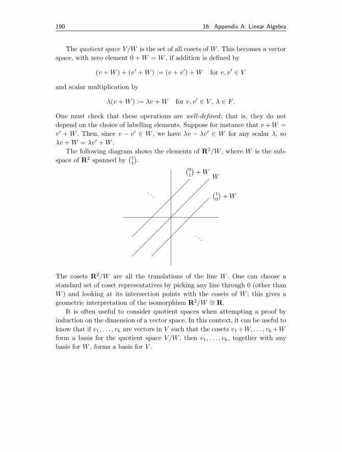
190 16. Appendix A: Linear Algebra

The quotient space V/W is the set of all cosets of W . This becomes a vectorspace, with zero element 0 + W = W , if addition is defined by

(v + W ) + (v′ + W ) := (v + v′) + W for v, v′ ∈ V

and scalar multiplication by

λ(v + W ) := λv + W for v, v′ ∈ V , λ ∈ F .

One must check that these operations are well-defined ; that is, they do notdepend on the choice of labelling elements. Suppose for instance that v + W =v′ + W . Then, since v − v′ ∈ W , we have λv − λv′ ∈ W for any scalar λ, soλv + W = λv′ + W .

The following diagram shows the elements of R2/W , where W is the sub-space of R2 spanned by

(11

).

W

(10

)+ W

(01

)+ W

. . .

. . .

The cosets R2/W are all the translations of the line W . One can choose astandard set of coset representatives by picking any line through 0 (other thanW ) and looking at its intersection points with the cosets of W ; this gives ageometric interpretation of the isomorphism R2/W ∼= R.

It is often useful to consider quotient spaces when attempting a proof byinduction on the dimension of a vector space. In this context, it can be useful toknow that if v1, . . . , vk are vectors in V such that the cosets v1 +W, . . . , vk +W

form a basis for the quotient space V/W , then v1, . . . , vk, together with anybasis for W , forms a basis for V .

16.2 Linear Maps 191

16.2 Linear Maps

Let V and W be vector spaces over a field F . A linear map (or linear transfor-mation) x : V → W is a map satisfying

x(λu + μv) = λx(u) + μx(v) for all u, v ∈ V and λ, μ ∈ F .

A bijective linear map between two vector spaces is an isomorphism. We assumethe reader knows about the definitions of the image and kernel of a linear map,and can prove the rank-nullity theorem,

dimV = dim imx + dimkerx.

A corollary of the rank-nullity theorem is that if dimV = dimW andx : V → W is injective, then, since dim imx = dimV , x is an isomorphism.One can draw the same conclusion if instead we know that x is surjective. Werefer to this type of reasoning as an argument by dimension counting.

We can now state the isomorphism theorems for vector spaces.

Theorem 16.1 (Isomorphism theorems for vector spaces)

(a) If x : V → W is a linear map, then kerx is a subspace of V , imx is asubspace of W , and

V/ ker x ∼= im x.

(b) If U and W are subspaces of a vector space, (U + W )/W ∼= U/(U ∩ W ).

(c) Suppose that U and W are subspaces of a vector space V such that U ⊆ W .Then W/U is a subspace of V/U and (V/U)/(W/U) ∼= V/W .

Proof

For part (a), define a map ϕ : V/ ker x → im x by

ϕ(v + kerx) = x(v).

This map is well-defined since if v + ker x = v′ + ker x then v − v′ ∈ ker x, soϕ(v + ker x) = x(v) = x(v′) = ϕ(v′ + ker x). It is routine to check that ϕ islinear, injective, and surjective, so it gives the required isomorphism.

To prove (b), consider the composite of the inclusion map U → U + W

with the quotient map U + W → (U + W )/W . This gives us a linear mapU → (U + W )/W . Under this map, x ∈ U is sent to 0 ∈ (U + W )/W if andonly if x ∈ W , so its kernel is U ∩ W . Now apply part (a).

Part (c) can be proved similarly; we leave this to the reader.


Parts (a), (b) and (c) of this theorem are known respectively as the first,second, and third isomorphism theorems. See Exercise 16.5 for one application.

16.3 Matrices and Diagonalisation

Suppose that x : V → V is a linear transformation of a finite-dimensionalvector space V . Let {v1, . . . , vn} be a basis of V . Using this basis, we maydefine scalars aij by

x(vj) =n∑

i=1

aijvi.

We say that the n×n matrix A with entries (aij) is the matrix of x with respectto our chosen basis. Conversely, given a basis of V and a matrix A, we can usethe previous equation to define a linear map x, whose matrix with respect tothis basis is A.

Exercise 16.1

(i) Let x : V → V and y : V → V be linear maps with matrices A and B

with respect to a basis of V . Show that, with respect to this basis,the matrix of the composite map yx is the matrix product BA.

(ii) Suppose that x has matrix A with respect to the basis v1, . . . , vn

of V . Let w1, . . . , wn be another basis of V . Show that the matrixof A in this new basis is P−1AP where the matrix P = (pij) isdefined by

wj =n∑

i=1

pijvi.

Matrices related in this way are said to be similar.

It had been said that “a true gentleman never takes bases unless he reallyhas to.” We generally agree with this sentiment, preferring to use matricesonly when they are necessary for explicit computations (for example in Chap-ter 12 when we look at the classical Lie algebras). When we are obliged toconsider matrices, then we can at least try to choose bases so that they are ofa convenient form.

Recall that a non-zero vector v ∈ V such that x(v) = λv is said to be aneigenvector of x with corresponding eigenvalue λ. The eigenspace for eigen-value λ is the vector subspace

{v ∈ V : x(v) = λv}.

16.3 Matrices and Diagonalisation 193

It is an elementary fact that non-zero vectors in different eigenspaces arelinearly independent. (This will often be useful for us; for example, see step 1in the proof of Theorem 8.5.)

The linear map x can be represented by a diagonal matrix if and only if V

has a basis consisting of eigenvectors for x. This is the same as saying that thespace V is a direct sum of x-eigenspaces,

V = Vλ1 ⊕ Vλ2 ⊕ . . . ⊕ Vλr ,

where the λi are the distinct eigenvalues of x. If this is the case, we say that x

is diagonalisable.Note that λ ∈ C is an eigenvalue of x if and only if ker(x − λ1V ) is non-

zero, which is the case if and only if det(x − λ1V ) = 0. The eigenvalues of x

are therefore the roots of the characteristic polynomial of x, defined by

cx(X) = det(x − X1V ),

where X is an indeterminant. Since over C any non-constant polynomial has aroot, this shows that any linear transformation of a complex vector space hasan eigenvalue.

The characteristic polynomial of x does not in itself give enough informationto determine whether x is diagonalisable — consider for example the matrices(

1 00 1

),

(1 10 1

).

To get further, one needs the minimal polynomial. The minimal polynomialof x is the monic polynomial of least degree which kills x, so m(X) = Xd +ad−1X

d−1 + . . . + a1X + a0 is the minimal polynomial of x if

xd + ad−1xd−1 + . . . + a1x + a01V = 0

and the degree d is as small as possible.An important property of the minimal polynomial is that if f(X) is any

polynomial such that f(x) = 0 then m(X) divides f(X).

Exercise 16.2

Prove this assertion by using polynomial division to write f(X) =a(X)m(X) + r(X), where the remainder polynomial r(X) is either 0or has degree less than that of m(X), and then showing that r(x) = 0.

By the famous theorem of Cayley–Hamilton (see Exercise 16.4), the minimalpolynomial of x divides the characteristic polynomial of x. We now explore someof the arguments in which the minimal polynomial is used.


16.3.1 The Primary Decomposition Theorem

Theorem 16.2 (Primary decomposition theorem)

Suppose the minimal polynomial of x factorises as

(X − λ1)a1 . . . (X − λr)ar ,

where the λi are distinct and each ai ≥ 1. Then V decomposes as a direct sumof x-invariant subspaces Vi,

V = V1 ⊕ V2 ⊕ . . . ⊕ Vr,

where Vi = ker(x − λi1V )ai . The subspaces Vi are said to be the generalisedeigenspaces of x.

This theorem may be proved by repeatedly applying the following lemma.

Lemma 16.3

If f(X) ∈ C[X] and g(X) ∈ C[X] are coprime polynomials such thatf(x)g(x) = 0, then im f(x) and im g(x) are x-invariant subspaces of V . More-over,

(i) V = im f(x) ⊕ im g(x), and

(ii) im f(x) = ker g(x) and im g(x) = ker f(x).

Proof

If v = f(x)w, then xv = f(x)xw, so the subspaces im f(x) and im g(x) arex-invariant. By Euclid’s algorithm, there exist polynomials a(X), b(X) ∈ C[X]such that a(X)f(X) + b(X)g(X) = 1, so for any v ∈ V ,

f(x)(a(x)v) + g(x)(b(x)v) = v. (�)

This shows that V = im f(x) + im g(x). If v ∈ im g(x) with, say, v = g(x)w,then f(x)v = f(x)g(x)w = 0, so im g(x) ⊆ ker f(x). On the other hand, iff(x)v = 0, then by (�), v = g(x)(b(x)v) so v ∈ im g(x). Finally, if

v ∈ im f(x) ∩ im g(x) = ker f(x) ∩ ker g(x),

then as f(x)a(x)v = a(x)f(x)v = 0 and similarly b(x)g(x) = 0, it followsfrom (�) that v = 0.

The following criterion for a linear map to be diagonalisable follows directlyfrom the primary decomposition theorem.

16.3 Matrices and Diagonalisation 195

Theorem 16.4

Let x : V → V be a linear map of a vector space V . Then x is diagonalisableif and only if the minimal polynomial of x splits as a product of distinct linearfactors.

Corollary 16.5

Let x : V → V be a diagonalisable linear transformation. Suppose that U is asubspace of V which is invariant under x, that is, x(u) ∈ U for all u ∈ U .

(a) The restriction of x to U is diagonalisable.

(b) Given any basis of U consisting of eigenvectors for x, we may extend thisbasis to a basis of V consisting of eigenvectors for x.

Proof

Let m(X) be the minimal polynomial of x : V → V . Let mU (X) be theminimal polynomial of x, regarded just as a linear transformation of U . Thenm(x)(U) = 0, so mU (X) must divide m(X). Hence mU (X) is a product ofdistinct linear factors.

Now let V = Vλ1 ⊕ . . . ⊕ Vλr be the decomposition of V into distincteigenspaces of x. Since x acts diagonalisably on U we have

U = U ∩ Vλ1 ⊕ . . . ⊕ U ∩ Vλr .

Extend the basis of each U ∩ Vλito a basis of Vλi

. This gives us a basis of V

of the required form.

We now give another application of the primary decomposition theorem.

Lemma 16.6

Suppose that x has minimal polynomial

f(X) = (X − λ1)a1 . . . (X − λr)ar ,

where the λi are pairwise distinct. Let the corresponding primary decomposi-tion of V as a direct sum of generalised eigenspaces be

V = V1 ⊕ . . . ⊕ Vr,

where Vi = ker(x − λi1V )ai . Then, given any μ1, . . . , μr ∈ C, there is a poly-nomial p(X) such that

p(x) = μ11V1 + μ21V2 . . . + μr1Vr.


Proof

Suppose we could find a polynomial f(X) ∈ C[X] such that

f(X) ≡ μi mod (X − λi)ai .

Take v ∈ Vi = ker(x−λi1V )ai . By our supposition, f(X) = μi+a(X)(X−λi)ai

for some polynomial a(X). Hence

f(x)v = μi1Viv + a(x)(x − λi)aiv = μiv,

as required.The polynomials (X − λ1)a1 . . . , (X − λr)ar are coprime. We may therefore

apply the Chinese Remainder Theorem, which states that in these circum-stances the map

C[X] →r⊕

i=1

C[X](X − λi)ai

f(X) �→ (f(X) mod (X − λ1)a1 , . . . , f(X) mod (X − λr)ar )

is surjective, to obtain a suitable p(X).

In terms of matrices, this lemma says that

p(x) =

⎛⎜⎜⎜⎝

μ1In1 0 . . . 00 μ2In2 . . . 0...

.... . .

...0 0 . . . μrInr

⎞⎟⎟⎟⎠ ,

where ni = dimVi and Is denotes the s × s identity matrix.

16.3.2 Simultaneous Diagonalisation

In the main text, we shall several times have a finite family of linear transfor-mations of a vector space V , each of which is individually diagonalisable. Whencan one find a basis of V in which they are all simultaneously diagonal?

Lemma 16.7

Let x1, . . . , xk : V → V be diagonalisable linear transformations. There is abasis of V consisting of simultaneous eigenvectors for all the xi if and only ifthey commute. (That is, xixj = xjxi for all pairs i, j.)

16.4 Interlude: The Diagonal Fallacy 197

Proof

For the “only if” direction we note that diagonal matrices commute with oneanother, so if we can represent all the xi by diagonal matrices, they mustcommute.

The main step in the “if” direction is the case k = 2. Write V as a directsum of eigenspaces for x1, say V = Vλ1 ⊕ . . .⊕Vλr

, where the λi are the distincteigenvalues of x1. If v ∈ Vλi

then so is x2(v), for

x1x2(v) = x2x1(v) = x2(λiv) = λi(x2(v)).

We now apply Corollary 16.5(a) to deduce that x2 restricted to Vλi is di-agonalisable. A basis of Vλi

consisting of eigenvectors for x2 is automatically abasis of eigenvectors for x1, so if we take the union of a basis of eigenvectorsfor x2 on each Vλi

, we get a basis of V consisting of simultaneous eigenvectorsfor both x1 and x2.

The inductive step is left to the reader.

In Exercise 16.6, we give a small generalisation which will be needed in themain text.

16.4 Interlude: The Diagonal Fallacy

Consider the following (fallacious) argument. Let V be a 2-dimensional vectorspace, say with basis v1, v2. Let x : V → V be the linear map whose matrixwith respect to this basis is (

0 10 0

).

We claim that if U is a subspace of V such that x(U) ⊆ U , then either U = 0,U = Span{v1}, or U = V . Clearly each of these subspaces is invariant under x,so we only need to prove that there are no others. But since x(v2) = v1,Span{v2} is not x-invariant. (QED?)

Here we committed the diagonal fallacy : We assumed that an arbitrarysubspace of V would contain one of our chosen basis vectors. This assumptionis very tempting — which perhaps explains why it is so often made — but itis nonetheless totally unjustified.

Exercise 16.3

Give a correct proof of the previous result.


The following diagram (which is frequently useful as a counterexample inlinear algebra) illustrates how the fallacy we have been discussing gets its name.

Span{(11)}Span{(01)}

Span{(10)}

16.5 Jordan Canonical Form

Let V be a finite-dimensional complex vector space and let x : V → V be alinear map. Exercise 6.2 outlines the proof that one can always find a basis of V

in which x is represented by an upper triangular matrix. For many purposes,this result is sufficient. For example, it implies that a nilpotent map may berepresented by a strictly upper triangular matrix, and so nilpotent maps havetrace 0.

Sometimes, however, one needs the full strength of Jordan canonical form.A general matrix in Jordan canonical form looks like⎛

⎜⎜⎜⎝A1 0 . . . 00 A2 . . . 0...

.... . .

...0 0 . . . Ar

⎞⎟⎟⎟⎠ ,

where each Ai is a Jordan block matrix Jt(λ) for some t ∈ N and λ ∈ C:

Jt(λ) =

⎛⎜⎜⎜⎜⎜⎜⎜⎜⎝

λ 1 0 . . . 0 00 λ 1 . . . 0 00 0 λ . . . 0 0...

......

. . ....

...0 0 0 . . . λ 10 0 0 . . . 0 λ

⎞⎟⎟⎟⎟⎟⎟⎟⎟⎠

t×t

.

We now outline a proof that any linear transformation of a complex vectorspace can be represented by a matrix in Jordan canonical form.

16.5 Jordan Canonical Form 199

The first step is to reduce to the case where xq = 0 for some q ≥ 1; thatis, x is a nilpotent linear map.

By the primary decomposition theorem, it suffices to consider the casewhere x has only one eigenvalue, say λ. Then by considering x − λ1V , wemay reduce to the case where x acts nilpotently. So it suffices to show that anilpotent transformation can be put into Jordan canonical form.

16.5.1 Jordan Canonical Form for Nilpotent Maps

We shall work by induction on dimV .Suppose that xq = 0 and xq−1 �= 0. Let v ∈ V be any vector such that

xq−1v �= 0. One can check that the vectors v, xv, . . . , xq−1v are linearly inde-pendent. Their span, U say, is an x-invariant subspace of V . With respect tothe given basis of U , the matrix of x : U → U is the q × q matrix

Jq(0) =

⎛⎜⎜⎜⎜⎜⎝

0 1 0 . . . 00 0 1 . . . 0...

......

. . ....

0 0 0 . . . 10 0 0 . . . 0

⎞⎟⎟⎟⎟⎟⎠ .

Suppose we can find an x-invariant complementary subspace to U ; that is,a subspace C such that x maps C into C and V = U ⊕ C. Then, by induction,there is a basis of C in which the matrix of x restricted to C is in Jordancanonical form. Putting the bases of C and U together gives us a suitable basisfor V .

To show that a suitable complement exists, we use a further induction on q.If q = 1, then x = 0 and any vector space complement to Span {v} will do.Now suppose we can find complements when xq−1 = 0.

Consider imx ⊆ V . On imx, x acts as a nilpotent linear map whose q − 1power is 0, so by induction on q we get

im x = Span{xv, . . . , xq−1v

}⊕ W

for some x-invariant subspace W . Note that U∩W = 0. Our task is to extend W

to a suitable x-invariant complement for U in V .Suppose first that W = 0. In this case, im x = Span

{xv, . . . , xq−1v

}and

ker x ∩ im x =⟨xq−1v

⟩. Extend xq−1v to a basis of kerx, say by v1, . . . , vs. By

the rank-nullity formula

v, xv . . . , xq−1v, v1, . . . , vs


is a basis of V . The subspace spanned by v1, . . . , vs is an x-invariant complementto U .

Now suppose that W �= 0. Then x induces a linear transformation, say x,on V/W . Let v = v + W . Since im x = Span

{xv, . . . , xq−1v

}, the first case im-

plies that there is an x-invariant complement in V/W to Span{v, xv, . . . xq−1v

}.

The preimage of this complement in V is a suitable complement to U .

16.6 Jordan Decomposition

Any linear transformation x of a complex vector space V has a Jordan de-composition, x = d + n, where d is diagonalisable, n is nilpotent, and d and n

commute.One can see this by putting x into Jordan canonical form: Fix a basis of V

in which x is represented by a matrix in Jordan canonical form. Let d be themap whose matrix in this basis has the diagonal entries of x down its diagonal,and let n = x − d. For example we might have

x =

⎛⎝1 1 0

0 1 00 0 1

⎞⎠ , d =

⎛⎝1 0 0

0 1 00 0 1

⎞⎠ , n =

⎛⎝0 1 0

0 0 00 0 0

⎞⎠ .

As n is represented by a strictly upper triangular matrix, it is nilpotent. Weleave it to the reader to check that d and n commute.

In applications it is useful to know that d and n can be expressed as poly-nomials in x. In the following lemma, we also prove a related result that isneeded in Chapter 9.

Lemma 16.8

Let x have Jordan decomposition x = d+n as above, where d is diagonalisable,n is nilpotent, and d, n commute.

(a) There is a polynomial p(X) ∈ C[X] such that p(x) = d.

(b) Fix a basis of V in which d is diagonal. Let d be the linear map whosematrix with respect to this basis is the complex conjugate of the matrixof d. There is a polynomial q(X) ∈ C[X] such that q(x) = d.

16.7 Bilinear Algebra 201

Proof

Let λ1, . . . , λr be the distinct eigenvalues of x. The minimal polynomial of x isthen

m(X) = (X − λ1)a1 . . . (X − λr)ar ,

where ai is the size of the largest Jordan block with eigenvalue λi.We can now apply Lemma 16.6 to get the polynomials we seek. For part

(a) take μi = λi, and for part (b) take μi = λi.

Part (a) of this lemma can be used to prove that the Jordan decompositionof a linear map is unique — see Exercise 16.7 below.

16.7 Bilinear Algebra

As well as the books already mentioned, we recommend Artin’s GeometricAlgebra [1] for further reading on bilinear algebra. From now on, we let V bean n-dimensional vector space over a field F .

16.7.1 Dual spaces

The dual space of V , denoted V �, is by definition the set of all linear maps fromV to F . Thus, if f, g ∈ V �, then f + g is defined by (f + g)(v) = f(v) + g(v)for v ∈ V , and if λ ∈ F , then λf is defined by (λf)(v) = λf(v).

Given a vector space basis {v1, . . . , vn} of V , one defines the associateddual basis of V as follows. Let fi : V → F be the linear map defined on basiselements by

fi(vj) =

{1 i = j

0 i �= j.

It is not hard to check that f1, . . . , fn is a basis for V �. In particular dimV =dimV �.

The dual space of V ∗ can be identified with V in a natural way. Givenv ∈ V , we may define an evaluation map εv : V ∗ → F by

εv(f) := f(v) for all f ∈ V ∗.

It is straightforward to check that εv is linear and so belongs to the dual spaceof V �; that is, to V ��. Moreover, the map v �→ εv (which we might call ε)from V to V �� is itself linear. We claim that ε : V → V �� is an isomorphism.


Since we have already shown that dimV = dimV � = dimV ��, it is sufficientto show that εv = 0 implies v = 0. One way to do this is as follows. If v �= 0,then we may extend v to a basis of V and take the associated dual basis.Then f1(v) = 1 and hence εv(f1) �= 0, so εv �= 0.

If U is a subspace of V we let

U◦ = {f ∈ V � : f(u) = 0 for all u ∈ U}be the annihilator of U in V �. One can show that U◦ is a subspace of V � andthat

dimU + dimU◦ = dimV.

A proof of the last statement is outlined in Exercise 16.8.Given a subspace W of V ∗, we can similarly define the annihilator of W

in V ��. Under the identification of V �� with V , the annihilator of W becomes

W 0 = {v ∈ V : f(v) = 0 for all f ∈ W}.

In particular, we have dimW + dimW 0 = dimV .

16.7.2 Bilinear Forms

Definition 16.9

A bilinear form on V is a map

(−,−) : V × V → F

such that

(λ1v1 + λ2v2, w) = λ1(v1, w) + λ2(v2, w),

(v, μ1w1 + μ2w2) = μ1(v, w1) + μ2(v, w2),

for all v, w, vi, wi ∈ V and λi, μi ∈ F .

For example, if F = R and V = Rn, then the usual dot product is a bilinearform on V .

As for linear transformations, we can represent bilinear forms by matrices.Suppose that (−,−) is a bilinear form on the vector space V and that V hasbasis {v1, . . . , vn}. The matrix of (−,−) with respect to this basis is A = (aij),where aij = (vi, vj). If we change the basis, say to {w1, . . . , wn}, then the newmatrix representing (−,−) is P tAP where P = (pij) is the n×n matrix definedby

wj =n∑

i=1

pijvi.


Matrices related in this way are said to be congruent.Conversely, given an n × n matrix S = (sij), we may define a bilinear form

on V by setting(vi, vj) = sij

and extending “bilinearly” to arbitrary elements in V × V . That is, if v =∑i λivi and w =

∑j μjvj with λi and μj scalars, then

(v, w) =n∑

i=1

n∑j=1

sijλiμj .

The last equation may be written in matrix form as

(v, w) = (λ1 . . . λn)

⎛⎜⎝

s11 . . . s1n

.... . .

...sn1 . . . snn

⎞⎟⎠⎛⎜⎝

μ1...

μn

⎞⎟⎠ .

Given a subset U of V , we set

U⊥ := {v ∈ V : (u, v) = 0 for all u ∈ U}.

This is always a subspace of V . We say that the form (−,−) is non-degenerateif V ⊥ = {0}.

Example 16.10

Let U be a 2m-dimensional vector space with basis u1, . . . , u2m, and let

S =(

0 Im

Im 0

),

where Im is the identity matrix of size m × m. The bilinear form associatedto S may be shown to be non-degenerate. (For example, this follows fromExercise 16.9.) However, the restriction of the form to the subspace spannedby u1, . . . , um is identically zero.

For a more substantial example, see Exercise 16.10 below.

We now explain the connection between bilinear forms and dual spaces.Let ϕ : V → V � be the linear map defined by ϕ(v) = (−, v). That is, ϕ(v)is the linear map sending u ∈ V to (u, v). If (−,−) is non-degenerate, thenker ϕ = 0, so by dimension counting, ϕ is an isomorphism. Thus every elementof V � is of the form (−, v) for a unique v ∈ V ; this is a special case of the Rieszrepresentation theorem. A small generalisation of this argument can be used toprove the following lemma — see Exercise 16.8.


Lemma 16.11

Suppose that (−,−) is a non-degenerate bilinear form on the vector space V .Then, for all subspaces U of V , we have

dimU + dimU⊥ = dimV.

If U ∩ U⊥ = 0, then V = U ⊕ U⊥ and, furthermore, the restrictions of (−,−)to U and to U⊥ are non-degenerate.

16.7.3 Canonical Forms for Bilinear Forms

Definition 16.12

Suppose that (−,−) : V × V → F is a bilinear form. We say that (−,−) issymmetric if (v, w) = (w, v) for all v, w ∈ V and that (−,−) is skew-symmetricor symplectic if (v, w) = −(w, v) for all v, w ∈ V .

In the main text, we shall only need to deal with bilinear forms that areeither symmetric or skew-symmetric. For such a form, (v, w) = 0 if and onlyif (w, v) = 0. When F = R, a symmetric bilinear form with (v, v) ≥ 0 for allv ∈ V and such that (v, v) = 0 if and only if v = 0 is said to be an innerproduct.

A vector v ∈ V is said to be isotropic with respect to a form (−,−) if(v, v) = 0. For example, if (−,−) is symplectic and the characteristic of thefield is not 2, then all elements in V are isotropic. But symmetric bilinearforms can also have isotropic vectors (as long as they do not come from innerproducts). For example, in Example 16.10 above, the basis of U consists ofisotropic vectors.

If (−,−) is non-degenerate and v ∈ V is isotropic, then there exists somew ∈ V such that (v, w) �= 0. Clearly v and w must be linearly independent.This observation motivates the following lemma (which we use in Appendix C).

Lemma 16.13

Suppose V has a non-degenerate bilinear form (−,−). Suppose U1 and U2 aretrivially-intersecting subspaces of V such that (u, v) = 0 for all u, v ∈ U1 andfor all u, v ∈ U2 and that (−,−) restricted to U1 ⊕U2 is non-degenerate. Then,if {u1, . . . , um} is a basis of U1 there is a basis {u′

1, . . . , u′n}, of U2 such that

(ui, u′j) =

{1 i = j

0 i �= j.


Proof

Consider the map γ : U2 → U∗1 defined by γ(v) = (−, v). That is, γ(v)(u) =

(u, v) for all u ∈ U1. This map is linear, and it is injective because the restrictionof (−,−) to U1 ⊕ U2 is non-degenerate, so we have

dimU2 ≤ dimU∗1 = dimU1.

By symmetry, we also have dim U1 ≤ dimU2, so γ must be an isomorphism.Given the basis {u1, . . . , un} of U1, let {f1, . . . , fn} be the corresponding

dual basis of U∗1 . For 1 ≤ j ≤ n, let u′

j ∈ U2 be the unique vector such thatγ(u′

j) = fj . Then we have

(ui, u′j) = fj(ui) =

{1 i = j

0 i �= j

as required.

Note that if (−,−) is symmetric, then the matrix of (−,−) with respect tothis basis of U1 ⊕ U2 is (

0 Im

Im 0

).

An analogous result holds if (−,−) is skew-symmetric.In the following we assume that the characteristic of F is not 2.

Lemma 16.14

Let (−,−) be a non-degenerate symmetric bilinear form on V . Then there is abasis {v1, . . . , vn} of V such that (vi, vj) = 0 if i �= j and (vi, vi) �= 0.

Proof

We use induction on n = dimV . If n = 1, then the result is obvious, so we mayassume that dim V ≥ 2.

Suppose that (v, v) = 0 for all v ∈ V . Then, thanks to the identity

(v + w, v + w) = (v, v) + (w, w) + 2(v, w),

we have (v, w) = 0 for all v, w ∈ V , which contradicts our assumption that(−,−) is non-degenerate. (This is where we need our assumption on the char-acteristic of F .)

We may therefore choose v ∈ V so that (v, v) �= 0. Let U = Span{v}. Byhypothesis U ∩U⊥ = {0}, so by Lemma 16.11 we have V = U ⊕U⊥. Moreover,


the restriction of (−,−) to U⊥ is non-degenerate. By the inductive hypothesis,there is a basis of U⊥, say {v2, . . . , vn}, such that (vi, vj) = 0 for i �= j and(vi, vi) �= 0 for 2 ≤ i ≤ n. Since also (v, vj) = 0 for j �= 1, if we put v1 = v thenthe basis {v1, . . . , vn} has the required properties.

Depending on the field, we may be able to be more precise about the diag-onal entries di = (vi, vi). Suppose that F = R. Then we may find λi ∈ R suchthat λ2

i = |di|. By replacing vi with vi/λi, we may assume that (vi, vi) = ±1.The bilinear form (−,−) is an inner product if and only if (vi, vi) > 0 for all i.

If F = C, then we can find λi so that λ2i = di, and hence we may assume

that (vi, vi) = 1 for all i, so the matrix representing (−,−) is the n×n identitymatrix.

Lemma 16.15

Suppose that (−,−) is a non-degenerate symplectic bilinear form on V . Thenwe have dimV = 2m for some m. Moreover, there is a basis of V such that(vi, vi+n) �= 0 for 1 ≤ i ≤ n and (vi, vj) = 0 if |i − j| �= n.

Proof

Again we work by induction dimV . Let 0 �= v ∈ V . Since (−,−) is non-degenerate, we may find w ∈ V such that (v, w) �= 0. Since v, w are isotropic,it is clear that {v, w} is linearly independent. Set v1 = v and v2 = w. IfdimV = 2, then we are done. Otherwise, let U be the orthogonal complementof the space W spanned by v1, v2. One shows easily that U ∩ W = {0} andthat by dimension counting V = U ⊕ W . Now, the restriction of (−,−) to U isnon-degenerate and also symplectic. The result now follows by induction.

When F = R or F = C, it is again useful to scale the basis elements. Inparticular, when F = C we may arrange that the matrix representing (−,−)has the form (

0 Im

−Im 0

),

where Im is the m × m identity matrix.

EXERCISES

16.4. Let x : V → V be a linear transformation of a complex vector space.By the result mentioned at the start of §16.5, we may find a basis

Exercises 207

v1, . . . , vn of V in which x is represented by an upper triangularmatrix. Let λ1, . . . , λn be the diagonal entries of this matrix. Showthat if 1 ≤ k ≤ n then

(x − λk1V ) . . . (x − λn1V )V ⊆ Span{v1, . . . , vk−1}.

Hence prove the Cayley–Hamilton theorem for linear maps on com-plex vector spaces.

16.5. Let A be an m × n matrix with entries in a field F . Show that thereis a bijective correspondence between solution sets of the equationAx = y for y ∈ im A and elements of the quotient vector spaceFn/ ker A.

16.6.† Let V be a finite-dimensional vector space.

(i) Show that Hom(V, V ), the set of linear transformations of V , isa vector space, and determine its dimension.

(ii) Let A ⊆ Hom(V, V ) be a collection of commuting linear maps,each individually diagonalisable. Show that there is a basis of V

in which all the elements of A are simultaneously diagonal.

(iii)� Can the assumption that V is finite-dimensional be dropped?

16.7.† Suppose that x : V → V is a linear map on a vector space V andthat x = d + n = d′ + n′ where d, d′ are diagonalisable and n, n′ arenilpotent, d and n commute and d′ and n′ commute. Show that d

and d′ commute. Hence show that d − d′ = n′ − n = 0. Deduce thatthe Jordan decomposition of a linear map is unique.

16.8. Let U be a subspace of the F -vector space V .

(i) Consider the restriction map r : V � → U�, which takes a linearmap f : V → F and regards it just as a map on U . Show thatker r = U◦ and im r = U�. Hence prove that

dimU + dimU0 = dimV.

(ii) Now suppose that (−,−) is a non-degenerate bilinear form onV . By considering the linear map ϕ : V → U� defined by

ϕ(v)(u) = (u, v),

show that dimU + dimU⊥ = dimV .


16.9. Let V be a finite-dimensional vector space with basis {v1, . . . , vn}.Suppose that (−,−) is a bilinear form on V , and let aij = (vi, vj).Show that V ⊥ = {0} if and only if the matrix A = (aij) is non-singular.

16.10. Let V be a finite-dimensional vector space and let Hom(V, V ) be thevector space of all linear transformations of V . Show that

(x, y) �→ tr(xy)

defines a non-degenerate symmetric bilinear form on Hom(V, V ). ByExercise 16.8(ii) this form induces an isomorphism

Hom(V, V ) → Hom(V, V )�.

What is the image of the identity map 1V : V → V under thisisomorphism?

17Appendix B: Weyl’s Theorem

We want to show that any finite-dimensional representation of a complexsemisimple Lie algebra is a direct sum of irreducible representations. This isknown as Weyl’s Theorem; it is a fundamental result in the representationtheory of Lie algebras. We used it several times in Chapter 9 to decompose arepresentation of sl(2,C) into a direct sum of irreducible representations.

As usual, all Lie algebras and representations in this chapter are finite-dimensional.

17.1 Trace Forms

When we proved that a complex semisimple Lie algebra is a direct sum of simpleLie algebras (or, equivalently, that the adjoint representation is completelyreducible), we used the Killing form κ. Now we use a generalisation of theKilling form known as the trace form.

Let L be a Lie algebra and let V be an L-module. Write ϕ : L → gl(V ) forthe corresponding representation. Define the trace form βV : L × L → C by

βV (x, y) := tr(ϕ(x) ◦ ϕ(y)) for x, y ∈ L.

This is a symmetric bilinear form on L. In the special case where V = L and ϕ

is the adjoint representation, it is just the Killing form. The trace form βV isassociative; that is,

βV ([x, y], z) = βV (x, [y, z]) for all x, y, z ∈ L,

210 17. Appendix B: Weyl’s Theorem

as an easy calculation will show. This implies, as it did for the Killing form,that if we define the radical of β by

radβV := {x ∈ L : βV (x, y) = 0 for all y ∈ L},

then radβV is an ideal of L.So far, our definitions make sense for any representation of an arbitrary Lie

algebra. For semisimple Lie algebras, we have the following lemma.

Lemma 17.1

Suppose L is a complex semisimple Lie algebra and ϕ : L → gl(V ) is a faithfulrepresentation (that is, ϕ is injective). Then radβV is zero and so βV is non-degenerate.

Proof

Let I = radβV . For any x, y ∈ I, we have βV (x, y) = 0. Now apply Proposi-tion 9.3 to the Lie subalgebra ϕ(I) of gl(V ). This gives that ϕ(I) is solvableand hence, since ϕ is injective, that I is solvable. But L is semisimple, so it hasno non-zero solvable ideals, and therefore I is zero.

With the assumptions of the previous lemma, we may use the bilinearform βV to identify L with L�: namely, given θ ∈ L�, there is a unique el-ement y ∈ L such that β(x, y) = θ(x) for all x ∈ L. Let x1, . . . , xn be a vectorspace basis of L and let θ1, . . . , θn be the dual basis of L�. We use this identifi-cation to find elements y1, . . . , yn such that βV (x, yj) = θj(x) for all x ∈ L, orequivalently such that

βV (xi, yj) =

{1 i = j

0 i �= j.

Lemma 17.2

Suppose that x ∈ L and [xi, x] =∑

j aijxj . Then, for each t with 1 ≤ t ≤ n,we have

[x, yt] =n∑

i=1

atiyi.

17.2 The Casimir Operator 211

Proof

We have

βV ([xi, x], yt) =n∑

j=1

aijβV (xj , yt) = ait.

We write [x, yt] =∑n

s=1 btsys. By associativity,

ait = βV ([xi, x], yt) = βV (xi, [x, yt]) =n∑

s=1

btsβV (xi, ys) = bti.

17.2 The Casimir Operator

Let L be a complex semisimple Lie algebra and let V be a faithful L-modulewith associated representation ϕ : L → gl(V ). We continue using the trace formβV and the two bases of L defined above. The Casimir operator associated toϕ is the linear map c : V → V defined by

c(v) =n∑

i=1

xi · (yi · v)

in terms of the module action. In the language of representations, c becomes

c =n∑

i=1

ϕ(xi)ϕ(yi).

Lemma 17.3

(a) The map c : V → V is an L-module homomorphism.

(b) We have tr(c) = dimL.

Proof

For (a), we must show that c(x · v) − x · (c(v)) = 0 for all v ∈ V and x ∈ L, soconsider

c(x · v) − x · (cv) =n∑

i=1

xi(yi(xv)) −n∑

i=1

x(xi(yiv)).

Add the equation −xi(x(yiv)) + xi(x(yiv)) = 0 to each term in the sum to get

c(x · v) − x · (cv) =n∑

i=1

xi([yi, x]v) +n∑

i=1

[xi, x](yiv).


If [xi, x] =∑n

j=1 aijxj , then by the previous lemma we know that [yi, x] =∑nj=1 ajiyj . Substituting this into the previous equation gives

c(x · v) − x · (cv) =∑i,j

−ajixi(yjv) +∑i,j

aijxj(yiv) = 0.

For (b), note that

tr c =n∑

i=1

tr(ϕ(xi) ◦ ϕ(yi)) =n∑

i=1

βV (xi, yi) = n

and n = dimL.

Theorem 17.4 (Weyl’s Theorem)

Let L be a complex semisimple Lie algebra. Every finite-dimensional L-moduleis completely reducible.

Proof

Let V be such an L-module, and let ϕ : L → gl(V ) be the correspondingrepresentation. Suppose that W is a submodule of V . By induction on dimV

it is enough to show that W has a complement in V , that is, there is someL-submodule C of V such that V = W ⊕ C.

We may assume that ϕ is one-to-one, for if not then we can replace L by theLie algebra L/I, where I is the kernel of ϕ. By Lemma 9.12, L/I is semisimple,and if we view V as a module for L/I, then the corresponding representation isone-to-one. It is clear that the submodule structure of V as a module for L/I

is the same as the submodule structure of V as a module for L.We first prove Weyl’s Theorem in the special case where dim W = dimV −1.

In this case, the factor module V/W is the trivial L-module since the derivedalgebra L′ acts trivially on any one-dimensional L-module, and for L semisimplewe have L′ = L (see Exercise 9.9). Hence

x ∈ L, v ∈ V =⇒ x · v ∈ W. (�)

We now proceed by induction on dimW .

Step 1: Assume for a start that W is simple. Let c : V → V be the Casimiroperator of V . Since c is an L-module homomorphism, its kernel is a submoduleof V . Our aim is to show that ker c is a suitable complement for W .

As we have noted in (�), for x ∈ L and v ∈ V we have x · v ∈ W . Thisimplies that c(v) ∈ W for all v ∈ V . In particular, this shows that c is not ontoand therefore ker c �= 0 by the rank-nullity formula.

17.2 The Casimir Operator 213

The restriction of c to W is also an L-module homomorphism, so by Schur’sLemma there is some λ ∈ C such that c(w) = λw for all w ∈ W . We claimthat λ �= 0. To see this, we calculate the trace of c in two ways. First, usingc(V ) ⊆ W and c(w) = λw for w ∈ W , we get that the trace of c is equal toλ dimW . On the other hand, from Lemma 17.3 we know that the trace is equalto dimL, which is non-zero. Hence λ �= 0. We deduce that ker c ∩ W = 0. Itnow follows from dimension counting that W ⊕ ker c = V .

Step 2: For the inductive step, suppose that W1 is a proper submoduleof W . Then W/W1 is a submodule of V/W1, and the quotient is 1-dimensional,since by the third isomorphism theorem, we have

(V/W1)/(W/W1) ∼= V/W.

Moreover, dimV/W1 < dimV , so the inductive hypothesis applied to V/W1

gives thatV/W1 = W/W1 ⊕ X,

where X is a 1-dimensional L-submodule of V/W1. By the submodule corre-spondence, there is a submodule X of V containing W1 such that X = X/W1.

Now, dimX = 1 + dimW1, and dimX < dimV (otherwise we would haveW1 = W ), so we can also apply the inductive hypothesis to X and get X =W1 ⊕ C for some L-submodule C of X (and again dimC = 1). We claim thatV = W ⊕ C. By dimension counting, it is enough to show that W ∩ C = 0.The direct sum decomposition of V/W1 above implies that the image of W ∩X

under the quotient map V → V/W1 is zero. Hence W ∩ X ⊆ W1 and soW ∩ C ⊆ W1 ∩ C = 0.

This completes the proof of Weyl’s Theorem in the special case wheredimW + 1 = dimV .

We now consider the general case. Suppose W is an L-submodule of V .Consider the L-module M := Hom(V, W ) of linear maps from V to W . Recallfrom Exercise 7.12 that the action of L on M is defined by

(x · f)(v) = x · f(v) − f(x · v) for x ∈ L, f ∈ M, v ∈ V .

We can apply the result for the special case to M as follows. Let

MS := {f ∈ M : f↓W = λ1W for some λ ∈ C},

M0 := {f ∈ M : f↓W = 0},

where f↓W denotes the restricted map f : W → W . One can check that bothMS and M0 are L-submodules of M , and M0 ⊆ MS .

We claim that the quotient MS/M0 is 1-dimensional. Clearly, the identitymap 1V of V lies in MS but not in M0, so the coset of 1V is a non-zero element


in the quotient. Now if f ∈ MS satisfies f↓W = λ1W , then f − λ1V belongs toM0; that is, f + M0 = λ1V + M0.

We now apply Weyl’s Theorem for the special case. This tells us that MS =M0 ⊕ C for some L-submodule C of MS . Also, C is 1-dimensional and hencetrivial as an L-module, so C contains a non-zero element ϕ such that x · ϕ = 0for all x ∈ L. The condition x · ϕ = 0 just means that ϕ is an L-modulehomomorphism. By scaling ϕ we may assume that ϕ↓W = 1W .

Now we can get back to the original module V . Since ϕ is an L-modulehomomorphism, its kernel, say K, is a submodule of V . We claim that V =K ⊕ W . If v ∈ K ∩ W , then ϕ(v) = 0. On the other hand, the restriction ofϕ to W is the identity, so ϕ(v) = v. Therefore K ∩ W = 0. By the definitionof M , imϕ is contained in W . It now follows from the rank-nullity formula that

dimK = dimV − dim imϕ ≥ dimV − dimW,

so by dimension counting V = K + W . Hence V = K ⊕ W , as required.

EXERCISES

17.1. Let V be a representation of the complex semisimple Lie algebra L.Prove that the Casimir operator c : V → V is independent of thechoice of basis of L.

17.2. Show that the Casimir operator for the natural representation ofsl(2,C) with respect to the standard basis (h, e, f) of sl(2,C) is givenby

c(v) = (ef + fe + 12h

2)v.

Show that if V is any irreducible representation of sl(2,C), then theCasimir operator for V is given by a scalar multiple of this expres-sion.

17.3. Prove that a complex Lie algebra is semisimple if and only if all itsfinite-dimensional representations are completely reducible.

18Appendix C: Cartan Subalgebras

Suppose that L is a semisimple Lie algebra with Cartan subalgebra H and asso-ciated root system Φ. We want to show that if H1 is another Cartan subalgebraof L, with associated root system Φ1, then Φ1 is isomorphic to Φ. This showsfirst of all that the root system of a semisimple Lie algebra is well-defined (upto isomorphism) and secondly that semisimple Lie algebras with different rootsystems cannot be isomorphic.

The general proof of this statement is quite long and difficult and requiresseveral ideas which we have so far avoided introducing. So instead we give aproof that assumes that L is a classical Lie algebra. This will be sufficientto show that the only isomorphisms between the classical Lie algebras comefrom isomorphisms between their root systems; we used this fact at the endof Chapter 12. We then show how Serre’s Theorem and the classification ofChapter 14 can be used to give the result for a general semisimple Lie algebra.

We conclude by discussing the connection between our Cartan subal-gebras and the “maximal toral algebras” used by other authors, such asHumphreys [14].

18.1 Root Systems of Classical Lie Algebras

Let L be a classical Lie algebra, so L is defined as a particular subalgebra ofa matrix algebra gl(n,C). This gives us a practical way to show that the rootsystems corresponding to different Cartan subalgebras are isomorphic.

216 18. Appendix C: Cartan Subalgebras

Proposition 18.1

Let H and K be Cartan subalgebras of L. Suppose that there is an invertiblen×n matrix P such that PHP−1 ⊆ K and PLP−1 ⊆ L. Then the root systemscorresponding to H and K are isomorphic.

Proof

We first show that the hypotheses imply PHP−1 = K and PLP−1 = L.The latter follows just by dimension counting. For the former, we argue thatbecause an element of L is semisimple if and only if it is diagonalisable (seeTheorem 9.16) and, moreover, a conjugate of a diagonalisable matrix is diago-nalisable, the elements of P−1KP are semisimple. Hence P−1KP is an abeliansubalgebra of L consisting of semisimple elements and containing H. Since H

is a Cartan subalgebra, we must have H = P−1KP .Now let α be a root taken with respect to H, and let x ∈ L be in the

corresponding root space, so [h, x] = α(h)x for all h ∈ H. Then

[PhP−1, PxP−1] = P [h, x]P−1 = α(h)PxP−1.

Hence, if we define αP ∈ K� by

αP(k) = α(P−1kP ) for k ∈ K,

then PxP−1 is in the αP root space of K. Therefore α �→ αP is a one-to-onemap from the roots of H to the roots of K; by symmetry it is a bijection.

In fact, this map induces an isomorphism between the root systems corre-sponding to H and K. To check condition (b) in the definition of isomorphism(Definition 11.19), note that if α and β are roots with respect to H, then

〈αP , βP 〉 = αP(hβP

)= α(P−1hβP P ) = α(hβ) = 〈α, β〉 .

Here we used that hαP = PhαP−1; one way to prove this is to consider theaction of PhαP−1 on the K-root spaces where K acts as ±αP .

For the classical Lie algebras, we have a standard choice of Cartan sub-algebra, namely the subalgebra consisting of all diagonal matrices in the Liealgebra. So given a Cartan subalgebra H, we look for a basis of V = Cn inwhich the elements of H are diagonal. We can then apply Proposition 18.1with P as the change of basis matrix.

We start with the Lie algebras sl(n,C) for n ≥ 2. In this case, becausecommuting diagonalisable matrices may be simultaneously diagonalised, andconjugation preserves traces, the hypotheses for Proposition 18.1 are easilyseen to be satisfied.

18.2 Orthogonal and Symplectic Lie Algebras 217

18.2 Orthogonal and Symplectic Lie Algebras

We now consider sp(2m,C) for m ≥ 1 and so(n,C) for n ≥ 3. Note that we donot consider

so(2,C) ={(

c 00 −c

): c ∈ C

}

as it is abelian and so (by definition) not semisimple.We defined the algebras so(2�,C), so(2� + 1,C), sp(2�, C) in §4.3 as the set

of matrices {x ∈ gl(n,C) : xtS + Sx = 0}, where S is

(0 I�

I� 0

),

⎛⎝1 0 0

0 0 I�

0 I� 0

⎞⎠ ,

(0 I�

−I� 0

),

respectively. Since we shall need to change bases, it is advantageous to translatethe defining condition into the language of bilinear forms. We may define a non-singular bilinear form on V = Cn by setting

(v, w) := vtSw for all v, w ∈ V .

With this convention, each family of classical Lie algebras may be defined by

{x ∈ gl(V ) : (xv, w) = −(v, xw) for all v, w ∈ V }.

The matrix S may be recovered as the matrix of the form (−,−) with respectto the standard basis ε1, . . . , εn of V .

By Theorem 10.4, there exists h ∈ H such that H = CL(h). As an elementof a Cartan subalgebra, h is semisimple. It follows that h acts diagonalisablyon V , and so we may write V as a direct sum of eigenspaces for h. Let

V =⊕λ∈Ψ

Vλ,

where Ψ is the set of eigenvalues of h and Vλ is the eigenspace for eigenvalue λ.

Lemma 18.2

(a) Suppose that λ, μ ∈ Ψ and λ + μ �= 0. Then Vλ ⊥ Vμ. In particular,(v, v) = 0 for all v ∈ Vλ when λ �= 0.

(b) If λ ∈ Ψ , then −λ ∈ Ψ .

(c) If λ ∈ Ψ is non-zero, then the restriction of the bilinear form to Vλ ⊕ V−λ

is nonsingular.

(d) If 0 ∈ Ψ , then the bilinear form restricted to V0 is nonsingular.


Proof

We adapt the proof of Lemma 10.1. For (a), note that if v ∈ Vλ and w ∈ Vμ,then

λ(v, w) = (λv, w) = (hv, w) = −(v, hw) = −μ(v, w).

Hence (λ+μ)(v, w) = 0 and so (v, w) = 0. For (b), take 0 �= v ∈ Vλ; since (−,−)is non-degenerate, there is some x ∈ V such that (v, x) �= 0. Write x =

∑xμ,

where xμ ∈ Vμ. Then

0 �= (v, x) =∑

μ

(v, xμ) = (v, x−λ)

and hence V−λ must be non-zero. Parts (c) and (d) follow easily from part (a)and the non-degeneracy of (−,−).

Let λ be a non-zero weight of H in its action on V . By part (a) of theprevious lemma, (u, v) = 0 for all u, v ∈ Vλ and also for all u, v ∈ V−λ. Bypart (c), the restriction of (−,−) to Vλ ⊕ V−λ is non-degenerate, so it followsfrom Lemma 16.13 that for any basis {fi} of Vλ there is a vector space basis{f ′

i} of V−λ such that

(fi, f′j) =

{1 i = j

0 i �= j.

The matrix describing the bilinear form on Vλ ⊕ V−λ with respect to thisbasis is therefore one of (

0 I

I 0

),

(0 I

−I 0

),

depending on whether (−,−) is symmetric (which is the case when L is orthog-onal) or skew-symmetric (which is the case when L is symplectic).

Now suppose h has a zero eigenvalue. By part (d) of the previous lemma, therestriction of the bilinear form to V0 is non-degenerate. Hence we can choose abasis of V0 so that the matrix of the bilinear form (−,−) restricted to V0 is ofthe same form as the original matrix S.

We can put together the bases just constructed to get a basis of V , sayB = {b1, . . . , bn}. This basis consists of eigenvectors of h. Moreover, the matrixof the bilinear form (−,−) with respect to B is the same as its matrix withrespect to the standard basis, namely S.

Proposition 18.3

With respect to the basis B, the matrices of elements of H are diagonal.

18.2 Orthogonal and Symplectic Lie Algebras 219

Proof

We write a general x ∈ H = CL(h) with respect to the basis B. Since x

commutes with h, it preserves the eigenspaces of h. It follows that the matrixof x restricted to Vλ ⊕ V−λ must be of the form(

a 00 b

)

for some matrices a and b of size dim Vλ. The matrix with respect to B of the

bilinear form (−,−) on Vλ ⊕ V−λ is(

0 I

±I 0

); hence

xt

(0 I

±I 0

)+(

0 I

±I 0

)x = 0.

Therefore the matrix of x with respect to B is(a 00 −at

)

where a can be any matrix of size dimVλ. As H is abelian we must have m = 1(otherwise there are non-commuting matrices of this form).

Now consider the block of x corresponding to V0. Let m = dimV0. If ourLie algebra is sp2m(C) then we must have x ∈ sp2m(C). Since sp2(C) = sl2(C)is non-abelian, this forces m = 0. On the other hand, if we are consideringson(C), then we may have m = 2 since, as noted earlier, so2(C) already consistsof diagonal matrices, but m > 2 is impossible since so3(C) is non-abelian.

Therefore, in either case, the matrix of x with respect to our chosen basisof V is diagonal.

Corollary 18.4

Define P : V → V by Pbi = εi, where ε1, . . . , εn is the standard basis ofV = Cn. Then every element of PHP−1 is diagonal and PLP−1 ⊆ L.

Proof

We first note that P−tSP−1 is the matrix of the bilinear form (−,−) withrespect to the basis B. By construction, this is the same as S, so P−tSP−1 = S,which gives S = P tSP .

Now, to show that PLP−1 = L, it is sufficient to prove that for each x ∈ L

(PxP−1)tS + S(PxP−1) = 0.


This is easily seen to be equivalent to

xtP tSP + P tSPx = 0,

which holds by the first paragraph and the definition of L.Finally, for each h ∈ H, we have PhP−1εi = PhP−1Pbi = Phbi ∈

Span{Pbi} = Span{εi}, so PHP−1 consists of diagonal matrices. The max-imality of H now guarantees that every diagonal matrix in L must appear.

Hence, by Proposition 18.1, the root system corresponding to H is isomor-phic to the root system corresponding to the Cartan subalgebra of diagonalmatrices.

18.3 Exceptional Lie Algebras

Lemma 18.5

Let L be an exceptional simple Lie algebra with Cartan subalgebra H and rootsystem Φ. If H1 is another Cartan subalgebra of L, then its root system Φ1 isisomorphic to Φ.

Proof

We use the classification of root systems in Chapter 13. If Φ1 has type A, B,C, or D, then Serre’s Theorem implies that L is isomorphic to a classical Liealgebra. So we would have a classical Lie algebra with a root system of typeE, F , or G, in contradiction to the previous section.

Therefore Φ1 must be an exceptional root system, and so by Serre’s theoremwe get an isomorphism between two exceptional Lie algebras. But, by Exer-cise 10.5, the dimensions of the exceptional Lie algebras can be found fromtheir root systems to be

type G2 F4 E6 E7 E8

dimension 14 52 78 133 248

so this is only possible if Φ1 is isomorphic to Φ, as required.

18.4 Maximal Toral Subalgebras 221

18.4 Maximal Toral Subalgebras

A Lie algebra is said to be toral if it consists entirely of semisimple elements.A maximal toral subalgebra of a Lie algebra L is a Lie subalgebra of L whichis toral and which is not contained in any larger toral subalgebra. Our aimis to show that the maximal toral subalgebras of L are precisely the Cartansubalgebras.

Lemma 18.6

If L is a semisimple Lie algebra and T is a toral subalgebra of L, then T isabelian.

Proof

Take s ∈ T . As ad s acts diagonalisably on L and preserves T , the restrictionof ad s to T is also diagonalisable. We must show that it only has zero as aneigenvalue.

Suppose that there is some non-zero t ∈ T such that (ad s)t = ct with c �= 0.We shall obtain a contradiction by rewriting this as (ad t)s = −ct. As ad t

also acts diagonalisably on T , we may extend t to a basis of T consisting ofeigenvectors for ad t, say {t, y1, . . . , ym−1}. Let

s = λt + μ1y1 + . . . + μmym.

Then−ct = (ad t)s = μ1(ad t)y1 + . . . + μm(ad t)ym

is a non-trivial linear dependency between elements of our chosen basis of T ,so we have reached a contradiction.

Corollary 18.7

A subalgebra of L is maximal toral if and only if it is a Cartan subalgebra.

Proof

Since the previous lemma shows that toral subalgebras are always abelian, amaximal toral subalgebra is the same thing as a maximal abelian toral subal-gebra; that is, a Cartan subalgebra.

19Appendix D: Weyl Groups

Our first aim in this appendix is to prove the following theorem.

Theorem 19.1

Let R be a root system with base B and Weyl group W . If w ∈ W , then w(B)is also a base of R. Moreover, if B′ is another base of R, then there exists aunique w ∈ W such that w(B) = B′.

We use part of this theorem in the main text to show that the Cartan matrixand Dynkin diagram of a root system do not depend on the choice of base.

We then describe the structure of the Weyl groups of root systems of typesA, B, C, and D.

19.1 Proof of Existence

The first part of the theorem is very easy to prove. Let B = {α1, . . . , α�} andlet α be a root. Then w−1α is also a root (since the Weyl group permutes theroots). Suppose that

w−1α =�∑

i=1

kiαi,

224 19. Appendix D: Weyl Groups

where the coefficients ki all have the same sign. Then

α =�∑

i=1

kiw(αi)

with the same coefficients and hence w(B) is a base. This shows that the Weylgroup permutes the collection of bases of R.

We now prove that the Weyl group acts transitively. Let R+ denote the setof positive roots of R with respect to B. Let B′ = {α′

1, . . . , α′�} be another base

of R. Let R′+ denote the set of positive roots of R, taken with respect to B′,

and let R′− denote the set of negative roots of R, again taken with respect to

B′. Note that all these sets have the same size, namely half the size of R.The proof will be by induction on |R+ ∩ R

′−|. Interestingly, the base case,where R+ ∩R

′− = ∅, is the hardest part. In this case, we must have R+ = R′+,

so the bases B and B′ give the same positive roots. Each element of B′ is apositive root with respect to B, so we may define a matrix P by

α′j =

�∑i=1

pijαi,

whose coefficients are all non-negative integers. Similarly we may define a ma-trix Q by

αk =�∑

j=1

qjkα′j .

These matrices have the property that PQ = QP = I. Now, by Exercise 19.1below, this can only happen if P and Q are permutation matrices. Hence thesets B and B′ coincide, and so for the element w we may take the identity.

Now suppose that |R+ ∩ R′−| = n > 0. Then B ∩ R

′− �= ∅ since otherwiseB ⊆ R

′+, which implies R+ ⊆ R′+ and hence R+ = R

′+, since both sets havethe same size. Take some α ∈ B ∩R

′−, and let s = sα. Then s(R+) is the set ofroots obtained from R+ by replacing α by −α, so the intersection s(R+)∩R

′−

has n − 1 elements. The set s(R+) is the set of positive roots with respect tothe base s(B). By the inductive hypothesis, there is some w1 ∈ W such thatw1(s(B)) = B′. Now take w = w1s; this sends B to B′. �

We have already proved enough of the theorem for our applications in themain text. It remains to show that the element w ∈ W which we have found isunique.

19.2 Proof of Uniqueness

We keep the notation of the previous section.

19.2 Proof of Uniqueness 225

Lemma 19.2

Let α1, α2, . . . , αt ∈ B be not necessarily distinct simple roots and set si =sαi

∈ W . Suppose that s1s2 . . . st−1(αt) ∈ R−. Then there is some r such that1 ≤ r < t and

s1s2 . . . st = (s1s2 . . . sr−1)(sr+1 . . . st−1).

Proof

Let βi = si+1 . . . st−1(αt) for 0 ≤ i ≤ t−2 and let βt−1 = αt. Then β0 ∈ R− byassumption, and βt−1 ∈ R+ since αt is a simple root. Hence there is a smallestr with 1 ≤ r ≤ t − 1 such that βr ∈ R+ and sr(βr) ∈ R−. By Lemma 11.13,the only positive root sent by the simple reflection sr to a negative root is αr,so we must have βr = αr.

Therefore we have αr = w(αt), where w = sr+1 . . . st−1. Now we analysewhat this means for the reflection sr. Substituting, we get

sr = sαr= sβr

= swαt.

But we know from Exercise 11.6 that sw(αt) = wsαtw−1. Since w−1 is just the

product of the reflections making up w taken in the opposite order, we get

sr = sr+1 . . . st−1stst−1 . . . sr+1.

We substitute this and get

s1 . . . sr . . . st = s1 . . . sr−1 (sr+1 . . . st−1stst−1 . . . sr+1) sr+1 . . . st−1st,

and cancelling gives the stated answer.

Corollary 19.3

Suppose w = s1 . . . st ∈ W with si = sαiand αi ∈ B. If t is minimal such

that w is a product of this form, then w takes αt to a negative root.

Proof

We have w(αt) = −s1 . . . st−1(αt). Suppose, for a contradiction, that this is apositive root. Then s1 . . . st−1(αt) is a negative root, so by the previous lemmawe can write s1 . . . st−1 as a product of fewer reflections. It follows also that w

can be written as a product of fewer than t simple reflections, which contradictsthe hypothesis.


We can now prove uniqueness. It is sufficient to prove that if w ∈ W andw(B) = B, then w is the identity. Suppose not, and write w as a product ofreflections w = s1 . . . st, where si = sαi

for αi ∈ B and t is as small as possible.By assumption, t ≥ 1, so by the previous corollary w(αt) is a negative root andhence it is not in B, a contradiction to the assumption that w(B) = B. Thisshows that w = 1.

19.3 Weyl Groups

We now discuss the Weyl groups of the root systems of types A, B, C, and D

using the constructions given in Chapter 12. We need to calculate the actionof the simple reflections sα for α in a base of the root system. Since we chosebases containing as many of the elements

αi := εi − εi+1

as possible, it will be useful to calculate the action of the reflection sαi on Rm.We have

sαi(v) = v − 〈v, αi〉αi

= (v1, . . . , vm) − (vi − vi+1)(εi − εi+1)

= (v1, . . . , vi−1, vi+1, vi, vi+2, . . . , vm).

Thus, sαipermutes the i-th and (i + 1)-th coordinate of vectors.

19.3.1 The Weyl Group of Type A�

The base given in §12.2 is α1, . . . , α�, so the Weyl group is generated by thereflections sαi

, whose action we just calculated. More generally, this calculationshows that the reflection sεi−εj swaps the i-th and j-th coordinates of a vector.

We can use this to identify the group structure of the Weyl group; namely,W acts by linear transformations on R�+1, and in this action it permutes thestandard basis vectors εi. For example, the reflection sαi

swaps εi and εi+1 andfixes the other basis vectors, so we get a group homomorphism ρ : W → S�+1,where ρ(w) is the permutation induced on the standard basis of R�+1. Thesymmetric group is generated by transpositions so ρ is onto. Furthermore, ρ

is injective, for if w fixes every εi, then w must be the identity map, so W isisomorphic to the symmetric group S�+1.

19.3 Weyl Groups 227

19.3.2 The Weyl Group of Type B�

The base constructed in §12.3 is α1, . . . , α�−1, β�, where β� = ε�. We start bylooking at the simple reflections. For 1 ≤ i < � we have already calculated theiraction at the start of §13.2. To find sβ�

, we note that for every v ∈ R� we have〈v, β�〉 = 2v� and hence

sβ�(v1, . . . , v�) = (v1, . . . ,−v�).

Similarly, for any i, we have 〈v, εi〉 = 2vi and hence

sεi(v1, . . . , v�) = (v1, . . . ,−vi, . . . , v�).

Let N be the subgroup of W generated by sε1 , . . . , sε�. The generators satisfy

s2εi

= 1 and they commute, so N is isomorphic to a direct product of � copiesof the cyclic group of order 2.

We claim that N is a normal subgroup of W . To see this, one checks thatsαi

and sεjcommute for j �= i, i + 1, and that

sαisεi+1sαi = sεi

and hence sαisεi

sαi= sεi+1 . (Recall that sαi

is its own inverse.) Since the sαi

and sβ�generate W and sβn ∈ N , this is sufficient to show that N is normal.

Finally, we claim that the factor group W/N is isomorphic to the symmetricgroup S�. We have seen that in the conjugacy action of W on N , the generators{sε1 , . . . , sε�

} are permuted. This gives us a homomorphism W → S�. As N isabelian, the kernel of this homomorphism contains N .

Let S denote the subgroup of W generated by sα1 , . . . , sα�−1 . We knowthat S is isomorphic to Sl from §19.3.1. It is easy to see by looking at theaction of S and N on ±ε1, . . . ,±ε� that S ∩ N = {1}. Hence we have W/N =SN/N ∼= S/S ∩ N ∼= S�. More concretely, we may observe that the simplereflection sαi acts as the transposition (sεisεi+1) on N , so the action of W/N =⟨sα1N, . . . , sαn−1N

⟩on the generators of N is equivalent to the action of S� on

{1 . . . n}.

19.3.3 The Weyl Group of Type C�

It will be seen that the only difference between the root systems of type B�

and C� we constructed in Chapter 12 is in the relative lengths of the roots.This does not affect the reflection maps: If v ∈ R�, then sv is the same linearmap as sλv for any λ ∈ R, so the Weyl group of type C� is the same as that oftype B�. (Underlying this is a duality between B� and C� — see Exercise 13.2below.)


19.3.4 The Weyl Group of Type D�

Here our base was α1, . . . , α�−1, β�, where β� = ε�−1 + ε�. We find thatsβ�

(v1, . . . , v�−1, v�) = (v1, . . . ,−v�, −v�−1). Therefore, the composite mapsα�−1sβ�

acts as

sαn−1sβn(v1, . . . , v�−1, v�) = (v1, . . . ,−v�−1, v�).

More generally, if we set βi = εi−1 + εi and ti−1 := sαi−1sβi, then

ti−1(v) = (v1, . . . ,−vi−1, −vi, vi+1, . . . , v�).

Let N be the subgroup generated by t1, . . . , t�−1. The generators commute andsquare to the identity, so N is isomorphic to a direct product of � − 1 copies ofthe cyclic group of order 2. In fact, N is normal in W and the quotient W/N

is isomorphic to the symmetric group S�.

EXERCISES

19.1.† Suppose that P and Q are matrices, all of whose entries are non-negative integers. Show that if PQ = I then P and Q are permu-tation matrices. That is, each row and column of P has a uniquenon-zero entry, and this entry is a 1. For instance,⎛

⎝1 0 00 0 10 1 0

⎞⎠

is a permutation matrix corresponding to the transposition (23).

19.2.� This exercise gives an alternative, more geometric proof that theWeyl group of a root system acts transitively on its collection ofbases. For solutions, see Chapter 10 of Humphreys, Introduction toLie Algebras and Representation Theory [14].

(i) Let V be a real inner-product space, and let v1, . . . , vk be vectorsin V . Show that there exists z ∈ V such that (z, vi) > 0 for1 ≤ i ≤ k if and only if v1, . . . , vk are linearly independent.Hint : For the “if” direction, let Vj = Span{vi : i �= j}, takewj ∈ V ⊥

j , and consider a vector of the form∑

j cjvj for scalarscj ∈ R. For the “only if” direction see the proof of Theorem11.10.

(ii) Let R be a root system in the real inner-product space E.

19.3 Weyl Groups 229

(a) Show that if B = {α1, . . . , α�} is a base for a root system R,then there exists z ∈ E such that (αi, z) > 0 for 1 ≤ i ≤ �.

(b) Show that R+ = {α ∈ R : (α, z) > 0}.

(c) Say that β ∈ R+ is indecomposable if it cannot be writtenas β1 + β2 for β1, β2 ∈ R+. Show that B is the set of inde-composable elements of R+. Thus the construction used toprove Theorem 11.10 in fact gives every base of R.

(d) Suppose v ∈ E and (α, v) �= 0 for all α ∈ R. Prove that thereexists w ∈ W such that (α, w(v)) > 0 for all α ∈ R+. Hint :Let δ = 1

2

∑α∈R+ α, and choose w ∈ W so that (w(α), δ) is

maximised.

(e) Prove that if B′ is another base of W , then there existsw ∈ W such that w(B′) = B.

19.3. Prove the statements made about the Weyl group of type Dn. (Hint:Mimic the proof for type Bn.)

20Appendix E: Answers to Selected

Exercises

If an exercise is used later in the main text, then we have usually provideda solution, in order to prevent the reader from getting needlessly stuck. Wedo, however, encourage the reader to make a thorough unaided attempt beforeevaluating what we have to offer. There are usually several good solutions, andyours might well be just as good as ours, or even better!

Chapter 1

1.11. An isomorphism of L1 and L2 is necessarily an isomorphism of theirunderlying vector spaces, so if L1 and L2 are isomorphic, then theyhave the same dimension.

Conversely, if L1 and L2 have the same dimension, then there is aninvertible linear map f : L1 → L2. For x, y ∈ L1, we have

f([x, y]) = 0 = [f(x), f(y)],

so f is also an isomorphism of Lie algebras.

1.13. The structure constants are determined by the Lie brackets [h, e] = 2e,[h, f ] = −2f , and [e, f ] = h.

1.14. (i) The vector space of 3 × 3 antisymmetric matrices is 3-dimensional.

232 20. Appendix E: Answers to Selected Exercises

One possible basis is given by the matrices

X =

⎛⎝ 0 1 0

−1 0 00 0 0

⎞⎠ , Y =

⎛⎝0 0 0

0 0 10 −1 0

⎞⎠ , Z =

⎛⎝ 0 0 1

0 0 0−1 0 0

⎞⎠ .

This basis has been chosen so that [X, Y ] = Z, [Y, Z] = X, [Z, X] = Y .Hence the linear map θ : L → gl(3,C) defined on basis elements byθ(x) = X, θ(y) = Y , and θ(z) = Z gives one possible isomorphism.

(ii) Let (e, f, h) be the basis of sl(2,C) given in Exercise 1.13. We look fora possible image of h under a Lie algebra isomorphism ϕ : sl(2,C) → L.

Let α, β, γ ∈ C and let u = αx + βy + γz ∈ L. The matrix of adu is⎛⎝ 0 −γ β

γ 0 −α

−β α 0

⎞⎠ ,

which has characteristic polynomial

χ(X) = −X3 − (α2 + β2 + γ2)X.

If u = ϕ(h), then as

(adu)(ϕ(e)) = [ϕ(h), ϕ(e)] = ϕ([h, e]) = 2ϕ(e)

adu has 2 as an eigenvalue. Similarly, −2 must be an eigenvalue of adu,and so is 0, so we need α2 + β2 + γ2 = −4. This suggests that we mighttry taking u = 2iz. Looking for eigenvectors of adu, we find that x + iy

is in the 2-eigenspace and x − iy is in the −2-eigenspace. We cannotimmediately take these eigenvectors as the images of e and f because[x+iy, x−iy] = −2iz, whereas we would want [ϕ(e), ϕ(f)] = ϕ([e, f ]) =ϕ(h) = 2iz. However, if we scale one of them by −1, we can also satisfythis requirement.

Therefore, if we define ϕ : sl(2,C) → L by ϕ(h) = 2iz, ϕ(e) = x + iy,and ϕ(f) = −x + iy, then by Exercise 1.9, ϕ will be one of the manypossible isomorphisms.

1.16. Hint : Try looking for a 2-dimensional algebra over F . Define the multi-plication by a table specifying the products of basis elements.

20. Appendix E: Answers to Selected Exercises 233

Chapter 2

2.5. As z is a linear combination of commutators [x, y] with x, y ∈ L, it issufficient to show that tr ad[x, y] = 0. But

tr ad[x, y] = tr[adx, ad y] = tr(adx ◦ ad y − ad y ◦ adx) = 0.

2.8. Part (a) should not be found difficult, but as we use it many times, weprove it here. Let x1, x2 ∈ L1. We have ϕ[x1, x2] = [ϕx1, ϕx2] so, bylinearity, ϕ(L′

1) ⊆ L′2. Now L′

2 is spanned by commutators [y1, y2] withy1, y2 ∈ L2, so to prove that we have equality, it is enough to note thatif ϕx1 = y1 and ϕx2 = y2, then ϕ[x1, x2] = [y1, y2].

2.11. If x ∈ glS(n, F ), then P−1xP ∈ glT (n, F ) since

(P−1xP )tT = P txtP−tT = P txtSP = −P tSxP = −T (P−1xP ).

We may therefore define a linear map

f : glS(n, F ) → glT (n, F ), f(x) = P−1xP.

This map has inverse y �→ PyP−1, so it defines a vector space isomor-phism between glS(n, F ) and glT (n, F ). Moreover, f is a Lie algebrahomomorphism since if x, y ∈ glS(n, F ) then

f([x, y]) = P−1(xy − yx)P

= (P−1xP )(P−1yP ) − (P−1yP )(P−1xP )

= [P−1xP, P−1yP ]

= [f(x), f(y)].

See Exercise 4.10 for a related problem.

2.14.� (i) One approach is to argue that L is a Lie subalgebra of the Lie algebraof all 3 × 3 matrices with entries in R[x, y].

(ii) The calculation shows that

[A(xi, 0, 0), A(0, yj , 0)] = A(0, 0, xiyi).

Hence L′ is the subspace of all matrices of the form A(0, 0, h(x, y)) withh(x, y) ∈ R[x, y].

(iii) Suppose A(0, 0, x2 + xy + y2) is a commutator. Then, by part (ii),there exist polynomials f1(x), f2(x), g1(y), g2(y) such that

x2 + xy + y2 = f1(x)g2(y) − f2(x)g1(y).


Considering this as an equality of polynomials in x, with coefficientsin the ring R[y], we see that either f1(x) has degree 2 and f2(x) hasdegree 0 or vice versa. In the first case, g2(y) must be a constant poly-nomial or else we get an unwanted x2yk term. Similarly, in the secondcase g1(y) must be constant, so there is no way we can obtain the xy

term.

This exercise is based on Exercise 2.43 in Rotman’s, Introduction to theTheory of Groups [20]. Rotman goes on to say that by taking a suitableideal I in R[x, y] so that R[x, y]/I is finite, and replacing polynomialswith suitable elements of the quotient ring, one can make the examplefinite-dimensional. For example one may take I to be the ideal generatedby x3, y3, x2y, xy2.

Chapter 3

3.2. We shall prove the “if” direction by defining an isomorphism ϕ betweenLμ and Lμ−1 . Let x1, y1, z1 be a basis of Lμ chosen so that ad x1 actson L′

μ = Span {y1, z1} as the linear map with matrix(1 00 μ

).

Let x2, y2, z2 be the analogous basis of Lμ−1 . We note that μ−1 adx1

has matrix (μ−1 00 1

),

which is the matrix of adx2 : L′μ−1 → L′

μ−1 , up to a swapping of therows and columns. This suggests that we might define our isomorphismon basis elements by

ϕ(μ−1x1) = x2, ϕ(y1) = z2, ϕ(z1) = y2.

To check that this recipe really does define a Lie algebra isomorphism,it suffices to verify that ϕ[x1, y1] = [ϕx1, ϕy1], ϕ[x1, z1] = [ϕx1, ϕz1],and ϕ[y1, z1] = [ϕy1, ϕz1]; we leave this to the reader.

Now we tackle the harder “only if” direction. Suppose ϕ : Lμ → Lν isan isomorphism. By Exercise 2.8(a), ϕ restricts to an isomorphism fromL′

μ to L′ν . As ϕ is surjective, we must have ϕx1 = αx2 + w for some

non-zero scalar α and some w ∈ L′ν . Let v ∈ L′

μ. Calculating in Lμ gives

[ϕx1, ϕv] = ϕ[x1, v] = (ϕ ◦ adx1)v,


while calculating in Lν gives

[ϕx1, ϕv] = [αx2 + w, ϕv] = α(adx2 ◦ ϕ)v.

Thus ϕ ◦ adx1 = α adx2 ◦ ϕ = ad(αx2) ◦ ϕ. As ϕ is an isomorphism,this says that the linear maps adx1 : L′

μ → L′μ and adαx2 : L′

ν → L′ν

are similar. In particular, they have the same sets of eigenvalues, hence{1, μ} = {α, αν}.

There are now two possibilities: either α = 1 and μ = ν, or α = μ andμν = 1; that is, μ = ν−1.

3.6. One can prove this by mimicking the approach used in §3.2.4 for thecomplex case. Step 1 and Step 2 remain valid over R. If we still can findan element x of L such that adx has a non-zero real eigenvalue, thenStep 3 and Step 4 also go through unchanged.

However, it is now possible that for every non-zero x ∈ L the linear mapadx has eigenvalues 0, α, α where α �∈ R. Suppose this is the case. Picka non-zero x ∈ L with eigenvalues 0, α, α. As before, tr adx = 0, so α

is purely imaginary. By scaling, we may assume that α = i. Since adx

may be represented by the matrix⎛⎝0 0 0

0 0 −10 1 0

⎞⎠ ,

there exist elements y, z ∈ L such that [x, y] = z and [x, z] = −y.One can now proceed as in Step 4 to determine the remaining structureconstants and deduce that L ∼= R3

∧.

It is easier to show that R3∧ is not isomorphic to sl(2,R): this is the

content of Exercise 3.5.

Chapter 4

4.8. For (i) we take a, b, c ∈ L and expand 0 = [[a, b + c], b + c] to get

[[a, b], c] = −[[a, c], b]. (�)

The Jacobi identity states that for all x, y, z ∈ L

[[x, y], z] + [[y, z], x] + [[z, x], y] = 0.

By (�) the second term equals −[[y, x], z] = [[x, y], z] and similarly thethird term equals [[x, y], z], so 3[[x, y], z] = 0 for all x, y, z ∈ L. As L

does not have characteristic 3, this implies that L3 = 0.


Now assume that F has characteristic 3. The identity (�) implies that[[x, y], z] is alternating; that is, permuting any two neighbouring entrieschanges its sign. In fact, [[[x, y], z], t] is also alternating. This followsfrom (�) for the first three places, and also for the last, if one temporarilysets w = [x, y].

We shall write [x, y, z, t] for [[[x, y], z], t]. Using the alternating propertyand the Jacobi identity, we get

[[x, y], [z, t]] = [x, y, z, t] − [x, y, t, z] = 2[x, y, z, t]

= −[x, y, z, t].

This also gives[[z, t], [x, y]] = −[z, t, x, y]

But [z, t, x, y] = [x, y, z, t] (we swap an even number of times), and hence

[[x, y], [z, t]] = [[z, t], [x, y]] = [x, y, z, t].

Comparing this with the first equation we get 2[x, y, z, t] = 0, and henceL4 = 0.

Chapter 6

6.5. (ii) Suppose L is solvable. Then, by Lie’s theorem, there is a basis of L

in which all the matrices adx for x ∈ L are upper triangular. Hence, ifx ∈ L′, then adx is represented by a strictly upper triangular matrix.If follows that all the maps adx for x ∈ L′ are nilpotent, so by Engel’sTheorem L′ is nilpotent.

The converse is easier, for if L′ is nilpotent then L′ is solvable, and soL is solvable.

Chapter 7

7.8. By Schur’s Lemma (Lemma 7.13), z acts by scalar multiplication bysome scalar λ on any finite-dimensional irreducible representation. Butsince z = [f, g] is a commutator, the trace of the map representing z iszero. Hence λ = 0 and the representation is not faithful.

Alternatively, since the Heisenberg algebra is solvable, one can use Ex-ample 7.9(3).


Remark : The Heisenberg algebra models the position and momentumof particles in quantum mechanics. The fact that there are no faith-ful finite-dimensional irreducible representations (or even faithful irre-ducible representations by bounded linear operators on a Hilbert space)makes the mathematics involved in quantum theory quite a challenge.

7.9. To check that ϕ is a representation it is sufficient, since x, y form a basisof L, to check that [ϕ(x), ϕ(y)] = ϕ([x, y]) = ϕ(x); this follows from[(

0 10 0

),

(−1 10 0

)]=(

0 10 0

).

The matrices of ad x and ad y with respect to the basis x, y are

ad(x) =(

0 10 0

), ad(y) =

(−1 00 0

).

To show that the representations ad and ϕ are isomorphic, it is sufficientto find a linear map θ : C2 → L such that

θ ◦ adx = ϕ(x) ◦ θ and θ ◦ ad y = ϕ(y) ◦ θ

If θ has matrix P , then we need

P

(0 10 0

)=(

0 10 0

)P and P

(−1 00 0

)=(−1 1

0 0

)P.

A small amount of calculation (starting with the first condition) now

shows that we may take P =(

1 10 1

).

7.13. Suppose that W is an L-submodule of V . Then, in particular, W is anA-submodule of V . Each a ∈ A acts diagonalisably on V and preservesthe subspace W , hence W has a basis of a-eigenvectors. But commutinglinear maps may be simultaneously diagonalised, so W has a basis ofcommon eigenvectors for the elements of A.

In terms of weight spaces, this shows that if λ1, . . . , λk ∈ A� are theweights of A appearing in the action of A on V so

V =k⊕

i=1

Vλi

where Vλi= {v ∈ V : a · v = λi(a)v for all v ∈ V } is the weight space

associated to λi, then

W =k⊕

i=1

(W ∩ Vλi) .


Chapter 8

8.6. (i) To show that c : M → M is a homomorphism of sl(2,C)-modules,it is sufficient to show that it commutes with the action of e, f , and h.For v ∈ M , we have

e · c(v) = (efe + e2f + 12eh2) · v

= efe · v + e(fe + h) · v + 12 (he − 2e)h · v

= 2efe · v + 12heh · v,

whereas

c(e · v) = (efe + fe2 + 12h2e) · v

= efe · v + (ef − h)e · v + 12h(eh + 2e) · v

= 2efe · v + 12heh · v

so c commutes with e. The proof for f is similar. For h, one checks that

h(ef + fe) · v = (ef + fe)h · v

using similar arguments.

(ii) Computing the action of c on the highest-weight vector Xd ∈ Vd weget

c(Xd) = (ef + fe + 12h2) · Xd = dXd + 0 + 1

2d2Xd = 12d(d + 2)Xd,

so by Schur’s Lemma c acts on Vd as multiplication by 12d(d + 2).

(iii) Since c is a module homomorphism, so is (c − λi1M )mi for anyλi ∈ C, mi ≥ 0. The kernel of this map is then an sl(2,C)-submodule.

(iv) By part (ii), we know that c acts on the irreducible submoduleU ∼= Vd as multiplication by 1

2d(d + 2). By assumption, c has just oneeigenvalue on the module M , so we must have λ = 1

2d(d + 2). Nowsuppose W ∼= Vd′ is another irreducible submodule of M . Since λ is theunique eigenvalue of c on M , we must have

12d(d + 2) = 1

2d′(d′ + 2),

which implies that d = d′.

(v) Since N is a submodule of M , we can consider the action of c onthe quotient space M/N ,

c(v + N) = (ef + fe + 12h2) · (v + N).


Since M = ker(c − λ1M )m for some m ≥ 0, we have

(c − λ1M )m(v + N) = 0 for all v ∈ M.

Hence c has just one eigenvalue, namely λ, on M/N . So, as in part (iv),any irreducible submodule of M/N is isomorphic to Vd.

Chapter 9

9.4. Take the standard basis e, f, h of sl(2,C). With respect to this basis,

ad e =

⎛⎝0 0 −2

0 0 00 1 0

⎞⎠ , ad f =

⎛⎝ 0 0 0

0 0 2−1 0 0

⎞⎠ , adh =

⎛⎝2 0 0

0 −2 00 0 0

⎞⎠ .

The matrix describing the Killing form is then⎛⎝0 4 0

4 0 00 0 8

⎞⎠ .

Since this matrix has rank 3, the Killing form is non-degenerate.

The Lie algebra gl(2,C) contains the identity matrix I =(

1 00 1

), which

commutes with all elements of gl(2,C). Hence ad I = 0 and κ(I, x) = 0for each x, so gl(2,C)⊥ is non-zero.

9.6. We have already looked at sl(2,C). The Heisenberg algebra is nilpotent,so by Exercise 9.5 its Killing form is identically zero. The Lie algebraconsidered in §3.2.2 is a direct sum of the 2-dimensional non-abelianLie algebra with the trivial Lie algebra, so its Killing form is known byExample 9.7.

Now let L be the 3-dimensional Lie algebra considered in §3.2.3. We sawthat this Lie algebra has a basis x, y, z such that y, z span L′ and theaction of adx on L′ is represented by a matrix(

1 00 λ

)

for some λ ∈ C. We find that κ(b, c) = 0 for all basis vectors b, c, withthe only exception κ(x, x) = 1 + λ2.


9.11. By Exercise 9.10, β and κ induce isomorphisms of L-modules θβ : L →L� and θκ : L → L�.

Consider the composite map θ−1κ θβ : L → L. As L is a simple Lie

algebra, L is simple when considered as an L-module via the adjointrepresentation, so Schur’s Lemma implies that there is a scalar λ ∈ Csuch that θ−1

κ θβ = λ1L, or equivalently θκ = λθβ . So by definition ofthe maps θκ and θβ ,

κ(x, y) = θκ(x)(y) = λθβ(x)(y) = λβ(x, y)

for all x, y ∈ L.

9.14. Let V be the given faithful representation. Using this representation, wemay regard L as a subalgebra of gl(V ). By Theorem 9.16, the abstractJordan decomposition of x ∈ L must agree with its Jordan decomposi-tion as an element of gl(V ). As x is diagonalisable, this implies that x

is a semisimple element of L. It now follows from Theorem 9.16 that x

acts diagonalisably in any representation of L.

9.15.� Let c be the Casimir operator on M ; see Exercise 8.6. By this exercise,we may assume that c has only one eigenvalue on M . Moreover, thisexercise shows that this eigenvalue is 1

2d(d + 2), where d is the largesteigenvalue of h on M , and that any simple submodule of M , or moregenerally of a quotient of M , must be isomorphic to Vd.

The idea is to keep on taking off irreducible representations generatedby highest-weight vectors. To make this argument explicit, we let U bea maximal completely reducible submodule of M , so U is a direct sumof irreducible representations each isomorphic to Vd. Our aim is to showthat U = M .

Suppose that U is a proper submodule of M . In this case, M/U is non-zero, so it has a simple submodule, which must be isomorphic to Vd.Looking at the largest eigenvalue appearing in this submodule tells usthat in M/U there is an h-eigenvector with eigenvalue d. As h actsdiagonalisably on M this implies that there is an h-eigenvector v ∈ M\U

such that h · v = dv.

If e · v �= 0 then e · v would be an h-eigenvector with eigenvalue d + 2.Hence e·v = 0 and v is a highest-weight vector. Let W be the submoduleof M generated by w. By Corollary 8.6 (which says that a highest-weight vector in a finite-dimensional module generates an irreduciblesubmodule), W is irreducible. As w �∈ U , the irreducibility of W impliesthat U ∩ W = 0, so U ⊕ W is a larger completely reducible submoduleof M , a contradiction.


9.16. By Exercise 2.8, ad θ(d) is diagonalisable. Suppose that (adn)m = 0.Then, for all y ∈ L1,

(ad θ(n))mθ(y) = [θ(n), [θ(n), . . . , [θ(n), θ(y)] . . .]]

= θ([n, [n, . . . , [n, y] . . .]])

= θ((adn)my) = 0.

As θ is surjective, this shows that ad θ(n) is nilpotent. Moreover,

[ad θ(d), ad θ(n)] = ad[θ(d), θ(n)] = ad θ([d, n]) = 0,

so ad θ(d) and ad θ(n) commute. By uniqueness of the Jordan decom-position, ad θ(x) ∈ gl(L2) has Jordan decomposition

ad θ(x) = ad θ(d) + ad θ(n).

The result now follows from the definition of the abstract Jordan de-composition.

Chapter 10

10.6. We may take hα = e11−e22 and hβ = e22−e33. If θ is the angle betweenα and β, then by Exercise 10.4,

4 cos2(θ) = 4(α, β)(β, β)

(β, α)(α, α)

= α(hβ)β(hα) = −1 × −1 = 1

and hence cos θ = − 12 .

The real subspace of H� spanned by the roots looks like

α=ε1−ε2−α

α+β

−α−β

β=ε2−ε3

−β

••

• •

• •

• 0

The arrows show the action of ad eα on the α root strings. (This actionmay be checked to be consistent with Proposition 10.10.)


10.12. It is clear from Lemma 10.1(i) that N is invariant under eα, and as a sumof hα-weight spaces, N is certainly invariant under hα. The potentialproblem comes when we apply fα to elements of Lα. But by Lemma10.6,

[fα, Lα] ⊆ [L−α, Lα] ⊆ Span {tα} = Span {hα} ,

so N is also closed under the action of fα.

Consider the trace of adhα : N → N . This must be zero because ad hα =[ad eα, ad fα] and so

tr adhα = tr (ad eα ad fα − ad fα ad eα) = 0.

On the other hand,

tr adhα = −α(hα)+0+∑

m∈N

mα(hα) dimLmα = −2+2∑

m∈N

m dimLmα.

As dim Lα ≥ 1, this shows that dimLα = 1 and that the only positiveintegral multiple of α that lies in Φ is α. The negative multiples can bedealt with similarly by considering −α.

We finish much as in the proof of Proposition 10.9. Suppose that (n+ 12 )α

is a root for some n ∈ Z. The corresponding eigenvalue of hα is 2n + 1,which is odd. By the classification of Chapter 8, 1 must appear as aneigenvalue of hα on the root string module

⊕c Lcα. Therefore 1

2α is aroot of L. But the first part of this solution shows that if α is a rootthen 2α is not a root, so this is impossible.

Chapter 11

11.12. We may assume without loss of generality that the Ui are pairwise dis-tinct. We shall use induction on n, starting with n = 2. Assume for acontradiction that U1 ∪ U2 is a subspace. By the hypothesis, there existu1 ∈ U1 \U2 and u2 ∈ U2 \U1. Consider u1 +u2. If this element belongsto U1, then u2 = (u1+u2)−u1 ∈ U1, which is a contradiction. Similarly,u1 + u2 �∈ U2, so u1 + u2 �∈ U1 ∪ U2.

For the inductive step, we assume the statement holds for n−1 distinctproper subspaces of the same dimension. Assume for a contradictionthat

⋃ni=1 Ui = U is a subspace. The subspace U1 is not contained in

the union of U2, . . . , Un, for this would mean that already U =⋃n

i=2 Ui,contrary to the inductive hypothesis.


So there is some u1 ∈ U1 which does not lie in Ui for any i �= 1.Similarly, there is some u2 ∈ U2 which does not lie in Ui for any i �= 2.Now consider u1 + λu2 for λ �= 0. This lies in U , and hence it belongsto at least one of the Ui. Take two different non-zero scalars λ1 and λ2.Then the elements

u1 + λ1u2, u1 + λ2u2

must lie in different spaces Ui; for instance, if they both belong to U3

then so does their difference and hence u2 ∈ U3, contrary to the choice.The field contains n − 1 distinct non-zero scalars, so the correspondingn − 1 elements of the form u1 + λiu2 must lie in n − 1 distinct sets Ui.But since U1 and U2 are ruled out, there are only n − 2 sets available,so we have a contradiction.

Note that this proof only needs |F | ≥ n.

11.9. Let Vi = Span{bj : j �= i} and let δj be a vector which spans V ⊥j .

Try z =∑

riδi. We have by construction that (z, bj) = rj(δj , bj) foreach j. Now, (δj , bj) �= 0 (otherwise bj would be in Vj), so we can takerj = (δj , bj) and this z will do.

11.14. By restriction, we may view sα and sβ as orthogonal transformationsof the plane spanned by α and β. Let θ be the angle between α and β.We know that sαsβ is a rotation, as it is an orthogonal transformationof the plane with determinant 1. To find its angle, we argue that if ϕ

is the angle made between sαsβ(β) = −β + 〈β, α〉 α and β, then, sincesαsβ(β) has the same length as β,

2 cos ϕ = 〈sαsβ(β), β〉 = −2 + 〈β, α〉〈α, β〉 = −2 + 4 cos2 θ

so cos ϕ = 2 cos2 θ − 1 = cos 2θ. Thus ϕ = ±2θ.

Using the bases {α, β} given in Example 11.6 for the 2-dimensional rootsystems, we get:

type θ order of sαsβ

A1 × A1 π 2A2 2π/3 3B2 3π/4 4G2 5π/6 6

The hint given in the question now shows that the Weyl groups areC2 × C2, D6, D8, and D12 respectively.


Chapter 12

12.3. (i) Consider the matrix describing κ, with respect to a basis compatiblewith the root space decomposition. It is block-diagonal. One diagonalblock is κ restricted to H × H. All other blocks are 2 × 2 blocks cor-responding to pairs ±α. We must show that all these blocks are non-singular. That the block corresponding to H is non-degenerate followsfrom hypothesis (c). Let α ∈ Φ and consider the corresponding block; itis of the form (

0 κ(xα, x−α)κ(xα, x−α) 0

),

so we need only that this is non-zero. Let h = [xα, x−α]. We have

0 �= κ(h, h) = κ(h, [xα, x−α]) = κ([h, xα], x−α) = α(h)κ(xα, x−α),

as required.

(ii) Let h ∈ H have diagonal entries a1, . . . , a�+1, and similarly leth′ ∈ H have diagonal entries a′

1, . . . , a′�+1. The root space decompo-

sition gives

κ(h, h′) =∑α∈Φ

α(h)α(h′) = 2∑i<j

(ai − aj)(a′i − a′

j).

We write this as

2∑i<j

(aia′i + aja

′j) − 2

∑i<j

(aia′j + aja

′i).

Consider∑

i<j(aia′i +aja

′j). The total number of terms is �(�+1). Each

aka′k occurs the same number of times, so the first sum is equal to

2�∑

i

aia′i = 2� tr(hh′).

Next consider the second sum. It can be written as

2∑

i

ai

(∑j �=i

a′j

)= 2

∑i

ai(−a′i) = −2 tr(hh′).

Here we have used that h and h′ have trace zero. Combining these, wehave

κ(h, h′) = 2(� + 1) tr(hh′) = 2(� + 1)∑

i

aia′i.

Now∑

aia′i describes the usual inner product on R�+1 and hence κ is

non-degenerate and κ(h, h) = 0 only if h = 0.


(iii) Let L = so(2�+1,C). Let h be a diagonal matrix of L with diagonalentries 0, a1, . . . , a�, −a1, . . . ,−a�, as in §12.3, and similarly let h′ beanother diagonal matrix. Making use of the table for the roots, we have

κ(h, h′) =∑α∈Φ

α(h)α(h′)

= 2�∑

i=1

aia′i + 2

∑i<j

(ai − aj)(a′i − a′

j)

+ 2∑i<j

(ai + aj)(a′i + a′

j)

= 2�∑

i=1

aia′i + 4

∑i<j

(aia′i + aja

′j).

Consider∑

i<j(aia′i + aja

′j). The counting argument we used for the

case of sl(� + 1,C) shows that this is equal to (� − 1)∑�

i=1 aia′i. Hence

κ(h, h′) = (4� − 2)�∑

i=1

aia′i = (2� − 1) tr(hh′).

This time∑

aia′i restricted to real matrices gives the usual inner product

on R�. Hence κ is non-degenerate and κ(h, h) = 0 only if h = 0.

This essentially does all the calculations needed for so(2�,C) — theonly difference is that the first term, 2

∑�i=1 aia

′i, does not appear. The

calculations required for sp(2�,C) are similar.

12.4.� Let I = radL and let ϕ : L → gl(V ) be the given faithful representation.We assume that rad L is non-zero. By Lie’s Theorem, there is a vectorv ∈ V such that ϕ(x)v ∈ Span{v} for all x ∈ I. Let λ ∈ I� be theassociated weight. By the Invariance Lemma (Lemma 5.5), Vλ is an L-invariant subspace of V . But V is irreducible so Vλ = V . Hence rad L

acts diagonalisably on V . Since V is faithful, this implies that radL isabelian. Moreover, since kerλ ⊆ ker ϕ = 0, radL must be 1-dimensional.

Let radL = Span{z}. We may regard Span{z} as a 1-dimensional repre-sentation of the semisimple Lie algebra L/radL. The only 1-dimensionalrepresentation of a semisimple Lie algebra is the trivial representation,so [x, z] = 0 for all x ∈ L and radL is central.

To see that the radical splits off, we use Weyl’s Theorem: regardingL as a representation of L/Z(L) via the adjoint representation we seethat the submodule Span{z} has an L/Z(L)-invariant complement. This


complement will also be L-invariant, so we have L = Z(L)⊕M for someideal M . Now M ∼= L/radL implies that M ′ = M and hence L′ = M .

(The converse also holds; namely, if L = Z(L) ⊕ L′ with L′ semisimpleand Z(L) 1-dimensional, then L has a faithful irreducible representation— see Exercise 15.7. The reader may wish to note that Lie algebras L

with radL = Z(L) are said to be reductive.)

Appendix A

16.6. (ii) Let W be the subspace of Hom(V, V ) spanned by A. We may takex1, . . . , xm ∈ A so that

W = Span{x1, . . . , xm}.

By hypothesis, these maps commute so, by Lemma 16.7, there is a basisof V in which they are all represented by diagonal matrices. Since a linearcombination of diagonal matrices is still diagonal, with respect to thisbasis every element of W , and hence every element of A, is representedby a diagonal matrix.

16.7. By hypothesis, d′ commutes with x. By Lemma 16.8, we may express d

as a polynomial in x, so d′ and d commute. Similarly, n and n′ commute.

By Lemma 16.7, there is a basis of V in which both d and d′ arerepresented by diagonal matrices, so d − d′ is diagonalisable. On theother hand, since n and n′ commute, n − n′ is nilpotent, so we musthave d − d′ = n − n′ = 0; that is, d = d′ and n = n′.

Appendix D

19.1. Let P = (pij) and Q = (qij) for 1 ≤ i, j ≤ n. We have∑n

i=1 p1iqi1 = 1,so there is a unique i1 such that p1i1 = 1 = q1i1 . Since for j �= 1 we have∑n

i=1 p1iqij = 0 and since p1i1 = 1, it follows that qi1j = 0; that is therow of Q with index i1 is of the form

(1 0 0 · · · 0).

Similarly, Q has a row of the form

(0 1 0 · · · 0)

and so on. Hence Q is a permutation matrix, and since the inverse of apermutation matrix is also a permutation matrix, so is its inverse, P .

Bibliography

[1] E. Artin. Geometric Algebra. Wiley Classics Library. Wiley, New York,1957, reprinted 1988.

[2] J. C. Baez. “The Octonions”. Bull. Amer. Math. Soc., 39:145–205, 2002.

[3] A. Baker. Matrix Groups: An Introduction to Lie Group Theory. SpringerUndergraduate Mathematics Series. Springer, New York, 2003.

[4] T. S. Blyth and E. F. Robertson. Basic Linear Algebra. Springer Under-graduate Mathematics Series. Springer, New York, 1998.

[5] T. S. Blyth and E. F. Robertson. Further Linear Algebra. Springer Un-dergraduate Mathematics Series. Springer, New York, 2001.

[6] N. Bourbaki. Lie Groups and Lie Algebras. Springer, New York, 1989,1998, 2002, 2005.

[7] R. W. Carter. Simple Groups of Lie Type. Wiley Classics Library. Wiley,New York, 1972, reprinted 1989.

[8] R. W. Carter. “Representations of the Monster”. Textos de Matematica,Serie B, Univ. de Coimbra, 33, 2002.

[9] J. Dixmier. Enveloping Algebras, volume 11 of American Mathematical So-ciety Graduate Studies in Mathematics. American Mathematical Society,Providence, RI, 1977, reprinted 1996.

[10] W. Fulton and J. Harris. Representation Theory, A First Course, volume129 of Graduate Texts in Mathematics. Springer, New York, 1991.

[11] P. R. Halmos. Finite-Dimensional Vector Spaces, 2nd edition, Undergrad-uate Texts in Mathematics. Springer, New York, 1958, reprinted 1987.

248 Introduction to Lie Algebras

[12] T. Hawkins. “Wilhelm Killing and the structure of Lie algebras”. Arch.Hist. Exact. Sci., 26(2):127–192, 1982.

[13] J. E. Humphreys. Linear Algebraic Groups, volume 21 of Graduate Textsin Mathematics. Springer, New York, 1975.

[14] J. E. Humphreys. Introduction to Lie Algebras and Representation Theory,volume 9 of Graduate Texts in Mathematics. Springer, New York, 1978.

[15] N. Jacobson. Lie Algebras. Dover, New York, 1962, reprinted 1979.

[16] J. C. Jantzen. Lectures on Quantum Groups, volume 6 of American Math-ematical Society Graduate Studies in Mathematics. American Mathemat-ical Society, Providence, RI, 1996.

[17] J. C. Jantzen. “Representations of Lie Algebras in Prime Characteristic”.In Representation theories and algebraic geometry, NATO ASI, Series C,514. Kluwer, Dordrecht, 1998.

[18] V. Kac. Infinite Dimensional Lie Algebras, 3rd edition. Cambridge Uni-versity Press, Cambridge, 1990.

[19] U. Ray. “Generalized Kac-Moody Lie Algebras and Related Topics”. Bull.Amer. Math. Soc., 38:1–42, 2001.

[20] J. J. Rotman. An Introduction to the Theory of Groups, 4th edition,volume 148 of Graduate Texts in Mathematics. Springer, New York, 1995.

[21] R. D. Schafer. An Introduction to Nonassociative Algebras. Dover, NewYork, 1996.

[22] H. Strade and R. Farnsteiner. Modular Lie Algebras and Their Represen-tations, volume 116 of Marcel Dekker Textbooks and Monographs. MarcelDekker, New York, 1988.

[23] A. Stubhaug. The Mathematician Sophus Lie: It Was the Audacity of MyThinking. Springer, Berlin, 2002.

[24] M. Vaughan-Lee. The Restricted Burnside Problem, 2nd edition, volume 8of London Mathematical Society Monographs (Oxford Science Publica-tions). Oxford University Press, Oxford, 1993.

Index

gl(n,C), 3sl(� + 1,C), 3, 129so(2� + 1,C), 33, 130so(2�,C), 33, 133sp(2�,C), 33, 134

sl(2,C), 8, 25, 67, 98irreducible representations, 67, 72

sl(3,C), 91, 165, 241sl(4,C), 170so(4,C), 187so(6,C), 1702-dimensional non-abelian Lie algebra,

20, 64

abelian Lie algebra, 2abstract Jordan decomposition, 87adjoint homomorphism, 4, 54adjoint representation, 54admissible set of roots, 143Ado’s Theorem, 63algebra, 5annihilator of subspace, 103, 202automorphism (of a Lie algebra), 187

base, 115, 223bilinear form, 202

non-degenerate, 203

Cartan matrix, 120generalized, 179

Cartan subalgebra, 94, 215Cartan’s First Criterion (for solvability),

80Cartan’s Second Criterion (for semisim-

plicity), 82

Casimir operator, 76, 211centraliser, 16, 93centre, 4characteristic polynomial, 193Chevalley basis, 177classical Lie algebra, 33, 125commutator, 1commutator algebra, see derived algebracompletely reducible, 59, 74, 209, 214Coxeter graph, 121

derivation, 6, 84exponential, 187inner, 9

derived algebra, 12, 16derived series, 28diagonal fallacy, 197diagonalisable linear map, 193direct sum

of Lie algebras, 15of modules, 59

dual module, 65dual root system, 124, 151dual space, 201Dynkin diagram, 121, 185

eigenvalue, 192eigenvector, 192

for subalgebra, 38Engel’s Theorem, 46

second version, 48exterior powers, 168

factor algebra, see quotient algebrafactor module, see quotient modulefaithful representation, 54

250 Introduction to Lie Algebras

Finiteness Lemma (on root systems),111

fundamental dominant weight, 167

Gabriel’s Theorem, 185general linear algebra, 3generalised eigenspace, 194generalized Cartan matrix, 179

Heisenberg algebra, 21highest weight, 73, 166highest-weight vector, 73, 166homomorphism

of Lie algebras, 4of modules, 60of representations, 60

ideal, 4product, 11sum, 11

ideal correspondence, 14indecomposable module, 59inner derivation, 9inner product, 204Invariance Lemma, 40irreducible module, 58isomorphism theorems

for Lie algebras, 13for modules, 60for vector spaces, 191

isotropic vector, 204

Jacobi identity, 1Jordan canonical form, 198Jordan decomposition, 77, 200

abstract, 87

Kac–Moody Lie algebra, 179Killing form, 80, 88

Lie algebra, 1classical, 33, 125Kac–Moody, 179nilpotent, 31semisimple, 30simple, 32solvable, 28

Lie bracket, 1Lie group, 36, 163Lie’s Theorem, 49linear map, 191lower central series, 31

matrix representation, 54

maximal toral subalgebra, 94, 221minimal polynomial, 193module homomorphism, 60Moonshine Conjecture, 180

natural representation, 54nilpotent, 31nilpotent linear map, 37, 199non-degenerate bilinear form, 203normaliser, 43

orthogonal Lie algebra, 33, 130, 133

Poincare–Birkhoff–Witt basis, 172primary decomposition theorem, 194product of ideals, 11

quantum group, 176quiver, 184quotient

algebra, 13module, 57vector space, 189

radical of Lie algebra, 30reductive, 246representation, 53, 164, 173

adjoint, 54matrix, 54natural, 54trivial, 55

restricted Burnside problem, 181Ringel–Hall algebra, 186root

simple, 117root space, 97root space decomposition, 97root system, 110

2-dimensional, 112dual, 124type A�, 130type B�, 132type C�, 136type D�, 134type E, 150type F4, 150type G2, 149

Schur’s Lemma, 61semidirect product, 26semisimple element (of a Lie algebra), 87semisimple Lie algebra, 30, 214semisimple linear map, 78Serre’s Theorem, 154

Index 251

simple Lie algebra, 32simple module, 58simple reflection, 117simple root, 117solvable, 28special linear algebra, 3, 33, 129structure constants, 7subalgebra, 3submodule, 57subrepresentation, 57sum of ideals, 11symplectic Lie algebra, 33, 134

tensor product, 170trace, 77trace form, 209triangular decomposition, 164

trivial representation, 55

upper triangular form, 50, 198

Verma module, 174

weight, 39fundamental dominant, 167

weight space, 39, 63weight space decomposition, 165Weyl group, 117

type A�, 226type B�, 227type C�, 227type D�, 228

Weyl’s Theorem, 74, 209

Springer Undergraduate Mathematics Seriesbrusso/ErdWilLieAlg254pp.pdf · 2017-04-16 · Measure,...

Documents

Transcript of Springer Undergraduate Mathematics Seriesbrusso/ErdWilLieAlg254pp.pdf · 2017-04-16 · Measure,...