Spreading the Misery? Sources of Bankruptcy …...may lead to negative returns to creditors of...

JOURNAL OF FINANCIAL AND QUANTITATIVE ANALYSIS Vol. 51, No. 6, Dec. 2016, pp. 1955–1990COPYRIGHT 2016, MICHAEL G. FOSTER SCHOOL OF BUSINESS, UNIVERSITY OF WASHINGTON, SEATTLE, WA 98195doi:10.1017/S0022109016000855

Spreading the Misery? Sources of BankruptcySpillover in the Supply Chain

Madhuparna Kolay, Michael Lemmon, and Elizabeth Tashjian*

AbstractWe document that suppliers to purely financially distressed companies that are highly likelyto reorganize in bankruptcy incur little or no spillover costs. In contrast, suppliers to eco-nomically distressed firms experience large losses in market value that are linked to proxiesfor the cost of replacing the bankrupt customers. Suppliers experience increased selling,general, and administrative (SG&A) expenses and lower margins in the year followingthe bankruptcy of their trading partners, which we link to proxies for partner replacementcosts. Suppliers continue to extend trade credit to firms that are healthier and in situationswhere the cost of replacing the partner is higher.

I. IntroductionOn March 19, 2009, the U.S. Department of the Treasury announced a pro-

gram to provide up to $5 billion to “stabilize” suppliers to the troubled domes-tic automobile industry.1 Implicit in Treasury Secretary Timothy Geithner’s jus-tification for the program is the belief that distress at one firm can “spill over”and transmit real costs along the supply chain. We study the effect of a firm’sdistress on its major suppliers and customers and provide new insights into thesources of spillover. We find that spillover varies considerably among suppliersand customers of distressed firms. For example, we use a measure of the degreeof economic, versus financial, distress to estimate an ex ante probability that a firmwill survive bankruptcy and find that suppliers to firms that are highly likely to

*Kolay, [email protected], Pamplin School of Business Administration, University of Portland;Lemmon, [email protected], Tashjian, [email protected], Eccles School of Busi-ness, University of Utah. We thank Hank Bessembinder, Jarrad Harford (the editor), Uri Loewenstein,Yung-Yu Ma, and seminar participants at the University of Portland, University of San Francisco, Uni-versity of Utah, Virginia Tech, and the 2013 American Finance Association (AFA) meeting for helpfulcomments and Lynn LoPucki’s Bankruptcy Research Database for providing a list of bankruptcies(http://lopucki.law.ucla.edu/).

1“The Supplier Support Program will help stabilize a critical component of the American auto in-dustry during the difficult period of restructuring the [sic] lies ahead,” said Treasury Secretary Geithner(http://www.treasury.gov/press-center/press-releases/pages/tg64.aspx).

1955

https://doi.org/10.1017/S0022109016000855D

ownloaded from

https://ww

w.cam

bridge.org/core . IP address: 54.39.106.173 , on 01 Mar 2020 at 14:23:43 , subject to the Cam

bridge Core terms of use, available at https://w

ww

.cambridge.org/core/term

s .

mailto:[email protected]



http://lopucki.law.ucla.edu/




























http://www.treasury.gov/press-center/press-releases/pages/tg64.aspx



































































https://doi.org/10.1017/S0022109016000855

https://www.cambridge.org/core

https://www.cambridge.org/core/terms

1956 Journal of Financial and Quantitative Analysis

reorganize in bankruptcy incur little or no spillover costs. In contrast, suppliers tofirms that are unlikely to emerge from Chapter 11 as standalone firms experiencelarge losses in market value. Spillover is also affected by other proxies for thecost of replacing a failed partner, including supplier industry concentration andresearch and development (R&D) intensity. We employ a new methodology toidentify an announcement date for measuring spillover and find spillover effectsfor customers of distressed firms and cross-sectional determinants of both supplierand customer spillover that were undetected in prior work. We find strong supportfor the hypothesis that the cost of replacing a distressed partner is an importantdeterminant of spillover. We explore changes in trade-credit behavior by suppli-ers prior to the bankruptcy of their trading partners and find that suppliers aremore likely to extend additional credit when the probability that their distressedpartners will survive is high. Finally, we extend current work by following thefinancial performance of suppliers after their trading partners file for bankruptcyand find that suppliers experience a transient decrease in profit margins and anincrease in selling, general, and administrative (SG&A) expenses, and we linkthese changes to the ex ante probability that the distressed firm will survive andother proxies for the cost of replacing a failed partner. Taken together, our resultsprovide insight into the specific circumstances under which distress can transmitcosts along the supply chain.

A number of authors, including Lang and Stulz (1992), Ferris, Jayaraman,and Makhija (1997), Hertzel, Li, Officer, and Rodgers (2008), Jorion and Zhang(2007), (2009), and Helwege and Zhang (2016), have documented “spillover ef-fects” of distress, where bankruptcy at a given firm is associated with negativeequity returns to that firm’s rivals, suppliers, or creditors. Our paper investigatesthese spillover effects from a fresh perspective. In particular, we assess the extentto which spillover effects arise through an information channel, where distress ata given firm reveals negative information about preexisting issues at other firms,versus the alternative hypothesis that these effects arise because distress at a givenfirm causes problems at other firms.

Earlier authors have suggested that distressed firms are “contagious” and thatdistress can affect the economic health of a distressed firm’s rivals, its suppliers,and its creditors. The negative returns documented in the literature could arisefrom several sources. A firm’s announcement that it is in distress may release in-formation about the state of the bankrupt firm’s industry, as well as the industriesof its suppliers or its customers (Lang and Stulz (1992), Jorion and Zhang (2007),and Helwege and Zhang (2016)). Payment defaults, for example, on trade credit,may lead to negative returns to creditors of distressed firms (Jorion and Zhang(2009), Helwege and Zhang (2016)). Several papers relate spillover from distressto the effect of eliminating a distressed firm on its industry rivals or on the in-dustries of its suppliers and customers. For example, in a concentrated industry,removing a distressed firm could have a positive effect on its rivals or a negativeeffect on its suppliers (Lang and Stulz (1992), Hertzel et al. (2008)). The existingwork, however, has not clearly established whether spillover effects impose realsocial costs on other firms.

We study major suppliers to and customers of firms that ultimately file forChapter 11 bankruptcy. Bankruptcy filings seldom come as a complete surprise.

https://doi.org/10.1017/S0022109016000855D

ownloaded from

https://ww

w.cam



ww


s .

https://doi.org/10.1017/S0022109016000855



Kolay, Lemmon, and Tashjian 1957

We develop an ordered list of key information that would suggest to the marketthat a firm is in distress or might file for bankruptcy and examine informationreleases in the year prior to the Chapter 11 filing. We define the first date on whichinformation from our list is released during the prebankruptcy year as our “distressannouncement date.” We measure spillover as the abnormal return to suppliers orto customers around the distress announcement date. Suppliers to distressed firmshave average cumulative abnormal returns of –7.3% on the 5 days surrounding thedistress announcement date, and customers of distressed firms have cumulativeabnormal returns of –1.4%, both statistically significant at the 1% level.

We classify potential sources of spillover effects along the supply chain intothree categories: information, credit loss, and the cost of replacing a failed tradingpartner. We capture information effects with the industry-abnormal returns asso-ciated with the distressed firm’s announcement. We measure credit-loss spilloveras the potential loss to suppliers from trade credit extended to a distressed partner.We define partner replacement cost as the anticipated added cost or reduced profitwhich a supplier or customer would incur to replace a distressed partner. Part-ner replacement costs might include search costs to locate a new trading partner,retooling costs, lost profits arising from a lag in replacing a partner, or lower mar-gins if a replacement partner offers less favorable terms. We use proxies for thesesources of spillover and test whether these proxies explain the abnormal returnsto suppliers or customers in the cross section.

Firms become distressed for a wide variety of reasons. Some firms are fi-nancially distressed (i.e., are economically viable but have excessive leverage),whereas other firms are economically distressed and have fundamental problemswith their business models that threaten their existence even in the absence ofdebt (Lemmon, Ma, and Tashjian (2009)). Lemmon et al. show that financiallydistressed firms that file for Chapter 11 are relatively likely to emerge from Chap-ter 11 as standalone firms and experience virtually no decrease in scale (measuredby total assets) during bankruptcy. In contrast, economically distressed firms areconsiderably less likely to emerge from Chapter 11, and if they do, Lemmon et al.find that they shed about half their assets. We follow Lemmon et al. and use thedegree to which a firm is economically or financially distressed, along with sev-eral other variables, to compute an ex ante probability that a distressed firm willemerge from bankruptcy as a standalone firm.

If partner replacement costs are an important determinant of spillover effects,we conjecture that the higher the probability that a distressed firm will emergefrom bankruptcy, the lower the spillover costs should be. Consistent with thisreasoning, we find that suppliers to firms that are very likely to emerge frombankruptcy experience few or no ill effects from the distress of their partners,whereas suppliers to firms with a relatively low likelihood of survival have ab-normal returns of –19% around our distress announcement date. For customersof distressed firms, however, the abnormal return varies little as a function of thelikelihood of emergence on their announcement period returns. A customer of adistressed firm may have to pay more for inputs if its distressed partner fails, but acustomer of a distressed firm does not face the same risk of losing the market forits goods and services that a supplier to a distressed firm does. Our results suggest

https://doi.org/10.1017/S0022109016000855D

ownloaded from

https://ww

w.cam



ww


s .

https://doi.org/10.1017/S0022109016000855




that proxies for increased costs are important in determining the announcementabnormal returns for customers.

We also find that proxies for other factors that influence replacement costsexplain spillover effects in the cross section. Specifically, the more reliant the sup-plier is on the filing firm, the higher the R&D intensity, and the more concentratedthe supplier’s industry, the more negative the abnormal return. Customers of fil-ing firms experience more negative abnormal returns the more reliant they are ontheir distressed partners and the greater their R&D intensity. We find that cus-tomers of distressed firms appear to learn new information about future prospectsof the customers’ industries from the news of the distress of their partners, butsuppliers to distressed firms do not show signs of information effects. Our proxiesfor expected trade-credit losses are only marginally significant in explaining thecross section of supplier announcement returns.

Although earlier work has documented spillover effects prior to or at abankruptcy filing, if the abnormal returns reflect expected changes in revenue orcost, those changes ought to be reflected in the affected firm’s actual financial per-formance following its distressed partner’s bankruptcy filing. Therefore, we studysuppliers’ financial performance after their trading partners file for Chapter 11and find reduced profit margins and increased SG&A costs relative to a matchedsample of firms. These changes are explained in the cross section by the pre-filingprobability that the firm will emerge and by industry concentration. The increasein SG&A costs and decrease in margins appear to be transitory, consistent with ourconjecture that spillover reflects the cost of replacing a distressed partner ratherthan a permanent reduction in the supplier’s profits.

Finally, we examine changes in trade-credit policy and find that suppliersare more likely to increase trade credit prior to the bankruptcy of their distressedpartners if the likelihood of survival of their trading partners is high and the costof replacing the partners is likely to be high. Collectively, these results imply thata firm’s bankruptcy can transmit real costs along the supply chain but that thesecosts vary from substantial to negligible depending on whether a firm is econom-ically or financially distressed, the specificity of the products, and the competitivestructure of the markets in which the firms operate.

Our results suggest that several provisions of Chapter 11 are important inlimiting spillover costs. Chapter 11 facilitates the reorganization of a purely finan-cially distressed firm with substantial reductions in liabilities while preserving theasset base and basic business model of the firm, leading to little or no spillover costto suppliers. In addition, our findings suggest that Chapter 11’s preferential treat-ment of trade creditors appears to reduce the credit risk to suppliers of bankruptfirms.

Our work contributes to the literature in a number of areas. Although priorauthors have documented information effects (Lang and Stulz (1992), Hertzelet al. (2008)), credit costs (Jorion and Zhang (2009)), and benefits to rivals ofbankrupt firms (Lang and Stulz (1992), Jorion and Zhang (2007)), by consideringinformation costs, credit costs, and replacement costs in a unified framework, webelieve that we are the first to show clearly that bankruptcy can impose substantialcosts on some firms.

https://doi.org/10.1017/S0022109016000855D

ownloaded from

https://ww

w.cam



ww


s .

https://doi.org/10.1017/S0022109016000855




Our work is most closely related to that of Hertzel et al. (2008), who also ex-amine spillover along the supply chain. We follow Hertzel et al. and identify firmsin the supply chain by using Compustat’s segment data and capture spillover asabnormal returns around a pre-filing event date. However, Hertzel et al. use anevent date based on the largest loss in market capitalization in the year priorto the bankruptcy filing. We use a date on which information is released to themarket and find stronger spillover effects for suppliers, establish spillover effectsfor customers, and find cross-sectional determinants of spillover effects that arenot apparent in the work of Hertzel et al., who report that “[o]verall, our em-pirical analyses . . . show little evidence of predictable cross-sectional variation in. . . abnormal returns to customers and suppliers” (p. 385). By measuring the im-pact of spillover more accurately, we obtain statistically significant determinantsin our cross-sectional analysis that allow us to identify key sources of contagion.This paper differs in other dimensions, too. Hertzel et al. focus on the informationchannel as a source of spillover and explore spillover in the supplier’s industry.Although we control for the information channel, our empirical analysis centerson exploring whether distress transmits real costs to a firm’s trading partners. Wealso examine potential losses arising from trade credit. Most importantly, we usea proxy for the likelihood that the trading partner will survive and show that alarge portion of the supplier’s reaction to the distress announcement is explainedby this factor. Finally, we investigate the profitability of suppliers after their dis-tressed partners file for Chapter 11, further sharpening our understanding of howfinancial distress costs are transmitted through the supply chain. Taken together,our tests provide strong empirical evidence that some companies incur sociallycostly spillover effects when their trading partners face bankruptcy.

The paper is organized as follows: Section II identifies the set of explanatoryvariables that we use in our analysis. Section III describes our sample in detail,including our choice of announcement date. In Section IV, we present the resultsof our analysis of announcement effects on suppliers and customers, includingan analysis to determine the source of spillover effects. Section V describes theresults of the analysis of realized operating performance for suppliers followingthe announcement and the effects of distress on trade receivables of suppliers todistressed firms. Section VI concludes.

II. Cross-Sectional Determinants of Spillover Effect

A. Information Effect and Credit CostsSpillover effects in the supply chain may simply reflect new information

about the supplier’s or customer’s industry. Lang and Stulz (1992) find that firmsin the same industry as a bankrupt firm experience abnormal returns around theChapter 11 filing announcement. Hertzel et al. (2008) document negative and sig-nificant abnormal returns to suppliers when their industry rivals have negativereturns at their event dates, but they find no evidence of spillover effects whenrivals have positive abnormal returns (in fact, the returns to suppliers are positive,although insignificant at their event date when rivals have positive abnormal re-turns). Thus, it is possible that negative spillover effects may be driven by newinformation affecting the entire industry. Following Lang and Stulz (1992) and

https://doi.org/10.1017/S0022109016000855D

ownloaded from

https://ww

w.cam



ww


s .

https://doi.org/10.1017/S0022109016000855




Jorion and Zhang (2009), we use the supplier’s or customer’s industry abnormalreturn in our analysis to capture the information effect of the news of the filingfirm’s distress on the industries of its suppliers and customers.

Both financial firms that lend to businesses and suppliers that provide tradecredit to their customers face possible credit losses if a customer goes bankrupt.Jorion and Zhang (2009) focus on the expected impact of credit losses by exam-ining the abnormal returns to creditors net of the information effect surroundingChapter 11 filings. These losses reflect a bad outcome of an investment decision.We use a proxy for the amount of trade credit extended by suppliers to their dis-tressed customers to capture these possible losses. We also examine suppliers’financial statements before, during, and after the Chapter 11 filing for direct evi-dence on firms’ treatment of trade credit.

B. Partner Replacement CostsIn a perfectly competitive, frictionless market, eliminating a firm should not

affect the value of other firms (Lang and Stulz (1992)). However, market imper-fections may lead to social costs to suppliers and customers from the loss of atrading partner. Partner replacement costs are the reduced revenues or added costsborne by a supplier or customer associated with fully or partially replacing a failedpartner. Lang and Stulz find that benefits accrue to rivals of bankrupt firms. Thesegains may come at the expense of customers through charging higher prices orthrough suppliers by demanding lower prices. Alternatively, the gains may comefrom eliminating a distressed rival that has been charging noncompetitive prices(Weiss and Wruck (1998)). Potential losses to suppliers and customers rise withthe degree of dependence on the filing firm (Hertzel et al. (2008)). In addition todirect losses from lost sales or increased input prices, if the filing firm is econom-ically important for its supplier or customer, it may exert bargaining power on itsnonfiling trading partners before and during bankruptcy.2 We expect the degreeof reliance to be economically significant in explaining the level of replacementcosts. We use the percentage of sales or purchases with the distressed firm forsuppliers and customers, respectively, as our proxy for reliance.

Firms selling specialized or unique goods to or buying specialized goodsfrom the filing firm may suffer negative wealth effects because these suppliers andcustomers are likely to have made investments specific to the filing firm. Ideally,we would use detailed information about the nature of each supplier–customer re-lationship to determine the level of relationship-specific investment that might belost in bankruptcy. We examine firms’ 10-Ks for evidence of specific relationshipsbetween suppliers and their distressed partners. Although firms report importantrelationships and discuss the risks of concentrated supply-chain relationships inbroad terms, typically they do not provide detailed information on relationship-specific investments. Therefore, consistent with existing empirical literature (e.g.,Titman (1984), Levy (1985), Titman and Wessels (1988), Bowen, DuCharme, andShores (1995), Holmstrom and Roberts (1998), Allen and Phillips (2000), Fee,

2Wilner (2000) presents a model in which dependent suppliers are forced to offer more concessionsto the distressed customer during Chapter 11 negotiations if they want to maintain an enduring product-market relationship. Boone and Ivanov (2012) find evidence that, on average, such strategic-alliancepartners experience negative stock price reaction around the filing announcement.

https://doi.org/10.1017/S0022109016000855D

ownloaded from

https://ww

w.cam



ww


s .

https://doi.org/10.1017/S0022109016000855




Hadlock, and Thomas (2006), Kale and Shahrur (2007), and Raman and Shahrur(2008)), we conjecture that some of the R&D expenses of suppliers and customersare attributable to their relationship with the bankrupt firm. We use the ratio ofR&D expenditure to sales as the measure of product specialization in our tests.

The distressed firm’s industry concentration may affect the profitability ofits suppliers and customers. If a filing firm operating in a concentrated industryliquidates, its suppliers have fewer alternatives for rerouting their output, and cus-tomers have fewer alternatives for obtaining their inputs. In addition, the filingfirm’s competitors have greater bargaining power as a result of increased marketshare and may exert price pressure on suppliers or customers. If the filing firmsurvives, it may have greater bargaining power over the supplier or customer dur-ing the negotiation process and may extract greater concessions because it is moredifficult for the supplier to find a substitute customer or for the customer to finda substitute supplier. Lang and Stulz (1992) examine the stock-price effects onrivals to firms that file for Chapter 11and find that rival firms in industries thatare more concentrated receive greater benefit from the removal of a competitor.It may be that some of the gains come from the ability to squeeze suppliers orcustomers following the removal of a competitor. We use the Herfindahl index forthe distressed firm’s industry to proxy for industry concentration.

The degree of concentration within the supplier’s or customer’s industry mayalso affect partner replacement costs. More concentrated industries are frequentlyassociated with unique product technologies, economies of scale, high barriers toentry, or network effects (demand-side economies of scale, such as in the com-puter operating system or telephone network industries). These characteristicssuggest that firms operating in concentrated industries are likely to face relativelyhigh switching costs if a trading partner is eliminated. Therefore, we also includethe supplier’s or customer’s own industry concentration in our analysis.

High leverage increases the probability of distress in the supplier or cus-tomer, leading to higher bankruptcy costs. Opler and Titman (1994) find thathighly leveraged firms lose greater market share to their more conservatively fi-nanced competitors during industry downturns. Lang and Stulz (1992) investigatethe valuation effects of a bankruptcy announcement on the filing firm’s industryand find that rivals of the filing firm with higher leverage suffer greater contagioneffects. Thus, the replacement cost effects of the filing firm’s distress on its suppli-ers and customers are likely to be amplified in the presence of higher debt levelsin the supplier’s or customer’s own capital structure.

To summarize, all else equal, for both suppliers to and customers of dis-tressed firms, we hypothesize that the expected cost of replacing a bankrupt firmwill be higher the greater the reliance on the distressed partner, the greater thelevel of specialization of the supplier or customer, the more concentrated the in-dustry of the distressed firm, the more concentrated the industry of the supplier orcustomer, and the more levered the supplier or customer.

C. Probability of Reorganization of the Filing FirmThe probability that a firm emerges successfully from Chapter 11 and re-

mains a customer or supplier in the long run is likely to play a major role in de-termining spillover effects along the supply chain. Even firms that survive often

https://doi.org/10.1017/S0022109016000855D

ownloaded from

https://ww

w.cam



ww


s .

https://doi.org/10.1017/S0022109016000855




undergo partial liquidation in Chapter 11. If it is highly likely that a bankrupt firmwill simply restructure its capital with little disruption to its business, its tradingpartners may experience few or no spillover effects. Lemmon et al. (2009) showthat one of the main determinants of whether a firm emerges from Chapter 11 isthe type of distress faced by the filing firm. Financially distressed firms are over-burdened with debt, but their underlying business models are sound. In contrast,economically distressed firms have very poor operating performance, and despiterelatively low (book) leverage, they have difficulty repaying debts. The combina-tion of poor performance and the inability to repay debt implies that economicallydistressed firms may not be viable at the current scale in the long run even if theirleverage is reduced. Lemmon et al. show that a financially distressed filing firmhas a higher probability of emerging as a standalone entity from Chapter 11 com-pared with an economically distressed firm. Even if an economically distressedfirm survives, in their sample, recidivism in the first 3 years after emergenceamong economically distressed firms is three times as high as that among finan-cially distressed firms. Firms that successfully reorganize often undergo a partialliquidation in bankruptcy. Lemmon et al. find that financially distressed firms ex-perience virtually no change in their asset bases from filing to emergence, whereaseconomically distressed firms shed almost half of their assets during bankruptcy.Asset reductions during restructuring may reflect the elimination of business linesor generally reduced sales and therefore may adversely affect suppliers and cus-tomers even if their distressed trading partners survive. Lemmon et al. show thatasset sales in bankruptcy are explained by the same set of variables they use indetermining the probability of emergence. Thus, the probability of reorganizationnot only captures the likelihood of a supplier’s or customer’s maintaining a rela-tionship but also may capture the scale of that relationship following emergencefrom Chapter 11. We use Lemmon et al.’s measure of the degree of economic (ascompared with financial) distress, their “combined rank” variable, as one factorin determining the probability of emerging successfully from Chapter 11. Largerfirms may be more difficult to acquire because of possible financing constraintsof buyers and more difficult to sell or liquidate because of the larger asset fire-salecosts (Aghion, Hart, and Moore (1992)). Lemmon et al. (2009) also incorporatea measure of management effectiveness and include industry fixed effects, com-bining these factors to estimate an overall probability of reorganization for eachfirm. We hypothesize that the probability of successful reorganization of the filingtrading partner is an important determinant of expected replacement costs in thesupply chain.

III. Sample Selection, Data Description, and DistressAnnouncement Dates

A. Sample Selection and Data DescriptionIf a distressed firm is able to restructure without disrupting its business, its

trading partners should not experience ill effects of the distress. Therefore, wefocus our attention on trading partners of firms that file for Chapter 11 where thepossible demise of the trading partner may impose costs on its trading partners.

https://doi.org/10.1017/S0022109016000855D

ownloaded from

https://ww

w.cam



ww


s .

https://doi.org/10.1017/S0022109016000855




We start with the LoPucki Bankruptcy Research Database (http://lopucki.law.ucla.edu/) for our initial sample of 869 Chapter 11 filings between 1980 and2009. Each of these firms possesses assets of at least $100 million (in 1980 dol-lars) at the time of filing, and each has at least one publicly traded security. About60% of the firms that meet our inclusion criteria reorganize (and 40% do not),which gives us a good sample in which to compare variation in the expected costsof replacing a trading partner. We match the filing firms to all firms reported ascustomers or suppliers in Compustat’s company segment data. The data consistof a text abbreviation of the customers’ names for each reporting supplier. Weuse text-matching code to match the abbreviated customer name with the set ofbankrupt firms to form each supplier–filing customer pair. The same code is thenused to match the abbreviated customer name to the universe of all firms on Com-pustat to form each customer–filing supplier pair. We manually inspect every pairto ascertain that the match is accurate. To ensure a reasonable sample size, welook for a match up to 5 years before the filing date (Hertzel et al. (2008)). Ifmultiple matches between the same two firms occur, we choose the one closest tothe filing year.3

We identify 363 filing firms that have either a supplier or a customer or both.Out of these, we eliminate 64 filing firms because of lack of Center for Researchin Security Prices (CRSP) data for the trading partner. A further 27 bankrupt firmsare lost because these do not have enough data to calculate the probability of reor-ganization. Finally, three utility firms drop out of the sample because all of themreorganized successfully, and thus we cannot estimate the probability of reorgani-zation for this category. This leaves us with a final sample of 269 bankruptcies.

The number line in Figure 1 illustrates our dating convention. The distressannouncement date, described in Section III.B, is determined based on a newsevent in the 12 months prior to the Chapter 11 filing. “FYE” indicates fiscal year-end relative to the filing date. The filing date, F , occurs between time –1 and time0. The distress announcement date occurs sometime between time x , which is 12months before the filing date, and the filing date, F . Thus, the distress announce-ment date occurs after time –2 and before time 0.

FIGURE 1Time Line

‘‘FYE’’ indicates fiscal year-end dates. Time –1 is the fiscal year-end prior to the filing date, which occurs at time F . Thedistress announcement date occurs between time x , 12 months prior to the filing date, and F .

FYE FYE FYE FYE

–3 –2 –1 0x F

Panel A of Table 1 presents the distribution of filing firms by year, and PanelB presents the distribution of supplier–customer links for each decade. Panel Cpresents the statistics from Panel B by industry. Of the 269 filing firms, 145 have

3We check a subsample of the firms to ensure that relationships are still maintained even if thematch is made a significant time before the actual filing. We find that relationships still exist betweenthe firm pairs, although the percentage of sales varies from year to year.

https://doi.org/10.1017/S0022109016000855D

ownloaded from

https://ww

w.cam



ww


s .
































https://doi.org/10.1017/S0022109016000855




TABLE 1Description of Chapter 11 Sample and Links between Suppliers and Customers

Filing firms are those that filed for Chapter 11 between 1981 and 2009 with assets of at least $100 million in 1980 dollars,at least one publicly traded security, at least one identified publicly traded supplier or customer, and sufficient data tocalculate the probability of reorganization. Suppliers and customers of filing firms are identified from firms reporting majorcustomers in Compustat segment data in the 5-year pre-filing period. In Panel E, we proxy for the degree of economic(vs. financial) distress using a measure that is constructed similarly to that of Lemmon et al. (2009) by 1) averaging thefirm’s year –3 and year –2 industry-adjusted EBITDA-to-assets ratio and ranking this ratio into deciles among all Chapter11 sample firms, 2) averaging the firm’s year –3 and year –2 leverage and ranking this into deciles among all Chapter11 sample firms, and 3) summing these two decile rankings. The degree of economic distress takes on values from 0to 18, with high values having a higher degree of financial distress and low values having a higher degree of economicdistress. Following Lemmon et al., we classify firms with values of 0–5 as economically distressed, firms with values of14–18 as financially distressed, and the remaining firms as mixed distressed. Panel C classifies filing firms by the 12Fama–French (1997) industry groups. Our sample contains no utilities.

Panel A. Yearly Distribution of Sample Chapter 11 Filings

1981–1989 1990–1999 2000–2009

Filing Year Number of Filings Filing Year Number of Filings Filing Year Number of Filings

1980 1 1990 13 2000 191981 1 1991 10 2001 311982 5 1992 6 2002 311983 2 1993 10 2003 211984 3 1994 2 2004 101985 2 1995 5 2005 121986 3 1996 9 2006 41987 4 1997 4 2007 31988 2 1998 7 2008 101989 6 1999 14 2009 19

Panel B. Distribution of Supplier–Customer Links by Decade

Number of Filing Firms with Number of Filing Average Number of Number of Filing Average Number ofat Least One Supplier Firms with One or Suppliers for Each Firms with One or Customers for Each

Filing Decade or One Customer More Suppliers Filing Firm More Customers Filing Firm

1981–1989 29 19 4.0 15 1.81990–1999 80 42 2.1 53 1.92000–2009 160 84 2.5 105 2.2

Total sample 269 145 2.9 173 1.9

Panel C. Distribution of Sample Chapter 11 Filings by Industry

Number of Filing Average Number of Number of Filing Average Number ofNumber of Filing Firms with One or Suppliers in Filing Firms with One or Customers in Filing

Industry Firms More Suppliers Firm’s Portfolio More Customers Firm’s Portfolio

Business equipment 28 16 2.8 22 2.0Chemicals 6 3 1.3 4 2.8Durables 20 8 8.1 18 2.9Energy 17 5 7.0 15 2.0Health 6 5 1.4 3 1.7Manufacturing 51 20 1.6 43 2.0Finance 9 6 1.2 4 1.0Nondurables 30 8 1.6 28 1.7Other 35 24 1.8 15 1.9Shops 41 34 2.8 8 1.8Telecom 26 16 2.1 12 2.4

Panel D. Distribution of Supplier–Customer Links in the Same SIC Code

Match of SIC Cumulative CumulativeCode Digit Frequency Percentage Frequency Percentage

Suppliers to Filing Firms0 254 67.2 254 67.21 58 15.3 312 82.52 9 2.4 321 84.93 32 8.5 353 93.44 25 6.6 378 100.0

Customers of Filing Firms0 184 52.4 184 52.41 74 21.1 258 73.52 14 4.0 272 77.53 50 14.3 322 91.74 29 8.3 351 100.0

(continued on next page)

https://doi.org/10.1017/S0022109016000855D

ownloaded from

https://ww

w.cam



ww


s .

https://doi.org/10.1017/S0022109016000855




TABLE 1 (continued)Description of Chapter 11 Sample and Links between Suppliers and Customers

Panel E. Distribution of Economic, Mixed, and Financial Distress of Chapter 11 Filings by Decade

Filing Firms with at Least One Filing Firms with at Least OneSupplier in the Sample Customer in the Sample

Average Average Average Average Average AveragePercentage Percentage Percent Percentage Percentage PercentageEconomically Mixed Financially Economically Mixed Financially

Filing Decade Distressed Distressed Distressed Distressed Distressed Distressed

1981–1989 16 74 11 29 57 141990–1999 10 67 24 11 66 232000–2009 18 63 19 17 67 16

at least one supplier, and 173 have at least one customer. The sample of suppliersconsists of 378 individual suppliers (an average of about three suppliers per filingfirm), and the number of customers equals 351 (an average of about two customersper filing firm). The sample of bankruptcies is concentrated over the 2000–2009period (about 60% of the sample).4 Panel D tabulates the distribution of industriesfor suppliers or customers and their distressed trading partners based on StandardIndustrial Classification (SIC) digits. The table shows that 67% of suppliers arein a different industry from their distressed partners at even the 1-digit SIC codelevel. Only 15% match at the 3- or 4-digit level. Customers’ industries differ fromtheir distressed partners’ industries even at the 1-digit level in 52% of cases, andthey match at the 3- or 4-digit level in only 23% of cases.

We compute a measure of the degree of economic (as opposed to financial)distress following the method in Lemmon et al. (2009). We sort our sample ofbankrupt firms into deciles within sample and number them from 0 to 9 (0 beingsmallest and 9 being largest) based on the industry-adjusted EBITDA-to-assetsratio averaged over year –3 and year –2 and repeat the same process using aver-age leverage.5 Industry adjustments to the EBITDA-to-assets ratio are made bysubtracting the industry-median ratio of EBITDA to total assets from the samplefirm’s ratio of EBITDA to total assets. Industry medians are calculated based on4-digit SIC codes, provided that there are five or more firms in the industry, ex-cluding the sample firm. If the 4-digit SIC code contains fewer than five firms, wedefine the industry median using the 3-digit SIC code and continue to the 2-digitlevel until five firms are found. Leverage is calculated as the ratio of total liabili-ties to total assets, and the ratio is averaged over year –3 and year –2. The rankingsare then summed, resulting in a proxy for the degree of economic (vs. financial)distress, ranging from 0 to 18. Lemmon et al. (2009) label firms in categories 0

4We include the bankruptcies of finance and utilities industries in our sample, as do Hertzel et al.(2008). Utilities and finance companies are treated differently in bankruptcy, but since we focus onthe effects on their supply chain partners rather than on the filing firm itself, we do not expect theirdifferent treatment under Chapter 11 to affect our results. Nevertheless, we repeat our main tests afterdropping these firms and find that results remain virtually unchanged.

5Because our sample is relatively small, if we do not find data for both years, we use data for 1year only. We average over year –3 and year –2 relative to filing, because we look for distress datesin the year immediately prior to filing (–1). To ensure that the accounting data used to calculate theprobability of reorganization are already known to the market on the distress announcement date, wedo not use data from year –1.

https://doi.org/10.1017/S0022109016000855D

ownloaded from

https://ww

w.cam



ww


s .

https://doi.org/10.1017/S0022109016000855




to 5 as economically distressed, label firms in categories 14 to 18 as financiallydistressed, and label the remaining firms as having a mixed type of distress. In ourunivariate tests, we use these three classifications. In our multivariate tests, we usethe full range of the degree of economic distress proxy.

Panel E of Table 1 shows the distribution of distress type among filing firmsby each decade. Across all decades, 68% of all filing firms for which we iden-tify one or more suppliers suffer from mixed distress, 15% of the filing firms areeconomically distressed, and the remaining 17% are classified as financially dis-tressed. Correspondingly, 63% of all filing firms for which we identify at least onecustomer are in the mixed-distress category, 19% of the firms are economicallydistressed, and the remaining 18% are classified as financially distressed.

Table 2 contains the means and medians of the variables used in our analysisfor the filing firms, their suppliers, and their customers. We average characteris-tics over 2 fiscal years to capture sustained characteristics. To ensure that we usevariables from before our announcement date, we use data from year –3 and year–2 for the filing firms. For suppliers and customers, we use data from year –2 andyear –1, provided the announcement occurs before year –1; if the announcementoccurs between year –2 and year –1 for a supplier or customer, we use data fromyear –3 and year –2. In each case, if a firm has data for only 1 of the 2 years, weuse that year’s data.

From a comparison of Panels A, B, and C of Table 2, it is evident that cus-tomers are much larger than suppliers and less dependent on their filing tradingpartners. In our sample, filing firms are almost 6 times larger than their suppli-ers and only approximately 1/50th of the size of their customers (median). Thispattern is consistent with the results of Banerjee, Dasgupta, and Kim (2008). Pub-licly traded firms are required to report the identity of any customer that comprisesmore than 10% of a firm’s consolidated revenues along with the percentage of rev-enues generated, and they must report whether losing that customer would have amaterial adverse effect on the firm.6

In Panels B and C of Table 2, we measure the reliance of suppliers and cus-tomers on the filing firm by the dollar sales generated from the major customer ofthe reporting firm in the Compustat segment files (CSALE). When using CSALEto measure the degree of reliance of the suppliers on the filing firm, we normalizeby the supplier’s sales. To capture the percentage of purchases made from thebankrupt firm by a customer, we divide CSALE by the customer’s cost of goodssold (COGS). We measure this variable for the year in which the match betweenthe supplier and customer was made from the Compustat data. On average, our

6The SEC Web site (http://www.sec.gov/rules/proposed/33-7549.htm) states that “since the adop-tion of SFAS No. 14, GAAP has required disclosure of revenues from major customers. SFAS No. 131now [since 1997] requires issuers to disclose the amount of revenues from each external customer thatamounts to 10% or more of its revenue as well as the identity of the segment(s) reporting the revenues.The accounting standards, however, have never required issuers to identify major customers. On theother hand, Regulation S-K Item 101 historically requires naming a major customer if sales to that cus-tomer equal 10% or more of the issuer’s consolidated revenues and if the loss of the customer wouldhave a material adverse effect on the issuer and its subsidiaries. Since we continue to believe that theidentity of major customers is material information to investors, we propose to retain this RegulationS-K requirement.”

https://doi.org/10.1017/S0022109016000855D

ownloaded from

https://ww

w.cam



ww


s .

http://www.sec.gov/rules/proposed/33-7549.htm













































https://doi.org/10.1017/S0022109016000855




TABLE 2Descriptive Statistics for Filing Firms and Their Suppliers and Customers

The sample of filing firms consists of all firms with adequate data with assets of at least $100 million (1980 dollars)and at least one publicly traded security filing for Chapter 11 between 1981 and 2009. Suppliers and customers of fil-ing firms are identified through Compustat’s segment data. Results are presented using the number of firms for whichthe data are available for that variable. FILING_FIRM_SIZE is captured by total assets. FILING_FIRM_R&D_INTENSITYis the ratio of R&D expense to total assets. Receivables are scaled by sales, and payables are scaled by COGS.FILING_FIRM_INDUSTRY_CONCENTRATION is the average Herfindahl index calculated using all the firms in the same4-digit SIC code. FILING_FIRM_LEVERAGE is measured as the ratio of total liabilities to total assets. Year –1 is thefiscal year-end prior to the Chapter 11 filing. For filing firms, each of these variables is the average of year –3 andyear –2, provided that data exist for both years; for suppliers and customers, the variables are averaged over the2 fiscal years prior to the distress date. In Panel A, we proxy for the degree of economic (vs. financial) distress us-ing a measure that is constructed similarly to that of Lemmon et al. (2009) by 1) averaging the firm’s year –3 andyear –2 industry-adjusted EBITDA-to-assets ratio and ranking this into deciles among all Chapter 11 sample firms,2) averaging the firm’s year –3 and year –2 leverage and ranking this into deciles among all Chapter 11 samplefirms, and 3) summing these two decile rankings. DEGREE_OF_ECONOMIC_DISTRESS takes on values from 0 to18, with high values having a higher degree of financial distress and low values having a higher degree of eco-nomic distress. Industry-adjusted EBITDA-to-assets ratio is the average of the sample firm’s year –3 and year –2ratio of EBITDA to total assets minus the industry-median ratio of EBITDA to total assets where both years areavailable. The industry is defined at the 4-digit SIC level, provided that it contains a minimum of five firms. Other-wise, the industry is defined at the 3-digit or 2-digit SIC level. INDUSTRY_ADJUSTED_OPERATING_PERFORMANCEis computed as the ratio of EBITDA to total assets, with the industry adjustment the same as that in theDEGREE_OF_ECONOMIC_DISTRESS variable. %_FILING_FIRMS_IN_DISTRESSED_INDUSTRIES is an indicator vari-able that equals 1 if the stock return of the median firm in the industry is less than –30% in the 12 months imme-diately prior to Chapter 11 filing, and 0 otherwise. %_FILING_FIRMS_IN_LOW_GDP_YEARS equals 1 if the firm filedfor Chapter 11 in any of the years that comprise the lowest quartile of GDP growth over our sample period, and0 otherwise. %_SALES_GENERATED_FROM_BANKRUPT_TRADING_PARTNER is the sales made from the bankruptcustomer in the year in which the relationship is identified scaled by the total sales of the supplier in that year.%_PURCHASES_MADE_FROM_BANKRUPT_TRADING_PARTNER is the purchases made from the bankrupt supplierin the year in which the relationship is identified scaled by the total cost of goods sold of the customer in that year.

Variable No. of Obs. Mean Median

Panel A. Chapter 11 Filing Firm Sample Statistics

FILING_FIRM_SIZE ($millions) 269 3,201 650FILING_FIRM_R&D_INTENSITY 269 0.011 0FILING_FIRM_INDUSTRY_CONCENTRATION 269 0.24 0.19FILING_FIRM_LEVERAGE 269 0.84 0.79FILING_FIRM_TRADE_RECEIVABLES/SALES 261 0.28 0.12FILING_FIRM_TRADE_PAYABLES/COGS 208 0.31 0.14INDUSTRY_ADJUSTED_OPERATING_PERFORMANCE 269 −0.02 −0.01DEGREE_OF_ECONOMIC_DISTRESS 269 9.27 9%_FILING_FIRMS_IN_DISTRESSED_INDUSTRIES 269 30.48 0%_FILING_FIRMS_IN_LOW_GDP_YEARS 269 13.01 0

Panel B. Supplier Sample Statistics

SUPPLIER_SIZE ($millions) 338 1,242 109%_SALES_GENERATED_FROM_BANKRUPT_TRADING_PARTNER 369 14.4 11.0SUPPLIER_R&D_INTENSITY 378 0.04 0SUPPLIER_INDUSTRY_CONCENTRATION 331 0.21 0.15SUPPLIER_LEVERAGE_ 337 0.66 0.53SUPPLIER_TOTAL_RECEIVABLES/TOTAL_SALES 323 0.25 0.16SUPPLIER_TOTAL_PAYABLES/TOTAL_COGS 332 0.30 0.14

Panel C. Customer Sample Statistics

CUSTOMER_SIZE ($millions) 316 81,785 30,737%_PURCHASES_MADE_FROM_BANKRUPT_TRADING_PARTNER 314 4.0 0.20CUSTOMER_R&D_INTENSITY 351 0.02 0.002CUSTOMER_INDUSTRY_CONCENTRATION 317 0.23 0.18CUSTOMER_LEVERAGE 316 0.69 0.66CUSTOMER_TOTAL_RECEIVABLES/TOTAL_SALES 302 0.31 0.15CUSTOMER_TOTAL_PAYABLES/TOTAL_COGS 314 0.46 0.14

suppliers depend on their filing partners for 14% of sales, whereas customersof our filing firms make 4% of their purchases from our filing firms. Given thediscrepancies in size and reliance between filing firms and their customers, theeffects on the customers in our sample may be hard to detect.

The supplier’s or customer’s R&D expenditure-to-asset ratio (R&D inten-sity) is used as a measure of product specialization. In all three panels of

https://doi.org/10.1017/S0022109016000855D

ownloaded from

https://ww

w.cam



ww


s .

https://doi.org/10.1017/S0022109016000855




Table 2, industry concentrations are measured using the Herfindahl index of allthe firms having the same 4-digit SIC code as the filing firm, customer, or sup-plier in question. Leverage is measured by the firm’s ratio of total liabilities tototal assets. We scale receivables by sales and payables by COGS. The othervariables in Panel A are used to compute the probability that the filing firmwill emerge from bankruptcy as a standalone firm; these are described in thenext section.

B. Probability That the Filing Firm ReorganizesWe estimate the probability that the filing firm reorganizes and emerges as a

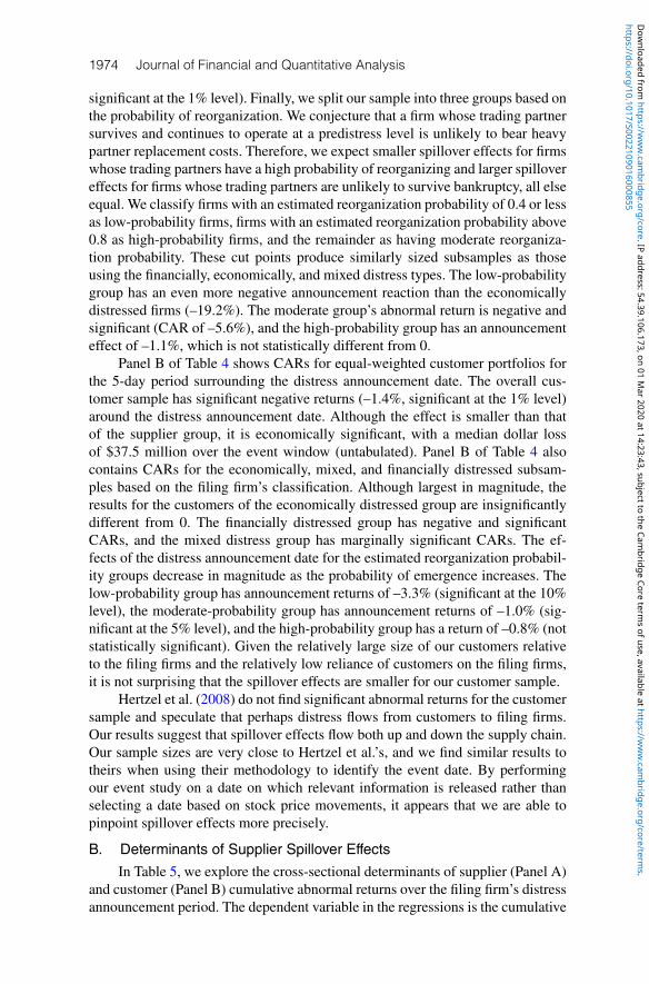
standalone firm using the logistic model from Lemmon et al. (2009). Means andmedians for the variables used in our tests are presented in Table 2. We computeindustry-adjusted operating income based on the EBITDA-to-assets ratio usingthe same industry adjustment as in the proxy for the degree of economic distress.The model also uses Lemmon et al.’s (2009) proxy for the degree of economicdistress described earlier. We use an industry-distress indicator variable that issimilar to that used by Acharya, Bharath, and Srinivasan (2007) and Lemmonet al. (2009) in the logistic regression. We compute the industry-median (based on4-digit SIC code) stock return for the 12 months immediately prior to the Chap-ter 11 filing. If there are fewer than five firms in that 4-digit SIC code, we usethe 3-digit (or, if required, 2-digit) SIC code to calculate the industry median. In-dustries with median returns lower than –30% are identified as distressed, withthe industry-distress indicator variable equal to 1, and 0 otherwise. Eighty-two(30.5%) firms in our sample of filing firms are in a distressed industry. The modelalso incorporates a control for the effects of economic downturns. A recessionindicator variable is set to 1 if the sample firm filed for bankruptcy in a year inwhich the percentage change in gross domestic product (GDP) was in the bottomquartile of GDP changes over our sample period. In our sample, these years are1980, 1982, 1991, and 2009. Finally, the ratio of the filing firm’s R&D expensesto assets is used as a measure of the manager’s information advantage in Chapter11.7 Table 3 contains two models for computing the probability of reorganiza-tion. Model 1 uses the variable for the degree of economic distress, and model 2uses the components of the degree of economic distress (industry-adjusted oper-ating performance and leverage) separately. Both models are significant at the 1%level. The model incorporating the degree of economic distress fits slightly better,so we use that version in our subsequent tests. Overall, 60% of our filing firmsreorganize. Individual estimated probabilities of reorganization from the modelvary considerably and range between 13.7% and 95.5%. Figure 2 presents thedistribution of estimated probabilities using model 1 in Table 3.

7The ratio of R&D expenses to assets is being used as two different proxies: following Lemmonet al. (2009), we use the ratio of R&D to sales of the filing firm as a measure of the manager’s informa-tion advantage for the filing firms. We also use it later as a measure of the product specialization of thesupplier or customer of the filing firm. Although the results presented are from using R&D as a vari-able in our logit regression, we drop this variable because it is insignificant and redo all tests. Resultsremain virtually unchanged. Further, these two are not contradictory, because product specializationimplies uniqueness of goods produced, in which situation managers would have more firm-specificinformation than others.

https://doi.org/10.1017/S0022109016000855D

ownloaded from

https://ww

w.cam



ww


s .

https://doi.org/10.1017/S0022109016000855




TABLE 3Logistic Regressions for the Probability of Reorganization in Chapter 11

Table 3 presents the results from the binomial logistic regressions of Lemmon et al. (2009) where the dependent variableequals 0 if the outcome of Chapter 11 is either liquidation or acquisition (‘‘Liquid/M&A’’) and equals 1 if the outcome isreorganization (‘‘Reorganize’’). PRE_FILING_INDUSTRY_ADJUSTED_OPERATING_PERFORMANCE is measured as theEBITDA-to-assets ratio of the sample firm minus the industry-median ratio of EBITDA to total assets averaged over year–3 and year –2 where both years are available. Year –1 is the fiscal year-end prior to the Chapter 11 filing. The industryis defined at the 4-digit SIC level, provided that it contains a minimum of five firms. Otherwise, the industry is defined atthe 3-digit or 2-digit SIC level. PRE_FILING_LEVERAGE is measured by the ratio of total liabilities to total assets; the ratiois averaged over year –3 and year –2 where data for both years are available. We proxy for the degree of economic (vs.financial) distress using a measure that is constructed similarly to that of Lemmon et al. (2009) by 1) averaging the firm’syear –3 and year –2 industry-adjusted ratio of EBITDA to assets and ranking this into deciles among all Chapter 11 samplefirms, 2) averaging the firm’s year –3 and year –2 leverage and ranking this into deciles among all Chapter 11 samplefirms, and 3) summing these two decile rankings. DEGREE_OF_ECONOMIC_DISTRESS takes on values from 0–18, withhigh values having a higher degree of financial distress and low values having a higher degree of economic distress. Theindustry-adjusted EBITDA-to-assets ratio is the average of the sample firm’s year –3 and year –2 ratio of EBITDA to totalassets minus the industry-median ratio of EBITDA to total assets where both years are available. INDUSTRY_DISTRESS isan indicator variable that equals 1 if the stock return of the median firm in the industry is less than –30% in the 12 monthsimmediately prior to Chapter 11 filing. LOW_GDP_YEARS equals 1 if the firm filed for Chapter 11 in any of the yearsthat comprise the lowest quartile of GDP growth over our sample period. R&D_TO_ASSETS is the ratio of R&D expenseto total assets, is averaged over year –3 and year –2 prior to filing, and is used to capture management’s informationadvantage. Industry dummy variables are based on the Fama–French (1997) 12-industry specification. The z-statisticsfor individual coefficients are reported in parentheses. *, **, and *** indicate significance at the 10%, 5%, and 1% levels,respectively.

Liquid/M&A = 0 Liquid/M&A = 0Reorganize = 1 Reorganize = 1

Variable (Model 1) (Model 2)

Intercept −2.632 −2.748(−2.79)*** (−2.75)***

PRE_FILING_INDUSTRY_ADJUSTED_OPERATING_PERFORMANCE 2.569(1.56)

PRE_FILING_LEVERAGE 1.341(2.31)**

DEGREE_OF_ECONOMIC_DISTRESS 0.123(3.44)***

SIZE (log(TOTAL_ASSETS)) 0.310 0.323(2.56)*** (2.68)***

INDUSTRY_DISTRESS −0.592 −0.554(−1.83)* (−1.71)*

LOW_GDP_YEARS 0.382 0.368(0.88) (0.85)

R&D_TO_ASSETS −2.734 −2.547(−0.66) (−0.54)

Industry dummy variables Yes YesNo. of obs. 269 269Probability >χ2 0.0005 0.0014

C. Distress Announcement DateVery few Chapter 11 filings come as a surprise because most firms try to

avoid bankruptcy by restructuring their assets and liabilities. Chapter 11 is of-ten the final step in the resolution of distress (Asquith, Gertner, and Scharfstein(1994)). Hertzel et al. (2008), who also investigate wealth effects in the supplychain, define the pre-filing distress date as the day during the 12 months priorto bankruptcy on which the filing firm has the largest abnormal dollar loss. Theabnormal dollar loss is measured as the filing firm’s return less the CRSP value-weighted index return multiplied by the market capitalization of the filing firm onthe previous day. This method can have several drawbacks.

First, there is no guarantee that any new information about the firm was re-leased on the Hertzel et al. (2008) date.8 Second, if there is new information about

8Hertzel et al. (2008) examine some of their dates manually and verify that these reflect filing-firm-specific events such as debt downgrades, earnings warnings, and missed earnings expectations.

https://doi.org/10.1017/S0022109016000855D

ownloaded from

https://ww

w.cam



ww


s .

https://doi.org/10.1017/S0022109016000855




FIGURE 2Distribution of Probability of Reorganization Estimates

Figure 2 shows the distribution of reorganization probabilities for our sample of 269 bankruptcy filings estimated usingthe model by Lemmon et al. (2009). Data for estimating the probability include financial data from the fiscal year-end 2and 3 years prior to the Chapter 11 filing, industry dummies, and indicator variables for industry distress and low GDPin the filing year. The model and specific variables are discussed in model 1 of Table 3.

50

45

40

35

30

25

20

15

10

5

0

Freq

uenc

y

≤ 0.16 0.16-0.24 0.24-0.28 0.28-0.32 0.32-0.40 0.40-0.56 0.56-0.64 0.64-0.72 0.72-0.80 0.80-0.88 0.88-0.96

Estimated Probability of Reorganization

the firm, it may not be unambiguously indicative of distress. The Hertzel et al.method of determining the distress date is associated with earnings announce-ments in 25 filing firms in our sample (9%).9 Third, this procedure may select adate on which a firm experiences a spike in its stock price and the price revertson the following day, because the high market capitalization of the day before canlead to very large dollar losses for the following day. Finally, many firms ceasetrading well in advance of a Chapter 11 filing, resulting in incomplete data.10

Perhaps for these reasons, Hertzel et al. report an average abnormal return tosuppliers on their value-loss date of less than half the magnitude of their reportedabnormal return on the Chapter 11 filing date, and the spillover effect is signif-icant at only the 10% level. In this study, we use a date on which informationindicating that the filing firm is in distress is released. Other authors have usedsimilar approaches for identifying key dates in financial distress. Gilson, John,and Lang (1990) and Tashjian, Lease, and McConnell (1996) identify the date onwhich distressed restructurings start as the date of the first announcement that thefirm is renegotiating with creditors, has already renegotiated, or has defaulted.

To identify our distress date, we search for news articles in LexisNexis overthe 1-year period prior to the filing date for each firm.11 From these articles, wechoose (in order) the following categories: 1) any news mentioning suppliers or

However, when their date identification method is implemented in our sample of filing firms that havereturn data on this date and have at least one supplier, we find 10 filing firms for which we are unableto find any new information released on or near (–1 to +1) that date.

9Filing firms are limited to those that have return data on this date and at least one supplier.10Furthermore, Hertzel et al. (2008) select their event date based on a date of maximum market cap

loss, making it difficult to determine whether any negative abnormal returns they find are the result ofspillover effects or are an outcome of their sample construction process.

11In three filings, it was clear that the market knew of distress prior to the 1-year period beforefiling. In these three cases, the distress announcement date occurs more than 12 months before thefiling date. We ensure that the financial data used to calculate the probability of reorganization forthese three firms are known before the news date.

https://doi.org/10.1017/S0022109016000855D

ownloaded from

https://ww

w.cam



ww


s .

https://doi.org/10.1017/S0022109016000855




customers of the filing firm explicitly responding to the distress in the tradingpartner (e.g., suppliers refusing to extend credit or customers requiring extra war-ranties); 2) news regarding a failed restructuring attempt, news that the firm isunlikely to recover, or news that the firm is facing distress and will likely failif restructuring or refinancing does not occur; 3) news that a firm has hired anadvisory or investment firm for potential restructuring, fails to make debt pay-ments, or receives a going-concern qualification by its auditor; and finally, 4) anyannouncement of an attempt at asset restructuring, such as asset sales, mergers,capital expenditure reductions, and layoffs, or an attempt at debt restructuring. Ifmultiple items in any category are available, we take the earliest. For brevity, werefer to these types of news items as 1) trading partner reaction, 2) failure likely,3) distress onset, and 4) restructuring.

Suppliers and customers have a direct motive to monitor their trading part-ners. In addition to the loss of future profits, suppliers may also lose any unpaidtrade credit. Trade-credit theories posit that this leads sellers to have an incentiveto monitor the (filing) customer firm (Smith (1987), Brennan, Maksimovic, andZechner (1988), Petersen and Rajan (1997), Biais and Gollier (1997), and Burkartand Ellingsen (2004)). Therefore, direct information pertaining to trading partnersis our first choice. Choosing dates with news about suppliers or customers givesrise to the concern that announcement effects for suppliers and customers maybe driven by information about these firms rather than the distressed customers.However, we find that less than 7% of our dates for the entire sample of filingfirms belong to the first category. Our results remain virtually unchanged whenwe exclude these observations from our subsequent analysis.

Because many suppliers function as short-term creditors to their customers,they may continue to extend credit even if they know that their trading partnersare distressed. Thus, we expect that such suppliers will be affected most stronglywhen they have already stretched themselves in expectation that their trading part-ners will restructure successfully and the restructuring fails. In the absence of thefirst two criteria, we select news that reflects the onset of distress, such as misseddebt payments or hiring an advisory firm for restructuring. We use these becausethey either appear before any restructuring attempts are made or are the very firststeps in the restructuring process. As our last choice, we pick those news storiesthat indicate that an attempt at asset or liability restructuring has been made, be-cause these do not constitute unambiguously bad news for the trading partners.In the occasional case where there is no reported attempt at a restructuring beforefiling, we use the filing or the filing announcement as the onset of distress.

For the sample of bankrupt firms that have one or more suppliers, the datesare distributed across groups as follows: supplier reaction, 8%; failure likely,30%; distress onset, 36%; restructuring, 14%; and for 11%, we use the filingdate. Correspondingly, for the sample of bankrupt firms that have one or morecustomers, the dates are distributed between the category types as follows: cus-tomer reaction, 5%; failure likely, 17%; distress onset, 57%; restructuring,13%;and for 8%, we use the filing date. We also repeat the date choice process for oursubsample of Chapter 11 filings for which we can identify the date when the pos-sibility of bankruptcy was first mentioned specifically by the distressed firm itself

https://doi.org/10.1017/S0022109016000855D

ownloaded from

https://ww

w.cam



ww


s .

https://doi.org/10.1017/S0022109016000855




or by analysts or other market participants (and not suppliers to the filing firm).12

We find that our regression estimates remain qualitatively unchanged.We are able to compare our information-based distress dates (henceforth, the

“distress announcement date”) to the date in Hertzel et al. (2008) (henceforth, the“value-loss date”) for 188 firms in our sample.13 Of those firms for which we areable to identify the value-loss date, 145 (77%) have value-loss dates that precedeour information-based distress announcement dates, 19 firms (10%) have distressannouncement and value-loss dates that coincide, and 24 (13%) have value-lossdates that occur later than the distress announcement date. On average (median),Hertzel et al.’s value-loss date occurs 99 (96) days before our distress announce-ment date. As firms move toward bankruptcy, their market capitalization becomessmaller as a result of falling stock prices, which tends to lead to earlier value-lossdates.

IV. Determinants of Spillover Effects in the Supply Chain

A. Distress Announcement Abnormal Returns to Suppliersand CustomersAverage distress announcement and filing-period cumulative abnormal re-

turns to suppliers over a 5-day window centered on the distress announcementand the Chapter 11 filing date are presented in Table 4, Panel A. We computeabnormal returns using the market-adjusted returns method (Brown and Warner(1985)), in which the daily abnormal return is the firm-specific return minus theCRSP value-weighted market return. For each filing company, we form equal-weighted portfolios of all its suppliers. The average supplier return is the simpleaverage of these portfolio returns. The abnormal return is –7.3% on the distressannouncement date, which is significantly different from 0 at the 1% level. Weobtain a cumulative abnormal return (CAR) of –1.7% (significant at the 1% level)for the CAR around the value-loss date.

Table 4 also presents subsample results for Lemmon et al.’s (2009) classi-fication into economically, mixed, or financially distressed firms. As the distresstype changes from economic to financial, the abnormal returns decrease in mag-nitude. The CAR for the 5-day distress announcement period is a statisticallysignificant−12.3% for economically distressed firms, whereas for financially dis-tressed firms, the CAR is an insignificant –0.8%.14 The corresponding CARs forthe value-loss period (not tabulated) are –2.7% and 5.7% (both insignificant). Thedistress announcement date CAR for the mixed type of distressed firms are inthe middle, with a significant –7.5% CAR (–4.5% during the value-loss period,

12We focus on the filing firms that have suppliers because in our data, customers of filing firmsseldom have any news related to their distressed suppliers. All of our dates in this category involvesuppliers rather than customers.

13Stock prices are unavailable for many firms in the period leading up to a Chapter 11 filing,precluding identifying the value-loss date.

14In this and subsequent panels where we divide the sample by distress type or probability of reor-ganization, we eliminate extreme outliers because the subsamples are small. This results in eliminatinga total of between 0 and 3 outliers across all three subsamples, depending on the table. (The largestnumber of outliers in any subgroup is 2.)

https://doi.org/10.1017/S0022109016000855D

ownloaded from

https://ww

w.cam



ww


s .

https://doi.org/10.1017/S0022109016000855



Kolay,Lem

mon,and

Tashjian1973

TABLE 4CARs to Suppliers and Customers of Bankrupt Firms over Distress Announcement Date

Table 4 contains average distress-period supplier and customer CARs. We identify suppliers and customers by examining firms reporting major customers in Compustat segment data in the 5 years priorto sample firms’ Chapter 11 filings. We form equal-weighted customer and supplier portfolios from the individual customers and suppliers for each filing. The distress day is the first date with major news offinancial distress in the 12 months prior to filing. Additional details are given in Section III. Suppliers and customers are grouped into distress type using the measure for the degree of economic distress.We proxy for the degree of economic (vs. financial) distress using a measure that is constructed similarly to that of Lemmon et al. (2009), as described in Table 3, or by the probability of reorganizationbased on model 1 in Table 3. Firms with a reorganization probability of less than or equal to 0.40 are classified as low-probability firms, firms with a reorganization probability of 0.80 or higher are classifiedas high-probability firms, and the remaining firms are classified as moderate-probability firms. The abnormal returns are cumulated for days −2 to +2 relative to the distress announcement date, and dailyabnormal returns are calculated using market-adjusted returns (MARs) with the CRSP value-weighted index as the market index. Standard errors are computed as described by Patell (1976). *, **, and ***indicate that the average is significantly different from 0 (using a 2-sided t -test) at the 10%, 5%, and 1% levels, respectively.

Panel A. Supplier Average CARs for Distress Announcement Date

By Filing Firm Distress Type By Probability of Reorganization Type

Suppliers to Suppliers to Suppliers to Suppliers to Suppliers to Suppliers toEconomically Mixed Financially Low- Moderate- High-Distressed Distressed Distressed Probability Probability Probability

Full Sample Firms Firms Firms Firms Firms Firms

Average CAR (−2, +2) −7.30%*** −12.27%*** −7.54%*** −0.77% −19.19%*** −5.56%*** −1.12%No. of equal-weighted portfolios (122) (21) (82) (19) (22) (80) (20)

Panel B. Customer Average CARs for Distress Announcement Date

By Filing Firm Distress Type By Probability of Reorganization Type

Customers to Customers to Customers to Customers to Customers to Customers toEconomically Mixed Financially Low- Moderate- High-Distressed Distressed Distressed Probability Probability Probability

Full Sample Firms Firms Firms Firms Firms Firms

Average CAR (−2, +2) −1.36%*** −2.02% −1.04%* −1.51%** −3.25%* −1.00%** −0.77%No. of equal-weighted portfolios (150) (26) (98) (26) (24) (101) (25)

https://doi.org/10.1017/S0022109016000855Downloaded from https://www.cambridge.org/core. IP address: 54.39.106.173, on 01 Mar 2020 at 14:23:43, subject to the Cambridge Core terms of use, available at https://www.cambridge.org/core/terms.

https://doi.org/10.1017/S0022109016000855




significant at the 1% level). Finally, we split our sample into three groups based onthe probability of reorganization. We conjecture that a firm whose trading partnersurvives and continues to operate at a predistress level is unlikely to bear heavypartner replacement costs. Therefore, we expect smaller spillover effects for firmswhose trading partners have a high probability of reorganizing and larger spillovereffects for firms whose trading partners are unlikely to survive bankruptcy, all elseequal. We classify firms with an estimated reorganization probability of 0.4 or lessas low-probability firms, firms with an estimated reorganization probability above0.8 as high-probability firms, and the remainder as having moderate reorganiza-tion probability. These cut points produce similarly sized subsamples as thoseusing the financially, economically, and mixed distress types. The low-probabilitygroup has an even more negative announcement reaction than the economicallydistressed firms (–19.2%). The moderate group’s abnormal return is negative andsignificant (CAR of –5.6%), and the high-probability group has an announcementeffect of –1.1%, which is not statistically different from 0.

Panel B of Table 4 shows CARs for equal-weighted customer portfolios forthe 5-day period surrounding the distress announcement date. The overall cus-tomer sample has significant negative returns (–1.4%, significant at the 1% level)around the distress announcement date. Although the effect is smaller than thatof the supplier group, it is economically significant, with a median dollar lossof $37.5 million over the event window (untabulated). Panel B of Table 4 alsocontains CARs for the economically, mixed, and financially distressed subsam-ples based on the filing firm’s classification. Although largest in magnitude, theresults for the customers of the economically distressed group are insignificantlydifferent from 0. The financially distressed group has negative and significantCARs, and the mixed distress group has marginally significant CARs. The ef-fects of the distress announcement date for the estimated reorganization probabil-ity groups decrease in magnitude as the probability of emergence increases. Thelow-probability group has announcement returns of –3.3% (significant at the 10%level), the moderate-probability group has announcement returns of –1.0% (sig-nificant at the 5% level), and the high-probability group has a return of –0.8% (notstatistically significant). Given the relatively large size of our customers relativeto the filing firms and the relatively low reliance of customers on the filing firms,it is not surprising that the spillover effects are smaller for our customer sample.

Hertzel et al. (2008) do not find significant abnormal returns for the customersample and speculate that perhaps distress flows from customers to filing firms.Our results suggest that spillover effects flow both up and down the supply chain.Our sample sizes are very close to Hertzel et al.’s, and we find similar results totheirs when using their methodology to identify the event date. By performingour event study on a date on which relevant information is released rather thanselecting a date based on stock price movements, it appears that we are able topinpoint spillover effects more precisely.

B. Determinants of Supplier Spillover EffectsIn Table 5, we explore the cross-sectional determinants of supplier (Panel A)

and customer (Panel B) cumulative abnormal returns over the filing firm’s distressannouncement period. The dependent variable in the regressions is the cumulative

https://doi.org/10.1017/S0022109016000855D

ownloaded from

https://ww

w.cam



ww


s .

https://doi.org/10.1017/S0022109016000855




abnormal return around the distress announcement date of individual suppliers(Panel A) or individual customers (Panel B). Because the individual suppliers toor customers of a particular filing customer are not independent, the t-statisticspresented are based on clustered standard errors that control for clustering byindustry and the month of the year.15

TABLE 5Cross-Sectional Determinants of CARs to Suppliers and Customers of Bankrupt Firms

Table 5 consists of ordinary least squares (OLS) regressions where the dependent variable is the CAR to suppliers(Panel A) and customers (Panel B) of firms that file for bankruptcy. The CARs are calculated over a 5-day periodcentered on the distress announcement date. SUPPLIER_LEVERAGE is calculated as the average of the supplier’sratio of total liabilities to total assets at year –1 and year –2 relative to filing. SUPPLIER_R&D_INTENSITY is R&D ex-penses/total assets for each supplier calculated as the average ratio of R&D expenses to total assets at year –1 andyear –2 relative to filing. FILING_CUSTOMER_INDUSTRY_CONCENTRATION is the Herfindahl index calculated for eachfiling firm using all the firms in the same 4-digit SIC code, and SUPPLIER_INDUSTRY_CONCENTRATION is computedsimilarly. FILING_CUSTOMER_PROBABILITY_OF_REORGANIZATION is taken from the predicted values of the logis-tic regression presented in model 1 of Table 3. %_SALES_FROM_DISTRESSED_CUSTOMER is computed as suppliersales generated from the filing firm in the year in which the relationship is identified between the firms scaled by thetotal sales of the supplier in that year. SUPPLIER_RECEIVABLES_FROM_DISTRESSED_CUSTOMER (Panel A) are es-timated by multiplying the percentage of the supplier’s sales generated by the filing customer by the average tradereceivables in year –2 and year –1 relative to filing, and customer payables are computed analogously (Panel B).SUPPLIER_INDUSTRY_ABNORMAL_RETURN (Panel A) and CUSTOMER_INDUSTRY_ABNORMAL_RETURN (Panel B)are calculated using all firms in the same 3-digit SIC code as the relevant supplier or customer, excluding the samplefirm. The t-statistics reported in parentheses control for clustering effects resulting from supplier industry and month ofthe year. *, **, and *** indicate significance at the 10%, 5%, and 1% levels, respectively. The dependent variable is thesuppliers’ (Panel A) or customers’ (Panel B) CAR for days –2 to +2 relative to the distress date of the bankrupt firm andis calculated using MARs with the CRSP value-weighted index as the market index.

Panel A. Suppliers to Bankrupt Firms

Dependent Variable: CAR from (–2, +2) for Individual Suppliers around the Distress Announcement Date

Model

Variable 1 2 3 4 5 6 7

Intercept −0.199 −0.174 −0.120 −0.054 −0.132 −0.165 −0.122(−3.51)*** (−3.12)*** (−2.06)** (−4.12)*** (−2.07)** (−2.60)*** (−2.03)**

FILING_CUSTOMER_PROBABILITY_ 0.214 0.234 0.240 0.231 0.224 0.241OF_REORGANIZATION (2.82)*** (3.08)*** (3.56)*** (3.00)*** (3.21)*** (3.46)***

%_SALES_FROM_DISTRESSED_CUSTOMER −0.265 −0.274 −0.259 −0.247(−6.55)*** (−5.87)*** (−5.92)*** (−3.91)***

SUPPLIER_R&D_INTENSITY −0.176 −0.174 −0.210 −0.180(−3.67)*** (−3.07)*** (−3.21)*** (−3.43)***

FILING_CUSTOMER_INDUSTRY_ 0.054 0.065 0.060 0.048CONCENTRATION (1.33) (1.31) (1.50) (1.17)

SUPPLIER_INDUSTRY_CONCENTRATION −0.057 −0.040 −0.039 −0.053(−2.00)** (−1.06) (−1.05) (−1.68)*

SUPPLIER_LEVERAGE 0.003 0.021 0.002 0.001(0.09) (0.68) (0.07) (0.03)

SUPPLIER_SIZE −0.010 −0.009 −0.007 −0.010(−2.52)** (−1.99)** (−1.63)* (−2.36)**

SUPPLIER_INDUSTRY_ 0.677 0.409ABNORMAL_RETURN (1.55) (1.41)

SUPPLIER_RECEIVABLES_FROM_ −0.051 −0.026DISTRESSED_CUSTOMER (−5.68)*** (−1.74)*

No. of obs. 270 262 262 240 233 251 251p-value of F-statistic <0.0001 <0.0001 <0.0001 0.004 <0.0001 <0.0001 <0.0001Adj. R 2 0.083 0.149 0.171 0.030 0.176 0.123 0.170


15Industry is defined as 2-digit SIC code. Month of the year is used so that all suppliers for aparticular bankruptcy are clustered because the filing date is the same for all. We repeat the analysisby forming portfolios of all suppliers for each filing firm and repeat the analysis again with firm-level

https://doi.org/10.1017/S0022109016000855D

ownloaded from

https://ww

w.cam



ww


s .

https://doi.org/10.1017/S0022109016000855




TABLE 5 (continued)Cross-Sectional Determinants of CARs to Suppliers and Customers of Bankrupt Firms

Panel B. Customers of Bankrupt Firms

Dependent Variable: CAR from (−2, +2) for Individual Customers of Filing Firms around the Distress Announcement Date

Model

Variable 1 2 3

Intercept −0.037 −0.011 −0.023(−1.29) (−1.77)* (−0.90)

FILING_SUPPLIER_PROBABILITY_OF_REORGANIZATION 0.003 −0.002(0.11) (−.008)

%_PURCHASES_FROM_FILING_SUPPLIER −0.069 −0.066(−2.89)*** (−3.65)***

CUSTOMER_R&D_INTENSITY −0.446 −0.387(−7.32)*** (−7.49)***

FILING_SUPPLIER_INDUSTRY_CONCENTRATION 0.012 0.019(0.80) (1.33)

CUSTOMER_INDUSTRY_CONCENTRATION 0.001 0.004(0.03) (−0.20)

CUSTOMER_LEVERAGE 0.002 −0.013(0.10) (−0.73)

CUSTOMER_SIZE 0.003 0.003(1.36) (1.53)

CUSTOMER_INDUSTRY_ABNORMAL_RETURN 0.318 0.319(2.44)** (2.52)**

No. of obs. 273 281 264p-value of F-statistic <0.0001 <0.0001 <0.0001Adj. R 2 0.181 0.049 0.222

Model 1 in Table 5 examines the impact of the probability of reorganiza-tion (from model 1 in Table 3) on CARs around the distress announcement date.The estimated coefficient on the probability of reorganization is positive and botheconomically and statistically significant. A 10% lower probability of reorganiza-tion is associated with a 2% drop in the CAR over the 5-day period. Multiplyingthe coefficient by the median market capitalization of the supplier firm sampletranslates to an approximate loss of $24.5 million ($185 million mean) over 5days for a representative firm. The model suggests that if the bankrupt firm has asufficiently high probability of reorganizing successfully, its supplier may not ex-perience any negative wealth effects: the intercept is –0.20, and the coefficient onthe reorganization probability is 0.21. The sum of these coefficients is statisticallyindistinguishable from 0. In model 2, we add our proxy for the level of supplierdependence on a bankrupt customer. The estimated coefficient for the percent-age of sales generated by the filing customer is strongly negative and significant.Together, our measures of the probability of reorganization and reliance explainnearly 15% of the variation in abnormal returns.

Model 3 of Table 5, our base model, adds the other independent variablesdesigned to capture expected partner replacement costs.16 The coefficient of R&D

fixed effects for filing firms with at least five suppliers. The results are a bit weaker given the reducedsample size but qualitatively similar.

16If the suppliers are themselves operating in distressed industries, it may magnify the impact of apartner’s distress. In addition to the results here, we also add an indicator for the filing firm’s distressto our base specification (model 3) and an analogously defined distress indicator for the nonfiling sup-

https://doi.org/10.1017/S0022109016000855D

ownloaded from

https://ww

w.cam



ww


s .

https://doi.org/10.1017/S0022109016000855




intensity is significant and negative. This is consistent with the evidence providedby Titman and Wessels (1988) and Banerjee et al. (2008): a higher level of productspecialization and the consequent higher level of relationship-specific investmentsin the trading relationship lead to greater costs in switching to a new partner. Wefind evidence that the supplier’s industry concentration affects its abnormal re-turns. As hypothesized in the previous section, the more competitive the supplier’sindustry, the more negative the wealth effect on the supplier. We add the supplier’slog of total assets to control for any size effects and find that the larger the firm, themore negative the CAR. Neither the distressed customer’s industry concentrationnor supplier leverage is statistically significant in explaining the CARs tosuppliers.

In unreported results, we repeat models 1 through 3 of Table 5, replacing theprobability of reorganization with Lemmon et al.’s (2009) measure of the degreeof economic distress. In all three regressions, the coefficient is positive and signif-icant, indicating that more financially distressed firms impose fewer costs on theirtrading partners. However, the R2 values of the regressions are substantially lowerthan those for the comparable regressions using the probability of distress, and inmodel 1, the intercept does not equal the coefficient on the variable for the degreeof distress. Although the degree of distress is an important factor in our estimatesof the likelihood of reorganizing, it appears that the probability of reorganizationof the distressed firm is a better predictor of the market’s response to the distressannouncement, reinforcing our hypothesis that expected replacement costs are akey driver of spillover effects.

Model 4 of Table 5 looks at the information effect alone, and model 5 addsour proxy for information to the base model. Although the coefficients on theindustry-abnormal return are positive, they are not statistically significant in eitherregression (t-statistics of 1.55 and 1.41, respectively). Although we control forindustry effects, it is possible that the information is specific to the web of firmsin a particular supply chain. We repeat model 5 for the subsample of filing firmswith five or more suppliers (not shown in the table). This subsample consists of 17filing firms and 131 suppliers. For each supplier, we replace the industry-abnormalreturn with the abnormal return for all other suppliers for the associated filing firmin our sample, excluding the specific supplier. The coefficient on the probabilityof reorganization becomes insignificant (which is not surprising given that thereare only 17 filing firms); other variables remain significant, and the informationvariable’s coefficient is still insignificant. Thus, the abnormal return to suppliersaround the distress announcement date appears to be explained in the cross sectionby the expected cost of replacing the distressed partner rather than by information.

Finally, we examine whether the negative CARs surrounding the bankruptfirm’s distress date can be explained by its supplier’s own outstanding trade re-ceivables to explore whether credit costs are an important determinant of spillovercosts. The potential loss to the supplier is equal to the losses attributable to past

plier’s industry. We find that, in addition to the probability of reorganization, the filing firm’s industrydistress is significant (coefficient: –0.06) but does not reduce the coefficient on the probability of reor-ganization significantly. The indicator for the supplier’s industry distress is insignificant (coefficient:–0.05). Adding both of these leads to an increase of 1.49% in the Adj. R2 value of the regression.

https://doi.org/10.1017/S0022109016000855D

ownloaded from

https://ww

w.cam



ww


s .

https://doi.org/10.1017/S0022109016000855




loans made to the filing customer (in the form of trade credit) plus the presentvalue of future lost sales. In performing our tests, we first calculate a proxy forthe normalized trade receivables outstanding with respect to the filing customeras follows: percentage of supplier’s sales generated from the filing customer ×(supplier’s trade receivables/supplier’s sales).

The results from adding this variable to the base model from model 3 inTable 5 are shown in models 6 and 7. Model 6 includes our proxy for tradecredit but excludes the percentage of sales from the distressed customer, whichforms part of our proxy. The supplier receivables variable is significantly negative(t-statistic of –5.68), but the R2 value of the model drops from 0.17 in our basecase to 0.12. In model 7, the original percentage of the supplier’s sales to the filingcustomer is also included. This accounts for the portion of the loss that the sup-plier expects as a result of the probability of lower future cash flows because oflost sales. As shown in model 7, the total receivables variable is negative but onlymarginally significant (t-statistic = –1.74). The magnitude of the coefficient ofthe total sales percentage to the filing customer variable is now marginally smallercompared with model 3 but is still significant (t-statistic = –3.91). This suggeststhat although higher amounts of receivables due from the filing customer are inter-preted by the market as a weak negative sign, greater losses are anticipated fromexpected partner replacement costs.17

Our relatively weak results for the impact of credit costs compared with thoseof Jorion and Zhang (2009) may be attributable to differences in sample construc-tion. They identify their sample from the 20 largest unsecured creditors at thetime of the Chapter 11 filing. Further, Jorion and Zhang (2009) do not includevariables designed to capture trading partner replacement costs in their regres-sions, so our results are not comparable. We follow Jorion and Zhang (2009) andexamine the list of large unsecured creditors provided by the filing firms in oursample at the time they file for Chapter 11. Typically, the list contains about 20creditors, although firms in our sample list as few as 5 and as many as 100 un-secured creditors. In some cases, the list exclusively consists of banks serving astrustees for various unsecured debt issues. In other cases, the list contains quite afew trade creditors. The list identifies the name of the unsecured creditor, the typeof debt (e.g., public debt or trade credit), and the estimated amount of the claim.Of the 145 bankrupt firms with at least one supplier, we are able to obtain the listof large unsecured creditors for half (73). Of our initial sample of 378 suppliers,202 of them are from firms for which we have a list of large unsecured creditors.Only 12% (24 firms) of these 202 suppliers appear on the list. In Section V.B, weexamine trade-credit losses more directly based on information reported in U.S.Securities and Exchange Commission (SEC) filings.

Trade credit is often treated differently from other unsecured claims in Chap-ter 11. Firms in Chapter 11 typically continue operating and often petition to paysuppliers in the ordinary course of business, making trade credit less vulnerable

17In unreported results, we repeat our baseline model (model 3) using the CARs for the value-lossdate and find insignificant results. We also repeat all of our tests after excluding observations wherethe supplier and filing firm are in similar industries (i.e., where their SIC codes match at the 3- or4-digit level) from our regressions and find that results remain qualitatively unchanged.

https://doi.org/10.1017/S0022109016000855D

ownloaded from

https://ww

w.cam



ww


s .

https://doi.org/10.1017/S0022109016000855




to write-offs than other forms of unsecured credit. Although Franks and Torous(1994) do not report recovery rates for trade creditors, they do report that tradecreditors in Chapter 11 receive 98.6% of their recovery in the form of cash, ascompared with other junior creditors, who receive 10.5% of their recovery incash. Other creditors are not permitted to receive payments during Chapter 11.Thus, Chapter 11’s special treatment of trade creditors is likely to reduce poten-tial spillover costs arising from credit losses significantly.

To summarize, we find that in the cross section, abnormal returns to suppliersare associated strongly with some of our proxies for expected replacement costs,including the probability of reorganization, retooling costs, and the degree of re-liance. In contrast, our proxies for capturing the credit costs and information costsare insignificant, implying that spillover effects in the supply chain generate realreplacement costs and are not just the result of counterparty risk or of the releaseof industry information.

C. Determinants of Customer Spillover EffectsPanel B of Table 5 presents the results of tests for the cross-sectional determi-

nants of the distress announcement date CARs for our sample of filing firms’ cus-tomers. Model 1 presents our base model for exploring expected firm replacementcosts for individual customers, again using clustered errors. The degree of relianceby the customer on the filing firm and the supplier’s level of product specialization(measured by R&D intensity) are important for downstream contagion, both withnegative and significant coefficients (t-statistics of –2.90 and –7.32, respectively).It appears that the switching costs attributable to product specialization are one ofthe main drivers of the contagion effects on the customer. Customers who are notreliant on the filing suppliers in terms of their percentage of purchases may stillface substantial retooling costs as a result of technological dependence on theirsuppliers.18 The other coefficients are not statistically significant.

Although Panel B of Table 4 suggests that the probability of reorganization isan important determinant of abnormal returns for customers, once we account forthe other explanatory variables, the probability of reorganization is not significant,in contrast to its effect on suppliers to distressed firms. A supplier may not havean alternative outlet for its existing goods or services, so losing a key customermay require a substantial effort to replace the distressed partner or even requireretooling for a different trading partner. On the other hand, customers of failedfirms can presumably pay another firm to deliver similar inputs: the change mayraise costs, and those costs are likely to be worse if its supplier is in a concentratedindustry and it is purchasing company-specific products. The asymmetric impacton suppliers and customers of losing a trading partner may partially explain thelower announcement effect we observe for customers.

Model 2 of Table 5 looks at information effects alone. In contrast to the sup-pliers, customers of filing firms do show significant information effects. Whenwe include our information proxy along with the variables that proxy for replace-

18Ellis, Fee, and Thomas (2012) find that customers reporting significant trading partners (on whichour sample is based) tend to be those with lower R&D expenses. They conjecture that firms with sub-stantial proprietary information may underreport trading partners. Thus, product specialization maybe more important than our results suggest.

https://doi.org/10.1017/S0022109016000855D

ownloaded from

https://ww

w.cam



ww


s .

https://doi.org/10.1017/S0022109016000855




ment costs (model 3), the replacement cost variables retain their same significanceas in model 1, and the information variable is positive and significant (t=2.52).Therefore, spillover effects in customers of filing firms are not driven solely byreplacement costs.

V. Supplier Performance around BankruptcyIn this section, we explore what happens to suppliers following the dis-

tress announcement. We focus on two aspects of supplier outcomes and examinewhether changes in realized operating performance following bankruptcy appearto be tied to determinants of spillover effects, and we explore whether suppliersappear to adjust their trade-credit policies both leading up to and in Chapter 11 inresponse to the distress of their trading partners.

A. Realized Supplier Operating PerformanceTo calculate performance changes for suppliers, we use a matched firm

adjustment approach, following Barber and Lyon (1996) and Fee and Thomas(2004). Each supplier to a filing firm is matched with a control firm chosen onthe basis of industry, asset size, and operating performance in the pre-filing year.Starting with the entire universe of Compustat firms, we eliminate all bankruptfirms and their suppliers and customers. From the remaining firms, we identifythose in the same 2-digit SIC code with an asset size at the end of the year priorto bankruptcy that is between 25% and 200% of the supplier’s and an operatingprofit percentage that is between 90% and 110% of the supplier’s. From the setof these possible matches, we choose the one closest in operating performance tothe supplier. If matches are not found at this stage, the industry screen is relaxedto a 1-digit SIC match requirement. At the next stage, the industry-matching re-quirement is removed, and matches are made only on the basis of asset size andperformance. If we are still left with no match, we use the operating-performancematching only at the last stage. If the matched firm drops out, it is replaced withthe next best available match. There is attrition in our sample each year becausenot all suppliers have more than one match using the most relaxed matching cri-teria, and not all suppliers have data for all years on Compustat.19 We are able tofind 200 supplier-matched firm pairs by this process in the year prior to customerbankruptcy. We follow the performance of the sample of suppliers relative to thatof their matching firms from the year prior to filing to 3 years after filing. Ouraim is to investigate whether supplier pre-filing spillover effects translate into lostsales, increased costs, or overall declining margins.

Table 6 presents several matched-firm-adjusted financial measures for sup-pliers beginning at time –1, the fiscal year-end prior to the Chapter 11 filings oftheir distressed partners. The table also reports year-over-year changes in thosemeasures for the subsequent 4 years. The change in the match-adjusted sales-to-assets ratio is negative but insignificant from year 0 (the first fiscal year followingthe Chapter 11 filing) to year 1. Changes in the ratio of cost of goods sold to

19As a check for survivorship bias in our results for this section, we fix all firms that have data inyear+3 after the filing (varies from 102 to 83 depending on the particular variable) and redo our tests.Although significance is diminished in these tests, the trends remain the same.

https://doi.org/10.1017/S0022109016000855D

ownloaded from

https://ww

w.cam



ww


s .

https://doi.org/10.1017/S0022109016000855




TABLE 6Operating Performance of Suppliers Following the Distress Date

Table 6 presents the match-firm-adjusted measures of operating performance for suppliers to filing firms. Each value isa difference found by subtracting the variable value of the corresponding matching firms. Matching firms are calculatedusing the Barber and Lyon (1996) method by choosing those matched firms that are closest to each sample supplierfirm by industry (2-digit SIC code), size (25%–200% of assets), and operating performance (year prior to bankruptcyannouncement). The variable changes from year n−1 to year n are the difference of each measure between the values inthe corresponding years. Year 0 is the fiscal year-end following the bankruptcy filing (see definition of timing convention inSection III). Operating profit is defined as EBITDA. Altman’s z-score is fromAltman (1968). Panel C presents the regressionof match-firm-adjusted operating performance and SG&A expenses for suppliers to filing firms. The dependent variableis the change in the match-firm-adjusted operating performance or SG&A of the suppliers from the pre-filing fiscal year-end (year –1) and the fiscal year-end of the following filing year (year 0). Independent variables are described in Table 5.The p-values (reported in parentheses in Panels A and B) are calculated from t -tests for the means and from Wilcoxonranked-sum tests for the medians. The t -statistics reported in parentheses in Panel C control for clustering. *, **, and ***indicate significance at the 10%, 5%, and 1% levels, respectively.

Panel A. Match-Firm-Adjusted Revenue, COGS, and Gross Profit Following the Distress Date

Sales/Assets COGS/Assets Gross Profit/Sales

No. of Obs. Mean Median No. of Obs. Mean Median No. of Obs. Mean Median

Value in year –1 200 −0.089 0.056* 200 −0.085 0.031** 200 −0.004 0.000

Change from year –1 to year 0 198 0.078 −0.003 198 0.095 0.003 198 −0.017 −0.004(0.53) (0.36) (0.44) (0.57) (0.34) (0.35)

Change from year 0 to year 1 146 −0.494 −0.012 146 −0.443 0.005 122 −0.051 −0.012(0.23) (0.76) (0.27) (0.44) (0.02)** (0.11)

Change from year 1 to year 2 130 0.742 0.024 130 0.706 0.012 130 0.035 0.013(0.26) (0.03)** (0.27) (0.13) (0.27) (0.05)**

Change from year 2 to year 3 99 0.057 0.005 99 0.057 0.008 99 0.000 0.002(0.34) (0.67) (0.30) (0.51) (0.99) (0.53)

Panel B. Match-Firm-Adjusted SG&A, Operating Profit, and Altman’s z-Score Following the Distress Date

SG&A/Assets Operating Profit/Assets Altman’s z -Score


Value in year –1 163 −0.007 0.002 200 0.000 0.000 178 −0.378 0.124

Change from year –1 to year 0 161 0.039 0.003 197 −0.049 −0.020 176 −0.017 −0.070(0.01)*** (0.03)** (0.02)** (0.01)*** (0.94) (0.09)*

Change from year 0 to year 1 113 −0.012 0.009 145 −0.021 −0.012 129 −0.859 −0.130(0.75) (0.13) (0.41) (0.11) (0.04)** (0.01)***

Change from year 1 to year 2 99 0.013 −0.002 127 −0.023 0.007 118 0.467 0.073(0.36) (0.99) (0.54) (0.26) (0.49) (0.44)

Change from year 2 to year 3 77 0.027 0.003 94 −0.027 0.008 87 −0.667 −0.009(0.14) (0.35) (0.29) (0.31) (0.04)** (0.61)

Panel C. OLS Regressions of Changes in Match-Firm-Adjusted Operating Profit and SG&A over the Year before Filing to the Yearafter Emergence

Dependent Variable

Variable Change in Operating Profit Change in SG&A

Intercept −0.063 0.146(−0.88) (2.24)**

FILING_CUSTOMER_PROBABILITY_OF_REORGANIZATION 0.189 −0.187(2.11)** (−2.56)***

%_SALES_FROM_DISTRESSED_CUSTOMER −0.152 0.125(−1.59) (1.62)

SUPPLIER_R&D_INTENSITY −0.307 0.234(−0.89) (1.19)

FILING_CUSTOMER_INDUSTRY_CONCENTRATION −0.017 −0.117(−0.29) (−2.60)***

SUPPLIER_INDUSTRY_CONCENTRATION −0.130 0.117(−2.42)** (2.46)**

SUPPLIER_LEVERAGE 0.017 −0.012(1.75)* (−1.35)

SUPPLIER_SIZE −0.010 −0.001(−1.52) (−0.20)

No. of obs. 175 147p-value of F-statistic 0.0246 0.0019Adj. R2 0.052 0.105

https://doi.org/10.1017/S0022109016000855D

ownloaded from

https://ww

w.cam



ww


s .

https://doi.org/10.1017/S0022109016000855




assets are insignificant for all years. Gross profits fall significantly at the meanfrom year 0 to year 1, and they rise significantly at the median from year 1 to year2.20 Although the results in Panel A are not strongly compelling, they do seemto suggest that suppliers to distressed firms (relative to their matched peers) mayhave a drop in sales and profits associated with the bankruptcy filings of theirdistressed partners, followed by a recovery.21

The results in Panel B of Table 6 are more interesting. We find that the SG&Acosts of suppliers increase significantly in the filing year, and correspondingly, weobserve a significant 2% median (5% mean) decline in operating profitability rela-tive to a matched sample. Kalwani and Narayandas (1995) find that those suppliersthat have long-term relationships with their customers spend less on SG&A as aresult of lower service costs, higher repeat sales, and higher overall effectivenessof selling expenditures rather than simply reflecting a decrease in sales.22 Takentogether with our earlier results, the evidence suggests that spillover effects at-tributable to the distress of the filing firm may lead to an erosion of the supplier’scombined efficiencies in selling expenses. In addition, if the filing firm liquidates,suppliers have to search for and switch to new customers. We also find evidenceof declining financial health of the suppliers from the Altman (1968) z-score mea-sure, which declines (marginally significantly for the median) in the year of filingand declines significantly in the year after filing.

In Panel C of Table 6, we examine determinants of changes in operating prof-its and SG&A from time –1 to time 0 using our baseline independent variables.A higher probability of reorganization is positively related to changes in operat-ing profits and negatively related to changes in SG&A (t-statistic = 2.11, –2.56,respectively). If the filing customer is in a more concentrated industry, it is likelythat it will be more costly for a supplier to find a replacement customer; the coef-ficient on customer industry concentration is of the expected sign and significantfor changes in both operating profits and SG&A. The SG&A costs rise less whenthe supplier is in a concentrated industry.

We examine the changes in operating profits across various subsamples (re-sults not tabulated). We find that when divided according to the degree of reliance,suppliers that generate over 10% of their sales from the filing customer experience

20To ascertain whether the results are driven by the denominator of the operating ratios insteadof the numerators, we test whether the gross sales and total assets change significantly between year–1 and year 0. We find that total assets decline, but the decline is not significant. Gross sales remainunchanged on a mean basis, but on a median basis, we find a significant (5% level) drop in sales.Because the gross profit margin is the only ratio in which we use gross sales as the denominator, weredo this ratio using total assets as the denominator instead of gross sales and find that our resultsremain qualitatively unchanged.

21We repeat the test for changes in sales after deducting the industry median (rather than thematched firm) of the sales-to-assets ratio from that of the supplier firm. Industry is defined at the4-digit SIC level provided that it contains a minimum of five firms. Otherwise, the industry is definedat the 3-digit or 2-digit SIC level. We find that the median change in sales-to-assets ratio is –4.70, witha p-value of <0.0001.

22Another possible reason for suppliers’ rising SG&A in the year of filing could be increases inprovisions for doubtful debts, which is the current-period expense associated with losses from creditsales and may be included as part of SG&A expenses. This, in turn, could imply that uncollectedaccounts receivables may be responsible for the immediate changes in operating performance ratherthan lost sales or changed production processes.

https://doi.org/10.1017/S0022109016000855D

ownloaded from

https://ww

w.cam



ww


s .

https://doi.org/10.1017/S0022109016000855




a significant drop in filing-year operating profit, whereas the drop is insignifi-cant for the nonreliant sample. We also examine whether suppliers operating in adurable goods industry suffer more than those operating in a nondurable goods in-dustry. Banerjee et al. (2008) show that firms operating in durable goods industrymake (and need their trading partners to make) more relationship-specific invest-ments because of the nature of the goods in which they transact. Consistent withtheir results, we find that suppliers operating in a durable goods industry experi-ence larger and more significant drops in operating profit in the year of the filingsof their customers.

To summarize, suppliers to bankrupt firms experience substantial nega-tive abnormal returns on the distress announcement effect, and proxies for re-placement costs are significant in explaining the cross section of announcementeffects. These effects manifest themselves in subsequent changes in operatingperformance, supporting the hypothesis that deadweight replacement costs areimposed through spillover in the supply chain.

B. Supplier Trade Credit to Distressed FirmsThe incentives of the suppliers to offer credit to a distressed customer may

differ from case to case. If the value of the outstanding claim is high enough,the supplier may jeopardize future business with the customer in favor of beingpaid currently. In other cases, for instance, when a bankrupt customer faces largeclaims (such as asbestos claims), suppliers may prefer that the customer file forChapter 11 to ensure that the going-concern value is preserved.

Furthermore, the treatment of trade-credit claims in bankruptcy varies (e.g.,some suppliers are granted preferential treatment under a critical vendor motion).

Panel A of Table 7 presents annual univariate measures of match-firm-adjusted trade receivables for suppliers (measured as receivables to sales) fromyear –1 to year 3. We find that the only year in which there is any significantincrease in trade receivables (and only at the 10% level) is in the fiscal year offiling (year 0). This could be the result of suppliers continuing to extend credit todistressed customers but is also consistent with distressed customers repaying re-ceivables late. However, it should be noted that suppliers, especially those that op-erate on an order-to-order basis, always have the opportunity to change their termsof sale and not to extend trade credit. Prior empirical evidence (e.g., Petersen andRajan (1997), Molina and Preve (2009), and Shenoy and Williams (2016)) indi-cates that suppliers extend trade credit to financially constrained customers.

Panel B of Table 7 shows the results of splitting the sample by the type of dis-tress of the filing customer and by reorganization probability groups. At year –1,the sample firms do not differ significantly from the matched firms. For changesfrom year –1 to year 0, only the group of 44 suppliers to financially distressedfirms has consistent and significant increases in both the mean and the mediantrade receivables. This is consistent with the notion that it would be more benefi-cial for a supplier to extend trade credit to customers that are more likely to remainin business. Similarly, for the probability groups, only the high-reorganization-probability group has a significant increase in the receivables. One potential crit-icism of this interpretation is that economically distressed firms may have lower

https://doi.org/10.1017/S0022109016000855D

ownloaded from

https://ww

w.cam



ww


s .

https://doi.org/10.1017/S0022109016000855




demand for credit because their businesses may have declining sales. To under-stand the mechanics, we turn to the multivariate results in Panel C.

Panel C of Table 7 presents results from using the change in the match-firm-adjusted receivables-to-sales ratio from the pre-filing year (–1) to the fiscalyear-end after filing (0) as the dependent variable. All the independent variablesare measured as the difference between the characteristic of the supplier less itsmatching-firm characteristic in year –1. Banerjee et al. (2008) show that firms

TABLE 7Match-Firm-Adjusted Trade Receivables of Suppliers to Bankrupt Firms

Table 7 presents the mean and median year-over-year changes in match-firm-adjusted trade receivables to salesfor suppliers to filing firms. Each value is based on a difference found by subtracting the variable value of thecorresponding matching firms. The matching for firms is described in Table 6. Year –1 is the fiscal year-end pre-ceding the Chapter 11 filing, year 0 is the fiscal year-end after filing, and so on. Panel B presents the samevariable as in Panel A for subsamples according to the distress type based on the degree-of-distress measureof Lemmon et al. (2009) and estimated reorganization group. See Table 4 for a description of the classificationschemes. Panel C presents the regression of the trade receivables of suppliers. The dependent variable is thechange in the ratio of match-firm-adjusted trade receivables to sales of the suppliers in the pre-filing (year –1)and the filing year (year 0). Each independent variable except FILING_CUSTOMER_INDUSTRY_CONCENTRATION,SUPPLIER_INDUSTRY_CONCENTRATION, and FILING_CUSTOMER_PROBABILITY_OF_REORGANIZATION is calcu-lated on a match-firm-adjusted basis. Matched firms are identified using the Barber and Lyon (1996) method bychoosing those matched firms that are closest to each sample supplier firm by industry, size, and operating perfor-mance (see Table 6 for details). SUPPLIER_ALTMAN_Z_SCORE is from Altman (1968). SUPPLIER_SALES_INTENSITYis measured by sales/total assets. ACCOUNTS_PAYABLE_OF_SUPPLIER is the supplier’s trade payables scaledby its COGS. OPERATING_PROFIT_MARGIN_OF_SUPPLIER is defined as the EBITDA/total assets of the sup-plier. SUPPLIER_SHORT_TERM_DEBT is short-term debt divided by total assets. SUPPLIER_LEVERAGE, SUP-PLIER_INDUSTRY_CONCENTRATION, and FILING_CUSTOMER_PROBABILITY_OF_REORGANIZATION are computedas in Table 3. TOBIN’S_Q_OF_SUPPLIER is the market value of assets divided by the book value of assets. The p-valuesreported in parentheses in Panels A and B are calculated from t -tests for the means and from Wilcoxon ranked-sumtests for the medians. The t -statistics reported in parentheses in Panel C control for clustering. *, **, and *** indicatesignificance at the 10%, 5%, and 1% levels, respectively.

Panel A. Change in Match-Firm-Adjusted Trade Receivables for Suppliers in the Years around Chapter 11 Filing of Customer

All Suppliers

No. of Obs. Mean Median

Value in year –1 187 −0.062 −0.009

Change from year –1 to year 0 183 0.055 −0.001(0.06)* (0.47)

Change from year 0 to year 1 138 0.052 −0.004(0.47) (0.76)

Change from year 1 to year 2 124 −0.060 −0.005(0.29) (0.63)

Change year 2 to year 3 92 0.073 −0.005(0.53) (0.31)

Panel B. Change in Trade Receivables in the Years around Chapter 11 Filing

Panel B1. Grouped by Distress Type of Filing Customer

Suppliers to Suppliers to Suppliers toTrade Receivables/ Economically Distressed Mixed Distressed Financially Distressed

Total Assets Filing Firms Filing Firms Filing Firms


Value in year –1 18 −0.001 0.012 118 −0.066 −0.009 44 0.006 −0.010

Change from year –1 to year 0 18 0.011 0.005 118 0.000 −0.007 44 0.036 0.025(0.55) (0.52) (0.99) (0.20) (0.02)** (0.00)***

Panel B2. Grouped by Reorganization Probability Group of Filing Customer

Suppliers to Suppliers to Suppliers toTrade Receivables/ Low-Probability Moderate-Probability High-Probability

Total Assets Firms Firms Firms


Value in year –1 23 −0.043 −0.019 94 −0.061 0.000 63 −0.014 −0.020Change from year –1 to year 0 23 0.011 −0.012 94 −0.005 −0.005 63 0.032 0.014

(0.68) (0.79) (0.84) (0.27) (0.01)*** (0.02)**


https://doi.org/10.1017/S0022109016000855D

ownloaded from

https://ww

w.cam



ww


s .

https://doi.org/10.1017/S0022109016000855




TABLE 7 (continued)Match-Firm-Adjusted Trade Receivables of Suppliers to Bankrupt Firms

Panel C. OLS Regressions of Change in Match-Firm-Adjusted Trade Receivables

Dependent Variable:Change in AccountsReceivable/Sales

over the Year beforeFiling to the

Variable Year of Filing

Model 1 Model 2

Intercept −0.083 −0.075(−2.31)** (−2.03)**

FILING_CUSTOMER_PROBABILITY_OF_REORGANIZATION 0.135 0.126(2.80)*** (2.57)***

ACCOUNTS_PAYABLE_OF_SUPPLIER −0.024 −0.024(−1.02) (−0.91)

OPERATING_PROFIT_MARGIN_OF_SUPPLIER 2.155 2.250(0.85) (0.86)

SUPPLIER_SIZE 0.007 0.005(0.48) (0.30)

TOBIN’S_Q_OF_SUPPLIER −0.004 −0.005(−0.91) (−1.13)

SUPPLIER_SALES_INTENSITY 0.021 0.024(2.53)*** (2.60)***

SUPPLIER_LEVERAGE −0.018 −0.012(−1.92)* (−1.15)

SUPPLIER_INDUSTRY_CONCENTRATION −0.120 −0.118(−5.25)*** (−5.33)***

FILING_CUSTOMER_INDUSTRY_CONCENTRATION 0.080 0.075(2.12)** (1.97)**

SUPPLIER_ALTMAN_Z_SCORE −0.009 −0.011(−2.35)** (−2.60)**

SUPPLIER_SHORT_TERM_DEBT −0.056(−2.47)**

No. of obs. 136 136p-value of F-statistic 0.0089 0.0079Adj. R2 0.1002 0.1070

may attempt to match the maturities of their short-term assets with their short-term liabilities. Therefore, we include the amount of trade credit used by a firmas a control variable. Other controls included are firm operating profit margin(EBITDA/total assets), firm size (log of total assets), Tobin’s Q (market value ofassets/book value of assets), sales intensity (sales/total assets), and book leverage(book value of debt/book value of assets). As modeled by Wilner (2000), cus-tomers with high market share may be able to exercise higher bargaining powerover their dependent suppliers. Therefore, we include Herfindahl indices of bothfirms as controls in the regression. Finally, we use the supplier’s Altman (1968)z-score to capture the financial health of the supplier.23

We find that the coefficient on the probability of a successful reorganizationfor the customer is positive and significant, suggesting that to the extent that trade-credit receivables grow around bankruptcy, they do so for suppliers whose filingcustomers are most likely to emerge from bankruptcy. Results also show that ifthe financial health of the supplier as measured by Altman’s (1968) z-score isbetter, the supplier is likely to record lower increases in trade receivables. Firms

23We repeat the same regression with Fama–French (1997) industry controls, and the results arestronger with respect to the probability of reorganization. Overall results remain qualitatively the same.

https://doi.org/10.1017/S0022109016000855D

ownloaded from

https://ww

w.cam



ww


s .

https://doi.org/10.1017/S0022109016000855




that are in a strong position financially may be able to afford the switching costs offinding a new trading partner. Suppliers operating in more competitive industriesand suppliers whose distressed customers operate in more concentrated industriesrecord greater increases in receivables in the year of filing. If the supplier operatesin a competitive market, it is more difficult to find new customers. Similarly, ifthe customer operates in a highly concentrated industry, it is more difficult for thesupplier to reroute its sales to a different customer.

Garcia-Appendini and Montoriol-Garriga (2013) and Love, Preve, andSarria-Allende (2007) examine suppliers’ provision of trade credit during peri-ods of tight financing from traditional sources such as banks when trade creditmay serve as an alternative to other forms of credit. Both papers investigatewhether changes in receivables seem to be demand driven (distressed customersfailing to pay their bills) or supply driven (suppliers offering credit to help dis-tressed customers remain afloat). Both papers argue that if suppliers themselvesare constrained, they are unable to extend credit. We follow Love et al. (2007) anduse the short-term debt-to-assets ratio to capture supplier liquidity.24 In model 2 ofPanel C in Table 7, the coefficient on suppliers’ short-term debt-to-assets ratio isnegative and significant at the 1% level, suggesting that liquidity constraints mayprevent some suppliers from extending as much trade credit as they otherwisewould. At least for these trade creditors, some of the changes in trade credit arelikely supply driven. Other coefficients in model 2 are similar to those in model 1.

To gain additional insight into suppliers’ behavior surrounding trade creditin the period leading up to and during Chapter 11, we examine the 10-Ks of oursuppliers from the fiscal year-end 3 years before their distressed customers filefor Chapter 11 until the fiscal year-end after the bankruptcy is resolved. Unfor-tunately, much of the discussion in the 10-Ks lacks detail, and in many cases,there is no mention of the treatment of trade credit. Table 8 summarizes our find-ings in three areas: changes in trade-credit policy preceding the Chapter 11 filing,changes in trade-credit policy during the bankruptcy, and actual or potential lossesassociated with the bankruptcy.

We are able to find reasonably complete information for 201 suppliers priorto the filings of their distressed partners. Nearly all of the suppliers whose 10-Kswe examine contain standard language about the risks of concentrated sales andreceivables with their major customers, but statements about specific changes incredit policies to these customers are rare. Only 15 of the 201 firms report changesto credit policies for their distressed customers prior to the bankruptcy filings: 8firms reduce credit to their distressed customers, and 7 firms expand credit, 2 inthe form of direct financing and 5 by allowing the firms to extend the paymenttime on receivables. One possible explanation as to why firms omit more explicitdiscussions is to avoid raising their own financing costs. For example, GenesisEnergy LP notes that it was offered less favorable credit following Genesis’s rev-elation that it was exposed to possible losses on its receivables from Enron. Gen-esis Energy LP’s 2001 10-K notes, “In November and December 2001, Genesisexperienced an increase in the requests it received to furnish guarantees or lettersof credit as a result of the bankruptcy of Enron Corporation (“Enron”) and the

24We also replace short-term debt with cash. The coefficient is not statistically different from 0.

https://doi.org/10.1017/S0022109016000855D

ownloaded from

https://ww

w.cam



ww


s .

https://doi.org/10.1017/S0022109016000855




TABLE 8Reported Changes in Trade Credit around Chapter 11

Table 8 contains information from the 10-Ks of major suppliers to firms that filed for Chapter 11. Data are drawn from the10-Ks of suppliers beginning 3 fiscal years prior to the Chapter 11 filings of their distressed partners to the fiscal year-endfollowing the resolution of the bankruptcies of the distressed partners. Tightened terms includes reducing the maximumbalance permitted for trade credit for the distressed trading partner, shortening payment periods, or requiring prepaymentor cash only. Loosened terms or provided funding includes increasing the maximum balance permitted for trade credit,extending payment periods, or providing direct funding, debtor-in-possession funding, or exit funding. Ordinary courseor essential vendor includes suppliers that specifically mention that they continue to be paid ‘‘in the ordinary course ofbusiness’’ or have received essential vendor status. (Chapter 11 prevents the debtor firm from paying creditors duringChapter 11, but it allows debtor firms to seek permission to pay trade creditors throughout the bankruptcy.) Suppliersoften disclose in their financial reports that they face potential losses associated with a trading partner’s bankruptcyfiling or have experienced actual losses. We split the actual or potential losses into three groups based on the type ofloss: accounts receivable only; inventory/property, plant, and equipment (PPE)/joint ventures (JVs)/other only; and firmsreporting potential or actual losses in both categories. Suppliers are not consistent in reporting the ultimate resolutionof potential losses, so we group references to either an actual or a potential loss together in our counts. No mentionindicates that there is no discussion of the relevant aspect of trade credit in the supplier 10-Ks.

Reported Changes Number

Panel A. Trade-Credit Changes Pre-Filing

Tightened terms 8Loosened terms or provided funding 7No change or no mention 186

Total 201

Panel B. Payment Terms during Chapter 11

Tightened terms 8Loosened terms or provided funding 2Ordinary course or essential vendor 20No mention of terms 135

Total 165

Panel C. Actual or Potential Loss

Accounts receivable only 25Inventory/PPE/JVs/other only 9Both accounts receivable andinventory/PPE/JVs/other 16No mention of actual or potential loss 115

Total 165

Partnership’s announcement that it had exposure of $21 million to an Enron sub-sidiary. The Partnership received payment in full for its receivable from the En-ron subsidiary.” Although empirical studies such as that by Shenoy and Williams(2016) conclude that suppliers expand trade credit to financially constrained cus-tomers, it appears that changes in credit policies to distressed customers are nothighlighted by suppliers in their financial reporting.

Of the suppliers for which we have relatively complete information from10-Ks after their trading partners’ Chapter 11 filings, only about 20% (30 firmsof 165) describe payments following filing (Panel B of Table 8): 8 firms reportrequiring cash, prepayments, shortened payment times, or reduced credit lim-its during the bankruptcy; 2 firms supply financing to the bankrupt customer(debtor-in-possession financing in one case and exit financing in another); and20 firms report being paid “in the ordinary course of business.”

Of the 165 firms for which we have 10-Ks, 50 report some sort of actualor potential loss associated with the filings of their partners, including unpaid re-ceivables, inventory write-downs or write-offs, and write-downs or write-offs ofpartner-specific investments ranging from research programs to property, plant,and equipment (Panel C of Table 8). The remaining firms either report no sig-nificant unpaid claims or are silent on the matter, suggesting that the supplier

https://doi.org/10.1017/S0022109016000855D

ownloaded from

https://ww

w.cam



ww


s .

https://doi.org/10.1017/S0022109016000855




does not have material exposure associated with its partner’s bankruptcy. Approx-imately one-quarter of suppliers (41 firms) report an actual or possible loss on re-ceivables. We also search for any mention of losses arising from partner-specificinvestments. A total of 25 firms (16 of which also report losses or potential losseson accounts receivable) report potential or actual losses on partner-specific inven-tory, equipment, or joint ventures.

Although the market lacks complete information on the supplier’s exposureat the time of the distress announcement date, if the market’s expectation of creditlosses is unbiased, we would expect to see a greater reaction for those firms thatare more exposed. Firms vary significantly in the detail with which potential lossesare reported and are not consistent in reporting recovery rates, so we are unable toobtain consistent estimates of the actual losses borne by suppliers. However, werepeat model 7 in Panel A of Table 5 for those firms for which we have postfil-ing data and use a dummy variable for those firms that report some sort of lossassociated with the filings of their partners. We obtain results very similar to themodel reported in the table. The dummy variable has a t-statistic of –0.29, againsuggesting that expected credit losses do not explain much of the announcementCAR.

To summarize, suppliers increase their accounts receivable around the an-nouncement of distress for important customers where there is a higher probabil-ity that the customer will survive. Suppliers also appear to adjust their accountsreceivable in response to the competitive environment, extending additional creditwhen there are few alternative customers in the industries of their distressed part-ners or when there is a higher level of competition from other firms in their ownindustries. However, suppliers may be constrained by a lack of lending capacity.These changes are consistent with suppliers recognizing the potential costs of thefailures of their partners and taking action to lower the likelihood of bearing thesecosts.

VI. ConclusionThis paper explores whether a firm’s distress can transmit costs along the

supply chain. We find that, on average, costs of distress flow both upstream anddownstream. For both suppliers and customers, the costs of replacing a distressedpartner can be significant, indicating that financial distress can impose real costson other firms. Suppliers whose trading partners are likely to survive bankruptcyappear to face few or no spillover costs. Thus, for suppliers, it is not distressper se that appears to drive the spillover effects but the possibility of losing apartner, in part or in full, and having to incur the cost of replacing that partner.In contrast, part of the impact on customers of distressed firms can be explainedby industry-wide information revealed by the trading partner’s distress.

Earlier work by Lemmon et al. (2009) suggests that Chapter 11 does a rea-sonably good job of preserving the assets, reducing the leverage, and promotingthe survival of firms that are purely financially distressed. We find that Chapter11’s efficacy in reorganizing financially distressed firms extends to their suppliers:bankrupt firms that are highly likely to emerge from Chapter 11 with little changein scale also transmit few or no costs to their suppliers. In addition, our empirical

https://doi.org/10.1017/S0022109016000855D

ownloaded from

https://ww

w.cam



ww


s .

https://doi.org/10.1017/S0022109016000855




results suggest that trade-credit losses have only a modest effect on the negativereturns to suppliers, and suppliers’ financial statements indicate that many suppli-ers appear to be paid “in the ordinary course of business” during the bankruptciesof their distressed partners. This is in sharp contrast to other types of creditorswhose ability to collect on their debts is stayed during bankruptcy. Suppliers toeconomically distressed firms, however, experience substantial losses, which aretied to the costs of replacing their distressed partners. The announcement-periodabnormal return is explained both by the likelihood the partner will survive andby proxies for the cost of replacing the partner, including the strength of the re-lationship, product specificity, and industry concentration. We track suppliers fol-lowing their partners’ bankruptcy filings and observe reduced profit margins andincreased SG&A costs, suggesting that losing a major trading partner leads to realswitching costs for trading partners, particularly for firms with partner-specific re-lationships. Suppliers to firms with reorganization probabilities below 40% losean average of 19% of their market cap at our announcement date. Thus, Chapter11’s emphasis on avoiding the social cost of suboptimally liquidating firms withgoing-concern value also avoids forcing suppliers to incur the cost of replacing aviable trading partner.

ReferencesAcharya, V.; S. Bharath; and A. Srinivasan. “Does Industry-Wide Distress Affect Defaulted Firms?

Evidence from Creditor Recoveries.” Journal of Financial Economics, 85 (2007), 787–821.Aghion, P.; O. Hart; and J. Moore. “The Economics of Bankruptcy Reform.” Journal of Law,

Economics, and Organization, 8 (1992), 523–546.Allen, J., and G. M. Phillips. “Corporate Equity Ownership, Strategic Alliances and Product Market

Relationships.” Journal of Finance, 55 (2000), 2791–2815.Altman, E. I. “Financial Ratios, Discriminant Analysis, and the Prediction of Corporate Bankruptcy.”

Journal of Finance, 23 (1968), 589–609.Asquith, P.; R. Gertner; and D. Scharfstein. “Anatomy of Financial Distress: An Examination of Junk-

Bond Issuers.” Quarterly Journal of Economics, 109 (1994), 625–658.Banerjee, S.; S. Dasgupta; and Y. Kim. “Buyer–Supplier Relationships and the Stakeholder Theory of

Capital Structure.” Journal of Finance, 63 (2008), 2505–2557.Barber, B. M., and J. Lyon. “Detecting Abnormal Operating Performance: The Empirical Power and

Specification of Test Statistics.” Journal of Financial Economics, 41 (1996), 359–399.Biais, B., and C. Gollier. “Trade Credit and Credit Rationing.” Review of Financial Studies, 10 (1997),

903–937.Boone, A., and V. Ivanov. “Bankruptcy Spillover Effects on Strategic Alliance Partners.” Journal of

Financial Economics, 103 (2012), 551–569.Bowen, R.; L. DuCharme; and D. Shores. “Stakeholders’ Implicit Claims and Accounting Method

Choice.” Journal of Accounting and Economics, 20 (1995), 255–295.Brennan, M.; V. Maksimovic; and J. Zechner. “Vendor Financing.” Journal of Finance, 43 (1988),

1127–1141.Brown, S., and J. Warner. “Using Daily Stock Returns: The Case of Event Studies.” Journal of Finan-

cial Economics, 14 (1985), 3–31.Burkart, M., and T. Ellingsen. “In-Kind Finance: A Theory of Trade Credit.” American Economic

Review, 94 (2004), 569–590.Ellis, J.; C. Fee; and S. Thomas. “Proprietary Costs and the Disclosure of Information about

Customers.” Journal of Accounting Research, 50 (2012), 685–727.Fama, E., and K. French. “Industry Costs of Equity.” Journal of Financial Economics, 43 (1997),

153–193.Fee, C.; C. Hadlock; and S. Thomas. “Corporate Equity Ownership and the Governance of Product

Market Relationship.” Journal of Finance, 61 (2006), 1217–1251.Fee, C., and S. Thomas. “Sources of Gains in Horizontal Mergers: Evidence from Customer, Supplier,

and Rival Firms.” Journal of Financial Economics, 74 (2004), 423–460.

https://doi.org/10.1017/S0022109016000855D

ownloaded from

https://ww

w.cam



ww


s .

https://doi.org/10.1017/S0022109016000855




Ferris, S.; N. N. Jayaraman; and A. Makhija. “The Response of Competitors to Announcementsof Bankruptcy: An Empirical Examination of Contagion and Competitive Effects.” Journal ofCorporate Finance, 3 (1997), 367–395.

Franks, J., and W. Torous. “A Comparison of Financial Recontracting in Distressed Exchanges andChapter 11 Reorganizations.” Journal of Financial Economics, 35 (1994), 349–370.

Garcia-Appendini, E., and J. Montoriol-Garriga. “Firms as Liquidity Providers: Evidence from the2007–2008 Financial Crisis.” Journal of Financial Economic, 109 (2013), 272–291.

Gilson, S. C.; K. John; and L. Lang. “Troubled Debt Restructurings: An Empirical Study of PrivateReorganization of Firms in Default.” Journal of Financial Economics, 27 (1990), 315–353.

Helwege, J., and G. Zhang. “Financial Firm Bankruptcy and Contagion.” Review of Finance, 20(2016), 1321–1362.

Hertzel, M.; Z. Li; M. Officer; and K. Rogers. “Inter-Firm Linkages and the Wealth Effects of FinancialDistress along the Supply Chain.” Journal of Financial Economics, 87 (2008), 374–387.

Holmstrom, B., and J. Roberts. “The Boundaries of the Firm Revisited.” Journal of EconomicPerspectives, 12 (1998), 73–94.

Jorion, P., and G. Zhang. “Good and Bad Credit Contagion: Evidence from Credit Default Swaps.”Journal of Financial Economics, 84 (2007), 860–883.

Jorion, P., and G. Zhang. “Credit Contagion from Counterparty Risk.” Journal of Finance, 64 (2009),2053–2087.

Kale, J., and H. Shahrur. “Corporate Capital Structure and the Characteristics of Suppliers and Cus-tomers.” Journal of Financial Economics, 83 (2007), 321–365.

Kalwani, M., and N. Narayandas. “Long-Term Manufacturer-Supplier Relationships: Do They PayOff for Supplier Firms?” Journal of Marketing, 59 (1995), 1–16.

Lang, L., and R. Stulz. “Contagion and Competitive Intra-Industry Effects of Bankruptcy Announce-ments.” Journal of Financial Economics, 32 (1992), 45–60.

Lemmon, M.; Y. Ma; and E. Tashjian. “Survival of the Fittest? Financial and Economic Distress andRestructuring Outcomes in Chapter 11.” Working Paper, University of Utah (2009).

Levy, D. “The Transactions Cost Approach to Vertical Integration: An Empirical Examination.”Review of Economics and Statistics, 67 (1985), 438–445.

Love, I.; L. Preve; and V. Sarria-Allende. “Trade Credit and Bank Credit: Evidence from RecentFinancial Crises.” Journal of Financial Economics, 83 (2007), 453–469.

Molina, C., and L. Preve. “Trade Receivables Policy of Distressed Firms and Its Effect on the Costsof Financial Distress.” Financial Management, 38 (2009), 663–686.

Opler, T., and S. Titman. “Financial Distress and Corporate Performance.” Journal of Finance, 49(1994), 1015–1040.

Patell, J. “Corporate Forecasts of Earnings per Share and Stock Price Behavior: Empirical Test.” Jour-nal of Accounting Research, 14 (1976), 246–276.

Petersen, M., and R. Rajan. “Trade Credit: Theories and Evidence.” Review of Financial Studies, 10(1997), 661–691.

Raman, K., and H. Shahrur. “Relationship-Specific Investments and Earnings Management: Evidenceon Corporate Suppliers and Customers.” Accounting Review, 83 (2008), 1041–1081.

Shenoy, J., and R. Williams. “Trade Credit and the Joint Effects of Supplier and Customer FinancialCharacteristics.” Journal of Financial Intermediation, (2016), forthcoming.

Smith, J. “Trade Credit and Information Asymmetry.” Journal of Finance, 42 (1987), 863–872.Tashjian, E.; R. Lease; and J. McConnell. “Prepacks: An Empirical Analysis of Prepackaged

Bankruptcies.” Journal of Financial Economics, 40 (1996), 135–162.Titman, S. “The Effect of Capital Structure on a Firm’s Liquidation Decision.” Journal of Financial

Economics, 13 (1984), 137–151.Titman, S., and R. Wessels. “The Determinants of Capital Structure Choice.” Journal of Finance, 43

(1988), 1–19.Weiss, L., and K. Wruck. “Information Problems, Conflicts of Interest, and Asset Stripping: Chapter

11’s Failure in the Case of Eastern Airlines.” Journal of Financial Economics, 48 (1998), 55–97.Wilner, B. “The Exploitation of Relationships in Financial Distress: The Case of Trade Credit.” Jour-

nal of Finance, 55 (2000), 153–178.

https://doi.org/10.1017/S0022109016000855D

ownloaded from

https://ww

w.cam



ww


s .

https://doi.org/10.1017/S0022109016000855



Spreading the Misery? Sources of Bankruptcy …...may lead to negative returns to creditors of...

Documents

Transcript of Spreading the Misery? Sources of Bankruptcy …...may lead to negative returns to creditors of...