American Institute of Aeronautics and Astronautics

1

Spray Cooling Droplet Impingement Model

Paul J. Kreitzer1 and John M. Kuhlman.

2

Department of Mechanical and Aerospace Engineering, West Virginia University, Morgantown, WV, 26506

Spray Cooling is one of the leading techniques proposed for rejection of high heat flux

levels necessary in future aircraft and spacecraft electronics and weapons packages.

Experimental research and computational CFD require significant amounts of time to setup

and execute to completion. Therefore, a faster Monte Carlo based simulation has been

proposed, in order to aid in the development of differing spray cooling conditions and

applications. MATLAB has been used to model the surface impingement behavior of several

hundred thousand spray droplets exiting a Spraying Systems FullJet 1/8-G spray nozzle.

Previously measured Phase Doppler Anemometry measurements were used to match the

droplet diameter and radial flux distributions of the simulation to actual spray conditions.

Typical spray characteristics for the Spraying Systems nozzle are: a flow rate of 1.05x10-s

m3/s, a normal droplet velocity of 12 m/s, a droplet Sauter mean diameter of 48 m, and heat

flux values ranging from 50-100 W/cm2. These spray conditions result in the following non-

dimensional parameters: We, 300-1350, Re, 750-3500, and Oh, 0.01-0.025. The simulation

produces a surface map depicting different heat transfer regions present on the heater

surface; these include: undisturbed thin liquid film, fresh liquid craters, boiling craters and

dried out craters. A combination of flow boiling and liquid convection was used to calculate

heat transfer values based on the distribution of liquid on the heater surface. For one

assumed heater power and spray flow rate, the simulation produced a Nusselt number of

22.3, while experimental efforts produced a Nusselt number of 55.5 for the same heater

power level and one spray flow rate.

Nomenclature

Cp = Specific Heat (J/kg-K) Oh = Ohnesorge number (unitless)

Csf = Empirical constant (unitless) Pr = Prandtl number (unitless)

d = Diameter (m) q" = Heat flux (W/cm2)

Fr = Froude number (unitless) 𝑄 = Heater power (W)

g = Gravitational acceleration (m/s2) = Density (kg/m

3)

h = Heat transfer coefficient (W/m2K) Re = Reynolds number (unitless)

hfg = Latent heat of vaporization (J/Kg) = Surface tension (N/m)

k = Thermal conductivity (W/mK) s = Empirical constant (unitless)

K = Splash factor (unitless) t = Time (s)

l = Characteristic length (m) T = Temperature (C)

La = Laplace number (unitless) V = Average droplet velocity (m/s)

= Dynamic viscosity (kg/m-s)

V = Volumetric flow rate (m3/s)

Nu = Nusselt Number (unitless) We = Weber number (unitless)

I. Introduction

t is expected that advances in the cooling of advanced electronics packages will be required in the near future.

Electronics packages are generating increasing levels of waste heat due to denser packaging with smaller

geometries, thus making active, two phase cooling techniques a necessity. Spray cooling is one of the leading two

1 Graduate Research Assistant, Department of Mechanical and Aerospace Engineering, West Virginia University,

AEL 102, P.O. Box 6106, Morgantown, WV, 26506 Student Member. 2 Professor, Department of Mechanical and Aerospace Engineering, West Virginia University, ESB 317, P.O. Box

6106, Morgantown, WV, 26506, Associate Fellow AIAA.

I

American Institute of Aeronautics and Astronautics

2

phase cooling techniques and has shown significant capabilities to reject high heat fluxes. Yang et al. (1996) have

demonstrated extremely high levels of heat rejection, of up to 1000 W/cm2 using water as the coolant. Future

applications include but are not limited to advanced electronics in computers, automobiles, aircraft and spacecraft.

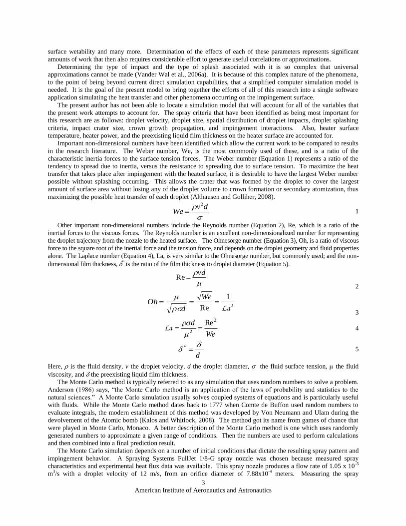
Spray cooling occurs when a liquid coolant forced through a small orifice in an atomizing spray nozzle breaks

into small droplets, as presented in Figure 1. The resulting spray droplets travel from the spray nozzle to a heated

surface. Droplet impingement on the heated surface produces a thin liquid layer on the surface. Newly impinging

droplets provide fresh cool liquid at the surface thus increasing the local heat transfer rate. However, the

complicated multiphysics occurring on the heated surface is not fully understood; therefore, extensive research on

spray cooling is ongoing.

Figure 1. Spray cooling schematic and high speed video image.

The two major efforts driving improvements in spray cooling are computational fluid dynamics (CFD) and

experimental work. Experimentation can take weeks, months, or even years to design, build and test completely;

and each change in experimental conditions might require additional implementation time. CFD iteratively solves a

representative series of equations for a defined geometry. Complicated and refined meshes corresponding to a

detailed geometry can increase the simulation time dramatically. A recent 129 x 129 x 129 grid, 3-D spray cooling

CFD simulation was solved using the preconditioned conjugate gradient solver, using the level set method, requiring

60 days to solve on a serial PC (Sarkar and Selvam, 2009). Using a multigrid conjugate gradient solver with 32

processers improved the simulation time to approximately 30 hours. It was noted that in this simulation, symmetry

conditions were used so that it represented an infinite array of equal-sized and equally-spaced droplets

simultaneously impacting the heated surface, symmetrically surrounding a second infinite array of equal-sized vapor

bubbles in the liquid film. Due to the varying conditions of spray droplet size and velocity, developing an accurate

simulation cannot be accomplished by simply combining a series of single droplet impacts (Roisman and Tropea,

2002) as others have proposed.

Therefore, a simpler model that approximates the physical behavior of spray impingement with minimal run time

constraints can yield a useful method for designing heat transfer systems using spray cooling. It has been the goal of

the present work to develop such a model. The results presented in this study show that such a simplified computer

model can be a valuable design tool. According to Selvam et al., 2006, a “theoretical understanding of the spray

cooling heat acquisition phenomena is still in its infancy and a focused effort to develop a comprehensive numerical

model is a prime importance to this field.” Development of a flexible computer model that can be adjusted

according to the latest “state of the art” results gathered from more focused experimental and CFD modeling studies

would be a tremendous asset to spray cooling researchers.

Spray cooling relies on two phase heat transfer in combination with convective liquid movement to remove heat

from the surface (Chen et al., 2004). While most spray cooling research has focused on studying how specific

enhancements affect the resulting heat transfer rate, a composite model incorporates results from each study. The

present work has developed a computer model that closely simulates the droplet impingement physics occurring

during a heated spray cooling experiment using several of the resulting correlations from these studies. A

Lagrangian-Eulerian approach has been used in the current model to follow individual droplets impinging on a

heated surface and the resulting surface behavior.

Work by Chen et al., 2004, Glaspell, 2006, Kreitzer, 2006, Puterbaugh et al., 2007, Silk et al., 2008, Vander Wal et

al., 2006a-c, and Yerkes et al., 2006 has established that there are many different physical parameters that affect and

improve the heat transfer rate during spray impingement. Some of these include but are not limited to, the droplet

velocity, droplet number flux, surface temperature, surface roughness, liquid air content, impact angle, impact type,

Nozzle

Spray

Heater

American Institute of Aeronautics and Astronautics

3

surface wetability and many more. Determination of the effects of each of these parameters represents significant

amounts of work that then also requires considerable effort to generate useful correlations or approximations.

Determining the type of impact and the type of splash associated with it is so complex that universal

approximations cannot be made (Vander Wal et al., 2006a). It is because of this complex nature of the phenomena,

to the point of being beyond current direct simulation capabilities, that a simplified computer simulation model is

needed. It is the goal of the present model to bring together the efforts of all of this research into a single software

application simulating the heat transfer and other phenomena occurring on the impingement surface.

The present author has not been able to locate a simulation model that will account for all of the variables that

the present work attempts to account for. The spray criteria that have been identified as being most important for

this research are as follows: droplet velocity, droplet size, spatial distribution of droplet impacts, droplet splashing

criteria, impact crater size, crown growth propagation, and impingement interactions. Also, heater surface

temperature, heater power, and the preexisting liquid film thickness on the heater surface are accounted for.

Important non-dimensional numbers have been identified which allow the current work to be compared to results

in the research literature. The Weber number, We, is the most commonly used of these, and is a ratio of the

characteristic inertia forces to the surface tension forces. The Weber number (Equation 1) represents a ratio of the

tendency to spread due to inertia, versus the resistance to spreading due to surface tension. To maximize the heat

transfer that takes place after impingement with the heated surface, it is desirable to have the largest Weber number

possible without splashing occurring. This allows the crater that was formed by the droplet to cover the largest

amount of surface area without losing any of the droplet volume to crown formation or secondary atomization, thus

maximizing the possible heat transfer of each droplet (Althausen and Golliher, 2008).

dvWe

2

1

Other important non-dimensional numbers include the Reynolds number (Equation 2), Re, which is a ratio of the

inertial forces to the viscous forces. The Reynolds number is an excellent non-dimensionalized number for representing

the droplet trajectory from the nozzle to the heated surface. The Ohnesorge number (Equation 3), Oh, is a ratio of viscous

force to the square root of the inertial force and the tension force, and depends on the droplet geometry and fluid properties

alone. The Laplace number (Equation 4), La, is very similar to the Ohnesorge number, but commonly used; and the non-

dimensional film thickness, * is the ratio of the film thickness to droplet diameter (Equation 5).

vdRe

2

2La

1

Re

We

dOh

3

We

d 2

2

Re

La 4

d

* 5

Here, is the fluid density, v the droplet velocity, d the droplet diameter, the fluid surface tension, the fluid

viscosity, and the preexisting liquid film thickness.

The Monte Carlo method is typically referred to as any simulation that uses random numbers to solve a problem.

Anderson (1986) says, “the Monte Carlo method is an application of the laws of probability and statistics to the

natural sciences.” A Monte Carlo simulation usually solves coupled systems of equations and is particularly useful

with fluids. While the Monte Carlo method dates back to 1777 when Comte de Buffon used random numbers to

evaluate integrals, the modern establishment of this method was developed by Von Neumann and Ulam during the

devolvement of the Atomic bomb (Kalos and Whitlock, 2008). The method got its name from games of chance that

were played in Monte Carlo, Monaco. A better description of the Monte Carlo method is one which uses randomly

generated numbers to approximate a given range of conditions. Then the numbers are used to perform calculations

and then combined into a final prediction result.

The Monte Carlo simulation depends on a number of initial conditions that dictate the resulting spray pattern and

impingement behavior. A Spraying Systems FullJet 1/8-G spray nozzle was chosen because measured spray

characteristics and experimental heat flux data was available. This spray nozzle produces a flow rate of 1.05 x 10-5

m3/s with a droplet velocity of 12 m/s, from an orifice diameter of 7.88x10

-4 meters. Measuring the spray

American Institute of Aeronautics and Astronautics

4

characteristics provided droplet diameter distribution data with a Sauter mean diameter of 48 m (spray droplet

range from 10 m to 110 m) and representative data for a radial distribution of droplet number flux.

During the impingement process a thin liquid film is generated on the heater surface prior to the liquid flowing

off the edge of the heater. A wide range of values for the film thickness have been identified, ranging from 44 to

300 m. Recent high speed video observations of impingement on a smooth flat unheated surface appeared to be on

the lower end of this range, and therefore, a film thickness of 50 m has been selected for a large portion of the

present simulation results. Cossali et al. (1997) developed a non-dimensional film thickness as the ratio of film

thickness to impinging droplet size (Equation 5). Most of the non-dimensional film thickness values of the current

model fall between values of one and three, corresponding to an intermediate film thickness.

Crater formation and secondary atomization or splashing have been the focus of numerous research studies.

Focusing on the growth of an impingement crater has produced different correlations for crater size prediction.

However, the most common value that was seen in the literature was a droplet diameter to crown radius ratio of

approximately 2.7, which is a result of combining work by Bernardin et al. (1996) and Sivakumar and Tropea

(2002). Splashing is a major concern for evaluating heat transfer on a heated surface, because it determines how

much cooling liquid is available to each location on the heated surface. Because heat transfer is driven by the

amount of fresh cool liquid that can reach the surface, the model that relies on maximum crater spreading during

impact was chosen. Vander Wal et al. (2006c) identified a splash/non-splash boundary for values of the square root

of Weber number greater than 20 resulting in a splash.

Droplet interactions play a major part in the resulting surface behavior during impingement. Since only visual

interpretations were identified for this aspect of spray cooling, an arbitrary overlap criterion has been established.

This research focuses on a few particular parameters of spray cooling; future work should include as many

additional design correlations as possible.

II. Monte Carlo Model Explanation

Successful modeling requires that a simulation be based on realistic physical conditions. This was

accomplished by basing the current simulation on results from experiments and CFD simulations. Random number

generation is the foundation of Monte Carlo Simulations. Using this technique values for droplet diameter and

location, via impact radius and angle, were generated matching experimental data for the same spraying conditions.

A more detailed explanation of the program can be found in Kreitzer (2010).

The first step in programming the simulation was to select the programming language. MATLAB was chosen

because of availability and widespread use. Also, MATLAB has user friendly graphical interfacing with tremendous

image processing capabilities. Having this interface was very important during model development, because it

provided instant feedback and showed the results graphically.

This spray cooling simulation has been broken down into four main sections or programming blocks. First

the parameter input block of the program sets the initial boundary conditions and input parameters which include

fluid properties and spray geometry. Using random numbers and subsequent calculations developed in the droplet

initialization block, the simulation attempts to mirror the complex nature of spray cooling. Identifying what happens

once the droplet hits the heater surface occurs in the crater formation and tracking block of the program. Finally, the

movement and display block scans the heater surface, tracking crater movement and calculating heater surface heat

transfer regimes. An in depth description of each of the four programming blocks can be found in Kreitzer (2010).

A. Monte Carlo Random Number Generation

Harris (2009) at the Air Force Research Laboratory has used PDA techniques to study the resulting behavior and

trends of this particular spray nozzle. Using a bin wise representation of Harris‟s measured data provides

probability density functions for both the droplet diameter distribution and the radial flux distribution. Experimental

conditions of the PDA analysis were set such that the spray would cover a heated surface that had been mounted on

a 16 mm diameter pedestal. This setup created a spacing between the spray nozzle and heater surface of 13 mm.

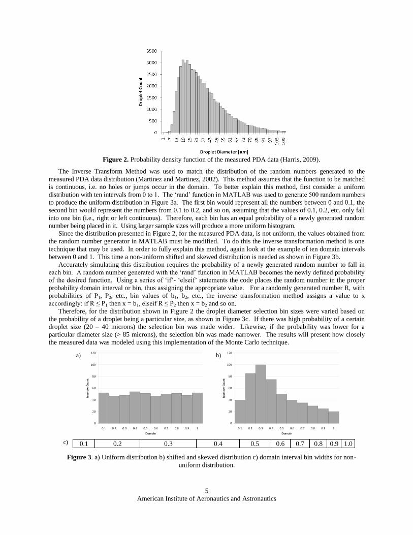
Diameter distribution data was collected with a bin resolution of 2 microns. Figure 2 represents the collected PDA

data (Harris, 2009), tracking 60,000 drops. In order to accurately simulate this data a bin wise method tracked the

number of droplets in each selection bin and calculated the probability of new droplets falling in each bin.

American Institute of Aeronautics and Astronautics

5

Figure 2. Probability density function of the measured PDA data (Harris, 2009).

The Inverse Transform Method was used to match the distribution of the random numbers generated to the

measured PDA data distribution (Martinez and Martinez, 2002). This method assumes that the function to be matched

is continuous, i.e. no holes or jumps occur in the domain. To better explain this method, first consider a uniform

distribution with ten intervals from 0 to 1. The „rand‟ function in MATLAB was used to generate 500 random numbers

to produce the uniform distribution in Figure 3a. The first bin would represent all the numbers between 0 and 0.1, the

second bin would represent the numbers from 0.1 to 0.2, and so on, assuming that the values of 0.1, 0.2, etc. only fall

into one bin (i.e., right or left continuous). Therefore, each bin has an equal probability of a newly generated random

number being placed in it. Using larger sample sizes will produce a more uniform histogram.

Since the distribution presented in Figure 2, for the measured PDA data, is not uniform, the values obtained from

the random number generator in MATLAB must be modified. To do this the inverse transformation method is one

technique that may be used. In order to fully explain this method, again look at the example of ten domain intervals

between 0 and 1. This time a non-uniform shifted and skewed distribution is needed as shown in Figure 3b.

Accurately simulating this distribution requires the probability of a newly generated random number to fall in

each bin. A random number generated with the „rand‟ function in MATLAB becomes the newly defined probability

of the desired function. Using a series of „if‟- „elseif‟ statements the code places the random number in the proper

probability domain interval or bin, thus assigning the appropriate value. For a randomly generated number R, with

probabilities of P1, P2, etc., bin values of b1, b2, etc., the inverse transformation method assigns a value to x

accordingly: if R ≤ P1 then x = b1, elseif R ≤ P2 then x = b2 and so on.

Therefore, for the distribution shown in Figure 2 the droplet diameter selection bin sizes were varied based on

the probability of a droplet being a particular size, as shown in Figure 3c. If there was high probability of a certain

droplet size (20 – 40 microns) the selection bin was made wider. Likewise, if the probability was lower for a

particular diameter size (> 85 microns), the selection bin was made narrower. The results will present how closely

the measured data was modeled using this implementation of the Monte Carlo technique.

Figure 3. a) Uniform distribution b) shifted and skewed distribution c) domain interval bin widths for non-

uniform distribution.

a) b)

0.1 0.2 0.3 0.4 0.5 0.6 0.7 0.8 0.9 1.0 c)

American Institute of Aeronautics and Astronautics

6

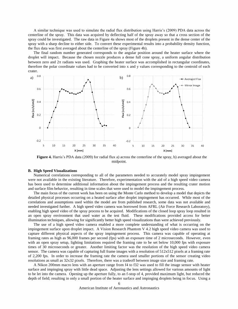
A similar technique was used to simulate the radial flux distribution using Harris‟s (2009) PDA data across the

centerline of the spray. This data was acquired by deflecting half of the spray away so that a cross section of the

spray could be investigated. The raw data in Figure 4a shows most of the droplets present in the dense center of the

spray with a sharp decline to either side. To convert these experimental results into a probability density function,

the flux data was first averaged about the centerline of the spray (Figure 4b).

The final random number generated corresponds to the angular position around the heater surface where the

droplet will impact. Because the chosen nozzle produces a dense full cone spray, a uniform angular distribution

between zero and 2 radians was used. Graphing the heater surface was accomplished in rectangular coordinates,

therefore the polar coordinate values had to be converted into x and y values corresponding to the centroid of each

crater.

Figure 4. Harris‟s PDA data (2009) for radial flux a) across the centerline of the spray, b) averaged about the

midpoint.

B. High Speed Visualizations

Numerical correlations corresponding to all of the parameters needed to accurately model spray impingement

were not available in the existing literature. Therefore, experimentation with the aid of a high speed video camera

has been used to determine additional information about the impingement process and the resulting crater motion

and surface film behavior, resulting in time scales that were used to model the impingement process.

The main focus of the current work has been on using the Monte Carlo method to develop a model that depicts the

detailed physical processes occurring on a heated surface after droplet impingement has occurred. While most of the

correlations and assumptions used within the model are from published research, some data was not available and

needed investigated further. A high speed video camera was borrowed from AFRL (Air Force Research Laboratory),

enabling high speed video of the spray process to be acquired. Modifications of the closed loop spray loop resulted in

an open spray environment that used water as the test fluid. These modifications provided access for better

illumination techniques, allowing for significantly better high speed visualizations than were achieved previously.

The use of a high speed video camera enabled a more complete understanding of what is occurring on the

impingement surface upon droplet impact. A Vision Research Phantom V 4.2 high speed video camera was used to

capture different physical aspects of the spray impingement process. This camera was capable of operating at

framing rates as high as 96,000 frames per second (fps) with an exposure time of 2 microseconds. However, even

with an open spray setup, lighting limitations required the framing rate to be set below 10,000 fps with exposure

times of 30 microseconds or greater. Another limiting factor was the resolution of the high speed video camera

sensor. The camera was capable of capturing full frame images with a resolution of 512x512 pixels at a framing rate

of 2,200 fps. In order to increase the framing rate the camera used smaller portions of the sensor creating video

resolutions as small as 32x32 pixels. Therefore, there was a tradeoff between image size and framing rate.

A Nikon 200mm macro lens with an aperture range from f4 to f32 was used to fill the image sensor with heater

surface and impinging spray with little dead space. Adjusting the lens settings allowed for various amounts of light

to be let into the camera. Opening up the aperture fully, to an f-stop of 4, provided maximum light, but reduced the

depth of field; resulting in only a small portion of the heater surface and impinging droplets being in focus. Using a

a) b)

American Institute of Aeronautics and Astronautics

7

wide open aperture expanded the allowable framing rate to as high as 25,000 fps. Conversely, setting the lens to an

f-stop of 32 provided a very large depth of field, but restricted the framing rate to no faster than 2,500 fps with a

relatively high exposure time.

The spray impingement surface was an unheated 1.25 inch diameter transparent quartz disc. Using a larger sized

spray surface required a larger spacing, of 1.125 inches, from the nozzle to the surface. This adjustment revealed

that the spray was not fully atomized for the prior experimental setup which used a 13 mm nozzle-to-heater spacing

for the heat transfer studies. A rotometer and pressure gauge were installed between the water reservoir and the

spray nozzle to record spray conditions.

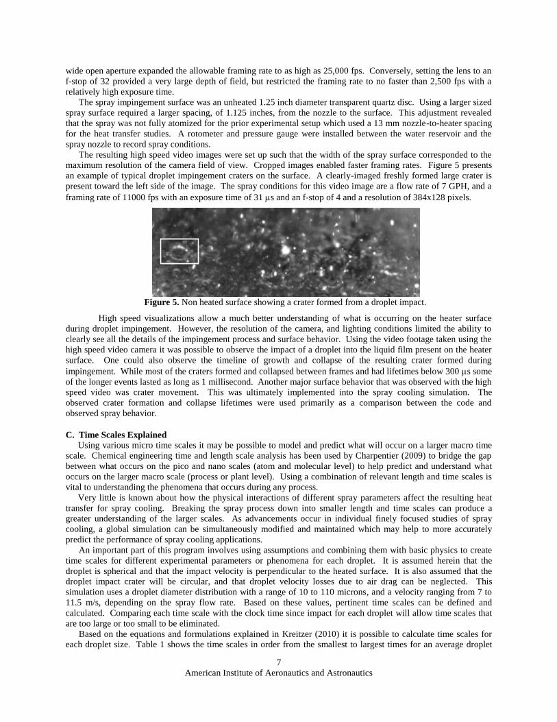
The resulting high speed video images were set up such that the width of the spray surface corresponded to the

maximum resolution of the camera field of view. Cropped images enabled faster framing rates. Figure 5 presents

an example of typical droplet impingement craters on the surface. A clearly-imaged freshly formed large crater is

present toward the left side of the image. The spray conditions for this video image are a flow rate of 7 GPH, and a

framing rate of 11000 fps with an exposure time of 31 s and an f-stop of 4 and a resolution of 384x128 pixels.

Figure 5. Non heated surface showing a crater formed from a droplet impact.

High speed visualizations allow a much better understanding of what is occurring on the heater surface

during droplet impingement. However, the resolution of the camera, and lighting conditions limited the ability to

clearly see all the details of the impingement process and surface behavior. Using the video footage taken using the

high speed video camera it was possible to observe the impact of a droplet into the liquid film present on the heater

surface. One could also observe the timeline of growth and collapse of the resulting crater formed during

impingement. While most of the craters formed and collapsed between frames and had lifetimes below 300 s some

of the longer events lasted as long as 1 millisecond. Another major surface behavior that was observed with the high

speed video was crater movement. This was ultimately implemented into the spray cooling simulation. The

observed crater formation and collapse lifetimes were used primarily as a comparison between the code and

observed spray behavior.

C. Time Scales Explained

Using various micro time scales it may be possible to model and predict what will occur on a larger macro time

scale. Chemical engineering time and length scale analysis has been used by Charpentier (2009) to bridge the gap

between what occurs on the pico and nano scales (atom and molecular level) to help predict and understand what

occurs on the larger macro scale (process or plant level). Using a combination of relevant length and time scales is

vital to understanding the phenomena that occurs during any process.

Very little is known about how the physical interactions of different spray parameters affect the resulting heat

transfer for spray cooling. Breaking the spray process down into smaller length and time scales can produce a

greater understanding of the larger scales. As advancements occur in individual finely focused studies of spray

cooling, a global simulation can be simultaneously modified and maintained which may help to more accurately

predict the performance of spray cooling applications.

An important part of this program involves using assumptions and combining them with basic physics to create

time scales for different experimental parameters or phenomena for each droplet. It is assumed herein that the

droplet is spherical and that the impact velocity is perpendicular to the heated surface. It is also assumed that the

droplet impact crater will be circular, and that droplet velocity losses due to air drag can be neglected. This

simulation uses a droplet diameter distribution with a range of 10 to 110 microns, and a velocity ranging from 7 to

11.5 m/s, depending on the spray flow rate. Based on these values, pertinent time scales can be defined and

calculated. Comparing each time scale with the clock time since impact for each droplet will allow time scales that

are too large or too small to be eliminated.

Based on the equations and formulations explained in Kreitzer (2010) it is possible to calculate time scales for

each droplet size. Table 1 shows the time scales in order from the smallest to largest times for an average droplet

American Institute of Aeronautics and Astronautics

8

occurring at the Sauter mean diameter of 48 m for three different time scales. The first is the dimensional time in

microseconds, the second is non-dimensionalized with respect to the time for the droplet to move a distance equal to

the liquid film thickness, and the third is number of simulation intervals (time between simulation droplet impacts).

These values are based on a flowrate of 10 GPH with a droplet velocity of 12 m/s and a heater power of 100 W. The

time between droplet impacts is on the shortest order, while the time for waves to fill a crater back in are on the

largest order, and thus rarely occur.

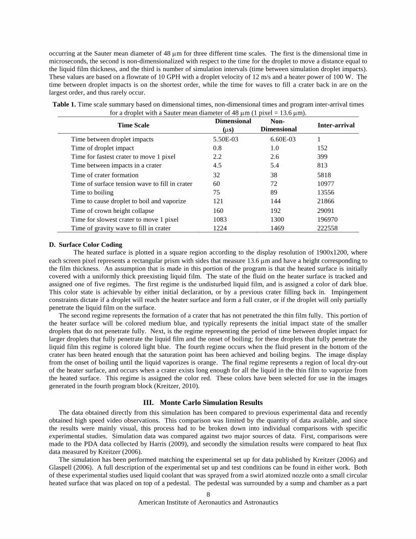
Table 1. Time scale summary based on dimensional times, non-dimensional times and program inter-arrival times

for a droplet with a Sauter mean diameter of 48 m (1 pixel = 13.6 m).

Time Scale Dimensional

(s)

Non-

Dimensional Inter-arrival

Time between droplet impacts 5.50E-03 6.60E-03 1

Time of droplet impact 0.8 1.0 152

Time for fastest crater to move 1 pixel 2.2 2.6 399

Time between impacts in a crater 4.5 5.4 813

Time of crater formation 32 38 5818

Time of surface tension wave to fill in crater 60 72 10977

Time to boiling 75 89 13556

Time to cause droplet to boil and vaporize 121 144 21866

Time of crown height collapse 160 192 29091

Time for slowest crater to move 1 pixel 1083 1300 196970

Time of gravity wave to fill in crater 1224 1469 222558

D. Surface Color Coding

The heated surface is plotted in a square region according to the display resolution of 1900x1200, where

each screen pixel represents a rectangular prism with sides that measure 13.6 m and have a height corresponding to

the film thickness. An assumption that is made in this portion of the program is that the heated surface is initially

covered with a uniformly thick preexisting liquid film. The state of the fluid on the heater surface is tracked and

assigned one of five regimes. The first regime is the undisturbed liquid film, and is assigned a color of dark blue.

This color state is achievable by either initial declaration, or by a previous crater filling back in. Impingement

constraints dictate if a droplet will reach the heater surface and form a full crater, or if the droplet will only partially

penetrate the liquid film on the surface.

The second regime represents the formation of a crater that has not penetrated the thin film fully. This portion of

the heater surface will be colored medium blue, and typically represents the initial impact state of the smaller

droplets that do not penetrate fully. Next, is the regime representing the period of time between droplet impact for

larger droplets that fully penetrate the liquid film and the onset of boiling; for these droplets that fully penetrate the

liquid film this regime is colored light blue. The fourth regime occurs when the fluid present in the bottom of the

crater has been heated enough that the saturation point has been achieved and boiling begins. The image display

from the onset of boiling until the liquid vaporizes is orange. The final regime represents a region of local dry-out

of the heater surface, and occurs when a crater exists long enough for all the liquid in the thin film to vaporize from

the heated surface. This regime is assigned the color red. These colors have been selected for use in the images

generated in the fourth program block (Kreitzer, 2010).

III. Monte Carlo Simulation Results

The data obtained directly from this simulation has been compared to previous experimental data and recently

obtained high speed video observations. This comparison was limited by the quantity of data available, and since

the results were mainly visual, this process had to be broken down into individual comparisons with specific

experimental studies. Simulation data was compared against two major sources of data. First, comparisons were

made to the PDA data collected by Harris (2009), and secondly the simulation results were compared to heat flux

data measured by Kreitzer (2006).

The simulation has been performed matching the experimental set up for data published by Kreitzer (2006) and

Glaspell (2006). A full description of the experimental set up and test conditions can be found in either work. Both

of these experimental studies used liquid coolant that was sprayed from a swirl atomized nozzle onto a small circular

heated surface that was placed on top of a pedestal. The pedestal was surrounded by a sump and chamber as a part

American Institute of Aeronautics and Astronautics

9

of a closed loop fluid management system. The pedestal heater had a diameter of 16 mm, an active heating area of

1.46 cm2, with a 13 mm distance between the nozzle and the heated surface.

Fluid properties were defined for a spray temperature of 25 C, with nine degrees sub-cooling. PDA measurements

taken by Harris (2009) showed a droplet distribution between 10 and 110 m with a Sauter mean diameter of 48 m at

a flow rate of 10 GPH. Another initial condition that was used was the fluid volume in the initial liquid film present on

the heater surface. The liquid film has been assumed to have a uniform thickness of 50 m. This value falls within the

published values of Selvam et al. (2006), Pautsch et al. (2004), and Kreitzer and Kuhlman (2008).

Parametric variations of the simulation show how changing the various parameters affect the model performance

prediction. The most important parameter that needed to be studied was how the liquid film reacted to various

heater power settings. Using a constant heat flux across the heater surface allowed for the simulation to reach steady

state in a predictable manner. Varying the heater power from 60 W to 160 W ensured that the comparable

experimental results were bracketed.

A. Droplet Diameter and Radial Flux Distribution

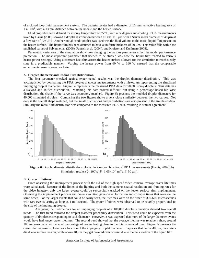
The first parameter checked against experimental results was the droplet diameter distribution. This was

accomplished by comparing the PDA droplet diameter measurements with a histogram representing the simulated

impinging droplet diameters. Figure 6a represents the measured PDA data for 58,000 spray droplets. This data has

a skewed and shifted distribution. Matching this data proved difficult, but using a percentage based bin wise

distribution, the shape of the curve was accurately matched. Figure 6b presents the modeled droplet diameters for

40,000 simulated droplets. Comparing the two figures shows a very close similarity between the two curves. Not

only is the overall shape matched, but the small fluctuations and perturbations are also present in the simulated data.

Similarly the radial flux distribution was compared to the measured PDA data, resulting in similar agreement.

Figure 6. Droplet diameter distributions plotted in 2 micron bins for: a) PDA measurements (Harris, 2009), b)

Simulation results (𝑄 =100W, 𝑉 =1.05x10-5

m3/s, =50 m).

B. Crater Lifetimes

From observing the impingement process with the aid of the high speed video camera, average crater lifetimes

were calculated. Because of the limits of the lighting and both the cameras spatial resolution and framing rates for

the video imagery, only the larger events could be successfully tracked on the heater surface after impingement.

Observing the impingement process and crater evolution gave crater formation and collapse times that were on the

same order. For the larger events that could be easily seen, the lifetimes were on the order of 300-600 microseconds

with rare events lasting as long as 1 millisecond. The crater lifetimes were observed to be roughly proportional to

the size of the impinging droplet.

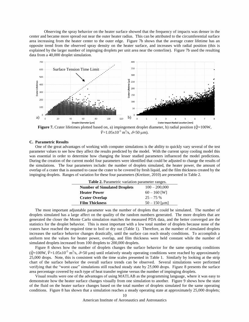
Analyzing the lifetime data for all impinging droplets of a 100,000 droplet simulation showed two overall

trends. The first trend mirrored the droplet diameter probability distribution. This trend could be expected from the

quantity of droplets corresponding to each diameter. However, it was expected that more of the larger diameter events

would have had longer crater lifetimes. The second trend showed that the average lifetime was relatively short, around

100 microseconds, with a small percentage of craters lasting close to the total simulated time. Figure 7a presents the

crater lifetime results plotted as a function of the impinging droplet diameter. It appears that below 40 m, the craters

die due to surface tension, while above 40 m they get covered over or reset due to the bulk motion of the liquid film.

a) b)

American Institute of Aeronautics and Astronautics

10

Observing the spray behavior on the heater surface showed that the frequency of impacts was denser in the

center and became more spread out near the outer heater radius. This can be attributed to the circumferential surface

area increasing from the heater center to the outer edge. Figure 7b shows that the average crater lifetime has an

opposite trend from the observed spray density on the heater surface, and increases with radial position (this is

explained by the larger number of impinging droplets per unit area near the centerline). Figure 7b used the resulting

data from a 40,000 droplet simulation.

Figure 7. Crater lifetimes plotted based on, a) impingement droplet diameter, b) radial position (𝑄 =100W,

𝑉 =1.05x10-5

m3/s, =50 m).

C. Parametric Results

One of the great advantages of working with computer simulations is the ability to quickly vary several of the test

parameter values to see how they affect the results predicted by the model. With the current spray cooling model this

was essential in order to determine how changing the lesser studied parameters influenced the model predictions.

During the creation of the current model four parameters were identified that could be adjusted to change the results of

the simulations. The four parameters include: the number of droplets simulated, the heater power, the amount of

overlap of a crater that is assumed to cause the crater to be covered by fresh liquid, and the film thickness created by the

impinging droplets. Ranges of variation for these four parameters (Kreitzer, 2010) are presented in Table 2.

Table 2. Parametric variation parameter ranges.

Number of Simulated Droplets 100 – 200,000

Heater Power 60 – 160 [W]

Crater Overlap 25 – 75 %

Film Thickness 50 – 150 [m]

The most important adjustable parameter was the number of droplets that could be simulated. The number of

droplets simulated has a large affect on the quality of the random numbers generated. The more droplets that are

generated the closer the Monte Carlo simulation matches the measured PDA data, and the better converged are the

statistics for the droplet behavior. This is most important with a low total number of droplets because none of the

craters have reached the required time to boil or dry out (Table 1). Therefore, as the number of simulated droplets

increases the surface behavior changes drastically, until the surface can reach steady conditions. To accomplish a

uniform test the values for heater power, overlap, and film thickness were held constant while the number of

simulated droplets increased from 100 droplets to 200,000 droplets.

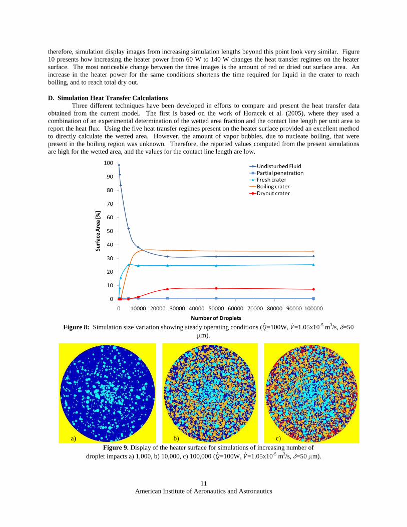
Figure 8 shows how the number of droplets changes the surface behavior for the same operating conditions

(𝑄 =100W, 𝑉 =1.05x10-5

m3/s, =50 m) until relatively steady operating conditions were reached by approximately

25,000 drops. Note, this is consistent with the time scales presented in Table 1. Similarly by looking at the strip

chart of the surface behavior the overall surface trends can be observed. Several simulations were performed

verifying that the “worst case” simulations still reached steady state by 25,000 drops. Figure 8 presents the surface

area percentage covered by each type of heat transfer regime versus the number of impinging droplets.

Visual results were one of the advantages of using MATLAB as the programming language, where it was easy to

demonstrate how the heater surface changes visually from one simulation to another. Figure 9 shows how the state

of the fluid on the heater surface changes based on the total number of droplets simulated for the same operating

conditions. Figure 8 has shown that a simulation reaches a steady operating state at approximately 25,000 droplets;

Surface Tension Time Limit

a) b)

American Institute of Aeronautics and Astronautics

11

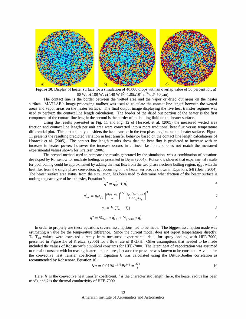
therefore, simulation display images from increasing simulation lengths beyond this point look very similar. Figure

10 presents how increasing the heater power from 60 W to 140 W changes the heat transfer regimes on the heater

surface. The most noticeable change between the three images is the amount of red or dried out surface area. An

increase in the heater power for the same conditions shortens the time required for liquid in the crater to reach

boiling, and to reach total dry out.

D. Simulation Heat Transfer Calculations

Three different techniques have been developed in efforts to compare and present the heat transfer data

obtained from the current model. The first is based on the work of Horacek et al. (2005), where they used a

combination of an experimental determination of the wetted area fraction and the contact line length per unit area to

report the heat flux. Using the five heat transfer regimes present on the heater surface provided an excellent method

to directly calculate the wetted area. However, the amount of vapor bubbles, due to nucleate boiling, that were

present in the boiling region was unknown. Therefore, the reported values computed from the present simulations

are high for the wetted area, and the values for the contact line length are low.

Figure 8: Simulation size variation showing steady operating conditions (𝑄 =100W, 𝑉 =1.05x10

-5 m

3/s, =50

m).

Figure 9. Display of the heater surface for simulations of increasing number of

droplet impacts a) 1,000, b) 10,000, c) 100,000 (𝑄 =100W, 𝑉 =1.05x10-5

m3/s, =50 m).

a) b) c)

American Institute of Aeronautics and Astronautics

12

Figure 10. Display of heater surface for a simulation of 40,000 drops with an overlap value of 50 percent for: a)

60 W, b) 100 W, c) 140 W (𝑉 =1.05x10-5

m3/s, =50 m).

The contact line is the border between the wetted area and the vapor or dried out areas on the heater

surface. MATLAB‟s image processing toolbox was used to calculate the contact line length between the wetted

areas and vapor areas on the heater surface. The final output image displaying the five heat transfer regimes was

used to perform the contact line length calculation. The border of the dried out portion of the heater is the first

component of the contact line length; the second is the border of the boiling fluid on the heater surface.

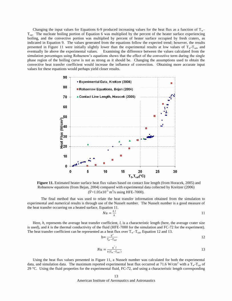
Using the results presented in Fig. 11 and Fig. 12 of Horacek et al. (2005) the measured wetted area

fraction and contact line length per unit area were converted into a more traditional heat flux versus temperature

differential plot. This method only considers the heat transfer in the two phase regions on the heater surface. Figure

11 presents the resulting predicted variation in heat transfer behavior based on the contact line length calculations of

Horacek et al. (2005). The contact line length results show that the heat flux is predicted to increase with an

increase in heater power; however the increase occurs in a linear fashion and does not match the measured

experimental values shown for Kreitzer (2006).

The second method used to compare the results generated by the simulation, was a combination of equations

developed by Rohsenow for nucleate boiling, as presented in Bejan (2004). Rohsenow showed that experimental results

for pool boiling could be approximated by adding the heat flux from the two phase nucleate boiling region, 𝑞𝑛𝑏" , with the

heat flux from the single phase convection, 𝑞𝑐" , occurring on the heater surface, as shown in Equations 6-8 (Bejan, 2004).

The heater surface area status, from the simulation, has been used to determine what fraction of the heater surface is

undergoing each type of heat transfer, Equation 9.

𝑞" = 𝑞𝑛𝑏" + 𝑞𝑐

" 6

𝑞𝑛𝑏" = 𝜇𝑙𝑕𝑓𝑔

𝑔 𝜌𝑙−𝜌𝑣

𝜎

1/2

𝑐𝑝 ,𝑙 𝑇𝑤−𝑇𝑠𝑎𝑡

𝑃𝑟𝑙𝑠𝐶𝑠𝑓𝑕𝑓𝑔

3

7

𝑞𝑐" = 𝑕𝑐 𝑇𝑤 − 𝑇𝑙 8

𝑞" = %𝑏𝑜𝑖𝑙 ∗ 𝑞𝑛𝑏" + %𝑓𝑟𝑒𝑠𝑕 ∗ 𝑞𝑐

" 9

In order to properly use these equations several assumptions had to be made. The biggest assumption made was

estimating a value for the temperature difference. Since the current model does not report temperatures directly,

Tw–Tsat values were extracted directly from measured experimental data, for spray cooling with HFE-7000,

presented in Figure 5.6 of Kreitzer (2006) for a flow rate of 8 GPH. Other assumptions that needed to be made

included the values of Rohsneow‟s empirical constants for HFE-7000. The latent heat of vaporization was assumed

to remain constant with increasing heater temperatures, because the pressure was known to be constant. A value for

the convective heat transfer coefficient in Equation 8 was calculated using the Dittus-Boelter correlation as

recommended by Rohsenow, Equation 10.

𝑁𝑢 = 0.019𝑅𝑒4/5𝑃𝑟0.4 =𝑕𝑐 𝑙

𝑘 10

Here, hc is the convective heat transfer coefficient, l is the characteristic length (here, the heater radius has been

used), and k is the thermal conductivity of HFE-7000.

a) b) c)

American Institute of Aeronautics and Astronautics

13

Changing the input values for Equations 6-9 produced increasing values for the heat flux as a function of Tw–

Tsat. The nucleate boiling portion of Equation 6 was multiplied by the percent of the heater surface experiencing

boiling, and the convective portion was multiplied by percent of heater surface occupied by fresh craters, as

indicated in Equation 9. The values generated from the equations follow the expected trend; however, the results

presented in Figure 11 were initially slightly lower than the experimental results at low values of Tw-Tsat, and

eventually lie above the experimental values. Examining the difference between the values calculated from the

simulation percentages using Rohsenow‟s equations shows that the effect of the convective term during the single

phase region of the boiling curve is not as strong as it should be. Changing the assumptions used to obtain the

convective heat transfer coefficient would increase the influence of convection. Obtaining more accurate input

values for these equations would perhaps yield closer results.

Figure 11. Estimated heater surface heat flux values based on contact line length (from Horacek, 2005) and

Rohsenow equations (from Bejan, 2004) compared with experimental data collected by Kreitzer (2006)

(𝑉 =1.05x10-5

m3/s using HFE-7000).

The final method that was used to relate the heat transfer information obtained from the simulation to

experimental and numerical results is through use of the Nusselt number. The Nusselt number is a good measure of

the heat transfer occurring on a heated surface, Equation 11.

𝑁𝑢 =𝑕 𝑙

𝑘 11

Here, h, represents the average heat transfer coefficient, l, is a characteristic length (here, the average crater size

is used), and k is the thermal conductivity of the fluid (HFE-7000 for the simulation and FC-72 for the experiment).

The heat transfer coefficient can be represented as a heat flux over Tw–Tsat, Equation 12 and 13.

h=𝑞"

𝑇𝑤−𝑇𝑠𝑎𝑡 12

𝑁𝑢 =𝑞" 𝑙

𝑘 𝑇𝑤−𝑇𝑠𝑎𝑡 13

Using the heat flux values presented in Figure 11, a Nusselt number was calculated for both the experimental

data, and simulation data. The maximum reported experimental heat flux occurred at 71.6 W/cm2 with a Tw-Tsat of

29 °C. Using the fluid properties for the experimental fluid, FC-72, and using a characteristic length corresponding

American Institute of Aeronautics and Astronautics

14

to the average crater radius (48 m droplet Sauter mean diameter * 2.67) produced a Nusselt number of 55.5. The

measured heat flux over the experimental surface area of 1.46 cm2, an applied heat level of 110 W was used. Using

the simulation results with the Rohsenow equations for an applied heat load of 100 W resulted in a heat flux of 22

W/cm2 with a Tw-Tsat of 16.9 °C. Using the same characteristic length and the simulation fluid properties for HFE-

7000, a comparable Nusselt number of 22.3 was calculated.

IV. Discussion and Conclusions

Spray cooling droplet impingement and the resulting surface film behavior was modeled successfully using the Monte

Carlo method. Numerous design iterations took the simulation from an initial concept and has produced a final working

model of spray impingement on a heated surface using correlations from the literature, along with calculated physical time

scales. This was accomplished by matching randomly generated numbers with probability density functions

corresponding to measured droplet diameter and radial flux spray data approximating a Spraying Systems 1/8-G FullJet

spray nozzle at a flow rate of 10 GPH. Droplet impingement on the heated surface resulted in crater formation on the

heated surface that could be followed from impact to vaporization and dryout utilizing time scales. The current model is

capable of simulating hundreds of thousands of droplet impacts representing a few milliseconds of the actual heat transfer

process in a few hours of computational time using a current generation quad core PC.

Comparing non-dimensional groupings with values previously published in the literature shows consistency.

The chosen simulation flow rate produces droplets with a velocity of 10 m/s and an average diameter of 48 m,

resulting in Weber numbers with a range of 300-1350, Reynolds numbers with a range of 750-3500, and Ohnesorge

numbers with a range of 0.01-0.025. Simulation results show dramatic increases in heater surface dry out when the

heater power is increased. This dryout is more pronounced near the outer edge of the heater surface, consistent with

experimental observations.

The current simulation is an ever changing representation of the current state of the art in spray cooling research.

Several basic impingement parameters were identified during a literature review. The first parameter set was the

data necessary to form the Monte Carlo spray droplet generation. Harris (2009) used a PDA to measure the droplet

diameter distribution and radial number flux for the chosen spray nozzle. The next parameter investigated

determined the number of droplet impacts resulting in a splash. Vander Wal et al. (2006c) developed a splash/non-

splash boundary; where droplets with a square root of We greater than 20 create a splash. Another important

parameter checked was impinging droplet penetration depth. This value determined if the droplet would penetrate

the liquid film completely, thus forming a full crater. For all parameters tested more than 90 percent of the droplets

penetrated the liquid film on the heater surface and formed a complete crater. Finally, a relationship was identified

that related the size of a spray droplet to the resulting crater size, where, crater radius was determined to be 2.67

times the size of the impinging droplet diameter (Sivakumar and Tropea, 2002).

Simulation heat flux values were compared to experimental values using three techniques. The first used a contact

line length in an effort to reproduce a standard heat flux T plot. The resulting curve followed the proper trend,

however, showed no non-linear behavior due to the onset of two phase heat transfer. This discrepancy was due to the

lack of a needed correlation or direct measurement of the amount of nucleation sites in the boiling regions of the heater

surface. The second method used equations developed by Rohsenow for heat transfer in flow boiling. These equations

combined the heat flux due to nucleate boiling with the heat flux generated by single-phase convection. Using the

resulting surface area percentages generated by the present simulation, a heat flux curve was generated that was in

reasonable agreement with the experimental data. Finally, using the heat flux values calculated by these equations

produced a Nu of 22.3, while values read from the experimental data produced a Nu of 55.5.

Acknowledgments

The authors would like to thank the Department of Mechanical and Aerospace Engineering at West Virginia

University, the West Virginia Space Grant Consortium, and the Office of Graduate Education and Life for partial

funding of this research.

References

Althausen, D.M., and Golliher, E.L., “Testing of an R134a Spray Evaporative Heat Sink,” SAE International Conference on

Environmental Systems, San Francisco, CA, 2008-01-2165, 2008.

Anderson, H.L., “Metropolis, Monte Carlo, and the Maniac,” Los Alamos Science, no. 14, pp. 96-108, 1986.

Bejan, A., “Convection Heat Transfer,” John Wiley & Sons, Inc., New Jersey, 2004.

American Institute of Aeronautics and Astronautics

15

Bernardin, J. D., Stebbins, C. J., and Mudawar, I., “Mapping of Impact and Heat Transfer Regimes of Water Drops

Impinging on a Polished Surface,” Int. J. Heat Mass Transfer, Vol. 40, pp. 247-267, 1996.

Charpentier, J.C., “Among the Trends for a Modern Chemical Engineering: the Time and Length Multiscale

Approach as an Efficient Tool for Process Intensification and Product Design and Engineering,”

Proceedings of WCCE8, Montreal, CA, 2009.

Chen, R., Chow, L.C., and Navedo, J.E., “Optimal Spray Characteristics in Water Spray Cooling,” International

Journal of Heat and Mass Transfer, Vol. 47, pp. 5095-5099, 2004.

Cossali, G.E., Coghe, A., Marengo, M., “The Impact of a Single Drop on a Wetted Solid Surface,” Experiments in

Fluids, Vol. 12, pp. 463-472, 1997.

Glaspell, S.L., “Effects of the Electric Kelvin Force on Spray Cooling Performance,” M.S. Thesis, West Virginia

University, Morgantown, WV, 2006.

Harris, R., Personal Communication, March, 2009.

Horacek, B., Kim, J., and Kiger, K.T., “Single Nozzle Spray Cooling Heat Transfer Mechanisms,” International Journal of Heat

and Mass Transfer, Vol. 48, pp. 1425-1438, 2005.

Kalos, M.H., and Whitlock, P.A., “Monte Carlo Methods,” Wiley-VCH Verlag GmbH & Co., Germany, 2008.

Kreitzer, P.J., “Experimental Testing of Convective Spray Cooling with the Aid of an Electrical Field Using the Coulomb

Force,” M. S. Thesis, West Virginia University, Morgantown, WV, 2006.

Kreitzer, P.J., and Kuhlman, J.M., “Visualization of Electrohydrodynamic Effects and Time Scale Analysis for

Impinging Spray Droplets of HFE-7000,” STAIF 12th

Conference on Thermophysics Applications in

Microgravity, edited by M. El-Genk, AIP Conference Proceedings, pp. 86-93, 2008.

Kreitzer, P.J., “Spray Cooling Simulation Implementing Time Scale Analysis and the Monte Carlo Method,” Ph.D

Dissertation, West Virginia University, Morgantown, WV, 2010.

Martinez, W.L., and Martinez, A.R., “ Computational Statistics Handbook with MATLAB,” Washington, D.C.,

Chapman & Hall/CRC, 2002.

Pautsch, A.G., Shedd, T.A., and Nellis, G.F., “ Thickness Measurements of the Thin Film in Spray Evaporative Cooling,”

Inter Society Conference on Thermal Phenomena, pp. 70-76, 2004.

Puterbaugh, R.L., Yerkes, K.L., Michalak, T.E., and Thomas, S.K., “Cooling Performance of a Partially-Confined FC-

72 Spray: The Effect of Dissolved Air,” 45th AIAA Aerospace Sciences Meeting and Exhibit, edited and

published by AIAA, 2007-199, Reno, NV, 2007.

Roisman, I.V., and Tropea, C., “Impact of a Drop onto a Wetted Wall: Description of Crown Formation and

Propagation,” Journal of Fluid Mechanics, Vol. 472, pp. 373-397, 2002.

Sarkar, S., and Selvam, R.P., “Direct Numerical Simulation of Heat Transfer in Spray Cooling Through 3D Multiphase

Flow Modeling Using Parallel Computing,” Journal of Heat Transfer, Vol. 131, 2009.

Selvam, R.P., Lin, L., and Ponnappan, R., “Direct Simulation of Spray Cooling: Effect of Vapor Bubble Growth and

Liquid Droplet Impact on Heat Transfer,” International Journal of Heat and Mass Transfer, Vol. 49, pp.

4265-4278, 2006.

Silk, E.A., Golliher, E.L., and Selvam, R.P., “Spray Cooling Heat Transfer: Technology Overview and Assessment

of Future Challenges for Micro-gravity Application,” Energy Conversion and Management, Vol. 49, pp.

453-468, 2008.

Sivakumar, D., and Tropea, C., “Splashing Impact of a Spray onto a Liquid Film,” Physics of Fluids, Vol. 14, No.

12, pp. L85-L88, 2002.

Vander Wal, R.L., Berger, G.M., and Mozes, S.D., “The Combined Influence of a Rough Surface and Thin Fluid

Film Upon the Splashing Threshold and Splash Dynamics of a Droplet Impacting onto Them,” Experiments

in Fluids, Vol. 40, pp. 23-32, 2006a.

Vander Wal, R.L., Berger, G.M., and Mozes, S.D., “Droplets Splashing upon Films of the Same Fluid of Various

Depths,” Experiments in Fluids, Vol. 40, pp. 33-52, 2006b.

Vander Wal, R.L., Berger, G.M., and Mozes, S.D., “The Splash/non-splash Boundary upon a Dry Surface and Thin

Fluid Film,” Experiments in Fluids, Vol. 40, pp. 53-59, 2006c.

Yang, J., Chow, L.C., and Pais, M.R., “Nucleate Boiling Heat Transfer in Spray Cooling,” Journal of Heat Transfer,

Vol. 118, pp. 668-671, 1996.

Yerkes, K.L., Michalak, T., Baysinger, K., Puterbaugh, R., Thomas, S.K., and McQuillen, J., 2006, "Variable-Gravity Effects on a

Single-Phase Partially-Confined Spray Cooling System," 44th AIAA Aerospace Sciences Meeting and Exhibit, AIAA-

2006-0596, Reno NV, 9-12 Jan. 2006.