Spousal Joint Retirement: A reform based approach to identifying spillover effects Francois Gerard,...

Spousal Joint Retirement: A reform based approach to identifying spillover effects

Francois Gerard, Department of Economics, UC Berkeley

and

Lena Nekby, Department of Economics, Stockholm University

and SULCIS

Introduction

• Recent pension reforms aim at raising retirement ages by strengthening work incentives for the elderly.

• How current and future reforms will affect the labor supply of the elderly is thus a central question of interest for policymakers.

• Retirement decisions, at least within couples, are highly interdependent.– Coile (2003) estimates that omitting spousal

retirement incentives significantly underestimates the overall impact of typical reforms by 13% to 20%.

Introduction

• Joint retirement accounts for nearly a third of retirement patterns in the US and Europe (Blau,

1998; Coile, 2003; Hurd, 1990; Pozzoli and Ranzani, 2009).

– Blau: Between 11% -16% of couples exit the labor force in the same quarter and between 30%-41% within 1 year of each other (Retirement History Survey RHS).

– Pozzoli & Ranzani: In Europe (SHARE data 2004) 78% of working males are married and 24% have a working wife.

• participation rate of women aged 50-64 is 65% or higher in Denmark, Finland, Norway, Sweden

Introduction

• Questions to answer: – Are there spillover effects of the reform on own

retirement due to changes in spousal retirement incentives?

– Can we use the reform to quantify the causal effect of spousal retirement on own retirement?

• The literature to date has not been able to clearly identify the impact of a partner’s retirement decision on one's own decision so the question remains unanswered

Introduction

• Spillover effects on individual retirement decision may be due to– income effects (cross-earnings effects, cross-health

effects)– joint assets, joint wealth– complementarity (or substitution) of leisure between

spouses – correlation in preferences – assortative mating

• correlation in pension incentives

Introduction

• Many studies find significant and economically relevant correlations between individual retirement decisions and partner’s incentives (An

et al, 1999; Blau, 1998; Coile, 2003; Johnson and Favreault,

2001; Zweimuller et al., 1998).

– These studies lack a clear identification strategy.

• Another strand in the literature estimates structural models of retirement behavior within couples (Hurd, 1990; Gustman and Steinmeier, 2000;

Maestas, 2002)

• Coile (2003): Men are very responsive to their wives‘

pension incentives but women are not responsive to

their husbands' incentives.– Husbands react to changes in wives’ legal minimum

retirement age, wives don’t react vice versa (Zweimuller et al 1995)

• An et. al. (1999) finds strong complementarities in

leisure times, symmetrically for husband and wife. – Neither party is found likely to substitute own for purchased

care when the spouse is in poor health.

– Johnson & Favreault (2001): Both men and women are less likely to retire if spouses have left labor market due to health reasons.

• Blau (1998): high incidence of joint retirement, which

cannot be explained by financial incentives– preferences for sharing leisure has important implications

for analysis of the effects of retirement policy.

• Pozzoli & Ranzani (2009): joint retirement is significantly

correlated with education, age, and health status, together

with partner's employment status, partner's education and

partner's health status.– females are more likely to take care of their sick partners,

and retire earlier, whereas husbands do not.

• Gustman & Steinmeier (2000): Interaction between spouses

modeled as a non-cooperative game– correlation of retirement preferences important for joint

retirement as is the increase in leisure value from having a spouse retired.

• Maestas (2002): lifecycle model with cooperative bargaining– Complementarity in leisure important– Women chose to retire early because they want to, not

because their husbands want them to.

• Recent work exploits exogenous changes from pension reforms to estimate causally the impact of own retirement incentives on own retirement behavior (Glans 2008; Mastrobuoni, 2009).

• Our study extends this work to spillovers within couples

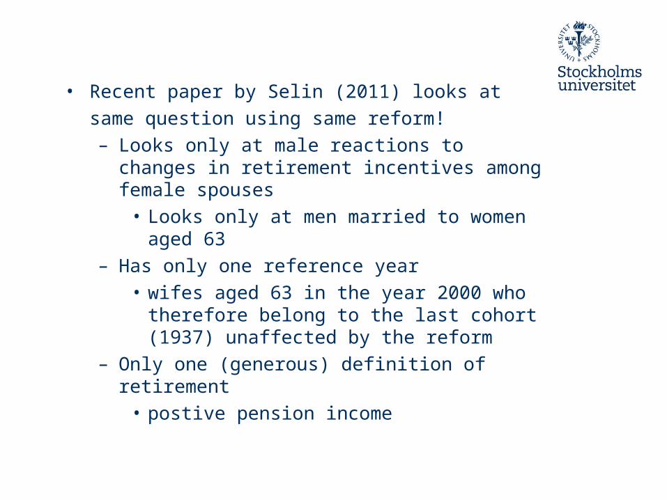
• Recent paper by Selin (2011) looks at same question using same reform!– Looks only at male reactions to changes in

retirement incentives among female spouses• Looks only at men married to women aged 63

– Has only one reference year • wifes aged 63 in the year 2000 who therefore

belong to the last cohort (1937) unaffected by the reform

– Only one (generous) definition of retirement • postive pension income

The 2000 Pension Reform

• The 2000 pension reform introduced a defined contribution system in comparison to the old defined benefit system

• The new national pension system consists of three parts; income pension (Notional Defined Contribution), premium pension and guarantee pension– plus occupation-based and private pensions.

• Contributions to income pensions are recorded in individual accounts which represent individual claims to future pension benefits. – Annual contributions to the NDC are used to finance

current pension benefit obligations as in a pay-as-you-go system.

The 2000 Pension Reform increased work incentives• Income and premium pension are based on lifetime

earnings including pensionable income from sickness benefits, parental leave, unemployment insurance, studies (with national student loans) and military service.

• Pensions can be withdrawn at the earliest from age 61 but pensions are reduced until the age of 65 at which time they are adjusted back to regular levels. – There is no upper age limit for commencing pension

payments (in previous system, work after age 70 did not lead to higher pensions).

• In the new system, pensions are higher the later they are withdrawn due to a lower number of years with expected pension payments and higher lifetime contributions.

Old System

• Folkpension (independent of previous income) and supplementary benefit (ATP): ATP = 0.60*BPA*ATP points

ATP points = (pensionable income-BPA)/BPA (BPA=36,600 SEK in year 2000)

–ATP points earned during 15 highest years of income since age 16 (or average over available years)–Pensions could be withdrawn from beginning of the month an individual turns 61 (with a permanent reduction by 0.5% for each month left until age 65 –Postponement possible until age 70 (with 0.7 percent permanent increase for each postponed month)

Distribution of pension across new (orange) and old (grey) system by cohort

Two approaches:

1. Graph actual and simulated retirement and joint retirement behavior under various assumptions in order to see how much of actual behavior can be explained by the average behavior of individuals (in a given cohort, sector etc)

2. Difference-in-difference & triple difference analyses of reform effect – Compare cohorts affected by the reform with those not

affected by the reform before and after the reform kicks in (2000).

– Given treatment effect on own retirement behavior, estimate treatment effect of having a spouse affected by the reform in comparison to having a spouse not affected by the reform before and after the reform kicks in.

Difference-in-difference strategy (and triple difference)

– Also use the fact that local public sector workers simultaneously experienced a reform of occupational pensions towards a defined contribution system (enhancing the effect of the general pension reform in comparison to private sector workers).

– Use reform to instrument effect of spousal retirement on own retirement, focusing only on those not directly affected by the reform (?)

Data

• IFAU database– Information on all individuals aged 16-65 from 1985-

2000 and all individuals aged 16-74 from 2001-2007• Information on employment, sector, income,

education from 1985• Information on various sources of pension

income from 1990: early retirement, folkpension, ATP, disability pensions (old system) and income pension, premium pension, occupational pensions (aggregated), guarantee pension (new system)

Restrictions• Couples who have the same spouse throughout the

observation period– Depart from LOUISE data (1990-2008)– Keep only cohorts born 1930-1950– Missing are couples where:

• one spouse falls outside LOUISE age range• dies during the observation period• Family identification is missing• No match between LOUISE and Employment (Sys)

data

• 54% of over 3 million individuals observed are with same spouse throughout the observation period– 24% constantly single– 18% change spouse– 4% ?

Defining Retirement

• Four definitions of retirement:

1. No work: income equal to zero

2. Some pension: sum of all pension sources greater than zero

3. More pension: sum of income plus sick benefits less than sum of pension income

4. Permanent drop: Permanent drop in income (including sick benefits) of at least 33% from one year to the next– This measure (& no work) can be measured from 1985

• Today focus on ”drop income” and ”some pension”

Defining sector of employment

• No direct information on occupational pensions available

• Two definitions (based on data from 1985-2008) of four defined sectors:– State, County, Municipality, Other (Private Swedish,

Private Foreign)

1. Sector with majority of observations before the age of 60

2. Sector with maximum income before the age of 60

Panel 1985-2008 of individuals and their spouses born 1934-1941

Female Male Birth year 1938 1937 Retired (year 2000, cohort 1937): No work 49.3 39.5 Some pension 68.0 64.6 More pension 58.5 52.7 Drop income 66.2 60.9 Sector (based on income) State 10,1 16,5 Municipality 32,0 12,8 County 13,8 2,4 Other 39,7 67,1 Sector (based on no. of observations) State 9,8 15,4 Municipality 31,2 12,1 County 13,8 2,2 Other 42,2 70,2 Joint Retirement (drop income) Same year 9,34 Within 1 year 22,9 Within 2 years 34,0 Within 5 years 59,1

0.1

.2.3

.4.5

.6.7

.8.9

1C

_re

t_dr

opi

nc

45 50 55 60 65 70age

36 37

ret_dropinc woman kom1

0.1

.2.3

.4.5

.6.7

.8.9

1C

_re

t_dr

opi

nc

45 50 55 60 65 70age

36 37

ret_dropinc woman other1

0.1

.2.3

.4.5

.6.7

.8.9

1C

_re

t_dr

opi

nc

45 50 55 60 65 70age

37 38


0.1

.2.3

.4.5

.6.7

.8.9

1C

_re

t_dr

opi

nc

45 50 55 60 65 70age

37 38


0.1

.2.3

.4.5

.6.7

.8.9

1C

_re

t_dr

opi

nc

45 50 55 60 65 70age

38 39


0.1

.2.3

.4.5

.6.7

.8.9

1C

_re

t_dr

opi

nc

45 50 55 60 65 70age

38 39


Own retirment by cohort & sector

0.1

.2.3

.4.5

.6.7

.8.9

1C

_re

t_dr

opi

nc

45 50 55 60 65 70age

39 40


0.1

.2.3

.4.5

.6.7

.8.9

1C

_re

t_dr

opi

nc

45 50 55 60 65 70age

39 40


.1.2

.3.4

.5.6

.7.8

.91

C_r

et_

dro

pin

c

45 50 55 60 65 70age

40 41


0.1

.2.3

.4.5

.6.7

.8.9

1C

_re

t_dr

opi

nc

45 50 55 60 65 70age

40 41


0.1

.2.3

.4.5

.6.7

.8.9

1C

_re

t_dr

opi

nc

45 50 55 60 65 70age

36 37

ret_dropinc man kom2

0.1

.2.3

.4.5

.6.7

.8.9

1C

_re

t_dr

opi

nc

45 50 55 60 65 70age

36 37

ret_dropinc man other2

0.1

.2.3

.4.5

.6.7

.8.9

1C

_re

t_dr

opi

nc

45 50 55 60 65 70age

37 38


0.1

.2.3

.4.5

.6.7

.8.9

1C

_re

t_dr

opi

nc

45 50 55 60 65 70age

37 38


0.1

.2.3

.4.5

.6.7

.8.9

1C

_re

t_dr

opi

nc

45 50 55 60 65 70age

38 39


0.1

.2.3

.4.5

.6.7

.8.9

1C

_re

t_dr

opi

nc

45 50 55 60 65 70age

38 39


0.1

.2.3

.4.5

.6.7

.8.9

1C

_re

t_dr

opi

nc

45 50 55 60 65 70age

39 40


0.1

.2.3

.4.5

.6.7

.8.9

1C

_re

t_dr

opi

nc

45 50 55 60 65 70age

39 40


0.1

.2.3

.4.5

.6.7

.8.9

1C

_re

t_dr

opi

nc

45 50 55 60 65 70age

40 41


0.1

.2.3

.4.5

.6.7

.8.9

1C

_re

t_dr

opi

nc

45 50 55 60 65 70age

40 41


Joint Retirement: Females

0.0

1.0

2.0

3.0

4

55 60 65 70age

m_bothclose m_pbothcloser1m_pbothcloser3

Both Retired within a year Women 1935

0.0

1.0

2.0

3.0

4

55 60 65 70age


Both Retired within a year Women 1940

Joint Retirement: Males

0.0

1.0

2.0

3.0

4.0

5

55 60 65 70age


Both Retired within a year Men 1935

0.0

2.0

4.0

6

55 60 65 70age


Both Retired within a year Men 1940

Joint Retirement: Females (incl. Sector)

0.0

1.0

2.0

3.0

4

55 60 65 70age

m_bothclose_restr m_pbothcloser2m_pbothcloser4 m_pbothcloser2_secm_pbothcloser4_sec

Both Retired within a year Women 1935 SEC

0.0

1.0

2.0

3.0

4.0

5

55 60 65 70age



Joint Retirement: Males (incl. Sector)

0.0

2.0

4.0

6

55 60 65 70age


Both Retired within a year Men 1935 SEC

0.0

2.0

4.0

6

55 60 65 70age



Joint Retirement, Same Year

0.0

05

.01

.01

5

55 60 65 70age

m_bothret_restr m_pbothretr2m_pbothretr4 m_pbothretr2_secm_pbothretr4_sec

Both Retired in same year Women 1935 SEC

0.0

05

.01

.01

5.0

2

55 60 65 70age


Both Retired in same year Women 1940 SEC

0.0

05

.01

.01

5.0

2.0

25

55 60 65 70age


Both Retired in same year Men 1935 SEC

0.0

05

.01

.01

5.0

2.0

25

55 60 65 70age


Both Retired in same year Men 1940 SEC

Joint retirement within one year: some pension definition

0.0

1.0

2.0

3.0

4

55 60 65 70age



0.0

1.0

2.0

3.0

4.0

5

55 60 65 70age



0.0

2.0

4.0

6.0

8

55 60 65 70age



0.0

2.0

4.0

6.0

8

55 60 65 70age



Probability of retirement X years apart:

.04

.06

.08

.1.1

2

-4 -2 0 2 4diff_year

diff_scale diff_r0_scalediff_r1_scale diff_r3_scale

Probability of retirement x years apart Women 1935

.04

.06

.08

.1



Probability of retirement x years apart Women 1940

.04

.06

.08

.1



Probability of retirement x years apart Men 1935

.04

.05

.06

.07

.08

.09



Probability of retirement x years apart Men 1940

Difference in difference estimation of reform effect (change in own pension incentives) on retirement probability (treatment= birth year>1937, post= year>2000)

Females Males (1) (2) (3) (4) Cohorts 1930-1950 1934-1941 1930-1950 1934-1941 Treatment*Post -.276***

(.001) -.065***

(.001) -.195***

(.001) -.064***

(.001) Treatment -.286***

(.001) -.134***

(.001) -.367***

(.001) -.158***

(.001) Post 1.035***

( .001) 1.020***

( .002) 1.050***

(.001) 1.044***

(.001) R2 0.30 0.46 0.39 0.51 Observations 6,518,815 2,659,022 6,539,423 2,860,731 Standard errors clustered at individual level. All estimations control for a full set of year dummies plus all relevant direct effects and double interaction effects. *** denotes significance at one percent level, ** at five percent level and * at ten percent level.

Males: Females

F( 13,350562) = 4608.31 F( 13,350107) = 4701.79 Prob > F = 0.0000 Prob > F = 0.0000

-.2

-.1

0.1

.2E

stim

ate

d co

effi

cien

t

1931 1933 1935 1937 1939 1941 1943 1945 1947 1949Birth year

-.2

-.1

0.1

.2E

stim

ate

d co

effi

cien

t

1931 1933 1935 1937 1939 1941 1943 1945 1947 1949Birth year

Difference in difference estimation of reform effect on pension probability (birth year*post interactions, reference year = 1930)

Triple difference estimation of direct reform effect on retirement

Females Males (1) (2) (3) (4) Cohorts 1930-1950 1934-1941 1930-1950 1934-1941 Treatment*Post*Public -.144***

(.002) -.074***

(.003) -. 101***

(.003) -. 077***

(.004) Treatment*Post -. 212***

(.002) -. 033***

(.003) -. 180***

(.001) -. 052***

(.002) R2 0.31 0.47 0.39 0.51 Observations 6,518,815 2,659,022 6,539,423 2,860,731 Standard errors clustered at individual level. All estimations control for a full set of year dummies plus all relevant direct effects and double interaction effects. *** denotes significance at one percent level, ** at five percent level and * at ten percent level.

Triple difference estimation of reform effect (birth year*local public sector*post)

Males: Females:

F( 13,350562) = 91.59 F( 13,350107) = 208.89 Prob > F = 0.0000 Prob > F = 0.0000

-.15

-.1

-.05

0.0

5E

stim

ate

d co

effi

cien

t

1931 1933 1935 1937 1939 1941 1943 1945 1947 1949Birth year

-.2

-.15

-.1

-.05

0.0

5E

stim

ate

d co

effi

cien

t

1931 1933 1935 1937 1939 1941 1943 1945 1947 1949Birth year

OLS Estimation of Spousal Retirement on Individual Retirement

Female Male (1) (2) (3) (4) 1930-1950 1934-1941 1930-1950 1934-1941 Spousal Retirement

.176*** (.005)

.147*** (.007)

.163*** (.005)

.130*** (.006)

R2 0.38 0.49 0.45 0.52 Observations 6,518,815 2,659,022 6,539,423 2,860,731 Clusters 440 168 440 168 Standard errors clustered on cohort*spousal cohort. All estimates control for cohort, spousal cohort, direct reform effects, sector, spousal sector and year dummies. *** denotes significance at the one percent level.

Triple difference estimation of SPOUSAL reform effect on retirement probabilities (given own reform effect)

Females Males (1) (2) (3) (4) Cohorts 1930-1950 1934-1941 1930-1950 1934-1941 Spouse_Treatment*Post*Spouse_Public -.028

(.019) -.018 (.016)

-.029 (.021)

-.016 (.013)

Spouse_Treatment*Post -.104*** (.007)

-.024*** (.005)

.025 (.016)

.009 (.009)

R2 0.33 0.47 0.40 0.51 Observations 6,518,815 2,659,022 6,539,423 2,860,731 Clusters 1693 653 1688 670 Standard errors clustered on cohort*sector*spousal cohort*spousal sector. All estimations control for a full set of year dummies plus all relevant direct effects and double interaction effects (own and spouses). *** denotes significance at one percent level, ** at five percent level and * at ten percent level.

Triple difference estimation of SPOUSAL reform effect on retirement probabilities (spouse birth year*spouse local public sector*post)

Male Female

F( 13, 1687) = 3.87 F( 13, 1692) = 2.06 Prob > F = 0.0000 Prob > F = 0.0136

-.04

-.02

0.0

2.0

4E

stim

ate

d co

effi

cien

t

1931 1933 1935 1937 1939 1941 1943 1945 1947 1949Spouse's Birth year

-.08

-.06

-.04

-.02

0.0

2E

stim

ate

d co

effi

cien

t


-.06

-.04

-.02

0.0

2E

stim

ate

d co

effi

cien

t


Effects of 'SPOUSAL birth year'-'post reform'-'SPOUSAL local public sector' interactions on retirement probabilities, males

-.06

-.04

-.02

0.0

2.0

4E

stim

ate

d co

effi

cien

t


Effects of 'SPOUSAL birth year'-'post reform'-'SPOUSAL local public sector' interactions on retirement probabilities, females

If we want to use reform as an instrument for spousal retirement, need to

drop those directly affected by the reform (cohorts born after 1937)Distribution of spouses by birth year:

Birth year: Spouses to Females Spouses to Males 1930 14.19 3.22 1931 14.63 4.68 1932 14.56 6.10 1933 13.00 7.15 1934 11.76 8.42 1935 9.89 9.28 1936 7.59 10.22 1937 5.24 10.23 1938 3.26 9.67 1939 2.00 8.37 1940 1.25 6.49 1941 0.77 4.84 1942 0.51 3.74 1943 0.46 2.66 1944 0.32 1.76 1945 0.22 1.15 1946 0.14 0.79 1947 0.10 0.51 1948 0.06 0.34 1949 0.03 0.22 1950 0.02 0.15 Observations 1,785,064 2,762,234

Smaller proportion of spouses to females born after 1937 (these male spouses are older than their wives).

Triple difference estimation of SPOUSAL

reform effect on retirement probabilities,

Individuals born on or before 1937 only:

Male Female

F( 13, 670) = 0.90 F( 13, 602) = 1.40 Prob > F = 0.5554 Prob > F = 0.1520

-.1

-.05

0.0

5.1

Est

ima

ted

coe

ffici

ent


-.4

-.2

0.2

.4E

stim

ate

d co

effi

cien

t


Original idea was to quantify the effect of spousal retirement on own retirement by IV

”If you can’t see the the causal relation of interest in the reduced form, it’s probably not there”

-Angrist and Krueger (2001)

IV estimation of spousal retirement:

• There is a first stage effect of reform on spousal retirement (corr (retirement_s, reform_s)>0)

– Female spouses affected by the reform (triple difference) decrease retirement probabilities by approx. 5.0 percentage points in comparison to female spouses not affected by the reform

– Likewise reform effect on male spouses is - 8.0 pp.

• No reduced form effect of spousal reform on own retirement probabilities (corr

(retirement_i, reform_s)=0)

– Spousal (local public sector reform effect of female (male) spouses on male (female) retirement is -0.4 (0.9) percentage points and not signficant.

Conclusions

• Are there spillover effects of the reform on own

retirement due to changes in spousal retirement

incentives?– Yes, something seems to be happening for those

with spouses born after 1940

• Spill-over effect of reform is likely to work via spousal

retirement but...– can’t as of now use the reform as an instrument to

quantify the causal effect of spousal retirement on own retirement.

Spousal Joint Retirement: A reform based approach to identifying spillover effects Francois Gerard,...

Documents

Transcript of Spousal Joint Retirement: A reform based approach to identifying spillover effects Francois Gerard,...