Spot and Forward Rates under Continuous Compoundinglyuu/finance1/2009/20090304.pdf · Spot and...

Spot and Forward Rates under ContinuousCompounding

• The pricing formula:

P =n∑

i=1

Ce−iS(i) + Fe−nS(n).

• The market discount function:

d(n) = e−nS(n).

• The spot rate is an arithmetic average of forward rates,

S(n) =f(0, 1) + f(1, 2) + · · ·+ f(n− 1, n)

n.

c©2008 Prof. Yuh-Dauh Lyuu, National Taiwan University 26

Spot and Forward Rates under ContinuousCompounding (concluded)

• The formula for the forward rate:

f(i, j) =jS(j)− iS(i)

j − i.

• The one-period forward rate:

f(j, j + 1) = − lnd(j + 1)

d(j).

•

f(T ) ≡ lim∆T→0

f(T, T + ∆T ) = S(T ) + T∂S

∂T.

• f(T ) > S(T ) if and only if ∂S/∂T > 0.

c©2008 Prof. Yuh-Dauh Lyuu, National Taiwan University Page 127

Unbiased Expectations Theory

• Forward rate equals the average future spot rate,

f(a, b) = E[ S(a, b) ]. (14)

• Does not imply that the forward rate is an accuratepredictor for the future spot rate.

• Implies the maturity strategy and the rollover strategyproduce the same result at the horizon on the average.


Unbiased Expectations Theory and Spot Rate Curve

• Implies that a normal spot rate curve is due to the factthat the market expects the future spot rate to rise.

– f(j, j + 1) > S(j + 1) if and only if S(j + 1) > S(j)from Eq. (12) on p. 116.

– So E[ S(j, j + 1) ] > S(j + 1) > · · · > S(1) if and onlyif S(j + 1) > · · · > S(1).

• Conversely, the spot rate is expected to fall if and only ifthe spot rate curve is inverted.


More Implications

• The theory has been rejected by most empirical studieswith the possible exception of the period prior to 1915.

• Since the term structure has been upward sloping about80% of the time, the theory would imply that investorshave expected interest rates to rise 80% of the time.

• Riskless bonds, regardless of their different maturities,are expected to earn the same return on the average.

• That would mean investors are indifferent to risk.


A “Bad” Expectations Theory

• The expected returns on all possible riskless bondstrategies are equal for all holding periods.

• So

(1 + S(2))2 = (1 + S(1)) E[ 1 + S(1, 2) ] (15)

because of the equivalency between buying a two-periodbond and rolling over one-period bonds.

• After rearrangement,

1E[ 1 + S(1, 2) ]

=1 + S(1)

(1 + S(2))2.


A “Bad” Expectations Theory (continued)

• Now consider two one-period strategies.

– Strategy one buys a two-period bond and sells itafter one period.

– The expected return isE[ (1 + S(1, 2))−1 ] (1 + S(2))2.

– Strategy two buys a one-period bond with a return of1 + S(1).

• The theory says the returns are equal:

1 + S(1)(1 + S(2))2

= E

[1

1 + S(1, 2)

].


A “Bad” Expectations Theory (concluded)

• Combine this with Eq. (15) on p. 131 to obtain

E

[1

1 + S(1, 2)

]=

1E[ 1 + S(1, 2) ]

.

• But this is impossible save for a certain economy.

– Jensen’s inequality states that E[ g(X) ] > g(E[X ])for any nondegenerate random variable X andstrictly convex function g (i.e., g′′(x) > 0).

– Use g(x) ≡ (1 + x)−1 to prove our point.


Local Expectations Theory

• The expected rate of return of any bond over a singleperiod equals the prevailing one-period spot rate:

E[(1 + S(1, n))−(n−1)

]

(1 + S(n))−n= 1 + S(1) for all n > 1.

• This theory is the basis of many interest rate models.


Duration Revisited

• To handle more general types of spot rate curve changes,define a vector [ c1, c2, . . . , cn ] that characterizes theperceived type of change.

– Parallel shift: [ 1, 1, . . . , 1 ].

– Twist: [ 1, 1, . . . , 1,−1, . . . ,−1 ].

– · · ·• Let P (y) ≡ ∑

i Ci/(1 + S(i) + yci)i be the priceassociated with the cash flow C1, C2, . . . .

• Define duration as

−∂P (y)/P (0)∂y

∣∣∣∣y=0

.


Fundamental Statistical Concepts


There are three kinds of lies:lies, damn lies, and statistics.

— Benjamin Disraeli (1804–1881)

One death is a tragedy,but a million deaths are a statistic.

— Josef Stalin (1879–1953)


Moments

• The variance of a random variable X is defined as

Var[ X ] ≡ E[(X − E[ X ])2

].

• The covariance between random variables X and Y is

Cov[X, Y ] ≡ E [ (X − µX)(Y − µY ) ] ,

where µX and µY are the means of X and Y ,respectively.

• Random variables X and Y are uncorrelated if

Cov[X, Y ] = 0.

c©2008 Prof. Yuh-Dauh Lyuu, National Taiwan University 8

Correlation

• The standard deviation of X is the square root of thevariance,

σX ≡√

Var[ X ] .

• The correlation (or correlation coefficient) between X

and Y is

ρX,Y ≡ Cov[ X, Y ]σXσY

,

provided both have nonzero standard deviations.


Variance of Sum

• Variance of a weighted sum of random variables equals

Var

[n∑

i=1

aiXi

]=

n∑

i=1

n∑

j=1

aiaj Cov[Xi, Xj ].

• It becomesn∑

i=1

a2i Var[Xi ]

when Xi are uncorrelated.


Conditional Expectation

• “X | I” denotes X conditional on the information set I.

• The information set can be another random variable’svalue or the past values of X, say.

• The conditional expectation E[X | I ] is the expectedvalue of X conditional on I; it is a random variable.

• The law of iterated conditional expectations:

E[ X ] = E[E[ X | I ] ].

• If I2 contains at least as much information as I1, then

E[X | I1 ] = E[ E[X | I2 ] | I1 ]. (16)


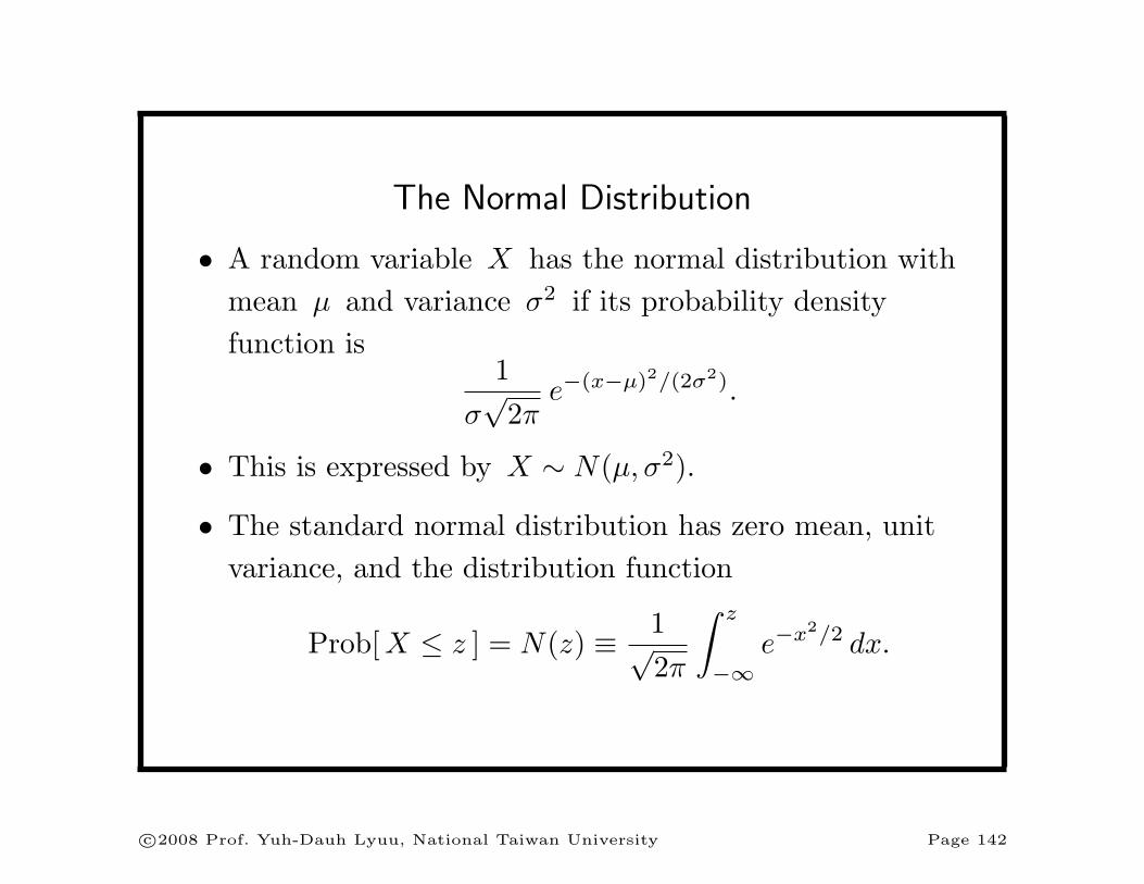
The Normal Distribution

• A random variable X has the normal distribution withmean µ and variance σ2 if its probability densityfunction is

1σ√

2πe−(x−µ)2/(2σ2).

• This is expressed by X ∼ N(µ, σ2).

• The standard normal distribution has zero mean, unitvariance, and the distribution function

Prob[ X ≤ z ] = N(z) ≡ 1√2π

∫ z

−∞e−x2/2 dx.


Moment Generating Function

• The moment generating function of random variable X

isθX(t) ≡ E[ etX ].

• The moment generating function of X ∼ N(µ, σ2) is

θX(t) = exp[

µt +σ2t2

2

]. (17)


Distribution of Sum

• If Xi ∼ N(µi, σ2i ) are independent, then

∑

i

Xi ∼ N

(∑

i

µi,∑

i

σ2i

).

• Let Xi ∼ N(µi, σ2i ), which may not be independent.

• Then

n∑

i=1

tiXi ∼ N

n∑

i=1

ti µi,n∑

i=1

n∑

j=1

titj Cov[ Xi, Xj ]

.

• Xi are said to have a multivariate normal distribution.


Generation of Univariate Normal Distributions

• Let X be uniformly distributed over (0, 1 ] so thatProb[ X ≤ x ] = x for 0 < x ≤ 1.

• Repeatedly draw two samples x1 and x2 from X until

ω ≡ (2x1 − 1)2 + (2x2 − 1)2 < 1.

• Then c(2x1 − 1) and c(2x2 − 1) are independentstandard normal variables where

c ≡√−2(lnω)/ω .


A Dirty Trick and a Right Attitude

• Let ξi are independent and uniformly distributed over(0, 1).

• A simple method to generate the standard normalvariable is to calculate

12∑

i=1

ξi − 6.

• But “this is not a highly accurate approximation andshould only be used to establish ballpark estimates.”a

aJackel, Monte Carlo Methods in Finance (2002).


A Dirty Trick and a Right Attitude (concluded)

• Always blame your random number generator last.a

• Instead, check your programs first.a“The fault, dear Brutus, lies not in the stars but in ourselves that

we are underlings.” William Shakespeare (1564–1616), Julius Caesar.


Generation of Bivariate Normal Distributions

• Pairs of normally distributed variables with correlationρ can be generated.

• X1 and X2 be independent standard normal variables.

• Set

U ≡ aX1,

V ≡ ρU +√

1− ρ2 aX2.

• U and V are the desired random variables withVar[U ] = Var[V ] = a2 and Cov[U, V ] = ρa2.


The Lognormal Distribution

• A random variable Y is said to have a lognormaldistribution if ln Y has a normal distribution.

• Let X ∼ N(µ, σ2) and Y ≡ eX .

• The mean and variance of Y are

µY = eµ+σ2/2 and σ2Y = e2µ+σ2

(eσ2 − 1

),

(18)

respectively.

– They follow from E[ Y n ] = enµ+n2σ2/2.


Option Basics


The shift toward options asthe center of gravity of finance [ . . . ]

— Merton H. Miller (1923–2000)


Calls and Puts

• A call gives its holder the right to buy a number of theunderlying asset by paying a strike price.

• A put gives its holder the right to sell a number of theunderlying asset for the strike price.

• How to price options?


Exercise

• When a call is exercised, the holder pays the strike pricein exchange for the stock.

• When a put is exercised, the holder receives from thewriter the strike price in exchange for the stock.

• An option can be exercised prior to the expiration date:early exercise.


American and European

• American options can be exercised at any time up to theexpiration date.

• European options can only be exercised at expiration.

• An American option is worth at least as much as anotherwise identical European option because of the earlyexercise feature.


Convenient Conventions

• C: call value.

• P : put value.

• X: strike price.

• S: stock price.

• D: dividend.


Payoff

• A call will be exercised only if the stock price is higherthan the strike price.

• A put will be exercised only if the stock price is lessthan the strike price.

• The payoff of a call at expiration is C = max(0, S −X).

• The payoff of a put at expiration is P = max(0, X − S).

• At any time t before the expiration date, we callmax(0, St −X) the intrinsic value of a call.

• At any time t before the expiration date, we callmax(0, X − St) the intrinsic value of a put.


Payoff (concluded)

• A call is in the money if S > X, at the money if S = X,and out of the money if S < X.

• A put is in the money if S < X, at the money if S = X,and out of the money if S > X.

• Options that are in the money at expiration should beexercised.a

• Finding an option’s value at any time before expirationis a major intellectual breakthrough.

a11% of option holders let in-the-money options expire worthless.


20 40 60 80Price

Long a put

10

20

30

40

50

Payoff

20 40 60 80Price

Short a put

-50

-40

-30

-20

-10

Payoff

20 40 60 80Price

Long a call

10

20

30

40

Payoff

20 40 60 80Price

Short a call

-40

-30

-20

-10

Payoff


80 85 90 95 100 105 110 115

Stock price

0

5

10

15

20

Call value

80 85 90 95 100 105 110 115

Stock price

0

2

4

6

8

10

12

14

Put value


Cash Dividends

• Exchange-traded stock options are not cashdividend-protected (or simply protected).

– The option contract is not adjusted for cashdividends.

• The stock price falls by an amount roughly equal to theamount of the cash dividend as it goes ex-dividend.

• Cash dividends are detrimental for calls.

• The opposite is true for puts.


Stock Splits and Stock Dividends

• Options are adjusted for stock splits.

• After an n-for-m stock split, the strike price is onlym/n times its previous value, and the number of sharescovered by one contract becomes n/m times itsprevious value.

• Exchange-traded stock options are adjusted for stockdividends.

• Options are assumed to be unprotected.


Example

• Consider an option to buy 100 shares of a company for$50 per share.

• A 2-for-1 split changes the term to a strike price of $25per share for 200 shares.


Short Selling

• Short selling (or simply shorting) involves selling anasset that is not owned with the intention of buying itback later.

– If you short 1,000 XYZ shares, the broker borrowsthem from another client to sell them in the market.

– This action generates proceeds for the investor.

– The investor can close out the short position bybuying 1,000 XYZ shares.

– Clearly, the investor profits if the stock price falls.

• Not all assets can be shorted.


Payoff of Stock

20 40 60 80Price

Long a stock

20

40

60

80

Payoff

20 40 60 80Price

Short a stock

-80

-60

-40

-20

Payoff


Covered Position: Hedge

• A hedge combines an option with its underlying stock insuch a way that one protects the other against loss.

• Protective put: A long position in stock with a long put.

• Covered call: A long position in stock with a short call.a

• Both strategies break even only if the stock price rises,so they are bullish.

aA short position has a payoff opposite in sign to that of a long

position.


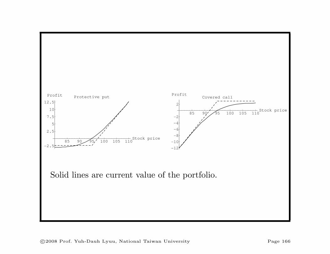
85 90 95 100 105 110Stock price

Protective put

-2.5

2.5

5

7.5

10

12.5

Profit

85 90 95 100 105 110Stock price

Covered call

-12

-10

-8

-6

-4

-2

2

Profit

Solid lines are current value of the portfolio.


Covered Position: Spread

• A spread consists of options of the same type and on thesame underlying asset but with different strike prices orexpiration dates.

• We use XL, XM , and XH to denote the strike priceswith XL < XM < XH .

• A bull call spread consists of a long XL call and a shortXH call with the same expiration date.

– The initial investment is CL − CH .

– The maximum profit is (XH −XL)− (CL − CH).

– The maximum loss is CL − CH .


85 90 95 100 105 110Stock price

Bull spread (call)

-4

-2

2

4

Profit


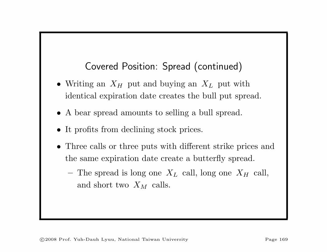
Covered Position: Spread (continued)

• Writing an XH put and buying an XL put withidentical expiration date creates the bull put spread.

• A bear spread amounts to selling a bull spread.

• It profits from declining stock prices.

• Three calls or three puts with different strike prices andthe same expiration date create a butterfly spread.

– The spread is long one XL call, long one XH call,and short two XM calls.


85 90 95 100 105 110Stock price

Butterfly

-1

1

2

3

Profit


Covered Position: Spread (concluded)

• A butterfly spread pays off a positive amount atexpiration only if the asset price falls between XL andXH .

• A butterfly spread with a small XH −XL approximatesa state contingent claim, which pays $1 only when aparticular price results.

• The price of a state contingent claim is called a stateprice.


Covered Position: Combination

• A combination consists of options of different types onthe same underlying asset, and they are either allbought or all written.

• Straddle: A long call and a long put with the samestrike price and expiration date.

• Since it profits from high volatility, a person who buys astraddle is said to be long volatility.

• Selling a straddle benefits from low volatility.

• Strangle: Identical to a straddle except that the call’sstrike price is higher than the put’s.


85 90 95 100 105 110Stock price

Straddle

-5

-2.5

2.5

5

7.5

10

Profit


85 90 95 100 105 110Stock price

Strangle

-2

2

4

6

8

10

Profit


Arbitrage in Option Pricing


All general laws are attended with inconveniences,when applied to particular cases.

— David Hume (1711–1776)


Arbitrage

• The no-arbitrage principle says there is no free lunch.

• It supplies the argument for option pricing.

• A riskless arbitrage opportunity is one that, without anyinitial investment, generates nonnegative returns underall circumstances and positive returns under some.

• In an efficient market, such opportunities do not exist(for long).

• The portfolio dominance principle says portfolio Ashould be more valuable than B if A’s payoff is at leastas good under all circumstances and better under some.


A Corollary

• A portfolio yielding a zero return in every possiblescenario must have a zero PV.

– Short the portfolio if its PV is positive.

– Buy it if its PV is negative.

– In both cases, a free lunch is created.


The PV Formula Justified

P =∑n

i=1 Cid(i) for a certain cash flow C1, C2, . . . , Cn.

• If the price P ∗ < P , short the zeros that match thesecurity’s n cash flows and use P ∗ of the proceeds P

to buy the security.

• Since the cash inflows of the security will offset exactlythe obligations of the zeros, a riskless profit of P − P ∗

dollars has been realized now.

• If the price P ∗ > P , a riskless profit can be realized byreversing the trades.


-6 6 6 6

C1C2 C3

· · · Cn

? ? ? ?C1 C2

C3

· · ·Cn

6P

?P ∗

¾ security

¾ zeros


Two More Examples

• An American option cannot be worth less than theintrinsic value.

– Otherwise, one can buy the option, promptly exerciseit and sell the stock with a profit.

• A put or a call must have a nonnegative value.

– Otherwise, one can buy it for a positive cash flow nowand end up with a nonnegative amount at expiration.


Relative Option Prices

• These relations hold regardless of the probabilisticmodel for stock prices.

• Assume, among other things, that there are notransactions costs or margin requirements, borrowingand lending are available at the riskless interest rate,interest rates are nonnegative, and there are noarbitrage opportunities.

• Let the current time be time zero.

• PV(x) stands for the PV of x dollars at expiration.

• Hence PV(x) = xd(τ) where τ is the time toexpiration.


Put-Call Parity (Castelli, 1877)

C = P + S − PV(X). (19)

• Consider the portfolio of one short European call, onelong European put, one share of stock, and a loan ofPV(X).

• All options are assumed to carry the same strike priceand time to expiration, τ .

• The initial cash flow is therefore C − P − S + PV(X).

• At expiration, if the stock price Sτ ≤ X, the put will beworth X − Sτ and the call will expire worthless.


The Proof (concluded)

• After the loan, now X, is repaid, the net future cashflow is zero:

0 + (X − Sτ ) + Sτ −X = 0.

• On the other hand, if Sτ > X, the call will be worthSτ −X and the put will expire worthless.

• After the loan, now X, is repaid, the net future cashflow is again zero:

−(Sτ −X) + 0 + Sτ −X = 0.

• The net future cash flow is zero in either case.

• The no-arbitrage principle implies that the initialinvestment to set up the portfolio must be nil as well.


Consequences of Put-Call Parity

• There is only one kind of European option because theother can be replicated from it in combination with theunderlying stock and riskless lending or borrowing.

– Combinations such as this create synthetic securities.

• S = C − P + PV(X) says a stock is equivalent to aportfolio containing a long call, a short put, and lendingPV(X).

• C − P = S − PV(X) implies a long call and a short putamount to a long position in stock and borrowing thePV of the strike price (buying stock on margin).


Intrinsic Value

Lemma 1 An American call or a European call on anon-dividend-paying stock is never worth less than itsintrinsic value.

• The put-call parity impliesC = (S −X) + (X − PV(X)) + P ≥ S −X.

• Recall C ≥ 0.

• It follows that C ≥ max(S −X, 0), the intrinsic value.

• An American call also cannot be worth less than itsintrinsic value.


Intrinsic Value (concluded)

A European put on a non-dividend-paying stock may beworth less than its intrinsic value (p. 159).

Lemma 2 For European puts, P ≥ max(PV(X)− S, 0).

• Prove it with the put-call parity.

• Can explain the right figure on p. 159 why P < X − S

when S is small.


Early Exercise of American Calls

European calls and American calls are identical when theunderlying stock pays no dividends.

Theorem 3 (Merton (1973)) An American call on anon-dividend-paying stock should not be exercised beforeexpiration.

• By an exercise in text, C ≥ max(S − PV(X), 0).

• If the call is exercised, the value is the smaller S −X.


Remarks

• The above theorem does not mean American callsshould be kept until maturity.

• What it does imply is that when early exercise is beingconsidered, a better alternative is to sell it.

• Early exercise may become optimal for American callson a dividend-paying stock.

– Stock price declines as the stock goes ex-dividend.


Early Exercise of American Calls: Dividend Case

Surprisingly, an American call should be exercised only at afew dates.

Theorem 4 An American call will only be exercised atexpiration or just before an ex-dividend date.

In contrast, it might be optimal to exercise an American puteven if the underlying stock does not pay dividends.


Convexity of Option Prices

Lemma 5 For three otherwise identical calls or puts withstrike prices X1 < X2 < X3,

CX2 ≤ ωCX1 + (1− ω) CX3

PX2 ≤ ωPX1 + (1− ω)PX3

Hereω ≡ (X3 −X2)/(X3 −X1).

(Equivalently, X2 = ωX1 + (1− ω)X3.)


Option on Portfolio vs. Portfolio of Options

An option on a portfolio of stocks is cheaper than a portfolioof options.

Theorem 6 Consider a portfolio of non-dividend-payingassets with weights ωi. Let Ci denote the price of aEuropean call on asset i with strike price Xi. Then the callon the portfolio with a strike price X ≡ ∑

i ωiXi has a valueat most

∑i ωiCi. All options expire on the same date.

The same result holds for European puts.


Spot and Forward Rates under Continuous Compoundinglyuu/finance1/2009/20090304.pdf · Spot and...

Documents

Transcript of Spot and Forward Rates under Continuous Compoundinglyuu/finance1/2009/20090304.pdf · Spot and...