HAL Id: jpa-00208894https://hal.archives-ouvertes.fr/jpa-00208894

Submitted on 1 Jan 1979

HAL is a multi-disciplinary open accessarchive for the deposit and dissemination of sci-entific research documents, whether they are pub-lished or not. The documents may come fromteaching and research institutions in France orabroad, or from public or private research centers.

L’archive ouverte pluridisciplinaire HAL, estdestinée au dépôt et à la diffusion de documentsscientifiques de niveau recherche, publiés ou non,émanant des établissements d’enseignement et derecherche français ou étrangers, des laboratoirespublics ou privés.

Spontaneous symmetry breaking and bifurcations fromthe Maclaurin and Jacobi ellipsoidsD.H. Constantinescu, L. Michel, L.A. Radicati

To cite this version:D.H. Constantinescu, L. Michel, L.A. Radicati. Spontaneous symmetry breaking and bifurca-tions from the Maclaurin and Jacobi ellipsoids. Journal de Physique, 1979, 40 (2), pp.147-159.�10.1051/jphys:01979004002014700�. �jpa-00208894�

147

Spontaneous symmetry breaking and bifurcationsfrom the Maclaurin and Jacobi ellipsoids

D. H. Constantinescu (*)

European Southern Observatory, 1211 Geneva 23, Switzerland

L. Michel

Institut des Hautes Etudes Scientifiques, 91440 Bures-sur-Yvette, France

and

L. A. Radicati (**)

CERN, 1211 Geneva 23, Switzerland

(Reçu le 7 juin 1978, accepté le 26 octobre 1978)

Résumé. 2014 L’état d’équilibre d’un fluide tournant soumis à son interaction gravitationnelle est déterminé par deséquations non linéaires. Les solutions d’équilibre, paramétrées par le carré du moment cinétique, présentent desbifurcations accompagnées de brisures de symétrie. D’hypothèses très générales on déduit des règles de sélectionconcernant les brisures de symétrie qui peuvent apparaître dans ce problème. Les bifurcations sont du même typeque celles à la Landau qui apparaissent dans les transitions de phase du second ordre. La méthode est illustrée parl’exemple simple d’un fluide incompressible animé d’une rotation globale et une nouvelle famille infinie de bifur-cations est trouvée. Cependant les règles de sélection sont plus générales ; elles s’appliquent aussi aux modèles quireprésentent la rotation d’une étoile de façon plus réaliste.

Abstract. 2014 The equilibrium of a rotating self-gravitating fluid is governed by non-linear equations. The equili-brium solutions, parametrized in terms of the angular momentum squared, exhibit the phenomenon of bifurcation,accompanied by spontaneous symmetry breaking. Under very general assumptions, a set of selection rules can bederived, which drastically restrict the patterns of symmetry breaking that are allowed to appear. Bifurcations ofthis kind are similar to second-order phase transitions à la Landau. The method is illustrated by the simple exampleof an incompressible fluid in rigid rotation. However, the selection rules are more general; they apply also tomodels which approximate a rotating star more realistically.

LE JOURNAL DE PHYSIQUE TOME 40, FÉVRIER 1979,

Classification

Physics Abstracts02.20 - 03.40 - 98.10

1. Introduction. - The phenomenon of bifurcationof solutions, encountered in non-linear eigenvalueproblems, is closely related to that of spontaneoussymmetry breaking. Numerous examples in bifur-cation theory [1] suggest that, when a bifurcationoccurs in a stationary problem, the symmetry of thenew solution is lower than the symmetry of the solu-tion it bifurcates from, even though the symmetryof the governing equations remains unchanged [2].We propose to examine this connection within the

framework of an old problem of astrophysical interest :the equilibrium of rotating fluid masses held togetherby gravitation [3]. In the particular case of an incom-pressible, homogeneous fluid in rigid rotation, the

equations of hydrostatic equilibrium form a set ofnon-linear equations for the surface which boundsthe fluid at equilibrium. These equations dependupon the parameter J2, the square of the angularmomentum, and are invariant under the group D ooh [4].For 0 J2 0.384 436 [5], the equilibrium surfaceis also invariant under D.h (Maclaurin ellipsoids).As the angular momentum squared increases beyondthe critical value 0.384 436, new solutions appear,whose invariance groups are subgroups of D.h.The first of these is the set of Jacobi ellipsoids, inva-

Article published online by EDP Sciences and available at http://dx.doi.org/10.1051/jphys:01979004002014700

148

riant under the subgroup D2h of Dooh. Other solutionsare known, bifurcating both from the Maclaurin andJacobi sequences, but a rigorous classification of allpossible solutions is still missing.The aim of this paper is to give such a classification,

using as a criterion the type of symmetry breaking thataccompanies the bifurcation. More precisely, we

address ourselves to the following problem : givena solution of the equations of hydrostatic equilibriumand its isotropy group, find the possible isotropygroups of the solutions which bifurcate from it, andthe values of J2 at which the bifurcations appear.Our investigation is strictly limited to the equilibriumof the fluid mass ; stability is not examined here [6].The plan of the paper is the following. In section 2

we write the equation of hydrostatic equilibrium,then derive from it a linearized equation for thedeformation by which, starting from a given equili-brium solution, new solutions may be obtained.

Polynomial deformations of ellipsoidal solutions arediscussed in detail. In section 3 the group-theoreticaldescription of symmetry breaking is used to obtain,under very general assumptions, the list of all possiblepatterns of symmetry breaking that may accompanybifurcations from the Maclaurin and Jacobi sequences.These results are used in section 4 to compute explicitlythe bifurcations corresponding to polynomial defor-mations of the lowest degree associated with eachtype of allowed symmetry breaking. In addition to theknown bifurcations, a new infinite family of bifur-cations from the Maclaurin sequence is found,corresponding to a D.h breaking. The connectionwith the theory of second-order phase transitionsand the general applicability of the method to caseswhich approximate more realistically a rotating star(compressible fluid with differential rotation) are

discussed in section 5. The parametrization of ellip-soidal solutions is described in the appendix.

2. Basic équations ; polynomial solutions. - Con-sider a homogeneous incompressible fluid of givenmass and volume, rotating rigidly about a fixed axiswith angular momentum J. We will assume that in thecoordinate system in which the fluid is at rest the onlyforces are the gravitational and centrifugal forces.The fluid is assumed to occupy a connected volume,bounded by the surface

S(x) = 0 . (2.1)

We adopt the convention that S(x) > 0 inside thefluid.

2.1 EQUILIBRIUM EQUATION. - In the corotatingsystem, the equations of hydrodynamics reduce to theequations of hydrostatic equilibrium [5]

is the sum of the gravitational and centrifugal poten-tials. The gravitational potential, satisfying Poisson’sequation

and the boundary conditionis given by

Taking the 3rd axis along J, the centrifugal potential is

where

is the corresponding moment of inertia.Equation (2.2) must be integrated subject to the

boundary condition

whence it follows that the fluid boundary is an equi-potential :

This is an equation for the function S which determinesthe boundary at equilibrium, dependent upon theparameter J2. We shall call equation (2.9) the equi-librium equation and its solutions S(x ; J2) equilibriumsolutions.

.

Let us show that an ellipsoid is an equilibriumsolution. We set

where

Then, in terms of the functions (Xil...in(81, 82’ 83) definedby equation (A. 3),

and equation (2.9) yields

149

from which we deduce

Equation (2.15) always admits the trivial solutionel = 82. However, if the angular momentum squaredexceeds the critical value 0.384 436, a new solution,with 81 * 82, appears. The continuous set of equi-librium solutions obtained by varying continuouslythe angular momentum [by equation (2.14) the e’sare functions of j2] form the Maclaurin (81 = 82)and Jacobi (e1 * B2) sequences. These are illustratedin figure 1, where the squares of the polar and equa-torial eccentricities

of the equilibrium ellipsoid are plotted versus the

angular momentum squared.

Fig. 1. - Ellipsoidal equilibrium solutions. Polar eccentricitysquared (a) and equatorial eccentricity squared (b) versus angularmomentum squared. Solid curves : Maclaurin sequence. Dashedcurves : Jacobi sequence. The dots indicate the Maclaurin-Jacobibifurcation (see table II) and the next bifurcation on each branch(see table III).

2.2 BIFURCATION EQUATION. - We want to findwhether new solutions of the equilibrium equation,différent from ellipsoids, exist, and to determine thevalues of J2 at which they bifurcate from the Mac-laurin and Jacobi sequences.

Given an equilibrium solution S(x ; J2), new solu-tions may be obtained from it by applying to the fluida static deformation. Such a deformation is conve-

niently described in terms of a vector field ;(x),giving the displacement of the fluid element at point x :

where À is a real parameter. In particular, the fluidsurface (2. 1) will be deformed into

where

Only first-order deformations will be considered-herethen

We require that the deformations leave invariantthe density, the centre of mass and the angular momen-tum of the fluid. To first order in À, the displacementmust then satisfy the conditions

n being the unit vector along the rotation axis. A

displacement field satisfying equations (2.21)-(2.23)will be called admissible. Since the defining equationsare linear, the set of admissible §’s is a vector space 9J..Under the displacement (2.17) the potential changes

according to

where

The term VF represents the change in the gravitationalpotential due to the deformation of the surface. Thereis no corresponding term for the centrifugal potentialsince, to first order in À, the moment of inertia remainsconstant as a consequence of eq. (2.23).

In order that the deformed fluid configuration bein equilibrium, eq. (2.9) must hold for the modifiedpotentiel of eq. (2.24) and the deformed surface (2.20).

150

This yields the condition

Equation (2.26) represents a linear equation for thefirst-order displacement field § which deforms theinitial equilibrium configuration of the fluid,S(x ; J2) = 0, into a new equilibrium configuration,S(x, J2) = 0. Equation (2.26) will be referred to asthe bifurcation equation.

An admissible displacement field § will be calledtrivial if, on the surface S(x ; J2) = 0, it lies in the

tangent plane to this surface, i.e. if

The set of trivial §’s forms a subspace 9Y, of Va. Wecan now prove the following.

Indeed, integrating by parts and using eqs. (2.21)and (2.28), we have

From this theorem it follows immediately that a

trivial displacement satisfies identically the bifurcationequation. Such trivial solutions do not deform the

original surface and will be discarded. More precisely,we will look for solutions of eq. (2.26) in the quotientspace COa/COt. Such solutions will be called bifurcationsolutions.

2. 3 POLYNOMIAL DEFORMATIONS OF ELLIPSOIDS. -

We will now examine in detail the case in which thefluid surface is an ellipsoid (Maclaurin or Jacobi)given by eq. (2.10), and the displacement field §is a polynomial in x. We denote by

a polynomial scalar field which, on the ellipsoidS(x ; J’) = 0, is proportional to the normal compo-nent of §. Equation (2.19) then reads

so the polynomial P is the surface deformation. Weremark that for the ellipsoidal surface (2. 10), equa-tion (2.30) implies P(O; J2) = 0.We now want to find a vector deformation §

corresponding to a given surface deformation P.

Since every polynomial P has a unique decompositionas a sum of homogeneous polynomials Pn of degree nwe choose

Like the §’s, the surface deformations P have to

satisfy a set of admissibility conditions :

The integrals are over the domain S(xi ; J2) > 0.One can verify that eqs. (2.33)-(2.36) are equivalentto eq. (2 . 21 )-(2 . 23). In particular the two eqs. (2.35),(2. 36) express the conservation of angular momentum.

Equation (2.30) associates to every trivial vectorinformation a trivial surface deformation Pt whichvanishes on the surface S(x ; J2) = 0. Hence

One can now prove the following.Theorem : If P is a polynomial of given degree and

parity, then VF[EP] is also a polynomial of the samedegree and parity.The proof is elementary, but rather involved;

we sketch below the main steps. Since F[§] is a linearfunctional, it is sufficient to prove the theorem for thecase in which the components of § are monomialsof degree n - 1, viz. of the form

Then, the theorem holds for the first few values ofn > 1 [7], which suggests a proof by induction. So,assuming it to be true for a degree n - 1, we will showthat the same follows for degree n. We use the identity

151

where Cn is a coefficient, Rn-2j(x) is a polynomial ofdegree lower than or equal to n - 2 j, and fIn/2]denotes the largest integer smaller than or equal to n/2.This enables us to write

Now we use in the right-hand side the equation [8]

[here f(x) is an arbitrary function], and the fact [9]that Fr[S"J is a polynomial of degree 2 n + 2. Thetheorem then follows from eq. (2.40) by simple powercounting.

Let us denote by en) the vector space of polynomialsof degree n and parity Ç. In section 3 we will show thatthe polynomial deformation P belongs to such a

space iS(n). The importance of the above theoremresides in having established that the correspondence

is a homomorphism of (T into ("’). Consequently,the bifurcation equation (2.26) may be regarded asan equation for the polynomial deformation P.

This is a convenient point of view for the discussionof symmetry breaking, so let us write explicitly thebifurcation equation in this form. For the ellipsoidalequilibrium solutions, eqs. (2.3) to (2.15) imply thatthe potential at equilibrium is

Equation (2.27) then becomes

where I[P] is defined by eq. (2.42). [For polynomialsof degree n 4 this f-transform can be calculatedexplicitly from Chandrasekhar’s identities [7].] Onthe other hand, for polynomial deformations eq. (2.26)is satisfied if and only if

R(x) being an arbitrary polynomial. Solving thebifurcation equation in the form (2.45) amountsnow to the identification of polynomial coefficients.The term bifurcation solution will be used for a

solution P(x ; J2) of the eigenvalue equation (2.45) in the quotient space S/S, where Ta and Tt are, in thevector space of polynomials P, the subspaces of theadmissible and trivial polynomials respectively.

3. Sélection rules for symmetry breaking. - Wenow proceed to discuss the symmetry properties of theequilibrium and bifurcation equations and their non-trivial solutions, in order to determine the patterns ofsymmetry breaking that may appear at bifurcations.This will be done by using the powerful formalism ofgroup theory, which only recently has been appliedto bifurcation problems [23, 24]. We will brieflyrecall some basic notions [10], then apply them to ourspecific problem.

3. 1 GROUP-T’HEORETICAL DESCRIPTION OF SYMME-TRY BREAKING. - We consider an equation havingthe general form

#(U, Jl) = 0 , (3.1)

where u(x) is the unknown function, and y is a realparameter ; Ç/ is a smooth map, otherwise arbitrary.Equation (3.1) is assumed to be covariant under a

group G, in the following sense. Let g be an element ofG, and T(g) the 3 x 3 matrix which represents itsaction on the three-dimensional Euclidean space :

Then, its action on any function u(x) is represented bya linear operator 0 fi defined by

Equation (3. 1) is said to be covariant under G if theaction of this group commutes with the map rji, i.e. if

An immediate consequence of covariance is that,if u is a solution of eq. (3.1) for some value of theparameter J1, then Og u is also a solution for the same p.The set of all solutions obtained from u by the actionof G is called the orbit of u [11].The solutions of eq. (3.1) are, in general, not

invariant under G ; this is the phenomenon of spon-taneous symmetry breaking. Given a solution u,the elements of G which transform u into itself form a

subgroup H of G called the isotropy group, or littlegroup, of u. If u has the isotropy group H, thenu’ = tJg u has the isotropy group H’ = gHg-1, i.e. Hand H’ are conjugated subgroups of G. Therefore,the isotropy group H of a given solution u charac-terizes, up to a conjugation in G, the whole orbit of u,which will be denoted by the symbol G/H. The fore-going discussion referred to a fixed u, but now it canbe extended to all values of J1. The set of all orbits ofthe same type (i.e. having the same little group, up to aconjugation) is called a stratum. A symmetry-changingbifurcation point at a certain critical value of the

parameter J1 corresponds to a critical orbit markingthe boundary between two adjacent strata.

Let us now apply these considerations to the equi-

152

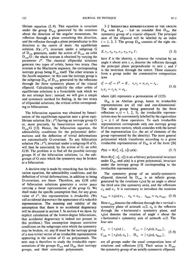
librium equation (2.9). This equation is covariantunder the group Dooh, generated by the rotationsabout the direction of the angular momentum, thereflexion through a plane containing this direction,and the reflexion through a plane perpendicular to thisdirection at the centre of mass. An equilibriumsolution S(x ; J2), invariant under a subgroup Gof D ooh generates, under the action of D ooh, an orbitDooh/G ; the whole stratum is obtained by varying theparameter J2. The classical ellipsoidal solutions

generate two types of orbits, hence two strata. Onestratum is the Maclaurin sequence, the correspondingisotropy group being D ooh itself. The other stratum isthe Jacobi sequence ; in this case the isotropy group isthe subgroup D2h of Dooh, generated by the reflexionsthrough the three symmetry planes of the triaxial

ellipsoid. Calculating explicitly the other orbits ofequilibrium solutions is a formidable task which wedo not attempt hère ; instead, we will give a simpleand systematic method for finding, in the two strataof ellipsoidal solutions, the critical orbits correspond-ing to bifurcations.

The bifurcation equation was obtained by lineari-zation of the equilibrium equation near a given equi-librium solution S(x ; J2) having an isotropy group Gor, more precisely, by linearization near an orbit

D ooh/G [12]. Hence, the bifurcation equation, the

admissibility conditions for the polynomial defor-mations and the definition of trivial deformationsare automatically G-covariant. To any bifurcationsolution P(x ; J2), invariant under a subgroup H of G,will then be associated, by the action of G, an orbitG/H. The problem is to find all the possible isotropygroups H of the bifurcation solutions, i.e. the sub-

groups of G onto which the symmetry may be brokenat a bifurcation.

A decisive step is made by remarking that the bifur-cation equation, the admissibility conditions, and thedefinition of trivial deformations, in addition to beingG-covariant, are linear. Therefore, any G/H orbitof bifurcation solutions generates a vector spacecarrying a linear representation of the group G. Weshall make the specific assumption that, for any givenvalue of J2, this representation is irreducible. (Wecall accidental degeneracy the appearance of a reduciblerepresentation. The meaning and validity of the

assumption that there is no accidental degeneracywill be discussed in section 5. In section 4 we show, byexplicit calculation of the lowest-degree bifurcations,that accidental degeneracy is indeed not present inthis problem.) This assumption imposes restrictiveconditions on the subgroups onto which the symmetrymay be broken, viz. any H must be the isotropy groupof a non-trivial vector of an irreducible representationappearing in the action of G on polynomials. Thenext step is therefore to study the irreducible repre-sentations of the groups D.h and D2h, their isotropygroups, and their covariant polynomials.

3.2 IRREDUCIBLE REPRESENTATIONS OF THE GROUPS

D2h AND D oob. - Let us consider first D2h, the

symmetry group of a triaxial ellipsoid. The principalaxes of the ellipsoid will be labelled by an indexi = 1, 2, 3. The group D2h consists of the eight ele-ments

here E is the identity, ri denotes the rotation by anangle 1t about axis i, ai denotes the reflexion throughthe principal plane perpendicular to axis i, and 1is the inversion through the centre. These elements

; form a group under the commutative compositionlaws

where (ijk) represents a permutation of (123).D2h is an Abelian group, hence its irreducible

representations are all real and one-dimensional.The whole group being generated by the threereflexions ui (i = 1, 2, 3), the irreducible represen-tations may be conveniently labelled by the eigenvalues(j = ± 1 of these operators. To each irreducible

representation corresponds only one isotropy groupH of non-zero vectors, which coincides with the kernelof the representation (i.e. the set of elements of thegroup represented by the identity). The most generalpolynomial which transforms according to a givenirreducible representation of D2h is of the form [26]

Here 0(xf, x’, x23) is an arbitrary polynomial invariantunder D2h, and cp(x) is a given polynomial, invariantunder the isotropy group H corresponding to theirreducible representation.The symmetry group of an axially-symmetric

ellipsoid, denoted by Dooh, is an infinite group,

generated by the rotations r3(w) by an angle w aboutthe third axis (the symmetry axis), and the reflexionsU3 and 61. It is customary to introduce the notation

Here (J v(a» denotes the reflexion through the « vertical »symmetry plane of azimuth w/2, Uh is the reflexion

through the « horizontal » symmetry plane, and

rh(w) denotes the rotation of angle n about the« horizontal » symmetry axis of azimuth w/2. Thefour sets

are all groups under the usual composition laws ofrotations and reflexions [13]. Their union is D ooh,the symmetry group of an axially-symmetric ellipsoid.

153

Each of the groups Coov, Cooh and Doo is a propersubgroup of Dooh; Coo is a proper subgroup of eachof them. All the other proper subgroups of D ooh arefinite.The irreducible representations of Dooh are all real,

either two-dimensional or one-dimensional. In thetwo-dimensional ones the generating elements are

represented as follows :

Here m is a positive integer (m = 1, 2, ...), and(3 = ± 1. These representations are convenientlylabelled by the doublet (m, (3). The two representationsthat would obtain from eq. (3.loj for m = 0 arereducible; they decompose into one-dimensionalirreducible representations in which the generatingelements are now represented as follows :

Here Cl = ± 1 distinguishes between the two irre-

ducible representations corresponding to m = 0 andthe same (3. The one-dimensional irreducible repre-sentations will be labelled by the triplet (m = 0, (3’ (l)-To each one-dimensional irreducible representation

of D ooh corresponds only one isotropy group H, whichcoincides with the kernel of the representation ; this isnot true for the two-dimensional representations,for which H is determined only up to a conjugation,and is larger than the kernel. The most general poly-nomial which transforms according to a given irre-ducible representation of D ooh is of the form

Here d = 1, 2 is the dimension of the representation,Oi(X2 + x2, x23) are arbitrary polynomials invariantunder D ooh, and (pi(x) are given polynomials, invariantunder the corresponding isotropy group H.

In table 1 we list all the irreducible representationsof the groups D2h and Dooh. For both groups the headentries indicate the irreducible representations(labelled as described above), the correspondingisotropy groups H (denoted by their classical names[4]), and the explicit form of the invariant polynomials(p [26].

3.3 SELECTION RULES. - These results may besummarized in a set of selection rules for symmetrybreaking at bifurcations, indicating which patternsof symmetry breaking are forbidden under the assump-tion that accidental degeneracy does not occur. Thecontents of these selection rules, which are presentedschematically in table I, is discussed below.

Table I. - Irreducible representations of the D2h andDooh groups.

1) The only subgroups of D2h and Dooh that areallowed as isotropy groups of bifurcation solutionsare those listed in table 1 ; any other subgroup is for-bidden. This eliminates exactly half of the subgroupsof D2h, viz. Cs(k), C2(k), S2 and Cl = { E }, (k = 1, 2,3). In the case of Dooh the forbidden subgroups are Coo,Cmv, Cmh, S2m and Dm (m = 1, 2, ...). It is interestingto note that the forbidden isotropy groups are alwayssmaller than the allowed ones. In other words, theabsence of accidental degeneracy leads in a naturalway to minimal symmetry breaking.

2) When only polynomial deformations are consi-dered, the subgroups Cooh and D 00 of Dh are alsoforbidden, because they do not appear in the actionof the group on polynomials.Symmetry considerations do not impose any restric-

tion on the degree of the polynomial deformation P(x) ;indeed, in eqs. (3.7) and (3.12) the 9’s are arbitrarypolynomials. However, once the degree n has beenfixed, new selection rules come into force :

3) All the isotropy groups for which the ç’s areof degree greater than n are forbidden. (Example :Dmh and Dm-1,d are forbidden if m > n.)

4) All the irreducible representations of D2h andDooh have definite parity = ± 1 (the parity of theç’s in table I). This forbids the isotropy groups withthe wrong parity, i.e. with , =1= ( - 1)", eliminatinghalf of the subgroups in table I, both for D2h and Dooh.The selection rules represent a powerful instrument,

which drastically reduces the list of possible types ofsymmetry breaking at bifurcations. Whether theallowed types of breaking actually occur is a dynamicalquestion which can be answered only by explicitlysolving the bifurcation equation. If there is no solution,the bifurcation, although allowed kinematically (i.e.from the point of view of symmetry breaking), is

dynamically forbidden (i.e. is incompatible with theequation of hydrostatic equilibrium).

4. Lowest-degree polynomial bifurcations. - Fromthe foregoing discussion the following practical pro-cedure for the calculation of bifurcations has emerged.Given the isotropy group G of the original equilibrium

154

solution [12], table 1 lists all the possible isotropygroups H of the bifurcation solutions. Once the degreen of the polynomial deformation has been chosen,the most general form of an H-invariant admissible Pis found from eqs. (3.7) or (3.12), table I, and

eqs. (2.33) to (2.36). The r-transform of P can becalculated explicitly [7] ; then, identification of thecoefficients in the bifurcation equation (2.45) yields

a system of linear homogeneous algebraic equationsfor the set of coefficients { À } which parametrize P.The bifurcation solution is found by solving this

system.This procedure is now illustrated by explicit compu-

tation of the bifurcations corresponding to polyno-mial deformations of the lowest degree compatiblewith each type of allowed symmetry breaking. For

Table II. - Second-degree bifurcations from the Maclaurin and Jacobi sequences.

(*) This spurious solution does not correspond to a bifurcation ; see the text.

Table III. - Third-degree bifurcations from the Maclaurin and Jacobi sequences.

155

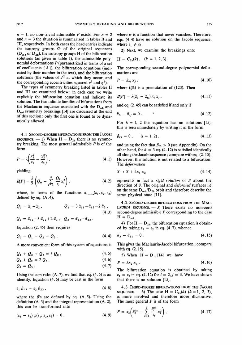
n = 1, no non-trivial admissible P exists. For n = 2and n = 3 the situation is summarized in tables II andIII, respectively. In both cases the head entries indicatethe isotropy groups G of the original sequences(D ooh or D2h), the isotropy groups H of the bifurcationsolutions (as given in table I), the admissible poly-nomial deformations P (parametrized in terms of a setof coefficients { À }), the bifurcation equations (indi-cated by their number in the text), and the bifurcationsolutions (the values of J2 at which they occur, andthe corresponding eccentricities squared e2 and n2).The types of symmetry breaking listed in tables II

and III are examined below ; in each case we writeexplicitly the bifurcation equation and indicate itssolution. The two infinite families of bifurcations fromthe Maclaurin sequence associated with the Dmh andDmd symmetry breakings [14] are discussed at the endof this section ; only the first one is found to be dyna-mically allowed.

4.1 SECOND-DEGREE BIFURCATIONS FROM THE JACOBI

SEQUENCE. - 1) When H = D2h there is no symme-try breaking. The most general admissible P is of theform

yielding

where, in terms of the functionsdefined by eq. (A. 4),

Equation (2. 45) then requires

A more convenient form of this system of equations is

Using the sum rules (A. 7), we find that eq. (4. 5) is anidentity. Equation (4.6) may be cast in the form

where the B’s are defined by eq. (A. 5). Using thedefinition (A. 3) and the integral representation (A. 2),this can be transformed into

where (p is a function that never vanishes. Therefore,eqs. (4.4) have no solution on the Jacobi sequence,where 81 =F 82.

2) Next, we examine the breakings onto

The corresponding second-degree polynomial defor-mations are

where (ijk) is a permutation of (123). Then

and eq. (2.45) can be satisfied if and only if

For k = 1, 2 this equation has no solutions [15],this is seen immediately by writing it in the form

Pi3 = 0 , (i = 1, 2), (4.13)

and using the fact that Bi3 > 0 (see Appendix). On theother hand, for k = 3 eq. (4.12) is satisfied identicallyall along the Jacobi sequence ; compare with eq. (2.15).However, this solution is not related to a bifurcation.The deformation

represents in fact a rigid rotation of S about thedirection of J. The original and deformed surfaces lieon the same Dooh/D2h orbit and therefore describe thesame physical state [11].

4.2 SECOND-DEGREE BIFURCATIONS FROM THE MAC-LAURIN SEQUENCE. - 3) There exists no non-zero

second-degree admissible P corresponding to the caseH = Dooh.

4) For H = D2h, the bifurcation equation is obtain-ed by taking 81 = 82 in eq. (4.7), whence

This gives the Maclaurin-Jacobi bifurcation ; comparewith eq. (2.15).

The bifurcation equation is obtained by taking8 1 = 92 in eq. (4.12) for i = 2, j = 3. We have shownthat there is no solution [15].

4.3 THIRD-DEGREE BIFURCATIONS FROM THE JACOBI

SEQUENCE. - 6) The case H = C2v(k) (k = 1, 2, 3),is more involved and therefore more illustrative.The most general P is of the form

156

with the restriction

imposed by the conservation of the centre of mass.We note that when

equation (4.17) reduces to a trivial deformation.

Calculating the f-transform [7] one obtains

where Qi(k), (i = 0, 1, 2, 3), are linear forms in the threeindependent parameters Â(’), (m = 1, 2, 3). Equation(2.45) requires that

written in the form

these relations form a system of three linear, homo-geneous equations for the three parameters Àm(k).Explicitly, they may be written as

where

Equations (4.23) have a non-zero solution if and onlyif

This condition turns out to be satisfied identicallynot only all along the Jacobi sequence, but also for anyvalues of the e’s. Indeed, using the sum rules (A. 7)one finds that the sum of the three columns in thedeterminant in eq. (4.25) is zero :

The origin of this disease is traced down to the presencein our equations of the trivial deformation (4.19).To cure it, we may choose anyone of the Â’s equalto zero, which is equivalent to removing from eq.(4.17) a trivial deformation proportional to xk S [16].For the remaining deformation to be non-trivial, allthe second-order minors of the determinant in eq.(4.25) must then vanish. Omitting the proofs, whichare elementary but tedious, let us state the main

results. All the second-order minors Dl:l are pro-portional :

The y’s are functions of the e’s that never vanish.

Equation (4.25) then factorizes into

where, by the sum rules (A. 7), X(k) is identically zero.Removing this spurious zero, the bifurcation is givenby the equation

In terms of the eigenvalues of the matrix Clm(k), all thisboils down to the fact that one eigenvalue is identicallyzero, whereas the zeros of the other two eigenvaluesare given by eq. (4.29). Once a solution of this equationis known, the coefficients À,k) (up to an arbitrarycommon additive constant) are found as the compo-nents of the corresponding eigenvector of Cl(.k). Anumerical calculation shows that, on the Jacobi

sequence, eq. (4.29) admits a solution only [15] fork = 1 ; the corresponding eigenvector is

This is the bifurcation to the famous pear-shapedfigure of Poincaré, invariant under C2,(I).

whence

Equation (2.45) is satisfied only if

or equivalently

Using the positivity of the B’s, one concludes that theD2 bifurcation does not occur [15].

4.4 THIRD-DEGREE BIFURCATIONS FROM THE MAC-

LAURIN SEQUENCE. - 8) When H = Coov, the third-degree admissible P is obtained by setting À1 = Â2,91 = 82 in eq. (4.17) for k = 3. It is sufficient, there-fore, to look for solutions of eq. (4.29) in this parti-cular case; there are none [15].

9) For H = Dih [14], the polynomial deformationis again a special case of eq. (4.17) : À1 1 = À2, el = 92,and k = 1. Then, eq. (4.29) factorizes into

157

where

Each factor in eq. (4.35) yields one solution. Theassociated types of symmetry breaking are found bycomputing the corresponding eigenvectors. The solu-tion

represents the breaking onto D1h.10) The bifurcation to H = D3h is obtained from

the other solution of eq. (4. 35) :

11) For H = D2d, the bifurcation equation is

(4.34), with E1 = 82. There exists no bifurcation ofthistype[15].

4.5 HIGHER-DEGREE BIFURCATIONS FROM THE MAC-LAURIN SEQUENCE. - Finally, let us examine thebifurcations from the Maclaurin sequence accompa-nied by symmetry breaking onto the subgroups Dmnor Dmd (m > 2) [14]. As before, the discussion isrestricted to the lowest-degree polynomial deforma-tion compatible with the breaking.

where cm(x) = Re (xi + ’X2)’, one obtains

Here lm) stands for â 1...1 with m indices 1 and A;r isa function that never vanishes. To satisfy eq. (4.41)one must have

The bifurcation equation (4.42) has one solution foreach m > 2. The solution for the first few values of mare given in table IV. It seems that only the m = 3 and

Table IV. - Lowest-degree bifurcations from theMaclaurin sequence corresponding to symmetry break-ing onto Dmh groups.

m = 4 bifurcations were known : see [19] chap. 6 ;see however [30] for a related work.

13) When H = D.d, the lowest-order polynomialdeformation is

yielding

where â 13 + 1 stands for a1...13 with m indices 1 andone index 3. The bifurcation equation is

In terms of the positive fi’s defined by eq. (A. 5), thismay be written in the form

showing that there are no Dmd bifurcations [15].

5. Concluding remarks. - In the scheme presentedhere, the calculation of bifurcations is based on twogeneral assumptions : the absence of accidental

degeneracy, and the arbitrary choice of the degreeof the polynomial deformation. We would like to adda few comments on the meaning and justification ofthese assumptions.

It has been shown [27] that the Maclaurin-Jacobibifurcation is similar to second-order phase transi-tions, as described by the Landau theory [28]. We nowextend this point of view to an arbitrary bifurcation.Let us consider the fluid in a configuration boundedby the surface S(x) = 0, where S(x) is a polynomialin x. Its energy is a functional of S, depending also onthe angular momentum squared ; we denote it byE[S] (J’). For each value of J’, the equilibriumsolutions are given by the minima of E, the lowestminimum corresponding to stable equilibrium. Thecovariance group of the equilibrium equation, Dooh,acts on the space T of real polynomials by an ortho-gonal representation. Thus, T is a real Hilbert space,and the energy becomes a real-valued function on S ;we denote it by E(J’, §), where § stands for the vectorcoordinate of S in T.

Let now S(x, J’) be an equilibrium solution, andthe subgroup G of Dooh its isotropy group. We denoteby T(G) the representation of G on T, which can alwaysbe decomposed into irreducible representations. Cor-respondingly, T decomposes into a direct sum of

subspaces ; here a labels the factorial represen-tations (direct sums of equivalent irreducible repre-sentations) appearing in the decomposition of T(G),and n labels the irreducible representations insideeach factorial representation. An expansion of theenergy in the coordinates of S, around the minimumcorresponding to the equilibrium solution considered,is of the form

158

Here Ç0153, is the vector component of § in the subspaceT(an) ; for simplicity, the minimum of the energy hasbeen chosen as origin. There are no linear terms in theexpansion (5.1), and the quadratic terms may alwaysbe brought to normal form (a sum of squares) by anorthogonal transformation.The point § = 0 will no longer be a minimum if one

of the coefficients of the quadratic terms vanishes,i.e. if for a certain label (an) one has

This equation determines the subspace T(0152n) in whichthe bifurcation occurs, and the corresponding criticalvalue of the angular momentum. Of course, one cannota priori rule out the possibility that eq. (5.2) holdsimultaneously for two, or more, values of a. However,satisfying several different conditions with one valueof the parameter J2 would be a casual coincidence(accidental degeneracy) which, if it happened, wouldrequire a separate discussion. We have shown byexplicit calculation that this is not the case in our

problem.The label n, which distinguishes between equivalent

irreducible representations, is related to the degreeof the arbitrary polynomials 0 in eqs. (3. 7) and (3.12) ;it is convenient to identify it with the degree of thepolynomial deformation P. Intuitively, a large angularmomentum is needed to sustain against gravity aconfiguration bounded by a complicated surface.

Hence, for a given a, the critical values of J’, givenby eq. (5.2), are expected to be increasing functionsof n.

Assuming that an appropriate algorithm, is avai-lable one could go beyond the linearized equation(2.27), and determine not only the bifurcation points,but the complete sequences branching off. The wholegame could then be played again, to find the bifur-cation points on these new sequences, etc. In theabsence of accidental degeneracy, minimal symmetrybreaking is expected at each bifurcation. The proce-dure must eventually terminate when the isotropygroup of the bifurcation solution reduces trivially tothe identity. At this point all the symmetry of theproblem has disappeared, and the method loses allits predictive power.

Actually, the method becomes inapplicable evenbefore all the symmetry has gradually been lost bythe mechanism of spontaneous symmetry breaking.The cause is the onset of dynamical instability, whichleads to non-stationary phenomena [6]. (In our

problem it would lead to the fragmentation of thefluid mass.) Then, dynamical details such as fluctua-tions, impurities, etc., become important, and theensuing symmetry breaking is typically maximal.Unlike stationary bifurcations, dynamical instabilitiesare perhaps similar to first-order phase transitions.

In order to simplify the numerical calculationswhich illustrate the method, homogeneity, incômpres-

sibility and rigid rotation have been assumed, therebyreducing the degrees of freedom of the fluid mass tothe degrees of freedom of its surface. In order to builda more realistic model for a rotating star, these assump-tions must be relaxed. New degrees of freedom canthen be excited, such as changes of volume and internalmotions. Nevertheless, the equations of motion remainDooh-covariant, and the foregoing discussion of sym-metry breaking - in particular table I and the selectionrules - remain unaffected.The authors are grateful to one of the referees for

his remarks and for pointing out other works [29],[30], [31] where group theory methods are appliedto astrophysical problems.

Appendix

Parametrization of ellipsoïdal solutions. - Let thefluid have mass m and, in the corotating system, bebounded by an ellipsoidal surface of semi-axes a,,a2, a3. We adopt a special system of units, in whichthe unit of length is a = (al a2 a3)1/3, and the unitof moment of inertia is (2/5) ma2 ; angular momentumsquared is measured in units (12/25) Gm3 a, potentialin units 3 Gmla, and energy in units (3/5) Gm2/a,where G is the gravitational constant. Then, the

energy of the fluid is

where cl, 92, B3 are the squares of the semi-axes, J2is the square of the angular momentum, and

A convenient description of the fluid’s propertiesat equilibrium is given in terms of the infinite set ofparameters [17]

where nk is the number of times the index k appearsin the string il, ..., i". In particular, the f-transformof a polynomial is again a polynomial (see section 2),whose coefficients are simple functions of the a’s [7].Equation (2.12), which gives the gravitational poten-tial at an internal point of a fluid, is such an example.To simplify certain calculations, it is useful to

introduce the quantities

159

and

Combining the definition (A. 3) and the integralrepresentation (A. 2), it is easy to show that the B’sare always positive, a property which is needed in ’ certain proofs.A set of useful identities satisfied by the a’s is

obtained by observing that cxit...in is a homogeneousfunction of degree - (n + 1/2), i.e. that

Applying Euler’s theorem one obtains

Equations (A. 7) will be referred to as sum rules.

i Finally, let us remark that the equilibrium equa-tions (2.14) and (2.15) can be obtained by requiringthat the energy (A .1) have a local extremum withrespect to variations of the e’s, subject to the addi-tional conditions (2 .11 ).

References and footnotes

[1] See, for example [18].[2] This spontaneous symmetry breaking is to be distinguished

from the more familiar dynamical symmetry breaking(symmetry breakdown in the equations of motion).

[3] A detailed presentation of the problem, with references, is

found in [19], [20] ; these two references are almost

complementary. From 1969 on a string of papers havebeen published on this subject, mostly in The Astrophy-sical Journal. They are not relevant to our point of viewhere, and are too numerous to be cited only for comple-teness.

[4] For a description of the symmetry groups appearing in thispaper see, for example [21].

[5] Throughout this paper, all quantities are dimensionless. Theyrepresent the values of the corresponding dimensionalquantities, measured in appropriate natural units, whichare described in the Appendix.

[6] See, for example, [19], [22], and references therein. [7] See [19], Ch. 3, Theorems 3, 14, 15 and 16.[8] See [19], Ch. 3, Lemma 8.[9] See [19], Ch. 3, Theorem 13.

[10] For details see [24], [25].[11] Equation (3.1) must be regarded as the equation of motion

of a physical system, depending upon the external para-meter 03BC. Its solutions describe the dynamical states ofthe system. The covariance under G means that allsolutions belonging to the same orbit represent the samephysical state, seen from different reference frames. Onlyin presence of a perturbation destroying the G-covariance(e.g. impurities, defects, fluctuations, etc.) would one beable to distinguish physically between the solutions

belonging to the same orbit.[12] We are interested in the bifurcations from the ellipsoidal

equilibrium solutions, so G is either D~h or D2h.[13] See [21]; in particular note that r3(03C9) 03C31 = 03C31 r3(- 03C9),

whereas 03C33 commutes with any rotation r3(03C9).[14] For m = 1, the notations Dmh and Dmd are not appropriate;

the symmetry pattern is better described by the alternativenotations D1h = C2v(03C9) and D1d = C2h(03C9), where 03C9

denotes an arbitrary direction in the (x1, x2) plane. Thecase m = 1 is examined separately.

[15] This verifies the theorem of reference [31]; the plane x3 = 0(orthogonal to the angular momentum) is always a

symmetry plane of the figure of equilibrium.[16] A similar trick has probably been used, but not mentioned,

in Chandrasekhar’s calculation of this bifurcation ([19],p. 109). His eqs. (52) to (54) do not follow from eq. (51).The numerical result, however, is correct.

[17] See [2], section 2.1.

[18] KELLER, J. B. and ANTMAN, S., Bifurcation Theory and Non-linear Eigenvalue Problems (New York : Benjamin) 1969.

[19] CHANDRASEKHAR, S., Ellipsoidal Figures of Equilibrium (NewHaven : Yale University Press) 1969.

[20] APPELL, P., Traité de mécanique rationnelle (Paris : Gauthier-Villars) 1932, Vol. IV, fasc. I (1932), Fasc. II (1937).

[21] LANDAU, L. D. and LIFSHITZ, E. M., Quantum Mechanics(Oxford : Pergamon Press) 1965, Ch. XII.

[22] LYTTLETON, R. A., The Stability of Rotating Liquid Masses(Cambridge : University Press) 1953.

[23] RUELLE, D., Arch. Rat. Mech. Anal. 51 (1973) 136.[24] SATTINGER, D., SIAM J. Math. Anal. 8 (1977) 179.

[25] MICHEL, L., J. Physique Colloq. 36 (1975) C7-41.[26] MICHEL, L., Group Theoretical Methods in Physics (Proc. 5th

Intern. Colloq.), New York, Academic Press (1977) p. 75.[27] BERTIN, G. and RADICATI, L. A., Astrophys. J. 206 (1976) 815.[28] LANDAU, L. D. and LIFSHITZ, E. M., Statistical Physics

(Oxford, Pergamon Press) 1958, Ch. XIV.[29] DYSON, F. J., J. Math. Mech. 18 (1968) 91.[30] PERDANG, J., Astrophys. Space Sci. 1 (1968) 355; see also

mimeographed notes GAT-IR 51, Istituto di Astronomia,Universita di Padova, Italy.

[31] LICHTENSTEIN, Gleichgewichtfiguren rotierender Fluessigkeiten(Springer) 1933.