Spline Interpretation ABC

Introduction and outline

Based mostly on Wikipedia

Spline Interpretation

• Spline is a flat flexible strip of thin narrow piece of wood, metal, or plastic used in drawing curved.

• Mathematically, spline means curve fitting mostly using certain piecewise low degree polynomials.

• The main reason to use low degree polynomial is to avoid Runge’s phenomenon.

Runge’s Phenomenon

2

i n

1Given a function : f(x) = .

1 25 x

We want to intropolate at equal spaced points:

2x = 1 + i 1 , for i = 1, 2, ..., n+1 , with polynomial p (x).

n

For n = 1 ; we have only two points to define a str

aight line.

For n = 2 ; we have three point and a quadratic equation, ...

Runge’s PhenomenonRed: data; blue: 5th order; green: 9th order

Runge’s Phenomenon

nn 1 x 1

It can be shown that

f ( x ) p ( x ) .

One of the solutions to the Runge's phenomenon

is to use spline with piecewise low degree polynomials

and not try to fit the whole range. E

lim max

ven in the local

fitting, low degree should be preferred.

Definition of Spline

0 1 2 n 1 n

0 0 1

1 1 2

n 1

Given n+1 data points (known as knots), x, such that

x < x < x < .... < x < x ,

a pline function S(x) of degree k is

S ( x ) x x , x

S ( x ) x x , xS( x ) =

:

S ( x )

n 1 n

i

'

x x , x

where each function S (x) is a polynomial of degree k.

Linear Spline

i 1 ii i i

i 1 i

i 1 i

Linear spline is the simplest spline with data points

connected by straight lines:

y y S (x) = y + x x .

x x

As spline must be continuous at each data points, we must have

S (x) = S (x

i i 1i 1 i i 1 i i 1 i

i i 1

i 1 ii i i i i

i 1 i

) for all i = 1, 2, ....n-1.

Indeed, we have

y y S (x ) = y + x x = y

x x

y y S (x ) = y + x x

x x

i = y

Quadratic Spline

2

2i 1 ii i i i i

i 1 i

i

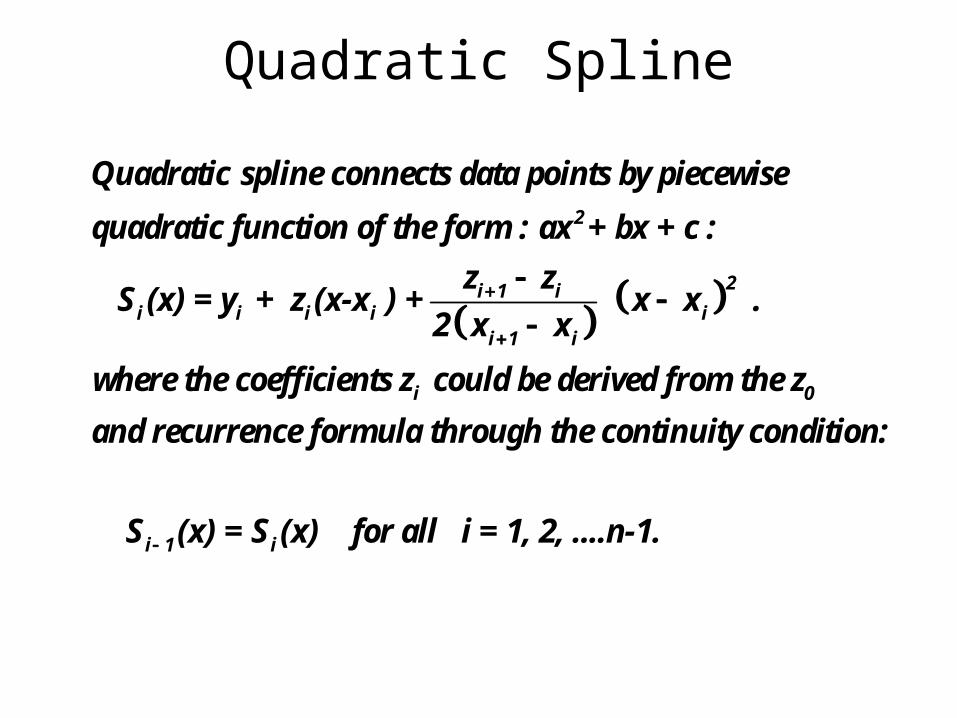
Quadratic spline connects data points by piecewise

quadratic function of the form : ax + bx + c :

z z S (x) = y + z (x-x ) + x x .

2 x x

where the coefficients z could be derived from the z

0

i 1 i

and recurrence formula through the continuity condition:

S (x) = S (x) for all i = 1, 2, ....n-1.

Quadratic Spline

2i i 1i 1 i i 1 i 1 i i 1 i i 1 i

i i 1

2i 1 ii i i i i i i i i

i 1 i

i i 1i i 1

i i 1

Indeed, we have

z z S (x ) = y + z (x x ) + x x = y

2 x x

z z S (x ) = y + z ( x x ) + x x = y

2 x x

This gives

y y z = z + 2 ,

x x

which is ap

proximately a running derivative.

Cubic Spline

3 2

i i

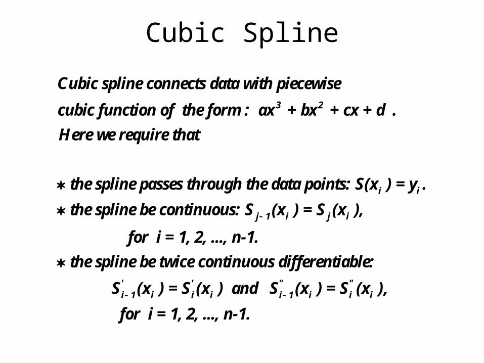
Cubic spline connects data with piecewise

cubic function of the form : ax + bx + cx + d .

Here we require that

the spline passes through the data points: S(x ) = y .

the spline be continuous:

j 1 i j i

' ' " "i 1 i i i i 1 i i i

S (x ) = S (x ),

for i = 1, 2, ..., n-1.

the spline be twice continuous differentiable:

S (x ) = S (x ) and S (x ) = S (x ),

for i = 1, 2,

..., n-1.

Cubic Splinei

i i

For n+1 points, we have n piecewise cubic functions S (x).

We need 4n conditions to determine the polynominals.

The conditions we have are these:

S(x ) = y at all points give

j 1 i j i

S (x ) = S (x ) at interior points

for i = 1, 2, ..., n-1only give

the twice continuous different

n+1condition

iable also a

s

n-1

t int

conditi

erior points

ons

' ' " "i 1 i i i i 1 i i i S (x ) = S (x ) and S (x ) = S (x ),

for i = 1, 2, ..., n-1, give

So we have a total of conditions

2n -2 c

only.

onditions

4n - 2 We are two rt sho

.

Cubic Spline

' '0 k

" "0 n

These give us freedom to choose:

1. Clamped cubic spline:

S (x ) = ; S (x ) = , with and given.

2. Natural spline:

S (x ) = S (x ) = 0.

3. Periodic

2 fre

cubi

e conditio

c spline:

ns

S(

' ' " "0 n 0 n 0 nx ) = S(x ); S (x ) = S (x ) ; S (x ) = S (x )

Hermite Spline

3 2 200

3 2 210

3 2 201

3 2 211

'00 10

The 4 hermite are these:

h (t) = 2t + 3t +1 = (1+2t)(1-t)

h (t) = t - 2t + t = t (1-t)

h (t) = - 2t +3t = t (3-2t)

h (t) = t - t = t (t-1)

Note: h (0) = 1; h

basis functi

(0) = 1

ons

; '01 11h (1) = 1; h (1) = 1.

As these values are unity, we can use them to control

values of any function with initial and end points values

and slopes.

Hermite Spline

Hermite spline

0 0 1 1

00 0 10 0 01 1 11 1

k 1 k

For given P , M and P , M values, at the initial and

end points, we can have a polynomial as,

p(t) = h (t) P + h (t) M + h (t) P + h (t) M

The interpolation in the interval (x x ) shold

00 0 10 0 01 1 11 1

kk 1 k

be

p(t) = h (t) P + h (t) M + h (t) P + h (t) M ,

x xwhere h = x x and t =

h h

.h

Hermite spline

k 1 k k k 1

kk 1 k k k 1

In Hermite spline, the choice of the slope could be selected

sensibly according to our need:

1. Finite difference spline is the simplest:

P P P P m = , for all internal poin

2 x x 2 x x

ts.

Hermite spline

k 1 k 1

kk 1 k 1

2. Cardinal Spline

P P m = 1 c , with 1 < c < 1 as tension parameter.

2 x x

The parameter,c, controls the length of the tangent.

The case, c = 0, is known as Catmull-Rom spline

Fritsch, F . N .; Carlson, R. E . 1980 " Monotone Piecewise Cubic Interpolation" .

SIAM Journal on Numerical Analysis

,

.

3. Monotonic spline

MatLab 'pchip' is monotonic spline based on Fritsch and Carlson.

17 2 : 238 – 246 .

Hermite spline

• In general, cubic spline does not guarantee monotonicity even for monotonic data.

• Hermite monotonic spline, however, guarantees monotonicity between data points.

• The advantage is the elimination of overshoots.• The prices to pay are these:

– we no longer have the smoothness of continuity in curvature and

– we have to inject another subjective idea of monotonic and/or variations.

Comparisons between Cubic Natural and Hermite Splines

An Example

Data

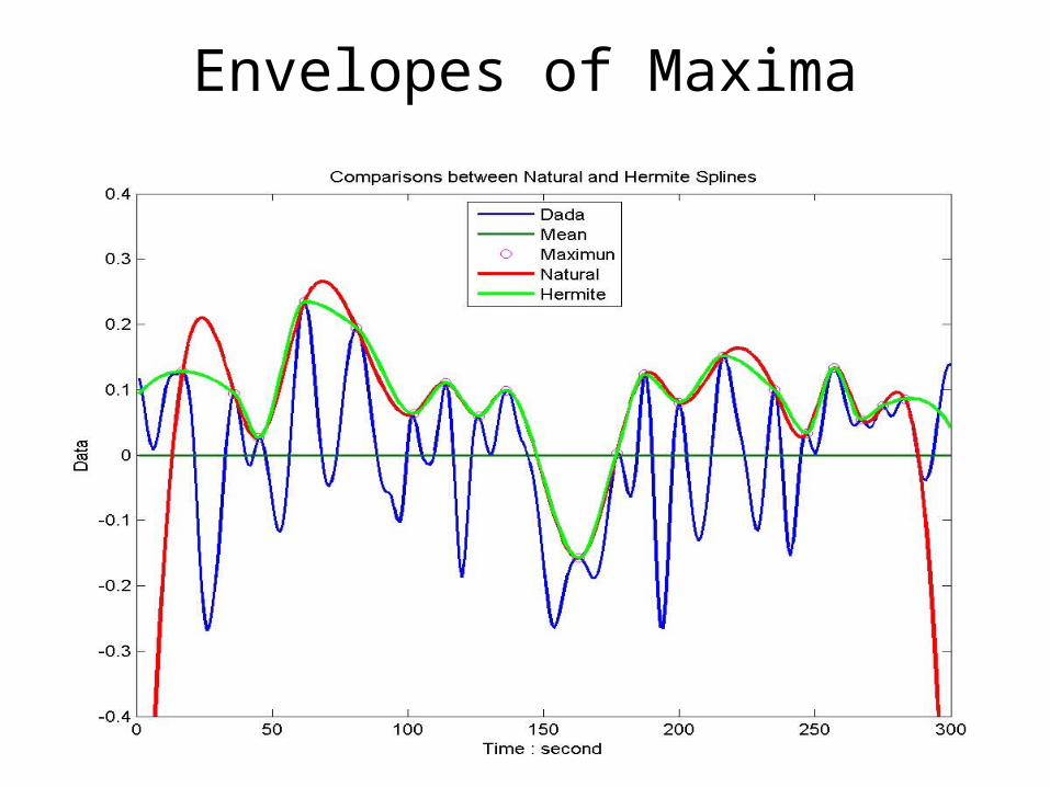
Envelopes of Maxima

Envelopes of Minima

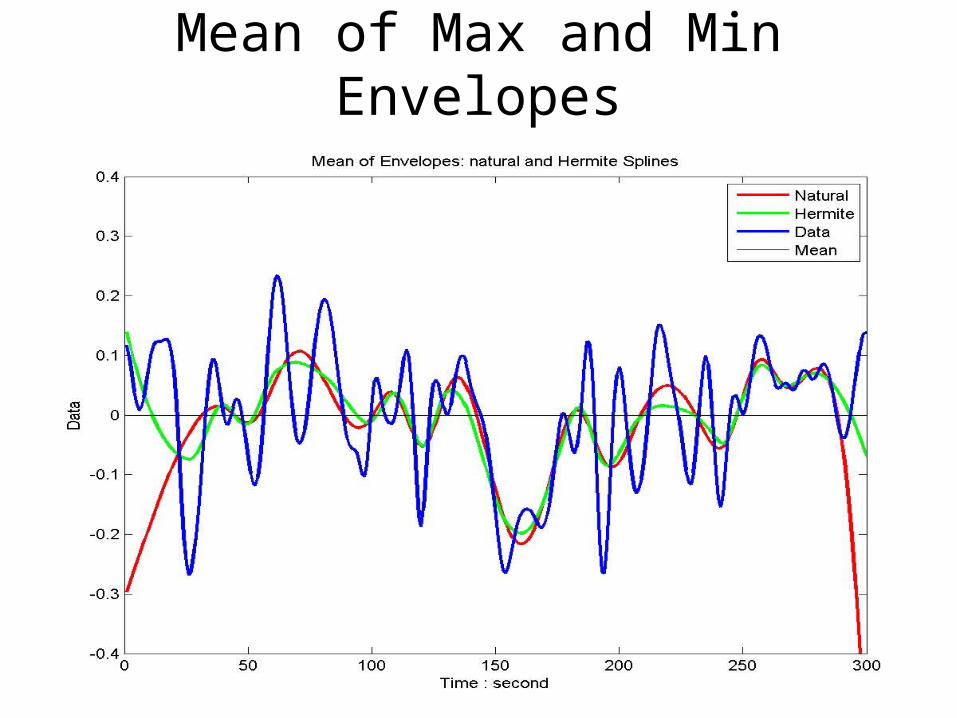
Mean of Max and Min Envelopes

Difference between Mean of Max and Min Envelopes

First Proto-IMF

B-Spline

Something used extensively by Computer Aided Design (CAD),

but we have found limited use of it.

Bézier CurveA Bezier curve is a basis function dependent parametric curve

determined by a a set of control points (or control polygon).

It has the following properties:

1. The basis functions are real

2. The degree of the polynomial is one less thanthe control points.

3. The first and last points of the curve and control points coincide.

4. The tangents at the beginning and end point coincide with the

control polygon.

5. The whole curve is contained in the convex hull.

6. The curve has the variation-diminishing property.

7. The curve is invariant under affine transformation.

Bézier Curve

0 1

0 0 1 0 1

0 1 2

1. Linear Bezier curves

Given points P and P , a linear Bezier curve is a straight line;

B( t ) P t( P P ) ( 1 t )P tP for t [0,1].

2. Quadratic Bezier curves

For given points P , P , and P ,

B(t

2 20 1 2

0 1 2 3

3 2 2 30 1 2 3

) = (1-t) P 2t( 1 t )P t P , for t [0,1].

3. Cubic Bezier curves: for Given P , P , P , and P ,

B(t) = (1-t) P 3t( 1 t ) P 3t ( 1 t )P +t P , for t [0,1].

Cubic Bezier Bases

Bézier Curve

0 1 2 n

nn n i ii i

i 0

n 0 1 2 n

n

The General Bezier curves : For Given P , P , P , ... P ,

B(t) = C (1-t) t P for t [0,1].

Therefore, the Recursive Formula:

If we have B (t) for P , P , P , ... P , we should have

B ( t ) (1

n 1 n'-t)B (t) tB ( t ), where n'=1, 2, ...n.

i.e. Degree n Bezier curve can be expressed as the cpmnination of 2

degree (n-1) Bezier curves.

An example

Rational Bézier Curve

0 1 2 n

nn n i ii i i

i 0n

n n i ii i

i 0

The Rational Bezier curves: for Given P , P , P , ... P ,

C (1-t) t P w B( t )

C (1-t) t w

The Rational Bezier curve is simply Bezier curve with

weighting function , w .

B-Spline• A B-spline is a generalization of the Bézier

Curve; A B-spline with no internal knots is a Bézier Curve.

• It is generated through Cox-de Boor recursion formula.

• A further generalization is NURBS: NonUniform Rational B-Spline.

• See for example, David F. Rogers: An Introduction to NURBS. Morgan Kaufmann, San Francisco, 2001

B-Splinei

i

m n 1

i i ,ni 0

For given m+1 monotonic values of t [0,1], known knots,

a B-spline of degree n for control points, P , is a paramtric

curve composed of basis B-Spline of degree n

S(t) = P b ( t ) , for t [

n m n

i ,n

j j 1

j ,0

j j n 1j ,n j ,n 1 j 1,n 1

j n j j n 1 j 1

t , t ] ,

where b ( t ) are generated by the Cox-de Boor recursion formula:

1 if t t < t b (t) =

0 otherwise

t t t t b (t) = b (t) + b (t) .

t t t t

Properties of B-Spline• A B-spline could have degree n; control points,

p; and knots, m, each independent to others, but m ≥ p. It is much more flexible.

• For n=3, p=10, and m=14, we have B-spline at left and Bezier curve at right.

Properties of B-Spline• In general, the lower the degree, the closer the

curve follows the control points.• For the same numbers of control points and

knots, but different degrees, the spline results are very different:

• left, n=7; center, n=5; right, n=3.

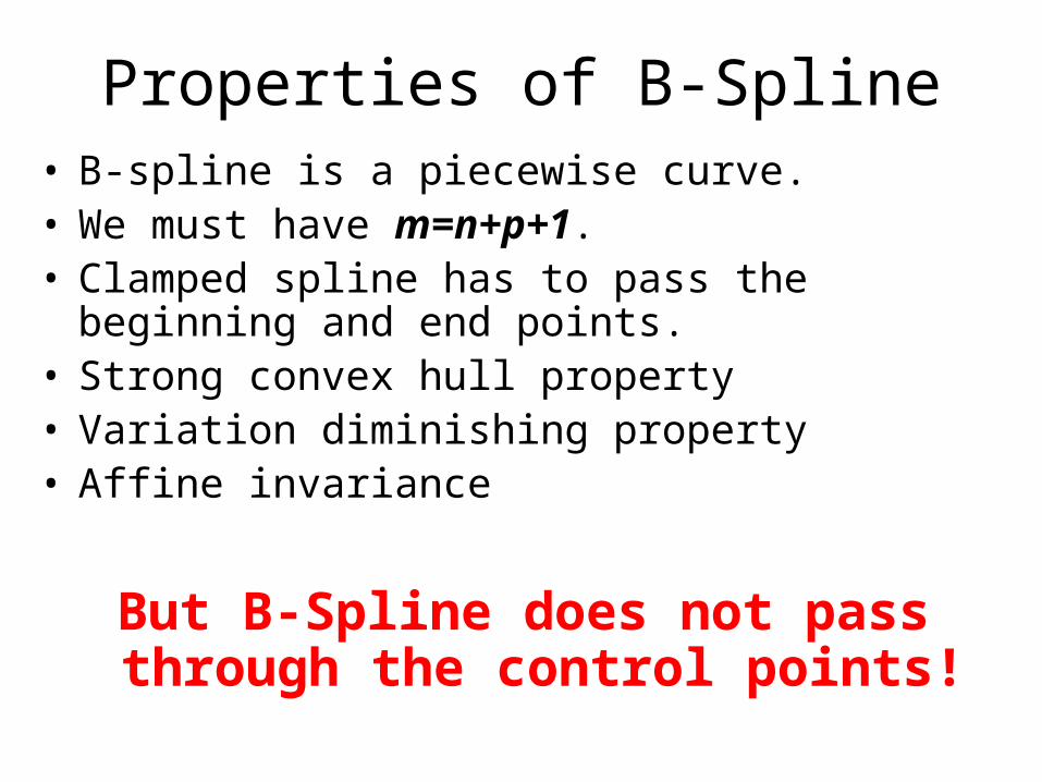
Properties of B-Spline• B-spline is a piecewise curve.• We must have m=n+p+1.• Clamped spline has to pass the beginning and end

points.• Strong convex hull property• Variation diminishing property• Affine invariance

But B-Spline does not pass through the control points!

Variation Diminishing Property:no straight line (resp., plane) intersects a B-spline

curve more times than it intersects the curve's

control polygon.

Summary

• The differences between different splines seems to be huge.

• Based on principles of least interferences and maximum smoothness, we selected natural spline as the base for EMD.

• Different splines (except B-spline) should not change the scales of the IMFs, but it would change the shape and energy levels.

• EMD is unique with respect to all parameters selected.