arX

iv:g

r-qc

/031

1066

v1 2

0 N

ov 2

003

Spin Foam Models

of

Quantum Spacetime

Daniele Oriti

Girton College

Dissertation submitted for the degree of Doctor of Philosophy

University of Cambridge

Faculty of Mathematics

Department of Applied Mathematicsand Theoretical Physics

2003

A Sandra

A Epifaniotto

1

(TALKING TO HIS BRAIN) Ok, brain. Let’s face it. I don’t like you,

and you don’t like me, but let’s get through this thing, and then I can

continue killing you with beer!

Homer J. Simpson

....In formulating any philosophy, the first consideration must always be:

what can we know? That is, what can we be sure we know, or sure that

we know we knew it, if indeed it is at all knowable. Or have we simply

forgotten it and are too embarassed to say anything? Descartes hinted at

the problem when he wrote: “My mind can never know my body, although

it has become quite friendly with my legs.” .....Can we actually “know”

the Universe? My God, it is hard enough to find your way around in

Chinatown! The point, however, is: Is there anything out there? And

why? And must they be so noisy?....

Woody Allen

As far as the laws of mathematics refer to reality, they are not certain,

and as far as they are certian, they do not refer to reality.

Albert Einstein

Those are my principles, and if you don’t like them..well, I have others.

Groucho Marx

Whenever people agree with me, I feel I must be wrong...

Oscar Wilde

2

Contents

1 Introduction 12

1.1 The search for quantum gravity . . . . . . . . . . . . . . . . . . . . . 12

1.2 Conceptual ingredients and motivations . . . . . . . . . . . . . . . . . 14

1.2.1 Background independence and relationality . . . . . . . . . . . 16

1.2.2 Operationality . . . . . . . . . . . . . . . . . . . . . . . . . . . 19

1.2.3 Discreteness . . . . . . . . . . . . . . . . . . . . . . . . . . . . 21

1.2.4 Covariance . . . . . . . . . . . . . . . . . . . . . . . . . . . . . 26

1.2.5 Symmetry . . . . . . . . . . . . . . . . . . . . . . . . . . . . . 34

1.2.6 Causality . . . . . . . . . . . . . . . . . . . . . . . . . . . . . 36

1.3 Approaches to quantum gravity . . . . . . . . . . . . . . . . . . . . . 38

1.3.1 The path integral approach to quantum gravity . . . . . . . . 39

1.3.2 Topological quantum field theories . . . . . . . . . . . . . . . 42

1.3.3 Loop quantum gravity . . . . . . . . . . . . . . . . . . . . . . 44

1.3.4 Simplicial quantum gravity . . . . . . . . . . . . . . . . . . . . 55

1.3.5 Causal sets and quantum causal histories . . . . . . . . . . . . 59

1.4 General structure of spin foam models . . . . . . . . . . . . . . . . . 63

2 Spin foam models for 3-dimensional quantum gravity 72

2.1 3-dimensional gravity as a topological field theory: continuum and discrete cases 73

2.2 Quantum simplicial 3-geometry . . . . . . . . . . . . . . . . . . . . . 76

2.3 The Ponzano-Regge spin foam model: a lattice gauge theory derivation 82

2.4 A spin foam model for Lorentzian 3d quantum gravity . . . . . . . . 85

2.5 Quantum deformation and the Turaev-Viro model . . . . . . . . . . . 88

2.6 Asymptotic values of the 6j-symbols and the connection with simplicial gravity 91

3

2.7 Boundary states and connection with loop quantum gravity: the Ponzano-Regge model as a generalized projector operator 97

2.8 Group field theory formulation and the sum over topologies . . . . . . 102

2.9 Quantum gravity observables in 3d: transition amplitudes . . . . . . 109

3 The Turaev-Viro invariant: some properties 112

3.1 Classical and quantum 3d gravity, Chern-Simons theory and BF theory112

3.2 The Turaev-Viro invariant for closed manifolds . . . . . . . . . . . . . 115

3.3 Evaluation of the Turaev-Viro invariant for different topologies . . . . 117

3.4 The Turaev-Viro invariant for lens spaces . . . . . . . . . . . . . . . . 123

4 Spin foam models for 4-dimensional quantum gravity 130

4.1 4-dimensional gravity as a constrained topological field theory: continuum and discrete cases131

4.2 Quantum 4-dimensional simplicial geometry . . . . . . . . . . . . . . 139

4.3 Discretization and quantum constraints in the generalized BF-type action for gravity149

4.3.1 Generalized BF-type action for gravity . . . . . . . . . . . . . 151

4.3.2 Field content and relationship with the Plebanski action . . . 156

4.3.3 Spin foam quantization and constraints on the representations 160

4.3.4 Alternative: the Reisenberger model . . . . . . . . . . . . . . 163

4.3.5 The role of the Immirzi parameter in spin foam models . . . . 167

4.4 A lattice gauge theory derivation of the Barrett-Crane spin foam model170

4.4.1 Constraining of the BF theory and the state sum for a single 4-simplex170

4.4.2 Gluing 4-simplices and the state sum for a general manifold with boundary180

4.4.3 Generalization to the case of arbitrary number of dimensions . 185

4.5 Derivation with different boundary conditions and possible variations of the procedure188

4.5.1 Fixing the boundary metric . . . . . . . . . . . . . . . . . . . 189

4.5.2 Exploring alternatives . . . . . . . . . . . . . . . . . . . . . . 192

4.6 Lattice gauge theory discretization and quantization of the Plebanski action198

4.7 The Lorentzian Barrett-Crane spin foam model: classical and quantum geometry200

4.7.1 Geometric meaning of the variables of the model . . . . . . . . 203

4.7.2 Simplicial classical theory underlying the model . . . . . . . . 207

4.7.3 Quantum geometry: quantum states on the boundaries and quantum amplitudes209

4.7.4 The Barrett-Crane model as a realization of the projector operator215

4.8 Asymptotics of the 10j-symbol and connection with the Regge action 220

4

5 The group field theory formulation of spin foam models in 4d 224

5.1 General formalism . . . . . . . . . . . . . . . . . . . . . . . . . . . . 226

5.2 Riemannian group field theories . . . . . . . . . . . . . . . . . . . . . 232

5.2.1 The Perez-Rovelli version of the Riemannian Barrett-Crane model232

5.2.2 The DePietri-Freidel-Krasnov-Rovelli version of the Barrett-Crane model235

5.2.3 Convergence properties and spin dominance . . . . . . . . . . 237

5.2.4 Generalized group field theory action . . . . . . . . . . . . . . 240

5.3 Lorentzian group field theories . . . . . . . . . . . . . . . . . . . . . . 246

5.4 Quantum field theoretic observables: quantum gravity transition amplitudes250

5.5 A quantum field theory of simplicial geometry? . . . . . . . . . . . . 254

6 An orientation dependent model: implementing causality 259

6.1 A causal amplitude for the Barrett-Crane model . . . . . . . . . . . . 260

6.1.1 Lorentzian simplicial geometry . . . . . . . . . . . . . . . . . . 260

6.1.2 Stationary point analysis and consistency conditions on the orientation262

6.1.3 A causal transition amplitude . . . . . . . . . . . . . . . . . . 264

6.2 Barrett-Crane model as a quantum causal set model . . . . . . . . . . 270

7 The coupling of matter and gauge fields to quantum gravity in spin foam models281

7.1 Strings as evolving spin networks . . . . . . . . . . . . . . . . . . . . 282

7.2 Topological hypergravity . . . . . . . . . . . . . . . . . . . . . . . . . 285

7.3 Matter coupling in the group field theory approach . . . . . . . . . . 287

7.4 A spin foam model for Yang-Mills theory coupled to quantum gravity 291

7.4.1 Discretized pure Yang–Mills theory . . . . . . . . . . . . . . . 293

7.4.2 The coupled model . . . . . . . . . . . . . . . . . . . . . . . . 295

7.4.3 The coupled model as a spin foam model . . . . . . . . . . . . 299

7.4.4 Features of the model . . . . . . . . . . . . . . . . . . . . . . . 301

7.4.5 Interplay of quantum gravity and gauge fields from a spin foam perspective302

8 Conclusions and perspectives 306

8.1 Conclusions... . . . . . . . . . . . . . . . . . . . . . . . . . . . . . . . 306

8.2 ...and perspectives . . . . . . . . . . . . . . . . . . . . . . . . . . . . 309

5

Declaration

This dissertation is based on research done at the Department of Applied Mathemat-

ics and Theoretical Physics at the University of Cambridge between January 2000

and June 2003. No part of it or anything substantially the same has been previously

submitted for a degree or any other qualification at this or at any other University.

It is the result of my own work and includes nothing which is the outcome of work

done in collaboration, except where specifically indicated in the text. Section 4.4

contains work done in collaboration with R. M. Williams. Section 4.3, section 4.7,

and Chapter 6 contain work done in collaboration with E. R. Livine. Section 7.4

contains work done in collaboration with H. Pfeiffer. Section 5.2.4 and section 5.5

describe work in progress and to be published. This thesis contains material which

has appeared on the electronic print archive http://arXiv.org, and which has been

published in the following papers:

1. Daniele Oriti, Ruth MWilliams, Gluing 4-simplices: a derivation of the Barrett-

Crane spin foam model for Euclidean quantum gravity, Phys.Rev. D 63 (2001)

024022; gr-qc/0010031;

2. Etera R. Livine, Daniele Oriti, Barrett-Crane spin foam model from a general-

ized BF-type action for gravity, Phys. Rev. D65, 044025 (2002); gr-qc/0104043;

3. D. Oriti, Spacetime geometry from algebra: spin foam models for non-perturbative

quantum gravity, Rep. Prog. Phys. 64, 1489 (2001); gr-qc/0106091;

4. D. Oriti, Boundary terms in the Barrett-Crane spin foam model and consistent

gluing, Phys. Lett. B 532, 363 (2002); gr-qc/0201077;

6

5. D. Oriti, H. Pfeiffer, A spin foam model for pure gauge theory coupled to

quantum gravity, Phys. Rev. D 66, 124010 (2002); gr-qc/0207041;

6. E. R. Livine, D. Oriti, Implementing causality in the spin foam quantum ge-

ometry, Nucl. Phys. B 663, 231 (2003); gr-qc/0210064;

7. E. R. Livine, D. Oriti, Causality in spin foam models for quantum gravity, to

appear in the Proceedings of the XV SIGRAV Conference on General Rela-

tivity and gravitational physics (2003); gr-qc/0302018;

7

Acknowledgements

There are so many people I would like to thank for having made this work possible.

Acknowledging them all would take too long....and it will!

I am deeply grateful to my supervisor, Dr. Ruth M. Williams, for her uncondi-

tional support and help, both at the scientific and non-scientific level, for the many

discussions, for her kindness, and for always being such a wonderful person with me.

Thanks, Ruth!

A special thank goes to Etera Richard Livine, for being at the same time a great

collaborator to work with and a wonderful friend to have fun with. It’s amazing we

managed somehow to do some work while having fun! Thanks!

Most of what I know about the subject of this thesis I’ve learnt from conversations

and discussions with other people, that helped me to shape my ideas, to understand

more, and to realize how much I still have to understand and to improve. To name

but a few: John Baez, John Barrett, Olaf Dreyer, Laurent Freidel, Florian Girelli,

Etera Livine, Renate Loll, Fotini Markopoulou, Robert Oeckl, Hendryk Pfeiffer,

Mike Reisenberger, Carlo Rovelli, Hanno Sahlmann, Lee Smolin, Ruth Williams.

To all of you (and the others I didn’t mention), thanks for your help and for always

being so nice! You reminded me continously of how many great guys are out there!

Of course, the stimulating atmosphere of DAMTP has greatly helped me during

the course of this work, so thanks to all the DAMTP people, faculty, staff, students

and postdocs, for making it such a great place to work in.

Also, the work reported in this thesis would have not been possibly carried out

without the financial support coming from many different sources, covering my fees,

my mantainance, and expenses for travel and conferences, that I gratefully acknowl-

edge: Girton College, the Engineering and Physical Sciences Research Council, the

8

Cambridge European Trust, the Cambridge Philosophical Society, Trinity College,

the Isaac Newton Trust and the C.T. Taylor Fund.

Now it is time to thank all those who have indirectly improven this work, by

improving my personal life, contributing greatly to my happiness, making me a

better person, helping me when I needed it and teaching me so much.

I would like to thank very much all my friends in Cambridge, who have made the

last three years there so enjoyable, for the gift of their friendship; with no presump-

tion of completeness, thanks to: Akihiro Ishibashi, Christian Stahn, David Mota

and Elisabeth, Erica Zavala Carrasco, Francesca Marchetti, Francis Dolan, Gio-

vanni Miniutti, Joao Baptista, Joao Lopez Dias, Martin Landriau, Matyas Karadi,

Mike Pickles, Mohammed Akbar, Petra Scudo, Raf Guedens, Ruben Portugues, Sig-

bjorn Hervik, Susha Parameswaran, Tibra Ali, Toby Wiseman and Yves Gaspar.

You are what I like most in Cambridge!

I am grateful to my family, for their full support and encouragement, during

the last three years just as much as during all my life. So, thanks to my father

Sebastiano and my mother Rosalia, who have been always great in the difficult job

of being my parents, vi voglio bene! Thanks to my sister Angela, because one could

not hope for a better sister! Sono orgoglioso di te! And thanks to Epi, who has

been, with his sweetness and love, the best non-human little brother one could have.

Mi manchi, Epifaniotto!

I cannot thank enough all my friends in Rome and in Italy, for what they gave me

by just being my friends and for the happiness this brings into my life; being sorry

for surely neglecting someone: Alessandra, Andrea, Antonio, Carlo, Cecilia, Chiara,

Claudia, Daniela, Daniele C., Daniele M., David, Davide, Federico, Gianluca M.,

Gianluca R., Giovanni, Luisa, Marco, Matteo, Nando, Oriele, Pierpaolo, Roberto,

Sergio, Silvia, Simone E., Simone S., Stefano. I feel so lucky to have you all! Vi

voglio bene, ragazzi!

Finally, Sandra; I thank you so much for being what you are, for making me

happy just by looking at you and thinking of you, for being always so close and

lovely, for making me feel lucky of having you, for sharing each moment of my life

with me, and for letting me sharing yours; for all this, and all that I am not able to

say in words, thanks. Sei tutto, amore!

9

Summary

Spin foam models are a new approach to the construction of a quantum theory of

gravity. They aim to represent a formulation of quantum gravity which is fully

background independent and non-perturbative, in that they do not rely on any

pre-existing fixed geometric structure, and covariant, in the spirit of path integral

formulations of quantum field theory.

Many different approaches converged recently to this new framework: loop quan-

tum gravity, topological field theory, lattice gauge theory, path integral or sum-over-

histories quantum gravity, causal sets, Regge calculus, to name but a few.

On the one hand spin foam models may be seen as a covariant (no 3+1 splitting)

formulation of loop quantum gravity, on the other hand they are a kind of transla-

tion in purely algebraic and combinatorial terms of the path integral approach to

quantum gravity.

States of the gravitational field, i.e. possible 3-geometries, are represented by

spin networks, graphs whose edges are labelled with representations of some given

group, while their histories, i.e. possible (spacetime) 4-geometries, are spin foams,

2-complexes with faces labelled by representations of the same group. The models

are then characterized by an assignment of probability amplitudes to each element

of these 2-complexes and are defined by a sum over histories of the gravitational

field interpolating between given states. This sum over spin foams defines the par-

tition function of the theory, by means of which it is possible to compute transition

amplitudes between states, expectation values of observbles, and so on.

In this thesis we describe in details the general ideas and formalism of spin

foam models, and review many of the results obtained recently in this approach.

We concentrate, for the case of 3-dimensional quantum gravity, on the Turaev-Viro

10

model, and, in the 4-dimensional case, which is our main concern, on the Barrett-

Crane model, based on a simplicial formulation of gravity, and on the Lorentz group

as symmetry group, both in its Riemannian and Lorentzian formulations, which is

currently the most promising model among the proposed ones.

For the Turaev-Viro model, we show how it gives a complete formulation of

3-dimensional gravity, discuss its space of quantum states, showing also the link

with the loop quantum gravity approach, and that with simplicial formulations of

gravity, and finally give a few example of the evaluation of the partition function

for interesting topologies.

For the Barrett-Crane model, we first describe the general ideas behind its con-

struction, and review what it is known up to date about this model, and then

discuss in details its links with the classical formulations of gravity as constrained

topological field theory.

We show a derivation of the model from a lattice gauge theory perspective,

in the general case of manifold with boundaries, discussing the issue of boundary

terms in the model, showing how all the different amplitudes for the elements of the

triangulations arise, and presenting also a few possible variations of the procedure

used, discussing the problems they present.

We also describe how, from the same perspective, a spin foam model that couples

quantum gravity to any gauge theory may be constructed, and its consequences for

our understanding of both gravity and gauge theory.

We analyse in details the classical and quantum geometry of the Barrett-Crane

model, the meaning of the variables it uses, the properties of its space of quantum

states, how it defines physical transition amplitudes between these states, the classi-

cal formualtions of simplicial gravity it corresponds to, all its symmetry properties.

Then we deal with the issue of causality in spin foam models in general and in the

Barrett-Crane one in particular. We describe a general scheme for causal spin foam

models, and the resulting link with the causal set approach to quantum gravity. We

show how the Barrett-Crane model can be modified to implement causality and to

fit in such a scheme, and analyse the properties of the modified model.

11

Chapter 1

Introduction

1.1 The search for quantum gravity

The construction of a quantum theory of gravity remains probably the issue left

unsolved in theoretical physics in the last century, in spite of a lot of efforts and many

important results obtained during an indeed long history of works (for an account

of this history see [1]). The problem of a complete formulation of quantum gravity

is still quite far from being solved (for reviews of the present situation see [2, 3, 4]),

but we can say that the last (roughly) fifteen years have seen a considerable number

of developments, principally identifiable with the construction of superstring theory

[5, 6], in its perturbative formulation and, more recently, with the understanding of

some of its non-perturbative features, with the birth of non-commutative geometry

[7, 8, 9], and with the renaissance of the canonical quantization program in the form

of loop quantum gravity [10, 11], based on the reformulation of classical General

Relativity in terms of the Ashtekar variables [12]. In recent years many different

approaches on the non-perturbative and background-independent side have been

converging to the formalism of the so-called spin foams [13, 14, 15], and this class

of models in the subject of this thesis.

Why do we want to quantize gravity? There are many reasons for this[17]: the

presence of singularities in classical General Relativity [18], showing that something

in this theory goes wrong when we try to use it to describe spacetime on very small

scales; the fact that the most general form of mechanics we have at our disposal in

12

describing Nature is quantum mechanics and that this is indeed the language that

proved itself correct in order to account for the features of the other three fundamen-

tal interactions, so that one is lead to think that the gravitational interaction too

must be described within the same conceptual and semantic framework; the desire

to unify all these interactions, i.e. to find a unified theory that explains all of them

as different manifestation of the same physical entity; the ultraviolet divergences

one encounters in quantum field theory, that may be suspected to arise because at

high energies and small scales the gravitational interaction should be necessarily

taken into account; the necessity for a theory describing the microscopic degrees

of freedom responsible for the existence of an entropy associated with black holes

[19, 20] and more generally with any causal horizon [21]; more generally, the need

to explain the statistical mechanics behind black hole thermodynamics; the need

to have a coherent theory describing the interaction of quantum gauge and matter

fields with the gravitational field, beyond the approximation of quantum field theory

in curved spaces; the unsolved issues in cosmology asking for a more fundamental

theory to describe the origin of our universe, at energies and distances close to the

Planck scale.

The reader may add her own preferred reasons, from a physical or mathematical

point of view, but what remains in our opinion the most compelling one is the

purely conceptual (philosophical) one, well explained in [22, 23], given by the need

to bring together the two conceptual revolutions with which the last century in

physics started, represented by General Relativity and Quantum Mechanics. The

main elements of these two paradigmatic shifts (in Kuhn’s sense) of our picture

of the natural world can be summarised, we think, as: 1) spacetime is nothing

other than the gravitational field, and that it is a dynamical entity and not a fixed

background stucture on which the other fields live; consequently, any determination

of localization has to be fully relational, since no fixed structure exists that can be

used to define it in an absolute way; 2) all dynamical objects, i.e. all dynamical fields,

are quantum objects, in the sense of having to be described within the framework

of quantum mechanics, whatever formalism for quantum mechanics one decides to

use (operators on Hilbert spaces, consistent histories, etc.).

This requires a peculiar (and, admittedly, conceptually puzzling) relationship

between observed systems and observers, and it is best characterized by a relational

13

point of view that assigns properties to physical systems only relative to a given

observer, or that deals with the information that a given observer has about a given

physical system, and that because of this favours an operational description of all

physical systems.

The problem we face, from this perspective, is then to give a more fundamental

description of spacetime and of its geometry than that obtained from General Rela-

tivity, to construct a more fundamental picture of what spacetime is, to understand

it as a quantum entity, to grasp more of the nature of space and time.

Before getting to the particular approach to the construction of a quantum theory

of gravity represented by spin foam models, we think it is useful to account for the

main ideas and motivations, that in one way or another are at the roots of this

approach, in order to understand better what is, in our opinion, the conceptual

basis of the spin foam approach, as it is presently understood (by us).

1.2 Conceptual ingredients and motivations

Let us list what we think are the conceptual ingredients that should enter in a

complete formulation of a theory of quantum gravity, mostly coming from insights

we obtain from the existing theory of the gravitational field, General Relativity, and

from the framework of quantum mechanics, and partly resulting from independent

thinking and intuitions of some of the leaders of quantum gravity research.

The list is as follows: a theory of quantum gravity should be background

independent and fully relational, it should reveal a fundamental discreteness

of spacetime, and be formulated in a covariant manner, with the basic objects

appearing in it having a clear operational significance and a basic role played by

symmetry principles, and a notion of causality built in at its basis.

By background independence and relationality we mean that the physical signif-

icance of (active) diffeomorphism invariance of General Relativity has to be man-

tained at the quantum level, i.e there should be no room in the theory for any fixed,

absolute background spacetime structure, for any non-dynamical object, that any

physical quantity has to be defined with respect to one or more of the dynamical

objects the theory deals with, and also the location of such objects has to be so

14

defined.

A fundamental discreteness of spacetime at the Planck scale is to be expected for

many reasons, included the way quantum mechanics describes states of systems in

terms of a finite set of quantum numbers, the ultraviolet divergences in QFT and the

singularities in GR, both possibly cured by a fundamental cut-off at the Planck scale,

and the finiteness of black hole entropy, also possibly explained by such a minimal

length (the entropy of a black hole would be infinite if infinitesimal fluctuations of

both graitational and matter degrees of freedom were allowed at the horizon [20]),

not mentioning hints coming from successes and failures of several approaches to

quantum gravity pursued in the long history of the subject, including the discrete

spectrum for geometric operators obtained in the context of loop quantum gravity

(showing also a minimal quantum of geometry of the order of the Planck length),

and the difficulties in giving meaning to the path integral for quantum gravity in a

continuum formulation.

A covariant formulation, treating space and time on equal footing, is also to be

preferred both in the light of how space and time are treated in General Relativity

and of the fact that such a covariant formulation can be shown to be the most general

formulation for a mechanical theory, both at the classical and quantum level, as we

are going to discuss.

Operationality would imply the quantities (states and observables) appearing

in the formulation of the theory to have as clear-cut a physical interpretation as

possible, to be related easily to operations one can perform concretely and not to

refer to abstract ontological entities away from experimental (although maybe ideal-

ized) verification; such operationality, however appealing on philosophical grounds,

is even more necessary in a quantum mechanical setting, where the observables are

not only needed to interpret the theory but also for its very definition.

Also, the use of symmetries to characterize physical systems has a long and

glorious history, so does not need probably too much justification, but in this case

it is doubly relevant: on the one hand, operationality applied to spacetime would

suggest the use of symmetry transformations on spacetime objects to play a key role

in defining the observables and the states of the theory (also recalling that it is the

parallel transport of objects along suitable paths that indicates the presence of a non-

trivial geometry of spacetime); on the other hand, the impossibilty of using geometric

15

structures as starting point, since they have to emerge from more fundamental non-

geometric ones, suggests that the proper language to be used in quantum gravity

is algebraic, and coming from the algebraic context of the representation theory of

some symmetry group.

As for causality, first of all it is a fundamental component of our understanding

of the world, so its presence at some level of the theory is basically compulsory,

second, it is very difficult to envisage a way in which it can emerge as the usual

spacetime causal structure if not already present at least in some primitive form at

the fundamental level.

Let us analyse all these ideas in more detail.

1.2.1 Background independence and relationality

The gauge invariance of General Relativity, i.e. diffeomorphism invariance, requires

the absence of any absolute, non-dynamical object in the theory [24]; the spacetime

background itself, spacetime geometry, has to be dynamical and not fixed a priori;

therefore no statement in the theory can refer to a fixed background, but has to

be fully relational in character, expressing a correlation between dynamical vari-

ables; this is what is meant by background independence, a necessary requirement

for any complete theory of quantum gravity, also because it is already present in

classical GR. In practice, this fact translates into the requirements that observables

in gravity have to be diffeomorphism invariant, i.e. gauge invariant as in any gauge

theory, so cannot depend on spacetime points[25]; in a canonical formulation they

have to commute with the gravity constraints, both at the classical and quantum

level; therefore they have to be either global, e.g. the volume of the universe, or

local if locality is defined in terms of the dynamical quantities of the theory, e.g.

some geometrical quantity at the event where some metric component has a given

value, or, if some matter field is considered, some geometrical quantity where the

matter field has a certain value[25]. In any case, any local observable will define

some correlation between the dynamical fields (more generally, between the partial

observables of the theory [26]) which are present, and must therefore take into ac-

count the equaton of motion of these fields. This has to be true both at the classical

and quantum level.

16

This has important consequences also for the interpretation of quantum gravity

states. The only physically meaningful definition of locality in GR is relational,

as we said. Once quantized, the metric field, spacetime, has to be described (in

one formulation of quantum theory) in terms of states in a Hilbert space; however,

because of the mentioned relationality of the concept of localization, the states of

the gravitational field cannot describe excitations of a field localized somewhere on

some background space, but must describe excitations of spacetime itself, being thus

defined regardless of any background manifold[22].

One can push this idea even further and say that, at a fundamental level, be-

cause of diffeomorphism invariance, there should not be any spacetime at all, in the

sense that no set of spacetime points, no background manifold, should exist, with

a spacetime point being defined by where a given field is, or, better, that we ought

to reconstruct a notion of spacetime and of spacetime events from the background

independent gravitational quantum states, from the quanta of spacetime, because

of the identification between the gravitational field and spacetime geometry.

The idea would then be that they are (linear combinations of) eigenstates of

geometric operators, such as lengths, areas and volumes, although they must be

given in terms of non-geometric diffeomorphism invariant informations, in order to

make sense regardless of any spacetime manifold and to be able to reconstruct such

a manifold from them, including its geometry; therefore they are non-local, in the

sense of not being localized anywhere in a background manifold, they are instead

the “where” with respect to which other fields may be localized. If not geometric,

the ingredients coming into their definition have to be purely combinatorial and

algebraic; they are like “seeds” of space, “producing” it by suitable translation of

non-geometric into geometric information; in the same sense their dynamics should

also be given in purely algebraic and combinatorial terms, expressed by the definition

of transition amplitudes between quantum gravity states only, either expressed as

canonical inner products or as sum-over-histories, and should not take place “in

time” but rather define what time is, for other gauge or matter fields; therefore, these

transition amplitudes will not depend on any time variable at all, not a coordinate

time, not a proper time, no time variable at all. Of course this does not mean

that they do not contain any notion of time, but only that this notion is not of the

familiar classical form [27]. We will later see how these ideas are realized in practice

17

in loop quantum gravity and spin foam models.

Let us briefly note that the relational point of view forced on us by GR is somehow

reminescent of the ideas at the roots of category theory, where indeed objects are

treated on the same footing as relationships between objects, and in a sense what

really matters about objects is indeed only their relationships with other objects;

the importance of category theory in quantum gravity is suggested by the way 3-

d gravity can indeed be quantized by categorical methods and expressed nicely in

categorical terms, as we will discuss. It has in fact been repeatedly argued that

the general framework of topological field theory can be adapted to 4-dimensional

quantum gravity, implying that the right formulation of 4-d quantum gravity has to

be in categorical terms; also this is partly realized in spin foam models [28]. This

is a way in which algebra, in this case, categorical algebra, can furnish the more

fundamental language in which to describe spacetime geometry [29].

If taken seriously, background independence has important implications for the

fomulations of the theory; for example, the absence of a fixed background structure

implies that the theory must be formulated in a non-perturbative fashion, from the

metric point of view, in order to be considered truly fundamental, and to incorporate

satisfactorily the symmetries of the classical theory.

This means that it cannot be formulated by fixing a metric, or its corresponding

quantum state, and then only considering the perturbations around it, although

of course this is an approximation that we should be able to use in some limited

context, since it describes, for example, the situation we live in. Of course this does

not mean that no perturbative expansion at all can be used in the formulation of the

theory, but only that, if used, each term in such a perturbation expansion should be

defined in a background independent way. We will see an explicit example of this

in the group field theory formulation of spin foam models.

A simple system to study, which nevertheless presents many analogies with the

case of General Relativity, is that represented by a relativistic particle in Minkowski

space, since it may be thought of as something like “General Relativity in 0 spatial

dimensions”. Its configuartion variables are the spacetime coordinates xµ and its

18

classical action is:

S(x) =

λ2∫

λ1

(−m)

√

dxµ

dλ

dxµdλ

dλ. (1.1)

The system is invariant under reparametrization λ → f(λ) of the trajectory of the

particle, and this is analogous to a time diffeomorphism in General Relativity (this

is the sense in which one may think of this elementary system as similar to General

Relativity in 0 spatial dimensions) that reduce to the identity on the boundary. It

is often convenient to pass to the Hamiltonian formalism. The action becomes:

S(x) =

λ2∫

λ1

(pµxµ − N H) dλ (1.2)

where pµ is the momentum conjugate to xµ and H = pµpµ +m2 = 0 (we are using

here the signature (−+++)) is the Hamiltonian constraint that gives the dynamics

of the system (it represents the equation of motion obtained by extremizing the

action above with respect to the variables x, p, and N).

1.2.2 Operationality

Operationality when applied to the construction of a quantum gravity theory would

require the use of fundamental variables with as direct as possible an experimental

meaning, constructed or obtained by performing possibly idealized operations with

clocks, rods, gyroscopes or the like, or requires us to intepret such variables (and

any object in the theory) as a convenient summary of some set of operations we

may have performed[30]. In particular it is the set of observables that has to be

given a clear operational significance, in order to clarify the physical meaning of the

theory itself. Indeed we will see later how the most natural observables (physical

predictions) of classical gravity, these being “classical spin network”, are of a clear

operational significance and directly related to transformations we may perform on

spacetime[31]. This can moreover be translated into the quantum domain more or

less directly, as we shall see.

If the (operational) definition of the observables of the theory is important in

classical mechanics, in order to provide it with physical meaning, it is absolutely

19

crucial in quantum mechanics since it is part of the very definition of the theory.

Indeed, a quantum mechanical theory is defined by a space of states and by a set

of (hermitian) operators representing the observables of the theory [221, 33, 34].

To stress even more the importance of observations and observables in quantum

theory, just note that the states of a system (vectors in a Hilbert space) can be

thought of either as results of a given measurement, if they are eigestates of a given

operator, or as a summary of possible measurements to be performed on the system,

when they are just linear combinations of eigenstates of a given observables (and

this is the general case). Also, the observation (measurement) process is one of the

two dynamical laws governing the evolution of the states of the system considered,

formalized as the collapse of the wave function, with all the interesting and puzzling

features this involves. From a more general perspective, quantum mechanics is about

observations that some subsystem of the universe (observer) makes of some other

(observed) system, and one can push this point of view further to state that the

very notion of state of a given system is necessarily to be considered as relative to

some observer in order to make sense, and as just a collection of possible results

of her potential measurements (observations)[32]; This point of view has interesting

connections with (quantum) information theory, in which context it is in some sense

the natural point of view on quantum mechanics [34, 35]; also, it is natural in the

context of topological field theory (of which 3-dimensional quantum gravity is an

important example), and can be phrased, related to these, in categorical language

[29, 266].

In a sense, thus, quantum mechanics is operational from the very onset, and can

be made even more “operational-looking” if one formulates it in such a way that

it reflects more closely what are the conditins and the outcomes of realistic mea-

surements and observations[36]. Such a reformulation [37] uses spacetime smeared

states and a covariant formulation of both classical and quantum mechanics, where

the basic idea is to treat space and time on equal footing. It is apparent that such a

formulation is more naturally adapted to a quantum gravity context than the usual

one based on a rigid splitting between a space manifold and a fixed time coordi-

nate. We will describe such a formulation in more detail when discussing the issue

of covariance.

20

1.2.3 Discreteness

As we said above, there are many reasons to question the correctness of the usual

assumption that spacetime has to be represented by a smooth manifold, and to

doubt the physical meaning of the very concept of a spacetime “point”[38]. So, is

spacetime a C∞-manifold? What is the meaning of a spacetime point? Is the very

idea and use of points justified from the general relativistic and quantum mechanical

perspective? If not, then what replaces it?

In both canonical loop quantum gravity and path integral approaches a con-

tinuum differentiable manifold is assumed as a starting point (even if in the path

integral approach one then treats the topology of the manifold as a quantum vari-

able to be summed over), but then in the loop approach the development of the

theory itself leads beyond the continuum, since the states of the theory (at least in

one (loop) representation) are non-local, combinatorial and algebraic only, and the

spectrum of the geometric operators is discrete. One may instead take the point of

view that the continuum is only a phenomenological approximation, holding away

from the Planck scale, or in other words when the resolution of our measurements

of spacetime is not good enough; therefore a continuum manifold is what we may

use to represent spacetime only if we do not test it too closely, and only if we do

not need any precise description of it. One may also say that the continuum has no

operational meaning, or that it is the result of an idealization in which our sensitiv-

ity is assumed to be infinite, in the same sense as classical mechanics results from

quantum mechanics in the ideal limit in which our intervention does not influence

the system under observation (Planck’s constant going to zero), so that a continuum

decsription cannot hold at a fundamental level. From the operational point of view,

spacetime is modeled and should be modeled by what our observations can tell us

about it, and because these are necessarily of finite resolution then spacetime cannot

be modeled by a set of point with the cardinality of the continuum.

What description should we look for, then? One may take the drastic attitude

that the ultimate theory of spacetime should not be based on any concept of space-

time at all, and that only some coarse graining procedure will lead us, in several

steps, to an approximation where the concept of a “local region” does indeed make

sense, but not as a subset of a “spacetime”, but as an emergent concept, and where

21

a collection of such regions can be defined and then interpreted as the collection of

open coverings of a continuum manifold. In this way it would be just like there exists

some continuum manifold representing spacetime, to which our collection of local

regions is an approximation, although no continuum manifold plays any role in the

formulation of the fundamental theory, so that the collection of local regions, if not

truly fundamental, is definitely “more fundamental” than the continuum manifold

itself. Of course, if the physical question one is posing allows for it, one may at this

point use the emerging continuum manifold as a description of spacetime and use

the theory in this approximation. It may also be, if one does not subscribe to any

realistic point of view for scientific theories, that there is no real meaning to the

idea of a “fundamental theory”, but also in this case, the description of spacetime in

terms of collections of local regions as opposed to that using a continuum manifold

seems to be more reasonable, also in light of the operational point of view mentioned

above[38]1.

If a continuum description of spacetime is not available at a fundamental level,

either because we are forced by the theory itself to take into account the not infinite

precision of our measurements, or because there exists a minimum length that works

as a least bound for any geometric measurement, as implied by SU(2) loop quantum

gravity, and hinted at from many different points of view, or because simply we want

to avoid the idealization of a spacetime point, then we are forced to consider what

kind of discrete substratum may replace the usual smooth manifold. The continuum

may be regarded as a fundamentally problematic idealization in that it involves an

infinite number of elements also requiring an infinite amount of information to be

distinguished from each other, so we want to look for some substitute of it in the form

of a topological space (in order to remain as close as possible to the approximation

we want to recover) in which any bounded region contains only a finite number

of elements, i.e. we would work with a “finitary” topological space[39, 40]. The

collection of local regions mentioned above would be in fact a space of this sort.

Of course, a necessary condition for a finitary topological space to be sensibly used

as a substitute for a continuum spacetime manifold is that the former does indeed

1It is maybe interesting to note that, even in the continuum case, a topology of a space M is

indeed defined as the family of open subsets of M .

22

approximate in a clear sense the latter, and that a limit can be defined in which this

approximation does indeed become more and more precise.

Let us be a bit more precise. Given a topological space S, from the operational

point of view the closest thing to a point-event we can possibly measure is an open

subset of S, and it is important to note that the definiton of the topology of S is

exactly given by a family of open subsets of S, so that to have access to only a finite

number of open sets means to have access to a subtopology U of S. Operationally

then, our knowledge about the topology of S can be summarized in the space F (U)

obtained by identifying with each other any point of S that we cannot be distin-

guished by the open sets in U . Therefore, given the open cover U of S, assumed to

form a subtopology of S, i.e. to be finite and closed under union and intersection,

we regard x, y ∈ S as equivalent if and only if ∀u ∈ U, x ∈ U ⇔ y ∈ U . Then

F (U) is the quotient of S with respect to this equivalence relation. Another way to

characterize the space F (U) is considering it as the T0-quotient of S with respect

to the topology U2. If one considers F (U) as an “approximation” to a topological

space S, one can show that such approximation becomes exact as more and more

open sets are used, i.e. as the open covering is refined. Of course, without such

a result, it would be impossible to claim that finitary topological spaces or posets

represent a more fundamental substratum for a continuum spacetime[39].

We note that a finitary topological space has an equivalent description as a

poset, i.e. a partially ordered set; in fact the collection C of subsets of the set

F is closed under union and intersection, and consequently one can define for any

x ∈ F a smallest neighborhood Λ(x) = ∩A ∈ C|x ∈ A. Because of this the

natural ordering of subsets translates into a relation among the elements of F :

x→ y ⇔ Λ(x) ⊂ Λ(y) ⇔ x ∈ Λ(y). This relation is reflexive (x→ x) and transitive

(x → y → z ⇒ x → z). On the other hand, one can proceed the other way round,

because any relation between elements of F which satisfies these properties gives

a topology, by defining for any x ∈ F , Λ(x) ≡ y ∈ F |y → x, and defining a

subset A ⊂ F to be open if and only if x → y ∈ A ⇒ x ∈ A. Moreover, such a

relation defines a topology that makes F a T0 space iff no circular order relation

2A space is a T0-space if for any pair of its points there is an open set containing one but not

the other of the two

23

(x → y → x) ever occurs. This means that (F,C) is a T0 space if and only if F is

a partially ordered set (poset). This characterization of a finitary space as a poset

is useful to make a link to the causal set approach we will discuss in the following

[30, 39].

Another very important (although well known) equivalent characterization of a

finitary space such as that represented by an open covering of a given manifold is in

terms of simplicial complexes. Indeed from any open covering one can construct a

simplicial complex by considering the so-called “nerve” of the covering, which is the

simplicial complex having as vertices the open sets of the open covering, and as sim-

plices the finite families of open sets of it whose intersection is non-empty. Therefore

we clearly see how all models that one may construct for quantum gravity, which

are based on the use of simplicial complexes as substitutes for a continuum space-

time, are just applications of this idea of replacing a smooth manifold with a finitary

substitute, and are thus not a technically useful approximation, but on the contrary

more close to a fundamental description of spacetime[40], at least if one accepts the

point of view we are advocating here. In other words, simplicial gravity[41, 42], e.g.

in the Regge calculus formulation[44], represents such a finitary model for gravity

with on top of it a certain operational flavor, with finitary patches of flat space

replacing the spacetime continuum manifold, thus realising at the same time both

this finitary philosophy and the equivalence principle. One can imagine each 4-

simplex to represent something like an imperfect determination of localization[30],

thus replacing the over-idealized concept of a spacetime point, so that the simplicial

complex used in place of the continuum manifold has to be intepreted as the probing

of spacetime by a number of imperfect thus real measurements, or in other words,

the finitary topological space represented by the simplicial complex is the spacetime

we reconstruct from our set of measurements. In this case, the simplicial complex

we use is not the nerve of the open covering mentioned above, but equivalently the

open covering itself; of course, one can then go to the simplicial complex dual to

the original one, and this is precisely the nerve of the simplicial open covering; this

is the dual complex used in spin foam models, which is then seen as also arising

naturally from this operational perspective3.

3Note that the Regge Calculus action itself can be defined on a simplicial complex even if the

24

It is very important to note that the structures of open coverings, nerves, sim-

plicial complexes associated to a space make perfect sense even when such a space

does not consist of points nor is it anything like a continuum manifold, and are

thus much more general than this. Both manifolds and non-manifold spaces give

rise to the same kind of open coverings and simplicial complexes, and both are re-

trieved in the limit of finer coverings. Therefore the difference between manifolds

and non-manifold spaces cannot be seen from the open coverings alone, but must

lie in the relationship between different open coverings, i.e. in the refining maps. It

is the refinement procedure that gives us either a manifold or a non-manifold struc-

ture, depending on how it is defined and performed, and these subtleties must be

taken into account when considering a refinement of a simplicial or finitary model

for quantum gravity associated to a classical limit[40].

In any case, from an operational perspective, the triangulated structure, the

open covering, the simplicial complex, all these structure are not to be thought of as

imposed on the manifold, or as approximations of it, but are the result of the process

of “observing” it, they are a representation of a set of observations of spacetime. This

change in perspective should affect the way certain issues are faced, like for example

the issue of “triangulation independence” or the way a sum over triangulations or

2-complexes is dealt with (should one take the number of vertices to infinity? what

are diffeomorphisms from this point of view? what if the underlying space we try

to recover is not a manifold?)[40].

If a discrete substratum is indeed chosen and identified as a more fundamental

description of what spacetime is, then in some sense the situation we would face

in quantum gravity would closely resemble that of solid state physics where field

theoretical methods are used adopting the approximation of a smooth manifold in

place of the crystal lattice, and where the cut-off enforced in the so constructed field

theories has a clear explanation and justification in terms of the atomic structure of

the space on which these fields live (the crystal lattice)[30].

We note also that, depending on the attitude one takes towards these questions,

one is then forced to have different points of view on the role of the diffeomorphism

group, on the way diffomorphism invariance has to be implemented and on its phys-

simplicial complex is not a manifold, but only a pseudo-manifold.

25

ical meaning, points of view that necessarily affect how one deals with the various

quantum gravity models and their technical issues.

1.2.4 Covariance

By covariance we mean an as symmetric as possible treatment for space and time, as

suggested, if not imposed, by the same “covariance” of General Relativity, which is

intrinsically 4-dimensional and where a 3+1 splitting of spacetime into a space-like

hypersurface and a time evolution is possible only if some additional restriction is

imposed on the spacetime manifold considered (global hyperbolicity).

There are two main ways in which one can look for a covariant formulation of

a quantum theory of gravity: one is by adopting a conventional Hamiltonian ap-

proach but starting from a covariant formulation of General Relativity as a Hamilto-

nial system, phrasing GR into the general framework of covariant or presymplectic

Hamiltonian mechanics [45, 31]; the other is to use a sum-over-histories formulation

of quantum mechanics[46]; these two approaches are by no means alternative, and

we will see in the following how they actually co-exist.

Let us first discuss the covariant formulation of classical mechanics. The best

starting point is the analysis done by Rovelli [31, 27], that we now outline.

It can be shown[45, 31] that any physical system can be completely described

in terms of: 1) the configuration space C of partial observables, 2) the phase space

of states Γ, 3) the evolution equation f = 0, with f : Γ × C → V , where V is a

linear space. The phase space can be taken to be the space of the orbits of the

system, or as the space of solutions of the equations of motion, and each solution

determines a surface in C, so the phase space is a space of surfaces in C (infinite-

dimensional in the field theory case). However, in a field theory, because of this

infinite-dimensionality, it is convenient to use a different space G defined as the

space of boundary configuration data that specify a solution, which in turn are the

possible boundaries of a portion of a motion in C, i.e. 3-dimensional surfaces in

C; therefore we define the space G as the space of (oriented) 3-d surfaces, without

boundaries, in C. The function f expresses a motion, i.e. an element of Γ, as

a relation in the extended configuration space C, i.e. as a correlation of partial

observables.

26

The main difference between a relativistic system and a non-relativistic one is

in the fact that the configuration space admits a (unique) decomposition into C =

C0 × R, with one of the partial observables (configuration variables) named t and

called “time”, with a consequent splitting of the Hamiltonian (evolution equation)

as f = H = pt +H0, with H0 being what is usually named “Hamiltonian”, giving

rise to a Schroedinger equation in quantum mechanics as opposed to a constraint or

Wheeler-DeWitt equation as in canonical quantum gravity.

In the case of a single massive relativistic particle the objects indicated above

are easy to identify. The configuration space C of partial observables is simply

Minkowski space, with the partial observables being given by the coordinates Xµ of

the particle, and the correlations of partial observables (physical predictions of the

theory) being the points-events in Minkowski space. The space of states or motions,

identified in C by means of the function f , is the space of timelike geodesics in

Minkowski space, the Hamiltonian is f = H = pµpµ+m2, and everything is Lorentz

invariant.

In the case of Hamiltonian General Relativity [31, 27], the configuration space

C is given by the real (18 + 4)-dimensional space with coordinates given by the

(space and Lorentz) components of the gravitational connection AIJa and by the

spacetime coordinates xµ; the space G is given by the space of parametrized 3-

dimensional surfaces without boundaries A in C, with coordinates the spacetime

coordinates xµ, AIJa and their conjugate momenta Ea

IJ (dual to the 3d restriction

of the 2-form B appearing in the Plebanski formulation of GR we will deal with

later); this space G is infinite dimensional as it should be, since we are dealing with

a field theory; the evolution equations are given by the usual canonical constraints

(Gauss, 3-diffeomorphism, and Hamiltonian) imposing the symmetries of the theory,

expressed in terms of variations of the action with respect to A.

While this is basically all well known, the crucial thing to note is that this is

nothing but the presymplectic structure that is possessed by any classical mechanical

theory, if one does not make use of any splitting of the configuration space leading

to a choice of a global time parameter; for more details see [31, 27].

Now, it is of course crucial to identify what are the observables of the theory, by

which we mean the physical predictions of it; we know they are given by correlations

of partial observables, but we still have to identify them taking into account the

27

symmetries of GR. These complete observables cannot be given simply by points in

C, because of the non-trivial behaviour of A under the symmetry transformations

of the theory (gauge and diffeos), so they must be represented by extended objects

in C.

These extended objects are what we may call “classical spin networks”[31, 27]:

take a graph γ (a set of points joined by links) embedded in C; a sensible question

the theory has to answer is whether the set of correlations given by γ is realised

in a given state (point) in G. However, it is easy to see that the theory does not

distinguish between loops (closed unknotted curves) α in C for which the holonomy

of the connection A, given by Tα = TrUα = TrPe∫

α dsdxµ(s)

dsAIJ

µ (s)JIJ , with JIJ being

the generators of the Lorentz algebra, is the same, so the prediction depend on Tα

only. Therefore the observables of the theory will be given by the knot class [γ]

to which the restriction of γ to the spacetime manifold M belongs and by a set of

holonomies Tα assigned to the all the possible loops α in γ. The object s = ([γ], Tα)

is a classical spin network, and can be described as an invariant (with respect to

the symmetries of the theory) set of correlations in the configuration space C. Its

operational meaning is also clear, as it is its possible practical realization: it is

given by the parallel transport of a physical reference frame (gyroscopes, etc.) along

given paths in spacetime, so that the quantities Tα are basically given as collections

of angles and relative velocities, with the invariant information provided by such

an operation being thus given by the combinatorial topology of the paths (graph)

chosen and by these relative angles and velocities. What the classical theory tells

us is whether such a set of correlations is realised in a given motion, and what a

quantum theory of gravity is expected to be able to tell us is the probability for a

given quantum spin network (a set of quantum correlations) to be realized in some

given quantum state[31, 27].

Can the quantum theory of mechanical systems be formulated also in a covariant

way, being still based on the Hilbert space plus hermitian operators formalism? the

answer is yes [37] and we will now discuss briefly what such a covariant formulation

of quantum mechanics looks like.

It is very important to note that, while a greater generality, and the similar-

ity with the structure of General Relativity was the motivation for using classical

mechanics in its pre-symplectic form, when coming to the quantum theory we get

28

additional motivations from the operational point of view. Indeed the splitting of

spacetime into a 3-dimensional manifold evolving in time is linked with a corre-

sponding idealization of physical measurements as able to achieve an exact time

determination of the time location of an event, i.e. as happening instantaneously.

While maybe useful in practice, this is certainly an approximation that may not

be justified in most of the cases and it is certainly detached from the reality of our

interaction with the world. Just as one is motivated by similar considerations in

developing quantum mechanics in terms of “wave packets” more or less spread in

space, and in using them as a basic tool, one can consider spacetime smeared states

or spacetime wave packets as more realistic objects to deal with when describing

physical systems. Of course, the motivation for a covariant form of classical me-

chanics (greater generality, bigger consonance with the 4-dimensional formalism of

GR) still holds in this quantum case.

Consider a single non-relativistic particle first; denoting the eigenstates of the

unitarily evolving Heisenberg position operator X(T ) as | X, T 〉, the spacetime

smeared states are defined as

| f〉 =∫

dXdTf(X, T ) | X, T 〉, (1.3)

with f being a suitable spacetime smearing function, and their scalar product is

given by

〈f | f ′〉 =∫

dXdT

∫

dX ′dT ′f ∗(X, T )W (X, T ;X ′, T ′)f ′(X ′, T ′), (1.4)

where W (X, T ;X ′, T ′) = 〈X, T | X ′, T ′〉 is the propagator of the Schroedinger equa-tion.

The states | f〉 are basically spacetime wave packets, and are the realistic lo-

calized states that can be detected by a measurement apparatus with a spacetime

resolution corresponding to the support of the function f . One can then show that

for sufficiently small spacetime regions considered it is possible to define consistently

the probability of detecting a system in such regions, having the usual quantum

probabilistic formalism; these states are the starting point for a covariant reformu-

lation of quantum theory. Consider the space E of test functions f(X, T ) and the

linear map P : E → H sending each function f into the state | f〉 defined as above,

29

whose image is dense in H, being the linear space of solutions of the Schroedinger

equation; of course the scalar product for the states | f〉 can be pulled back to E ,by means of the propagator W ; therefore the linear space E , equipped with such

a scalar product, quotiented by the zero norm states, and completed in this norm,

can be identified with the Hilbert space H of the theory, and we see that the prop-

agator W (X, T ;X ′, T ′) contains the full information needed to reconstruct H from

E . Also, one can show that the propagator itself can be constructed directly from

the Schroedinger operator C = i~ ∂∂T

+ ~2

2m∂2

∂X2 , for example using group averaging

techniques, i.e. as the kernel of the bilinear form on E :

(f, f ′)C =

+∞∫

−∞

dτ

∫

dXdTf ∗(X, T )[eiτC f ′](X, T ) (1.5)

defined in terms of C; note that the dynamics of the theory is expressed in terms

of the constraint C = 0 with no special role played by the time variable T ; this

framework can be generalised to any mechanical system, defined by an extended (in

the sense of including any time variable, and of not being of the special form Σ×R)

configuration space M, with elements x, and by a dynamical (set of) constraint(s)

C = 0. Starting with the space E of test functions, we define the propagator

W (x, x′) as the kernel of the bilinear form (f, f ′)C =∫ +∞−∞ dτ

∫

dxf ∗(x)[eiτCf ′](x);

this propagator defines the dynamics of the theory completely, and the Hilbert space

of the theory is defined from E as outlined above, using the bilinear form written

and the map P sometimes called the “projector” onto physical states [37].

A sketch of the generalization to the relativistic particle case can also be given.

The kinematical states | s〉 are vectors in a Hilbert space K, with basis given by

complete eigenstates of suitable self-adjoint operators representing the partial ob-

servables, e.g. the spacetime coordinates Xµ. In the same Hilbert space one can

construct spacetime smeared states just as in the non-relativistic case described

above, based on smearing functions f on the extended configuration space C, and

the corresponding probability of detecting the particle in some region of spacetime.

The dynamics is defined by a self-adjoint operator H in K, i.e. the quantized rela-

tivistic Hamiltonian constraint, and one can from this define and compute transition

amplitudes again by means of the so-called “projector operator” from the kinemat-

ical space to the space of physical states (solutions of the constraint equation),

30

analogous to the one defined above, and that may be thought of being defined by

means of its matrix elements given by the relativistic analogue of the scalar products

(f, f ′)C ; this relativistic formulation is described in [37].

Let us now turn to another approach to covariance in quantum mechanics: the

sum-over-histories approach[46].

First of all, let us give some motivations for taking such an approach.

In spite of the formal and conceptual differences, the canonical framework may

also be seen as a special case of a sum-over-histories formulation, arising when one

allows for states Ψ(t) associated with a given moment of time t and realized as a

particular sum over past histories; moreover, it can be taken to be just a way to

“define” the transition amplitudes (propagators) of the canonical theory in terms of

path integrals, as we are going to discuss in the following for the case of a relativistic

particle. Therefore, one may simply look for a sum-over-histories formulation of

canonical quantum mechanics because of its greater generality[46, 47].

However, there is also hope that a sum-over-histories approach applied to gravity

will make it easier to deal with time-related issues, which are instead particularly

harsh to dealt with in the “frozen” canonical formalism. Also, such an approach

seems to be better suited for dealing with a closed system such as the universe as

a whole, one of the “objects” that a quantum theory of gravity should be able to

deal with. Furthermore, because of diffeomorphism invariance, questions in gravity

seem to be all of an unavoidable spacetime character, so that, again, a spacetime

approach treating space and time on equal footing seems preferrable. Moreover, a

sum-over-histories approach in quantum gravity is necessary if one wants to allow

and study processes involving topology change, either spatial topology change or

change in spacetime topology[47]; if the topology itself has to be considered as a

dynamical variable then the only way to do it is to include a sum over topologies

in the path integral defining the quantum gravity theory. Also, the study of topo-

logical geons [48] seems to lead to the conclusion that a dynamical metric requires

a dynamical topology, so, indirectly, requires a sum over histories formulation for

quantum gravity. Because of Geroch’s theorem, on the other hand, if one wants

topology change in the theory and at the same time wants to avoid such patholo-

gies as closed timelike curves, then one is forced to allow for mild degeneracies in

the metric configurations, i.e. has to include, in the sum over metrics representing

31

spacetime histories of geometry, configurations where the metric is degenerate at

finite, isolated spacetime points4[47] .

As we said, a sum-over-histories formulation of quantum mechanics is not nec-

essarily alternative to the usual canonical formulation, and can be used to define

the transition amplitudes (propagators) of the canonical theory in terms of path

integrals. Let us see how this is done[49, 50].

Consider a single relativistic particle. Its path integral quantization is defined

by:

Z(x1, x2) =

∫

x1=x(λ1),x2=x(λ2)

(∏

λ∈[λ1,λ2]

d4x) ei S(x). (1.6)

We want to understand how different Green’s functions and transition amplitudes

come out of this same expression. After a gauge fixing such as, for example, N = 0,

one may proceed to quantization integrating the exponential of the action with

respect to the canonical variables, with a suitable choice of measure. The integral

over the “lapse” N requires a bit of discussion. First of all we use as integration

variable T = N(λ2 − λ1) (which may be interpreted as the proper time elapsed

between the initial and final state). Then note that the monotonicity of λ, together

with the continuity of N as a function of λ imply that N is always positive or

always negative, so that the integration over it may be divided into two disjoint

classes N > 0 and N < 0. Now one can show that the integral over both classes

yields the Hadamard Green function:

GH(x1, x2) = 〈x2 | x1〉 =

+∞∫

−∞

dT

∫

(∏

λ

d4x d4p) ei∫

dλ(px−TH)

=

∫

(∏

λ

d4x d4p) δ(p2 + m2) ei∫

dλ (px) (1.7)

which is related to the Wightman functions G±, in turn obtained from the previous

expression by inserting a θ(p0) in the integrand and a ± in the exponent, by:

GH(x1, x2) = G+(x1, x2) + G−(x1, x2) = G+(x1, x2) + G+(x2, x1). (1.8)4It may also be that, even if one allows closed timelike curves in the formulation of the theory,

then configurations where these are present do not correspond to any continuum configuration and

result in being suppressed in the classical limit

32

This function is a solution of the Klein-Gordon equation in both its arguments, and

does not register any order between them, in fact GH(x, y) = GH(y, x). Putting

it differently, it is an acausal transition amplitude between physical states, or a

physical inner product between them, and the path integral above can be seen as a

definition of the generalized projector operator that projects kinematical states onto

solutions of the Hamiltonian constraint:

GH(x1, x2) = 〈x2 | x1〉phys = kin〈x2 | PH=0 | x1〉kin. (1.9)

On the other hand, one may choose to integrate over only one of the two classes

corresponding to each given sign ofN , say N > 0. This corresponds to an integration

over all and only the histories for which the state | x2〉 lies in the future of the state

| x1〉, with respect to the proper time T , and yields the Feynman propagator or

causal amplitude:

GF (x1, x2) = 〈x2 | x1〉C =

+∞∫

0

dT

∫

(∏

λ

d4x d4p) ei∫

dλ(px−TH), (1.10)

which is related to the Wightman functions by:

GF (x1, x2) = 〈x2 | x1〉C = θ(x01 − x02)G+(x1, x2) + θ(x02 − x01)G

−(x1, x2)

= θ(x01 − x02)G+(x1, x2) + θ(x02 − x01)G

+(x2, x1) .(1.11)

Note that all trajectories of interest, for both orientations of x0 with respect

to λ, are included in the above integral, if we consider both positive and negative

energies, so no physical limitation is implied by the choice made above. The resulting

function is not a solution of the Klein-Gordon equation, it is not a realization of

a projection onto solutions of the Hamiltonian constraint, but it is the physical

transition amplitude between states which takes into account causality requirements

(it corresponds, in field theory, to the time-ordered 2-point function).

In which sense is this sum-over-histories formulation more general that the canon-

ical one? On the one hand, in fact, it gives a more restrictive definition of the

transition amplitudes, since it seems to favour configuration space variables over

momentum space variables, while the usual Schroedinger-Heisenberg formulation

uses the whole set of momentum states given by Fourier transformation. On the

33

other hand, however, it allows easy generalizations of the spacetime configurations

to be considered other than sequences of alternative regions of configuration space

at definite successive moments of time, i.e. those only which are assigned probabil-

ities by the Schroedinger-Heisenberg formalism, by which we mean configurations

that cannot be represented by products of measurements-projections and unitary

evolutions in a time sequence, e.g. it can be generalised to include spacetime con-

figurations in which the system moves back and forth in a given coordinate time.

Let us stress that the reason for this impossibility does not reside in the use of path

integrals versus operators per se, but in the fundamental spacetime nature of the

variables considered (the histories). In a sum-over-histories formulation of quantum

gravity, based on 4-dimensional manifolds and metrics interpolating between given

3-dimensional ones, weighted by the (exponential of i times the) gravitational ac-

tion, such generalized alternatives would correspond to 4-dimensional metrics and

manifolds that do not admit a slicing structure, i.e. that are not globally hyper-

bolic. Of course a sum-over-histories formulation should be completed by a rule for

partitioning the whole set of spacetime histories into a set of exhaustive alternatives

to which the theory can consistently assign probabilities, using some coarse-graining

procedure, and this is where the mechanism of decoherence is supposed to be nec-

essary; such a mechanism looks particularly handy in a quantum gravity context,

at least to some people [46], since it provides a definition of physical measurements

that does not involve directly any notion of observer, and can thus apply to closed

system as the universe as a whole. Whether such notions of observer-independent

systems, closed systems, or universe-as-a-whole are of any significance is of course

questionable, expecially if one adopts the “operational” point of view advocated

here. In any case, the sum-over-histories formulation of quantum mechanics does

not need these motivations to be preferred to the usual one, as its greater generality,

as we said, makes it a preferrable framework if spacetime, as opposed to space, is

the system under investigation[46, 47].

1.2.5 Symmetry

We anticipated above the expectation that algebra, together with combinatorics,

should represent the main language to describe a quantum spacetime. We have said

34

that categorical algebra may be one way in which this may happen. The discussion

regarding general relativistic observables in the context of covariant Hamiltonian

General Relativity lead naturally to the understanding of why and how the algebra

of the representation theory of the Lorentz group is going to play a crucial role in

the definition of observables, states and histories at the quantum level. Another line

of thought leading to the same conclusion is that motivated by considerations about

operationality.

Geometric quantities, and all the geometry of spacetime, are to be characterized

by operations we can perform on objects (maybe idealized) in spacetime. In partic-

ular, we have seen already at the classical level that the natural observables for pure

GR are classical spin networks, i.e. sets of correlations obtained by suitable opera-

tions defined in terms of the gravitational connection, which is a Lorentz connection.

It is then natural to expect that it is the group of local transformations of spacetime

objects, i.e. the Lorentz group, that furnishes the more fundamental characterization

of such observables, also at the quantum level. Indeed a straightforward quantization

of these gravitational observables and states would then amount to a replacement of

the classical holonomies living on the links of the graph γ with quantum holonomies,

i.e. elements of the Lorentz group living in some representation of it, in other words

with quantum operators acting on a representation space associated with the link

itself. Of course, the quantum spin networks so constructed (with representations

of the Lorentz group on the links), being diffeomorphism invariant, i.e. not embed-

ded in any spacetime manifold, should also be gauge invariant, and this has to be

achieved by associating Lorentz intertwiners to the nodes of the graph, mapping the

tensor product of the representations on the adjacent links to the invariant represen-

tation. The resulting quantum objects are indeed quantum spin networks, as used

in loop quantum gravity and spin foam models. These characterize both observables

and states of the quantum theory, in those approaches

Therefore we see that, as anticipated, quantum gravity would live in a space

characterized by the possible representations of the Lorentz group, i.e. of the fun-

damental transformations we can perform on spacetime objects. The geometry of

spacetime will be described in terms of the algebra coming from the representation

theory of the Lorentz group, from the symmetry group of spacetime objects.

35

1.2.6 Causality

If one is wondering what ingredients a “more fundamental” theory of spacetime

should contain, in order to be able to determine its geometry in a quantum domain

and then, with a suitable limiting or approximating procedure, in a classical one,

then a crucial observation is that, in a classical setting, spacetime causal structure

(meaning the relation between points specifying whether a given point is causally

related (in the future or in the past) of which other) is almost sufficient to deter-

mine its entire geometrical properties[51]. Usually one starts with a differentiable

manifold, a metric field defining a light cone structure, and then reads out from

this light-cone structure the causal structure of the manifold. However, also the

opposite procedure actually works: given a set of elements (points) endowed with a

partial ordering relation, then the embedding of such a set into a manifold of suitable

smoothness allows the reconstruction of the topology of the manifold, of its differ-

entiable structure and of its metric structure as well, up to a conformal factor. So

one can say that a metric field and a poset structure are almost equivalent objects,

but on the other hand it is difficult not to think that a partial ordering relation,

because of its simplicity, has to be regarded as somehow more fundamental. Of

course a poset structure has a spacetime causal structure intepretation if and only

if the signature of such a spacetime is the Lorentzian one, so that one may consider

taking a poset as fundamental as a (maybe un-necessary) restriction of the class

of theories we construct, or as an explanation of why our spacetime has to be of

Lorentzian signature[51].

We can then say that, if a theory or model for quantum gravity has encoded

in it a clear notion of causal ordering, so that it allows for the identification of a

partially ordered set of events, then it basically contains all the information that

is needed to reconstruct a metric field in some continuum limit/approximation.

Also the identification of a poset structure brings immediately the identification of

a finitary topology then leading to a reconstruction of a spacetime manifold via

suitable refinement procedure outlined above. We see here a nice interplay between

the notions of causality and that of discreteness[30].

The issue of causality and the previous considerations offer a new perspective on

the crucial and problematic issue of time in quantum gravity[52].

36

Let us discuss this briefly. From the point of view of causality as partial order,

and from the discussed implications of diffeomorphism invariance, we expect only

some of the many features of time and time variables in the continuum classical

theory to be present in the fundamental quantum gravity theory. These character-

istics, limiting ourself to those present in a general relativistic context, are [27, 53]:

directionality, i.e. the possibility to distinguish a “before” and an “after”; metricity,

i.e. the possibility to assign a length to a time interval; 1-dimensionality, i.e. the

possibility of arranging the time intervals ina 1-dimensional manifold, e.g. the real

line. These are the only properties of time which make sense in GR, since already in

this classical context other properties, like uniqueness of a time variable, or a global

definition of time, or the possibility of time being external to the dynamical fields

appearing in the theory, are all lost.

In a more fundamental quantum gravity context, we may expect also the metric-

ity to be dropped, or at least to be of a much more subtle realization, as much

more subtle should turn out to be any arrangement of time instants or intervals in

a 1-dimensional array, if meaningful at all. Therefore, coherently with the point of

view outlined above, the only remaining property of time that we may want to build

in the fundamental theory is the notion of an ordering, although its identification

with a “time ordering” would certainly turn out to be problematic.

Of course it may well be that the theory we are looking for is such that it admits

an acausal formulation and a causal one, that come into use depending on whether

causality is an element entering the physical question we are interested in getting an

answer for from our theory. Even in this case, the possibility of a causal formulation,

and its realization, is necessary for our theory to be considered satisfactory, since

one can definitely come up with definite, meaningful questions involving some sort

of causal order. In a sense, we may expect to be able to distinguish in the theory two

types of quantities, ordered or oriented ones, in which one may recognise the seed of

a time ordering, a kind of thermodynamical time, where a future direction but no

time variable is specified, and un-ordered/un-oriented ones, where no time at all can

be identified. Both types of objects may cohexist because they may correspond to

different types of physical questions being posed, one involving time and the other

not, so that no harm comes from the fact that the theory includes both. The example

would be having two sorts of transition amplitudes between two states A and B, one

37

corresponding to a question like “what is the correlation between A and B?”, and the

other to a more temporal question like “what is the probability of observing B after

having observed A?”. An example of a situation where this happens is again given by

the relativistic particle; we can define acausal transition amplitudes, the Hadamard

or Schwinger functions we defined above, naturally intepreted as real inner products

of canonical states, not distinguishing “past” and “future” states, not registering

any ordering among them, and encoding correlations between states. Also we can

define properly causal transition amplitudes, like the Wightman functions or the

Feynman propagator, distinguishing an ordering of their arguments, although not

involving any explicit external temporal parameter (of course an external temporal

parameter in the relativistic particle case would be the affine parameter along the

particle trajectory, not the coordinate time x0 which is part of the definition of the

states).

The crucial point is thus the idea that the notion of time can be reduced to

a notion of “ordering” among elements of a given set, and that this, being more

fundamental that any continuum, classical notion of a time variable (whatever this

is taken to be), is what survives as “time” in a fundamental, quantum regime, as a

seed from which classical time emerges; the results of discrete ordered calculus[54],

with the reconstruction of the notions of derivatives, connections and metric, of

canonical commutation relations, of gauge fields, non-commutative versions of elec-

tromagnetism and Dirac equation, from the basic notion of a discrete ordered set of

elements, are of clear support of this possibility.

1.3 Approaches to quantum gravity

We want now to review briefly the main features of several approaches to quantum

gravity, which are related in one way or another to spin foam models, either his-

torically or conceptually or both. We will also highlight how and to which extent

the ideas discussed above play a role in all of them. The lines of research we shall

discuss are: the path integral approach, topological field theory, loop quantum grav-

ity, simplicial gravity in both the Regge calculus and the dynamical triangulations

versions, causal sets and quantum causal histories.

38

1.3.1 The path integral approach to quantum gravity

Spin foam models can be naturally interpreted, as we shall see, as a new form of the

path integral approach to quantum gravity, so we give here the basic ideas of this

line of research, referring to the literature [56, 57, 58] for more details.

The key idea is that one can define a partition function (path integral) for quan-

tum gravity as a sum over histories of the gravitational field between two given

states, or from the vacuum to the vacuum, if one just wants to define the partition

function of the theory. The states are given by 3-geometries relative to 3d hyper-

surfaces, not necessarily connected, and the histories are 4-geometries inducing the

given 3-geometries on the hypersurfaces (see figure 1.1). The weight for each his-

tory, in the Lorentzian case, is the exponential of i times the classical action, the

Einstein-Hilbert action (modulo boundary terms), as usual.

More precisely, the action, in Hamiltonian terms [55], is:

S =

∫

M

(πij gij − N i Hi − N H)d4x, (1.12)

where the variables are gij, the 3-metric induced on a spacelike slice of the manifold

M, πij , its conjugate momentum, the shift N i, a Lagrange multiplier that enforces

the (space) diffeomorphism constraint Hi = 0, and the lapse N that enforces the

Hamiltonian constraint H = 0, again encoding the dynamics of the theory and the

symmetry under time diffeomorphisms, which are required to reduce to the identity

on the boundary, while the space diffeomorphisms are unrestricted.

We are interested in the transition amplitude between 3-geometries. After a

proper gauge fixing (such as N i = 0 and N = 0, “proper time gauge”), and the

addition of suitable ghost terms (see [49]), one may write a formal path integral,

integrating over the variables with some given measure the exponential of (i times)

the action written above. The integration over N i is now absent because of the gauge

condition chosen, but it could be anyway carried out without problems, with N i(x)

having integration range (−∞,+∞) at each point in space, projecting the states

| g1〉, | g2〉 onto diffeomorphism invariant states, while, again, as in the particle case,

the integral over N(x) can be split into two disjoint classes according to its sign,

again at each point in space. Again, different choices of the integration range yield

39

Figure 1.1: Schematic representation of a 4-manifold (of genus one) with two dis-

connected boundary components

different types of transition amplitudes. Thus,

〈h2, S2 | h1, S1〉 =

∫

g/g(S1)=h1,g(S2)=h2

Dg exp (i IEH(g)) (1.13)

where, as we said, we have to specify only the given 3-geometries, meaning only

the equivalence class of 3-metrics on the boundary ∂M of the 4-manifold M , under

diffeomorphisms mapping the boundary into itself.

Of course one then asks for the transition from a 3-geometry h1 to another h2,

and then to a third h3 to be independent of the intermediate state:

〈h3, S3 | h1, S1〉 =∑

h2

〈h3, S3 | h2, S2〉〈h2, S2 | h1, S1〉 (1.14)

corresponding to the gluing of two manifolds M1, with boundaries S1 and S2, and

M2, with boundaries S2 and S3, along the common boundary S2. This is of course

nothing more than the usual composition law for quantum mechanical amplitudes,

which however can be tricky in a sum-over-histories formulation [50]

Also, the state themselves can be defined through a path integral of the same

kind, considering now manifolds with only one boundary, assuming the vacuum

40

or ground state to be given by the manifold consisting of no points (the so-called

Hartle-Hawking state), and consequently no metric [58]:

〈0 | h1, S1〉 =

∫

g/g(S1)=h1

Dg exp (i IEH(g)) (1.15)

Topology itself is also allowed to change, and the path integral can be completed

by a sum over different topologies, i.e. over all possible 4-manifolds having the

given fixed boundaries, giving rise to a foam-like structure of spacetime [59], with

quantum fluctuation from one 4-metric to another for a given topology, but also

from one topology to another.

As we said, different choices of the integration range yield different types of tran-

sition amplitudes, as in the relativistic particle case [49]. The integration over both

classes implements the projection onto physical states, solutions of the Hamiltonian

constraint, so that we may formally write:

〈g2 | g1〉phys = kin〈g2 | PH=0 | g1〉kin = kin〈g2 |+∞∫

−∞

DN(x) ei N H | g1〉kin

=

+∞∫

−∞

DN(x)

∫

g1,g2

(∏

x

Dgij(x)Dπij(x)) ei S, (1.16)

where we have omitted the ghost terms. The symbol D indicates a formal product

of ordinary integrals over N(x) one for each point in space, each with the integration

range shown.

As in the particle case, this amplitude satisfies all the constraints, i.e. Hµ〈g2 |g1〉 = 0, and does not register any ordering of the two arguments. In this sense it can

be thus identified with the analogue of the Hadamard function for the gravitational

field. It gives the physical inner product between quantum gravity states.

If we are interested in a physical, causal, transition amplitude between these

states, on the other hand, then we must take into account the causality requirement

that the second 3-geometry lies in the future of the first, i.e. that the proper time

elapsed between the two is positive. This translates into the restriction of the

integration range of N to positive values only, or to only half of the possible locations

of the final hypersurface with respect to the first (again, for each point in space).

41

Then we define a causal tansition amplitude as:

〈g2 | g1〉C = kin〈g2 | E | g1〉kin = kin〈g2 |+∞∫

0

DN ei N H | g1〉kin

=

+∞∫

0

DN∫

g1,g2

(∏

x

Dgij(x)Dπij(x)) ei S, (1.17)

where we have formally defined the path integral with the given boundary states as

the action of an evolution operator E on kinematical states, and the integral over

n(x) must be understood as stated above.

The causal amplitude is not a solution of the Hamiltonian constraint, as a result

of the restriction of the average over only half of the possible deformations of the

initial hypersurface, generated by it; on the other hand, in this way causality is in-

corporated directly at the level of the sum-over-histories formulation of the quantum

gravity transition amplitude.

This approach faces many technical problems, most notably in the definition

of the integration measure on the space of 4-metrics modulo spacetime diffeomor-

phisms, i.e. in the space of 4-geometries, and the definition of the partition function

and of the amplitudes remains purely formal. This may be also thought to be due

to the problems, both technical and conceptual, of basing the theory on a contin-

uum spacetime. However, we see at work in it some of the ideas mentioned above

as key features of a future quantum theory of gravity: covariance, as the model

is a sum-over-histories formulation, background independence, although being real-

ized just as in classical General Relativity and at the quantum level only formally,

and causality, with the possibility of constructing (again, formally) both causal and

acausal transition amplitudes.

1.3.2 Topological quantum field theories

A second approach that converged recently to the spin foam formalism is represented

by topological quantum field theories, as axiomatized by Atiyah[60] and realized in

several different forms, including spin foam methods[61, 62, 63, 65, 66, 67, 68]. In

fact, 3-d gravity is a topological field theory with no local degrees of freedom, as

42

we shall discuss, and fits in the framework of Atiyah’s axioms, that in turn can be

realized by path integral methods, either in the continuum [61] or in the discrete

[65, 66] setting, in close similarity with the path integral approach to quantum

gravity summarized in the previous paragraph. Let us explain the general structure

of a topological field theory[60, 64].

The most succint (but nevertheless complete) definition of a topological quantum

field theory is: a TQFT Z is a functor from the category of n-dimensional cobordisms

(nCob) to the category of Hilbert spaces (Hilb): Z : nCob→ Hilb. More explicitely,

a TQFT Z assigns a Hilbert space Z(S) = VS (object inHilb), over a fieldK, to each

(n− 1)-dimensional manifold S (object in nCob), with vectors in Z(S) representing

states “of the universe” given that the (spatial) universe is the manifold S, and a

linear operator Z(M) : Z(S) → Z(S ′) (morphism in Hilb) to each n-cobordism (n-

dimensional oriented manifold with boundary)M (morphism in nCob) interpolating

between two (n − 1)-dimensional manifolds S and S ′. Equivalently, Z(M) can be

thought of as an element of Z(∂M) = V∂M .

This assignment satisfies the following axioms: 1) the assignment is functorial,

i.e. holds up to isomorphisms in the relevant categories; 2) V−S = V ∗S , where −S

is the same manifold S but with opposite orientation, and V ∗S is the dual vector

space to VS; 3) with ∪ denoting disjoint union, VS1∪S2 = VS1 ⊗ VS2 and ZM1∪M2 =

ZM1⊗ZM2 ; 3) (gluing axiom) ZM1∪SM2 = 〈ZM1 | ZM2〉, where ∪S indicates the gluing

of M1 and M2 along a common (portion of the) boundary S, and 〈· | ·〉 is in this

case given by the evaluation of V ∗S on VS; 4) appropriate non-triviality conditions,

including V = K, so that the TQFT associates a numerical invariant to any closed

n-dimensional manifold.

Also, to fulfil the axioms of a category, we must have a notion of composition of

cobordisms, which is non-commutative, and the gluing axiom can be understood as

the corresponding usual composition of linear maps, and an identity cobordism IS :

S → S, mapped to the identity on the Hilbert space, such that ISM =MIS =M .

The overall analogy with the path integral approach to quantum gravity should

be clear, as it should be clear that the structure given by these axioms furnishes a

very abstract algebraic characterization of the notion of time evolution, that can be

suitable for quantum gravity as well, with the adjoint operation on operators acting

on the Hilbert spaces being the quantum translation of the ordering reversal on the

43

cobordism, exchanging the role of past and future.

In the original formulation, the manifolds considered are smooth manifolds, and

the isomorphisms in their category are diffeomorphisms, and the Hilbert spaces

considered are finite dimensional, but the axioms are more general in that they

allow for the use of the piecewise linear category, with simplicial manifolds, instead,

for example, or of infinite dimensional vector spaces, while the data needed for the

actual construction of the TQFT functor may be taken from the algebra of the

representation theory of a given group, as it is indeed done in spin foam models, as

we shall see.

Indeed, this general formulation of a TQFT has been convincingly argued by

many [69, 29, 28, 70, 266] to be general enough to furnish a mathematical and

conceptual framework for a 4-dimensional theory of quantum gravity, if one uses

infinite dimensional Hilbert spaces as spaces of states for the theory.

1.3.3 Loop quantum gravity

Another approach closely related to spin foam models is that of loop quantum

gravity; in fact, the first spin foams models ever constructed [71, 72, 70] were indeed

directly inspired or derived from the formalism of loop quantum gravity, and also

the very first spin foam model for 3d gravity [65], recognised as such in retrospective,

is closely linked with it [73], as we shall discuss.

Let us then give an outline of the main features of this approach, referring to

the existing reviews [55, 74] for a more complete account of these.

We start with an ADM formulation of classical gravity in terms of local triads eia(related to the 3-metric by hab = eiae

ib), on a 4-dimensional manifold M with topol-

ogy R×M , M compact. Thus there is an additional SU(2) local gauge symmetry

(coming from the reduction (partial gauge fixing) of the 4-dimensional Lorentz in-

variance to the 3-dimensional local symmetry group of M), given by arbitrary local

frame rotations. We have Eai , K

ia as canonical pair on the phase space of the the-

ory, where Eia = eeia (e is the determinant of eia) and K

ia is related to the extrinsic

curvature by Kia = KabE

bi/√h with h the determinant of the 3-metric hab. Then

given the canonical transformation Aia(x) = ωi

a + βKia, with ωi

a being the SU(2)

spin connection compatible with the triad, we arrive at the new canonical pair of

44

variables in the phase space, (Aia(x), E

ai ). The new configuration variable is now the

su(2)-Lie algebra-valued connection 1-form on M , Aia, and E

ai is the conjugate mo-

mentum. At the quantum level the canonical variables will be replaced by operators

acting on the state space of the theory and the full dynamical content of General

Relativity will be encoded in the action of the first-class constraints on the physi-

cal states: the SU(2) Gauss constraint, imposing the local gauge invariance on the

states, the diffeomorphism constraint, generating 3-dimensional diffeomorphisms on

M , and the Hamiltonian constraint, representing the evolution ofM in the (unphys-

ical) coordinate time. The issue of quantization is then the realization of the space

of the physical states of the theory (in general, functionals of the connection) with

the correct action of the constraints on them, i.e. they should lie in the kernel of

the quantum constraint operators. Consequently let us focus on these states.

Consider a graph Γn, given by a collection of n links γi, piecewise smooth curves

embedded inM and meeting only at their endpoints, called vertices, if at all. Now we

can assign group elements to each link γi taking the holonomy or parallel transport

gi = Pexp∫

γiA, where the notation means that the exponential is defined by the

path ordered series, and consequently assigning an element of SU(2)n to the graph.

Given now a complex-valued function f of SU(2)n, we define the state ΨΓn,f(A) =

f(g1, ..., gn). The set of states so defined (called cylindrical functions) forms a subset

of the space of smooth functions on the space of connections, on which it is possible

to define consistently an inner product [75, 76], and then complete the space of linear

combinations of cylindrical functions in the norm induced by this inner product. In

this way we obtain a Hilbert space of states Haux. This is not the physical space

of states, Hphys, which is instead given by the subspace of it annihilated by all the

three quantum constraints of the theory.

An orthonormal basis in Haux is constructed in the following way. Consider

the graph Γn and assign irreducible representations to the links. Then consider the

tensor product of the k Hilbert spaces of the representations associated to the k

links intersecting at a vertex v of the graph, fix an orthonormal basis in this space,

and assign to the vertex an element ι of the basis. The corresponding state is then

defined to be:

ΨΓn(A) = ⊗iρji(gi)⊗v ιv, (1.18)

45

where the products are over all the links and all the vertices of the graph, ρ indicates

the representation matrix of the group element g in the irreducible representation j,

and the indices of ρ and ι (seen as a tensor) are suitably contracted. It is possible

to show that the states so defined for all the possible graphs and all the possible

colorings of links and vertices are orthonormal in the previously defined inner prod-

uct. Moreover, if we define ιv to be an invariant tensor, i.e. to be in the singlet

subspace in the decomposition of the tensor product of the k Hilbert spaces into

irreducible parts, then the resulting quantum state ΨΓ is invariant under SU(2).

As a result, the set of all these states, with all the possible choices of graphs and

colorings gives an orthonormal basis for the subspace of Haux which is annihilated

by the first of the quantum constraint operators of the theory, namely the Gauss

constraint. The invariant tensors ιv are called intertwiners, they make it possible to

couple the representations assigned to the links intersecting at the vertex, and are

given by the standard recoupling theory of SU(2) (in this case). The colored graph

above is a spin network S and defines a quantum state | S〉, represented in terms of

the connection by a functional ΨS(A) = 〈A | S〉 of the type just described.

We have still to consider the diffeomorphism constraint. But this is (quite) easily

taken into account by considering the equivalence class of embedded spin networks S

under the action of Diff(M), called s-knots. It is important to note that modding

out by diffeomorphisms does not leave us without any informations about the rela-

tionship between the manifold and our graphs. There is still (homotopy-theoretic)

information about how loops in the graph wind around holes in the manifold, for

example, or about how the edges intersect each other. What is no longer defined is

“where” the graph sits inside the manifold, its location, and its metric properties

(e.g. length of its links,...). Each s-knot defines an element | s〉 of HDiff , that is

the Hilbert space of both gauge invariant and diffeomorphism invariant states of the

gravitational field, and it can be proven that the states (1/√

is(s)) | s〉, where is(s)is the number of isomorphisms of the s-knot into itself, preserving the coloring and

generated by a diffeomorphism of M , form an orthonormal basis for that space.

Now we can say that we have found which structure gives the quantum states of

the gravitational field, at least at the kinematical level, since the dynamics is encoded

in the action of the Hamiltonian constraint, that we have not yet considered. They

are spin networks, purely algebraic and combinatorial objects, defined regardless of

46

Figure 1.2: A spin network whose corresponding functional is: ψS(A) =

ρe1(P e∫

e1A)ab ρe2(P e

∫

e2A)cd ρe3(P e

∫

e3A)ef (ιv1)ace(ιv2)

bdf

any embedding in the following way (here we also generalize the previous definition

to any compact group G)

- a spin network is a triple (Γ, ρ, ι) given by: a 1-dimensional oriented (with a

suitable orientation of the edges or links) complex Γ, a labelling ρ of each edge e of

Γ by an irreducible representation ρe of G, and a labelling ι of each vertex v of Γ by

an intertwiner ιv mapping (the tensor product of) the irreducible representations of

the edges incoming to v to (the tensor product of) the irreducible representations

of the edges outgoing from v.

Let us note that this definition is not completely precise unless we specify an

ordering of the edges; without this, the assignment of intertwiners to the vertices

of the graph and the diagrammatic representation of the spin network would be

ambiguous (think for example at a spin network were three edges are all labelled

by the vector j = 1 representation of SU(2), so that the value of the intertwiner,

being the completely antisymmetric symbol ǫIJK , is just +1 or −1 depending on the

ordering only).

A simple example of a spin network is given in the picture, where we indicate

also the corresponding state in the connection representation.

These are, as we stress again, the 3d diffeomorphism invariant quantum states

of the gravitational field (provided we add to them homotopy-theoretic information

of the kind mentioned above), and, accordingly, they do not live anywhere in the

space, but define “the where” itself (they can be seen as elementary excitations of the

space itself). Moreover, we will now see that they carry the geometrical information

47

necessary to construct the geometry of the space in which we decide to embed them.

Having at hand the kinematical states of our quantum theory, we want now to

construct gauge invariant operators acting on them. The simplest example is the

trace of the holonomy around a loop α, T (α) = TrU(A, α). This is a multiplicative

operator, whose action on spin network states is simply given by:

T (α)ΨS(A) = TrU(A, α)ΨS(A). (1.19)

Since our configuration variable is the connection A, we then look for a conjugate

momentum operator in the form of a derivative with respect to it, so replacing the

Eia field by the operator −iδ/δA. This is an operator-valued distribution so we

have to suitably smear it in order to have a well-posed operator. It is convenient to

contract it with the Levi-Civita density and to integrate it over a surface Σ, with

embedding in M given by (σ1, σ2) → xa(~σ), where ~σ are coordinates on Σ. We then

define the operator

Ei(Σ) = −i∫

Σ

d~σ na(~σ)δ

δAia

(1.20)

where n(σ) is the normal to Σ. This operator is well defined but not gauge invariant.

We then consider its square given by Ei(Σ)Ei(Σ), but we discover that its action

on a spin network state ΨS(A) is gauge invariant only if the spin network S, when

embedded in M , has only one point of intersection with the surface Σ. But now we

can take a partition p of Σ in N(p) surfaces Σn so that ∪Σn = Σ and such that each

Σn has only one point of intersection with S, if any. Then the operator

A(Σ) = limp

∑

n

√

Ei(Σn)Ei(Σn), (1.21)

where the limit is an infinite refinement of the partition p, is well-defined, after a

proper regularization, independent on the partition chosen, and gauge invariant.

Given a spin network S having (again, when embedded in M) a finite number of

intersections with Σ and no nodes lying on it (only for simplicity, since it is possible

to consider any other more general situation)(see figure), the action of A on the

corresponding state ΨS(A) is

A(Σ)ΨS(A) =∑

i

√

ji(ji + 1)ΨS(A), (1.22)

48

Figure 1.3: A spin network embedded in a manifold and having three points of

intersection with a surface Σ

where the sum is over the intersection between Σ and S and ji is the irreducible

representation of the edge of S intersecting Σ.

So the spin network states are eigenstates of the operator with discrete eigenval-

ues. The crucial point is that the operator we considered has the classical interpre-

tation of the area of the surface Σ. In fact its classical counterpart is

A(Σ) =

∫

Σ

d2σ√

na(~σ)Eai(~x(~σ))nb(~σ)Ebi(~x(~σ)) =

∫

Σ

d2σ√

det(2h), (1.23)

which describes exactly the area of Σ (2h is the 2-metric induced by hab on Σ).

This means that the area is quantized and has a discrete spectrum of eigenvalues!

Moreover we see that the “carriers” of this area at the fundamental level are the

edges of the spin network S that we choose to embed in the manifold.

The same kind of procedure can be applied also to construct a quantum operator

corresponding to the volume of a 3-hypersurface and to find that the spin network

states diagonalize it as well and that the eigenspectrum is again discrete. In this

case, however, the volume is given by the vertices of the spin network inside the

hypersurface.

So we can say that a spin network is a kinematical quantum state of the gravita-

tional field in which the vertices give volume and the edges give areas to the space

in which we embed it.

So far we have considered only smooth embeddings of s-knots, but we stress that

49

spin networks can be defined and have been studied in the context of piecewise flat

embeddings, and used in a similar way for studying simplicial quantum geometry

[77].

What about the evolution of such quantum states? Several definitions of the

quantum Hamiltonian constraint exist in loop quantum gravity [78, 79], and the

basic action of such an operator on spin netowork states is also known. However,

both doubts about the correctness of such definitions [80, 81] for the recovering

of a classical limit, and technical and conceptual difficulties in understanding time

evolution in a canonical formalism, have led to investigating ways of defining such

evolution in terms of the “projector operator” [82] discussed above, constructing

directly transition amplitudes between spin networks and using them to define the

action of the Hamiltonian constraint and the physical inner product of the theory.

Interestingly, this way of approaching the problem leads naturally to the idea of spin

foams.

In the canonical approach to quantum gravity, as we said, the (coordinate) time

evolution of the gravitational field is generated by the Hamiltonian HN, ~N(t) =

C[N(t)] + C[ ~N(t)] =∫

d3x[N(t, x)C(x) + Na(t, x)Ca(x)], i.e. it is given by the

sum of the Hamiltonian constraint (function of the lapse function N(t, x)) and the

diffeomorphism constraint (function of the shift vector ~N(t, x)). The quantum op-

erator giving evolution from one hypersurface Σi (t = 0) to another Σf (t = 1) is

given by

UN, ~N = e−i∫ 10 dtH

N, ~N(t). (1.24)

The proper time evolution operator is then defined [70] as:

U(T ) =

∫

T

dNd ~N UN, ~N (1.25)

where the integral is over all the lapses and shifts satisfying N(x, t) = N(t) and

Na(x, t) = N(t), and∫ 1

0dtN(t) = T , and T is the proper time separation between

Σi and Σf (this construction can be generalized to a multifingered proper time

[70]); it is important to stress that these conditions on the Lapse and Shift functions

involve a particular choice for the slicing of the 4-manifold into equal proper time

hypersurfaces and a gauge fixing that should be compensated by appropriate ghost

50

terms as we have mentioned also when discussing the path integral approach to

quantum gravity in the traditional metric variables. Now we want to calculate the

matrix elements of this operator between two spin network states (two s-knots).

These are to be interpreted as transition amplitudes between quantum states of the

gravitational field, and computing them is equivalent to having solved the theory

imposing both the Hamiltonian and diffeomorphism constraints.

Now [70] we take a large number of hypersurfaces separated by small intervals of

coordinate time, and write UN, ~N = D[g]UN ~N,0, where g is the finite diffeomorphism

generated by the shift between the slices at t = 0 and t and D(g) is the correspond-

ing diffeomorphism operator acting on states (in fact we can always rearrange the

coordinates to put the shift equal to zero, then compensating with a finite change

of space coordinates (a diffeomorphism) at the end). Considering N ~N = N = const

(partial gauge fixing) we can expand UN,0 as:

UN,0 = 1 + (−i)τ∫

0

dtC[N(t)] + (−i)2τ∫

0

dt

τ∫

0

dt′C[N(t′)]C[N(t)] + .... (1.26)

and compute its matrix elements as:

〈Sf | UN,0(T ) | Si〉 = 〈Sf | Si〉+ (−i)τ∫

0

dt〈Sf | C[N(t)] | Si〉+

+(−i)2τ∫

0

dt

τ∫

0

dt′〈Sf | C[N(t′)] | S1〉〈S1 | C[N(t)] | Si〉+ ..... (1.27)

having inserted the resolution of the identity in terms of a complete set of states

| S1〉 (with the summation implicit).

Using the explicit form of the Hamiltonian constraint operator [70, 78]:

C[N ] | S〉 =∑

v,e,e′,ǫ,ǫ′

Avee′ǫǫ′(S)Dvee′ǫǫ′ | S〉 =∑

α

Aα(S)Dα | S〉 + h.c. (1.28)

where the operator Dvee′ǫǫ′ acts on the spin network S creating two new trivalent

vertices v′ and v′′ on the two edges e and e′ (intersecting at the vertex v), connecting

them with a new edge with label 1, and adding ǫ = ±1 (and ǫ′ = ±1) to the color

51

of the edge connecting v and v′ (and v and v′′); the As are coefficients that can be

explicitely computed. Doing this and carrying out the integrals we find:

〈Sf | UN,0(T ) | Si〉 = 〈Sf | Si〉+

+ (−iT )

∑

α∈Si

Aα(Si)〈Sf | Dα | Si〉+∑

α∈Sf

Aα(Sf)〈Sf | D†α | Si〉

+

+(−iT )2

2!

∑

α∈Si

∑

α′∈S1

Aα(Si)Aα′(S1)〈Sf | Dα′ | S1〉〈S1Dα | Si〉+ ..... (1.29)

So at each order n we have the operator D acting n times, there are n factors A

and a finite number of terms coming from a sum over vertices, edges, and ǫ = ±1.

Moreover since the sum over intermediate states S1 is finite, the expansion above is

finite order by order. Now we should integrate over N and ~N to obtain the matrix

elements of U(T ). It happens that the integration over the lapse is trivial, since

there is no dependence on it in the integral, while the integration over the shift is

just the imposition of the diffeomorphism constraint, so its effect is to replace the

spin networks in the matrix elements with their diffeomorphism equivalence classes.

At the end we have:

〈sf | U(T ) | si〉 =

= 〈sf | si〉+ (−iT )

∑

α∈siAα(si)〈sf | Dα | si〉+

∑

α∈sf

Aα(sf )〈sf | D†α | si〉

+

+(−iT )2

2!

∑

α∈si

∑

α′∈s1

Aα(si)Aα′(s1)〈sf | Dα′ | s1〉〈s1Dα | si〉+ ..... (1.30)

This is the transition amplitude between a 3-geometry | si〉 and a 3-geometry |sf〉. The crucial observation now is that we can associate to each term in the

expansion above a 2-dimensional colored surface σ in the manifold defined up to a

4-diffeomorphism. The idea is the following. Consider the initial hypersurfaces Σi

and Σf and draw si in the first and sf in the second; of course location is chosen

arbitrarily, again up to diffeomorphisms, since there is no information in si and sf

about their location in spacetime. Now let si slide across the manifold M from

Σi towards sf in Σf (let it “evolve in time”). The edges of si will describe 2-

surfaces, while the vertices will describe lines. Each “spatial” slice of the 2-complex

52

so created will be a spin network in the same s-knot (with the same combinatorial

and algebraic structure), unless an “interaction” occurs, i.e. unless the Hamiltonian

constraint acts on one of these spin networks. When this happens the Hamiltonian

constraint creates a spin network with an additional edge (or with one edge less)

and two new vertices; this means that the action on the 2-complex described by the

evolving spin network is given by a creation of a vertex in the 2-complex connected

by two edges to the new vertices of the new spin network, originating from the old

one by the action of the Hamiltonian constraint. So at each event in which the

Hamiltonian constraint acts the 2-complex “branches” and this branching is the

elementary interaction vertex of the theory. So an n-th order term in the expansion

( 1.30) corresponds to a 2-complex with n interaction vertices, so with n actions of

the operator Dα on the s-knot giving the 3-geometry at the “moment” at which the

action occurs. Moreover, each surface in the full 2-complex connecting in this way

si to sf can be coloured, assigning to each 2-surface (face) in it the irrep of the spin

network edge that has swept it out, and to each edge in it the intertwiner of the

corresponding spin network vertex. We give a picture of a second order term.

If we also fix an ordering of the vertices of the 2-complex, then each term in ( 1.30)

corresponds uniquely to a 2-complex of this kind, in a diffeomorphism invariant way,

in the sense that two 2-complexes correspond to the same term if and only if they

are related by a 4-diffeomorphism.

Given this, we can rewrite the transition amplitudes as sums over topologically

inequivalent (ordered) 2-complexes σ bounded by si and sf , and with the weight for

each 2-complex being a product over the n(σ) vertices of the 2-complex σ with a

contribution from each vertex given by the coefficients of the Hamiltonian constraint:

〈sf | U(T ) | si〉 =∑

σ

A[σ](T ) =∑

σ

(−iT )n(σ)n(σ)!

∏

v

Aα (1.31)

These colored 2-complexes arising from the evolution in time of spin networks

are precisely spin foams. This derivation is not entirely rigorous, but it shows very

clearly what should be expected to be the 4-dimensional history of a spin network,

and how the same algebraic and combinatorial characterization of quantum gravity

states will extend to the description of their evolution.

How does the loop approach incorporate the ideas we discussed above? As far

53

S i

S f

t

p

q

Figure 1.4: The 2-complex correspondent to a second order term in the expansion

of the amplitude

as background independence and relationality are concerned, loop quantum gravity

is basically the paradigm for a background independent theory, and for a theory

where the states and the observables are defined in a purely relational and back-

ground independent way; indeed, they turn out to be a quantization of the classical

spin network we defined before, that were also characterized by a straightforward

operational intepretation. Also, although derived from a 3+1 splitting of spacetime,

the end result of the quantization process does not reflect too much this splitting,

and the basic structure of spin network states and observables with the same charac-

teristics can easily be seen in the context of a covariant formulation of both classical

and quantum mechanics, since coordinates do not play any role at all. Causality is

not an easy issue to deal with in this approach, in light of the troubles in defining

the evolution of spin network states, so not much can be said on this at present. Mo-

roever, although we started from a smooth manifold and the usual action for gravity,

we have reached, at the end of the quantization process, a realm where there is no

spacetime, no points, no geometry, but all of them can be reconstructed from the

54

more fundamental, discrete (because of the spectum of the geometric observables),

algebraic structures that represent the quantum spacetime. It is in other words a

marvellous example of a theory that leads us naturally beyond itself, pointing to

more fundamental ideas and structures than those it was built from.

1.3.4 Simplicial quantum gravity

Simplicial approaches to quantum gravity have also a quite long history behind

them, motivated by the conceptual considerations we discussed, and by the idea

that lattice methods that proved so useful in quantizing non-Abelian gauge theory

could be important also in quantum gravity, but also by the practical advantages of

dealing with discrete structures, and achieved important results, both analytical and

numerical. We want to give here an outline of the two main simplicial approaches

to quantum gravity, namely quantum Regge calculus and dynamical triangulations,

since they both turn out to be very closely related to the spin foam approach. For

more extensive review of both we refer to the literature [83, 84, 85, 42, 86, 87].

Quantum Regge calculus

Consider a Riemannian simplicial manifold S, that may be thought of as an approxi-

mation of a continuum manifoldM . More precisely, one may consider the simplicial

complex to represent a piecewise flat manifold made up out of patches of flat 4-

dimensional space, the 4-simplices, glued together along the common tetrahedra.

Classical Regge calculus[43] is a straightforward discretization of General Relativ-

ity based on the Einstein-Hilbert action, resulting in the action (with cosmological

constant λ):

SR(li) =1

8πG

∑

t

At(l) ǫt(l) − λ∑

σ

Vσ =

=1

8πG

∑

t

At(l)

(

2π −∑

Mσ⊃t

θtσ(l)

)

− λ∑

σ

Vσ (1.32)

where one sums over all the triangles (2-simplices) t in the simplicial complex, which

is where the curvature is distributionally located, At is the area of the triangle t, ǫt

is the deficit angle (simplicial measure of the intrinsic curvature associated to the

55

triangle), which in turn is expressed as a sum over all the 4-simplices σ sharing the

triangle t of the dihedral angles associated with it in each 4-simplex, the dihedral an-

gle being the angle between the normals to the two tetrahedra (3-simplices) sharing

the triangle; Vσ is the 4-volume of the 4-simplex σ. The fundamental variables are

the edge (1-simplices) lengths li, so all the other geometrical quantities appearing

in the action are functions of them, and the equations of motion are obtained by

variations with respect to them.

The quantization of the theory based on such an action is via Euclidean path

integral methods. One then defines the partition function of the theory by:

Z(G) =

∫

Dl e−SR(l) (1.33)

and the main problem is the definition of the integration measure for the edge

lengths, since it has to satisfy the discrete analogue of the diffeomorphism invariance

of the continuum theory; the most used choices are the ldl and the dl/l measures;

one usually imposes also a cut-off both in the infrared and in the ultraviolet limits,

to make the integral converge. Also, the integration over l may be reduced to a

summmation over (half-)integers j, by imposing a quantization condition on the

edge lengths as l = lpj, where lp is taken to represent the Planck length.

A Lorentzian version of the classical Regge calculus is formulated much in a

similar way, with the only difference being in the definition of the deficit angle that

is now given just by the sum of the dihedral angles (more on the Lorentzian simplicial

geometry will be explained in the rest of ths work), and one may define a Lorentzian

path integral based on this action. Extensive analytical and numerical investigations

have been done on this model, often using an hypercubic lattice instead of the

simplicial one, for practical convenience, and sometimes adding higher derivative

terms. The results may be shown to agree with the continuum calculations in

the weak field limit, and indications were found on the existence of a transition

between a smooth and a rough phase of spacetime geometry, maybe of second order;

also, 2-point correlation functions were studied in the proximity of the transition

point. Matter and gauge fields can also be coupled to the gravity action, using

techniques similar to those used in lattice gauge theory, and also important issues like

gauge (diffeomorphism) invariance have been investigated. Other results concerned

applications to quantum cosmology, connections with loop quantum gravity and

56

Ashtekar variables, using gauge-theoretic variables (analogues of a gauge connection)

instead of metric ones (the edge lengths).

From the conceptual point of view, so neglecting for a moment the way Regge

calculus enters in the formulation of spin foam models, and the results obtained

in this approach, the main interest for us is in the concrete implementation in a

quantum gravity model of the ideas about fundamental discreteness we outlined

above. As a simplicial approach quantum Regge calculus implements the finitary

approach to spacetime discretenss we discussed and, with a suitable intepretation of

the physical meaning of the simplicial complex, also the operational flavor we would

like a quantum theory of gravity to possess, in addition of being a fully covariant

approach being based on a sum-over-histories formulation of quantum theory. As

for background independence, the approach is implementing it, although this can

be really said to be so only when a continuum limit is taken, with all the difficulties

it implies, since any triangulation represents a truncation of the degrees of freedom

of the gravitational field.

Dynamical triangulations

In Regge calculus, as we have said, the lengths of the edges of the simplicial complex

are the dynamical variables, while the simplicial complex itself (and consequently the

topology of the manifold) is held fixed, with the full dynamical content of gravity

recoved when a refinement of it is performed going to the continuum limit (and

thus recovering the full topology of the continuum manifold from the finitary one

represented by the simplicial complex). Dynamical triangulations are based on the

opposite, and in a way complementary, approach. One still describes spacetime as

a simplicial manifold and uses the Regge action as a discretization of the gravity

action, but now one fixed the edges lengths to a fixed value, say the Planck length

lp, and treats as variable the connectivity of the triangulations, for fixed topology.

In other words, now in constructing a path integral for gravity, one sums over all

the possible equilateral triangulations for a given topology (usually one deals with

the S4 topology).

All the triangles being equilateral, the action takes a very simple form: SR =

−k2N2(T ) + k4N4(T ), where k2 and k4 are coupling constants related to the grav-

57

itational and cosmological constat respectively, and N2 and N4 are the number of

triangles and 4-simplices in the triangulation T .

The path integral is then given, again in the Euclidean form, by:

Z(k2, k4) =∑

T

1

C(T )e−S(T ), (1.34)

where C(T ) is the number of automorphisms (order of the automorphism group) of

the triangulation T . We see that the problem of constructing any quantum gravity

quantity, including the partition function for the theory itself, is reduced to a com-

binatorial (counting) problem, since as we said the metric information is completely

encoded in the connectivity of the triangulations considered, in a diffeomorphism

invariant way, the only remnants of diffeomorphisms at this simplicial level being

the automorphisms of the triangulation.

Also this system is extremely suitable for both analytical and especially numeri-

cal calculations, and indeed one can obtain quite a number of results. These include

the full solution of quantum gravity in 2d (due to the fact that an explicit formula

exists in this case for counting all the triangulations for fixed topology), the coupling

of matter and gauge fields, an extensive exploration of the quantum geometric prop-

erties, and a detailed analysis of the phase structure of the theory in 4 dimensions,

with a crumpled phase with small negative curvature, a large Hausdorff dimension

and a high connectivity, and an elongated phase with large positive curvature and

Hausdorff dimension d ≃ 2, with a possible second order phase transition. So no

smooth phase has been found. However, interesting new features appear in the

Lorentzian (causal) version of this approach, where the construction of the trian-

gulations to be summed over in the path integral is done using a causal evolution

algorithm building up the spacetime triangulation from triangulated hypersurfaces,

forbidding spatial topology to change so that only the cylindrical topology is al-

lowed for spacetime. In this causal version of the approach the phase structure of

the theory appears to be entirely different, with a transition between a crumpled

phase and a smooth classical-looking one.

We see that this type of models involves again a finitary approach to the issue

of modelling spacetime using more fundamental structures, but in a complementary

way with respect to the Regge calculus approach, because the variables used (or in

58

other words the choice of which degrees of freedom of the gravitational field should

be held fixed and which should be not) are opposite in the two, edge lengths versus

connectivity of the simpicial complex, and consequently the way in which the full

theory (with the same dynamical content of the classical gravitational theory) is

approached is complementary as well, choosing either a refining of the triangulation

or sending the edge length to zero (i.e. in each case, making dynamical the set of

degrees of freedom that were first held fixed), in both cases obtaining in this way a

background independent theory (no fixed set of background degrees of freedom). As

far as the topological properties of the underlying spacetime manifold are considered,

in one case one chooses to refine the finitary open covering giving the subtopology of

the manifold, while in the other these are recovered by summing over all the possible

subtopologies (in line with what the actual mathematical definition of a topology is).

Being simplicial, dynamical triangulations are also operational, again assuming the

interpretation of the 4-simplices as not idealized determinations of location, or as

operational substitutes for continuum spacetime points. Symmetry considerations,

on the other hand, and the Lorentz group do not play any particularly fundamental

role here. As for causality, the issue is very tricky in this context, but the mentioned

results on Lorentzian dynamical triangulations show that the correct implementation

of a dynamical causal structure may well turn out to be crucial for having a sensible

theory.

1.3.5 Causal sets and quantum causal histories

Let us now briefly describe an approach to quantum gravity which starts from the

idea that a correct implementation of causality is the crucial ingredient for any

fundamental description of spacetime at the classical and especially quantum level.

The causal set approach [51] is indeed a radical attempt to define a quantum gravity

theory basically using causal structures alone.

Motivated by the recognition that the causal structure is almost sufficient for

reconstructing a full metric field, as discussed above, the starting point for this

approach is just a poset, a set of points endowed with a (causal) partial ordering

relation among them. More precisely, consider a discrete set of events p, q, r, s, ...,endowed with an ordering relation ≤, where the equal sign implies that the two

59

Figure 1.5: A causal set

events coincide. The ordering relation is assumed to be reflexive (∀q, q ≤ q), anti-

symmetric (q ≤ s, s ≤ q ⇒ q = s) and transitive (q ≤ r, r ≤ s ⇒ q ≤ s). These

properties characterize the set as a partially ordered set, or poset, or, interpreting

the ordering relation as a causal relation between two events, as a causal set (see

figure 1.5). In this last case, the antisymmetry of the ordering relation, together

with transitivity, implies the absence of closed timelike loops.

In addition, the poset is required to be “locally finite”, i.e. the requirement is

that the Alexandroff set A(x, y) of any two points x, y is made out of only a finite

number of elements, this being defined as A(x, y) = z : x ≤ z ≤ y.However, we said before that there is one (only one) degree of freedom of the

gravitational field, i.e. of spacetime geometry, which is not specified by the causal

structure and this is a length scale, or the conformal structure, or the volume ele-

ment, depending on how one is actually reconstructing the metric from the causal

structure. In the causal set approach one usually takes the attitude that the vol-

ume of a given region of spacetime where the causal set is embedded is obtained by

simply counting the number of elements of the causal set contained in that region.

As far as the topology of spacetime is concerned, the crucial observation is that,

as we noted above, a poset is an equivalent description of an open covering of a

manifold, i.e. of a subtopology, just like a simplicial complex, so giving a poset is

the same as giving a finitary description of spacetime topology and a refinement

60

procedure will give us the full characterization of it. In any case, the causal set is

the only structure from which one has to reconstruct the full spacetime.

At the classical level, this procedure, although not straightforward nor easy,

is fairly uncontentious, and many results on this have been obtained[51], giving

support to the basic idea, including the embedding procedure for a causal set into

a continuum manifold and the reconstruction of a metric field. Important results

have been obtained also in the definition of background independent cosmological

observables [88] and in the definition of interesting laws of evolution for causal sets

as (classical) stochastic motion [89].

The difficult part is however at the quantum level. Here one should specify a

quantum amplitude for each causal set, define a suitable quantum measure, con-

struct a suitable path integral, and compute, after having defined them, appropriate

observables. This has not been done yet.

The most recent and interesting attempt to define a qauntum framework on these

lines, or to define quantum causal sets resulted in the construction of the Quantum

Causal Histories framework.

Starting from the causal set as just defined, we recognise a few other structures

within it: 1) the causal past of an event p is the set P (p) = r|r ≤ p; 2) the causalfuture of an event p is the set F (p) = r|p ≤ r; 3) an acausal set is a set of events

unrelated to each other; 4) an acausal set α is a complete past for the event p if

∀r ∈ P (p), ∃s ∈ α | r ≤ s or s ≤ r; 5) an acausal set β is a complete future for

the event p if ∀r ∈ F (p), ∃s ∈ β | r ≤ s or s ≤ r; 6) the causal past of an acausal

set α is P (α) = ∪i P (pi) for all pi ∈ α, while its causal future is F (α) = ∪i F (pi)

for all pi ∈ α; 7) an acausal set α is a complete past (future) of the acausal set β

if ∀p ∈ P (β)(F (β)) ∃q ∈ α | p ≤ q or q ≤ p; 8) two acausal sets α and β are a

complete pair when α is a complete past of β and β is a complete future for α.

From a given causal set, one may construct another causal set given by the set of

acausal sets within it endowed with the ordering relation →, so that α → β if α and

β form a complete pair, also required to be reflexive, antisymmetric and transitive.

This poset of acausal sets is actually the basis of the quantum histories model.

The quantization of the causal set is as follows. It can be seen as a functor

between the causal set and the categories of Hilbert spaces.

We attach an Hilbert space H to each node-event and tensor together the Hilbert

61

spaces of the events which are spacelike separated, i.e. causally unrelated to each

other; in particular this gives for a given acausal set α = pi, ..., pi, ... the Hilbert

space Hα = ⊗iH(pi).

Then given two acausal sets α and β such that α → β, we assign an evolution

operator between their Hilbert spaces:

Eαβ : Hα → Hβ. (1.35)

In the original Markopoulou scheme, the Hilbert spaces considered are always of

the same (finite) dimension, and the evolution operator is supposed to be unitary,

and fully reflecting the properties of the underlying causal set, i.e. being reflexive:

Eαα = Idα, antisymmetric: EαβEβα = Idα ⇔ Eαβ = Eβα = Idα, and transitive:

EαβEβγ = Eαγ .

The evolution operators mapping complete pairs that are causally unrelated to

each other, and can be thus tensored together, may also be tensored together, so that

there are cases when given evolution operators may be decomposed into elementary

components. More on the dynamics defined by this type of models can be found in

[91][92].

Another possibility is to assign Hilbert spaces to the causal relations (arrows)

and evolution operators to the nodes-events. This matches the intuition that an

event in a causal set (in spacetime) is an elementary change. This second possibility

gives rise to an evolution that respects local causality, while the first one does not.

In any case, given a complete pair ij of acausal sets, we define the transition am-

plitude between them as a sum over all the possible causal sets connecting weighted

by a quantum amplitude AC for each causal set C constructed out of the evolution

operators E associated to any intermediate pair of acausal sets between them, with

suitable tensoring of operators when needed:

Ai→j =∑

C

AC(E) =∑

C

∏

E(C) (1.36)

.

A refinement of such a framework was defined recently [93], and uses directly

the initial causal set instead of working with the poset of acausal sets, assigning C∗-

algebras of operators to the events, instead of Hilbert spaces, and completely positive

62

maps to each pair of events, instead of unitary operators to complete pairs of acausal

sets. This new implementation is at the same time more general and respects more

closely the causal structure of the underlying causal set. Also, the general logical

and mathematical structure of a theory of cosmology defined in terms of causal

histories was investigated [95], showing the role that relationality and intuitionistic

logic play in such a description.

The main advantage of quantum causal histories is their generality, but the

same property makes it difficult to come up with a specific non-trivial example of

Hilbert spaces and, above all, evolution operators with a clear link with gravity and

geometry.

The most relevant example of quantum causal histories in this respect is that

of causal evolution of (SU(2)) spin networks [90, 94, 96], where the Hilbert spaces

associated with the events of the causal set are given by the spaces of intertwiners

between representations of SU(2), so that an SU(2) spin network is associated to

each acausal set, and several properties of their quantum evolution can be identified

and studied; however, also in this case it is not easy to define a non-trivial evolution

operator associated to complete pairs of acausal sets. We will see in the following how

a non-trivial example of a quantum evolution amplitude can be actually constructed

in the context of spin foam models.

This is very good, since this kind of approach seems to encode all the funda-

mental ideas we outlined above: it is background independent, easily related to

spin networks, with their relational and operational description of quantum geom-

etry states, it furnishes a discrete and finitary description of spacetime, and it has

causality built in at the most fundamental level. What is missing is in fact a specific,

concretely defined, highly non-trivial model with a precise and clear way of encoding

spacetime geometry, and a connection with classical gravity.

1.4 General structure of spin foam models

So, many roads led to spin foams. For reviews on spin foams see [14, 15, 16]. A

spin foam picture emerges when considering the evolution in time of spin networks

[70, 107], which were discovered to represent states of quantum General Relativity

63

at the kinematical level [97, 98, 99, 100, 101], so from the canonical side. Spin foam

models were developed also for topological field theories in different dimensions,

including 3d quantum gravity [65, 66, 67, 68, 102], and this represents a completely

different line of research coming to the same formalism. In these models category

theory plays a major role, since their whole construction can be rephrased in terms of

operations in the category of a Lie group (or quantum group), making the algebraic

nature of the models manifest. A spin foam model can also be seen, as we will

discuss in the following, as a state sum of the type used in statistical mechanics,

giving another bridge between different areas. Many of these models, moreover, are

based on simplicial formulations of classical gravity, representing a different approach

to its quantization. A spin foam formulation can also be given [103, 104] for lattice

Yang-Mills theory; here the partition function of the spin foam model is equal to

that of the lattice gauge theory and can be used to calculate the strong coupling

expansion. Finally, and most important for our present interest, pioneered by the

works of Reisenberger [103], many different spin foam models have been developed

for gravity in 4d [110, 103, 105, 106, 108, 109, 111], opening a new path towards

a formulation of a non-perturbative quantum gravity theory; some of these models

make use of methods and ideas from category theory as well [29], and moreover can

be derived using a generalization of the matrix models developed for 2d gravity and

string theory, namely the group field theory formalism. Also, the evolution of spin

network can be recast in the form of quantum causal histories, and again, leads to

a spin foam formalism.

Thus, we can say that, strikingly, spin foam models lie at the point of convergence

of research areas as different as canonical quantum gravity, topological quantum field

theories, category theory, statistical mechanics and field theory, lattice gauge theory,

path integral formulation of quantum gravity, matrix models, simplicial gravity,

causal sets, to name but a few, with consequent and remarkable cross-fertilization

of ideas and techniques.

Let us now give the abstract definition of spin foams and spin foam models.

Let us start with the definition of what is a spin foam [13]. It is very analogous

to the definition of a spin network, but everything is one dimension higher. More

precisely:

- given a spin network Ψ = (Γ, ρ, ι), a spin foam F : 0 → Ψ is a triple (κ, ρ, ι)

64

where: κ is a 2-dimensional oriented complex such that Γ borders κ, ρ is a labeling of

each face f of κ by an irreducible representation ρf of a group G, and ι is a labelling

of each edge e not lying in Γ by an intertwiner mapping (the tensor product of) the

irreducible representations of the faces incoming to e to (the tensor product of) the

irreducible representations of the faces outgoing from e, such that: for any edge e′

of Γ ρf = ρe′ if f is incoming to e′ and ρf = ρ∗e′ if it is outgoing from it, and for any

vertex v in Γ ιe = ιv with appropriate dualization.

Similarly, given two disjoint spin networks Ψ and Ψ′, a spin foam F : Ψ → Ψ′

is defined to be the spin foam F : 0 → Ψ∗ ⊗ Ψ′, where the dual of a spin network

is defined to be a spin network with the same underlying 1-dimensional oriented

complex with each edge labeled by dual representations ρ∗e and consequently the

intertwiners appropriately dualized, while the tensor product of two spin networks

is the spin network whose underlying oriented 1-complex is the disjoint union of the

complexes of the original spin networks and with the labelling coming from them.

Now some properties. A spin foam is non-degenerate if every vertex is the end-

point of at least one edge, every edge of at least one face, and every face is labelled

with a non trivial irrep of G. We can define an equivalence relation for spin foams

so that two spin foams are equivalent if one can be obtained from the other by a

sequence of the following moves: affine transformation - a spin foam F = (κ, ρ, ι)

is obtained from F ′ = (κ′, ρ′, ι′) by an affine transformation if there is a 1-1 affine

map between cells of κ and of κ′, preserving their orientations, and ρf = ρ′φ(f) and

ιe = ι′φ(e); subdivision - F ′ is obtained from F by subdivision if: the oriented complex

κ′ is obtained from κ by subdivision, when f ′ is contained in f then ρ′f ′ = ρf , when

e′ is contained in e then ι′e′ = ιe, while if e′ is the edge of two faces of κ′ contained

in the same face f of κ then ι′e′ = 1ρf ; orientation reversal - F ′ is obtained from

F by orientation reversal if: κ and κ′ have the same cells but possibly different

orientations, ρ′f = ρf or ρ′f = ρ∗f if the complexes κ′ and κ give equal or opposite

orientations to the face f respectively, and ι′e = ιe after appropriate dualization.

We can then define composition between two (equivalence classes of) spin foams

F : Ψ → Ψ′ and F ′ : Ψ′ → Ψ′′ as follows. We choose representatives of F and

F ′ in the same space Rn such that Ψ′ is the same in both and the affine maps

c, c′ : Γ′ × [0, 1] → Rn, by which Γ′ borders both κ and κ′, fit together to a single

affine map C : Γ′ × [−1, 1] → Rn. Then the composite FF ′ is defined to be the spin

65

foam whose complex is κ∪κ′, with label given by the original labels, while the edges

of Γ′ are now labelled by (appropriately dualized) identity intertwiners.

It is important to note that we can define, for any given group G, a category F in

which the objects are non-degenerate spin networks and the (non-degenerate) spin

foams represent morphisms between them [13, 14]. In order to have associativity of

composition and unit laws to hold, in addition to the given definitions of equivalence

and composition, we impose the extra equivalence relations F (GH) ∼ (FG)H , for

any spin foams F,G,H , and 1ΨF ∼ F ∼ F1Ψ, where, for any spin network Ψ,

1Ψ : Ψ → Ψ is a left and right unit.

We note also that a generic slice of a spin foam is a spin network so that every

spin foam can be considered as a composition of “smaller” spin foams composed

along common spin networks.

Moreover, with this formulation the close analogy is apparent between the cat-

egory of spin foams and the category of cobordisms used in topological quantum

field theory. In fact, if we choose G to be the trivial group, then a spin network is

just a 1-dimensional complex, thought to represent space, and a spin foam is just

a 2-dimensional complex representing spacetime. The use of a non trivial group

corresponds to the addition of extra labels, representing fields, in our present case

the gravitational field, i.e. the geometry.

This analogy leads us to consider spin foams as a tool for calculating transi-

tion amplitudes for the gravitational field and for formulating a quantum theory of

gravity.

Consider an n-dimensional compact oriented cobordism M : S → S ′ (space-

time), with S and S ′ compact oriented (n − 1)-dimensional manifolds (space). A

triangulation of M induces triangulations on S and S ′ with dual skeletons Γ and

Γ′ respectively (a dual skeleton has one vertex at the center of each (n− 1)-simplex

and an edge intersecting each (n− 2)-simplex). We can thus consider spin networks

whose underlying graph is this dual 1-skeleton (so we work with embedded spin

networks). We know that the space of all the possible spin networks embedded in

S (or S ′) (so for all the possible triangulations) defines the gauge invariant state

space H (or H′) on S (or S ′), so that time evolution is naturally given by an op-

erator Z(M) : H → H′. Since as we said spin networks are a complete basis for

the state space, to characterize this operator it is enough to have the transition

66

amplitudes 〈Ψ′ | Z(M) | Ψ〉 between two spin networks. The idea is then to write

this amplitude as a sum over all the possible spin foams going from Ψ to Ψ′:

Z(Ψ′,Ψ) = 〈Ψ′ | Ψ〉 =∑

F :Ψ→Ψ′

Z(F ) (1.37)

where the sum over spin foams implies both a sum over 2-dimensional complexes

(or, in the dual picture, over all the triangulations of M matching the graphs of Ψ

and Ψ′ on the boundary), and a sum over all the possible labelling of the elements of

them by irreps of G. We see that in this picture spin networks are states while spin

foams represent histories of these states. So the problem is now to find the right

form of the amplitude Z(F ) for a given spin foam F . Moreover, this amplitude

should satisfy

Z(F ′)Z(F ) = Z(F ′F ) (1.38)

where FF ′ : Ψ → Ψ′′ is the spin foam obtained gluing together F : Ψ → Ψ′ and

F ′ : Ψ′ → Ψ′′ along Ψ′. When this happens, and the sum in ( 1.37) converges in a

sufficiently nice way, we have:

Z(M′)Z(M) = Z(M′M) (1.39)

for composable cobordisms M : S → S ′ and M′ : S ′ → S ′′.

We want to stress that even though we used a picture of spin networks and spin

foams living in a triangulated manifold, this is a priori not necessary and one can

instead work with abstract (non embedded) objects.

The expression for the amplitudes of the propagation operator in loop quantum

gravity can be seen as an example of a spin foam model for 4-dimensional quantum

gravity. More generally, a spin foam model is given by a partition function Z

expressed as a sum over topologically inequivalent spin foams, this meaning a sum

over all the possible 2-complexes and a sum over all the possible representation of

the group G labelling the faces of it, with a weight for each spin foam given, in

general, by a product of amplitudes for the elements of the spin foam, i.e. faces,

edges, vertices:

Z =∑

σ:∂σ=Ψ∪Ψ′

w(σ)∑

J

∏

f

Af

∏

e

Ae

∏

v

Av (1.40)

67

including the case in which Ψ and/or Ψ′ are null spin networks, i.e. the vacuum.

We stress that, although we have labelled the representations of the group used

with the “SU(2)-like” symbol J , and the sum over the representations labelling the

spin foam faces as a discrete sum, these representations can be, and indeed are in

the known cases, continuous real parameters when dealing with non-compact group,

such as the Lorentz group, in both 3 and 4 dimensions, and consequently in these

cases the sum over representations is actually an integral over all of them.

Also, there is no a priori reason to expect only one set of algebraic data labelling

the spin foam faces, although this is the original definition; one could envisage

a situation where the geometry of the (simplicial) manifold is decribed in terms

of two sets of variables, as in a first order formulation of gravity (where we have

both a triad/tetrad field and a spin connection), both expressed of course in a

purely algebraic form, and both appearing in the formula for the amplitudes to

be assigned to the different elements of the 2-complex. Therefore we would also

have two sets of sums/integrals over them, representing the sum over gravitational

histories. Of course we would consequently have two sets of variables labelling the

states of quantum gravity, i.e. the spin networks associated with the spin foams.

We will see examples of this situation in the following.

There are several ways to look at a spin foam model. One is to consider it as

giving the transition amplitudes for the gravitational field, consequently giving a

precise formulation of the dynamics of the quantum theory (a problem still not fully

resolved in the canonical loop quantum gravity approach), in the form of a sum over

histories of its states, so we have a formulation which seems a precise implementation

of the idea of a gravitational path integral [58, 57]. In this sense spin foam models

represent a new form of the covariant approach to quantum gravity. Correspondingly

we would like to interpret them as realizing the sum over geometries proposed in

this approach as the way to realize a quantum gravity theory. And indeed this can

be made more precise, as we will see in more detail in the following, since one can

look at a spin foam as giving a quantum 4-geometry just like a spin network gives

a quantum 3-geometry. In fact one can think of the 2-complex of a spin foam as

being the dual 2-skeleton of a 4-dimensional triangulation, so that it has a vertex

at the centre of each 4-simplex, an edge intersecting each tetrahedron, and a face

intersecting each triangle. Then we can think that the representation of G labelling

68

a face gives an area to the triangle this face intersects, and that the intertwiner

labelling an edge gives a volume to the tetrahedron the edge intersects. This idea

will be made precise and proven in the following. We note also that, seeing the 2-

complex as the dual 2-skeleton of a triangulation, the sum over 2-complexes in ( 1.40)

is interpretable as a sum over triangulations, a crucial step, necessary to recover

triangulation independence and the full degrees of freedom of the gravitational field

in 4-dimensions when the theory itself is not topological. Another way to look at

a spin foam model, suitable in a simplicial context, is to regard it as a state sum

model [112] for a (triangulated) manifold of the kind used in statistical mechanics.

Consider a 4-dimensional triangulated manifold M , and assign a set of states S to

each n-simplex sn, with vertices 0, 1, ..., n, for each n ≤ 4 and the same set for any

simplex of the same dimension. There are then maps ∂i : S(sn) → S(sn−1), for

i = 0, ..., n, by means of which a state on a n-simplex can specify a state on anyone

of its faces, the i-th map corresponding to the i-th (n−1)-face. Of course the states

on intersecting simplices are related, because the boundary data must match. Then

we specify a weight (C-number) giving an amplitude to each state w : S(sn) → C.

Finally we use all this information, which together specifies a configuration c, to

construct a partition function on the triangulated manifold of the form:

Z(M) =∑

c

∏

s

w(s(c)) (1.41)

where the sum is over all the possible configurations and the product is over all the

simplices (of every dimension) of the triangulation.

We recognize that, again with the identification of the 2-complex of a spin foam

with the 2-skeleton of a triangulation, and so of 4-simplices with vertices, tetrahedra

with edges and triangles with faces, this state sum is exactly analogous to a spin

foam model ( 1.40) if we think of the sum over representations in this as the sum over

configurations above. Of course if we want a state sum model for quantum gravity we

should at the end get rid of the dependence on the particular triangulation chosen,

and there are several ways in which this can be done, as we will see.

The crucial point is that a spin foam model aims to be a non-perturbative (since

it is not based on any kind of perturbative expansion, with the exception of the

formulation based on the field theory over a group, where, as we will see, the spin

69

foam model is given by the perturbative expansion of the group field theory5) and

background independent (with the geometry and the metric being emerging concepts

and not a priori fixed structures) formulation of quantum gravity.

With respect to the other approaches to quantum gravity we described above, we

can easily see that elements of all of them are involved in the definition of spin foam

models. The very definition of a spin foam model is exactly of the same kind as that

defining a topological quantum field theory, and indeed, as we have noted already,

it can be argued that quantum gravity should have the same general structure of a

topological quantum field theory, but with an infinite number of degrees of freedom,

to allow for local (but not localized!) geometric excitations propagating causally

(i.e. quantum gravitational waves, or gravitons); the Hilbert spaces of states used

and the language by which the amplitudes are constructed are very close to those

of loop quantum gravity, with the models themselves being defined by a sum over

histories of spin networks, thus realising in a background independent and purely

combinatorial and algebraic way a path integral approach to quantum gravity; in

addition, the same states and histories have a clear-cut intepretation in terms of

simplicial geometry, as we shalll see, and the models can be seen as a dynamical

triangulation approach, with a sum over all the triangulations and all the topologies

as well, but with additional dynamical geometric data summed over, as in quantum

Regge calculus; the spin foam amplitudes of the models we will deal with, moreover,

will have a manifest connection with the Regge calculus action for gravity, as we

are going to see, making the connection with simplicial gravity even more apparent.

Also the connections with causal sets and quantum causal histories will become

manifest in the following.

Already from the general abstract structure of spin foam models we see at play

all the fundamental ideas we discussed. The theory is background independent

and fully relational in the same sense as loop quantum gravity (with which they

share the form of quantum states and histories) or dynamical triangulations are,

finitary and discrete just as simplicial quantum gravity is, the Lorentz group and

representation theory algebras play a central role since they furnish the variables

5However, even in this case it is a perturbative expansion of a very unusual kind since it is not

about a fixed background geometry, but about “nothingness”, as we shall see.

70

with which to describe the geometry, with an operational flavor in both the definition

of the observables and states of the quantum theory (quantum spin networks) and in

the way the topology of spacetime is described. The approach is also fully covariant,

both in the definition of the states and in the formulation of their evolution as a

sum-over-histories. As for causality, a suitable definition of the spin foam amplitudes

would turn the models into the quantum causal histories form, if also the dual 2-

complex is suitably put in correspondence with a poset structure, and consequently

causality would have full implementation, as we shall discuss.

71

Chapter 2

Spin foam models for

3-dimensional quantum gravity

We are now going to show how the ideas discussed in the previous section are

implemented in the case of 3-dimensional gravity, where the quantization of classical

general relativity can be carried out to a great extent and in several alternative

ways[113]. The main reason why 3-d gravity is so much easier to quantize than the

4-dimensional case is the fact that pure general relativity (i.e. in the absence of

matter) is a topological field theory, i.e. a theory with no local degrees of freedom,

no real dynamics, and posseses only global or topological degrees of freedom, at

least when the manifold considered is closed. In the presence of boundaries, due

to the non-trivial interplay between gauge symmetry and boundary conditions, the

theory may acquire dynamical boundary degrees of freedom, even in the absence

of matter fields. The typical example of this situation is given by Chern-Simons

theory, which gives rise to a Wess-Zumino theory on the boundary, if particular

boundary conditions are chosen. The topological nature of pure gravity in 3d will

affect several aspects of the spin foam models we are going to present in the following.

In particular, although all using a triangulation of the spacetime manifold to define

the partition function, they result in being invariant under any topology preserving

change of the triangulation itself, and their partition function defines a topological

invariant of the manifold, i.e. a complex number characterizing its topology.

72

2.1 3-dimensional gravity as a topological field

theory: continuum and discrete cases

Consider the classical action for general relativity in the first order (Palatini) for-

malism:

S(e, ω) = −1

2

∫

M

tr (e ∧ F (ω)) = −∫

M

ǫijk ei ∧ F jk(ω). (2.1)

The variables are a 1-form ei, the triad field, with values in the Lie algebra of

SU(2) in the Riemannian case and of SL(2,R) in the Lorentzian case, and a 1-form

ω, the spin connection, also with value in the Lie algebra of the same group, and

with curvature F (ω) = dω+ω∧ω = dωω, where d is the exterior derivative of forms

and dω is the covariant derivative with respect to the connection ω. The metric field

is given in terms of the triad field as gµν = ηijeiµe

jν , with η = diag(+ + +) in the

Riemannian case and η = diag(−++) in the Lorentzian. The generators of the Lie

algebra are denoted by J i.

The equations of motion obtained by variation of this action (Einstein’s equa-

tions) are:

dω e = 0 F (ω) = 0, (2.2)

which enforce the metricity of the connection on the one hand, i.e. the compatibility

between the triad (metric field) e and the connection ω, and on the other hand

force the curvature F (ω) to be vanishing everywhere, thus excluding any non-flat

configuration. Therefore no local excitations (gravitational waves) are possible.

In fact, the action above can be seen as the 3-dimensional case of a general BF

topological field theory action[114, 115]:

S[B,A] = −1

2

∫

M

tr (B ∧ F (A)) = −∫

M

ǫijk Bi ∧ F jk(A) (2.3)

73

based on an (n−2)-form B, with values in the Lie algebra of a given group (here the

3-dimensional Lorentz group), and a 1-form connection A. This action is topological

in any dimension, since the equations of motion always constrain the connection to

be flat.

It is interesting to analyse the symmetries of this action [116]. The theory is

first of all invariant under local Lorentz gauge symmetry (SU(2) or SL(2,R) gauge

transformations,

δLX ω = dωX δLX e = [ e, X ] , (2.4)

where X is an arbitrary Lie algebra element.

Then we have a translational symmetry:

δTφ ω = 0 δTφ e = dω φ, (2.5)

again for a Lie algebra element φ, and it is easy to see that this symmetry is due to

the Bianchi identity dω F (ω) = 0.

Finally we have invariance under diffeomorphisms, i.e. under transformations of

the field variables as:

δDξ ω = d (ιξ ω) + ιξ ( d ω) δDξ e = d (ιξ e) + ιξ ( d e), (2.6)

where ιξ is the interior product on forms.

These symmetries are not independent as one can show that[116]:

δDξ e = δL(ιξω) e + δT(ιξe) e + ιξ (dω e) (2.7)

δDξ ω = δL(ιξω) ω + δT(ιξe) ω + ιξ (dω ω). (2.8)

Therefore on shell we can simply write: δDξ = δL(ιξω) + δ(ιξe)T , so the diffeomor-

phism symmetry is a combination of Lorentz and translation symmetries with field

dependent parameters X = ιξω and φ = ιξe. This is just a local Poincare symmetry,

74

as can be seen by introducing a Poincare connection A = ωiJi + eiPi, with Pi the

generators of local translations[61].

This analysis of the symmetry helps to understand [116] the regularization that

will be later needed to make the Ponzano-Regge model finite.

Let us now describe how the discretization of this action is perfomed. Consider

an oriented triangulation T of the manifold M. The triad field, being a 1-form, is

naturally integrated along 1-dimensional objects, i.e along the edges of the triangula-

tion, and when we do so, we obtain a collection of Lie algebra elements Ei =∫

eei(x)

associated to the edges of the simplicial complex. We want now to discretize the

connection field, in such a way that it is also associated to 1-dimensional objects

and that defines a simplicial measure of the curvature located on the edges, as we

know is the case in simplicial gravity. The way to do it is to introduce the simplicial

complex T∗ dual to the triangulation T , having a (n−d)- simplex for any d-simplex

of T . Then the connection ω can be integrated along the links e∗ of T∗ thus giving

holonomies associated with them. These holonomies are group elements ge∗. The

curvature is then naturally defined as the product gf∗ =∏

e∗⊂∂f∗ ge∗ of the group

elements ge∗ associated with the links of the boundary of the dual face f∗, and it

is thus associated with the dual face itself. This is in turn dual to the edges of

the triangulation T , so we have the simplicial curvature associated to them, as we

wanted. The logarithm of the group element gf∗ gives a Lie algebra element Ωe,

that we may think as the actual discretization of the curvature field on the edges

of T . The discretized set of variables is thus (Ee,Ωe), all associated to the edges of

the triangulation.

Now the corresponding discretized action is taken to be:

S(E.Ω) =∑

e∈Ttr (Ee Ωe) . (2.9)

Although clearly plausible, we have to check that this action has all the (discrete

analogues of the) symmetries of the continuum action. It can be shown [116] that it

is indeed invariant under: 1) local Lorentz transformations: Ωe → g−1v∗ Ωegv∗ Ee →

g−1v∗ Eegv∗, where gv∗ is a group element associated to the vertex v∗ of the dual

complex; 2) discrete translations: δEe = Φv − [ωve ,Φv], where Φv is the discrete

75

analogue of the field φ associated to the vertices of T , and ωe may be thought of

as the object obtained by integrating the 1-form ω over the edge e of T starting

from the vertex v, and can be expressed entirely in terms of the Ωe of the edges

starting from that vertex[116]. We do not expect full invariance under what were

the continuum diffeomorphisms, since the very choice of a triangulation breaks such

a symmetry, and this has important consequences for the spin foam models as well

([116].

2.2 Quantum simplicial 3-geometry

We now want to translate the above simplicial geometry, with edges and edge

lengths, triangles and areas, tetrahedra and 3-volumes, into a picture of quantum

3-geometry.

The idea is to quantize the basic variables of the theory and to obtain a state

associated to each 2-dimensional surface in the simplicial manifold, given by a col-

lection of triangles glued together along common edges, and an amplitude for each

3-dimensional manifold, given by a collection of 3-simplices (tetrahedra) glued to-

gether along common triangles, and then to use these amplitudes to construct a

suitable path integral expressions for the transition amplitudes of the theory.

Here we first show how all the elements of the triangulation are given a quan-

tum description, and quantum states are constructed and the fundamental building

blocks for the transition amplitudes can be identified. In the next section we give an

explicit derivation of the partition function and transition amplitudes for the theory

based on these building blocks.

While the discussion up to now did not refer to any choice of signature for

spacetime explicitly, here we consider explicitly the Riemannian case first, and we

will later discuss the Lorentzian case.

Also, we concentrate on a single tetrahedron (an atom of spacetime) and then

discuss how to consider a collection of many tetrahedra, i.e. the whole Riemannian

simplicial manifold.

Recall [77] that a classical tetrahedron is the convex envelope of four points in

R3 and it is thus completely characterized by the 12 cartesian coordinates for the 4

76

points, so that the intrinsic geometry of the tetrahedron, i.e. a tetrahedron modulo

translations (3 parameters) and rotations (3 parameters) in R3, i.e. modulo its

location and orientation in R3, is characterised by only 6 parameters (12−3−3 = 6).

If we have a triad of independent vectors Eia associated to three of its edges, we can

take these 6 parameters to be the scalars: E1 ·E1, E2 ·E2, E3 ·E3, E1 ·E2, E2 ·E3,

E1 ·E3, i.e. three edge lengths (squared) and three angles. Alternatively, we can use

a full set of six edge vectors Eia, one for each edge of the tetrahedron, and use as

parameters the six edge lengths (square): E1 · E1, E2 · E2, E3 · E3, E4 · E4, E5 · E5,

E6 · E6.

Let us also note (since it will be important later) that from these six numerical

parameters alone it is not posible to distinguish a tetrahedron from its mirror image,

i.e. from its parity-transform, since all these parameters are invaraint under the

spacetime reversal (parity) transformation Ei → −Ei, so any model for quantum

geometry (and any transition amplitude) constructed out of these only will not

distinguish a tetrahedron from its parity transform.

The fundamental metric variable to be used to express geometric quantities is the

discrete variable corresponding to the triad field Ei. It is associated to the edges of

the triangulation, as we have seen, therefore it gives exactly the edge vectors whose

lengths characterize completely the tetraedron geometry, and it is given by an SU(2)

Lie algebra element.

There is one direct and natural way to quantize such a variable, and it is to

choose a representation j of SU(2) and turn this Lie algebra element into an op-

erator acting on the corresponding representation space V j . In this way we have a

Hilbert space and a set of operators acting on it associated to each edge of the tri-

angulation. In particular, we can associate to each edge an element of the canonical

basis of the SU(2) Lie algebra, J i, in some representation j. Doing this, the opera-

tor corresponding to the square of the edge length Ea ·Ea for the edge a is given by

the SU(2) Casimir C = L2 = Ja · Ja, which is diagonal on the representation space

V ja with eigenvalue L2a = ja(ja + 1). Therefore we see that the representation label

0One obtains again the Casimir of the representation when one quantizes directly the continuum

length operator for a 1-dimensional object, in this case the edge a, but in this case one choice of

ordering of the operators entering in the definition of the length gives the above result, while

another gives the eigenvalues as L2

a= (j + 1/2)2[117], which, as we will see, fits better with the

77

j gives the quantum length of the edge to which the corresponding representation

is assigned, thus the Hilbert space V j can be interpreted as the Hilbert space for a

3-vector with squared length j(j + 1). One can thus define the Hilbert space of a

quantum vector, or, in this simplicial context, of a quantum edge, as He = ⊕jeVje ,

i.e. as a direct sum of all the Hilbert spaces corresponding to a possible fixed edge

length. Note that, of course, in characterizing an edge by its length only, we are

neglecting some geometric information; the point is that however the limited infor-

mation provided by the six edge lengths is enough to characterize the full geometry

of the tetrahedron built out of them, as we said, and that this is the spacetime

geometry we are trying to quantize in the end.

This is the fundamental Hilbert space out of which the other Hilbert spaces the

theory may deal with, including the full state space, are constructed.

So let us go one step further and construct the Hilbert space of a quantum

triangle. Consider a classical triangle made out of the three edges with edge vectors

Eia a = 1, 2, 3; it is specified by any pair of these edge vectors alone, but we can

have a more symmetric characterization of it using all three vectors subject to the

constraint E1 + E2 + E3 = 0, that we may call a closure constraint, enforcing the

requirement that the three vectors Eia come indeed from a closed oriented (a change

in orientation of any edge changes Ea to −Ea) geometric triangle in R3. Also, in

order to be a well-defined geometric triangle, the edge lengths have to fullfill the

Riemannian triangle inequalities.

Using the Hilbert spaces for edges defined above, it is clear that a state for

a quantum triangle with given edge lengths is an element ψ in the Hilbert space

V j1j2j3 = V j1 ⊗ V j2 ⊗ V j3 ; however, we have to impose the quantum analogue of

the closure constraint; this is easily seen to be just the SU(2) invariance of the

state ψ; in other words, the state is an element of the space of invariant tensors

for the given three tensored representation spaces, ψ ∈ Inv (V j1 ⊗ V j2 ⊗ V j3), so

ψ : V j1 ⊗ V j2 ⊗ V j3 → C. If one takes into account the triangle inequalities, now

translated into the same inequalities for the quantum representation parameters ja,

i.e. being given by | j1 − j2 |≤ j3 ≤ j1 + j2 and the like, there is only one possible

asymptotics results for the amplitudes of the Ponzano-Regge spin foam model and with the Regge

calculus interpretation of these.

78

1

2

3

j

j

j

1

2

3

k

k

k

1

2

3

Figure 2.1: A spin network (trivalent vertex) representing a state of the quantum

triangle, with the representations of SU(2) and the state labels associated to its

three edges

choice for such a state for the quantum triangle, up to a constant factor; there exist

only one quantum triangle with give quantum edges. This reflects the fact that the

classical Riemannian geometry of a triangle is specified, up to its embedding in R3,

entirely by its edge lengths. The same uniqueness can be explained more rigorously

using geometric quantization [118].

This invariant tensor is a well-known object in the representation theory of

SU(2): the intertwiner between the three representations j1, j2, j3, i.e. the 3j-

symbol:

ψ = Cj1j2j3m1m2m3

=

(

j1 j2 j3

m1 m2 m3

)

(2.10)

We can call this unique quantum state “a vertex” referring to the representation

of the quantum triangle as a spin network (see figure 2.1).

The full Hilbert space for the quantum triangle abc is then given by:

Habc = ⊕ja,jb,jcInv(

V j1 ⊗ V j2 ⊗ V j3)

. (2.11)

A generic 2-surface (to which we would like to associate a quantum gravity state)

is built out of many triangles glued together along common edges, as we said, so

79

we construct the associated state in a similar way, i.e. by gluing together the states

associated to the individual triangles. These states being tensors as explained, the

gluing is just the trace over the common representation space of all the tensors for

the triangles.

There is one more step further we should go. We have to construct suitable

amplitudes to be associated to the tetrahedra in the triangulation, as building blocks

for quantum gravity transition amplitudes in a path integral-like formulation of the

theory.

As the basic formalism of topological quantum field theory teaches us, these

should be linear maps between the Hilbert spaces associated to the boundaries of

the manifold we are considering. We now know what these Hilbert spaces are, and

we can easily construct the amplitude for a single tetrahedron since we have to use

only the data on its edges. Consider first a tetrahedron with fixed edge lengths (so

fixed representations j at the quantum level). A tetrahedon has the topology of

B3, i.e. it has a single connected boundary component with the topology of S3, in

this discrete case given by the 4 boundary triangles. It can be seen as a cobordism

tetra : S3 → C, therefore a TQFT should associate to it the quantum amplitude

tetra(j) : ⊗iψi = ⊗iInv(

V j1i ⊗ V j2i ⊗ V j3i)

→ C. (2.12)

The natural and simplest choice for an amplitude of this kind, that uses the

representations j associated to the six edges of the tetrahedron only, that satisfies

the triangle inequalities and is invariant under the group of rotations SU(2) (our

spacetime symmetry group) is obtained by fully constracting the four invariant ten-

sors (3j-symbols) for the four triangles, an operation that mimics the closure of the

four triangles to build up the boundary sphere S3, thus getting a scalar as a result.

The amplitude is thus given, up to a phase, by:

tetra(j) = Cj1j2j3m1m2m3

Cj3j4j5m3m4m5

Cj5j1j6m5m1m6

Cj6j2j4m6m2m4

= 6j , (2.13)

i.e. by the 6j-symbol:

tetra(j) = 6j =

[

j1 j2 j3

j4 j5 j6

]

, (2.14)

80

jj

j

j

jj

1

2

3

5

6

4

Figure 2.2: The tetrahedral spin network, obtained by connecting the four trivalent

vertices corresponding to the four triangles in the boundary of a tetrahedron.

another well-known object in the representation theory of SU(2).

Therefore, to conclude, we have labelled each edge of the triangulation by a rep-

resentation j of SU(2), determined a state for each triangle, graphically represented

by a tri-valent spin network vertex, and obtained a quantum amplitude associated

to each tetrahedron, given by a 6j-symbol. This can also be given a graphical rep-

resentation, and an evaluation, as a spin network (the “tetrahedral” spin network)

by:

Up to now we have worked with fixed edge lengths, but it is easy to lift this

restriction by defining the amplitude associated to a tetrahedron, for any choice of

edge lengths, as:

tetra =

(

∏

i

∑

ji

∆ji

)

6j (2.15)

where we have included a yet undetermined measure factor for each representation

j.

For a generic simplicial complex we then expect the amplitude to be given by a

81

product of 6j-symbols, one for each tetrahedron, and by a similar sum over repre-

sentations for all the edges in it.

This procedure allowed a complete translation of the simplicial geometry into

purely combinatorial and algebraic terms, i.e. into a spin foam language.

2.3 The Ponzano-Regge spin foam model: a lat-

tice gauge theory derivation

We are now going to show how the construction we have just outlined is indeed the

result of a lattice gauge theory type of quantization [119, 179, 120] of the simplicial

action for 3d gravity, i.e. for 3d BF theory, and how a complete and explicit model

using the representations j as variables and the 6j-symbols as quantum amplitudes

can be obtained. This is the so-called Ponzano-Regge model.

We want to realize explicitely, in a discrete context, the path integral

Z =

∫

DeDω ei∫

Mtr(e∧F (ω)), (2.16)

which becomes, using the discretization procedure outlined above[116]:

Z(T ) =

∫

gE

∏

e∈EdEe

∫

GE∗

∏

e∗∈E∗dge∗ e

i∑

e∈T tr(Ee Ωe), (2.17)

where g is the Lie algebra of G = SU(2), and E and E∗ are the sets of edges of

T and dual edges (links of T∗) respectively, and the measures used are the invari-

ant measures on the Lie algebra and group, such that the volume of the group is

normalized to 1. We are going to make active use of the dual complex T∗ in what

follows, so we are basically constructing quantum 3d gravity or quantum BF theory

as a lattice gauge theory on the simplicial complex dual to the spacetime triangu-

lation; note that no metric information about T∗, however, enters in the action nor

in the partition function, and that we are only using the combinatorial information

provided to us by T∗, as is to be expected, since we are dealing with a theory which

is supposed to define this metric information through the field Eie. Here and in the

82

following the triangulation T is supposed to be closed (no boundaries). Note also

that the partition function above is invariant under change of global orientation,

given in the continuum by a change in the orientation of the triad field e, since in

the discrete case both Ee and Ωe change sign under such a transformation. This

means that the quantum model we are going to derive will not distinguish the dif-

ferent possible orientation of the simplicial complex on which it is based, as was to

be expected from the discussion about quantum simplicial geometry given above.

Now, the integral over the Ee variables is easily perfomed, since it basically plays

the role of a Lagrange multiplier enforcing the flatness constraint on the discretized

connection variable gf∗:∫

ge

dEe ei tr(Ee Ωe) = δ

(

eΩe)

= δ (gf∗) (2.18)

Therefore the partition function has the expression:

Z(T ) =

∫

GE∗

∏

e∗∈E∗dge∗

∏

f∗δ (gf∗) , (2.19)

because of the one to one correspondence between edges and dual faces. Now we have

to introduce the representations of SU(2) into the expression, and this is simply done

by the unique character decomposition of the delta function (Plancherel formula):

δ (gf∗) =∑

jf∗

∆jf∗ χjf∗ (gf∗) , (2.20)

where the sum is over the irreducible representations of SU(2) (all half-integers j),

∆j = (2j+1), and χj(g) is the character of the group element g in the representation

j, so the partition functions acquires the expression:

Z(T ) =

∫

GE∗

∏

e∗∈E∗dge∗

∏

f∗

∑

jf∗

∆jf∗ χjf∗ (gf∗) =

=

∏

f∗

∑

jf∗

∆jf∗

∏

e∗

∫

SU(2)

dge∗

∏

f∗χjf∗ (gf∗) =

=

∏

f∗

∑

jf∗

∆jf∗

∏

e∗

∫

SU(2)

dge∗

∏

f∗χjf∗(

∏

e∗∈∂f∗ge∗). (2.21)

83

Comparing this expression with the one we started with it is clear that what we

have done up to now is to replace the variables Ee associated with the edges of T

with the representation labels jF∗, associated with the faces of the dual simplicial

complex T∗, which are in one to one correspondence with the edges of T , with a

corresponding switch of the integrals with sums and the introduction of the measure

∆j ; note also that all the variables are now on the first two layers only of the dual

simplicial complex, i.e. the model has data on the dual 2-complex only. This

dual 2-complex will in fact in the end be the 2-complex underlying the spin foams

representing the histories of the gravitational field in the final model.

Now we expand the characters explicitely in terms of the Wigner representation

functions, in order to be able to carry out the integrals: χj(∏

g) =∑

m

∏

Djmm′(g).

It is easy to see that, because there are three dual faces sharing each dual edge, just

as there are three edges bounding a triangle in T , we obtain an integral of three

representation functions with the same argument for each dual edge, thus obtaining:

Z(T ) = Z(T∗) =

∏

f∗

∑

jf∗

∆jf∗

∏

e∗

∫

SU(2)

dge∗Djf∗

1e∗

k1k′1(ge∗)D

jf∗2e∗

k2k′2(ge∗)D

jf∗3e∗

k3k′3(ge∗) (2.22)

The spin foam formulation is obtained simply by performing these integrals over the

group, using the formula expressing these integrals in terms of 3j-symbols:∫

SU(2)

dge∗Dj1k1k′1

(ge∗)Dj2k2k′2

(ge∗)Dj3k3k′3

(ge∗) = Cj1 j2 j3k1 k2 k3

Cj1 j2 j3k′1 k

′2 k

′3

(2.23)

We thus get two 3j-symbols for each dual edge of T∗, i.e. for each triangle in

T , one with the (angular momentum) indices k’s referring to one of the two vertices

(tetrahedra) sharing the edge (triangle), one to the other. The indices referring to

the same tetrahedron are fully contracted pairwise, so that we get a full contraction

of four 3j-symbols for each tetrahedron, i.e. a 6j-symbol for each tetrahedron (vertex

v∗ of T∗). Therefore, the partition function assumes the form:

Z(T ) = Z(T∗) =

∏

f∗

∑

jf∗

∏

f∗∆jf∗

∏

v∗(−1)c(j)

[

j1 j2 j3

j4 j5 j6

]

v∗

, (2.24)

where c(j) is a simple linear combination of the six representations labels in each

6j-symbol.

84

Now, as it stands, the partition function is badly divergent and needs a regular-

ization; a simple regularization can be given adding suitable factors to the expression

above [65, 116], and it can be shown that the rationale for this regularization is the

need to take into account the translation invariance of the discrete classical action

[116].

In any case, with such a regularization taken into account, we have obtained the

explicit expression for the Ponzano-Regge spin foam model. The model has in fact

as configurations spin foams, i.e. 2-complexes labelled by representations of SU(2)

on their faces, and suitable intertwiners on their edges. The final expression we

got gives the partition function for quantum gravity in purely combinatorial and

algebraic terms, as desired.

Of course, suitable boundary terms should be added for open manifolds, as when

computing transition amplitudes between spin network states [120].

2.4 A spin foam model for Lorentzian 3d quantum

gravity

The lattice gauge theory derivation we have just described can be adapted in an al-

most straightforward manner to the Lorentzian case, i.e. when the group considered

is the 3-dimensional Lorentz group SO(2, 1) ∼ SL(2,R)/Z2, as done in[121]. The

main difficulty in extending the previous derivation to the Lorentzian case is not

conceptual, but lies in the non-compactness of the Lorentz group, which requires a

carefully done gauge fixing to avoid divergences due to this non-compactness, and a

different definition of the (analogue of the) 6j-symbols that cannot be defined just

as a contraction of 3j-symbols for the same reason (it would just give an infinite

result).

However, the main technical ingredient needed in the SU(2) derivation, namely

the Plancherel formula for the decomposition of the delta function on the group,

can be generalized to the Lorentzian case [162, 163] and we may thus use the same

machinery we used in the previous case.

The discretized simplicial action and partition function are the same as above,

and again the integral over the Ee variables can be performed treating them as

85

Lagrange multipliers, so we obtain again:

Z(T ) =

∫

GE∗

∏

e∗∈E∗dge∗

∏

f∗δ (gf∗) , (2.25)

where of course now G = SL(2,R), and where all the variables live in the dual

complex T∗ (actually, only on the dual 2-complex). Now we can use the SL(2,R)

generalization of the Plancherel formula [162, 163], which expresses the delta func-

tion on the group in terms of irreducible unitary representations of it:

δ(g) =∑

j

(2 j + 1)[

χj+(g) + χj

−(g)]

+∑

ǫ=0,1

∞∫

0

dρ µ(ǫ, ρ)χρǫ(g) (2.26)

with the measure µ(ρ, ǫ) = 2ρ tanh(πρ+ iǫ π2).

The irreducible unitary representations appearing in this decomposition and on

which the spin foam model will be based, belong to three series: 1) the principal

series Tρ,ǫ labelled by a parameter ǫ = 0, 1 and a continuous positive real number

ρ > 0, and with Casimir Cρ = ρ2 + 14> 0; 2) the holomorphic discrete series

T+j , labelled by a discrete parameter (indeed a half-integer number) J , with Casimir

Cj = −j(j + 1) < 0; and the anti-holomorphic discrete series T−j , also labelled by

the same kind of parameter and with the same expression for the Casimir. We will

say more about the geometric interpretation of these three series of representations

in the following.

Using this formula in the expression above, we again introduce a sum (or integral)

over representations as a representation-theoretic substitute for the integration over

the Ee variables. The rest of the derivation is analogous to the SU(2) case, but

we now have to choose a suitable gauge fixing to avoid divergences in the partition

function coming from the non-compactness of the Lorentz group.

This is done as follows: we consider a maximal tree in the dual 2-complex, i.e.

a set of dual links which does not contain any closed loop and which cannot be

extended without creating a loop, then we fix all the group elements associated to

the links in the maximal tree to the identity, dropping the corresponding integrals

from the expression for the partition function.

86

The rest of the integrals are computed as before, expressing the characters in

terms of matrix representation functions for SL(2,R) in the canonical basis, and

using the formulae for the recoupling theory of SL(2,R). Each edge gets a represen-

tation of the group assigned to it, and again each tetrahedron tet has an amplitude

given by a (SL(2,R) analogue of the) 6j-symbol T (j+, j−, ρ), defined as the matrix

element of a unitary transformation on the space of invariant operators acting on

the tensor product of four unitary representations of SL(2,R) (which by the way is

an alternative definition also for the SU(2) 6j-symbol).

To each edge we can assign a continuous representation ρ, and we then label it

e0, or a holomorphic discrete one j+, and we label it e+, or an anti-holomorphic

discrete one, and we label it e−. We can express the partition function as a sum

over possible assignments c of different types of representations to the different edges

with a partition function defined for each given assignment:

Z(T ) = Z(T∗) =∑

c

Z(T, c) (2.27)

Z(T, c) =(

∏

e+

∑

j+(2 j+ + 1)

)(

∏

e−

∑

j−(2 j− + 1)

)

(2.28)(

∏

e0

∑

ǫ=0,1

∫

dρe0µ(ρe0, ǫ))

∏

tet T (j+, j−, ρ). (2.29)

If we consider an oriented triangulation, then we can relate the assignment of

representations to it saying that a reversed orientation for the triangulation corre-

sponds to a reversed assignment of discrete representations (holomorphic → anti-

holomorphic).

The 6j-symbols have to satisfy a number of conditions in order to be non-

vanishing, involving the three representations labelling each of the triangles in the

tetrahedra. If we define the orientation of a triangle to be given by an ordering

of its vertices modulo even permutations, these conditions restrict the possible as-

signments of representations to the three edges of a triangle to: 1) (j+1 , j+2 , j

+3 ) with

j3 > j1+j2 and j1+j2+j3 an integer; 2) (j−1 , j−2 , j

−3 ) with j3 > j1+j2 and j1+j2+j3

an integer; 3) ((ρ1, ǫ1), j+2 , j

−3 ), with j2+j3+ǫ1/2 an integer; 4) ((ρ1, ǫ1), (ρ2, ǫ2), j

−3 ),

with ǫ1/2+ǫ2+j3 an integer; ((ρ1, ǫ1), (ρ2, ǫ2), (ρ3, ǫ3)), with ǫ1/2+ǫ2+ǫ3 an integer.

The definition of the model is completed by a regularization of the same type as

that used for the SU(2) case, and motivated analogously.

87

The partition function Z(T ) can be shown to be then invariant under change

of triangulation for the same topology, i.e. it evaluates to the same number for

any simplicial complex of given topology. This is not true for the functions Z(T, c)

depending on a given assignment of representations, with the only exceptions being

if all the edges of the triangulation are labelled by holomorphic or all by anti-

holomorphic discrete representations.

Let us conclude by discussing the geometric intepretation of the different types of

representations. The expression for the Casimir of the different representations, and

its intepretation as length of the edge to which a given representation is assigned,

leads to the natural interpretation of the continuous representations as describ-

ing spacelike edges, and of the discrete representations as describing timelike ones.

Moreover, we characterize an edge labelled by an holomorphic representation as a

future-pointing timelike one, and one labelled by a anti-holomorphic representation

as a past-pointing timelike one. Several justifications can be given for this geomet-

ric, thus physical, interpretation, the most immediate being that, if one adopts it,

then the admissibility conditions listed above for the edges in a triangle are just

a representation-theoretic expression for the well-known rules of vector addition in

R2,1. Also, given this interpretation, the assignments c of representations are nothing

but choices of possible causal structures.

2.5 Quantum deformation and the Turaev-Viro

model

There exists another spin foam model for gravity, which is related as we will see to 3-

dimensional Riemannian gravity with (positive) cosmological constant[122]. This is

the Turaev-Viro model [66, 123], which is defined in a similar way to the Ponzano-

Regge model we derived and discussed in the previous sections, but it uses the

representation theory of the quantum SU(2) algebra to define the ingredients of the

spin foam model, i.e. assigns representations of the q-deformed SU(2), SU(2)q, to

the edges of the triangulation T (faces of the dual 2-complex), with suitable measure

factors in the sum over them, and the q-deformed analogue of SU(2) 6j-symbols as

amplitudes for the tetrahedra of T (vertices of T∗).

88

Let us see how it is defined in more details (see [66, 123, 122]. We work again

with a closed manifold M, and choose a triangulation T of it. Again we could

re-phrase the whole construction in terms of the dual complex to T .

We fix an integer r ≥ 3, and define q = e2πir as the quantum deformation

parameter in SU(2)q; consider a set I = 0, 12, 1, ..., 1

2(r−2) ⊂ Z; for any 0 6= n ∈ N,

we define a corresponding “q-integer” [n] given by:

[n] =

(

qn2 − q−

n2

)

(

q12 − q−

12

) (2.30)

with [n]! = [n][n − 1]...[1][0]; we call a triple (j, k, l) of elements of I admissible if:

r − 2 ≥ j + k + l ∈ N+ and j ≤ k + l, k ≤ j + l, and l ≤ j + k; correspondingly, we

call admissible a six-tuple (i, j, k, l,m, n) if each of the four possible triples in it are

admissible; for an admissible six-tuple (j1, j2, j3, j4, j5, j6) we define:

| 6j |=∣

∣

∣

∣

∣

j1 j2 j3

j4 j5 j6

∣

∣

∣

∣

∣

= (−1)∑6

i=1 ji

[

j1 j2 j3

j4 j5 j6

]

q

(2.31)

where

[

j1 j2 j3

j4 j5 j6

]

q

is the q-deformed 6j-symbol of the SU(2) representation the-

ory, whose explicit expression can be found in [66]. The elements of I label the

representations of SU(2)q for q a root of unity, and we see that it is a finite set,

thus providing an immediate and elegant regularization cut-off for the sum over

representations that will define the spin foam partition function. It is clear that

the admissibility conditions are just the usual triangle inequalities if we assume the

interpretation of the elements of I as possible edge lengths, as we have done in the

Ponzano-Regge case.

These are the “initial data” for the definition of the partition function of the

Turaev-Viro model. We assign an element of I to each and every edge of T . We can

any of such assignments φ, and call it a “coloring” of the simplicial manifold.

The partition function is given by:

Z(T ) = w−2 a∑

φ

∏

e

w2e

∏

tet

| 6j |tet, (2.32)

89

where a is the number of vertices in the triangulation, w2e = [2je + 1]q, and w2 =

− 2r(q−q−1)2

is a factor that can be thought of the q-analogue of the regularitation

factor needed in the Ponzano-Regge case to make the partition function finite. We

see that in this case, on the contrary, the partition function is finite by definition,

i.e. because the set of allowed representations if finite, and this is a consequence of

having chosen the quantum deformation parameter to be a root of unity.

It is apparent that the partition function above is basically just a q-deformed

version of the Ponzano-Regge one, defined from the same type of elements but using

data from the representation theory of SU(2)q instead of SU(2). Moreover, it can

be shown that:[

j1 j2 j3

j4 j5 j6

]

q

=

[

j1 j2 j3

j4 j5 j6

]

+ O(r−2)

[2 je + 1]q = (2 je + 1) + O(r−2)

− 2r(q− q−1)2

= r3

2π2 (1 + O(r−2)) ,

so that the various elements entering in the Turaev-Viro partition function reduce

to the analog un-deformed ones appearing in the Ponzano-Regge model; this suggest

that the partition function itself of the Turaev-Viro model reduces to the one of the

Ponzano-Regge model in the limit r → ∞ or q → 1, i.e. when the SU(2)q quantum

Lie algebra goes to the un-deformed SU(2) case. However, the facts mentioned

are not enough to prove such a reduction, since also the range of the sum over

representations changes as a function of r, and therefore the limit for r → ∞ of the

partition function can not be trivially deduced from the limit of the amplitudes.

The partition function above defines a topological invariant, since it can be

proven [66] to be independent of the particular triangulation T chosen for the mani-

fold M. Also, one can extend the definition to the case of a manifold with boundary

[66, 123, 144], and prove [66] the functorial nature of the invariant. The Turaev-Viro

spin foam model represents then a rigorous construction of a topological field theory

satisfying Atiyah’s axioms.

90

2.6 Asymptotic values of the 6j-symbols and the

connection with simplicial gravity

We have seen how the Ponzano-Regge model can be obtained by a discretization

and quantization of a classical gravity action. However, one would also like to be

able to “obtain” a gravity action from the quantum theory, showing that a sector of

the quantum theory really describes a classical geometry, at least in some limit.

In particular, we have seen that the quantum amplitudes of the spin foam models

we described are given by 6j-symbols from either SU(2), Sl(2,R) or SU(2)q repre-

sentation theory, associated to the tetrahedra in the triangulated manifold, so one

would expect these 6j-symbols to behave in some limit as the exponential of some

simplicial gravity action.

In this section, we are going to show that this is indeed the case1 This was first

shown in [65] heuristically and then rigorously in [142], while a simpler derivation

of the same result was proven in [125], both for the SU(2) and the SL(2,R) case,

while the q-deformed case was dealt with in [122].

Let us analyse the SU(2) case first. Consider the 6j-symbol:

[

l01 l02 l03

l23 l13 l12

]

where we have labelled the vertices of the tetrahedron by I = 0, ..., 3 and the edges

accordingly, and each edge is assigned an integer lIJ = jIJ with j being a represen-

tation of SU(2). Its square can be expressed in terms of the integral [165]:

I(lIJ) =

[

l01 l02 l03

l23 l13 l12

]2

=

∫

G4

[dgI ]∏

I<J

χlIJ (gIg−1J ), (2.33)

i.e. as an integral over four copies of the group G = SU(2), with the l’s for any

three edges meeting at the same vertex satisfying the usual admissibility conditions.

The symmetry under the transformation gI → hkgIk−1, for h, k ∈ SU(2) makes the

variables gI redundant, while a set of gauge invariant variables is given by the six

1Actually, the idea that a model for quantum gravity in 3d could be obtained by a product of

6j-symbol for SU(2) treated as amplitudes in an algebraic path integral formulation was motivated

in the first place [65] by the observation that their asymptotics contain terms of the form of the

exponential of a simplicial action for gravity.

91

angles θIJ ∈ [0, π] defined by: cos θIJ = 12χ1(gIg

−1J ), which can also be interpreted

as spherical edge lengths of a tetrahedron in S3. In terms of these variables, the

integral has the expression:

I(lIJ) =2

π4

∫

Dπ

[

∏

dθIJ

]

∏

I<J sin(lIJ + 1)θIJ√

det[cos θIJ ](2.34)

where Dπ = θIJ , I 6= J ∈ (0, 1, 2, 3) | θIJ ≤ θIK + θJK , θIJ + θIK + θJK ≤ 2π ⊂[0, π]6, i.e. it is the set of all possible spherical tetrahedra. The boundary ∂Dπ is

the set of degenerate tetrahedra having volume equal to zero, and the denominator

in the above formula vanishes if and only if θ belongs to this boundary. We consider

now a global rescaling of all the edge representations lIJ → NlIJ and we look for

the behaviour of the 6j-symbol in the limit N → ∞.

The rationale for considering such a large N limit as a semi-classical limit is

to consider the length of the edges of the tetrahedron in the simplicial manifold as

given by Li = ~(2ji+1) so that the semi-classical limit for fixed length can be taken

to be the combined limit ~ → 0 and ji → ∞. In this limit/approximation one would

not see anymore any discreteness or quantization for the edges, since the relative

spacing between two successive levels, ∆jj= 1

2jwould go to zero.

The asymptotic expression is found by stationary phase methods, but care is to

be taken in taking into account the singular behaviour of the integrand on ∂Dπ.

Therefore, one splits the integration domain into: Dπ = D<π,ǫ ∪ D>

π,ǫ, with D>π,ǫ =

[ǫ, π − ǫ]6 ∩ Dπ and D<π,ǫ = Dπ − D>

π,ǫ, for 1 >> ǫ > 0. The integral above gets

consequently split into two separate integrals I>(l) and I<. Basically what we are

doing is to separate the degenerate sector (where the integrand is singular) from

the non-degenerate one, not only because this makes it easier to deal with the

singularity in the integrand, but also because this allows a direct comparison of

the relative amplitudes that the model assigns to the two sectors, to see which one

dominates.

The analysis is then carried out by recasting the integral into an exponential

form and then looking for solution of the stationarity equations, expanding the

phases of the exponential around such solutions [125]. The results are as follows:

for a flat tetrahedron with volume V and edge lengths lIJ and dihedral angles ΘIJ ,

the integral corresponding to non-degenerate configurations has, for N → ∞, the

92

asymptotic form:

I>(N lIJ) ∼ − sin(∑

I<J(N lIJ + 1)ΘIJ

)

3π N3 V(2.35)

while the one for the degenerate configurations is:

I<(N lIJ) ∼ 1

3πN3 V. (2.36)

The degenerate configurations correspond to tetrahedra which are flattered to

a 2-dimensional surface in R3, and indeed can be uderstood in terms of the rep-

resentation theory of E2, i.e. the symmetry group of a flat 2-surface in 3d [126].

We see that the two contributions have similar weight. Thus the overall asymptotic

expression for the 6j-symbols [65, 142, 125] is:

[

l01 l02 l03

l23 l13 l12

]

∼√2 cos

(∑

I<J(N lIJ + 1)ΘIJ/2 + π4

)

√3πN3 V

. (2.37)

The function of the edge lengths∑

I<J(N lIJ + 1)ΘIJ(l)/2 is nothing but the

Regge calculus action for the manifold given by a single tetrahedron. Therefore,

splitting the cosine into a sum of two exponentials, we see that the full partition

function for the manifold M with triangulation T , made out of a product of tetra-

hedral amplitudes, contains a term like: eiSR with a well defined measure, where SR

is the Regge calculus action for the full triangulation T , that is the amplitude we

would expect in a simplicial path integral quantization of gravity so that the sum

over representations j of SU(2) is the algebraic equivalent of the integral over edge

lengths in the simplicial path integral approach. This gives support to the inter-

pretation of the spin foam model as a sum-over-histories formulation of quantum

gravity.

The other terms in the asymptotic expansion can be interpreted as corresponding

to other choices of orientations for the edges of the triangulation, and the reason

for their presence (which changes drastically the amplitudes for the model, since

different terms in the amplitudes may interfere) can be understood as the result of

the model representing a definition of the projector operator onto physical quantum

states, as we shall discuss.

93

In order to obtain the asymptotic expression above, we have assumed the triangle

inequalities to be satisfied, in order to be able to use the expression 2.33. This set of

conditions on the spins ji can be shown [65] to be equivalent to the condition V 2 ≥ 0,

where V is the volume of the tetrahedron having the edge lengths given by 2ji + 1.

In other words, the admissibility conditions constrain the spins to characterize a

real tetrahedron embedded in a Riemannian space R3. However, the 6j-symbol,

although very small (as can be seen from numerical tebles), is actually not zero

for a six-tuple of spins not satisfying those conditions, and thus corresponding to a

tetrahedron having V 2 < 0 (an imaginary tetrahedron).

The above formula for the asymptotics of the 6j-symbol may be analytically

continued to this sector, and the result is [65, 127]:[

l01 l02 l03

l23 l13 l12

]

∼ 1

2√

12π | V |(cos φ) e− |

∑

I<J(2 lIJ +1) Im(θIJ )|, (2.38)

where the θ’s are functions of the l’s, being the dihedral angles of the tetrahe-

dron given now by: θIJ = mIJπ + i ImθIJ , for an integer mIJ , and cosφ =

(−1)(∑

I<J (lIJ− 12)mIJ ).

We see that such combinations of spins, giving V 2 < 0 are exponentially sup-

pressed in the asymptotic limit.

How do we interpret such configurations, which are in principle present in the

partition function for the Ponzano-Regge model? Amazingly, it can be shown [127]

that these can be naturally intepreted as corresponding to tetrahedra embedded in

Lorentzian space R2,1, with the imaginary part of the dihedral angles corresponding

to the Lorentzian angles.

The situation we face is then as follows. The assignment of six SU(2) spins

corresponds to defining a quantum tetrahedron with amplitude being given by a

6j-symbol. In a semi-classical limit, this amplitude has the form of a path integral

amplitude for simplicial gravity, but with a sum over the two possible choices of

orientation (for each tetrahedron), and describe a well-defined geometrical tetrahe-

dron embedded in Riemannian space. However, we cannot forbid fluctuations in

the geometry in our partition function and we will then sum also over configura-

tions which “cross the signature barrier” (think of a particle confined in a potential

well) and, although we set the model in a Riemannian signature, correspond to

94

Lorentzian geometries, i.e. to tetrahedra embedded in Lorentzian space. Of course

these classically forbidden configurations are strongly suppressed in a semiclassical

limit.

Up to now we have considered only the Riemannian SU(2) case. What happens

in the Lorentzian? We have seen that in the Lorentzian case the amplitude for

a tetrahedron is given by an SL(2,R) 6j-symbol, and that we can have different

types of unitary representations associated to the edges with the interpretation of

spacelike or timelike edges, depending on whether we assign continuous or discrete

parameters to them. Consequently we can have different types of 6j-symbols for

different types of tetrahedra, and we can distinguish a purely spacelike case, when

all the edges are assigned continuous representations and are thus spacelike, purely

timelike, with all the edges timelike (either future or past directed) and only discrete

representations used, and the mixed cases. Also in this case we can write the (square

of the) 6j-symbol in integral form, valid for all these cases[125]:

[

λ01 λ02 λ03

λ23 λ13 λ12

]2∫

SL(2,R)4

∏

I<J

χλIJ(gj g

−1I )

∏

I

dgI , (2.39)

with the representations λIJ satisfying the admissibility conditions discussed before.

Also in this case we can pass to gauge invariant variables, and again it is convenient

to split the domain of integration and consequently the integral into two terms,

one corresponding to the contributions from degenerate geometries and the other

to well-defined ones. We consider only the non-degenerate sector. For spacelike

tetrahedra we have all the edges spacelike and the associated Lorentzian dihedral

angles TIJ corresponding to group elements gIg−1J being pure boosts. The asymptotic

expression for the (square of the) 6j-symbol is given by [125]:

I> (N ρIJ) ∼ π4 sin(∑

I<J ρIJ TIJ + σ)

π/2

2N2 3π3 V (ρ), (2.40)

an expression similar to the Riemannian case, where V is again the 3-volume of the

tetrahedron having the ρ’s as edge lengths and where σ is a ρ-independent integer.

For timelike tetrahedra, i.e. with all the edges being timelike and labelled by

discrete representations, and the dihedral angles Θ now being conjugated to group

elements that are pure rotations. Modulo permutations of the vertices and changes

95

in orientation, we can always consider all the edges being future-pointing timelike

vectors, so labelled by representations l+IJ . The asymptotic analysis, again using the

stationary point method, gives [125]:

I> (iN l+IJ) ∼ ei∑

I<J N l+IJ ΘIJ

N3√

V (l), (2.41)

where now the path integral-like expression is already apparent.

Therefore we see that the same intepretation of the spin foam model as an

algebraic sum-over-histories formulation of the quantum gravity theory, with the

usual simplicial path integral expression holding in the semi-classical limit, is valid

in the Lorentzian case as well as in the Riemannian.

It remains to discuss the q-deformed case of SU(2)q, i.e. the Turaev-Viro model.

The crucial point is to understand what is the physical and geometrical input com-

ing from the quantum deformation parameter q. The asymptotic expression for

the SU(2)q 6j-symbol was analysed in [122]. Of course, in this case the quantum

deformation parameter should be sent towards 1 as N is sent to infinity, since we

have to send to infinity the cut-off on the representations coming from the quantum

deformation. The result is:

[

l01 l02 l03

l23 l13 l12

]

∼√2 cos

(

∑

I<J(N lIJ + 1)ΘIJ/2 − 8π2

k2+ π

4

)

√3πN3 V

, (2.42)

where k is related to q by: q = eiπk , so that we are in the limit k >> 1.

the extra term appearing in this asymptotic expression, compared to the Ponzano-

Regge SU(2) case, is of the form and it has the interpretation of a cosmological

constant term Λ = 8π2

k2. This is also consistent with the algebraic fact that a finite

k introduces a cut-off or upper bound on the representations just as a cosmological

constant itroduces an infra-red cut-off on the physical lengths. The same intepreta-

tion can be supported by a reformulation of BF theory with cosmological constant

in terms of a Chern-Simons theory, and by the relation between the Turaev-Viro

topological invariant and the Chern-Simons invariant, as we shall see in the follow-

ing. In any case, the intepretation of spin foam models as algebraic path integrals

for quantum gravity is again confirmed.

96

2.7 Boundary states and connection with loop quan-

tum gravity: the Ponzano-Regge model as a

generalized projector operator

We want now to identify the states of the Ponzano-Regge model, which are located

at the boundaries of the triangulated manifold we use to construct the model itself,

and then characterize better the amplitudes between these states that the spin foam

defines.

Consider the triangulation with boundary T , and call its boundary ∂T . This is a

collection of triangles joined at common edges. Consider now the 1-complex (simply,

a graph) dual to this boundary triangulation, having a vertex in each triangle and a

link for each boundary link. This dual graph is just the boundary of the 2-complex

dual to the triangulation T . One can define the Ponzano-Regge partition function

in the same way as we did above, starting form the discretized BF action, in the

presence of boundaries, and the partition function may or may not acquire additional

boundary terms depending respectively on whether we fix the B or metric field or the

connection A on the boundaries [120]. In any case the boundary links e are assigned

a group element ge (representing the boundary connection), and a corresponding

representation functionDje(ge) (an holonomy), in a given representation je of SU(2).

These boundary links are the boundary of the dual faces to which the model assigns

a representation, so the je are just the representations jf we considered in the

definition of the partition function. Then, each boundary vertex, i.e. each vertex

of the dual graph, is assigned an intertwiner or 3j-symbol contracting the three

representation functions of the incoming edges, and mapping the product of the

three representations to the invariant representation. There is thus one 3j-symbol

for each triangle on the boundary. If the connection is fixed on the boundary, the

collection of all these 3j-symbols and holonomies is what we have as boundary terms.

Now, the contraction of a 3j-symbol for each vertex in the dual graph with a rep-

resentation function for each connection on the dual edges is precisely a spin network

function, which is a gauge invariant function, corresponding to a spin network with

the underlying graph being indeed the graph dual to the boundary triangulation

and a representation of SU(2) assigned to each of its edges.

97

These functions Φγ,j(g), depending on a graph γ, a set of representations j and a

set of connections (group elements) g, may be interpreted as the spin network states

| γ, j〉 written in the “connection representation” | g〉, i.e. Φγ,j(g) = 〈g | γ, j〉.These spin networks label the kinematical states of the theory, which are then

the same kinematical states of 3d loop quantum gravity, with a restriction on the

allowed valence of the vertices coming from their origin as dual to triangles in a

triangulation [119, 73]. This restriction does not limit the generality of these states,

again because of the topological invariance of the theory, and also because any spin

network with higher valence may be decomposed into a 3-valent one (much in the

same way as any 2-d polygon may be chopped into triangles).

Just as in loop quantum gravity, there are two possible bases for the states

in the theory: the “loop basis” (or spin network or representation basis) and the

“connection basis”, and the spin network functions above may be thought of as

as the coefficients of the change of basis: a generic state of the theory | Ψ〉 can

be written in the connection basis as 〈g | Ψ〉 = Ψ(g) =∑

j〈g | γ, j〉〈γ, j | Ψ〉 =∑

j Φγ,j(g)Ψγ(j). While in 4d we would need to sum over the possible graphs as well

as over their colorings, this is not needed here, again, because of the triangulation

invariance[73, 119]. The kinematical Hilbert space can then be taken to be the space

of (square integrable) invariant functions of an SU(2) connection.

The physical states are obtained by restricting the support of these functions

to flat connections only, as required by the constraints of BF theory. Their inner

product would then formally be:

〈Ψ1 | Ψ2〉 =

∫

Dg δ(F (g)) Ψ∗1(g) Ψ2(g) (2.43)

How these physical states are to be constructed in practice is what we will discuss

in the following. The idea is that the Ponzano-Regge model defines a generalized

projector operator [82] from kinematical states to physical states, that can also

be used to define the physical inner product between them, i.e. the transition

amplitudes of the theory.

Let us first note, however, that this link with loop quantum gravity also allows

another justification for the intepretation of the spins j assigned to each edge as

giving its length. In fact, one can just use the definition of the length operator

98

in a canonical formulation of first order gravity and show that its spectrum, when

applied to an edge with a single intersection with a spin network link (as it is in

this case) has spectrum given by the SU(2) Casimir, so expressed in terms of the

representation j.

That the Ponzano-Regge model is a realization of the projector operator (which

is how we have been using it here) is well-known and was shown, for example, in

[119] and in [128]. Let us recall the argument in [119]. Consider a 3-manifold M

and decompose it into three parts M1, M2 and N , with N having the topology of a

cylinder Σ× [0, 1] (Σ compact), and the boundaries ∂M1 and ∂M2 being isomorphic

to Σ. The Ponzano-Regge partition function may then be written as:

ZM = NT

∑

je∈∆1,je∈∆2

ZM1,∆1(je)P∆1,∆2(je, je)ZM2,∆2(je) (2.44)

where we have chosen a triangulation in which no tetrahedron is shared by any two of

the three parts in which we have partitioned the manifold, and ∆i are triangulations

of the boundaries of these parts. We have included also the sum over spins assigned

to edges internal to M1, M2 and N in the definition of the functions ZMi,∆iand

P∆1,∆2 .

Because of the topological invariance of the model, and of the consequent invari-

ance under change of triangulation, the following relation holds:

L∆2

∑

je∈∆2

P∆1,∆2(je, je)P∆2,∆3(je, j′e) = P∆1,∆3(je, j

′e) (2.45)

where L is another constant depending only on the triangulation ∆2.

Because of this property, the following operator acting on spin network states

φ∆ living on the boundary triangulation is a projector:

P[φ∆](j) = L∆

∑

j′

P∆,∆(j, j′)φ∆(j

′) (2.46)

i.e. it satisfies: P · P = P, and we can re-write the partition function as:

ZM = NT

∑

je∈∆1,je∈∆2

P[ZM1,∆1 ](je)P∆1,∆2(je, je)P[ZM2,∆2](je). (2.47)

99

This allows us to define the physical quantum states of the theory as those satisfying:

φ∆ = P[φ∆] (2.48)

being the anlogue of the Wheeler-DeWitt equation, and the inner product between

them as:

〈φ∆ | φ′∆〉phys =

∑

j,j′∈∆φ∆(j)P∆,∆(j, j

′)φ′∆(j

′), (2.49)

so that the functions ZM1 and ZM2 are solutions to the equation (2.48) and the

partition function for M basically gives their inner product.

In this argument a crucial role is played by the triangulation invariance of the

model, so that it is not possible to repeat it for the case of 4-dimensional gravity

(i.e. Barrett-Crane model), where a sum over triangulations or a refining procedure

is necessary to avoid dependence on the given triangulation. For a generalization

to the 4-dimensional case a better starting point is represented by the group field

theory formulation of the Ponzano-Regge model, that we are going to discuss later in

the following. However, it is nevertheless possible to identify in the Ponzano-Regge

model a distinguishing feature of the projector operator as realized in path integral

terms, and that can be used to characterize the projector also in the 4-dimensional

case, for a fixed triangulation. This is the analogue of the Z2 symmetry we have

seen in the relativistic particle case and in the formal path integral quantization

of gravity in the metric formalism. This is the symmetry that “kills causality”

by integrating over both signs of the proper time, and is realized in the present

case as a symmetry under change of orientation for the simplicial manifold (we will

give more details on this link between orientation and causality when discussing the

Barrett-Crane model). This is clear in the Lorentzian context, where future oriented

(d−1)-simplices are changed into past oriented ones and vice-versa. This symmetry

is actually evident at the level of (d − 2)-simplices, writing the model in terms of

characters as we did in 2.21. In fact, under a change of orientation of the edges in

the manifold, the plaquettes of the dual complex also change their orientation and

this is reflected by substituting the group elements assigned to the boundary links

of each plaquette (wedge) with their inverses. Clearly, the partition function, and

100

each amplitude in it, is not affected by this change due to the equality between the

characters of group elements which are inverse of each other. Indeed, in the case

of SU(2), a group element is conjugate to its inverse (the Weyl group is Z2) and

they both have the same (real) character. It is the identification of an analogous

symmetry in the 4-dimensional case that will show how the Barrett-Crane model

realizes a projection onto physical states. Indeed, once again, Spin(4) and SL(2,C)

group elements are conjugate to their inverse (the Weyl group is still Z2) and the

model is invariant under change of orientation.

We note that the same invariance under change of orientation was noted in [129]

and pinpointed as marking the difference between BF theory and gravity, while here

we are suggesting that it marks the difference between an orientation dependent

and an orientation-independent transition amplitude, this last one being the inner

product between physical states provided by the spin foam models considered so far.

The same construction can be formally carred out for the Lorentzian model

discussed in section 2.4. The boundary states are again given by spin networks,

based on Sl(2,R) representations, with an appropriate gauge fixing that makes

them well-defined objects [182], and the intepretation of these representations as

edge lengths (continuous for spacelike edges and discrete for timelike ones) can

again be supported by the corresponding canonical analysis of 2+1 gravity in a first

order formalism [130].

Also, the same intepretation of the partition function as defining the general-

ized projector holds, and again the characteristic feature is the Z2 symmetry under

change of orientation. However, the situation is more subtle and thus more interest-

ing than in the Riemannian case. While nothing changes for the spacelike continuous

representations (the Weyl group is again Z2) and is reflected in the symmetry of the

characters under change of orientation of the corresponding edges, the characters for

discrete representations are not; in other words, for these representations, it turns

out that the Z2 symmetry is killed (the Weyl group is trivial) and that the character

are simple exponentials; Sl(2,R) distinguishes automatically between two time ar-

rows, the past and the future as reflected by the existence of two separate classes of

discrete representations. This model is therefore is a good candidate for Lorentzian

2 + 1 general relativity and represents a motivation to deal with the 3 + 1 case in a

similar fashion.

101

2.8 Group field theory formulation and the sum

over topologies

We have seen that both the (Riemannian and Lorentzian) Ponzano-Regge model and

the Turaev-Viro model are invariant under change of the triangulation by means of

which they are defined, and this is a consequence of the fact that they define a

topological field theory. Their degrees of freedom are purely global and topological,

related to the manifold underlying the model and not to the metric field living on

it, which is constrained to be locally flat everywhere.

As long as quantizing the metric, or the spacetime geometry, is what we want to

achieve, this is all we need from a model of 3d quantum gravity, and it is provided by

the spin foam models we discussed. However, we have argued that also the topology

of spacetime is expected to be a dynamical variable in a full quantum theory of

gravity, i.e. also the global degrees of freedom related to the choice of a spacetime

manifold (or its algebraic and combinatorial equivalent) have to be dynamical ones.

In other words, if one accepts the definition of a quantum gravity theory as

a description of a quantum spacetime and of its dynamics, then there is one

more ingredient which is necessary for the definition of the full theory, having as a

starting point the spin foam models given above. This is a suitably defined sum over

topologies or manifolds interpolating between given boundary ones. In a spin foam

language, and accordingly to the definition of a full spin foam model given in the

introduction, what we need is a definition and a construction of a sum over (labelled)

2-complexes (or spin foams) interpolating between given boundary (labelled) graphs

(or spin networks).

This is what is achieved using the formalism of field theories over group manifolds

[131, 132, 133, 134, 135, 136], which can be also seen as a generalization of the matrix

models used to construct quantum gravity models in 2d.

For the case of interest here, the Riemannian Ponzano-Regge model, whose group

field theory formulation was obtained in [131] the group used is of course SU(2) and

the field is defined as a real function of three group elements:

φ(g1, g2, g3) = φ(g1, g2, g3) (2.50)

102

on which we impose the following symmetries: invariance under even permutation

π and invariance under simultaneous right translations of all its arguments:

φ(g1, g2, g3) = φ(gπ(1), gπ(2), gπ(3)) φ(g1, g2, g3) = φ(g1g, g2g, g3g) ∀g ∈ SU(2) .(2.51)

For this field we can define the action to be:

S[φ] =1

2

∫

dg1..dg3[Pgφ(g1, g2, g3)]2 −

− λ

4!

∫

dg1..dg6[Ph1φ(g1, g2, g3)][Ph2φ(g3, g5, g4)][Ph3φ(g4, g2, g6)][Ph4φ(g6, g5, g1)] ,(2.52)

where the projectors Pg are used to enforce the gauge invariance of the field: Pgφ(g1, g2, g3) =∫

SU(2)dgφ(g1g, g2g, g3g).

One may understand the form of this action by associating the field to a triangle

in a simplicial manifold, and its arguments to the edges of the triangle, and thus

the kinetic term describes the gluing of two triangles while the interaction term

describes four triangles building a tetrahedron (and this explains the way we wrote

the arguments of the fields). The integrals are group integrals performed with the

normalized Haar measure.

We can re-write the action in a form more easily related to Feynman graphs,

i.e. identifying clearly a kinetic operator and a potential term, using the shorthand

notation φ(g1, g2, g3, g4) = φ(gi):

S[φ] =1

2

∫

dgi dgj φ(gi)K(gi, gj)φ(gj) − λ

4!

∫

dgij V(gij)φ(g1j)φ(g2j)φ(g3j)φ(g4j) ,(2.53)

with φ(g1j) = φ(g12, .., g14) etc.

The kinetic operator is then given by:

K(gi, gj) =∑

π

∫

dg

3∏

i=1

δ(

gi g g−1π(j)

)

(2.54)

having the graphical structure:

and we note that, being a projector, it is identical to the propagator of the theory

since its inverse in the space of gauge invariant fields (the propagator) is itself.

103

= + +

Figure 2.3: The propagator of the 3-dimensional group field theory.

The potential term is given by:

V =

∫

dhi∏

i<j

δ(

hj g−1ji gij h

−1i

)

, (2.55)

with its structure represented as:

In these pictures each line represent a delta function, and we have represented

each group integration (imposing gauge invariance) as a little box, while drawing

explicitely the sum over odd permutations of the arguments of the field only in the

picture for the propagator, leaving it implicit in that for the vertex. It is apparent

that the vertex has the structure of a tetrahedron, while each set of incoming lines

corresponds to a triangle.

Having at hand the basic building blocks of Feynman graphs, we can thus expand

the partition function for the group field theory as a perturbative expansion given

by a sum over all the possible vacuum-to-vacuum Feynman graphs Γ, each given by

a certain number of interaction vertices glued together by means of propagators.

Z =

∫

dφ e−S[φ] =∑

Γ

λN

sym[Γ]Z(Γ) (2.56)

where N is the number of vertices in the Feynman graph Γ while sym[Γ] is the

number of automorphisms of the graph onto itself, and we have called Z(Γ) the

amplitude for each graph.

104

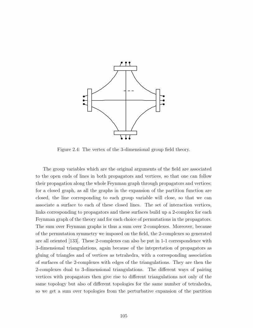
Figure 2.4: The vertex of the 3-dimensional group field theory.

The group variables which are the original arguments of the field are associated

to the open ends of lines in both propagators and vertices, so that one can follow

their propagation along the whole Feynman graph through propagators and vertices;

for a closed graph, as all the graphs in the expansion of the partition function are

closed, the line corresponding to each group variable will close, so that we can

associate a surface to each of these closed lines. The set of interaction vertices,

links corresponding to propagators and these surfaces build up a 2-complex for each

Feynman graph of the theory and for each choice of permutations in the propagators.

The sum over Feynman graphs is thus a sum over 2-complexes. Moreover, because

of the permutation symmetry we imposed on the field, the 2-complexes so generated

are all oriented [133]. These 2-complexes can also be put in 1-1 correspondence with

3-dimensional triangulations, again because of the intepretation of propagators as

gluing of triangles and of vertices as tetrahedra, with a corresponding association

of surfaces of the 2-complexes with edges of the triangulations. They are then the

2-complexes dual to 3-dimensional triangulations. The different ways of pairing

vertices with propagators then give rise to different triangulations not only of the

same topology but also of different topologies for the same number of tetrahedra,

so we get a sum over topologies from the perturbative expansion of the partition

105

function. A crucial question is whether these triangulations are manifolds or not, i.e.

whether it is true that each point of them has a closed neighbourhood homeomorphic

to an n-disc Dn (n = 3 in this case). Precise conditions for the answer to be positive

can be found[137], and translated into conditions on the graphs and it turns out

[137] that in this case all the resulting triangulations are indeed manifolds.

Now let us see what are the amplitudes for each Feynman graph Γ, i.e. for each 2-

complex. If one uses the expressions we gave for propagators and interaction vertices,

it is easy to see that, by integrating the group variables g at the end of each open line

in vertices and propagators (i.e. the original arguments of the field), thus realizing

their gluing, the resulting amplitudes are (we treat the different graphs obtained

from the different terms in the propagators corresponding to different permutations

as different graphs):

Z(Γ) =

(

∏

e∈Γ

∫

dge

)

∏

f

δ(∏

e∈∂fge), (2.57)

i.e. we get a delta function for each face of the dual 2-complex, with argument a

product of SU(2) group elements one for each edge of the 2-complex in the boundary

of the face. This is exaclty the expression for the Ponzano-Regge model as a lattice

gauge theory on the 2-complex!

As in the lattice gauge theory derivation, we could now use this expression to

derive the full spin foam expression for the partition function, expanding each delta

function. However, the spin foam formulation can be derived also directly from the

group field theory, as a “momentum space” expression for the same Feynman graph

amplitudes.

Consider in fact the Fourier decomposition of the field φ:

φ(g1, g2, g3) =∑

j1,j2,j3

∆j1∆j2∆j3 φj1j2j3m1n1m2n2m3n3

Dj1m1n1

(g1)Dj2m2n2

(g2)Dj3m3n3

(g3),(2.58)

with ∆j = 2j + 1, giving then for the gauge invariant field (performing the group

106

integral):

φ(g1, g2, g3) = Pgφ(g1, g2, g3) =

=∑

j1,j2,j3

∆j1∆j2∆j3φj1j2j3m1k1m2k2m3k3

Dj1m1n1

(g1)Dj2m2n2

(g2)Dj3m3n3

(g3)Cj1j2j3n1n2n3

Cj1j2j3k1k2k3

=

=∑

j1,j2,j3

√

∆j1∆j2∆j3 Φj1j2j3m1m2m3

Dj1m1n1

(g1)Dj2m2n2

(g2)Dj3m3n3

(g3)Cj1j2j3n1n2n3

, (2.59)

where the C are the 3j-symbols and we have defined the Fourier components of the

field as Φ = φ123√∆1∆2∆3C

123. Of course the symmetries we imposed on the field

give corresponding symmetries on the Fourier modes.

In terms of this decomposition, the action takes the form:

S[φ] =1

2

∑

j1,j2,j3

| Φj1j2j3m1m2m3

|2 − λ

4!

∑

j1,..,j6

Φj1j2j3m1m2m3

Φj3j5j4m3m5m4

Φj4j2j6m4m2m6

Φj6j5j1m6m5m1

[

j1 j2 j3

j4 j5 j6,

]

(2.60)

from which we easily read out the expression for propagator and potential to be used

in the Feynman expansion. The propagator is just a product of Kronecker deltas

for the representation j’s and the projections m’s, with all the even permutations of

the arguments considered, and the vertex is just given by a 6j-symbol, again with

additional Kronecker delta matching those of the propagators, and responsible for

the correct gluing.

The resulting amplitude for the 2-complex (Feynman graph) Γ is:

Z(Γ) =

∏

f

∑

jf

∏

f

∆jf

∏

v

[

j1 j2 j3

j4 j5 j6

]

v

, (2.61)

exactly the Ponzano-Regge amplitude for the 2-complex Γ!

In the end the partition function for the field theory is therefore:

Z =

∫

dφ e−S[φ] =∑

Γ

λN

sym[Γ]

∏

f

∑

jf

∏

f

∆jf

∏

v

[

j1 j2 j3

j4 j5 j6

]

v

(2.62)

and it has the full structure of a spin foam model, including both a sum over repre-

sentations and a sum over 2-complexes. These 2-complexes as we said correspond to

107

different topologies as well as to different triangulations of the same topology, and

thus the theory defines a full sum-over-histories quantum theory for a 3-dimensional

quantum spacetime. Also, being a spin foam model, it encompasses both the dy-

namical triangulations and quantum Regge calculus approaches to quantum gravity,

incorporating both a sum over triangulations and a sum over metric variables (think

of the asymptotic results).

Of course, the first objection one may have is that we have indeed too much;

in particular, a sum over topologies, although well-defined here as a sum over 2-

complexes and in terms of their fundamental building blocks, can be considered to

be doomed to be badly divergent, being thus physically meaningless and making

mathematically flawed the perturbation expansion. Amazingly, this is not so, and

the sum over 2-complexes can be non-perturbatively defined rigorously by a simple

modification, and this is obtained by adding terms to the sum itself [138]! Indeed,

it can be shown [138] that simply by adding a term like

α [Ph1φ(g1, g2, g3)][Ph2φ(g3, g5, g4)][Ph3φ(g4, g5, g6)][Ph4φ(g6, g2, g1)] (2.63)

as an additional interaction term in the action for the field, the corresponding par-

tition function is Borel summable when given in terms of a perturbative expansion

of Feynman graphs. The modified model amounts just to a simple generalization of

the Ponzano-Regge model, with the same propagators but with additional possible

vertices of a different combinatorial structure (not having anymore the structure of

tetrahedra) with potentialδj3,j62j3+1

.

The new term has the structure of a “pillow”, i.e. of a set of 4 triangles glued

together in such a way that two pairs of them share a single edge each, while two

other pairs share two edges; it can also be thought of as two tetrahedra glued

together along two common triangles, so that the sum over regular triangulations

(made only with tetrahedra) and irregular traingulations (made using also pillows)

can be re-arranged as a sum over regular triangulations only, but with different

amplitudes.

Not too much is understood of this modified model, but the crucial point is only

that also the sum over topologies that one obtains naturally by means of the group

field theory, and that completes the definition of the spin foam model, can be given

a rigorous meaning with a non-perturbative definition.

108

2.9 Quantum gravity observables in 3d: transi-

tion amplitudes

The field theory over a group gives the most complete definition of the spin foam

models and thus permits us to define and compute a natural set of observables,

namely the n-point functions representing transition amplitudes between eigenstates

of geometry, i.e. spin networks (better s-knots), meaning states with fixed number of

quanta of geometry [139, 140]. We start the discussion of these observables, following

[140], from their definition from a canonical loop quantum gravity point of view, and

then turn to their realization in the field theory over a group framework. We will

give a bit more details about these observables when dealing with the 4-dimensional

case.

The kinematical state space of the canonical theory is given by a Hilbert space of

s-knot states, solutions of the gauge and diffeomorphism constraints, | s〉, includingthe vacuum s-knot | 0〉. We can formally define a projection P : Hdiff → Hphys from

this space to the physical state space of the solutions of the Hamiltonian constraint,

| s〉phys = P | s〉, as we have already discussed. The operator P is assumed to be

real, meaning that 〈s1 ∪ s3 | P | s2〉 = 〈s1 | P | s2 ∪ s3〉, and thus giving invariance

under exchange in the order of the arguments. The ∪ stands for the disjoint union

of two s-knots, which is another s-knot. The quantities

W (s, s′) ≡ phys〈s | s′〉phys = 〈s | P | s′〉 (2.64)

are fully gauge invariant (invariant under the action of all the constraints) objects

and represent transition amplitudes between physical states. We have seen how

a spin foam formalism allows a precise definition of these transition amplitudes,

indirectly defining the projector operator P , without an explicit construction of the

operator P itself. We are about to see how this definition can be phrased in terms

of the group field theory formalism.

We can introduce in Hphys the operator

φs | s′〉phys = | s ∪ s′〉phys (2.65)

with the properties of being self-adjoint (because of the reality of P ) and of satisfying

109

[φs, φs′] = 0, so that we can define

W (s) = phys〈0 | φs | 0〉phys (2.66)

and

W (s, s′) = phys〈0 | φsφs′ | 0〉phys = W (s ∪ s′). (2.67)

In this way we have a field-theoretic definition of the W ’s as n-point functions for

the field φ.

Using the field theory described above, its n-point functions are given, as usual,

by:

W (gi11 , ..., gi1n ) =

∫

Dφ φ(gi11 )...φ(ginn ) e−S[φ], (2.68)

where we have used a shortened notation for the three arguments of the fields φ

(each of the indices i runs over the three arguments of the field).

Expanding the fields φ in “momentum space”, we have [140] the following explicit

(up to a rescaling depending on the representations Ji) expression in terms of the

“field components” Φα1α2α3j1j2j3

:

Wα11α

12α

13

j11j12j

13.....

αn1α

n2α

n3

jn1 jn2 j

n3

=

∫

Dφ φα11α

12α

13

j11j12j

13...φ

αn1α

n2α

n3

jn1 jn2 j

n3e−S[φ]. (2.69)

However, the W functions have to be invariant under the gauge group G to which the

g’s belong, and this requires all the indices α to be suitably paired (with the same

representations for the paired indices) and summed over. Each independent choice

of indices and of their pairing defines an independent W function. If we associate a

3-valent vertex to each φαi1α

i2α

i3

ji1ji2j

i3

with jih at the i-th edge, and connect all the vertices

as in the chosen pairing, we see that we obtain a 3-valent spin network, so that

independent n-point functions W are labelled by spin networks with n vertices.

To put it differently, to each spin network s we can associate a gauge invariant

product of field operators φs

φs =∑

α

∏

n

φα11α

12α

13

j11j12j

13. (2.70)

110

This provides us with a functional on the space of spin networks

W (s) =

∫

Dφ φs e−S[φ] (2.71)

that we can use, if positive definite, to reconstruct the full Hilbert space of the

theory, using only the field theory over the group, via the GNS construction. The

transition functions between spin networks can be easily computed using a pertur-

bative expansion in Feynman diagrams. As we have seen above, this turns out to

be given by a sum over spin foams σ interpolating between the n spin networks

representing their boundaries, for example:

W (s, s′) = W (s ∪ s′) =∑

σ/∂σ=s∪s′A(σ). (2.72)

Let us note that the 2-point functions we discussed are naturally associated

to the Hadamard or Schwinger functions of usual quantum field theory, or of the

relativistic particle, since they do not distinguish between different ordering of the

two arguments and are real functions. They represent a-causal amplitudes between

quantum geometry states, or correlations among them, i.e. they provide their inner

product. They are nevertheless fundamental, fully gauge-invariant, non-perturbative

observables of 3d quantum gravity.

For a different way of using the field theoretical techniques in this context, giving

rise to a Fock space of spin networks on which creation and annihilation operators

constructed from the field act, see [139].

111

Chapter 3

The Turaev-Viro invariant: some

properties

In this section we intend to give more details about the Turaev-Viro invariant, the

most extablished and rigorously defined of the spin foam models discussed so far,

and to show some example of explicit calculations that can be performed with it,

making clear how it involves only combinatorial and algebraic manipulations, while

describing quantum gravity (i.e. geometric and topological) transition amplitudes.

3.1 Classical and quantum 3d gravity, Chern-Simons

theory and BF theory

Let us first recall how different theories can be defined to describe 3d geometry

(gravity)[113], and how they are related to each other at the classical and quantum

level.

Consider first the action for Riemannian first order gravity with positive cosmo-

logical constant in 3d:

Sgr = −∫

M

(

e ∧ F (A) − Λ

6e ∧ e ∧ e

)

(3.1)

The variables are a 1-form e with values in the Lie algebra of SU(2) and a

112

connection 1-form A, with curvature F (A) = dAA again with values in the same Lie

algebra. The gauge group is thus SU(2) (the trace on the Lie algebra is understood

in the action above). Let us recall that in turn this action is a particular instance

of a BF theory action, a topological theory that can be defined in any spacetime

dimension. The solutions of the equations of motion are spaces of constant positive

curvature F = Λ e ∧ e. The group of isometries of the covering space (de Sitter

space) is thus SO(4). We can now define a new gauge connection, with values in

the Lie algebra of Spin(4) ≃ SU(2)× SU(2), by:

A = (A+, A−) A± = A ±√Λ e. (3.2)

The above action can now be re-written as:

Sgr = −∫

M

(

e ∧ F (A) − Λ

6e ∧ e ∧ e

)

= SCS[A] = SCS[A+] − SCS[A

−], (3.3)

where

SCS[A] =k

4π

∫

M

(

A ∧ dA +2

3A ∧ A ∧ A

)

(3.4)

is the action for Chern-Simons theory, which is another topological field theory

in 3d, that can be defined for any gauge group G; here, as we said, G = SO(4)

and k = 4π√Λ. We thus see that 3d gravity with cosmological constant is classically

equivalent to two copies of Chern-Simons theory, with connections each being the

complex conjugate of the other, so any field configuration of the gravitational theory

(in particular any solution of the equation of motion) is in 1-1 correspondence with

a field configuration of the Chern-Simons theory. There is a perfect equivalence

between the two theories at the classical level.

Most important from our point of view is that Witten [61] has shown that a

path integral quantization of the Chern-Simons theory can be obtained, thus using

non-perturbative methods, when the theory is, just as 3d gravity is, perturbatively

non-renormalizable. In other words, the quantum Chern-Simons theory can be

113

defined by means of the partition function:

ZCS =

∫

DAei SCS [A] (3.5)

and this partition function defines by quantum field theoretic means a topological

invariant of 3-manifolds, related to the Jones polynomial [62, 141], called the Chern-

Simons invariant.

At the quantum level, however, the correspondence between gravity and Chern-

Simons theory is more subtle, although one would expect from the considerations

just made that the partition function for 3d gravity with cosmological constant and

gauge group SU(2) would be equal to the modulus squared of the Chern-Simons

partition function for the same gauge group, i.e.:

Zgr[M] =

∫

DADe ei Sgr [e,A] =

∫

DA+DA− ei SCS [A+]− i SCS [A

−] = | ZCS[M] |2 (3.6)

thus giving a different but strictly related topological invariant. The difficulties in

making this correspondence precise are of course in making sense of the path integral

expressions.

Luckily it is indeed possible to make sense of the expressions above by adopting

purely combinatorial and algebraic methods in constructing the above-mentioned

invariants. The rigorously defined topological invariant corresponding to the Chern-

Simons classical theory has been obtained by Reshetikhin and Turaev in [63], using

quantum group techniques and represent an alternative realization of the Chern-

Simons invariant, while the Turaev-Viro invariant we are going to discuss in the

following is the counterpart for the gravity invariant. In fact, while there is no

rigorous construction of the path integral expression for Zgr, and the most direct

connection between the Turaev-Viro spin foam model and 3d gravity is the asymp-

totic calculation for the quantum 6j-symbol we already presented, Roberts [124]

has proven that the Turaev-Viro invariant is given exactly by the modulus square of

the Reshetikhin-Turaev invariant, i.e. the Chern-Simons invariant, and thus realises

precisely the correspondence guessed above. This correspondence can be shown to

be valid also by direct calculations in several instances, with a perfect matching of

continuum calculations based on Chern-Simons theory and combinatorial and al-

gebraic calculations within the Turaev-Viro model, as we are going to show in the

following.

114

3.2 The Turaev-Viro invariant for closed mani-

folds

Let us recall the basic elements of the Turaev-Viro invariant, as exposed already

in section 2.5 (for more details see [66, 123]). The topological invariant for the

3-dimensional manifold is defined by the partition function:

ZTV = Z(T ) = w−2a∑

φ

∏

e

w2e

∏

tet

| 6j |tet, (3.7)

where again φ indicate a coloring of the edges e of the triangulation (faces of the

dual 2-complex) by elements of the set I (representations of SU(2)q), and w and the

we’s are as defined in section 2.5. The basic amplitudes are the quantum 6j-symbols

| 6j |=∣

∣

∣

∣

∣

j1 j2 j3

j4 j5 j6

∣

∣

∣

∣

∣

, that we denote for simplicity of notation

∣

∣

∣

∣

∣

1 2 3

4 5 6

∣

∣

∣

∣

∣

here and in

the following.

These are assumed to possess the following symmetries:

∣

∣

∣

∣

∣

1 2 3

4 5 6

∣

∣

∣

∣

∣

=

∣

∣

∣

∣

∣

2 1 3

5 4 6

∣

∣

∣

∣

∣

=

∣

∣

∣

∣

∣

1 3 2

4 6 5

∣

∣

∣

∣

∣

=

∣

∣

∣

∣

∣

1 5 6

4 2 3

∣

∣

∣

∣

∣

=

∣

∣

∣

∣

∣

4 5 3

1 2 6

∣

∣

∣

∣

∣

=

∣

∣

∣

∣

∣

4 2 6

1 5 3

∣

∣

∣

∣

∣

. (3.8)

In adddition, we assume the following conditions to be verified:

1. (orthogonality)

∑

j

w2j w

24

∣

∣

∣

∣

∣

2 1 j

3 5 4

∣

∣

∣

∣

∣

∣

∣

∣

∣

∣

3 1 6

2 5 j

∣

∣

∣

∣

∣

= δ4,6 (3.9)

for admissible six-tuples;

2. (BE)

∑

j

w2j

∣

∣

∣

∣

∣

2 a j

1 c b

∣

∣

∣

∣

∣

∣

∣

∣

∣

∣

3 j e

1 f c

∣

∣

∣

∣

∣

∣

∣

∣

∣

∣

3 2 4

a e j

∣

∣

∣

∣

∣

=

∣

∣

∣

∣

∣

4 a e

1 f b

∣

∣

∣

∣

∣

∣

∣

∣

∣

∣

3 2 4

b f c

∣

∣

∣

∣

∣

(3.10)

for admissible six-tuples (4, a, e, 1, f, b) and (3, 2, 4, b, f, c);

115

j

a

4

e

1

b

f

c2

3

4b

f1

a

e

3

2

c

Figure 3.1: The geometric interpretation of the Biedenharn-Elliott identity, with

three tetrahedra sharing an edge replaced by two tetrahedra.

3.

∀j ∈ I w2 = w−2j

∑

k,l:(j,k,l)adm

w2k w

2l . (3.11)

While the third condition is a purely algebraic one in nature, the other two have a

geometric intepretation as operations on tetrahedra in the triangulation (as shown

in the picture for the Biedenharn-Elliott identity) and axiomatize the orthogonality

and Biedenharn-Elliott identities for quantum 6j-symbols. Also, the symmetries

imposed on the symbol above correspond to the invariance of the amplitude for a

tetrahedron under the action of the permutation group S4 on the its 4 vertices. As

a result, the amplitude does not register the orientation of the tetraedron itself.

The partition function above can be interpreted, in the context of axiomatic

topological quantum field theories, as a vacuum-to-vacuum transition amplitude,

i.e. as the probability amplitude for a 3-dimensional universe with topology given

by the chosen topology for M. In the case of 3-manifolds with boundaries, instead,

the model provides a function of the boundary triangulations that can be intepreted

as a transition amplitude between quantum states (function of the colorings of the

boundary edges) associated to the boundaries. It is important to stress that the

model does not register the orientation of the manifold considered, and therefore

does not register any order in the states which are the arguments of the transition

amplitude [66].

The above mentioned conditions on the quantum 6j-symbols and on the ampli-

tudes w and wj ’s make the partition function independent of the particular trian-

116

gulation chosen to define it, i.e. imply the fact that ZTV (M) is indeed a topological

invariant characterizing M. In fact, any two triangulations of a given polyhedron

(so of a given topology) can be transformed into one another by a finite sequence of

“Alexander moves” and their inverses [143, 66], and these in turn can be factorised

into three “elementary moves”, one replacing a tetrahedron in the triangulation

with three of them, its inverse, and one changing a pair of tetrahedra into a differ-

ent pair. The Alexander moves can also be formulated in the dual picture, i.e. as

moves changing the 2-skeletons (2-complexes) dual to the triangulations into one

another. It can then be shown [66] that the conditions 1-3) listed above, and satis-

fied by the building blocks of our partition function ZTV , imply its invariance under

the Alexander moves. In other words, the function ZTV (M) evaluates to the same

number for fixed M for any triangulation of it we choose. We can also use this

invariance, and the properties 1-3) to our advantage when evaluating the invariant,

since appropriate sequences of application of the conditions lead to important sim-

plification of the expression we have to evaluate. This will become apparent in the

examples to be shown below.

3.3 Evaluation of the Turaev-Viro invariant for

different topologies

Before showing in details how a non-trivial evaluation of the invariant is performed,

we give a few examples of its values in simple but significant cases.

The simplest case to consider is that of the 3-sphere S3, and the invariant does

not involve any 6j-symbol and evaluates to [66]:

ZTV (S3) = w−4

∑

j

w4j . (3.12)

Another simple case is for M = S1 × S2 for which again we do not need any

6j-symbol and we get [66] simply ZTV = 1.

More interesting, although still simple, is the evaluation of the invariant for the

3-ball B3. In this case, one gets as we said a function of the boundary states, i.e. of

the triangulation of the boundary S2 and of its coloring by representations; therefore

117

4

1

1

2

3

Figure 3.2: A triangulation of B3 using two tetrahedra with the base triangles

identified.

the result can be labelled by using the number of vertices, edges and triangles in the

triangulation of S2 one used. Consider the following three possible triangulations of

B3 [144].

One can triangulate B3 by taking the cone with vertex (4) over two triangles

(123) and (123) joined along the edge (23) and with the opposite vertex (1) identified

(see figure 3.2).

In this case the boundary triangulation has 3 vertices, 3 edges and 2 triangles.

The triangulation of B3 is instead given by 4 vertices, 6 edges and 2 tetrahedra.

The amplitude for the transition ∅ → S2 (or equivalently S2 → ∅) is then given by

[144]:

ZTV (B3, (3, 3, 2), j) = w−5w1w2w3

∑

4,5,6

w24 w

25 w

26

∣

∣

∣

∣

∣

1 2 3

6 5 4

∣

∣

∣

∣

∣

2

=

= w−5w1w2w3

∑

5,6

w25 w

26

w23

= w−3w1w2w3, (3.13)

where we have used orthogonality first and property 3) in the last step.

The most common and simple triangulation of B3 is however given by a single

tetrahedron, whose 4 boundary triangles constitute then a triangulation of S2. The

118

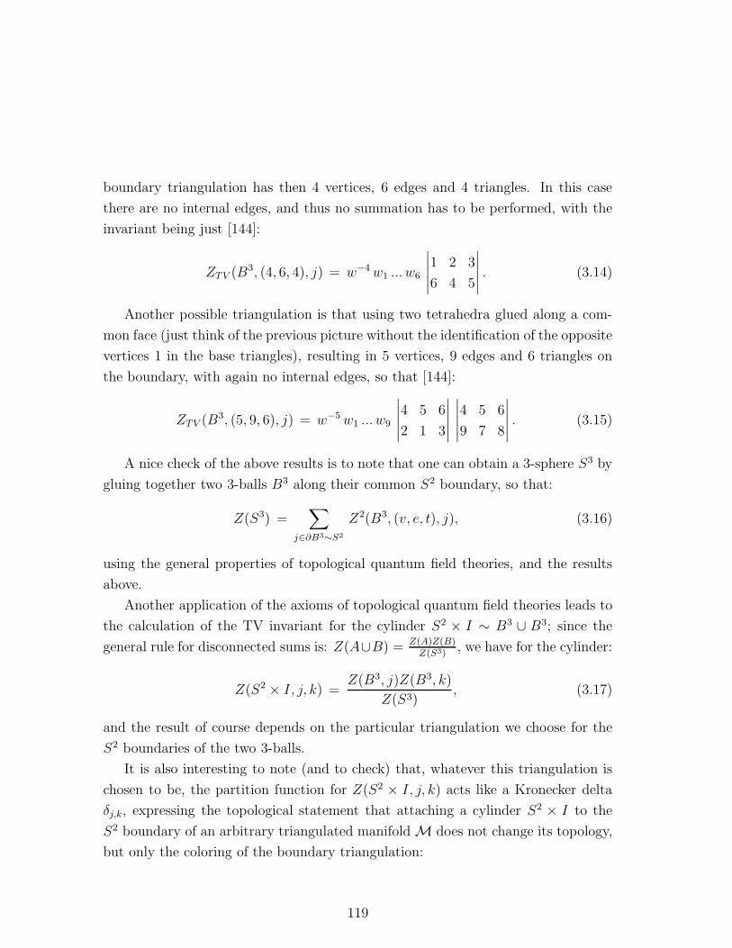
boundary triangulation has then 4 vertices, 6 edges and 4 triangles. In this case

there are no internal edges, and thus no summation has to be performed, with the

invariant being just [144]:

ZTV (B3, (4, 6, 4), j) = w−4w1 ... w6

∣

∣

∣

∣

∣

1 2 3

6 4 5

∣

∣

∣

∣

∣

. (3.14)

Another possible triangulation is that using two tetrahedra glued along a com-

mon face (just think of the previous picture without the identification of the opposite

vertices 1 in the base triangles), resulting in 5 vertices, 9 edges and 6 triangles on

the boundary, with again no internal edges, so that [144]:

ZTV (B3, (5, 9, 6), j) = w−5w1 ... w9

∣

∣

∣

∣

∣

4 5 6

2 1 3

∣

∣

∣

∣

∣

∣

∣

∣

∣

∣

4 5 6

9 7 8

∣

∣

∣

∣

∣

. (3.15)

A nice check of the above results is to note that one can obtain a 3-sphere S3 by

gluing together two 3-balls B3 along their common S2 boundary, so that:

Z(S3) =∑

j∈∂B3∼S2

Z2(B3, (v, e, t), j), (3.16)

using the general properties of topological quantum field theories, and the results

above.

Another application of the axioms of topological quantum field theories leads to

the calculation of the TV invariant for the cylinder S2 × I ∼ B3 ∪ B3; since the

general rule for disconnected sums is: Z(A∪B) = Z(A)Z(B)Z(S3)

, we have for the cylinder:

Z(S2 × I, j, k) =Z(B3, j)Z(B3, k)

Z(S3), (3.17)

and the result of course depends on the particular triangulation we choose for the

S2 boundaries of the two 3-balls.

It is also interesting to note (and to check) that, whatever this triangulation is

chosen to be, the partition function for Z(S2 × I, j, k) acts like a Kronecker delta

δj,k, expressing the topological statement that attaching a cylinder S2 × I to the

S2 boundary of an arbitrary triangulated manifold M does not change its topology,

but only the coloring of the boundary triangulation:

119

∑

j

Z(M, S2, j)Z(S2 × I, j, k) =∑

j

Z(M)Z(B3, j)

Z(S3)

Z(B3, j)Z(B3, k)

Z(S3)(3.18)

=Z(M)Z(B3, k)

Z(S3)

∑

j

Z2(B3, j)

Z(S3)= Z(M, S2, k), (3.19)

where we have used the previous results and the fact that an S2 boundary can be

obtained in a manifold M by simply taking the disjoint union of it with a 3-ball.

This is just an expression of the fact that Z(S2 × I) is a projection operator on the

vector space associated to the surface S2 [60, 69].

We can also compute the partition function for S2 ×S1 starting from this result

by gluing together the two boundaries of a cylinder, recovering the result anticipated

above.

Let us now show a non-trivial evaluation of the Turaev-Viro invariant in full

details. We compute the Turaev-Viro invariant for the 3-torus T 3 ∼ S1×S1×S1. On

the one hand this should make it clear how evaluations of the invariant are performed

in general, on the other hand it provides a check of the correspondence between

the Turaev-Viro and the Chern-Simons invariant, showing how the continuum and

sophisticated calculations of the latter can be reproduced by purely combinatorial

and algebraic methods using the former. The calculation may be tedious but it is

nevertheless absolutely straightforward.

We obtain a triangulation of T 3 by taking a cube, chopping each face into two

triangles, considering one body diagonal, and identifying all the opposite pairs of

edges in each of its faces (see in the figure 3.3).

The resulting triangulation is given by one vertex, seven edges and six tetrahedra.

The partition function is thus given by:

Z(T 3) = w−2∑

1,...,7

w21 ... w

27

∣

∣

∣

∣

∣

3 5 7

4 1 6

∣

∣

∣

∣

∣

∣

∣

∣

∣

∣

3 5 7

1 4 2

∣

∣

∣

∣

∣

∣

∣

∣

∣

∣

4 5 6

1 3 2

∣

∣

∣

∣

∣

∣

∣

∣

∣

∣

4 5 6

3 1 7

∣

∣

∣

∣

∣

∣

∣

∣

∣

∣

2 3 4

7 1 5

∣

∣

∣

∣

∣

∣

∣

∣

∣

∣

2 3 4

6 5 1

∣

∣

∣

∣

∣

.(3.20)

Now we use the inverse of the B-E identity to substitute the 3rd and last tetra-

hedron with three tetrahedra, insering an additional edge labelled by j8:

∣

∣

∣

∣

∣

4 5 6

1 3 2

∣

∣

∣

∣

∣

∣

∣

∣

∣

∣

2 3 4

6 5 1

∣

∣

∣

∣

∣

=∑

8

w28

∣

∣

∣

∣

∣

5 5 8

2 2 1

∣

∣

∣

∣

∣

∣

∣

∣

∣

∣

4 8 4

2 3 2

∣

∣

∣

∣

∣

∣

∣

∣

∣

∣

4 5 6

5 4 8

∣

∣

∣

∣

∣

. (3.21)

120

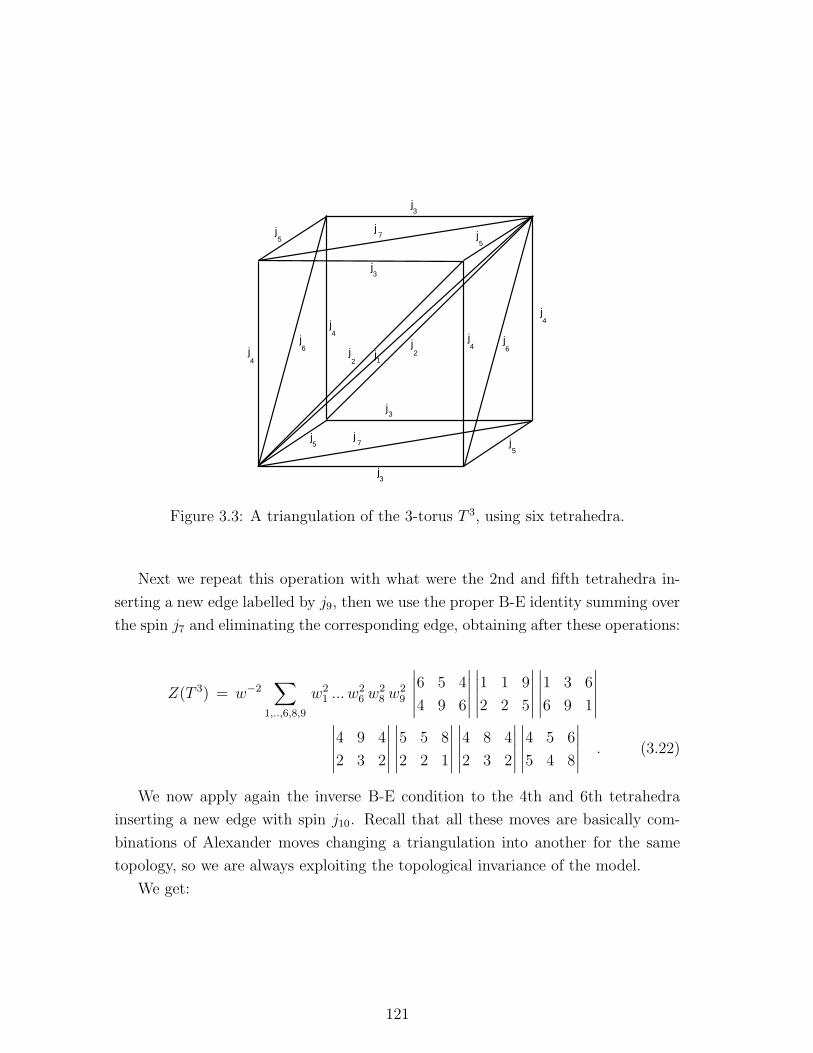
jj

j

j

j

j

j

j

j j1

3

75

4

6

4

5

2

3

j5

j4

j4

j6j

2

j5

j7

j3

j3

Figure 3.3: A triangulation of the 3-torus T 3, using six tetrahedra.

Next we repeat this operation with what were the 2nd and fifth tetrahedra in-

serting a new edge labelled by j9, then we use the proper B-E identity summing over

the spin j7 and eliminating the corresponding edge, obtaining after these operations:

Z(T 3) = w−2∑

1,..,6,8,9

w21 ... w

26 w

28 w

29

∣

∣

∣

∣

∣

6 5 4

4 9 6

∣

∣

∣

∣

∣

∣

∣

∣

∣

∣

1 1 9

2 2 5

∣

∣

∣

∣

∣

∣

∣

∣

∣

∣

1 3 6

6 9 1

∣

∣

∣

∣

∣

∣

∣

∣

∣

∣

4 9 4

2 3 2

∣

∣

∣

∣

∣

∣

∣

∣

∣

∣

5 5 8

2 2 1

∣

∣

∣

∣

∣

∣

∣

∣

∣

∣

4 8 4

2 3 2

∣

∣

∣

∣

∣

∣

∣

∣

∣

∣

4 5 6

5 4 8

∣

∣

∣

∣

∣

. (3.22)

We now apply again the inverse B-E condition to the 4th and 6th tetrahedra

inserting a new edge with spin j10. Recall that all these moves are basically com-

binations of Alexander moves changing a triangulation into another for the same

topology, so we are always exploiting the topological invariance of the model.

We get:

121

Z(T 3) = w−2∑

1,..,6,8,..,10

w21 .. w

26 w

28 w

29 w

210

∣

∣

∣

∣

∣

6 5 4

4 9 6

∣

∣

∣

∣

∣

∣

∣

∣

∣

∣

1 1 9

2 2 5

∣

∣

∣

∣

∣

∣

∣

∣

∣

∣

1 3 6

6 9 1

∣

∣

∣

∣

∣

∣

∣

∣

∣

∣

8 9 10

2 2 2

∣

∣

∣

∣

∣

∣

∣

∣

∣

∣

4 10 4

2 3 2

∣

∣

∣

∣

∣

∣

∣

∣

∣

∣

9 8 10

4 4 4

∣

∣

∣

∣

∣

∣

∣

∣

∣

∣

5 5 8

2 2 1

∣

∣

∣

∣

∣

∣

∣

∣

∣

∣

4 5 6

5 4 8

∣

∣

∣

∣

∣

.(3.23)

And we do the same with the 4th and 6th tetrahedra inserting a new edge with

spin j11, obtaining:

Z(T 3) = w−2∑

1,..,6,8,..,11

w21 .. w

26 w

28 .. w

211

∣

∣

∣

∣

∣

6 5 4

4 9 6

∣

∣

∣

∣

∣

∣

∣

∣

∣

∣

1 1 9

2 2 5

∣

∣

∣

∣

∣

∣

∣

∣

∣

∣

1 3 6

6 9 1

∣

∣

∣

∣

∣

∣

∣

∣

∣

∣

4 2 11

2 4 10

∣

∣

∣

∣

∣

∣

∣

∣

∣

∣

4 4 8

2 2 11

∣

∣

∣

∣

∣

∣

∣

∣

∣

∣

4 10 4

2 9 2

∣

∣

∣

∣

∣

∣

∣

∣

∣

∣

5 5 8

2 2 1

∣

∣

∣

∣

∣

∣

∣

∣

∣

∣

4 5 6

5 4 8

∣

∣

∣

∣

∣

.(3.24)

Up to now the impression may be that we have not simplified the expression for

the invariant at all, and it is indeed the case, but now the partition function has a

form that allows for the simplifications we look for.

We can use orthogonality of the 6j-symbols, by summing over j10, thus elimi-

nating two tetrahedra:

∑

j10

w210w

211

∣

∣

∣

∣

∣

4 10 4

2 9 2

∣

∣

∣

∣

∣

∣

∣

∣

∣

∣

4 2 11

2 4 10

∣

∣

∣

∣

∣

= δ9,11. (3.25)

After this, we eliminate the edge labelled by j8 summing over the corresponding

spin, and we get:

Z(T 3) = w−2∑

1,..,6,9

w21 .. w

26 w

29

∣

∣

∣

∣

∣

6 5 4

4 9 6

∣

∣

∣

∣

∣

∣

∣

∣

∣

∣

1 1 9

2 2 5

∣

∣

∣

∣

∣

∣

∣

∣

∣

∣

1 3 6

6 9 1

∣

∣

∣

∣

∣

∣

∣

∣

∣

∣

4 9 4

2 9 2

∣

∣

∣

∣

∣

∣

∣

∣

∣

∣

6 4 5

2 1 9

∣

∣

∣

∣

∣

∣

∣

∣

∣

∣

5 4 6

9 1 2

∣

∣

∣

∣

∣

.(3.26)

At this stage the partition function has the same complexity as the one we started

with, having again seven edges and six tetrahedra; however, the configuration of

edges is such that two sequences of an inverse B-E move and two orthogonality

moves lead immediately to the final result.

122

This is what we do. We apply the inverse B-E move to the 1st and 3rd tetrahedra,

inserting a new edge with label j7, and then we use orthogonality twice to eliminate

the edges labelled by j3 and j6.

The result is:

Z(T 3) = w−2∑

1,2,4,5,7,9

w21 w

25 w

27 w

29

∣

∣

∣

∣

∣

1 7 4

4 9 1

∣

∣

∣

∣

∣

∣

∣

∣

∣

∣

1 1 9

2 2 5

∣

∣

∣

∣

∣

∣

∣

∣

∣

∣

4 9 4

2 9 2

∣

∣

∣

∣

∣

. (3.27)

The simplification is apparent. We then repeat the same sequence of moves,

by first replacing the 1st and 3rd tetrahedra with three new ones with a new edge

inserted labelled by j3, and then use orthogonality twice to eliminate the spins j7

and j9.

The result do not involve 6j-symbols anymore, and reads:

Z(T 3) = w−2∑

1,2,4,5

w21 w

−22 w2

5. (3.28)

We finally make use of the condition 3):

w−22

∑

1,5

w21 w

25 = w2. (3.29)

The final expression we obtain is:

Z(T 3) =∑

2,4

1. (3.30)

On top of being extremely simple, this result is in agreement with the continuum

calculation perfomed using Chern-Simons theory in [145], confirming the Turaev-

Viro invariant as the square of the Chern-Simons one.

3.4 The Turaev-Viro invariant for lens spaces

In this section we shall compute the Turaev-Viro invariant for more interesting

manifolds than the ones considered so far, showing how it encodes their topological

123

properties. The manifolds we consider are lens spaces, denoted Lp,q, where p and q

are integers.

Lens spaces [144, 146] are 3-manifolds with genus 1 Heegaard splitting, i.e. they

are constructed out of two solid tori H1 = D2×S1 by gluing them along the common

boundary T 2 = S1 × S1 with an appropriate homeomorphism hp,q : T 2 → T 2:

Lp,q = H1 ∪hp,q H1. The homeomorphism is defined as follows: calling m and l the

meridian and longitudinal circles of T 2, hp,q is defined as the identification of the

meridian m of one torus with the curve winding p times long the longitude and q

times along the meridian of the second torus, with p, q ∈ Z:

hp,q : m → p l + q m. (3.31)

In addition to the interest in lens spaces from a purely topological point of view,

that will be our concern in the following, we note also that, being prime manifolds

[147], lens spaces have an interpretation as geons [148], i.e. topologically non-trivial

excitation of the metric.

Let us give a few more details on the topology of lens spaces [149]. Lens spaces

Lp,q have fundamental group Zp (so it depends on p only). Two lens spaces Lp,q

and Lp′,q′ are homeomorphic if and only if | p |=| p′ | and q = ±q′ (mod p) or

qq′ = ±1 (mod p). Because of this, we must consider only the cases when p > 1 and

p > q > 0, with p and q relatively prime. Moreover, two lens spaces are homotopic

if and only if | p |=| p′ | and qq′ is, up to a sign, a quadratic residue (mod p).

Therefore, we can have lens spaces that are homotopic but not homeomorphic,

such as L13,2 and L13,5, or that are not homotopic and not homeomorphic but have

the same fundamental group, such as L13,2 and L13,3.

Because of these subtleties, lens spaces provide a very interesting class of manifold

on which to test topological invariants of 3-manifold. In particular they shed light

on the properties of the Chern-Simons invariant and thus on the Turaev-Viro one.

It was conjectured [149] that, when the Chern-Simons invariant ZCS(M) is non-

vanishing, its absolute value | ZCS(M) |=√

ZTV (M) depends only on the funda-

mental group of the manifold M, π1(M).

To the best of our knowledge, there is not yet any proof or disproof of this

conjecture in the general case, but it can indeed be proven for the particular class

of manifolds given by lens spaces, and for the choice of SU(2) as gauge group in

124

the Chern-Simons invariant [149], which is the case we are most interested in from

a quantum gravity perspective. For the case of G = SU(3) only numerical evidence

for the conjecture can be provided [149]. The reason for testing such a conjecture

using lens spaces is of course the mentioned fact that there are examples of lens

spaces which are not homeomorphic (they are not, topologically speaking, the “same

manifold”), but have nevertheless the same fundamental group. In these cases one

would then expect, if the conjecture is true, that the evaluation of the modulus of

the Chern-Simons invariant, and thus of the Turaev-Viro invariant, would give the

same result.

The proof in the case of SU(2) and for a lens space Lp,q is by direct computation

of the invariant [149, 145]. The modulus square of the Chern-Simons invariant, i.e.

the Turaev-Viro invariant, in this case, for level k ≥ 2 is given by the formulae:

ZTV (L2,1) = | ZCS(L2,1) |2= [1 + (−1)k]sin2( π

2k)

sin2(πk)

(3.32)

for p = 2;

ZTV (Lp,q) =1

2[1 − (−1)p]

sin2[π (kφ(p) − 1)k p

]

sin2(πk)

+1

2[1 + (−1)p] [1 + (−1)

p2 ]sin2[π (kφ(p/2) − 1)

k p]

sin2(πk)

,

with p > 2 and where p and k are coprime integers;

ZTV (Lp,q) =g

4 sin2(π/k)[δg(q − 1) + δg(q + 1)], (3.33)

with p > 2 and where the greatest common divisor of p and k, g, is greater than

one, i.e. g > 1, and p/g is odd;

ZTV (Lp,q) =g

4 sin2(π/k)

δg(r + 1) [1 + (−1)kp

2g2 (−1)r+1g ] + δg(r − 1) [1 + (−1)

kp

2g2 (−1)r−1g ]

,

with p > 2 and for g > 1 and p/g even, where we have indicated by φ(n) the Euler

function and by δp(x) the modulo-p Kronecker delta being 0 for x 6= 0 (mod p) and

1 for x = 0 (mod p).

The crucial point is the dependence of ZTV (Lp,q) on q, and it can be shown that,

when ZCS(Lp,q) 6= 0, we have:

ZTV (Lp,q) =1

sin2(π/k)(3.34)

125

for g = 2 and p/g odd,

ZTV (Lp,q) =g

4 sin2(π/k)(3.35)

for g > 2 and p/g odd,

ZTV (Lp,q) =g

2 sin2(π/k). (3.36)

We see that indeed ZTV (Lp,q) =| ZCS(Lp,q) |2 does not depend on the integer q

and is thus a function of the fundamental group Zp only.

The calculations leading to these results are based on surgery presentation of the

lens spaces, and on the expression of the Chern-Simons invariant as a polynomial

invariant (the Jones polynomial) for oriented framed, coloured links embedded in

the continuum manifold. Beautiful as it may be this approach to the evaluation, it

is nevertheless both conceptually and technically quite complex.

The evaluation of the Turaev-Viro invariant for the same manifolds is consid-

erably simpler and really straightforward and it involves only the three basic com-

binatorial and algebraic conditions we discussed and used for the evaluation of the

invariant for the 3-torus.

To write down the TV partition function we have to choose a triangulation of

the lens spaces. This is done as follows [146, 144]. Consider a p-polygon and a

double cone over it, thus obtaining a double solid pyramid glued along the common

polygonal base and thus forming a 3-ball B3. Now identify each point in the upper

half of ∂B3 with a point in the lower half after a rotation by 2πqp

in the base plane

and a reflection with respect to it. The resulting simplicial manifold is indeed a lens

space Lp,q, for relatively prime integers p and q with q < p.

We now give the evaluation of the Turaev-Viro invariant for all the lens spaces

with p up to 9. The calculations for p up to 8 were reported in [66] and [144]. Those

for p = 9 are new.

126

1

1

11

1

1

1

11

2

3

45 6

7

8

9

10

11

1213

14

1516

89

1011

1213

14

15

16

Figure 3.4: A triangulation of the lens space L9,2, obtained with the procedure

described, starting with a 9-polygon, taking a double cone over it, and identifying

upper and lower half points after a rotation of 4π/9 in the base plane and a final

reflection with respect to it.

127

We have:

ZTV (L2,1 ∼ RP 3) = w−2∑

1

w21

ZTV (L3,1) = w−2∑

1:(1,1,1)adm

w21

ZTV (L4,1) = w−2∑

1,2:(1,1,2)adm

w21 w

22

∣

∣

∣

∣

∣

1 1 2

1 1 2

∣

∣

∣

∣

∣

ZTV (L5,1) = w−2∑

1,2,3

w21 w

22 w

23

∣

∣

∣

∣

∣

1 2 3

1 2 1

∣

∣

∣

∣

∣

∣

∣

∣

∣

∣

1 2 3

1 1 3

∣

∣

∣

∣

∣

ZTV (L5,2) = w−2∑

1,2

w21 w

22

∣

∣

∣

∣

∣

1 1 2

1 2 2

∣

∣

∣

∣

∣

ZTV (L6,1) = w−2∑

1,..,4

w21 ... w

24

∣

∣

∣

∣

∣

1 2 3

1 2 1

∣

∣

∣

∣

∣

∣

∣

∣

∣

∣

1 2 3

1 4 3

∣

∣

∣

∣

∣

∣

∣

∣

∣

∣

1 3 4

1 1 4

∣

∣

∣

∣

∣

ZTV (L7,1) = w−2∑

1,..,5

w21 ... w

25

∣

∣

∣

∣

∣

1 4 5

1 1 5

∣

∣

∣

∣

∣

∣

∣

∣

∣

∣

1 4 5

1 4 3

∣

∣

∣

∣

∣

∣

∣

∣

∣

∣

1 2 3

1 2 1

∣

∣

∣

∣

∣

∣

∣

∣

∣

∣

1 2 3

1 4 3

∣

∣

∣

∣

∣

ZTV (L7,2) = ZTV (L7,3) = w−2∑

1,2,3

w21 w

22 w

23

∣

∣

∣

∣

∣

1 2 3

1 2 1

∣

∣

∣

∣

∣

∣

∣

∣

∣

∣

1 2 3

1 3 3

∣

∣

∣

∣

∣

ZTV (L8,1) = w−2∑

1,..,6

w21 ... w

26

∣

∣

∣

∣

∣

1 2 3

1 2 1

∣

∣

∣

∣

∣

∣

∣

∣

∣

∣

1 3 4

1 3 2

∣

∣

∣

∣

∣

∣

∣

∣

∣

∣

1 4 5

1 4 3

∣

∣

∣

∣

∣

∣

∣

∣

∣

∣

1 4 5

1 6 5

∣

∣

∣

∣

∣

∣

∣

∣

∣

∣

1 5 6

1 1 6

∣

∣

∣

∣

∣

ZTV (L8,3) = w−2∑

1,2,3

w21 w

22 w

23

∣

∣

∣

∣

∣

1 2 3

1 2 1

∣

∣

∣

∣

∣

∣

∣

∣

∣

∣

1 2 3

3 2 3

∣

∣

∣

∣

∣

ZTV (L9,1) = w−2∑

1,..,7

w21 ... w

27

∣

∣

∣

∣

∣

7 1 1

7 1 6

∣

∣

∣

∣

∣

∣

∣

∣

∣

∣

6 5 1

6 7 1

∣

∣

∣

∣

∣

∣

∣

∣

∣

∣

1 3 4

1 5 4

∣

∣

∣

∣

∣

∣

∣

∣

∣

∣

1 2 3

2 4 3

∣

∣

∣

∣

∣

∣

∣

∣

∣

∣

1 2 3

2 2 1

∣

∣

∣

∣

∣

∣

∣

∣

∣

∣

4 5 1

6 5 1

∣

∣

∣

∣

∣

ZTV (L9,2) = ZTV (L9,4) = w−2∑

1,..,4

w21 .. w

24

∣

∣

∣

∣

∣

3 2 4

3 2 1

∣

∣

∣

∣

∣

∣

∣

∣

∣

∣

1 2 3

1 2 1

∣

∣

∣

∣

∣

∣

∣

∣

∣

∣

5 2 2

5 2 3

∣

∣

∣

∣

∣

These results are in agreement with those based on Chern-Simons theory [149,

145], of course, and in particular we see the Guadagnini-Pilo result confirmed ex-

plicitely for p = 7 and q = 2, 3, and p = 9 and q = 2, 4. It may also be possible to

128

simplify further some of the expressions above by using properties of the quantum

6j-symbols other than the orthogonality and the B-E identity that have been used

here.

129

Chapter 4

Spin foam models for

4-dimensional quantum gravity

We turn now to the 4-dimensional case. General Relativity in four spacetime di-

mensions is a highly non-trivial theory, not topological anymore in that it possesses

local (although “not localizable”, because of diffeomorphism invariance) degrees of

freedom and is as a consequence much more difficult to quantize. However, it is close

enough to a topological theory that one can make use of many of the techniques

we used to quantize BF theory, and that one can even fit the yet-to-be-constructed

quantum gravity theory in the general formalism of topological quantum field theo-

ries [69, 29], as we shall see. Most important for our concerns, spin foam models for a

4-dimensional spacetime can be obtained along similar lines as in the 3-dimensional

case, and this is indeed the object of the following chapters.

130

4.1 4-dimensional gravity as a constrained topo-

logical field theory: continuum and discrete

cases

The action for General Relativity in the first order formalism is the so-called Palatini

action:

S(e, ω) =

∫

M

∗ e ∧ e ∧ F (ω) =

∫

M

ǫIJKL eI ∧ eJ ∧ FKL(ω), (4.1)

where the field variables coming into the action are: a 1-form tetrad field eI = eIµdxµ

with internal R3,1 index I (in R4 in the Riemannian case), giving the spacetime

metric as gµν = ηIJeIµ ⊗ eJν , and a 1-form Lorentz connection ωIJ = ωIJ

µ dxµ with

values in the Lie algebra of the Lorentz group so(3, 1) (so(4) in the Riemannian

case) in the adjoint representation, so that we use the fact ∧2(R3,1) ∼ so(3, 1), with

a 2-form curvature F IJ(ω) = DωIJ . The corresponding equations of motion are:

De = 0, expressing the compatibility of the tetrad field and the connection, i.e. the

fact that the connection we have is a metric connection leaving the metric (tetrad)

field covariantly constant, and e∧F (ω) = 0, being the Einstein equations describing

the dynamics of the spacetime geometry. The symmetries of the action are, just as

in the 3-dimensional case, the usual diffeomorphism invariance and the invariance

under the internal gauge group, i.e. the Lorentz group.

The starting point for the spin foam quantization we are going to discuss is the

fact that this action is classically a subsector of a more general classical action for the

gravitational field, namely the so-called Plebanski action [150, 151], which describes

gravity as a constrained topological theory.

The Plebanski action is a a BF-type action, in the sense that it gives gravity as

a constrained BF theory, with quadratic constraints on the B field. More precisely

the action is given by:

S = S(ω,B, φ) =

∫

M

[

BIJ ∧ FIJ(ω) − 1

2φIJKLB

KL ∧ BIJ

]

(4.2)

where ω is a connection 1-form valued in so(3, 1) (so(4)), ω = ωIJa JIJdx

a, JIJ are

the generators of so(3, 1) (so(4)), F = Dω is the corresponding two-form curvature,

131

B is a 2-form also valued in so(4) (so(3, 1)), B = BIJab JIJdx

a ∧ dxb, and φIJKL

is a Lagrange multiplier, with symmetries φIJKL = φ[IJ ][KL] = φ[KL][IJ ], satisfying

φIJKLǫIJKL = 0.

The equations of motion are:

dB + [ω,B] = 0 F IJ(ω) = φIJKLBKL BIJ ∧ BKL = e ǫIJKL (4.3)

where e = 14!ǫIJKLB

IJ ∧ BKL.

When e 6= 0, i.e. for non-degenerate metric configurations, the constraint (4.3) is

equivalent to ǫIJKLBIJab B

KLcd = ǫabcde [152, 153], which implies that ǫIJKLB

IJab B

KLab =

0 i.e. Bab is a simple bivector. This is the form of the constraint that we are going

to use and that leads to the Barrett-Crane spin foam model. In other words, (4.3)

is satisfied if and only if there exists a real tetrad field eI = eIadxa so that one of the

following equations holds:

I BIJ = ± eI ∧ eJ (4.4)

II BIJ = ± 1

2ǫIJ KLe

K ∧ eL. (4.5)

Restricting the field B to be always in the sector II+ (which is always possible

classically), the action becomes:

S =

∫

M

ǫIJKL eI ∧ eJ ∧ FKL (4.6)

which is the action for General Relativity in the first order Palatini formalism.

Also, the other sector, differing by a global change of sign only, is classically

equivalent to this, while the other two, related by Hodge duality to the “geometric”

ones, corresponds to “pathological geometries” with no physical interpretation (see

the cited literature for more details).

The possibility of this restriction at the classical level was shown in [153], where

it is proven that initial data in the gravity sector do not evolve into any of the

others provided that the tetrad field remains non-degenerate. Therefore we see that

this action defines a diffeomorphism and Lorentz invariant theory, a subsector of

which describes classical General Relativity in the 1st order formalism, as we had

anticipated. This is basically all, as long as the classical level is concerned.

132

The two theories, however, are different at the quantum level, since in the quan-

tum theory one cannot avoid interference between different sectors. In fact in a

partition function for the Plebanski action we have to integrate over all the possi-

ble values of the B field, so considering all the 4 sectors. Another way to see it is

the existence in the Plebanski action of a Z2 × Z2 symmetry B → −B, B → ∗Bresponsible for this interference. This is discussed in [152, 154]. This adds to the

usual subtlety in dealing with a 1st order action, where degenerate configurations

of the metric field cannot be easily excluded, instead of a 2nd order action (metric

or ADM formalism) where one integrates over non-degenerate configurations only.

In particular, the Z2 symmetry between the two geometric sectors of the theory

may affect the path integral quantization of the theory, and the very meaning of

the path integral; remember in fact that a Z2 symmetry on the lapse function

N → −N makes the difference between a path integral realization of the projector

onto solutions of the Hamiltonian constraint and a path integral representing the

Feynman propagator between states, or causal transition amplitude, both in the

relativistic particle case and in quantum gravity in metric formalism, as we have

shown above. A simple argument suggests that this may happen also in our spin

foam context; in fact, a 3 + 1 splitting of the Plebanski action (see [155]), after

the imposition of the constraints on the B field (we are then analysing the 3 + 1

splitting of the Palatini action for gravity), shows that a change of sign in the B

field is equivalent to a change of sign in the lapse function, so that both sectors

of solutions are taken into account in a path integral realization of the projector

operator. The B field has in fact the role of metric field in this BF type formulation

of gravity, and a canonical 3+1 splitting basically splits its independent components

into the triple (hab, Na, N) (with all these expressed in terms of the tetrad field) as

in the usual metric formulation. The reason for and effect of this will be explained

below. Of course, more worrying would be the presence, in the quantum theory, of

the two “non geometric” sectors. We will see that luckily these pathological sectors

do not appear in the quantum theory we are going to discuss in the following.

Before turning to the quantum theory based on the Plebanski action, we have

to discuss in detail the description of simplicial geometry based on it, since it is the

real starting point of the spin foam quantization. In fact, a quantization of gravity

along such lines should start by identifying suitable variables corresponding to the

133

B and ω variables of the Plebanski action, and then the correct translation at the

quantum level of the above constraints on the B field, leading to a realization of the

path integral

Z =∑

M

∫

DBDωDφ ei S(B,A,φ) (4.7)

(we have included a sum over spacetime manifolds), possibly in a not only formal

way. However, both in light of the “finitary” philosophy mentioned above and

hoping to make sense of the path integral by a lattice type of regularization, we pass

to a simplicial setting in which the continuum manifold is replaced by a simplicial

complex, and the continuum fields by variables assigned to the various elements of

this complex.

Just in the same way as in the 3-dimensional case, the connection field is naturally

discretized along the links of the dual complex, by integrating the 1-form connection

along them ωIJ =∫

e∗ ωIJ(x), so that we obtain a holonomy ge∗ (with values in

SO(3, 1) or SO(4)) associated to each link; in this way, again, the curvature is

obtained by choosing a closed path of links, in particular for each dual face we have

a product of group elements gf∗ =∏

e∗⊂∂f∗ ge∗ of the group elements ge∗ associated

with the links of the boundary of the dual face f∗, and it is thus associated with the

dual face itself. This is in turn dual to the triangles of the triangulation T , so we

have the simplicial curvature associated to them, as it is common in 4-dimensional

simplicial gravity. The logarithm of gf∗ gives a Lie algebra element Ωt, the proper

discretization of the curvature field of the Plebanski action.

The crucial point is however the discretization of the B field, since this is what

marks the difference between gravity and BF theory. Being a 2-form, the B field is

naturally discretized along the triangles in the triangulation obtaining a Lie algebra

element associated to each triangle, thus to each face of the dual complex, via

BIJ(t) =∫

tBIJ

µν (x)dxµ ∧ dxν .It is crucial to note that in this discretization, the sign

of the bivector reflects the orientation of the triangle to which it is associated.

With this discretization, the constraints on the B field become constraints on

the bivectors BIJ ∈ so(3, 1) ≃ ∧2(R3,1) associated to the various triangles.

The constraint term in the action is discretized analogously, by integrating over

pairs of triangles, to get: φIJKLBIJ(t)BKL(t′).

134

Therefore, the discrete action we get is:

S(B, ω) =∑

t

trBtΩt +∑

t,t′

φIJKLBIJ(t)BKL(t′). (4.8)

Let us now analyse the constraints on the bivectors more closely. Consider

first a tetrahedron T , whose boundary is made of four triangles t, we have: 0 =∫

TdBIJ(x) =

∫

∂TBIJ(x) =

∑

t

∫

tBIJ(x) =

∑

tBIJ(t) = 0. In other words, the

four bivectors associated to the same tetrahedron sum to zero, as a result of the

tetrahedron being enclosed by the corresponding four triangles.

Consider then the constraints expressed as: ǫIJKLBIJab B

KLcd = ǫabcde, where e =

14!ǫIJKLǫ

abcdBIJab B

KLcd 6= 0 is the spacetime volume element after the imposition of the

constraints, so its being non zero implies that the bivector field is non degenerate.

Integrating this expression of the constraints over pairs of surfaces (triangles) we

obtain [152]:

V (t, t′) =

∫

x∈t,y∈t′

e ǫabcd dxa ∧ dxb ∧ xc ∧ dxd = ǫIJKLB

IJ(t)BKL(t′), (4.9)

where V (t, t′) is obviously the 4-volume spanned by the two triangles t and t′.

This formula clearly implies two constraints on the bivectors associated to the

triangles of the simplicial manifold, corresponding to the two cases in which the

4-volume spanned is zero: each bivector associated to a triangle t satisfies

ǫIJKLBIJ(t)BKL(t) = 0, which corresponds geometrically to the requirement of

the bivector being formed as a vector product of two (edge) vectors, i.e. of being

a “simple” bivector; if we decompose the bivector into its selfdual and anti-selfdual

part (this implies in the Lorentzian case a complexification of the bivector itself),

this constraint also imposes the equality of these two parts; also, for two triangles

sharing an edge, thus belonging to the same tetrahedron, the corresponding bivectors

must be such that ǫIJKLBIJ(t)BKL(t′) = 0, which in turn implies, together with

the previous constraint, that ǫIJKLBIJ(t+ t′)BKL(t+ t′) = 0, i.e. that the bivector

BKL(t+t′) = BKL(t)+BKL(t′) obtained as a sum of the two bivectors corresponding

to the two triangles t and t′ sharing an edge is also a simple bivector. The geometric

meaning of this constraint is to impose that the triangles intersect pairwise in lines

in R3,1, i.e. that they pairwise span 3-dimensional subspaces of R3,1 [110, 118, 111]

135

(this is a rather strong condition in 4 dimensions, since the generic case is for two

surfaces to intersect in a point only).

At the continuum level, as we said, the Plebanski constraints on the bivector

field B make it a geometric field, i.e. put it in correspondence with a tetrad field

and thus with a spacetime metric, so allow for a description of spacetime geometry

in terms of this bivector field; at the discrete level, when the variables we have are

bivectors assigned to the triangles, the above constraints on these bivectors allow

for a description of simplicial geometry in terms of them.

However, the same ambiguity that we have seen at the continuum level for the

solutions of the Plebanski constraints exists at this discretized level, since there are

again four sectors of solutions to these constraints corresponding to the bivectors 1)

BIJ , 2) −BIJ , 3) ∗BIJ = ǫIJKLBKL, 4) −∗BIJ . Again, the cases 1) and 2) correspond

to well-defined simplicial geometries, differing only by a change in orientation, while

the cases 3) and 4) are pathological cases with no geometric interpretation. Again,

we do not consider degenerate configurations. It is possible to distinguish between

these four cases by defining the quantitites:

U± = ±B±(t) · B±(t′) × B±(t′′) (4.10)

for any triple of triangles t, t′ and t′′ sharing an edge, i.e. belonging to the same

tetrahedron, where B±(t) is the selfdual (respectively, anti-selfdual) part of the

bivector associated to the triangle t. In terms of them, the four cases are charac-

terized by [118]: 1) U+ > 0, U− < 0, 2) U+ < 0, U− > 0, 3) U+ > 0, U− > 0, 4)

U+ < 0, U− < 0, and in all these cases we have | U+ |=| U− |. Therefore we can

restrict the configurations considered to the geometric ones by imposing a further

constraint of the form: U+ +U− = 0. This constraint would not come directly from

the discretization of the Plebanski action.

Resuming, the geometry of a 4-simplex, and thus the geometry of a full simplicial

complex (where one glues 4-simplices along common tetrahedra imposing that the

bivector data on the common tetrahedra match), is determined by a set of bivectors

associated to the triangles in the complex and satisfying the following requirements:

• the bivectors change sign when the orientation of the triangles is changed

(orientation constraint);

136

• the bivectors are “simple”, i.e. they satisfy B(t) · ∗B(t) = 0 (simplicity con-

straint);

• the bivectors associated to neighbouring triangles sum to simple bivectors, i.e.

B(t) · ∗B(t′) = 0 if t and t′ share an edge (decomposition constraint);

• the four bivectors associated to the faces of a tetrahedron sum to zero (closure

constraint).

• U+ + U− = 0 (chirality constraint).

The reason why we call the third constraint “decomposition constraint” will become

apparent upon quantization, while the relation of the fifth with issues of chirality

will be clarified in the following. These constraints, together with their quantum

counterparts, were given in [110, 111, 118, 13], while their relation with the Plebanski

formulation of gravity was shown in [152, 153]. We stress again that this description

of simplicial geometry in terms of bivectors, with the associated constraints, holds

in both the Lorentzian and Riemannian case, although in the Lorentzian case the

definition and use of selfdual and anti-selfdual components for the bivectors is less

straightforward since it implies a complexification procedure.

Interestingly, this description of gravity as a constrained BF theory, with quadratic

constraints on the B field, can be generalized to any dimension, at least in the Rie-

mannian case [156]. We will indeed see in the following how the quantum version of

this description can be generalized as well.

In this description, all the geometric quantities such as areas, 3-volumes and

4-volumes have to be expressed in terms of the bivectors. Let us see briefly how this

is done. The easiest objects to consider are the areas of the triangles to which the

bivectors are attached, as they are given simply by the square root of the modulus

of the bivectors themselves:

A(t) =√

B(t) · B(t) =√

BIJ(t)BIJ(t′). (4.11)

The 3-volume V of a tetrahedron can also be expressed in terms of the bivectors

associated to its faces, by taking three of them (which one is left out does not change

the result) and writing:

V 2 = U+ + U−. (4.12)

137

This is indeed the most immediate definition of the (square of the) 3-volume [118,

157]. However, this definition does not reflects the orientation (up or down in R3,1

with respect to the direction normal to the hyperplane in which it is embedded)

of the tetrahedron itself, basically as a consequence of the scalar product (which

is a trace in the Lie algebra if we use the isomorphism ∧2R3,1 ∼ so(3, 1)), while

the 3-volume is indeed a chiral object (it is made out of three bivectors) and should

reflect the orientation of its faces, i.e. whether we have B or −B associated to them.

On the other hand, we have seen that the quantitities U± do reflect this distinction.

As a consequence, with this definition, the 3-volume V would be always zero [157],

so a better definition of the 3-volume operator V would be:

V =√

| U± | = 1

2

(

U+ − U−) . (4.13)

The simplicity constraint, as we said, can be interepreted as imposing the equal-

ity “in norm” of the geometries defined by selfdual and anti-selfdual parts of the

bivectors, but the two descriptions are still different when it comes to orientation

properties of the simplicial structures. This problem is not present for the areas

of the triangles, which are defined by two bivectors and give the same result when

computed using selfdual or anti-selfdual structures.

Let us discuss finally the 4-volume operator for a 4-simplex σ [158, 159]. This

can be given in terms of triangle bivectors as:

Vσ =1

30

∑

t,t′

1

4!ǫIJMN sgn(t, t′)BIJ(t)BMN(t′), (4.14)

where the sum is over all pairs of triangles (t, t′) in σ that do not share a common

edge, with a sign factor sgn(t, t′) depending on their combinatorial orientations.

Let (12345) denote the oriented combinatorial four-simplex σ and (PQRST ) be a

permutation π of (12345) so that t = (PQR) and t′ = (PST ) (two triangles t, t′

in σ that do not share a common edge have one and only one vertex in common).

Then the sign factor is defined by sgn(t, t′) = sgn π [158]. The sum over all pairs of

triangles (t, t′) provides us with a particular symmetrization which can be thought

of as an averaging over the angles that would be involved in an exact calculation of

the volume of a four-simplex. An alternative expression for the four-volume from

138

the context of a first order formulation of Regge calculus [160] is given by,

(Vσ)3 =

1

4!ǫabcdNa ∧Nb ∧Nc ∧Nd, . (4.15)

where the indices a, b, c, d run over four out of the five tetrahedra of the four-simplex

σ (the result is independent of the tetrahedron which is left out), and the Na are

vectors normal to the hyperplanes spanned by the tetrahedra, whose lengths are

proportional to the three-volumes of the tetrahedra. These vectors can of course be

expressed in terms of the bivectors as well [160]. This formula would then involve the

dihedral angles of the 4-simplex, i.e. the angles between the normals to the tetrahe-

dra sharing a triangle, but we did not introduce them in the simplicial description

of the manifold yet. However, they will play a crucial role in the following since they

appear naturally as additional variables corresponding to the Lorentz connection in

the spin foam models we will discuss shortly.

We conclude by noting that, since the basic variables of the theory are associated

to triangles, and thus in some sense one is building the simplicial complex from this

level upwards, a definition of the edge lengths in terms of bivectors or triangle areas

is much less natural.

4.2 Quantum 4-dimensional simplicial geometry

We turn now to the quantization of the simplicial geometry described in terms of

bivectors as given in the previous section. The strategy is just as in the 3-dimensional

case, we obtain a definition of a quantum version of the basic geometric variables, i.e.

of “quantum bivectors” and thus of “quantum triangles”, and then use this to define

quantum states associated to 3-dimensional hypersurfaces in spacetime, obtained

by gluing together tetrahedra along common triangles, thus passing through the

definition of “quantum tetrahedra”. Finally we try to define appropriate quantum

amplitudes to be associated to the 4-simplices, and to be used as building blocks

for the partition function and transition amplitudes between quantum states in the

models that we will derive later on.

The first step is to turn the bivectors associated to the triangles into operators.

To this end, we make use of the isomorphism between the space of bivectors ∧2R3,1

139

and the Lie algebra of the Lorentz group so(3, 1) (or, in the Riemannian case, be-

tween ∧2R4 and so(4) identifying the bivectors associated with the triangles with the

generators of the algebra: BIJ(t) → ∗JIJ(t) = ǫIJ KLJKL. After this preliminary

step we are ready to turn these variables into operators by associating to the differ-

ent triangles t an irreducible representation ρt of the group and the corresponding

representation space, so that the the generators of the algebra act on it (as derivative

operators). In other words, we use a quantization map of the kind: BIJ(t) → ρt, so

that for each triangle we have a Hilbert space and operators acting on it. The rep-

resentation we choose to use are the unitary and (in the Lorentzian case) belonging

to the principal series. While at this stage this choice is rather arbitrary, We will

see in the following how this class of representations is the appropriate choice, basi-

cally because it is that entering in the harmonic analysis for functions on the group

[161, 162, 163], which is the basic tool for both the lattice-gauge theory and the

group field theory derivation of the Barrett-Crane model. The groups we use are in

the Lorentzian case SL(2,C) (the double cover of the proper orthocronous Lorentz

group SO(3, 1)) and in the Riemannian Spin(4) (the double cover of SO(4)). In

the Lorentzian case, the irreducible unitary representations in the principal series

are characterized by a pair (n, ρ) of a natural number n and a real number ρ, while

in the Riemannian case the unitary representations may be characterized by two

half-integers (j1, j2), reflecting the splitting Spin(4) ∼ SU(2)× SU(2).

Therefore we can define the Hilbert space of a quantum bivector to be H =

⊕n,ρH(n,ρ) in the Lorentzian case, and H = ⊕j1,j2H(j1,j2) in the Riemannian. How-

ever, this is not yet the Hilbert space of a quantum geometric triangle, simply

because a set of bivectors does not describe a simplicial geometry unless it satisfies

the constraints we have given in the previous section. The task is then to translate

the above geometric constraints in the language of group representation theory into

the quantum domain.

Of the constraints given for the bivectors, only the first two refer to a triangle

alone, and these are then enough to characterize a quantum triangle. The change

in orientation of the triangle, and the consequent change in sign of the associated

bivector are translated naturally into a map from a given representation ρt and rep-

resentation space Hρt to the dual representation ρ∗t and complex conjugate Hilbert

space Hρ∗t . The most important constraint is however the simplicity constraint, that

140

forces the bivectors to be simple, i..e formed as wedge product of two edge vectors.

Recall that classically this was expressed by: B(t) · ∗B(t) = 0. Now we use the

quantization map given above and substitute the bivectors with the (Hodge dual of

the) Lie algebra elements in the given representation ρt for the triangle t, obtaining

the condition:

J(ρt) · ∗J(ρt) = ǫIJKL JIJ(ρt) J

KL(ρt) = C2(ρt) = 0, (4.16)

i.e. it translates into the condition of having vanishing second Casimir of the group

in the given representation.

For Spin(4) the second Casimir in the representation (j1, j2) is given by: C2 =

j1(j1 +1)− j2(j2 + 1), so that the simplicity constraint forces the selfdual and anti-

selfdual parts to be equal, and we are restricted to considering only representations

of the type (j, j).

For SL(2,C) in the representation (n, ρ) we have for the second Casimir: C2 =

2nρ, so that the only representations satisfying the constraint are those of the form:

(n, 0) and (0, ρ).

In both cases, the type of representations singled out by the simplicity constraint

are the so-called “class 1” representations, realized on the space of functions on

suitable homogeneous spaces, obtained as cosets of the group manifolds with respect

to given subgroups, as we are going to see.

Therefore the Hilbert space of a quantum triangle is given by:

Ht = ⊕nH(n,0) ∪ ⊕ρH(0,ρ) Ht = ⊕jH(j,j), (4.17)

in the Lorentzian and Riemannian cases respectively.

Before considering how this Hilbert space is used to construct that of tetrahedra,

let us discuss briefly the geometric interpretation of the parameters labelling the

representations. Recall that the area of a triangle is given in terms of the associated

bivector by: A2 = B(t) ·B(t), using the quantization map above this translates into:

A2 = JIJ(ρt)JIJ(ρt) = C1(ρt), i.e. the area operator is just the first Casimir of the

group and it is diagonal on each representation space associated to the triangle. Its

eigenvalues are, in the Riemannian case, A2 = C1((j1, j2)) = j1(j1 + 1) + j2(j2 +

1), and in the Lorentzian, A2 = C1((n, ρ)) = n2 − ρ2 − 1. Therefore, for simple

141

representations we have A2 = C1((j, j)) = 2j(j + 1) in the Riemannian, and A2 =

C1((0, ρ)) = −ρ2 − 1 or A2 = C1((n, 0)) = n2 − 1 in the Lorentzian case. In each

case we see that the representation label characterizes the quantum area of the

triangle to which that representation is associated, and also that representations

of the form (0, ρ) correspond to spacelike triangles (we have chosen the signature

(+−−−)), while (n, 0) labels timelike triangles. This timelike/spacelike distinction

is also in perfect agreement with the geometric properties of the corresponding

bivectors, in the sense that the way spacelike and timelike bivectors are summed

in R3,1 is mirrored exactly by the decomposition properties of tensor products of

representations (n, 0) and (0, ρ).

States of the quantum theory are assigned to 3-dimensional hypersurfaces em-

bedded in the 4-dimensional spacetime, and are thus formed by tetrahedra glued

along common triangles. We then have to define a state associated to each tetrahe-

dron in the triangulation, and then define a tensor product of these states to obtain

any given state of the theory. In turn, the Hilbert space of quantum states for the

tetrahedron has to be obtained from the Hilbert space of its triangles, since these

are the basic building blocks at our disposal corresponding to the basic variables of

the theory.

Each tetrahedron is formed by gluing 4 triangles along common edges, and this

gluing is naturally represented by the tensor product of the corresponding repre-

sentation spaces; the tensor product of two representations of SL(2,C) or Spin(4)

decomposes into irreducible representations which do not necessarily satisfy the

simplicity constraint. The third of the constraints on bivectors translates at the

quantum level (using the same procedure as for the simplicity constraint) exactly as

the requirement that only simple (class 1) representations appear in this decompo-

sition. Therefore we are considering for each tetrahedron with given representations

assigned to its triangles a tensor in the tensor product: H1 ⊗H2 ⊗H3 ⊗H4 of the

four representation spaces for its faces, with the condition that the tensored spaces

decompose pairwise into vector spaces for simple representations only. We have

still to impose the closure constraint; this is an expression of the invariance under

the gauge group of the tensor we assign to the tetrahedron, thus in order to fulfill

the closure cosntraint we have to associate to the tetrahedron an invariant tensor,

i.e. an intertwiner between the four simple representations associated to its faces

142

Bρ1ρ2ρ3ρ4 : H1 ⊗H2 ⊗H3 ⊗H4 → C.

It turns out that the last constraint, the chirality constraint, that forbids the

presence of pathological configurations which are however solutions of the other

constraints, is automatically implemented at the quantum level, i.e. that the oper-

ator U+ + U− is identically zero on the space of solutions of the other constraints

[118].

Therefore the Hilbert space of a quantum tetrahedron is given by:

Htet = Inv (H1 ⊗H2 ⊗H3 ⊗H4) , (4.18)

with Hi being the Hilbert space for the i-th triangle defined above. Each state in

this Hilbert space is then a group intertwiner called “the Barrett-Crane intertwiner”

[110, 111]. This construction was rigorously perfomed in [118] in the Riemannian

case, using geometric quantization methods, while the uniqueness of the Barrett-

Crane intertwiner as solution of the geometric constraints was shown in [164].

The Barrett-Crane intertwiner can also be given an integral representation, which

is very useful for both the asymptotic analysis and the geometric interpretation of

the spin foam models we are going to discuss in the following. Moreover, it is this

expression that appears at first in all the derivations of the same models.

In the Riemannian case the simplicity of the representation is equivalent to the

requirement that the representation admits an invariant vector under an SU(2)

subgroup of Spin(4) [161], and the formula is the following:

BJ1J2J3J4k1k2k3k4

= wJ1l1wJ2

l2wJ3

l3wJ4

l4

∫

Spin(4)

dg DJ1l1k1

(g)DJ2l2k2

(g)DJ3l3k3

(g)DJ4l4k4

(g) =

=

∫

Spin(4)/SU(2)∼S3

dxDJ10k1

(x)DJ20k2

(x)DJ30k3

(x)DJ40k4

(x), (4.19)

where the DJilk (g) are matrix elements of the representation function for the group

element g in the representation Ji, one for each triangle, and the wJi are the SU(2)

invariant vectors in the same representation, with which we construct the represen-

tation functions to ensure that the resulting object is invariant under this SU(2) sub-

group; as a consequence, the integral runs only over the coset space Spin(4)/SU(2)

and this is in turn isomorphic to the 3-sphere S3, so that the representation functions

143

themselves can then be considered as functions on the 3-sphere; using the additional

isomorphism S3 ∼ SU(2), one can write the Barrett-Crane intertwiner using SU(2)

representation functions, with the j labelling the simple representations of Spin(4)

(j, j) now interpreted as a label of an SU(2) representation [165].

In the Lorentzian case, there are several realizations of the constraints [111, 167,

168], and we discuss here in more detail only that involving only representations of

SL(2,C) labelled by continuous parameters, i.e. that in which all the triangles and

consequently all the tetrahedra are spacelike. In this case, the simplicity constraint is

realized as invariance under an SU(2) subgroup of SL(2,C), so there exists a timelike

invariant vector in the representation [161, 162], and the formula is analogous:

Bρ1ρ2ρ3ρ4j1k1j2k2j3k3j4k4

= wρ1j′1l1wρ2

j′2l2wρ3

j′3l3wρ4

j′4l4

∫

SL(2,C)

dg Dρ1j′1l1j1k1

(g)Dρ2j′2l2j2k2

(g)Dρ3j′3l3j3k3

(g)Dρ4j′4l4j4k4

(g) =

=

∫

SL(2,C)/SU(2)∼H3

dxDρ100j1k1

(x)Dρ200j2k2

(x)Dρ300j3k3

(x)Dρ400j4k4

(x), (4.20)

where again the Dρ(g) are matrix elements of the representation ρ of the group

element g, and again the w’s are invariant vectors under the SU(2) subgroup; here,

the invariance under SU(2) turns the integral over SL(2,C) into an integral over the

homogeneous space H3, i.e. the upper hyperboloid in Minkowski space. Of course,

in the Lorentzian case, where the integration domain is non compact, we are not

at all guaranteed that the integral makes sense at all. We leave aside this problem

for now, but will comment again on this issue when dealing with spin networks and

with the full spin foam model based on it.

In any case, this invariant tensor represents as we said the state of a tetrahe-

dron whose faces are labelled by the given representations; it can be represented

graphically as in figure 4.1. .

The result is that a quantum tetrahedron is characterized uniquely by 4 parame-

ters, i.e. the 4 irreducible simple representations of so(4) assigned to the 4 triangles

in it, which in turn are interpretable as the (oriented) areas of the triangles. Even if

rigorous, this result is geometrically rather puzzling, since the geometry of a tetra-

hedron is classically determined by its 6 edge lengths, so imposing only the values

of the 4 triangle areas should leave 2 degrees of freedom, i.e. a 2-dimensional mod-

uli space of tetrahedra with given triangle areas. For example, this is what would

144

J

J

J

J

1

4

2

3

J J

J J

1

2 3

4

k

k

k

k

k

k k

k1

2

3

4

1

2 3

4

Figure 4.1: A vertex corresponding to a quantum tetrahedron in 4d, with links

labelled by the representations (and state labels) associated to its four boundary

triangles.

happen in 3 dimensions, where we have to specify 6 parameters also at the quantum

level. So why does a tetrahedron have fewer degrees of freedom in 4 dimensions than

in 3 dimensions, at the quantum level, so that its quantum geometry is characterized

by only 4 parameters? The answer was given in [118], to which we refer for more de-

tails. The essential difference between the 3-dimensional and 4-dimensional cases is

represented by the simplicity constraints that have to be imposed on the bivectors in

4 dimensions. At the quantum level these additional constraints reduce significantly

the number of degrees of freedom for the tetrahedron, as can be shown using geo-

metric quantization [118], leaving us at the end with a 1-dimensional state space for

each assignment of simple irreps to the faces of the tetrahedron, i.e. with a unique

quantum state up to normalization, as we have just seen above. Then the question

is: what is the classical geometry corresponding to this state? In addition to the

four triangle areas operators, there are two other operators that can be character-

ized just in terms of the representations assigned to the triangles: one can consider

the parallelograms with vertices at the midpoints of the edges of a tetrahedron and

their areas, and these are given by the representations entering in the decomposi-

tion of the tensor product of representations labelling the neighbouring triangles.

Analyzing the commutation relations of the quantum operators corresponding to

the triangle and parallelogram area operators, it turns out (see [13, 118]) that while

the 4 triangle area operators commute with each other and with the parallelogram

areas operators (among which only two are independent), the last ones have non-

145

vanishing commutators among themselves. This implies that we are free to specify

4 labels for the 4 faces of the tetrahedron, giving 4 triangle areas, and then only

one additional parameter, corresponding to one of the parallelogram areas, so that

only 5 parameters determine the state of the tetrahedron itself, the other one being

completely randomized, because of the uncertainty principle. Consequently, we can

say that a quantum tetrahedron does not have a unique metric geometry, since there

are geometrical quantities whose value cannot be determined even if the system is in

a well-defined quantum state. In the context of the Barrett-Crane spin foam model,

this means that a complete characterization of two glued 4-simplices at the quantum

level does not imply that we can have all the informations about the geometry of the

tetrahedron they share. This is a very interesting example of the kind of quantum

uncertainty relations that we can expect to find in a quantum gravity theory, i.e. in

a theory of quantum geometry.

A generic quantum gravity state is to be associated to a 3-dimensional hyper-

surface in spacetime, and this will be triangulated by several tetrahedra glued along

common triangles; therefore a generic state will live in the tensor product of the

Hilbert spaces of the tetrahedra of the hypersurface, and in terms of the Barrett-

Crane intertwiners it will be given by a product of one intertwiner BJ1J2J3J4k1k2k3k4

for each

tetrahedron with a sum over the parameters (“angular momentum projections”) la-

belling the particular triangle state for the common triangles (the triangles along

which the tetrahedra are glued). The resulting object will be a function of the simple

representations labelling the triangles, intetwined by the Barrett-Crane intertwiner

to ensure gauge invariance, and it will be given by a graph which has representa-

tions of Spin(4) or SL(2,C) labelling its links and the Barrett-crane intertwiner at

its nodes; in other words, it will be given by a (simple) spin network (see figure 4.2).

We stress that this spin network should not be thought of as embedded anywhere

in the spacetime manifold, but it is just given by the combinatorial data necessary

to determine its graph (and corresponding to the combinatorial structure of a tri-

angulated hypersurface), and by the algebraic data that are its labels on links and

nodes. We will say a bit more on these quantum states later on.

We are left with a last ingredient of a quantum geometry still to be determined:

the quantum amplitude for a 4-simplex σ, interpreted as an elementary change in the

quantum geometry and thus encoding the dynamics of the theory, and representing

146

J

J

J

JJ

JJ

J

J

k

kk

k

k

k

1

1

2

2

3

4

5

6

6

7

7

8 8

9

9

.

Figure 4.2: An example of a (simple) spin network in 4d, with three vertices (to

which the Barrett-Crane intertwiners are associated), and both open and closed

links.

the fundamental building block for the partition function and the transition ampli-

tudes of the theory. As in the 3-dimensional case, this amplitude is to be constructed

out of the tensors associated to the tetrahedra in the 4-simplex, so that it imme-

diately fulfills the conditions necessary to describe the geometry of the simplicial

manifold, at both the classical and quantum level, and has to be of course invari-

ant under the gauge group of spacetime SL(2,C) or Spin(4). The natural choice

is to obtain a C-number for each 4-simplex, a function of the 10 representations

labelling its triangles, by fully contracting the tensors associated to its five tetrahe-

dra pairwise summing over the parameters associated to the common triangles and

respecting the symmetries of the 4-simplex, so:

Aσ : ⊗i Inv(

H1i ⊗H2i ⊗H3i ⊗H4i)

→ C. (4.21)

The amplitude for a quantum 4-simplex is thus, in the Riemannian case:

Aσ = BBC = BJ1J2J3J4k1k2k3k4

BJ4J5J6J7k4k5k6k7

BJ7J3J8J9k7k3k8k9

BJ9J6J2J10k9k6k2k10

BJ10J8J5J1k10k8k5k1

, (4.22)

with the analogous formula holding in the Lorentzian case. We thus obtain as am-

plitude what we may call a 10j-symbol. Clearly it may be seen as the evaluation of a

simple spin network with no open links and with the five vertices contracted follow-

ing the contractions of the Barrett-Crane intertwiners. Of course, in the Lorentzian

147

case the formula for the amplitude will involve several integrals (one for each inter-

twiner) over a non-compact domain and some regularization is needed, and we will

discuss this issue after having obtained the full expression for the partition function

of the Barrett-Crane model.

This amplitude is for fixed representations associated to the triangles, i.e. for

fixed triangle areas; the full amplitude involves a sum over these representations with

the above amplitude as a weight for each configuration. In general, the partition

function of the quantum theory describing the quantum geometry of a simplicial

complex made of a certain number of 4-simplices, will be given by a product of

these 4-simplex amplitudes, one for each 4-simplex in the triangulation, and possibly

additional weights for the other elements of it, triangles and tetrahedra, with a sum

over all the representations assigned to triangles; moreover, also the restriction to

a fixed triangulation ∆ of spacetime has to be lifted, since in this non-topological

case it represents a restriction of the dynamical degrees of freedom of the quantum

spacetime, and a suitably defined sum over triangulations has to be implemented.

We can then envisage a model of the form:

Z(M) =∑

∆

Z(M,∆)BC =∑

∆

∑

J

∏

triangles

Atr

∏

tetrahedra

Atet

∏

4−simpl

BBC , (4.23)

or, if one sees all the data as assigned to the 2-complex ∆∗ dual to the triangulation

∆ (with faces f dual to triangles, edges e dual to tetrahedra, and vertices v dual to

4-simplices):

Z(M) =∑

∆∗Z(M,∆∗)BC =

∑

∆∗

∑

J

∏

f

Af

∏

e

Ae

∏

v

BvBC , (4.24)

clearly with the general structure of a spin foam model.

The above analysis does not allow for a complete specification of the various

amplitudes (although one may certainly guess what amplitudes are most naturally

assigned to triangles and tetrahedra), and we will show now how they can be fully

determined by a lattice gauge theory derivation of the type performed in the 3-

dimensional case.

We close this section by noting that there exists [169] also a quantum deformed

version of the Lorentzian Barrett-Crane model based on the q-deformed Lorentz

148

algebra U(sl(2,C)q [170] and realizing the q-deformed Barrett-Crane intertwiner as

an integral on the quantum hyperboloid H3q [171], in turn described as a pile of

fuzzy 2-spheres. This allows the construction of q-deformed simple spin networks,

out of which the amplitudes for the spin foam model are defined, analogously to

the undeformed case. Also, it is important to note that the quantum deformation

implies that the simple representations of the algebra, including those labelled by a

continuous parameter ρ, take values only in a finite interval in the real line; again, as

in the three dimensional case we have discussed, the quantum deformations provides

a natural cut-off on the allowed representations, and thus an elegant regularization of

the spin foam model. We refer to the original paper for more details. This model is

not only extremely interesting from the purely technical point of view, for the non-

triviality of the construction, but also potentially fundamental from the physical

point of view, since it is believed to be a quantization of the Plebanski action in the

presence of a cosmological constant; the situation would then be similar to the 3-

dimensional case, with the Barrett-Crane model being the analogue of the Ponzano-

Regge model and its quantum deformation being the analogue of the Turaev-Viro

one.

4.3 Discretization and quantum constraints in the

generalized BF-type action for gravity

Before going on to give a derivation of the Barrett-Crane spin foam model, we want

to clarify a further point. We have based the identification of the classical and quan-

tum constraints on the bivectors reducing BF theory to gravity, and consequently of

the Hilbert spaces for triangles and tetrahedra, and finally of the amplitudes for the

4-simplices, on the Plebanski formulation of a gravity theory. However, this is not

the most general formulation of classical gravity as a constrained BF theory, and

we want now to show what, if anything, changes when considering a more general

action of the same kind. The results presented in this section were published in

[154]. Recently, a new action for gravity as a constrained BF theory was proposed

[172] and it seemed that a discretization and spin foam quantization of it would lead

to a model necessarily different from the Barrett-Crane one. Also, a natural out-

149

come would be a one-parameter ambiguity in the corresponding spin foam model,

related to the Immirzi parameter of loop quantum gravity [173][174], and this gives

an additional reason to study the spin foam quantization of the generalized action

since it could help understand the link between the current spin foam models and

loop quantum gravity. We show here that a careful discretization of the new form of

the constraints, an analysis of the field content of the theory, at the classical level,

and a spin foam quantization taking all this into account, lead naturally to the

Barrett-Crane model as a quantum theory corresponding to that action. No one-

parameter ambiguity arises in the spin foam model and in the quantum geometry

described by it. This suggests that the Barrett-Crane model is more universal than

at first thought and that its continum limit may be described by several different

Lagrangians. As we have seen, going from the field theory to the Barrett-Crane

model is achieved in 3 main steps. First, it is the discretization of the two-form into

bivectors associated to each face to the triangulation. Then, we translate bivectors

as elements of so(4)∗ or so(3, 1)∗, using the function

θ : Λ2R4 → so(4)∗ or so(3, 1)∗

e ∧ f → θ(e ∧ f) (l) → η(le, f)(4.25)

where η is the Riemannian or Lorentzian metric. Less formally, it is the step we call

correspondence between bivectors B and elements of the Lie algebra J . The last

step is the quantization itself, using techniques from geometric quantization. This

gives representation labels to the faces of the triangulation and gives the Barrett-

Crane model (up to some normalisation factors). In fact, there is an ambiguity at

the level of the correspondence. We can also choose to use the isomorphism θ tr o∗where ∗ is the Hodge operator. This leads to the so-called flipped Poisson bracket,

and it is indeed the right thing to do. In the Riemannian case, this leads us to

only “real” tetrahedra, whose faces are given by the bivectors and not the Hodge

dual of the bivectors. This amounts to selecting the sector II of the theory which

is the sector we want [118]. In the Lorentzian case, such a check on the tetrahedra

has not been done yet, however the use of the flipped correspondence has a nice

consequence: it changes the sign of the area to being given by −C1 instead of C1

so that the discrete series of representations (n, 0) truly correspond to time-like

faces and the continuous series (0, ρ) to space-like faces, as implied by the algebraic

150

properties of these representations [111]. Using this ambiguity, we can generalize

this correspondence. We have a family of such isomorphisms given by θ tr o(α∗+β).It is this generalized correspondence we are going to use to deal with the generalized

BF-type action. And, at the end, we will find again the same Barrett-Crane model

4.3.1 Generalized BF-type action for gravity

In [172] the following BF-type action was proposed for General Relativity:

S =

∫

BIJ ∧ FIJ − 1

2φIJKLB

IJ ∧ BKL + µH (4.26)

where H = a1φIJIJ +a2φIJKLǫ

IJKL, where a1 and a2 are arbitrary constants. B is a

2-form and F is the curvature associated to the connection ω. φ (spacetime scalar)

and µ (spacetime 4-form) are Lagrange multipliers, with φ having the symmetries

φIJKL = −φJIKL = −φIJLK = φKLIJ . φ enforces the constraints on the B field,

while µ enforces the condition H(φ) = 0 on φ. The ∗ operator acts on internal

indices so that ∗BIJ = 1/2 ǫIJKLBKL and ∗2 = ǫ, with ǫ = 1 in the Riemannian case

and ǫ = −1 in the Lorentzian. Before going on, we would like to point out that this

is indeed the most general action that can be built out of BF theory with a quadratic

constraint on the B field. This in turn means that the scalar constraint H = 0 is

the most general one that can be constructed with a φ with the given symmetry

properties. This can be proven very easily. First of all, we note that the two scalars

φIJIJ and φIJKLǫ

IJKL are linearly independent as it is immediate to verify, so that

what we have to prove is just that the space of scalars made out of φ is 2-dimensional.

There is an easy way to see this in the Riemannian case: φ is a tensor in the 4-

dimensional representation of so(4), which, using the splitting so(4) ≃ su(2)⊕su(2),can be thought of as given by a sum of two 2-dimensional representations of su(2),

that in turn can be decomposed into a sum of a 3-dimensional (and symmetric)

one and a 1-dimensional (and antisymmetric) one. Now we have just to compute

the tensor product of 4 such representations, paying attention to keeping only the

terms with the desired symmetry properties, to see that we can have two and only

two resulting singlets. The equations of motion for ω and B are the same as those

151

coming from the Plebanski action, but the constraints on the field B now are:

BIJ ∧ BKL =1

6(BMN ∧BMN)η

[I|K|ηJ ]L +ǫ

12(BMN ∧ ∗BMN)ǫ

IJKL (4.27)

2a2BIJ ∧ BIJ − ǫa1B

IJ ∧ ∗BIJ = 0 (4.28)

The solution of these constraints [175], for non-degenerate B (BIJ ∧ ∗BIJ 6= 0),

is:

BIJ = α ∗ (eI ∧ eJ) + β eI ∧ eJ (4.29)

with:

a2a1

=α2 + ǫβ2

4αβ(4.30)

Inserting this solution into (4.26), we get:

S = α

∫

∗(eI ∧ eJ ) ∧ FIJ + β

∫

eI ∧ eJ ∧ FIJ (4.31)

so that there is a coupling between the geometric sector given by ∗(e ∧ e) (General

Relativity) and the non-geometric one given by e ∧ e. Nevertheless, we note that

the second term vanishes on shell so that the equations of motion ignore the non-

geometric part and are still given by the Einstein equations. In the usually studied

case a1 = 0, [152][156], we are back to the Plebanski action, the sectors of solutions

being given by α = 0 and β = 0 so that we have either the General Relativity sector

or the non-geometric sector e ∧ e. In the particular case a2 = 0, in the Riemannian

case, the only solution to (4.30) is α = β = 0 so that only degenerate tetrads are

going to contribute. On the other hand, in the Lorentzian case we have instead

α = ±β.Looking at 4.30, once we have chosen a pair (α, β), we see that we have four

posible sectors as with the Plebanski action [152]. In the Riemannian case, we can

exchange α and β. Under this transformation, the B field gets changed into its

Hodge dual, so we can trace back this symmetry to the fact that we can use both B

and ∗B as field variables in our original action, without any change in the physical

152

content of the theory. We can also change B → −B without affecting the physics

of our model. This gives us the following four sectors:

(α, β) (−α,−β) (β, α) (−β,−α) (4.32)

In the Lorentzian case, the same ∗-symmetry brings us the following four sectors:

(α, β) (β,−α) (−α,−β) (−β, α) (4.33)

The canonical analysis of the action (4.31) was performed in [176], leading to the

presence of the Immirzi parameter of loop quantum gravity given by γ = α/β and

related to a1 and a2 by:

a2a1

=1

4

(

γ +ǫ

γ

)

(4.34)

We can notice that we have two sectors in our theory with different Immirzi pa-

rameters: γ and ǫ/γ, corresponding to a symmetry exchanging α and ǫβ. The full

symmetry group of the theory is then Diff(M) × SO(4) × Z2 × Z2, with SO(4)

replaced by SO(3, 1) in the Lorentzian case. The Z2×Z2 comes from the existence of

the four sectors of solutions and is responsible for their interferences at the quantum

level.

We want to study the relationship between this new action and the usual Ple-

banski action, and its spin foam quantization, in order to understand if and in which

cases the corresponding spin foam model at the quantum level is still given by the

Barrett-Crane one. To this aim it is important to note that the constraints (4.27)

and 4.28 can be recast in an equivalent form leading to the same set of solutions,

for a2 6= 0, B non-degenerate, and(

a12a2

)2

6= ǫ (this excludes the purely selfdual and

the purely anti-selfdual cases). The situation is analogous to that analyzed in [152]

for the Plebanski action. The new constraint is(

ǫIJMN − a1a2η[I|M |ηJ ]N

)

BMNcd BIJ

ab = e ǫabcd

(

1− ǫ

(

a12a2

)2)

(4.35)

where

e =1

4!ǫIJKLB

IJ ∧ BKL (4.36)

153

This constraint can then be discretised to give the simplicity constraint and the

intersection constraint leading to the Barrett-Crane model, as we will see in section

(4.3.2). But we can already notice that in the case (ab) = (cd), (4.37) gives an

equivalent to (4.28):

2a21

2ǫIJKLB

IJabB

KLab − a1BIJabB

abIJ = 0 (4.37)

In the following, we mainly use this second form of the constraints, discussing the

discretization and possible spin foam quantization of the first one in section (4.3.4).

Looking at the constraints on B it is apparent that they are not anymore just

simplicity constraints as in the Plebanski case, so that a direct discretization of them

for B would not give the Barrett-Crane constraints. We can see this by translating

the constraints into a condition on the Casimirs of so(4) (or so(3, 1)), using the

isomorphism between bivectors and Lie algebra. We can naively replace BIJab with

the canonical generators JIJ of so(4) (or so(3, 1)), giving the correspondence:

BIJab B

abIJ → JIJJIJ = 2C1 (4.38)

1

2ǫIJKLB

IJab B

KLab → 1

2ǫIJKLJ

IJJKL = 2C2 (4.39)

Using this, (4.37) gets transformed into:

2a2C2 − a1C1 = 0 (4.40)

or equivalently:

2αβC1 = (α2 + β2)C2 (4.41)

Then we would conclude as suggested in [172] that we should use non-simple repre-

sentations in our spin foam model. Actually the situation would be even worse than

this, since it happens that in general (for arbitrary values of a1 and a2) no spin foam

model can be constructed using only representations satisfying (4.40) in the Rieman-

nian case. More precisely, using the splitting of the algebra so(4) ≃ su(2)+⊕su(2)−,the two Casimirs are:

154

C1 = j+(j+ + 1) + j−(j− + 1)

C2 = j+(j+ + 1)− j−(j− + 1) (4.42)

Apart from the case a1 = 0 which gives us the Barrett-Crane simplicity constraint

C2 = 0, the equations (4.40) have an infinite number of solutions only when 2a2 =

±a1, in which cases we get representations of the form (j+, 0) (or (0, j−)). This could

be expected since the constraint (4.28) with this particular value of the parameters

implies that the B field is selfdual or anti-selfdual when non-degenerate. In the other

cases, (4.40) can be written as j+(j++1) = λj−(j−+1), with 2a2 = (1+λ)/(1−λ)a1and in general has no solutions. For particular values of λ, it can have one and only

one solution. This would lead us to an ill-defined spin foam model using only one

representation (j+0 , j−0 ). However, using the framework set up in [164], it can be

easily proven that it is not possible to construct an intertwiner for a spin network

built out of a single representation (a single representation is not stable under change

of tree expansion for the vertex) so that no spin foam model can be created.

In the Lorentzian case, the situation is more complex. The representations are

labelled by pairs (j ∈ N/2, ρ ≥ 0) and the two Casimirs are [168][162]:

C1 = j2 − ρ2 − 1

C2 =1

2jρ (4.43)

The equation (4.40) now reads:

ρ2 +a2a1jρ− j2 + 1 = 0 (4.44)

and admits the following solutions if a1 6= 0:

ρ =1

2

−a2a1j ±

√

(

a2a1

)2

j2 + 4(j2 − 1)

(4.45)

So we always have some solutions to the mixed simplicity condition (4.40). However,

instead of having a discrete series of representations (n, 0) and a continuous series

155

(0, ρ), which are said to correspond to space-like and time-like degrees of freedom, as

in the simple case a1 = 0, we end up with a (couple of) discrete series representations

with no direct interpretation. We think it is not possible to construct a consistent

vertex using them (it is also hard to imagine how to construct a field theory over a

group manifold formulation of such a theory whereas, in the case of simple repre-

sentations, the construction was rather straightforward [134, 167, 168] adapting the

Riemannian case to the Lorentzian case). But this should be investigated. As we

will show, on the contrary, a careful analysis of the field content of the theory, and of

the correspondence between Lie algebra elements and bivectors shows that not only

a spin foam quantization is possible, but that the resulting spin foam model should

again be based on the Barrett-Crane quantum constraints on the representations.

4.3.2 Field content and relationship with the Plebanski ac-

tion

We have seen that the B field, even if subject to constraints which are more compli-

cated than the Plebanski constraints, is forced by them to be in 1-1 correspondence

with the 2-form built out of the tetrad field, ∗(e∧ e), which in turn is to be consid-

ered the truly physical field of interest, since it gives the geometry of the manifold

through the Einstein equations. To put it in another way, we can argue that the

physical content of the theory, expressed by the Einstein equations, is independent

of the fields we use to derive it. In a discretized context, in particular, we know that

the geometry of the manifold is captured by bivectors associated to 2-dimensional

simplices, and constrained to be simple. Consequently we would expect that in this

context we should be able to put the B field in 1-1 correspondence with another

2-form field, say E, then discretize to give a bivector for each triangle, in such a way

that the mixed constraints (4.37) would imply the simplicity of this new bivector

and the other Barrett-Crane constraints. If this happens, then it would also mean

that the action is equivalent to the Plebanski action in terms of this new 2-form

field, at least for what concerns the constraints. This is exactly the case, as we are

going to prove.

The correspondence between B and E is actually suggested by the form of the

solution (4.29). We take

156

BIJab = (α I + ǫ β ∗)EIJ

ab (4.46)

This is an invertible transformation, so that it really gives a 1-1 correspondence, if

and only if α2 − ǫβ2 6= 0, which we will assume to be the case in the following.

Formally, we can do such a change of variable directly on the action and express

the action itself in terms of the field E, making apparent that the constraints are

just the Plebanski constraints:

BIJ = αEIJ + ǫβ ∗ EIJ

φIJKL = (α + ǫβ 12ǫIJ

AB)φABCD(α + ǫβ 12ǫKL

CD)(4.47)

After this change, the action (4.26) becomes:

S =1

|α2 − ǫβ2|3∫

(αEIJ + ǫβ ∗ EIJ) ∧ FIJ − 1

2φIJKLE

IJ ∧ EKL + µǫIJKLφIJKL (4.48)

so that we have the Plebanski constraints on the E field and we can derive directly

from this expression the Holst action (4.31). In the Riemannian case, decomposing

into selfdual and anti-selfdual components can be quite useful to understand the

structure of the theory. This is done in the appendix and shows that the previous

change of variable is simply a rescaling of the selfdual and anti-selfdual parts of the

B field. Let us now look at the discretization of the constraints. We will follow the

same procedure as in [152]. Using the 2-form B, a bivector can be associated to any

2-surface S in our manifold by integrating the 2-form over the surface:

BIJ(S) =

∫

S

BIJ =

∫

S

(α I + ǫ β ∗)EIJ = αEIJ(S) + ǫ β ∗ EIJ(S). (4.49)

Note that this automatically implements the first of the Barrett-Crane constraints

for the bivectors E(S) and B(S) (a change of orientation of the surface S will change

the sign of the bivectors).

We now take a triangulation of our manifold, such that B is constant inside

each 4-simplex, i.e. dB = 0, and we associate a bivector to each triangle of the

157

triangulation using the procedure above. This is equivalent to assuming E constant

in the 4-simplex since the map (4.46) is invertible. Then we can use Stokes’ theorem

to prove that the sum of all the bivectors E associated to the 4 faces t of a tetrahedron

T is zero:

0 =

∫

T

dE =

∫

∂T

E =

∫

t1

E +

∫

t2

E +

∫

t3

E +

∫

t4

E = E(t1) + E(t2) + E(t3) + E(t4) (4.50)

meaning that the bivectors E satisfy the fourth Barrett-Crane constraints (closure

constraint). Let us consider the constraints in the form (4.35). Using (4.46), we

obtain a much simpler constraint on the E field:

(

α2 + ǫ β2)

ǫIJKLEIJab E

KLcd = e ǫabcd (4.51)

Now, e = 14!ǫIJKLB

IJ ∧BKL = 14!(α2 + ǫβ2)ǫIJKLE

IJ ∧EKL is a sensible volume

element, since we assumed that the B field is non-degenerate. After imposing the

equations of motion, it appears that it is also the “right” geometric volume element,

i.e. the one constructed out of the tetrad field. More precisely, equation (4.51)

implies the simplicity of the field E. Thus there exist a tetrad field such that

EIJ = ±eI ∧ eJ or EIJ = ± ∗ (eI ∧ eJ) and this tetrad field is the one defining the

metric after imposing the Einstein equations. The scalar e is then proportional to

ǫIJKLeI ∧ eJ ∧ eK ∧ eL = det(e). Consequently, up to a factor, the 4-volume spanned

by two faces t and t′ of a 4-simplex is given by:

V (t, t′) =

∫

x∈t ; y∈t′

e ǫabcd dxa ∧ dxb ∧ dyc ∧ dyd (4.52)

Then, integrating equation (4.51) gives directly:

ǫIJKLEIJ(t)EKL(t′) =

1

(α2 + ǫ β2)V (t, t′) (4.53)

Considering only one triangle t:

ǫIJKLEIJ(t)EKL(t) = 0 (4.54)

158

so that for any of the bivectors E the selfdual part has the same magnitude as the

anti-selfdual part, so that the E(t) are simple bivectors. This corresponds to the

second of the Barrett-Crane constraints (simplicity constraint). For two triangles

sharing an edge, we similarly have:

ǫIJKLEIJ(t)EKL(t′) = 0 (4.55)

This can be rewritten as:

ǫIJKL(EIJ(t) + EIJ(t′))(EKL(t) + EKL(t′))

−ǫIJKLEIJ(t)EKL(t)− ǫIJKLE

IJ(t′)EKL(t′) = 0 (4.56)

and this, together with the simplicity constraint, implies that the sum of the two

bivectors associated to the two triangles is again a simple bivector. This implements

the third of the Barrett-Crane constraints (intersection constraint). Let us note that

in the Riemannian case, we can use the decomposition into selfdual and anti-selfdual

components to write the previous constraints (for t = t′ or t and t′ sharing an edge)

as:

δIJ[

E(+)I(t)E(+)J (t′)−E(−)I(t)E(−)J (t′)]

= 0 (4.57)

thus showing that the simplicity for the bivectors E(t) and E(t) + E(t′) is that

their selfdual part and anti-self part have the same magnitude. We note that in

the Lorentzian case this decomposition implies a complexification of the fields, so

the physical interpretation is somehow more problematic. However it presents no

problems formally , and corresponds to the splitting of the Lie algebra of so(3, 1),

to which the bivectors in Minkowski space are isomorphic, into su(2)C ⊕ su(2)C.

Thus, it is clear that the complicated constraints (4.27) and (4.37) for the field

B are just the Plebanski constraint for the field E, associated to B by means of

the transformation (4.46), and, when discretized, are exactly the Barrett-Crane

constraints. The fields characterizing the 4-geometry of the triangulated manifold

are then the bivectors E(t). This result, by itself, does not imply necessarily that

a spin foam quantization of the generalized BF-type action gives the Barrett-Crane

model, but it means anyway that the geometry is still captured by a field which, when

159

discretized, gives a set of bivectors satisfying the Barrett-Crane constraints. This in

turn suggests strongly that the Barrett-Crane constraints characterize the quantum

geometry also in this case, even if a first look at the constraints seemed to contradict

this, and consequently the simple representations are the right representations of

so(4) and so(3, 1) that have to be used in constructing the spin foam.

4.3.3 Spin foam quantization and constraints on the repre-

sentations

We have already proven that the spin foam quantization cannot be performed using a

naive association between the B field and the canonical generators of the Lie algebra.

On the other hand, we have seen that the B field can be put in correspondence

with a field E such that the constraints on this are the Barrett-Crane constraints.

This suggest that a similar transformation between Lie algebra elements would make

everything work again, giving again the simplicity conditions for the representations,

as in the Barrett-Crane model.

In light of the natural way to associate a bivector to a triangle in a gravitational

context, using the frame field, and also because the 2-forms ∗(eI ∧eJ ) are a basis for

the space of 2-forms, we could argue that it is the bivector coming from ∗(e∧e) thathas to be associated to the canonical generators of the Lie algebra. That this is the

right choice can be proven easily. In fact the isomorphism between bivectors and

Lie algebra elements is realized choosing a basis for the bivectors such that they are

represented by 4 by 4 antisymmetric matrices, and interpreting these matrices as

being the 4-dimensional representation of Lie algebra elements. If this is done for the

basis 2-forms ∗(e ∧ e), the resulting matrices give exactly the canonical generators

of so(4) or so(3, 1), so that ∗(e ∧ e) ↔ J .

Then equation (4.29) suggests us that the field B has to be associated to elements

J of the Lie algebra such that:

B ↔ JIJ = α JIJ + ǫ β ∗ JIJ (4.58)

This is simply a change of basis (but not a Lorentz rotation), since the trans-

formation is invertible, provided that α2 − ǫβ2 6= 0. In some sense, we can say that

160

working with the B in the action is like working with a non-canonical basis in the

Lie algebra, the canonical basis being instead associated to ∗(e ∧ e).Now we consider the constraint (4.37) on the B field, and use the correspondence

above to translate it into a constraint on the representations of the Lie algebra. The

Casimir corresponding to 12ǫIJKLB

IJab B

abKL is

C2 =1

2ǫIJKLJ

IJ JKL = 2αβC1 + (α2 + ǫβ2)C2 (4.59)

where C1 and C2 are the usual Casimirs associated to the canonical generators JIJ

(being C1 = j+(j+ + 1) + j−(j− + 1) and C2 = j+(j+ + 1) − j−(j− + 1) in the

Riemannian case, and C1 = j2 − ρ2 − 1 and C2 =12jρ in the Lorentzian case), while

the Casimir associated to BIJab B

abIJ is:

C1 = JIJ JIJ = (α2 + ǫβ2)C1 + 2ǫαβC2 (4.60)

Substituting these expressions into (4.37), we get:

2αβC1 = (α2 + ǫβ2)C2 ⇒ (α2 − ǫβ2)2C2 = 0 (4.61)

In the assumed case α2 6= ǫβ2, we find the usual Barrett-Crane simplicity con-

dition C2 = 0 with a restriction to the simple representations of so(4) (j+ = j−) or

so(3, 1) (n = 0 or ρ = 0). We see that, at least for what concerns the representa-

tions to be used in the spin foam model, the whole modification of the inital action

is absorbed by a suitable redefinition of the correspondence between the field B and

the generators of the Lie algebra.

Now we want to discuss briefly how general is the association we used between

the B field and Lie algebra elements, i.e. how many other choices would give still

the Barrett-Crane simplicity constraint on the representations starting from the

constraint (4.37) on the B field. Suppose we associate to B a generic element J of

the Lie algebra, related to the canonical basis by a generic invertible transformation

J = ΩJ . Any such transformation can be split into JIJ = ΩIJKLJ

KL = (αI +

ǫβ∗)IJMNUMNKL JKL = (αI + ǫβ∗)IJMNJ

′MN , for α2 6= ǫβ2, so shifting all the ambiguity

into U . Inserting this into the constraints we obtain the condition C ′2 = 0, where

C ′2 = J ′∗J ′. If we now require that this transformation should still give the Barrett-

Crane simplicity constraint C2 = 0, then this amounts to requiring C ′2 = λC2 for

161

a generic λ. But if C2 = 0 and the transformation preserves the second Casimir

modulo rescaling, then it should preserve, modulo rescaling, also the first one. This

means that the transformation U preserves, modulo rescaling, the two bilinear forms

in the Lie algebra which the two Casimirs are constructed with, i.e. the “identity”

and the completely antisymmetric 4-tensor in the 6-dimensional space of generators.

Consider the Riemannian case. The set of transformations preserving the first is

given by O(6)×Z2 ≃ SO(6)× Z2 × Z2, while the set of transformations preserving

the second is given by O(3, 3)× Z2 ≃ SO(3, 3)× Z2 × Z2, so that the U preserving

both are given by the intersection of the two groups, i.e. by the transformations

belonging to a common subgroup of them. Certainly a common subgroup is given

by SO(3)× SO(3)× Z2 × Z2 ≃ SO(4)× Z2 × Z2, and we can conjecture that this

is the largest one, since it covers all the symetries of the original action, so that

any solution of the theory, like (4.29) should be defined up to such transformation,

and we expect this to be true also in the association between fields and Lie algebra

elements. Of course we can in addition rescale the J with an arbitrary real number.

The argument in the Lorentzian case goes similarly.

Coming back to the spin foam model corresponding to the new generalized action,

our results prove that it should still be based on the simple representations of the Lie

algebra, and that no ambiguity in the choice of the labelling of the spin foam faces

results from the more general form of the constraints, since this can be naturally

and unambiguously re-absorbed in the correspondence between the B field and the

Lie algebra elements. This suggests strongly that the resulting spin foam model

corresponding to the classical action here considered is still the Barrett-Crane model,

as for the Plebanski action, but it is not completely straightforward to prove it due

to the more complicated form of the action (4.48). Anyway a motivation for this is

provided by the fact that our analysis shows that the physics is still given by a set of

bivectors E, in 1-1 correspondence with the field B on which the generalized action

is based, and that this bivectors satisfy the Barrett-Crane constraints at the classical

level, with the translation of them at the quantum level being straightforward. The

action is in fact that of BF theory plus constraints, which, as shown in this section,

at the quantum level are just the Barrett-Crane constraints on the representations

used as labelling in the spin foam, so that a spin foam quantization procedure of

the type performed in [177] seems viable.

162

4.3.4 Alternative: the Reisenberger model

We have seen that a natural discretization and spin foam quantization of the con-

straints in this generalized BF-type action leads to the Barrett-Crane model. In this

section we want to discuss and explore a bit the alternatives to our procedure, and

the cases not covered in our previous analysis.

In order to prove the equivalence of the two form of the constraints (4.28) and

(4.37), we assumed that a2 6= 0 and that(

2a2a1

)

6= ǫ, which, in terms of α and

β is requiring that α2 6= ǫβ2 (α 6= ±β in the Riemannian case, and α 6= ±iβin the Lorentzian one). Later, the transformations we used both at the classical

level (B → E) and at the quantum (better, Lie algebra) level (J → J) were well-

defined, i.e. invertible, provided that α2 6= ǫβ2, again. Actually, the only interesting

condition is the last one, since we already mentioned at the beginning (section (4.26))

that the case a2 = 0 leads to considering only degenerate B fields and degenerate

tetrads (in the Riemannian case).

The case(

2a2a1

)

6= ǫ or α2 6= ǫβ2 corresponds, at the canonical level, to the

Barbero’s choice of the connection variable (with Immirzi parameter γ = ±1) in

the Riemannian case, and to Ashtekar variables (γ = ±i) in the Lorentzian case.

It amounts to formulating the theory using a selfdual (or anti-selfdual) 2-form field

B, or equivalently a selfdual (or anti-self dual) connection. In fact, a look at the

constraints (4.28) shows clearly that, in this case, they exactly imply the selfduality

(or anti-selfduality) of the field B. There is no rigorous way to relate the Barrett-

Crane conditions and spin foam model to the classical action when this happens,

at least using our procedure, since the equivalence of (4.28) and (4.37) cannot be

proved and the transformations we used are not invertible. The constraints on the

field B just state that B is the (anti-)selfdual part of a field E (and in this case, the

action (4.26) corresponds to the (anti-)selfdual Plebanski action for E). We note

however that if we use still the constraints in the form (4.37) in the Riemannian case,

in spite of the fact that we are not able to prove their equivalence with the original

ones, and translate them into a constraint on the representations of so(4) using the

naive correspondence B → J , where J is the canonical basis of the algebra, we get:

C1 = ±C2 for 2a2 = ±a1. The first case leads to j− = 0 and the second to j+ = 0,

so we are reduced from so(4) to su(2)L or to su(2)R, with a precise correspondence

163

between the (anti-)selfduality of the variables used and the (anti-)selfduality of the

representations labelling the spin foam. There exist a spin foam model in these cases

as well. It is the Reisenberger model for left-handed (or right-handed) Riemannian

gravity [178][72], whose relationship with the Barett-Crane model is unfortunately

not yet clear. This model [178][158] can be associated to a different discretization of

the generalized action (4.26) using the original form 4.28 of the constraints, as it was

analyzed in [152] for the Plebanski action. This is indeed the only other (known)

alternative to our procedure, at least in the Riemannian case.

As before we define the volume spanned by the two triangles S and S ′:

V (S, S ′) =

∫

x∈S,y∈S′

e ǫabcd dxa ∧ dxb ∧ dyc ∧ dyd (4.62)

To use (4.28), we decompose the 2-form B inside the 4-simplex into a sum of

2-forms associated to the faces (triangles) of the 4-simplex [152][178][179]:

BIJ(x) =∑

S

BIJS (x) (4.63)

where BIJS (x) is such that

∫

BIJS ∧ J = BIJ [S]

∫

S∗

J (4.64)

with J is any 2-form and S∗ the dual face of S (more precisely the wedge dual to

S, i.e the part of the dual face to S lying inside the considered 4-simplex). Then, it

is clear that:∫

S

BIJS′ = δS,S′BIJ [S]

∫

BIJS ∧BKL

S′ = BIJ [S]BKL[S ′]ǫ(S, S ′)

where ǫ(S, S ′) is the sign of the oriented volume V (S, S ′). More precisely ǫ(S, S ′) =

±1 if S, S ′ don’t share any edge, and ǫ(S, S ′) = 0 if they do.

164

Using that, we can translate (4.27) and (4.28) into:

ΩIJKL = ΩIJKL − 1

6η[IKηJ ]LΩAB

AB − 1

24ǫIJKLǫABCDΩ

ABCD = 0 (4.65)

and

4a2ΩABAB = a1ǫABCDΩ

ABCD (4.66)

where

ΩIJKL =∑

S,S′

BIJ [S]BKL[S ′]ǫ(S, S ′) (4.67)

These are the so(4) analogs of the Reisenberger constraints. Let us note that the

constraints involve associations triangles not sharing any edge whereas the Barrett-

Crane procedure was to precisely study triangles sharing an edge i.e being in the

same tetrahedron. This is one of the reasons why it is hard to link these two models.

Then following [72][179], it is possible to calculate the amplitude associated to the

4-simplex and the corresponding spin foam model. For this purpose, it is useful to

project these constraints on the selfdual and anti-selfdual sectors as in [152]:

Ωij++ = Ωij

++ − δij1

3tr(Ω++) = 0 (4.68)

Ωij−− = Ωij

−− − δij1

3tr(Ω−−) = 0 (4.69)

Ωij+− = 0 (4.70)

Ω0 = (α− β)2tr(Ω++) + (α + β)2tr(Ω−−) = 0 (4.71)

The two first constraints are the same as in the Reisenberger model for su(2)

variables. The two last constraints link the two sectors (+ and -) of the theory,

165

mainly stating that there is no correlation between them except for the constraint

Ω = 0. Indeed, only that last constraint is modified by the introduction the Immirzi

parameter. Following the notations of [72], we replace the field BIJ by the generator

JIJ of so(4) (this is a formal quantization of the discretised BF action, see [72] for

more details) and we define the projectors P1,2,3,4 (or some Gaussian-regularised pro-

jectors) on the kernel of the operators corresponding to the four above constraints.

Then, the amplitude for the vertex ν is a function of the holonomies on the 1-dual

skeleton of the three-dimensional frontier ∂ν of the vertex. It is given by projecting

a universal state (or topological state since that without the projectors, the am-

plitude gives the so(4) Ooguri topological model) and then integrating it over the

holonomies around the ten wedges hll=1...10:

a(g∂ν) =

∫

dhl∏

s trwedge

∑

js

trj1⊗···⊗j10

[

P1P2P3P4

⊗

s

(2js + 1)U (js)(g∂s)

]

(4.72)

It seems that a vertex including the Immirzi parameter is perfectly well-defined in

this case. Let us analyse this more closely. As only one constraint involves the

Immirzi parameter, we will first limit ourselves to studying its action. Replacing

the field B by the generators JIJ , we get

Ω0 =∑

S,S′

ǫ(S, S ′)[

(α− β)2J+i[S]J+i[S ′] + (α + β)2 (anti− selfdual)]

=∑

S,S′

ǫ(S, S ′)1

2

[

(α− β)2(

(J+i[S] + J+i[S ′])2 − J+i[S]2 − J+i[S ′]2)

+

+ (α + β)2 (anti− selfdual)]

(4.73)

So Ω0 can be expressed in term of the (su(2)) Casimir of the representations

associated to each wedge S and the Casimir of their tensor products. The difference

from the Barrett-Crane model is that it is the tensor product of the representations

associated to two triangles which do not belong to the same tetrahedron, so there is

little hope of finding directly an equivalent of the simplicity/intersection constraints.

Nevertheless, we can do a naive analysis. Casimirs will always give numbers j(j+1).

But we need to choose a basis of j1⊗· · ·⊗j10. So calculating the action of Ω0 might

166

involve some change of basis and thus some Clebsch-Gordon coefficient. However,

those are still rational. So we conjecture that the amplitude of the vertices will be

zero (no state satisfying Ω0 = 0) except if α = β, α = 0 or β = 0 as in our first

approach to quantizing the B-field constraints in the Barrett-Crane framework. If

this conjecture is verified, we will have two possibilities: either the discretization

procedure is correct and we are restricted to a few consistent cases, or we need to

modify the discretization or quantization procedures.

Resuming, the situation looks as follows. We have the most general BF-type

action for gravity, depending on two arbitrary parameters, both in the Riemannian

and Lorentzian signature. In both signatures, and for all the values of the parameters

except one (corresponding to the Ashtekar-Barbero choice of canonical variables),

the constraints which give gravity from BF theory can be expressed in such a form

that a spin foam quantization of the theory leads to the Barrett-Crane spin foam

model. In the Riemannian case, for all the values of the parameters, a different

discretization, and quantization procedure, leads to the Reisenberger model, but

it also seems that the last spin foam model is non-trivial (i.e. non-zero vertex

amplitude) only for some particular values of the parameters α and β. These two

spin foam models may well turn out to be equivalent, but they are a priori different,

and their relationship is not known at this stage. There is no need to stress that an

analysis of this relationship would be of paramount importance.

4.3.5 The role of the Immirzi parameter in spin foam models

We would like to discuss briefly what our results suggest regarding the role of the

Immirzi parameter in the spin foam models, stressing that this suggestion can at

present neither be well supported nor disproven by precise calculations. As we said

in section (4.3.1), the BF-type action (4.26), after the imposition of the constraints

on the field B, reduces to a generalized Hilbert-Palatini action for gravity, in a form

studied within the canonical approach in [176]. The canonical analysis performed

in that work showed that this action is the Lagrangian counterpart of the Barbero’s

Hamiltonian formulation [180] introducing the Immirzi parameter [173] in the def-

inition of the connection variable and then in the area spectrum. This led to the

suggestion [172] that the spin foam model corresponding to the new action (4.26)

167

would present non-simple representations and an arbitrary (Immirzi) parameter as

well.

On the contrary we have shown that the spin foam model corresponding to the

new action is given again by the Barrett-Crane model, with the representations

labelling the faces of the 2-complex being still the simple representations of so(4) or

so(3, 1). The value of the area of the triangles in this model is naturally given by the

(square root of the) first Casimir of the gauge group in the representation assigned

to the triangle, with no additional (Immirzi) parameter. From this point of view it

can be said that the prediction about the area spectrum of spin foam models and

canonical (loop) quantum gravity do not coincide.

However both the construction of the area operator and its diagonalization imply

working with an Hilbert space of states, and not with their histories as in the spin

foam context, and the canonical structure of the spin foam models, like the Barrett-

Crane one, is not fully understood yet. Consequently, the comparison with the loop

quantum gravity approach and results is not straightforward. In fact, considering

for example the Barrett-Crane model, it assigns an Hilbert space to boundaries of

spacetime, and these correspond, in turn, to boundaries of the spin foam, i.e. spin

networks, so that again a spin network basis spans the Hilbert space of the theory, as

in loop quantum gravity. The crucial difference, however, is that the spin networks

used in the Barrett-Crane model are constructed out of (simple) representations of

so(4) or so(3, 1), i.e. the full local gauge group of the theory, while in loop quantum

gravity (for a nice introduction see [181]) the connection variable used is an su(2)-

valued connection resulting from reducing the gauge group from so(4) or so(3, 1)

to that subgroup, in the process of the canonical 3 + 1 decomposition, so that the

spin network basis uses only su(2) representations. Consequently, a comparison of

the results in spin foam models could possibly be made more easily with a covariant

(with respect to the gauge group used) version of loop quantum gravity, i.e. one in

which the group used is the full so(4) or so(3, 1).

The only results in this sense we are aware of were presented in [183][184]. In

these two papers, a Lorentz covariant version of loop quantum gravity is sketched

at the algebraic level. However, the quantization was not yet achieved and the

Hilbert space of the theory (“spin networks”) not constructed because of problems

arising from the non-commutativity of the connection variable used. Nevertheless,

168

two results were derived from the formalism. The first one is that the path integral

of the theory formulated in the covariant variables is independent of the Immirzi

parameter [183], which becomes an unphysical parameter whose role is to regularize

the theory. The second result was the construction of an area operator acting on

the hypothetic “spin network” states of the theory [184]:

A ≈ l2P√

−C(so(3, 1)) + C(su(2)) (4.74)

where C(so(3, 1)) is a quadratic Casimir of the Lie algebra so(3, 1) (the Casimir C1

to a factor) and C(su(2)) the Casimir of the spatial pull-back so(3). So a “spin

network” state would be labelled by both a representation of so(3, 1) and a repre-

sentation of su(2). As we see, the area, whose spectrum differ from both the the spin

foam and the loop quantum gravity one, is independent of the Immirzi parameter.

However, we do not know yet if such an area spectrum has any physical meaning,

since no Hilbert space has been constructed for the theory. Nevertheless, it suggests

that a “canonical” interpretation of a spin foam might not be as straightforward as

it is believed. Instead of taking as spatial slice an SO(3, 1) spin networks by cutting

a spin foam, we might have to also project the SO(3, 1) structure onto an SU(2)

one; the resulting SU(2) spin network being our space and the background SO(3, 1)

structure describing its space-time embedding.

It is clear that this issue has not found at present any definite solution, and

it remains rather intricate. Thus all we can say is that our results (that do not

regard directly the issue of the area spectrum) and those in [184] suggest that the

appearence of the Immirzi parameter in loop quantum gravity is an indication of

the presence of a quantum anomaly, as discussed in [174], but not of a fundamental

one, i.e. not one originating from the breaking up of a classical symmetry at the

quantum level, and indicating that some new physics takes place. Instead what

seems to happen is that the symmetry is broken by a particular choice of quantization

procedure, and that a fully covariant quantization, like the spin foam quantization

or the manifestly Lorentzian canonical one, does not give rise to any one-parameter

ambiguity in the physical quantities to be measured, i.e. no Immirzi parameter.

Of course, much more work is needed to understand better this issue, in particular

the whole topic of the relationship between the canonical loop quantum gravity

approach and the covariant spin foam one is to be explored in details, and to support

169

or disprove this idea. A crucial step is the appearance of the same kind of simple

spin networks that appear in the Barrett-Crane model in the context of covariant

canonical loop quantum gravity, based on the full Lorentz group, obtained in [185],

about which we will say more later on.

4.4 A lattice gauge theory derivation of the Barrett-

Crane spin foam model

We will now derive the Barrett-Crane spin foam model from a discretization of BF

theory, imposing the constraints that reduce this theory to gravity (the Barrett-

Crane constraints) at the quantum level, i.e. at the level of the representations of

the gauge group used. We perform explicitely the calculations in the Riemannian

case basically only for simplicity of notation, since the same procedure can be used

in the Lorentzian case. We will write down explicitely the Lorentzian version of

the model in a later section. Of course the best thing to do would be to discretize

and quantize directly the Plebanski action, using the discretized expression we have

written down in section 4.1. This is a bit more difficult, due to the non-linearity

of the additional term in the B field (similar problems exist for the discretization

of the BF theory with a cosmological constant, see [120]), but progress along these

lines has been done in [157], leading to the same result as in the simpler procedure,

as we are going to show in the following. The results presented in this section were

published in [177].

4.4.1 Constraining of the BF theory and the state sum for

a single 4-simplex

Consider our 4-dimensional simplicial manifold, and the complex dual to it, having

a vertex for each 4-simplex of the triangulation, an edge (dual link) for each tetra-

hedron connecting the two different 4-simplices that share it, and a (dual) face or

plaquette for each triangle in the triangulation (see figures 4.3 and 4.4).

We introduce a dual link variable ge = eiω(e) for each dual link e, through the

holonomy of the so(4)-connection ω along the link. Consequently the product of

170

f1

f2

f3

f4

e

Figure 4.3: A dual edge e with the four dual faces meeting on it

g1

g2

g3g4

g5

g6

t

f

Figure 4.4: The dual plaquette f for the triangle t

171

dual link variables along the boundary ∂f of a dual plaquette f leads to a curvature

located at the centre of the dual plaquette, i.e. at the center of the triangle t, as

we have already discussed in section 4.1. Dealing also with the B field as we did

there [14, 186, 177, 166], we have [177] the following expression for the discretized

partition function of Spin(4) BF theory:

ZBF (Spin(4)) =

∫

Spin(4)

dg∏

σ

∑

Jσ

∆Jσ χJσ(∏

e

ge) (4.75)

where the first product is over the plaquettes in the dual complex (remember the

1-1 correspondence between triangles and plaquettes), the sum is over (the highest

weight of) the representations of Spin(4), ∆J being their dimension, and χJσ(∏

g)

is the character (in the representation Jσ) of the product of the group elements

assigned to the boundary edges of the dual plaquette σ.

The partition function for the SO(4) BF theory is consequently obtained by

considering only the representation for which the components of the vectors Jσ are

all integers.

We see that the integral over the connection field corresponds to the integral over

group elements assigned to the links of the dual lattice, while the integration over

the B field is replaced by a sum over representations of the group. The meaning

of this can be understood by recalling from the previous sections that, roughly

speaking, the B field turns into a product of tetrad fields after the imposition of

the constraints reducing BF theory to gravity, so giving the geometrical information

about our manifold, and that this information, in spin foam models, has to be

encoded into the algebraic language of representation theory, and be given by the

representations of the gauge group labelling our spin foam.

A generic 4-simplex has 5 tetrahedra and 10 triangles in it (see figure 4.5).

Each dual link goes from a 4-simplex to a neighbouring one through the shared

tetrahedron, so we have 5 dual links coming out from a 4-simplex.

Now we refine the procedure above assigning two dual link variables to each

dual link, dividing it into two segments going from the centre of each 4-simplex

to the centre of the boundary tetrahedron, i.e. we assign one group element g to

each of them (see figure 4.6). Instead of the full plaquette, then, we are considering

“wedges” [178], i.e. the parts of the plaquettes living inside a 4-simplex. In this way

172

1

2

34

54 6 7

73

89

96

2 10

108

51

Figure 4.5: Schematic representation of a 4-simplex; the thick lines represent the 5

tetrahedra and the thin lines the triangles

173

g1

g’1

Figure 4.6: The dual link corresponding to the tetrahedron on which 2 4-simplices

meet

it is possible to deal with manifold with boundaries when the plaquette is truncated

by the boundary, leaving only the wedges inside each 4-simplex.

In other words, a dual plaquette is given by a number, say, m of dual links each

divided into two segments, so there are 2m dual link variables on the boundary

of each plaquette. When a tetrahedron sharing the triangle to which the plaque-

tte corresponds is on the boundary of the manifold, the plaquette results in being

truncated by the boundary, and there will be edges exposed on it (not connecting

4-simplices). To each of these exposed edges we also assign a group variable.

The group variables assigned to the boundary links of each wedge give a curvature

associated to it. Also the B field, or better a representation of the gauge group is

assigned to each wedge. So we have for the partition function of BF theory the same

expression as above, but with a sum over wedges replacing the sum over plaquettes.

We now make use of the character decomposition formula which decomposes the

character of a given representation of a product of group elements into a product of

(Wigner) D-functions in that representation:

χJσ(∏

l∈∂P

ge(l)) =∑

k

∏

i

DJσkiki+1

(gei) , with k1 = k2m+1, (4.76)

where the product on the i index goes around the boundary of the dual plaquette

surrounding the triangle labelled by Jσ, and there is a D-function for each group

element assigned to a dual link and to the edges exposed on the boundary . We

174

choose real representations of Spin(4) (this is always possible). Consider now a

single 4 simplex. Note that in this case all the tetrahedra are on the boundary of

the manifold, which is given by the interior of the 4-simplex. Writing down explicitly

all the products of D-functions and labelling the indices appropriately, we can write

down the partition function for the Spin(4) BF theory on a manifold consisting of a

single 4-simplex in the following way:

ZBF (Spin(4)) =

=∑

Jσ,ke

(

∏

σ

∆Jσ

)

∏

e

∫

Spin(4)

dgeDJe1

ke1me1D

Je2

ke2me2D

Je3

ke3me3D

Je4

ke4me4

(

∏

e

DJil

)

.(4.77)

The situation is now as follows: we have a contribution for each of the 5 edges

of the dual complex, corresponding to the tetrahedra of the triangulation, each of

them made of a product of the 4 D-functions for the 4 representations labelling the

4 faces incident on an edge, corresponding to the 4 triangles of the tetrahedron.

There is an extra product over the faces with a weight given by the dimension of

the representation labelling that face, and the indices of the Wigner D-functions

refer one to the centre of the 4-simplex, one end of the dual edge, and the other to

a tetrahedron on the boundary, the other end of the dual edge. There is also an

additional product of D-functions, one for each group element assigned to an edge

exposed on the boundary, and not integrated over because we are working with fixed

connection on the boundary. The index of the D function on the dual link referring

to the tetrahedron on the boundary is contracted with one index of a D-function for

an element attached to (and only to) a link which is exposed on the boundary. The

other index of each matrix for an exposed link (referring to a triangle) is contracted

with the index coming from the D-function referring to the same triangle (see figure).

It is crucial to note that the group elements attached to the links exposed on the

boundary for each wedge are not integrated over, since we are working with fixed

connection on the boundary, a boundary condition which can be easily shown to

not require any additional boundary term in the classical action (see [120] for the

3-dimensional case).

Now we want to go from BF theory to gravity (Plebanski) theory by imposing

the Barrett-Crane constraints on the BF partition function. These are quantum

175

J

D

D

D

1

1 n 1

J 1

n 1 p 1

J 1

m 1 p1

J 1D1J

k 1 1m

k

Figure 4.7: The assignment of representation functions to the links of a wedge, with

both interior links and links exposed on the boundary

constraints on the representations of SO(4) which are assigned to each triangle of

the triangulation, so they can be imposed at this “quantum” level. The constraints

are essentially two: the simplicity constraint, saying that the representations by

which we label the triangles are to be chosen from the simple representations of

SO(4) (Spin(4)), and the closure constraint, saying that the tensor assigned to each

tetrahedron has to be an invariant tensor of SO(4) (Spin(4)). As we have chosen

real representations, it is easier to impose the first constraint, and the decomposition

constraint will be imposed automatically in the following. We can implement the

simplicity constraint at this level by requiring that all the representation functions

have to be invariant under the subgroup SO(3) of SO(4), so realizing these represen-

tations in the space of harmonic functions over the coset SO(4)/SO(3) ≃ S3, which

is a complete characterization of the simple representations. We then implement the

closure constraint by requiring that the amplitude for a tetrahedron is invariant un-

der a general SO(4) transformation. We note that these constraints have the effect

of breaking the topological invariance of the theory. Moreover, from now on we can

replace the integrals over Spin(4) with integrals over SO(4), and the sum with a sum

over the SO(4) representations only. In the Lorentzian case everything works the

176

same way, with SL(2, C) and SU(2) instead of SO(4) and SO(3) [111, 167], with

the simple representations given in this case by those labelled only by the continuous

parameter ρ.

Note that we are not imposing any projection in the boundary terms, so that

these are the same as those in pure BF theory. However, the projection over simple

representations in the edge amplitude imposes automatically the simplicity also of

the representations entering in the D-functions for the exposed edges.

Consequently we write:

ZBC =∑

Jσ,ke

(

∏

σ

∆Jσ

)

∏

e

∫

SO(4)

dge

∫

SO(3)

dh1

∫

SO(3)

dh2

∫

SO(3)

dh3

∫

SO(3)

dh4

∫

SO(4)

dg′e

DJe1

ke1me1(geh1g

′e)D

Je2

ke2me2(geh2g

′e)D

Je3

ke3me3(geh3g

′e)D

Je4

ke4me4(geh4g

′e)

(

∏

e

D

)

=∑

Jσ,ke

(

∏

σ

dimJσ

)

∏

e

Ae

(

∏

e

D

)

. (4.78)

Let us consider now the amplitude for each edge e of the dual complex (corresponding

to a tetrahedron of the 4-simplex):

Ae =

∫

SO(4)

dge

∫

SO(3)

dh1

∫

SO(3)

dh2

∫

SO(3)

dh3

∫

SO(3)

dh4

∫

SO(4)

dg′e

DJe1

ke1me1(geh1g

′e)D

Je2

ke2me2(geh2g

′e)D

Je3

ke3me3(geh3g

′e)D

Je4

ke4me4(geh4g

′e) (4.79)

for a particular tetrahedron (edge) made out of the triangles 1,2,3,4. Performing

explicitely all the integrals, the amplitude for a single tetrahedron on the boundary

turns out to be:

Ae =∑

simple I,L

1√

∆J1∆J2∆J3∆J4

CJ1J2J3J4Ik1k2k3k4

CJ1J2J3J4Lm1m2m3m4

=1

√

∆J1∆J2∆J3∆J4

BJ1J2J3J4k1k2k3k4

BJ1J2J3J4m1m2m3m4

, (4.80)

177

where the B’s are the (un-normalized) Barrett-Crane intertwiners, ∆J is the dimen-

sion of the representation J of SO(4), and all the representations for faces and edges

in the sum are now constrained to be simple. Considering the usual decomposition

Spin(4) ≃ SU(2)×SU(2) a representation J of SO(4) corresponds, as we said, to a

pair of SU(2) representations (j, k), so that its dimension is (2j + 1)(2k + 1). This

means that a simple representation J of SO(4) would have dimension (2j + 1)2,

where j is the corresponding SU(2) representation. If we had performed only the

integrals over SO(3) we would have obtained the invariant vectors wJ ’s contracting

one index in each D function inside the integrals over the group, and we would

have had exactly the integral expression we have given above for the Barrett-Crane

intertwiners.

Explicitly, the (un-normalized) Barrett-Crane intertwiners are given by [110, 133,

134] (this definition differs by a factor 1√∆1∆2∆3∆4

from the definition as an integral

we have given in the first place, but this is not at all crucial here):

BJ1J2J3J4k1k2k3k4

=∑

simple I

CJ1J2J3J4Ik1k2k3k4

=∑

simple I

√

∆ICJ1J2Ik1k2k

CJ3J4Ik3k4k

(4.81)

where I labels the representation of SO(4) that can be thought as assigned to the

tetrahedron whose triangles are instead labelled by the representations J1, ..., J4,

CJ1J2J3J4Ik1k2k3k4

is an ordinary SO(4) intertwiner between four representations, and finally

CJ1J2Ik1k2k

are Wigner 3j-symbols.

Note that the simplicity of the representations labelling the tetrahedra, i.e. that

appearing in the decomposition of the intertwiner into trivalent ones (the third of

the Barrett-Crane constraints) comes automatically, without the need to impose it

explicitly. We note also that because of the restriction to the simple representations

of the group, the result we end up with is independent of having started from the

Spin(4) or the SO(4) BF partition function.

We see that each tetrahedron on the boundary of the 4-simplex contributes with

two Barrett-Crane intertwiners, one with indices referring to the centre of the 4-

simplex and the other indices referring to the centre of the tetrahedron itself (see

figure 4.8).

The partition function for this theory (taking into account all the different tetra-

178

j1

j2

j2

j1 j4j3

j3 j4

j1

j6

j5

j4

j7

j6

j5

j7

j4

j7

j9j9

j10

j10

j7

j9j9

j10

j10

j1

j3

j3

j8

j8

j6

j2

j6

j2

j8

j5

j8

j5

Figure 4.8: Diagram of a 4-simplex, indicating the two Barrett-Crane intertwiners

assigned to each tetrahedron

hedra) is then given by:

ZBC =∑

J,k,n,l,i,m∆J1...∆J10

1

(∆J1 ...∆J10)

BJ1J2J3J4k1k2k3k4

BJ4J5J6J7l4l5l6l7

BJ7J3J8J9n7n3n8n9

BJ9J6J2J10h9h6h2h10

BJ10J8J5J1i10i8i5i1

BJ1J2J3J4m1m2m3m4

BJ4J5J6J7m4m5m6m7

BJ7J3J8J9m7m3m8m9

BJ9J6J2J10m9m6m2m10

BJ10J8J5J1m10m8m5m1

(

∏

e

D

)

. (4.82)

Now the product of the five Barrett-Crane intertwiners with indices m gives just

the Barrett-Crane amplitude for the 4-simplex to which the indices refer, given by

a 15j-symbol constructed out of the 10 labels of the triangles and the 5 labels of the

tetrahedra (see figure 4.9), so that we can write down explicitly the state sum for a

manifold consisting of a single 4-simplex as:

ZBC =∑

jf,ke′

∏

f

∆jf

∏

e′

Bje′1je′2je′3je′4ke′1ke′2ke′3ke′4

√

∆je′1∆je′2

∆je′3∆je′4

∏

v

BBC

(

∏

e

D

)

, (4.83)

179

j1

j2 j3

j4

j5

j6

j7

j3

j8

j9

j6

j2

j10

j8

j5

j1 j2 j3 j4

j4

j5

j6

j7

j7

j3

j8

j9j9

j6

j2

j10

j10

j8

j5

j1

Figure 4.9: Schematic representation of the Barrett-Crane amplitude for a 4-simplex

where it is understood that there is only one vertex, BBC is the Barrett-Crane

amplitude for a 4-simplex, and the notation e′i means that we are referring to the

face i (in some given ordering) of the tetrahedron e′, which is on the boundary of

the 4-simplex, or equivalently to the i-th 2-simplex of the four which are incident to

the dual edge (1-simplex) e′ of the spin foam (dual 2-complex), which is open, i.e.

not ending on any other 4-simplex. Also the D-functions for the exposed edges are

constrained to be in the simple representation. The boundary terms are given by one

Barrett-Crane intertwiner for each tetrahedron on the boundary, and one D-function

for each group element on each of the exposed edges, contracted with the intertwiner

to form a group invariant, plus a “regularizing” factor in the denominator.

4.4.2 Gluing 4-simplices and the state sum for a general

manifold with boundary

Now consider the problem of gluing two 4-simplices together along a common tetra-

hedron, say, 1234. Having the state sum for a single 4-simplex, we consider two

adjacent 4-simplices separately, so considering the common tetrahedron in the in-

180

terior twice (as being in the boundary of two different 4-simplices), and glue them

together along it.

The gluing is done simply by multiplying the two single partition functions, and

imposing that the values of the representations and of the projections (the ke′i’s) of

the common tetrahedron are of course the same in the two partition functions (this

comes from the integration over the group elements assigned to the exposed edges

that are being glued and become part of the interior, and thus have to be integrated

out). More precisely, the gluing of 4-simplices is now simply done by multiplying

the partition functions for the individual 4-simplices, and integrating over the group

variables that are not anymore on the boundary of the manifold, and required to be

equal in the two 4-simplices, again because we are working with fixed connection on

the boundary, so that the boundary data of the two 4-simplices being glued have

to agree. These group variables appear only in two exposed edges each, and the

orthogonality between D-functions forces the representations corresponding to the

two wedges to be equal:

∫

SO(4)

dgDJkl(g)D

J ′

mn(g) =1

∆J

δkmδlnδJJ ′; (4.84)

moreover, the factors 1∆J

compensate for having two wedges corresponding to the

same triangle, so that to each plaquette of the dual complex, or triangle of the

triangulation, corresponds still only a factor ∆J in the partition function. Finally,

the equality of the matrix indices in the previous relation forces the Barrett-Crane

intertwiners corresponding to the same shared tetrahedron to be fully contracted.

Everything in the state sum is unaffected by the gluing, except for the common

tetrahedron, which now is in the interior of the manifold. In this naive sense we

could say that this way of gluing is local, because it depends only on the parameters

of the common tetrahedron, i.e. it should be determined only by the two boundary

terms which are associated with it when it is considered as part of the two different

4-simplices that are being glued. What exactly happens for the amplitude of this

181

interior tetrahedron is:

∑

m

BJ1J2J3J4m1m2m3m4

√

∆J1∆J2∆J3∆J4

BJ1J2J3J4m1m2m3m4

√

∆J1∆J2∆J3∆J4

=∑

m,I,L

CJ1J2J3J4Im1m2m3m4

CJ1J2J3J4Lm1m2m3m4

(∆J1∆J2∆J3∆J4)2

=∑

I,L

√∆I∆LC

J1J2Im1m2m

CJ1J2Im3m4m

CJ1J2Lm1m2n

CJ3J4Lm3m4n

(∆J1∆J2∆J3∆J4)

=∑

I,L

∆IδILδmn

(∆J1∆J2∆J3∆J4)=∑

I

∆I

(∆J1∆J2∆J3∆J4)=

∆1234

∆J1∆J2∆J3∆J4

(4.85)

where we have used the orthogonality between the intertwiners, and I labels the in-

terior edge (tetrahedron), while the quantity ∆1234 represent the number of possible

intertwiners between the representations J1 − J4.

We see that the result of the gluing is the insertion of an amplitude for the

tetrahedra (dual edges) in the interior of the triangulated manifold, and of course

the disappearance of the boundary terms B since the tetrahedron is not anymore

part of the boundary of the new manifold (see figure 4.10). In other words, the

gluing is not trivial, in the sense that the end result is not just the product of pre-

existing factors, but includes something resulting from the gluing itself (the factor

∆1234).

We can now write down explicitly the state sum for a manifold with boundary

which is then constructed out of an arbitrary number of 4-simplices, and has some

tetrahedra on the boundary and some in the interior, with fixed connection on the

boundary:

ZBC =∑

jf ,ke′

∏

f

∆jf

∏

e′

Bje′1je′2je′3je′4ke′1ke′2ke′3ke′4

√

∆je′1∆je′2

∆je′3∆je′4

∏

e

∆1234

(∆je1∆je2∆je3∆je4)

∏

v

BBC

(

∏

e

D

)

, (4.86)

where the e′ and the e are the sets of boundary and interior edges of the spin

foam, respectively, while the e are the remaining exposed edges, where the bound-

ary connection data are located. The partition function is then a function of the

connection, i.e. of the group elements on the exposed edges.

It is important to note that the number of parameters which determine the gluing

and that in the end characterize the tetrahedron in the interior of the manifold is

five (4 labels for the faces and one for the tetrahedron itself), which is precisely the

182

Figure 4.10: The gluing of two 4-simplices along a common tetrahedron

number of parameters necessary in order to determine a first quantized geometry of

a tetrahedron [118], as we have seen.

Moreover, the partition function with which we ended, apart from the boundary

terms, is the one obtained in [134] by studying a generalized matrix model that we

will describe in the following, and shown to be finite at all orders in the sum over

the representations [134, 187]. The same finiteness was proven for the Lorentzian

counterpart of this model [188].

One can proceed analogously in the Lorentzian case, using the integral represen-

tation of the Barrett-Crane intertwiners (the resulting expression is of course more

complicated, but with the same structure), and their formula for the evaluation of

relativistic (simple) spin networks. All the passages above, in fact, amount to the

evaluation of spin networks, which were proven to evaluate to a finite number [189],

so the procedure above can be carried through similarly and sensibly.

We see that, starting from a ill-defined BF partition function, the imposition of

the constraints has made the resulting partition function for gravity finite both in

the Riemannian and Lorentzian cases [134, 187, 188].

Several comments are opportune at this point.

The gluing procedure used above is consistent with the formalism developed for

183

general spin foams [13, 14], saying that when we glue two manifolds M and M′

along a common boundary, the partition functions associated to them and to the

composed manifold satisfy Z(M)Z(M′) = Z(MM′), as is easy to verify; see [13, 14]

for more details.

Also, this result suggests that the best way of deriving a state sum that im-

plements the Barrett-Crane constraints from a generalized matrix model (we will

discuss this topic in the next chapter) is like in [134], i.e. imposing the constraints on

the representations only in the interaction term of the field over a group manifold,

because this derivation leads to the correct edge amplitudes coming from the gluing,

and these amplitudes are not present in [133].

Regarding the regularization issue, it seems that even starting from a discretized

action in which the sum over the representations is not convergent, we end up with

a state sum which is finite at all orders, according to the results of [134, 187].

Anyway another way to regularize completely the state sum model, making it finite

at all orders, is to use a quantum group at a root of unity so that the sum over

the representations is automatically finite due to the finiteness of the number of

representations of any such quantum group; in this case we have only to replace the

elements of the state sum coming from the recoupling theory of SO(4) (intertwiners

and 15j-symbols) with the corresponding objects for the quantum deformation of it.

This procedure would produce a 4-dimensional analogue of the Turaev-Viro model.

The structure of the state sum and the form of the boundary terms is a very

close analogue of that discovered in [190, 191] for SU(2) topological field theories in

any number of dimensions, the difference being the group used, of course, and the

absence of any constraints on the representations so that the topological invariance

is maintained.

Of course, in order to obtain a complete spin foam model for gravity we should

implement a sum over triangulations or over dual 2-complexes, in some form, and

both the implementation itself and the issue of its convergence are still open prob-

lems, not completely solved yet; we note that a way to implement naturally a sum

over spin foams giving also a sum over topologies is given by the generalized matrix

models or group field theories that we will discuss in the following.

Finally, the results reviewed of [156, 166] allow for a generalization of this pro-

cedure for deriving the Barrett-Crane spin foam model to any dimension [177].

184

4.4.3 Generalization to the case of arbitrary number of di-

mensions

It is quite straightforward to generalize our procedure and results to an arbitrary

number of dimensions of spacetime. Much of what we need in order to do it is

already at our disposal. It was shown in [156] that it is possible to consider gravity

as a constrained BF theory in any dimension (incidentally, the same was proposed

for supergravity [192, 193, 194]), and also the concept of simple spin networks was

generalized to any dimensions in [166], with the representations of SO(D) (Spin(D))

required to be invariant under a general transformation of SO(D− 1), so that they

are realized as harmonic functions over the homogeneous space SO(D)/SO(D−1) ≃SD−1, and so that the spin network itself can be thought as a kind of Feynmann

diagram for spacetime.

Also the construction of a complete hierarchy of discrete topological field theories

in every dimension of spacetime performed in [191], with a structure similar to that

one we propose for the Barrett-Crane model, represents an additional motivation

for doing this.

We take as the discretized partition function for BF theory in an arbitrary D-

dimensional (Riemannian) (triangulated) spacetime for any compact group G and

in particular for SO(D) the expression:

ZBF =

∏

e

∫

G

dge

∏

f

∑

Jf

∆Jf χJf

(

∏

e′∈∂fge′

)

(4.87)

where e′ is a dual link on the boundary of the dual plaquette f (face of the spin

foam) associated with a triangle t in the triangulation, e indicates the set of dual

links, and the character is in the representation Jf of the group G.

A way to justify this heuristically (for a more rigorous discretization leading to

the same result, see [166]) is the following.

We start from a discretized action like the one we used before

SBF =∑

t

B(t)F (t), (4.88)

185

and with: eiF (t) =∏

e′∈∂f ge′. With this action the partition function for the theory

becomes:

ZBF =

∫

G

DA∫

G

DB(t) ei∑

t B(t)F (t)

=

∫

G

DA∫

G

DB(t)∏

t

eiB(t)F (t) =

∫

G

DA∏

t

δ(

eiF (t))

=∏

e

∫

G

dge∏

f

δ

(

∏

e′∈∂fge′

)

(4.89)

with the notation as above, and having replaced the product over the (D − 2)-

simplices with a product over the faces of the dual triangulation (plaquette), that

is possible because they are in 1-1 correspondence.

Now we can use the decomposition of the delta function of a group element into

a sum of characters, obtaining:

ZBF =

∏

e

∫

G

dge

∏

f

∑

Jf

∆Jf χJf

(

∏

e′∈∂fge′

)

(4.90)

i.e. the partition function we were trying to derive.

From now on we can proceed as for SO(4) in 4 dimensions. Consider G = SO(D),

and the J ’s as the highest weight labelling the representations of that group.

We can decompose the characters into a product of D-functions, and rearrange

the sums and products in the partition function to obtain:

ZBF =∑

Jf,k,m

∏

f

∆f

∏

e

Ae

(

∏

e

D

)

(4.91)

where

Ae =

∫

SO(D)

dgeDJe1ke1me1

(ge)...DJeDkeDmeD

(ge) (4.92)

where ei labels the i-th of the D faces incident on the edge e.

186

Now we can apply our procedure and insert here the Barrett-Crane constraints:

Ae =

∫

SO(D)

dge

∫

SO(D−1)

dh1...

∫

SO(D−1)

dhD

∫

SO(D)

dg′e

DJe1ke1me1

(geh1g′e)...D

JeDkeDmeD

(gehDg′e). (4.93)

Performing the integrals, and carrying on the same steps as in 4 dimensions,

leads to the analogue of the formula ( 4.86) in higher dimensions (or alternatively

to the analogue of case A in [133]):

ZDBC =

∑

jf,Je,Je′,ke′,Ke′

∏

f

∆jf

∏

e′

√

∆Je′1...∆Je′(D−3)

Cje′1je′2Je′1ke′1ke′2Ke′1

Cje′3Je′2Je′1ke′3Ke′2Ke′1

...Cje′(D−2)Je′(D−4)Je′(D−3)

ke′(D−2)Ke′(D−4)Ke′(D−3)C

je′(D−1)je′DJe′(D−3)

ke′(D−1)ke′DKe′(D−3)

∆je′1...∆je′D

∏

e

∆Je1 ...∆Je(D−3)

(∆je1 ...∆jeD)2

∏

v

BDBC

(

∏

e

D

)

. (4.94)

There are D faces (corresponding to (D − 2)-dimensional simplices) incident on

each edge (corresponding to (D-1)-dimensional simplices) e ((D− 1)-simplex in the

interior) or e′ ((D − 1)-simplex on the boundary). There are D + 1 edges for each

vertex (corresponding to a D-dimensional simplex), and consequently D(D + 1)/2

faces for each D-simplex. Each edge is labelled by a set of (D − 3) J ’s. BDBC is

the higher dimensional analogue of the Barrett-Crane amplitude, i.e. (the SO(D)

analogue of) the 32(D+1)(D−2)J-symbol constructed out of the D(D+1)/2 labels

of the faces and the (D − 3)(D + 1) labels of the edges.

Again, this result is a very close analogue of the state sum for a topological field

theory in general dimension, obtained in [191].

Of course, everywhere we are summing over only simple representations of SO(D),

i.e. representations of SO(D) that are of class 1 with respect to the subgroup

SO(D − 1) [161].

187

4.5 Derivation with different boundary conditions

and possible variations of the procedure

In this section, we extend the derivation described above to other choices of boundary

conditions, following an analogous study for 3-dimensional gravity [120], obtain the

corresponding boundary terms in the partition function for a single 4-simplex and

then apply again the gluing procedure to get the full partition function for the

triangulated manifold. Apart from giving the correct boundary terms in this case,

this serves as a consistency check for the previous derivation. In fact it is of course

to be expected that the amplitudes for the elements in the interior of the manifold,

the edge amplitudes in particular, should not be affected by the choice of boundary

conditions in the 4-simplices (having boundaries) whose gluing produces them. The

result is that the derivation above and in [177] is indeed consistent, and we get

again the Perez-Rovelli version of the Barrett-Crane model. We then examine a few

alternatives to the procedure used above and in [177], exploiting the freedom left by

that derivation. In particular, we study the effect of imposing the projection over

the simple representations also in the boundary terms, since this may (naively) recall

the imposition of the simplicity constraints in the kinetic term in the field theory

over the group manifold, leading to the DePietri-Freidel-Krasnov-Rovelli version

of the Barrett-Crane model [133]. Instead, this leads in the present case to several

drawbacks, as we discuss, and to a model which is not the DePietri-Freidel-Krasnov-

Rovelli version and it is not consistent, in the sense specified above, with respect to

different choices of boundary conditions. Moreover, we study and discuss the model

that can be obtained by not imposing the gauge invariance of the edge amplitude (as

required in [177]), since it was mentioned in [195], explaining why we do not consider

it a viable version of the Barrett-Crane model, and finally the class of models that

can be obtained by imposing the two projections (simplicity and gauge invariance)

more that once. All the calculations in this section will be performed explicitely for

the Riemannian case, but are valid in (or can be easily extended to) the Lorentzian

case as well. The results presented in this section were published in [196].

188

4.5.1 Fixing the boundary metric

Let us now study the case in which we choose to fix the B field on the boundary

(i.e. by the metric field), and let us analyse first the classical action.

We note here that the partition function we will obtain in this section, being a

function of the representations J (or ρ) of the group SO(4) (or SL(2, C) assigned

to the boundary, and representing the B (metric) field, can be thought of as the

Fourier transform of the one we ended up with in the previous section, being instead

a function of the group elements, representing the connection field.

The so(4) Plebanski action is:

S =

∫

M

B ∧ F − 1

2φB ∧ B (4.95)

so that its variation is simply given by:

δS =

∫

M

δB ∧ (F − φB) + δA ∧ (dB + A ∧ B + B ∧A) −∫

∂M

B ∧ δA, (4.96)

and we see that fixing the connection on the boundary does not require any ad-

ditional boundary term to give a well-defined variation, i.e. the field equations

resulting from it are not affected by the presence of a boundary.

On the other hand, if we choose to fix the B field on the boundary, we need to

introduce a boundary term in the action:

S =

∫

M

B ∧ F − 1

2φB ∧ B +

∫

∂M

B ∧A (4.97)

so that the variation leads to:

δS =

∫

M

δB ∧ (F − φB) + δA ∧ (dB + A ∧ B + B ∧ A) +

∫

∂M

δB ∧ A, (4.98)

and to the usual equations of motion.

Now we want to find what changes in the partition function for a single 4-simplex

if we decide to fix the B field on the boundary, and then to study how the gluing

proceeds in this case.

189

The additional term in the partition function resulting from the additional term

in the action is exp∫

∂MB ∧ A. We have to discretize it, expressing it in terms

of representations J and group elements g on the boundary, and then multiply

it into the existing amplitude. The connection terms on the boundary are then

to be integrated out, since they are not held fixed anymore, while the sums over

the representations have to be performed only on the bulk ones, i.e. only on the

representations labelling the triangles in the interior of the manifold (none in the

case of a single 4-simplex). A natural discretization [120] for the additional term is:

exp

∫

∂M

B ∧A =∏

e

χJ(ge) =∏

e

DJkk(ge) (4.99)

where the representation J is the one assigned to a wedge with edges exposed on

the boundary, and ge is actually the product g1g2 of the group elements assigned

to the two edges exposed on the boundary, and the product runs over the exposed

parts of the wedges.

We multiply the partition function given in the previous section by this extra

term, and integrate over the group elements, simultaneously dropping the sum over

the representations, since all the wedges are on the boundary, and thus all the

representations are fixed.

Using again the orthogonality of the D-functions, eq. 4.84, the result is the

following:

ZBC =∏

f

∆Jf

∏

e′

BJe′1Je′2Je′3Je′4ke′1ke′2ke′3ke′4

∆Je′1∆Je′2

∆Je′3∆Je′4

∏

v

BBC (4.100)

where also the k indices are fixed by the only constraint (coming again from the

integration over the group above) that the ks appearing in different Barrett-Crane

intertwiners but referring to the same triangle must be equal. Of course we see that

the partition function is now a function of the representations J on the boundary

and of their projections. The different power in the denominator of the boundary

terms is necessary to have consistency in the gluing procedure, as we will see. Also,

note that we did not impose any projection over the simple representations in the

boundary terms, i.e. in the D-functions coming from the additional boundary term

190

in the action, since we decided not to impose it in the D-functions for the exposed

edges. We will analyse the alternatives to this choice in the next section.

Now we proceed with the gluing of 4-simplices. The different 4-simplices being

glued have to share the same boundary data for the common tetrahedron, i.e. the

representations J and the projections k in the Barrett-Crane intertwiner referring to

it have to agree. The gluing is performed again by simply multiplying the partition

functions for the two 4-simplices and summing over the ks, because they are now

attached to a tetrahedron in the interior of the manifold. In this way the Barrett-

Crane intertwiners corresponding to the same tetrahedron in the two 4-simplices

get contracted with each other, and they give again a factor ∆1234 as before. The

factors in the denominators of the (ex-)boundary terms are multiplied to give a

factor 1/(∆J1∆J2∆J3∆J4)2, but since we have a factor of ∆Ji for each wedge and

for each 4-simplex, the factor in the denominator of the amplitude for the interior

tetrahedron is again 1/(∆J1∆J2∆J3∆J4).

In the end the partition function for a generic manifold with boundary, with the

boundary condition being that the metric field is fixed on it, is:

ZBC =∑

Jf

∏

f

∆Jf

∏

e′

BJe′1Je′2Je′3Je′4ke′1ke′2ke′3ke′4

∆Je′1∆Je′2

∆Je′3∆Je′4

∏

e

∆1234

∆Je1∆Je2∆Je3∆Je4

∏

v

BBC .(4.101)

It is understood that the sum over the representations Js is only over those

labelling wedges (i.e. faces) in the interior of the manifold, the others being fixed.

We recall that this can be understood as the probabiblity amplitude for the

boundary data, the representations of SO(4) (or SL(2, C)) in this case or the SO(4)

group elements as in the previous section, in the Hartle-Hawking vacuum. If the

boundary data are instead divided into two different sets, then the partition function

represents the transition amplitude from the data in one set to those in the other.

The Lorentzian case, again, goes similarly, with the same result.

We see that, apart from the boundary terms, we ended up again with the Perez-

Rovelli version of the Barrett-Crane model. This was to be expected, since the

bulk partition function should not be affected by the boundary conditions we have

chosen for the single 4-simplices before performing the gluing, but the fact that this

is indeed the case represents a good consistency check for the whole procedure we

used to obtain the Barrett-Crane model from a discretized BF theory.

191

4.5.2 Exploring alternatives

Let us now go on to explore the alternatives to the procedure we have just used,

to see whether there are other consistent procedures giving different results, i.e.

different versions of the Barrett-Crane model. In particular we would like to see, for

example, whether there is any variation of the procedure used above resulting in the

DePietri-Freidel-Krasnov-Rovelli version of the Barrett-Crane model [133], i.e. the

other version that can be derived from a field theory over a group manifold. Again,

the analogous calculations in the Lorentzian case go through similarly.

We have seen in the previous section that two choices were involved in the deriva-

tion we performed: the way we imposed the constraints, with one projection impos-

ing simplicity of the representations and the other imposing the invariance under

the group of the edge amplitude, and the way we treated the D-functions for the

exposed edges, i.e. without imposing any constraints on them. We will now consider

alternatives to these choices, starting from the last one. A few other alternatives to

the first were considered in [177].

Projections on the exposed edges

We then first leave the edge amplitude 4.85 as it is, and look for a way to insert

an integral over the SO(3) subgroup in the boundary representation functions. The

idea of imposing the simplicity projections in the D-functions for the exposed edges

may (naively) resemble the imposition of them in the kinetic term in the action

for the field theory over a group, leading to the DePietri-Freidel-Krasnov-Rovelli

version of the Barrett-Crane model [133], since in both cases there are precisely 4 of

them for each tetrahedron, and they represent the boundary data to be transmitted

across the 4-simplices (in the connection representation). Anyway, this is not the

case, as we are going to show.

There are two possible ways of imposing the projections, corresponding to the two

possibilities of multiplying the arguments of the D-functions by an SO(3) element

from the left or from the right, corresponding to projecting over an SO(3) invariant

vector the indices of the D-functions referring to the tetrahedra or those referring to

the triangles (see figure 4.7), then integrating over the subgroup as in 4.85, having

192

for each boundary term:

BJ1J2J3J4k1k2k3k4

DJ1k1m1

(g1)DJ2k2m2

(g2)DJ3k3m3

(g3)DJ4k4m4

(g4) →→ BJ1J2J3J4

k1k2k3k4DJ1

k1l1(g1)D

J2k2l2

(g2)DJ3k3l3

(g3)DJ4k4l4

(g4)wJ1l1wJ2

l2wJ3

l3wJ4

l4wJ1

m1wJ2

m2wJ3

m3wJ4

m4

or:

BJ1J2J3J4k1k2k3k4

DJ1k1m1

(g1)DJ2k2m2

(g2)DJ3k3m3

(g3)DJ4k4m4

(g4) →→ BJ1J2J3J4

k1k2k3k4wJ1

k1wJ2

k2wJ3

k3wJ4

k4wJ1

l1wJ2

l2wJ3

l3wJ4

l4DJ1

l1m1(g1)D

J2l2m2

(g2)DJ3l3m3

(g3)DJ4l4m4

(g4)

where in the first case the second set of invariant vectors is contracted with one

coming from another boundary term, giving in the end no contribution to the am-

plitude, while in the second case there is a contraction between the Barrett-Crane

intertwiners and these vectors, giving a different power in the denominator, and the

disappearence of the intertwiners from the amplitude.

Let us discuss the first case. The effect of the projection is to break the gauge

invariance of the amplitude for a 4-simplex, and to decouple the different tetrahedra

on the boundary. In fact the amplitude for a 4-simplex is then:

Z =∑

Jf,ke′

∏

f

∆Jf

∏

e

BJe1Je2Je3Je4ke1ke2ke3ke4

(∆Je1∆Je2∆Je3∆Je4)12

DJe1ke1le1

(ge1)...DJe4ke4le4

(ge4)

wJe1le1wJe2

le2wJe3

le3wJe4

le4wJe1

me1wJe2

me2wJe3

me3wJe4

me4

∏

v

BBC (4.102)

which is not gauge invariant but only gauge covariant.

This would be enough for discarding this variation of the procedure used above

as not viable. Nevertheless, this does not lead to any apparent problem when we

proceed with the gluing as we did previously. In fact, as can be easily verified, the

additional invariant vectors w do not contribute to the gluing, when the connection

is held fixed at the boundary, and the result is again the ordinary Perez-Rovelli

version of the Barrett-Crane model. The edge amplitude, i.e. the amplitude for the

tetrahedra in the interior of the manifold, is again given by 4.119. However, the

inconsistency appears when we apply the “consistency check” used previously, i.e.

193

when we study the gluing with different boundary conditions. In fact, when the field

B is held fixed at the boundary, we have to multiply again the partition function

4.102 by the additional boundary terms 4.99, this time imposing the simplicity

projections here as well. The resulting 4-simplex amplitude is:

Z =∏

f

∆Jf

∏

e′

BJe′1Je′2Je′3Je′4ke′1ke′2ke′3ke′4

(

∆Je′1∆Je′2

∆Je′3∆Je′4

)32

∏

v

BBC (4.103)

and the gluing results in an edge amplitude for the interior tetrahedra:

Ae =∆1234

(∆J1∆J2∆J3∆J4)2 . (4.104)

This proves that this model is not consistent, since the result is different for dif-

ferent boundary conditions, and shows also that, as we said above, the “consistency

check” is not trivially satisfied by every model.

Considering now the second variation, we see that imposing the simplicity con-

straint this way gives the same result as if we had imposed it directly in the edge

amplitude ( 4.85), having Ae(GR) = PhPgPhAe(BF ). This, however, breaks the

gauge invariance of the edge amplitude, for which we were aiming when we imposed

the additional projection Pg. In turn this results in a breaking of the gauge invari-

ance of the 4-simplex amplitude. Because of this we do not explore any further

this variation, but rather study directly the simpler case in which we do not impose

the projection Pg at all in the edge amplitude. Then we will give more reasons for

imposing it.

Imposing the projections differently

We then study the model obtained by dropping the projection Pg in ( 4.85), and

not imposing any additional simplicity projection on the D-functions for the exposed

edges, since we have just seen that this would lead to inconsistencies (more precisely,

projecting the indices referring to the triangles would lead to inconsistencies, while

projecting those referring to the tetrahedra would give exactly the same result as

not projecting at all, as can be verified).

The edge amplitude replacing ( 4.85) is then:

194

Ae =BJ1J2J3J4

k1k2k3k4

(∆J1∆J2∆J3∆J4)14

wJ1m1wJ2

m2wJ3

m3wJ4

m4(4.105)

and the partition function for a single 4-simplex is:

ZBC =∑

Jf,ke′

∏

f

∆Jf

∏

e′

wJ1m1wJ2

m2wJ3

m3wJ4

m4

(

∆Je′1∆Je′2

∆Je′3∆Je′4

)14

∏

v

BBC

(

∏

e

D

)

, (4.106)

where the D-functions for the exposed edges are contracted not with the Barrett-

Crane intertwiners but with the SO(3) invariant vectors wJm. Consequently the

partition function itself is not an invariant under the group. However, let us go a bit

further to see which model results from the gluing. Proceeding to the usual gluing,

the resulting edge amplitude for interior tetrahedra is simply:

1√

∆Je′1∆Je′2

∆Je′3∆Je′4

(4.107)

and the gluing itself looks rather trivial in the sense that in the end it just gives a

multiplication of pre-existing factors, with nothing new arising from it. The gluing

performed starting from the partition function with the other boundary conditions

gives the same result, again only if we do not project the D-functions for the exposed

edges.

This is the “factorized” edge amplitude considered in [195], and singled out by

the requirement that the passage from SO(4) BF theory to gravity is given by a

pure projection operator. Indeed, we have just seen how this model is obtained

using only the simplicity projection, and dropping the Pg, which is responsible for

making the combined operator PgPh not a projector (PgPhPgPh 6= PgPh).

On the other hand, the additional projection Pg introduces an additional coupling

of the representations for the four triangles forming a tetrahedron. This coupling

can be understood algebraically directly from the way the Pg operator acts, since

it involves all the four wedges incident on the same edge (see equation ( 4.85)),

or recalling that the gauge invariance of the edge amplitude (corresponding to the

195

tetrahedra of the simplicial manifold) admits a natural interpretation as the closure

constraint for the bivectors B in terms of which we quantize both BF theory and

gravity in the Plebanski formulation. This is the constraint that the bivectors as-

signed to the triangles of the tetrahedron, forced to be simple bivectors because of

the simplicity constraint Ph, sum to zero. Thus we can argue more geometrically for

the necessity of the Pg projection saying that the model has to describe the geomet-

ric nature of the triangles, but also the way they are “coupled” to form “collective

structures”, like tetrahedra. Not imposing the Pg projection results in a theory of

not enough coupled triangles. For this reason we do not consider this as a viable

version of the Barrett-Crane model.

But if the Pg projector is necessary, then the procedure used above, giving the

Perez-Rovelli version of the Barrett-Crane model, can be seen as the minimal, and

most natural, way of constraining BF-theory to get a quantum gravity model. At

the same time, exactly because combining the projectors Ph and Pg does not give

a projector operator, “non-minimal” models, sharing the same symmetries as the

Perez-Rovelli version, and implementing as well the Barrett-Crane constraints, but

possibly physically different from it, can be easily constructed, imposing the two

projectors more than once. It is easy to verify that, both starting from the partition

function for a single 4-simplex with fixed boundary connection or with the B field

fixed instead, imposing the combined PgPh operator n times (n ≥ 1), the usual

gluing procedure will result in an amplitude for the interior tetrahedra:

Ae =∆2n−1

1234

(∆J1∆J2∆J3∆J4)n . (4.108)

Of course, the same kind of model could be obtained from a field theory over a

group, with the usual technology. However, the physical significance of this variation

is unclear (apart from the stronger convergence of the partition function, which is

quite apparent).

To conclude, let us comment on the De Pietri-Freidel-Krasnov-Rovelli version of

the Barrett-Crane model. It seems that there is no natural (or simple) variation of

the procedure we used leading to this version of the Barrett-Crane state sum, as

we have seen. In other words, starting from the partition function for BF theory,

196

there appears to be no simple way to impose the Barrett-Crane constraints at the

quantum level, by means of projector operators as we did, and to obtain a model

with an amplitude for the interior tetrahedra of the type:

Ae =1

∆1234

(4.109)

as in [133]. Roughly, the reason can be understood as follows: for each edge, the Ph

projection has the effect of giving a factor involving the product of the dimensions

of the representations in the denominator, and of course of restricting the allowed

representations to the simple ones, while the Pg projector is responsible for having a

Barrett-Crane intertwiner for the boundary tetrahedra, which in turn produces the

factor ∆1234 after the gluing. The imposition of more of these projections in the non-

minimal models can only change the power with which these same elements appear

in the final partition function, as we said. So it seems that the imposition of these

projectors can not create a factor like ∆1234 in the denominator, which, if wanted,

has apparently to be inserted by hand from the beginning. The un-naturality of

this version of the Barrett-Crane model from this point of view can probably be

understood noting that in the original field theory over group formulation [133] the

imposition of the operator Ph in the kinetic term of the action, giving a kinetic op-

erator that is not a projector anymore, makes the coordinate space (or “connection”

[136]) formulation of the partition function highly complicated, and this formulation

is the closest analogue of our lattice-gauge-theory-type of derivation. However, an

intriguing logical possibility that we think deserves further study is that the edge

amplitude ( 4.109) may be “expanded in powers of ∆1234”, so that it may arise from

a (probably asymptotic) series in which the n-th term results from imposing the

PgPh operator n times with the result shown above. More generally, many different

models can be constructed (consistently with different boundary conditions) in this

way (combining models with different powers of PgPh), all based on the simple rep-

resentations of SO(4) or SL(2, C), having the same fundamental symmetries, and

the Perez-Rovelli version of the Barrett-Crane model as the “lowest order” term,

with the other orders as “corrections” to it, even if interesting models on their own

right. This possibility will be investigated in the future.

197

4.6 Lattice gauge theory discretization and quan-

tization of the Plebanski action

We have just seen how the Barrett-Crane model can be obtained by writing down the

partition function for quantum BF theory and then imposing suitable projections

on the configurations of the group variables we are integrating. Although plausible,

and justifiable using several arguments, this procedure is not easily related to the

straightforward path integral quantization of the Plebanski action. In [157], an

argument has been given that relates the Barrett-Crane model to a discretization

of the SO(4) Plebanski action. We outline it here since it complements nicely the

derivation we have presented.

Consider the discretized Plebanski action as given in 4.8:

S(B, ω) =∑

t

trBtΩt +∑

t,t′

φIJKLBIJ(t)BKL(t′). (4.110)

A partition function based on this action for a single 4-simplex is:

ZP l =∏

w

∫

dBw

∏

e

dge dφ ei∑

w trBw Ωw(g,h)+∑

w,w′ φIJKL BIJ (w)BKL(w′) = (4.111)

=∏

w

∫

dBw

∏

e

dge δ(ǫIJKLBIJ(w)BKL(w′)) ei

∑

w trBw Ωw(g,h),(4.112)

where we have used the wedges as defined previously and assigned group variables g

to the dual edges and group variables h to the exposed ones, and the curvature is de-

fined, we recall, by means of the holonomy or product of group elements around the

boundary links of each wedge. The crucial point is now to find a suitable re-writing

of the bivectors B that allows for a solution of the constraints. The idea is then

to substitute the bivector BIJ(w) associated to each wedge with the right invari-

ant vector field −iXIJ(hw) acting on the corresponding discrete holonomy (group

element). This is justified by the action of this vector on the BF amplitude [157].

Therefore the constraints in the delta function are to be expressed as polynomials

198

in the X(h) field. The partition function then becomes:

ZP l(hw) =

(

∏

e

∫

dge

)

δ(constr(X(h))∏

w

δ(gwhwg′w) =

= δ(constr(X(h))

(

∏

e

∫

dge

)

∏

w

δ(gwhwg′w) (4.113)

where we have used the fact that the X fields act on the boundary connections h

only. The group elements ge can be integrated over just as in the pure BF theory

case, so that the effect of the constraints and of the delta function is just to restrict

the set of configurations allowed in the BF partition function, to those satisfying

the constraints.

The constraints in turn are defined by the differential equations:

ǫIJKLXIJ(hw)X

KL(hw′)ZP l(hw) = 0. (4.114)

This set of equations can indeed be explicitely solved [157], and the important thing

is that the configurations satisfying these equations are precisely those satisfying the

Barrett-Crane constraints; in other words, the equations so expressed in terms of

the right invariant vector field X are equivalent to the Barrett-Crane constraints, as

it was to be expected since they both come from a discretization of the constraints

on the B field in the Plebanski action, and lead to the same conditions on the

representations of Spin(4) that represent the quantum counterpart of the same B

field.

Therefore, also with this procedure coming directly from the Plebanski action

we obtain for a single 4-simplex the same partition function, with field connection

on the boundary, that we have obtained above (4.83). Then, using the same gluing

procedure, we would obtain the same complete partition function for the full simpli-

cial manifold we have given, with the same edge amplitude resulting from the gluing

of 4-simplices.

199

4.7 The Lorentzian Barrett-Crane spin foammodel:

classical and quantum geometry

We now want to discuss in more detail the Lorentzian Barrett-Crane model, with

particular attention to the geometric meaning of its amplitudes and of the variables

appearing in it, and to its corresponding quantum states, given of course by spin

networks; we will also identify in the structure of the amplitudes a discrete symmetry

that characterizes the model as a definition of the physical inner product between

these quantum gravity states or a-causal transition amplitudes, i.e. as a realization

of the projector operator onto physical states. The presentation will be based on

[222].

As we have said, the derivation we have performed in the Riemannian case can be

similarly perfomed in the Lorentzian, with minor modifications. The Spin(4) group

is replaced of course by the group Sl(2,C), and, if we are to construct a model

with all the triangles and tetrahedra being spacelike, thus involving only simple

representations labelled by a continuous parameter, the invariance we impose for

each triangle (representation) is again under an SU(2) subgroup of the Lorentz

group. This leads to a realization of the representations in the space of functions

on the upper hyperboloid in Minkowski space, and to the corresponding formula

for the Barrett-Crane intertwiner as a multiple integral on this homogeneous space,

that we have given in (4.20).

The main technical difference with respect to the Riemannian case is that, while

we can follow the same steps we have followed in the Riemannian case from the very

beginning up to formula (4.79), we are not able in the Lorentzian case to perform

the integrals over SL(2,C), but only those over the subgroup SU(2), that give

the contraction with the invariant vectors wρ’s, and we are thus left with integrals

over the hyperboloid H3. However, these integral are exactly those entering in the

definition of the Lorentzian Barrett-Crane intertwiner, and moreover, we shall see

that this integral form of the spin foam model makes the geometric meaning of the

model itself very clear and more transparent. We have indeed, for each edge in the

200

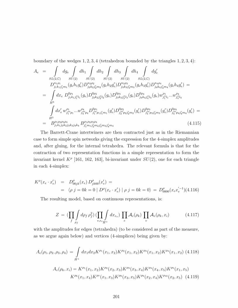
boundary of the wedges 1, 2, 3, 4 (tetrahedron bounded by the triangles 1, 2, 3, 4):

Ae =

∫

SL(2,C)

dge

∫

SU(2)

dh1

∫

SU(2)

dh2

∫

SU(2)

dh3

∫

SU(2)

dh4

∫

SL(2,C)

dg′e

Dn1ρ1j1k1j′1m1

(geh1g′e)D

n2ρ2j2k2j′2m2

(geh2g′e)D

n3ρ3j3k3j′3m3

(geh3g′e)D

n4ρ4j4k4j′4m4

(geh4g′e) =

=

∫

H3

dxe D0ρ1j1k1j′′1 l1

(ge)D0ρ2j2k2j′′2 l2

(ge)D0ρ3j3k3j′′3 l3

(ge)D0ρ4j4k4j′′4 l4

(ge)wρ1j′′1 l1

...wρ4j′′4 l4

∫

H3

dx′e wρ1j′′′1 p1

...wρ4j′′′4 p4

D0ρ1j′′′1 p1j′1m1

(g′e)D0ρ2j′′′2 p2j′2m2

(g′e)D0ρ3j′′′3 p3j′3m3

(g′e)D0ρ4j′′′4 p4j′4m4

(g′e) =

= Bρ1ρ2ρ3ρ4j1k1j2k2j3k3j4k4

Bρ1ρ2ρ3ρ4j′1m1j′2m2j′3m3j′4m4

(4.115)

The Barrett-Crane intertwiners are then contracted just as in the Riemannian

case to form simple spin networks giving the expression for the 4-simplex amplitudes

and, after gluing, for the internal tetrahedra. The relevant formula is that for the

contraction of two representation functions in a simple representation to form the

invariant kernel Kρ [161, 162, 163], bi-invariant under SU(2), one for each triangle

in each 4-simplex:

Kρ(xe · x′e) = Dρ00jk(xe)D

ρjk00(x

′e) =

= 〈ρ j = 0k = 0 | Dρ(xe · x′e) | ρ j = 0k = 0〉 = Dρ0000(xex

′−1e ).(4.116)

The resulting model, based on continuous representations, is:

Z = (∏

f

∫

ρf

dρf ρ2f ) (∏

v,ev

∫

H+

dxev)∏

e

Ae(ρk)∏

v

Av(ρk, xi) (4.117)

with the amplitudes for edges (tetrahedra) (to be considered as part of the measure,

as we argue again below) and vertices (4-simplices) being given by:

Ae(ρ1, ρ2, ρ3, ρ4) =

∫

H+

dx1dx2Kρ1(x1, x2)K

ρ2(x1, x2)Kρ3(x1, x2)K

ρ4(x1, x2) (4.118)

Av(ρk, xi) = Kρ1(x1, x2)Kρ2(x2, x3)K

ρ3(x3, x4)Kρ4(x4, x5)K

ρ5(x1, x5)

Kρ6(x1, x4)Kρ7(x1, x3)K

ρ8(x3, x5)Kρ9(x2, x4)K

ρ10(x2, x5) .(4.119)

201

The variables of the model are thus the representations ρ associated to the triangles

of the triangulation (faces of the dual 2-complex), there are ten of them for each 4-

simplex as can be seen from the expression of the vertex amplitude, and the vectors

xi ∈ H+, of which there is one for each of the five tetrahedra in each 4-simplex

amplitude, so that two of them correspond to each interior tetrahedron along which

two different 4-simplices are glued. We will discuss the geometric meaning of all these

variables in the following section. As written, the partition function is divergent, due

to the infinite volume of the Lorentz group (of the hyperboloid), and the immediate

way to avoid this trivial divergence is just to remove one of the integration over x for

each edge and 4-simplex amplitude, or, in other terms, to gauge fix one variable. It

was shown that, after this gauge fixing is performed, the resulting partition function

(for fixed triangulation) is finite [189, 188].

The functions K appearing in these amplitudes have the explicit expression:

Kρk(xi, xj) =2 sin(ηijρk/2)

ρk sinh ηij(4.120)

where ηij is the hyperbolic distance between the points xi and xj on the hyperboloid

H+.

The amplitudes describe an interaction among the ρ’s that couples different 4-

simplices and different tetrahedra in the triangulation whenever they share some

triangle, and an interaction among the different tetrahedra in each 4-simplex. In

the presence of boundaries, formed by a certain number of tetrahedra, the partition

function above has to be supplemented by boundary terms given by a function

Cρ1ρ2ρ3ρ4(j1k1)(j2k2)(j3k3)(j4k4)

(x) for each boundary tetrahedron [196], being defined as:

Cρ1ρ2ρ3ρ4(j1k1)(j2k2)(j3k3)(j4k4)

(x) = Dρ100j1k1

(x)Dρ200j2k2

(x)Dρ300j3k3

(x)Dρ400j4k4

(x) (4.121)

where x is a variable in SL(2,C)/SU(2) assigned to each boundary tetrahedron,

Dρi00jiki

(x) is a representation matrix for it in the representation ρi assigned to the

i − th triangle of the tetrahedron, and the matrix elements refer to the canonical

basis of functions on SU(2), where the SU(2) subgroup of the Lorentz group chosen

is the one that leaves invariant the x vector thought of as a vector in R3,1, with basis

202

elements labelled by a representation ji of this SU(2) and a label ki for a vector in

the corresponding representation space.

It is this term that gives rise to the amplitude for internal tetrahedra after the

gluing of two 4-simplices along it (it can be seen as just a half of that amplitude

with the integration over the hyperboloid dropped) [177, 196].

Also, we stress that the partition function above should be understood as just

a term within some sum over triangulations or over 2-complexes to be defined, for

example, by a group field theory formalism. Only this sum would restore the full

dynamical content of the quantum gravity theory.

Let us now describe the classical and quantum geometry of the Barrett-Crane

model, i.e. the geometric meaning of the variables appearing in it, the classical

picture it furnishes, and the quantum version of it. Conceptually, the spin foam

formulation of the quantum geometry of a manifold is more fundamental than the

classical approximation of it one uses, and this classical description should emerge

in an appropriate way only in a semi-classical limit of the model; however, the

derivation of the model from a classical theory helps in understanding the way it

encodes geometric information both at the classical and quantum level, even before

this emergence is properly understood.

4.7.1 Geometric meaning of the variables of the model

In this part, we describe the physical-geometrical content of the mathematical vari-

ables appearing in the model. We summarize and collect many known facts and

show how the resulting picture that of a discrete piecewise flat space-time, whose

geometry is described by a first order Regge calculus action (as we then explain in

the next section), in order to explain the physical intuition on which the rest of our

work is based.

The variables of the model are the irreducible representations ρ’s, associated to

each face of the 2-complex, and the x variables, associated to each edge, one for

each of the two vertices it links, as we discussed above.

Consider the ρ variables. They result from the assignment of bivector operators

to each face of the 2-complex, in turn coming from the assignment of bivectors to

the triangles dual to them. Given these bivectors, the classical expression for the

203

area of the triangles is, as we have already discussed: A2t = Bt · Bt = BIJ

t BtIJ ,

and this, after the geometric quantization procedure outlined above, translates into:

A2t = −C1 = −JIJ(ρt)JIJ(ρt) = ρ2t + 1 > 0[110, 111]. Thus the ρ’s determine the

areas of the triangles of the simplicial manifold dual to the 2-complex. The same

result, here obtained by geometric quantization of the bivector field, can also be

confirmed by a direct canonical analysis of the resulting quantum theory, studying

the spectrum of the area operator acting on the simple spin network states that

constitute the boundary of the spin foam, and that represent the quantum states

of the theory. We describe all this in the following. Moreover, from the sign of the

(square of the) areas above, it follows that all the triangles in the model are spacelike,

i.e. their corresponding bivectors are timelike, and consequently all the tetrahedra of

the manifold are spacelike as well, being constituted by spacelike triangles only[111].

As a confirmation, one may note that we have chosen a particular intertwiner -the

simple or Barrett-Crane intertwiner- between simple representations such that it de-

composes into only continuous simple representations, which translates in algebraic

language to the fact that timelike bivectors add up to timelike bivectors. Clearly,

also this sign property of the areas can be confirmed by a canonical analysis.

Consider now the x variables. They have the natural interpretation of normals to

the tetrahedra of the manifold, and the tetrahedra being spacelike, they have values

in H+, i.e. they are timelike vectors in R3,1[165, 208]. The reason for them being in

R3,1 is easily explained. The Barrett-Crane model corresponds to a simplicial mani-

fold, and more precisely to a piecewise flat manifold, i.e patches (the 4-simplices) of

flat space-time glued together along their common tetrahedra[43]. To each flat patch

or 4-simplex (a piece of R3,1) is attached a local reference frame. In other words,

we are using the equivalence principle, replacing the usual space-time points by the

4-simplices: at each 4-simplex, there exists a reference frame in which the space-time

is locally flat. This explains why the normals to the tetrahedra are vectors in R3,1

and also why there are two different normals for each tetrahedron: they are the same

vector seen in two different reference frames. How does the curvature of spacetime

enter the game? Having a curved space-time means that these reference frames are

not identical: we need a non-trivial connection to rotate from one to another (see

also [195]). In this sense, the non-flatness of spacetime resides in the tetrahedra, in

the fact that there are two normals x, y ∈ H+ attached to each tetrahedron, one

204

for each 4-simplex to which the tetrahedron belongs. The (discrete) connection is

uniquely defined, up to elements of the SU(2) subgroup that leaves invariant the

normal vector on which the connection acts, by the Lorentz transformation g rotat-

ing from one of these normals to the other (g · x = y): it is a pure boost connection

mapping two points in H+ into one another1. Thus, the association of two variables

x and y to each edge (tetrahedron) of the 2-complex (triangulation) is the associa-

tion of a connection variable g to the same edge (tetrahedron) (this is of course the

connection variable associated to the edges, and then constrained by the simplicity

constraints, that is used in all the various derivations of the Barrett-Crane model

[135, 136, 134, 167, 157, 177, 196, 195]). From the product of connection variables

around a closed loop in the dual complex, e.g. the boundary of a face dual to a

triangle, one obtains a measure of the curvature associated to that triangle, just as

in traditional simplicial formulations of gravity (i.e. Regge calculus) or in lattice

gauge theory. This set of variables, connections on links and areas on faces, is the

discrete analogue of the set of continuous variables (B(x), A(x)) of the Plebanski

formulation of gravity.

Of course, we have a local Lorentz invariance at each “manifold point” i.e each 4-

simplex. Mathematically, it corresponds to the Lorentz invariance of the amplitude

associated to the 4-simplex. Physically, it says that the five normals (xA, xB, . . . , xE)

to the five tetrahedra of a given 4-simplex are given up to a global Lorentz trans-

formation: (xA, xB, . . . , xE) is equivalent to (g · xA, g · xB, . . . , g · xE). This is also

saying that the local reference frame associated to each 4-simplex is given up to

a Lorentz transformation, as usual. Now, given two adjacent 4-simplices, one can

rotate one of the two in order to get matching normals on the common tetrahedron.

If it is possible to rotate the 4-simplices to get matching normals everywhere, then

the (discrete) connection would be trivial everywhere (i.e. the identity transfor-

mation) and we would get the equivalent of a classically flat space-time. However,

unlike in 3 dimensions where we have only one normal attached to each triangle, in

4 dimensions, we do not want only flat space-times and the “all matching normals”

configuration is only one particular configuration among the admissible ones in the

1The reconstruction of a (discrete) connection or parallel transport from the two normals associ-

ated to each tetrahedron was also discussed in [195] in the context of the Riemannian Barrett-Crane

model.

205

Barrett-Crane model.

The presence of such Lorentz invariance shows that the true physical variables

of the model are indeed pairs of x vectors and not the vectors themselves. One may

use this invariance to fix one of the vectors in each 4-simplex and to express then

the others with respect to this fixed one; in other words the geometric variables

of the model, for each vertex (4-simplex) are the hyperbolic distances between two

vectors corresponding to two tetrahedra in the 4-simplex, measured in the hyper-

boloid H+, i.e. the variables η appearing in the formula (4.120). These in turn have

the interpretation, in a simplicial context, of being the dihedral angles between two

tetrahedra sharing a triangle, up to a sign depending on whether we are dealing

with external or internal angles, in a Lorentzian context (see [197]). These angles

may also be seen as the counterpart of a connection variable inside each 4-simplex.

To sum up the classical geometry underlying the Barrett-Crane model, we have

patches (4-simplices) of flat spaces glued together into a curved space. This cur-

vature is introduced through the change of frame associated to each patch, which

can be identified with the change of time normal on the common boundary (tetra-

hedron) of two patches. Now a last point is the size of the flat space patches, or

in other words the (space-time) volume of a fixed 4-simplex in term of the 10 ρ

representations defining it. This volume can be obtained as the wedge product of

the bivectors associated to two (opposite) triangles − not sharing a common edge

− of the 4-simplex, which reads:

V(4) =1

30

∑

t,t′

1

4!ǫIJKLsgn(t, t

′)BIJt BKL

t′ (4.122)

where (t, t′) are couples of triangles of the 4-simplex and sgn(t, t′) register their

relative orientations. After quantization, the B field are replaced by the generators

J and this formula becomes:

V(4) =1

30

∑

t,t′

1

4!ǫIJKLsign(t, t

′)JIJt JKL

t′ . (4.123)

There is another formula to define the volume, which can be seen as more suitable

in our framework in which we use explicitely the (time) normals to the tetrahedra:

(V(4))3 =1

4!ǫabcdNa ∧Nb ∧Nc ∧Nd (4.124)

206

where is the oriented normal with norm |Ni| = v(3)i the 3-volume of the corresponding

tetrahedron (more on the 4-volume operator in the Barrett-Crane model can be

found in [159]).

4.7.2 Simplicial classical theory underlying the model

Thus the classical counterpart of the quantum geometry of the Barrett-Crane model,

or in other words the classical description of the geometry of spacetime that one can

reconstruct at first from the data encoded in the spin foam, is a simplicial geometry

described by two sets of variables, both associated to the triangles in the manifold,

being the areas of the triangles themselves and the dihedral angles between the two

normals to the two tetrahedra sharing each triangle. A classical simplicial action

that makes use of such variables exists and it is given by the traditional Regge

calculus action for gravity. However, in the traditional second-order formulation of

Regge calculus both the areas and the dihedral angles are thought of as functions

of the edge lengths, which are the truly fundamental variables of the theory. In

the present case, on the other hand, no variable corresponding to the edge length is

present in the model and both the dihedral angles and the areas of triangles have to

be seen as fundamental variables. Therefore the underlying classical theory for the

Barrett-Crane model is a first order formulation of Regge Calculus based on angles

and areas.

A formulation of first order Regge calculus was proposed by Barrett [198] in the

Riemannian case based on the action:

S(l, θ) =∑

t

At(l) ǫt =∑

t

At(l) (2π −∑

σ(t)

θt(σ)) (4.125)

where the areas At of the triangles t are supposed to be functions of the edge lengths

l, ǫt is the deficit angle associated to the triangle t (the simplicial measure of the

curvature) and θt(σ) is the dihedral angle associated to the triangle t in the 4-simplex

σ(t) containing it. The dihedral angles θ, being independent variables, are required

to determine, for each 4-simplex, a unique simplicial metric, a priori different from

the one obtained by means of the edge lengths (actually, unless they satisfy this

constraint, the ten numbers θ’s can not be considered dihedral angles of any 4-

simplex, so we admit a slight language abuse here). Analytically, this is expressed

207

by the so-called Schlafli identity:

∑

t

At dθt = 0. (4.126)

The variations of this action are to be performed constraining the angles to satisfy

such a requirement, and result in a proportionality between the areas of the triangles

computed from the edge lengths and those computed from the dihedral angles:

At(l) ∝ At(θ). (4.127)

The meaning of this constraint is then to assure the agreement of the geometry

determined by the edge lengths and of that determined by the dihedral angles,

and can be considered as the discrete analogue of the “compatibility condition”

between the B field and the connection, basically the metricity condition for the

connection, in the continuum Plebanski formulation of gravity. Note, however, that

this agreement is required to exist at the level of the areas only. This constraint may

also be implemented using a Lagrange multiplier and thus leaving the variation of

the action unconstrained (see [198]). In this case, the full action assumes the form:

S =∑

t

At(l) ǫt +∑

σ

λσ detΓij(θ), (4.128)

where λσ is a Lagrange multiplier enforcing the mentioned constraint for each 4-

simplex, and the constraint itself is expressed as the vanishing of the determinant of

the matrix Γij = − cos θij = − cos (xi · xj), where the x’s variables are the normals

to the tetrahedra in the 4-simplex introduced above.

The main difference with the situation in the Barrett-Crane model is that, in

this last case, the areas are not to be considered as functions of the edge lengths, but

independent variables. The relationship with the dihedral angles, however, remains

the same, and this same first order action is the one to be considered as somehow

“hidden” in the spin foam model. We will discuss more the issue of the simplicial

geometry and of the classical action hidden in the Barrett-Crane model amplitudes,

and of its variation, when dealing with the Lorentzian case.

We point out that other formulations of first order Regge Calculus exist, with dif-

ferent (but related) choices for the fundamental variables of the theory [160][199][200].

208

Also, the idea of using the areas as fundamental variables was put forward at first in

[73] and then studied in [201][202]. The possibility of describing simplicial geometry

only in terms of areas of triangles, inverting the relation between edge lengths and

areas and thus expressing all geometric quantities (including the dihedral angles) in

terms of the latter, was analysed in [203][204][41].

4.7.3 Quantum geometry: quantum states on the bound-

aries and quantum amplitudes

From this classical geometry of the Barrett-Crane model, it is easier to understand

the quantum geometry defined in terms of (simple) spin networks geometry states.

Similarly to the Ponzano-Regge case, the boundary states are Lorentz invariant

functionals of both a boundary connection and the normals on the boundary [205]

and a basis of the resulting Hilbert space is given by the simple spin networks.

More precisely, let us consider a (coloured) spin foam with boundary. The bound-

ary will be made of 4-valent vertices glued with each other into an oriented graph.

Such structure is dual to a 3d triangulated manifold. Each edge of the graph is

labelled by a (face) representation ρ and each vertex corresponds to a (simple) in-

tertwiner between the four incident representations. On each edge e, we can put a

group element ge which will correspond to the boundary connection [196] and we

can decompose the simple intertwiner such that a ”normal” xv ∈ H+ lives at each

vertex v [205].

That way, the boundary state is defined by a Lorentz invariant functional

φ(ge, xv) = φ(k−1s(e)gekt(e), kv.xv) for all kv ∈ SL(2,C) (4.129)

where s(e) and t(e) are respectively the source vertex and the target vertex of the

oriented edge e. This imposes an SU(2) invariance at each vertex v once we have

fixed the normal xv. One should go further and impose an SU(2) invariance for each

edge incident to the vertex in order to impose the simplicity constraints [205]. One

endows this space of functionals with the SL(2,C) Haar measure:

µ(φ) =

∫

SL(2,C)E

dge φ∗(ge, xv)φ(ge, xv). (4.130)

209

x

x

x

1

2

3

g

g

g

g

g

g

1

2

3

4

5

6

ρ

ρ

ρ

ρ

ρ

ρ

1

2

3

4

5

6

Figure 4.11: A (closed) Lorentz spin network

This measure is independent of the choice for the xv due to the gauge invariance

(4.129). Then an orthonormal basis of the Hilbert space of L2 functions is given by

the simple spin networks :

sρe(ge, xv) =∏

e

Kρe(xs(e), ge.xt(e)) =∏

e

〈ρexs(e)(j = 0)|ge|ρext(e)(j = 0)〉, (4.131)

where | ρx(j = 0)〉 is the vector of the ρ representation invariant under SU(2)x (the

SU(2) subgroup leaving the vector x invariant). The general notation is | ρxjm〉for the vector |m〉 in the SU(2) representation space V j in the decomposition Rρ =

⊕jVj(x) of the SL(2,C) representation ρ into representations of SU(2)x.

We should point out that this same Hilbert space for kinematical states comes

out of the canonical analysis of the (generalised) Hilbert-Palatini action in a explicit

covariant framework. Indeed requiring no anomaly of the diffeomorphism invariance

of the theory, the Dirac brackets, taking into account the second class constraints

(simplicity constraints), of the connection AXi (i is the space index and X is the

internal Lorentz index) and the triad P iX , read [184]:

210

IA, IAD = 0

P, PD = 0

AXi , P

jY D = δji I

XY .

(4.132)

where I projects the Lorentz index X on its boost part, this latter being defined

relatively to the time normal x (which is built from the triad field). One can try to

loop quantize this theory: one would like to consider spin networks of the connection

A (cylindrical functions), but in fact, one needs so-called projected spin networks

which depend on both the connection A and the time normal field [205]. Then it

turns out that quantizing these commutations relations at a finite number of points

(the vertices v of the graph) lead to the imposition of the simplicity constraints at

the vertices and the same space of simple spin networks 4.131 as shown in [185].

The graph, representing the quantum geometry state, then has edges labelled with

SL(2,C) simple representations ρ ≥ 0, which corresponds to an area carried by this

edge given by:

area ∼√

ρ2 + 1. (4.133)

The restriction to a finite number of points is natural from the spin foam viewpoint

since the space-like slices are made of tetrahedra glued together and that these

same tetrahedra are considered as the points of this 3d-slice. This explicit relation

between the spin foam setting and the canonical theory is likely to provide us with

information on the dynamics of gravity in both theories.

We have described up to now closed boundaries. What happens if we deal

with an open boundary? Then one needs to introduce open spin networks. Let us

consider a graph with open ends. At all vertices will still live an H+ element (time

normal). The edges in the interior will be defined as previously: on each edge live

a ρ representation and an SL(2,C) group element. On the exterior edges, we still

have an SL(2,C) representation and a group element, but we introduce some new

label, at the (open) end of the edge, which is a vector in the (edge) representation.

Within its SL(2,C) representation, this vector ve can be defined in an orthonormal

basis by its SU(2) (sub)representation j and its label m witin this representation.

211

Then the overall functional is defined as

sρe,jext,mext(ge, xv) =∏

e∈intKρe(xs(e), ge.xt(e))

∏

e∈ext〈ρexint(e)(j = 0)|ge|ρeve = (je, me)〉,(4.134)

where int(e) is the (interior) vertex of the exterior edge e. The scalar product is

defined by the integration over all ge variables. And we get an orthonormal basis

labelled by ρe, jext, mext.We are then ready to explain the geometry behind the amplitude of the Barrett-

Crane model. There are two different ingredients : the 4-simplex amplitude and the

eye diagram corresponding to the tetrahedron amplitude. The 4-simplex amplitude

defines the dynamics of the space-time; it is to be understood as an operator going

from the Hilbert space of quantum states of a (past) hypersurface to the Hilbert

space of quantum states of a (future) hypersurface obtained from the first one by

a Pachner move corresponding to the 4-simplex. The eye diagram is a statistical

weight which can be understood as the number of quantum states of a tetrahedron

defined by the areas of its 4 triangles. Indeed, as we have discussed in section

(4.2), a (classical) tetrahedron is defined by 6 numbers (the 6 lengths of its edges

as an example) and is not fully determined by the 4 areas of its faces: we miss

the values of the area of the 2 interior parallelograms [118]. This indeterminacy

persists at the quantum level. In fact, at the quantum level we can specify, in

addition to the 4 representations corresponding to the 4 triangle areas, an additional

variable for each tetrahedron as a basis for the space of intertwiners between the four

representations in a decomposition of the 4-valent vertex. However, we are forbidden

to specify a further variable corresponding to the other parallelogram area, by a

kind of indeterminacy relation that forces us to leave it completely undetermined

[118]. More precisely, let us note B1, . . . B4 the bivectors of the four triangles of the

tetrahedron. Then, one can construct the areas Ai = |Bi| of the four triangles, the

intermediate areas Aij = |Bi + Bj | of the internal parallelograms and the volume

squared of the tetrahedron U = B1 · (B2 × B3). When quantizing, the bivectors

become SL(2,C) generators in some representation ρi and A2i become the Casimir

of these representations. As for A2ij, it lives in ρi ⊗ ρj and is diagonal on each

(sub)representation ρij in this tensor product. Such an intermediate representation

defines an intertwiner between all four ρ1, . . . , ρ4. When computing the commutator

212

of two such internal areas one gets, as we already mentioned in section (4.2):

[A212, A

213] = 4U. (4.135)

This way, A212 and A2

13 appear as conjugate variables: if one fixes the value of A12

then A13 is undetermined. This can be understood a purely algebraic level: if one

defines the intertwiner between ρ1, . . . , ρ4 through ρ12, then this intertwiner decom-

poses on a whole range of possible ρ13, without fixing it. Thus, the tetrahedron is

never fully specified: the quantum tetrahedron is a fuzzy tetrahedron, with a fluc-

tuating volume U (U depends on both ρ12 and ρ13). Then the eye diagram basically

measures the number of possible states for a tetrahedron (each corresponding to a

possible choice of the unspecified parameter) that do not correspond to different

configuations in the partition function. This explains why we consider it as part of

the measure in the partition function. This statistical interpretation is well-defined

in the Riemannian case for which the dimension of the space of states is finite, and

for which all the geometric quantization procedure leading to the identification of

the space of states for a quantum tetrahedron was carried out. In the Lorentzian

case, the parameters are continuous and the dimensions become infinite, so that it

is better to think in terms of the connection: we replace the data of the 2 interior

areas by the Lorentz transformation between the frames of the two 4-simplices shar-

ing the tetrahedron, which defines the connection internal to the tetrahedron and is

equivalent to the choice of two H+ elements (time-normals). The eye diagram can

be obtained by integrating over the possible connections (SL(2,C) group elements

relating the two normals attached to the tetrahedron) living at the tetrahedron.

This “eye diagram” weight allows all possible connections, thus it randomizes the

connection and correspondingly the space-time curvature. More precisely, it appears

as the amplitude associated to a connection living at a tetrahedron defined by its four

triangle representations (areas). We are aware that [220] proposed another (natural)

interpretation for another tetrahedron weight in the spin foam amplitude which does

not fit with our point of view. Here, we interpret the eye diagram as a localised

quantum fluctuation corresponding to what we could call a quantum refractive wave.

Refractive waves, as introduced in [206], are a new class of gravitational waves.

They allow a discontinuity in the metric while areas are still well-defined. This area

matching condition is exactly what we have in the Barrett-Crane model: two touch-

213

ing 4-simplices will agree on the four face areas of their common tetrahedron while

disagreeing on its complete geometry (different time normals, different volumes).

Moreover it is this indeterminacy which is responsible for the non-topological char-

acter of the Barrett-Crane model. Indeed, in the topological BF model the weight

associated to the eye diagram, obtained by full contraction of two SO(3, 1) or SO(4)

intertwiners without any restriction on the representations summed over, is simply

(and always) one.

One main difference with the Riemannian Barrett-Crane model is that the degen-

eracy of the quantum Lorentzian 4-simplices is unlikely, at least for what concerns

the group representations used, so that we would not have to consider any contribu-

tion to the amplitude from such 4-simplices. This is due to the Plancherel measure.

A degenerate 4-simplex would have some of its triangles of zero area. However, ρ = 0

has Plancherel measure ρ2 = 0 and equivalently has a zero probability. One can be

more precise and look at one particular triangle area probability graph. As we sim-

ply would like to get an idea of what is happening, to simplify the calculations, one

can suppose the space to be isotropic around the triangle. Then the amplitude for

the area ρ is

A(ρ) = ρ2(

sin(ρθ)

ρ sinh(θ)

)N

θ =1

N(2π − θ0) (4.136)

where N is the number of 4-simplices sharing this same triangle and θ0 is the deficit

angle corresponding to the curvature around the given triangle, θ0 = 0 corresponding

an approximatively flat space-time. First, the amplitude is 0 for ρ = 0. Then, we

see that we have a discrete series of maxima which hints toward the possibility of

generating dynamically a discrete area spectrum. Moreover, this spectrum scales

with the curvature. Nevertheless, there is a big difference of the amplitude of each

extremum, which increases with N i.e when we refine the triangulation. Therefore,

for important N , the most probable area ρ is of order 1 (likely between 1 and 6) and

the other extrema are negligible. This is a reason why it is likely that the relevant

regime will be for plenty of small 4-simplices at small ρ and not in the asymptotical

limit ρ→ ∞.

214

4.7.4 The Barrett-Crane model as a realization of the pro-

jector operator

Now we turn to the interpretation of the amplitudes defined by the Barrett-Crane

model. What kind of transition amplitudes do they represent? We have seen that

a path integral realization can be given, in the relativistic particle case, both for

the projector operator over physical states, thus realizing in a covariant manner the

physical inner product among canonical states, and for the Feynman propagator,

or causal transition amplitude; moreover, we have seen that a similar situation is

present at least formally for quantum gravity. Now we have a model that furnishes a

rigorous construction for a sum-over-histories formulation of quantum gravity. The

issue is then to realize whether we have in our hands a projector operator or a causal

evolution operator.

We will argue that the Barrett-Crane model is a realization of the projection

operator for quantum gravity, as argued also for example in [128] and in [82]. In

[128], in fact, a discretization of the projection operator was proposed, leading to

an expression very close to that provided by spin foam models.

In the 4-dimensional case, for the topology Σ × [0, 1], with Σ compact, using a

regular lattice with spatial sections V and with time spacing ǫ and spatial spacing

l, this would read:

P :=

∫

DN ei∫ 10dt∫

d3xN(x,t)H(x) → Pǫ,l =

∫

DN ei∑1/ǫ

t=0

∑

x∈V ǫ l3 N(x)H(x)

=∏

t

∏

x

+∞∫

−∞

dT ei ǫ l3 T H =

∏

t

∏

x

+∞∫

0

dT(

ei ǫ l3 T H + e−i ǫ l3 T H

)

=∏

t

∏

x

Uǫ,l(t, x). (4.137)

The expression above is then interpreted as a sum over triangulations and the

operators Uǫ,l, being (a sum over) local evolution operators, implement the action of

the projection operator on a given spin network and are identified with the quantum

operators corresponding to given Pachner moves in the spin foam case [128]. The

integral over T is then the analogue of the integral over the algebraic variables in

the spin foam model.

215

More generally, the idea is, we stress it again, to regard the partition function

for a spin foam model as giving the physical inner product between (simple) spin

network states as the action of a projector over kinematical spin network states:

〈Ψ2 | Ψ1〉phys = 〈Ψ2 | P | Ψ1〉kin =∑

∆

λ(∆)Z∆, (4.138)

where the full partition function for the given spin foam model has been split into

a sum over triangulations (or their dual 2-complexes) ∆ of partition functions asso-

ciated with each given one.

Still at a formal level, one may thus give a discretized expression for the pro-

jection operator as a sum over triangulations of projectors associated with each

triangulation. In general one may expect then this projector to have the form:

Z(Ψ1,Ψ2) = kin〈Ψ2 | PH=0 | Ψ1〉kin =

+∞∫

−∞

dTei T∫

dxH(x) =∑

∆

λ(∆)∑

σ

+∞∫

−∞

dTσei Tσ Hσ

=∑

∆

λ(∆)∑

σ

∑

tσ

+∞∫

−∞

dTtσei Ttσ Htσ

=∑

∆

λ(∆)∑

σ

∑

tσ

+∞∫

0

dTtσ(

ei Ttσ Htσ + e− i Ttσ Htσ)

, (4.139)

depending on whether the discretization procedure associates the relevant integral

(i.e. the relevant integration variable T or some analogue of it) to the 4-simplices σ

or more specifically to each triangle tσ within each 4-simplex σ.

To obtain a more conclusive argument for considering a given spin foam model as

realizing the projection over physical states one has however to go beyond this and

try to identify the distinguishing features of the projector operator in the particular

spin foam model under consideration. What are then these distinguishing features?

We have already discussed how the difference between a path integral realization of

the projector operator and a path integral formula for the causal transition ampli-

tude is marked uniquely by the presence in the former of a Z2 symmetry relating

positive and negative lapses (or proper times), both in the relativistic particle case

and in the formal path integral quantization of gravity in the metric formalism. We

216

have also seen this symmetry present in the Ponzano-Regge model, which is the

3-dimensional model corresponding to the 4-dimensional Barrett-Crane one. More-

over, we have also noted that a similar and related Z2 symmetry has to be present

in the Barrett-Crane model as well as a result of the quantization procedure that

originated its construction. The task is then to locate clearly where, in the peculiar

structure of the amplitudes of the model, this symmetry is implemented and how.

Let us come back then to the expression for the Barrett-Crane partition function

4.117. We see that, considering the amplitude for the faces and those for the inter-

nal edges as part of the measure, as we suggest is the most reasonable thing to do,

the model has exactly the form 4.139, since the amplitude for the vertices of the

2-complex, encoding the dynamics of the theory and thus related to the Hamilto-

nian constraint, is given by a product of terms each associated to the triangles in

the 4-simplex dual to the given vertex.

Even more remarkably, the K functions associated with each triangle are given

by a sum of two exponentials with opposite signs (with weighting factors in the

denominators), resembling the structure of the formal discretization given above.

Can we interpret the K functions, because of their structure, as encoding the same

Z2 symmetry in the proper time (or in the lapse) that characterizes the projection

operator? The answer is yes.

Consider in fact that, as we noted above, the symmetry T → −T in the proper

time is the same as the symmetry N → −N in the lapse function, in turn originating

from the symmetry B → −B in the bivector field, that we expect to be present in

the model at the quantum level. A change in the sign of B in our discretized

context corresponds to a change in the orientation of the triangles on the simplicial

manifold, and to a consequent change in the orientation of the tetrahedra. Therefore

we expect the sum over both signs of proper time, assuring the implementation of

the Hamiltonian constraint but also erasing causality requirements from the model,

to be realized in our simplicial model as a sum over both orientations of the triangles

and of the tetrahedra in the manifold. This is indeed what happens.

In fact, let us analyse more closely the Z2 symmetry of the K functions. We

use the unique decomposition of SL(2,C) representation functions of the 1st kind

(our K functions) into representation functions of the 2nd kind (we denote them

217

K±)[162] and we write the K function as

Kρij (xi, xj) =2 sin(ηijρij/2)

ρij sinh ηij=

=ei ηij ρij/2

iρij sinh ηij− e− i ηij ρij/2

iρij sinh ηij=

= Kρij+ (xi, xj) + K

ρij− (xi, xj) =

= Kρij+ (xi, xj) + K

ρij+ (−xi,−xj)

= Kρij+ (xi, xj) + K

ρij+ (xj, xi) =

= Kρij+ (ηij) + K

ρij+ (−ηij), (4.140)

which makes the following alternative expressions of the same Z2 symmetry manifest:

Kρij (xi, xj) = Kρij (ηij) = Kρij (−ηij) = Kρij (−xi,−xj) =

= Kρij (xj , xi) = K−ρij (xi, xj). (4.141)

We see that the symmetry characterizing the projection operator is indeed im-

plemented as a symmetry under the exchange of the arguments of the K functions

associated to each triangle in each 4-simplex (so that the resulting model does not

register any ordering among the tetrahedra in each 4-simplex), or as a symmetry

under the change of sign (orientation) of the two tetrahedra sharing the given tri-

angle (so that the resulting model does not register the orientation of the triangle

itself), and these in turn are equivalent to a change in sign of the hyperbolic distance

between the two points on the upper hyperboloid H+ identified by the vectors nor-

mal to the tetrahedra themselves. Also it is a symmetry between a representation

labelled by ρ and its dual labelled by −ρ. It is also possible to consider negative

hyperbolic distance on the upper hyperboloid H+ as positive distances on the lower

hyperboloid H− = x ∈ R3,1|x · x = 1, x0 < 0 in Minkowski space, so that the

symmetry we are considering is in the way the model uses both the upper and lower

hyperboloids in Minkowski space. Note also the analogy between 4.140, for the

kernels K and (1.8) for the Hadamard Green function for the relativistic particle

(maybe it is possible to make this analogy more precise by studying the quantization

of relativistic particles on the upper hyperboloid H+, but we do not analyze this

possibility in this thesis).

218

It is interesting to note also that the reality and positivity of the partition fuction

[207], a puzzling feature indeed if the model was to represent a sum-over-geometries

realization of a causal transition amplitude, i.e. the matrix elements in a spin

network basis of some (unitary?) evolution operator, is perfectly understandable if

the model represents a path integral realization of the projector operator (it is always

possible to find a basis such that the matrix elements of the projector operator are

real and positive). This symmetry can be traced back exactly to the reality of the

K functions and this in turn can be clearly seen as due to the symmetry worked out

above.

Let us stress finally, and clarify, an important conceptual point. What we have

identified is a symmetry under change of orientation which is present in the quan-

tum amplitudes and makes the spin foam model not sensitive to the orientation of

the various geometric elements of the simplicial manifold. The same situation is

present in 3-dimensions for the Ponzano-Regge and the Turaev-Viro models, and in

4-dimensions for the Riemannian Barrett-Crane model. Of course, in the Rieman-

nian case, no causal interpretation is possible, for the absence of a preferred time

direction and of the notion of light cone and causality itself, therefore in this case

we can just talk of dependence or independence from the orientation and that is all.

In the Lorentzian case, this characterization of the symmetry is still available, of

course, and we can talk of whether the model discriminates between a given orien-

ation and its opposite for triangles, tetrahedra or 4-simplices; however, we argue that

at the fundamental quantum level, in absence of any time variable, there is no other

notion of causality than the notion of ordering and orientation, i.e. that it is the

relative orientation of the various geometric elements, and then the ordering of the

boundary states resuting from this, that generates a causal structure for spacetime.

This explains why we talk of causality when dealing with orientation dependence in

this Lorentzian context.

219

4.8 Asymptotics of the 10j-symbol and connec-

tion with the Regge action

As we have already discussed, the dynamics of quantum states is encoded, in spin

foam models, in the vertex amplitudes, i.e. in the amplitudes associated with 4-

simplices of the triangulation and with vertices of the dual 2-complex. Although

the links with Plebanski actions we have shown and the way these amplitudes are

constructed give support to the hope that they really encode all the dynamical

properties of the gravitational field, we would like a further connection with gravity

to arise in a suitable semi-classical limit of these amplitudes. In particular, we

would like a similar situation to the 3-dimensional case to be verified also in this

4-dimensional one, with the large spin asymptotics of the 10j-symbol giving the

exponential of the Regge action for simplicial gravity as a good approximation to

the quantum amplitude, showing then a clear link with the path integral approach

to quantum gravity.

Let us consider the Riemannian case first (see [125, 126, 209]). The vertex am-

plitude is given by a 10j-symbol defined by the contraction of five Barrett-Crane

intertwiners, one for each tetrahedron in the 4-simplex, and given by the integral

formula (4.19). This integral formula gives us also an integral formula for the evalu-

ation of the (simple spin network corresponding to the) vertex amplitude (analogous

to the integral expression for the vertex amplitude in the Lorentzian Barrett-Crane

model):

Av(j) = (−1)∑

t 2jt

∫

(S3)5

∏

t

Kjt(φt) dx1...dx5

= (−1)∑

t 2jt

∫

(S3)5

∏

t

sin(2jt + 1)φt

sin φtdx1...dx5 (4.142)

where, just as in the Lorentzian case, the x variables are interpreted as normals

to the tetrahedra in the 4-simplex, so that φt = arccosx · y is the dihedral angle

associated to the triangle t common to the tetrahedra with normals x and y, the

kernels K result from the contraction of two representation matrices, the quantities

220

at = 2jt + 1 are the areas of the triangles, and we have neglected a factor 1∆j1

..∆j10

in the denominator, since it does not affect the results to be described.

It is known [207] that the integral above is positive, so we take a rescaling

with parameter N of the ten areas and consider its absolute value only in order to

study its asymptotics for large N . As in the 3-dimensional case, there is a region

in the integration domain where the integrand is divergent, for φt = 0, π, so we

split the integral into two contributions, one corresponding to the “safe” sector of

the integration domain, which we call it I>, i.e. for φt ∈ [ǫ, π − ǫ], with ǫ << 1

and one close to these critical points, i.e. for φt ∈ [0, ǫ] ∪ [π − ǫ, π], corresponding

to degenerate geometries for the 4-simplex, since they correspond to the 4-simplex

being “squeezed” to a 3-dimensional hypersurface, which we call I<.

Consider I> first. Writing the kernels as a sum of exponentials we obtain an

expression of the form:

I> =

∫

(S3)5

∑

σt

f(x1, .., x5)∏

t

ei σt N at φt =

∫

(S3)5

∑

σt

f(x1, .., x5) ei∑

t σt N at φt(4.143)

where σ = ±1 and f(x1, .., x5) =1

∏

t sinφt, and the quantity in the exponential can

be intepreted as an action S(σ, x, a) whose stationary points dominate the integral.

Using the fact that the dihedral angles are constrained to satisfy the Schlafli identity

we mentioned above, the stationary phase analysis of the integral, involving the

variations of the action, in the limit N → ∞ gives as a result [125, 209, 126]:

I> ∼∑

i

1

N92

f(xi)√

H(xi)cos

(

∑

t

N at φt(xi) +π

4s(H(xi))

)

, (4.144)

where the sum is over the statonary points xi of the action S, H(xi) is the deter-

minant of the matrix of second derivatives of S computed at the points xi, s(H) is

the signature of this matrix, and, most important, the resulting action, appearing

in the argument of the cosine, once we have fixed the signs σ to the values given

by the stationary points (these result to be all positive or all negative), is just the

contribution of a single 4-simplex to the Regge calculus action for gravity.

The result then shows that, in this asymptotic limit, the non-degenerate con-

figuration in the spin foam model give a contribution of the order O(N− 92 ) to the

amplitude and with a term proportional to the exponential of the Regge calculus

221

action for simplicial gravity, just as the Ponzano-Regge model in 3-dimensions. This

result was obtained first in [208] and then confirmed recently in [125, 126, 209].

One needs however to worry about the degenerate configurations as well, to see

whether they actually dominate the amplitude or not. In the 3-dimensional case

we have seen that their contribution is of the same order of magnitude as the non-

degenerate ones. In this case, however, the result is different. In fact we obtain, for

the integral I< [125, 209, 126]:

I< ∼ 1

N2

∫

(R3)5

du1..du5∏

t

sin(at | ut1 − ut2 |)| ut1 − ut2 |

(4.145)

so we see that its contribution is of the order O(N−2) so that it tends to dominate

the amplitudes in the asymptotic limit.

This result may be obtained also defining “degenerate spin networks” corre-

sponding to these degenerate configurations and based on the symmetry group of

the hypersurface to which the 4-simplex is confined when degenerate, i.e. the Rie-

mannian group E3, since an appropriate formalism for their evaluation can be defined

in full [126, 209].

This result is, in itself, quite disappointing, since it may imply, if the asymp-

totic approximation to the amplitudes so computed is indeed what describes the

semi-classical limit of the theory, that the Barrett-Crane spin foam model does not

reproduce classical simplicial gravity in the semiclassical limit but it is dominated

only by degenerate geometries.

However, much more work is needed to understand the real implications of this

result, for several reasons: it may well be that classical gravity is not to be obtained

by this method or in the asymptotic limit; recall in fact that the amplitudes have to

be used within a sum over triangulations and it may well be that the semi-classical

limit in this wider context has to be approched and studied by very different methods

than this asymptotic one; moreover, we have argued that the Barrett-Crane model

corresponds in fact to a first order formulation of simplicial gravity, with two sets

of variables, areas and dihedral angles to be treated on equal footing, while the

procedures we described held fixed the areas and considered the contribution of

different dihedral angle configurations to the amplitude; maybe a more symmetric

222

procedure is needed, based on something like a WKB approximation for two sets of

coupled variables.

The Lorentzian case has been studied in details in [209], to which we refer,

and the results are analogous to those described above for the Riemannian. The

degenerate and non-degenerate configurations give the same type of contribution to

the asymptotic limit, and, most important, with the same order of magnitude. The

implication of this result have then still to be understood also in this Lorentzian

context.

223

Chapter 5

The group field theory formulation

of spin foam models in 4d

In this chapter we want to describe in detail how the Barrett-Crane model we have

derived and discussed in the previous chapter can be obtained using the technology of

field theories over group manifolds, in analogy with the group field theory derivation

of the Ponzano-Regge model we have already discussed. We deal with both the

Riemannian and Lorentzian cases, and try to explain more at length the origin of

the simplicial complexes as Feynman graphs of the group field theory; we discuss

the subtleties of this correspondence and whether these simplicial complexes are or

are not simplicial manifolds; finally, we discuss the physical interpretation of the

group field theories from a quantum gravity point of view.1

Matrix models were invented more than 15 years ago to give a precise formulation

of 2d quantum gravity (or “zero-dimensional string theory”) [211, 212, 213, 214,

215]. The group field theories may be seen as a generalization of these matrix

models, where tensors replace matrices as fundamental variables, and as such were

constructed in 3 dimensions by Boulatov [216], whose model gives the Ponzano-

Regge-Turaev-Viro (spin foam) formulation of 3d quantum gravity, as we have seen,

and in 4 dimensions by Ooguri [217], giving the Crane-Yetter spin foam formulation

of 4d BF theory

1For a comparison of this approach to quantization with the canonical one and the spin foam

procedure in the simple case of 2d BF theory, see [210].

224

[67, 68], a quantum topological field theory. It could be expected that imposing

in a proper way the Barrett-Crane constraints in the Ooguri model would give in the

end the Barrett-Crane state sum instead of the Crane-Yetter one, so giving quantum

gravity in 4 dimensions instead of a topological theory. This is indeed the case, as

we will see. The first derivation of the Barrett-Crane model from a field theory over

a group manifold was given in [133], and an alternative one was proposed in [134].

A general formalism for deriving a whole class of spin foam models from a group

field theory was developed in [135, 136], proving the power and versatility of the

formalism itself, and further study on this topic is in [218, 219]. The model of [134]

reproduces exactly the Barrett-Crane state sum in the form given when we derived

it from a lattice gauge theory perspective, while the model in [133] provides an

alternative choice of amplitudes for the edges of the spin foam, and other variations

leading to different choices are possible as we will show.

Before turning to a more detailed description of a field theory giving the Barrett-

Crane state sum, we would like to point out what are the most interesting aspects

of this approach. First of all the purely algebraic and combinatorial nature of the

model, and its background independence, are made manifest, since the field theory

action is defined in terms of integrals over a group of scalar functions of group el-

ements only, while its mode expansions involve only the representation theory of

the group used, and its Feynman graphs (describing “interactions”) require only no-

tions of combinatorial topology to be constructed. Then these Feynman graphs are

interpreted as encoding the geometry of a 4-dimensional (Riemannian) spacetime,

but no geometric notion enters in their definition. The basic tool involved in the

definition of the models is the harmonic analysis of functions on the group, and the

resulting representation theory, so no reference is made to any spacetime geometry

or topology even, and this is why they allow for a fully background independent

formulation of a theory of quantum spacetime. Moreover, this approach permits a

natural implementation of a suitable sum over spin foams, i.e. the key ingredient

missing in the other derivations and necessary for a complete definition of a spin

foam model for 4-dimensional quantum gravity, since in the 4-dimensional case, as

we stressed already, any choice of a fixed triangulation represents a truncation of

the dynamical degrees of freedom of the gravitational field.

225

5.1 General formalism

The fundamental idea of this approach is that one can represent a tetrahedron in 4-

dimensions, to which a state of the quantum theory can be associated, by a function

of four group variables (where the group G is of course the Lorentz group sl in the

Lorentzian case and Spin(4) in the Riemannian) to be thought of as associated to

its four triangular faces. The action is then chosen in such a way to mimic the

combinatorial structure of a simplicial manifold, i.e. with an interaction term given

by a product of five fields since a 4-simplex has five tetrahedra and a 4-simplex can be

interpreted as an elementary interaction of tetrahedra. The kinetic term is of course

quadratic in the fields, as is usual in field theories. These considerations are already

almost enough to write down the models for the group field theory actions giving rise

to the topological models corresponding to BF theory in different dimensions. When

it comes to gravity the situation is more complicated since there are many different

ways of imposing the constraints that reduce BF theory to gravity, as conditions on

the fields in the action; this ambiguity is what originates the different models, all

understandable as different versions of the Barrett-Crane model, that we are going

to discuss.

The field is a (scalar) function of four group elements: φ(g1, g2, g3, g4), that

can be simply written as φ(gi). We may require different symmetry properties on

this field with respect to permutations of its four arguments, i.e. we may require:

φ(g1, g2, g3, g4) = φ(gπ(1), gπ(2), gπ(3), gπ(4)), where π is a generic permutation of (1234)

or an even permutation only, etc. Different choices give rise to different models, as

we will see. We also define group projectors Pg and Ph by means of which we impose

additional conditions on the fields: we impose invariance under the group G (gauge

invariance) applying the projector Pg:

Pg φ(g1, g2, g3, g4) =

∫

G

dg φ(g1g, g2g, g3g, g4g), (5.1)

and invariance under an appropriately chosen subgroup H applying the projector

Ph:

Ph φ(g1, g2, g3, g4) = (∏

i=1..4

∫

H

dhi)φ(g1h1, g2h2, g3h3, g4h4). (5.2)

226

One then defines an action for the field, which in 4 dimensions is a φ5 action, i.e.

of the form S =∫

φ2 + λφ5, where the integral is over the group elements that can

be thought of as representing the triangles of a simplicial complex; more precisely:

S[φ] =1

2

∫

dgidgiφ(gi)K(gi, gi)φ(gi)−λ

5

∫

dgijV(gij)φ(g1j)φ(g2j)φ(g3j)φ(g4j)φ(g5j),(5.3)

with φ(g1j) = φ(g12, g13, g14, g15) and so on. K and V are the kinetic operator (whose

inverse, in the space of gauge invariant fields, is the propagator of the theory) and

the vertex (or potential) operator respectively. Alternatively, one can expand the

field in modes, i.e. apply the rules of the harmonic analysis of functions on groups,

and re write the action in terms of these modes, so that a conjugate expression of

the kinetic and potential operators has to be used. The modes of the field will be

functions of four group representations, instead of the four group elements.

The partition function of the theory is given, as in the usual quantum field theory

literature, by an integral over the field values of the exponential of the action, and

can be re-expressed in terms of its Feynman graphs (as an expansions in powers of

λ) as:

Z =

∫

Dφ e−S[φ] =∑

Γ

λv[Γ]

5!v v! sym[Γ]Z[Γ], (5.4)

where v[Γ] and sym[Γ] are the number of vertices and the order of symmetries

(number of automorphisms) of the Feynman graph Γ. This last number sym[Γ] can

be shown [219] to be: sym[Γ, v] = 25 v/2 · (5 v/2)!.So we are interested in finding the form of the amplitude for a generic Feynman

graph, i.e. the Feynman rules of the theory. We will see that this amplitude for

each Feynman graph is exactly the partition function for fixed triangulation that we

have derived from a lattice gauge theoretic approach above, for a triangulation to

be put in correspondence with a given interaction graph of the group field theory.

In order to understand how this correspondence is to be found, let us analyse more

closely the construction of the Feynman graphs.

The propagator (see figure 5.1) can be represented by four straight parallel lines,

representing the four arguments of the field or of its modes, and has a group variable

or a group representation) at the two ends of each line, while the vertex operator

227

Figure 5.1: The propagator of the theory; each of the four strands carries a (simple)

representation of the group and the box stands for a symmetrization of the four

arguments, i.e. for a sum over given permutations of the ordering of the arguments

Figure 5.2: The vertex of the theory; it has the combinatorial structure of a 4-simplex

and has a (simple) representation of the group at each open end

228

Figure 5.3: The construction of a Feynman graph of the theory, connecting a prop-

agator with a vertex

( 5.8) (see figure 5.2 ) has the combinatorial structure (given by the way it pairs the

arguments of the fields) of a 4-simplex, with 5 vertices and 4 lines coming out of

each of them (five tetrahedra-propagators with four triangles-lines each), again with

a group variable or group representation at the two ends of each line. Everywhere at

the open ends of propagators and vertices are the four group variables that are the

arguments of the field. All the possible Feynman graphs are obtained (see figure 5.3)

connecting a number of vertices with the propagators, constructing in this way what

is called a “fat graph” for each possible permutation of the lines in the propagator.

Each of the strands of a propagator is connected to a strand in one of the five

“open sites” of the vertex, in such a way that the orientations in vertices and prop-

agators match. Moreover, because of the symmetry of the field, each propagator

really corresponds to many different terms given by the different ways in which its

four carried indices can be permutated. Which are these possible ways depends of

course by the symmetries under permutations we have imposed on the field, so that

all possible permutations appear in the propagator, or only all the even ones, etc.

In this way, the sum over Feynman graphs Γ can be re-written as a sum over fat

graphs γ, with an amplitude for each fat graph, as:

Z(λ) = 1 +∑

γ

w(γ) · λv(γ) Z(γ), (5.5)

229

where w(γ) = l(γ)

v(γ)!·(5!v(γ) ·(4!)e(γ)−v(γ) , w(γ) is the number of inequivalent ways of la-

belling the vertices of γ with v(γ) symbols and e(γ) is the number of links in γ.

Now, each strand of the fat graph can go through several propagators and several

vertices, and at the end closes on itself, and consequently forms a cycle. This cycle

is labelled (in “momentum space”) by the representation assigned to the strand that

encoles it. The abstract object formed by these cycles, the edges and the vertices is a

2-complex, moreover, since each face (cycle) is labelled by a representation of G, this

is a labelled 2-complex, i.e. a spin foam. So we see that there is a 1-1 correspondence

between the Feynman graphs of our field theory and spin foams. This means that

the sum in ( 5.4) can be interpreted as a sum over spin foams (labelled 2-complexes),

the amplitude Z(Γ) as an amplitude for each spin foam, and the partition function

itself defines a spin foam model. In turn, each 2-complex can be thought of as dual

to a triangulation, i.e. a simplicial complex. In general it is not true that a simplicial

complex is determined by the dual 2-skeleton, but it is true in this case since the

complex is obtained by gluing of codimension-1 faces of simplices. Knowing this,

we can interpret the vertices as referring to 4-simplices, and the propagators to

the tetrahedra they share, an interpretation that we had anticipated but that we

now see as justified. At this stage attention must be paid to the properties of the

simplicial complexes that are in correspondence with the Feynman graphs. When

working with a fixed triangulation, one could always assume the properties wanted

for it, in particular it was possible to assume that the complex would satisfy the

conditions necessary to make it a proper manifold. Now, the theory itself generates

the simplicial complexes we work with as a sum over Feynman graphs as we have

just said and we have to check whether these conditions are fulfilled or not.

Before discussing these manifold conditions, let us say more about which kind of

complexes arise in the expansion. First of all, if we define the orientation of a vertex

of the 2-complex as an ordering of its adjacent edges up to even permutations,

and an orientation of the edges as the one induced by the vertex, we see that

the orientation of two vertices linked by an edge is consistent only if the edge is

induced opposite orientation by the two vertices, and we can define a 2-complex

orientable if it admits a consistent orientation of all its vertices. Equivalently, a

2-complex is orientable if all its loops are even. In particular, a 2-complex dual to a

traingulation of an orientable manifold is orientable. Given this definition, it is easy

230

to check [133] that if we require the field to be invariant under even permutations

only of its arguments, the propagators above contain odd permutations only, while

the pairing of strands determines always an odd permutation. If we then consider

a loop of edges in a Feynman graph, we cross an equal number of vertices and

edges, and therefore the strands undergo an even number of odd permutations.

This means that for each loop we have always an even permutation and the 2-

complex is orientable. Therefore the field theory based on a field invariant under

even permutations only generates a sum over orientable 2-complexes only. this is

not true for other choices pf symmetries for the field. Second, it is also easy to check

that the pairing of lines in vertices and propagators, taken into account the different

possibilities involved in each propagator, originates not only all the triangulations

of a given topology obtained with a given number of top-dimensional simplices, but

also all the triangulations of all the possible topologies, indeed corresponding to all

the possible pairing of lines, i.e. to all the possible gluing of triangles. Therefore,

the group field theory generates a sum over topologies as well as a sum over different

triangulations of the same topology, so gives rise to a fully background independent

theory of spacetime.

Let us now turn to the manifold conditions [218, 219]. The condition for a space

M to be a manifold is that each point in it has to have a closed neighbourhood

homeomorphic to a disk D4 (in 4-dimensions). There is also another way to formu-

late the same condition: consider the space M∂ (closed with boundary) constructed

by gluing the polyhedra obtained by removing the open star of the original vertices,

then the condition is thatM is a manifold iff the boundary ofM∂ is a disjoint union

of 3-spheres.

There is nothing to check for the point in the interior of the simplices or on tetra-

hedra. As a consequence, in dimensions 2 and 3 the condition is always fulfilled.

In dimension four, we have to check this condition on the barycenters of triangles

and edges. A complete characterization of these condition in terms of conditions on

the fat graphs can be given [218, 219] and it can be shown that in the expansion

generated by the group field theory not all the fat graphs correspond to simplicial

manifold, but some of them correspond to simplicial manifolds with conical singu-

larities. Whether the field theory has then to be suitably modified so to incorporate

only simplicial manifold, or whether the inclusion of conifolds has to be considered

231

as a feature and not a problem of this approach, is at present not understood. On

this see also [230, 231].

5.2 Riemannian group field theories

We present now different versions of the Riemannian Barrett-Crane model, existing

in the literature, and as obtained by group field theory, and then give the most

general structure of this kind of model. These different versions arise because of the

non-trivial interplay between the two projectors Pg and Ph we defined above.

The starting point is the field φ(g1, g2, g3, g4). One can then impose on it the

projector Ph making it a field over four copies of the homogeneous space G/H

and then impose gauge invariance by means of the projector Pg, so that the basic

object of the theory is the field: PgPhφ(g1, g2, g3, g4). We recall that the projector Ph

imposes invariance under a given subgroup H of G, and restricts the representations

involved in these models to be the simple (class 1) representations with respect to

this subgroup, while the projector Pg imposes gauge invariance (invariance under the

full group G). Alternatively, one can decide to work with gauge invariant fields from

the beginning, having as basic object the field Pgφ(g1, g2, g3, g4). On this field one

can then impose further projectors. Another choice then is involved: we can decide

to impose more projectors and in different combinations in the kinetic and in the

potential terms in the action. We will see that the models existing in the literature all

work with gauge invariant fields as basic objects, but differ in the way they impose

further projectors in the kinetic and potential terms. These difference are more

manifest in the conjugate representation of the fields in terms of representations of

the group, i.e. using their mode expansion.

5.2.1 The Perez-Rovelli version of the Riemannian Barrett-

Crane model

A first possibility is to work with gauge invariant fields Pgφ, and then impose the

combination of projectors PgPh in the interaction term of the action only.

232

The action is then:

S[φ] =1

2

∫

dg1...dg4 [Pgφ(g1, g2, g3, g4)]2 +

+λ

5!

∫

dg1...dg10 [PgPhPgφ(g1, g2, g3, g4)] [PgPhPgφ(g4, g5, g6, g7)]

+ [PgPhPgφ(g7, g3, g8, g9)] [PgPhPgφ(g9, g6, g2, g10)] [PgPhφ(g10, g8, g5, g1)] , .(5.6)

The removal of the combination of projectors PgPh would lead to a model directly

analogous to the Boulatov model giving the Ponzano-Regge spin foam mdoel, called

Ooguri model, and corresponding to 4-dimensional BF theory. We work here with

the field φ, but it is clear that one could redefine φ′ = Pgφ without affecting the

result, but changing only the expression for kinetic and potential operators. Using

the notation anticipated above, the kinetic term in “coordinate space” is given by:

K(gi, gi) =∑

σ

∫

dγ∏

i

δ(

gi γ g−1σ(i)

)

, (5.7)

which corresponds to a projector in to the space of gauge invariant fields, and is

such that it is equal to its inverse, so that the propagator is K itself. In the formula

above the product is over the four arguments of the field and the sum is over the

possible even permutations of them. If we had used the redefinition φ → φ′ the

kinetic operator would have been only a product of deltas without any integral over

G = SO(4).

The vertex operator is:

V(gij) =1

5!

∫

dβidβidhij∏

i<j

δ(

g−1ji βihijβ

−1i βjhjiβ

−1j gij

)

(5.8)

where β and β are SO(4) integration variables, and hij ∈ SO(3). Again the product

is over the arguments of the fields entering in the interaction term.

The amplitude for a Feynman graph is then given by a product of interaction

terms V(gij), one for each vertex of the graph, connected by propagators P(gi, gi) =

K, one for each edge of the graph, with an integral over the original group elements

common to both kinetic and potential terms. Doing this for a generic Feynman

graph, using the 2-complex corresponding to it, and recalling the correspondence

between this and a simplicial complex, it is easy to check that this model gives an

233

amplitude identical to the one defined in section (4.4) for the Barrett-Crane model,

i.e. a delta function of a product of group elements assigned to the boundary links

of each face of the 2-complex, with the same projections inserted, meant to impose

the constraints that reduce BF theory to gravity. This fact is even more evident in

the momentum formulation of the model

Because of the Peter-Weyl theorem we can expand any L2(G) function φ(g) over

the group G = SO(4) in terms of matrices DΛαβ(g) of the irreducible representations

Λ of SO(4) (repeated indices are summed over), so we can expand our basic field

Pgφ(g1, g2, g3, g4) as:

Pgφ(g1, g2, g3, g4) =∑

J1,J2,J3,J4Λ

φJ1J2J3J4α1β1α2β2α3β3α4β4

DJ1β1γ1

(g1)...DJ4β4γ4

(g4)CJ1J2J3J4Λγ1γ2γ3γ4 CJ1J2J3J4Λ

α1α2α3α4.(5.9)

and then redefine the field components as:

ΦJ1J2J3J4Λβ1β2β3β4

≡ φJ1J2J3J4α1β1α2β2α3β3α4β4

CJ1J2J3J4Λα1α2α3α4

, (5.10)

where the C’s are SO(4) intertwiners.

Inserting this expansion into the action, we have for the kinetic term in the

action:

K =∑

J1,J2,J3,J4,Λ

ΦJ1J2J3J4Λα1α2α3α4

ΦJ1J2J3J4Λβ1β2β3β4

(∆J1∆J2∆J3∆J4)−1 δα1β1 ...δα1β1, (5.11)

and for the potential term:

V =1

5

∑

J

∑

Λ

ΦJ1J2J3J4Λ1α1α2α3α4

ΦJ4J5J6J7Λ2α4α5α6α7

ΦJ7J3J8J9Λ3α7α3α8α9

ΦJ9J6J2J10Λ4α9α6α2α10

ΦJ10J8J5J1Λ5α10α8α5α1

(∆J1...∆J10)−2 BBC

J1...J10, (5.12)

where BBC is the Barrett-Crane amplitude given by a product of five fully contracted

Barrett-Crane intertwiners. From these expressions we can read off the formulae for

the propagator

Pα1β1...α4β4 = δα1β1...δα4β4 (∆J1∆J2∆J3∆J4) (5.13)

and for the vertex amplitude given by the Barrett-Crane amplitude, as we said, with

the coefficient appearing in the fomula above. Using these formulae, and taking into

234

account the extra sum over the Λs, labeling the intertwiners of the 4 representations

J1, J2, J3, J4, we have for each Feynman graph J the amplitude:

Z(J) =∑

J

∏

f

∆Jf

∏

e

∆1234(

∆Je1∆Je2

∆Je3∆Je4

)

∏

v

BBCv (5.14)

where ∆1234 is the number of possible intertwiner between the representations J1, J2, J3, J4,

the sum is over the simple (because of the projection operators Ph imposed above)

representations of SO(4) and the products are over the faces, edges and vertices

of the Feynman graph, or equivalently over the faces, edges and vertices of the

corresponding spin foam. Moreover, we see that we have obtained precisely the

Barrett-Crane state sum model as derived in section (4.4), with a precise match-

ing of the face, edge and vertex amplitudes; this is the Perez-Rovelli version of the

Barrett-Crane model, as obtained in [134].

We close by noting that the same kind of action, but with the group used being

SO(D), the field being a function of D group variables, and the projector Ph impos-

ing invariance under an SO(D−1) subgroup, would result in the higher-dimensional

generalization of the Riemannian Barrett-Crane model we have sketched in section

(4.4.3).

5.2.2 The DePietri-Freidel-Krasnov-Rovelli version of the

Barrett-Crane model

Instead of imposing the combination of projectors Pg and Ph only in the interaction

term, we can impose it also in the kinetic term, using the combination PhPg, defining

the action to be:

S[φ] =1

2

∫

dg1...dg4 [PhPgφ(g1, g2, g3, g4)]2 +

+λ

5!

∫

dg1...dg10 [PhPgφ(g1, g2, g3, g4)] [PhPgφ(g4, g5, g6, g7)]

× [PhPgφ(g7, g3, g8, g9)] [PhPgφ(g9, g6, g2, g10)] [PhPgφ(g10, g8, g5, g1)] , .(5.15)

In this case one can see that the kinetic operator of the theory is given, in

coordinate space, by:

K(gi, gi) =∑

σ

∫

dhidγdγ∏

i

δ(

gi γ hi γ g−1σ(i)

)

, (5.16)

235

while the vertex is:

V(gij) =1

5!

∫

dβidβidhij∏

i<j

δ(

g−1ji βihijβ

−1i βjhjiβ

−1j gij

)

. (5.17)

Now the kinetic operator is not a projector anymore, and therefore the definition

of its inverse in coordinate space, giving the propagator of the theory, is much more

complicated. The analysis is much simpler in momentum space.

The field, including the projectors, can be expanded in modes, again using the

Peter-Weyl theorem, as follows:

PhPgφ(g1, g2, g3, g4) =∑

J1,J2,J3,J4,Λ

φJ1J2J3J4α1β1α2β2α3β3α4β4

DJ1β1γ1

(g1)...DJ4β4γ4

(g4)CJ1J2J3J4Λγ1γ2γ3γ4

CJ1J2J3J4Λδ1δ2δ3δ4

wJ1δ1wJ1

α1...wJ4

δ4wJ4

α4=

=∑

J1,J2,J3,J4,Λ

ΦJ1J2J3J4β1β2β3β4

DJ1β1γ1

(g1)...DJ4β4γ4

(g4)CJ1J2J3J4Λγ1γ2γ3γ4 (∆1 ∆2∆3∆4)

− 14 . (5.18)

with the evident redefinition of the field.

Using this expansion, the kinetic term in the action assumes the form:

K =∑

J1,J2,J3,J4,Λ

ΦJ1J2J3J4α1α2α3α4

ΦJ1J2J3J4β1β2β3β4

(∆J1∆J2∆J3∆J4)− 3

2 ∆1234 δα1β1...δα4β4, (5.19)

and the potential term is:

V =1

5!

∑

J

ΦJ1J2J3J4α1α2α3α4

ΦJ4J5J6J7α4α5α6α7

ΦJ7J3J8J9α7α3α8α9

ΦJ9J6J2J10α9α6α2α10

ΦJ10J8J5J1α10α8α5α1

(∆J1 ...∆J10)− 3

2 BBCJ1...J10

. (5.20)

The propagator can then be read off immediately from the expression of the

kinetic term:

P = (∆J1∆J2∆J3∆J4)3/2 ∆−1

1234 δα1β1 ...δα4β4 , (5.21)

Building up the amplitudes for each Feynman graph as usual, the result is:

Z(F ) =∑

J

∏

f

∆Jf

∏

e

1

∆1234

∏

v

BBCv . (5.22)

The function ∆1234 can be thought of as the norm square of the Barrett-Crane

intertwiners between the representations J1, J2, J3, J4, since BJ1J2J3J4γ1γ2γ3γ4

BJ1J2J3J4γ1γ2γ3γ4

=

236

∆1234; therefore this model, as it is easy to check, can be interpreted as having

no edge amplitude at all, but simply using normalized Barrett-Crane intertwiners

wherever they are involved in the definition of the vertex amplitudes.

We note, however, that no lattice gauge theory derivation of this model is known,

due to the difficulties mentioned in section (4.5.2).

5.2.3 Convergence properties and spin dominance

Let us discuss now some properties of the models we have just derived. Not much is

understood about the properties of the sum over 2-complexes; it is almost certainly

a divergent sum, but because it is interpreted as a perturbative expansion of a field

theory partition function, this is not surprising nor would it be too upsetting, if it

could be shown that the sum itself is just an asymptotic series of some known and

computable (and possibly meaningful) function. i.e. if it were possible to give it

a non-perturbative definition and meaning. Unfortunately, no result of this kind is

available yet, unlike the 3-dimensional case [138].

Anyway, convergence of the partition function or of the generic transition am-

plitudes, although useful, since it simplifies the technical matters, may well not be

a necessity at all, since when computing expectation values of observables (which

is were physics is) one usually works with expressions like: 〈O〉 = Z(O)Z

=∑

F OA(F )∑

F A(F ),

and the fact that both numerator and denominator diverge may not preclude the

meaningfulness of 〈O〉. Also, if one wants a canonical interpretation of the theory,

one is interested in defining the scalar product between states 〈Ψ | Ψ′〉 where a

normalization by means of a quotient with respect to the modulus of the vacuum

state (partition function in the denominator) is not necessarily to be used, and for

computing this kind of quantities, the well-posedness of the sum over histories defi-

nition of the states and of the scalar product may be necessary. The situation, thus,

is not so clear.

Still from a field theoretic point of view, another attractive possibility would be

that each term of the expansion, i.e. each amplitude for a given Feynman graph,

is either finite or regularizable (made finite). This would imply nothing about the

behaviour of the full partition function, but will be important if the single terms in

the perturbation expansion of the group field theory, i.e. the amplitudes for fixed

237

triangulations, can be given a physical interpretation on their own. For example, if

we interpret them as it is natural as path integral expressions for gravity on a fixed

triangulation, i.e. path integrals for discrete gravity, their finiteness would be quite

remarkable.

Luckily, it is possible to study these issues both analytically and numerically,

thanks to the tools developed in [220, 207], i.e. an efficient algorithm for computing

simple Riemannian spin networks (and thus spin foam amplitudes).

We start from the DePietri-Freidel-Krasnov-Rovelli version of the Barrett-Crane

model. It can be shown numerically that the partition function for fixed trian-

gulation in this version of the model diverges very rapidly even for the simplest

triangulation, i.e. those involving very few vertices. In particular for the simple

case of a 6-vertices triangulation of a 4-sphere, after having imposed a spin cut-off

J , it can be extimated a dvergence of the order O(J23), so spectacularly rapid in-

deed. This divergence is mainly due to the rapid grow of the face amplitudes with

increasing spins, while the 10j-symbols decay in J as O(J−2) and the 4j-symbol

or ∆1234 or “eye diagram” grows as O(J), so there may be a slower grow only for

triangulations which involve many vertices and edges compared to faces; since for

non-degenerate triangulations the number of tetrahedra is always 5/2 times the

number of 4-simplices, it may be possible only for triangulations were a very high

number of 4-simplices share any given triangle. Because of these convergence prop-

erties, the amplitudes are dominated by configurations with extremely high values

of the representations assigned to the triangles, which would naively (but possibly)

correspond to very large areas of these.

In the Perez-Rovelli version, the situation is basically the opposite. Analytically

it can be shown [187] that, for any triangulation of a pseudomanifold (manifold

with possible conical singularities) such that each triangle lies in at least three 4-

simplices, the sum over representations giving the quantum amplitude for the given

triangulation is indeed finite, i.e. convergent. This implies, at least for this (large)

class of triangulations or Feynman graphs, perturbative finiteness to all orders from

the point of view of the group field theory or from the lattice gauge theory point

of view (that we have used to derive this model in section (4.4)) a well defined

partition function for any choice of discretization of the theory. Remarkable and

quite striking. More precisely, the following upper bound for the amplitude Z(J) of

238

an arbitrary 2-complex J was found [187]:

| Z(∆) |≤∏

f∈J

∑

jf

(

∆jf

)−1= (ζ(2)− 1)F∆ ≈ (0.6)F∆ , (5.23)

where the product is over the faces of the 2-complex, the sum is over their associated

representations, ζ is the Riemann zeta function, and F∆ is the total number of faces

in the 2-complex ∆.

Numerical tools can be applied here as well. In this way the covergence can be

confirmed “empirically”. Moreover, the numerical simulations show a very rapid

convergence, and this due to the presence of the ∆J factors in the denominator of

the edge amplitudes, that tends to suppress high spins. In turn we have seen in

section (4.4) that this form of the edge amplitudes can be geometrically interpreted

as coming from the gluing of 4-simplices along common tetrahedra, because it is

this gluing, performed in the most simple way. This also implies a clear dominance

of zero or very low spins, such that any configuration with more than a very few

faces labelled by even spin J = 1/2 will be suppressed. The amplitude for any

spin foam with all the faces labelled by zero spins evaluates to 1, while even the

very close spin foam with all faces labelled by zero except four neighbouring ones

labelled by J = 1/2 have amplitude of the order 2−20. The most generic but relevant

configuration of the model would then be given by spin foams with most of the faces

labelled by zero spins and a few small islands of faces labelled by slightly higher spins.

The interpretation of this result is not trivial, since there is no complete agreement

on the form of the area spectrum for the triangles, either given by J(J + 1) or by

2J + 1, so that the dominant zero spins configurations may correspond to either

zero areas for all the triangles in the triangulations or triangulations where all the

triangles are of Planck size. However, it implies that the asymptotic analysis of the

10j-symbol is not so relevant for this model.

Using numerical tools a different version of the Barrett-Crane model was pro-

posed in [220], designed so to be at the very limit of convergence, i.e. convergent

but very slowly, and thus not dominated by low spins; the model is basically just

as the DePietri-Freidel-Krasnov-Rovelli version, but with trivial amplitudes for the

faces of the spin foams (Af = 1); however, no proper derivation is known for this

model.

239

5.2.4 Generalized group field theory action

The two versions of the Barrett-Crane mode we have just presented, as derived from

a group field theory, differ in the way the projectors imposing the Barrett-Crane

contraints are used, i.e. in the particular combination of them which is chosen, and

in whether they are imposed only in the potential term in the action or also in the

kinetic one. Now we want to discuss what happens when one does not make any

explicit choice regarding this, and see what is the resulting model.

The analysis is best performed in the momentum representation, i.e. using the

harmonic decomposition of the field.

We have first to see what is the expansion for the field depending on how we

impose the projectors on it. We can work with gauge invariant fields from the begin-

ning, i.e. imposing first and both in the kinetic and potential terms the projection

over gauge invariant fields, having Pgφ(g1, g2, g3, g4). On this gauge invariant field

we can impose the projector Ph, obtaining an object like PhPgφ. This object has

the mode expansion:

Ph Pg φ(g1, g2, g3, g4) =

=∑

J1,J2,J3,J4Λ

φJ1J2J3J4α1β1α2β2α3β3α4β4

DJ1β1γ1

(g1)...DJ4β4γ4

(g4)CJ1J2J3J4Λγ1γ2γ3γ4 CJ1J2J3J4Λ

δ1δ2δ3δ4wJ1

δ1wJ1

α1...wJ4

δ4wJ4

α4

=∑

J1,J2,J3,J4Λ

ΦJ1J2J3J4β1β2β3β4

DJ1β1γ1

(g1)...DJ4β4γ4

(g4)CJ1J2J3J4Λγ1γ2γ3γ4

(∆1..∆4)−1/4 . (5.24)

with the obvious redefinition of the field.

As we have anticipated, this field used everywhere in the action, without any

additional projection imposed, gives rise to the DePietri-Freidel-Krasnov-Rovelli

version we derived above.

The opposite choice, i.e. to impose first the projector over the subgroup H and

then over the full group G, having as field PgPhφ, gives a different mode expansion:

Pg Ph φ(g1, g2, g3, g4) =

=∑

J1,J2,J3,J4Λ

φJ1J2J3J4α1β1α2β2α3β3α4β4

DJ1β1γ1

(g1)...DJ4β4γ4

(g4)wJ1γ1 w

J1δ1...wJ4

γ4wJ4δ4CJ1J2J3J4Λ

δ1δ2δ3δ4CJ1J2J3J4Λ

α1α2α3α4

=∑

J1,J2,J3,J4Λ

ΦJ1J2J3J4Λβ1β2β3β4

DJ1β1γ1

(g1)...DJ4β4γ4

(g4)wJ1γ1...wJ4

γ4(∆1..∆4)

−1/4 . (5.25)

240

and it can be easily checked that this choice of field gives a model that still uses

only simple representations of SO(4) and gauge invariant objects, so it has the same

symmetries of the Barrett-Crane model, but contains only trivial amplitudes for

the vertices of the Feynman graphs (Av = 1). Therefore we do not analyse this

possibility further.

Another possibility is to start from the gauge invariant field Pgφ and impose on

it the full combination of projectors PgPh, working with the field PgPhPgφ; this act

does not alter the symmetries of the field or of the action, but leads to a different

mode expansion of course, and to different quantum amplitudes. This combination

of projectors is the one present in the Perez-Rovelli model, in the interaction term.

There doesn’t seem to be any other possibility than working with the field PhPgφ

or with the field PgPhPgφ; then we can still choose to impose such a combination

only in the kinematic or potential terms or in both.

However, there is more we can do, in order to obtain different models, all sharing

the same symmetries, i.e. all of them obtained simply by imposition of the two

projectors Pg and Ph. The crucial observation is that the combination PgPh or PhPg

of the two projectors is not a projector itself. This means that imposing it more than

once is not at all equivalent to imposing it once only. We can thus consider models

where the combination PgPh is imposed, say, n times obtaining the field (PgPh)nPgφ,

and different amplitudes, if we impose it a different number of times in the kinetic

and in the potential terms. In fact, it is clear that it is not the number n itself that

makes a difference but the “asymmetry” between the treatment of the kinetic and

of the potential terms, since any given number of projectors can be re-absorbed in

the definition of the field without affecting the result.

Suppose then that we impose the combination PgPh n times in the kinetic term

and m times in the interaction term, starting form the already gauge invariant field

φ. Of course it would be possible to impose it differently in all the fields appearing

in the action, but this will spoil the symmetry of the theory treating differently the

241

fields and it seems not sensible. The action would then be:

S[φ] =1

2

∫

dg1...dg4 [(PgPh)nPgφ(g1, g2, g3, g4)]

2 +

+λ

5!

∫

dg1...dg10 [(PgPh)mPgφ(g1, g2, g3, g4)] [(PgPh)

mPgφ(g4, g5, g6, g7)]

[(PgPh)mPgφ(g7, g3, g8, g9)] [(PgPh)

mPgφ(g9, g6, g2, g10)] [(PgPh)mPgφ(g10, g8, g5, g1)] , .

The mode expansion for the field is, as it is easy to verify:

(PgPh)nPgφ(g1, g2, g3, g4) = ΦJ1J2J3J4Λ

β1β2β3β4DJ1

β1γ1(g1)...D

J4β4γ4

(g4)CJ1J2J3J4Λγ1γ2γ3γ4

∆n−11234 (∆1 ∆2∆3∆4)

−n2 .

for n 6= 0; for n = 0 it holds the expansion for Pgφ we have given when dealing with

the Perez-Rovelli model.

Therefore we get, for the kinetic term:

K =∑

J1,J2,J3,J4,Λ

ΦJ1J2J3J4Λα1α2α3α4

ΦJ1J2J3J4Λβ1β2β3β4

(∆J1∆J2∆J3∆J4)−n−1 ∆2n−1

1234 δα1β1...δα4β4 ,(5.26)

or

K =∑

J1,J2,J3,J4,Λ

ΦJ1J2J3J4Λα1α2α3α4

ΦJ1J2J3J4Λβ1β2β3β4

(∆J1∆J2∆J3∆J4)−1 δα1β1 ...δα4β4, (5.27)

for n = 0, and for the interaction term:

V =1

5!

∑

J

∑

Λ

ΦJ1J2J3J4Λ1α1α2α3α4

ΦJ4J5J6J7Λ2α4α5α6α7

ΦJ7J3J8J9Λ3α7α3α8α9

ΦJ9J6J2J10Λ4α9α6α2α10

ΦJ10J8J5J1Λ5α10α8α5α1

(∆J1 ...∆J10)−m−1

∏

e

∆m−1e1234 BBC

J1...J10. (5.28)

or

V =1

5!

∑

J

∑

Λ

ΦJ1J2J3J4Λ1α1α2α3α4

ΦJ4J5J6J7Λ2α4α5α6α7

ΦJ7J3J8J9Λ3α7α3α8α9

ΦJ9J6J2J10Λ4α9α6α2α10

ΦJ10J8J5J1Λ5α10α8α5α1

(∆J1...∆J10)−1 CJ1...J10Λ1..Λ5. (5.29)

for m = 0, where C is a 15j-symbol built up using the 10 representations J of the

faces and the five representations Λ for the edges.

242

The most general model resulting from a group field theory, using the combi-

nation of projectors PgPh acting on the field Pgφ is a version of the Barrett-Crane

model

Z(∆) =∑

J

∏

f

∆Jf

∏

e

Ae(m,n)∏

v

BBCv . (5.30)

with edge amplitudes

Ae(m,n) =∆

2(m−n)e1234

(∆1∆2∆3∆4)m−n m,n 6= 0 (5.31)

Ae(0, n) =∆1−2n

e1234

(∆1∆2∆3∆4)−n m = 0, n 6= 0 (5.32)

Ae(m, 0) =∆2m−1

e1234

(∆1∆2∆3∆4)m m 6= 0, n = 0 (5.33)

We see that the case n = 0, m = 1 corresponds to the Perez-Rovelli version of

the Barrett-Crane model, as it should be; we note also that the case n = 0, m 6= 0

corresponds to the generalized versions of the Barrett-Crane model that can also

be obtained from a lattice gauge theory derivation as we have discussed in section

(4.5.2). Note also that the version of the Barrett-Crane model with trivial edge

amplitudes Ae belongs to this class and it is obtained by setting m = n 6= 0. As

anticipated and as logical, the result only depends on the difference m− n, which is

then the true parameter labelling each representative of this class of models.

Of course the DePietri-Freidel-Krasnov-Rovelli version is not in this class of mod-

els, since it involves the combination PhPg acting directly on the field φ. Therefore

it belongs to a different class of models obtained by imposing PhPg n times in the

kinetic term and m times in the interaction.

Note that Pg(PhPg)nφ = (PgPh)

nPgφ, so that any additional projector Pg to

the combination PhPg will lead us back to the other class of models. This also

implies that the previously described class is obtained by requiring gauge invariance

to the field (PhPg)nφ which is the basic object of the other class (to which the

DePietri-Freidel-Krasnov-Rovelli version belongs); the fact that this requirement is

not trivially satisfied, so that imposing it we leave the class of models, hints to the

243

non-gauge invariance of the field used in this second class of models. Of course,

this non-gauge invariance of the field may well be compensated by the form of the

action, leading to gauge invariant quantum amplitudes for the Feynman graphs, as

indeed happens in this case.

The relevant mode expansion (of course now it is m,n 6= 0 necessarily) is:

(PhPg)nφ(g1, g2, g3, g4) =

∑

J1,J2,J3,J4,Λ

ΦJ1J2J3J4β1β2β3β4

DJ1β1γ1

(g1)...DJ4β4γ4

(g4)CJ1J2J3J4Λγ1γ2γ3γ4

(∆1 ∆2∆3∆4)− 1

4 ∆n−11234.(5.34)

so that the kinetic and potential terms are:

K =∑

J1,J2,J3,J4

ΦJ1J2J3J4α1α2α3α4

ΦJ1J2J3J4β1β2β3β4

(∆J1∆J2∆J3∆J4)− 2n+1

2 ∆2n−11234 δα1β1...δα1β1, (5.35)

and

V =1

5!

∑

J

ΦJ1J2J3J4α1α2α3α4

ΦJ4J5J6J7α4α5α6α7

ΦJ7J3J8J9α7α3α8α9

ΦJ9J6J2J10α9α6α2α10

ΦJ10J8J5J1α10α8α5α1

(∆J1 ...∆J10)− 2m+1

2

∏

e

∆m−1e1234 BBC

J1...J10.(5.36)

Therefore also in this case we get of course a Barrett-Crane model:

Z(∆) =∑

J

∏

f

∆Jf

∏

e

Ae(m,n)∏

v

BBCv . (5.37)

with edge amplitudes

Ae(m,n) =∆

2(m−n)−1e1234

(∆1∆2∆3∆4)m−n m,n 6= 0. (5.38)

again depending only by the parameter m − n, with the DePietri-Freidel-Krasnov-

Rovelli version corresponding to the case m = n or m− n = 0.

Interestingly, the Perez-Rovelli version of the Barrett-Crane model belongs to

this class as well, for m − n = 1. Indeed, all this second class of models is in one-

to-one correspondence with the subclass n = 0 of the first class, except, strikingly,

for the DePietri-Freidel-Krasnov-Rovelli model. This correspondence and all the

relations between the two classes deserve to be understood better.

244

We conclude by noting that there exists even another class of models obtained

by using the combination (PgPh)nφ in the kinetic term only (we have seen that

using it in the interaction term leads to trivial vertex amplitudes), while using

the combination (PgPh)mPgφ in the interaction term; this choice leads to an edge

amplitude of the form:

Ae(m,n) =∆

2(m−n)+1e1234

(∆1∆2∆3∆4)m−n+1/2

m,n 6= 0 (5.39)

Ae(m,n) =∆−n+2

e1234

(∆1∆2∆3∆4)−n+1/2

n 6= 0. (5.40)

No other combination of projectors seems allowed.

The overall result of this analysis is that we have a very large class of models, all

with the same amplitude for the vertices of the Feynman graphs (spin foams), but

differing in their edge amplitudes, i.e. in their propagators. They all share the same

symmetries, involving the same set of representations of SO(4) and of course all

implementing the Barrett-Crane constraints at the quantum level, and depend on

two new discrete parameters m and n, that, when non zero, enter always combined

as m − n = M . These models generalize both the Perez-Rovelli version and the

DePietri-Freidel-Krasnov-Rovelli version of the Barrett-Crane model, while it seems

that there is no easy field theoretic derivation possible for the version “at the brick

of convergence” proposed by Baez et al.

This opens several new possibilites for further research: it allows first of all to

deal with the group field theory formulation of the Barrett-Crane model in greater

generality; furthermore, it may play a crucial role in a possible application of renor-

malization group techniques to spin foam models, in the context of group field the-

ory formulations of them, and one can envisage a renormalization group flow for the

group field theory action S(λ,M), with a running of both the parameter λ (coupling

constant) corresponding to a renormalization of the vertices of the Feynman graphs

and of the parameter M corresponding to a renormalization of the propagators,

and thus playing an analogue role of a discretized mass for the quanta of the field

over the group (or homogeneous space); also, one can think of imposing a general

function of the combination of projectors PgPh, maybe coming from considerations

about the a classical gravity action (Plebanski action), and then expand this general

245

function in powers of PgPh, thus obtaining a linear combination of the elements in

the class of models we have introduced. All these possibilities are currently being

investigated.

5.3 Lorentzian group field theories

We now consider the Lorentzian Barrett-Crane model, and its realization via a

group field theory. The actual form of the Barrett-Crane model in the Lorentzian

case differ depending on the way we choose to realize our simple representations,

with a consequently different geometrical interpretation of the resulting model, as

we have already discussed. In fact [161] the simple representations of the Lorentz

group can be realized in the space of square integrable functions on hyperboloids in

Minkowski space. These are: Q1, or Lobachevskian space, characterized by xµxµ = 1

and x0 > 0, the positive null cone Q0, with xµxµ = 0 and x0 > 0, and the imaginary

Lobachevskian space Q−1, with xµxµ = −1.

The relevant Barrett-Crane models are those using the realizations on Q1, which

involves only spacelike representations of the type (0, ρ), and Q−1, which instead

involves both timelike (j, 0) and spacelike (0, ρ) representations. The fist case was

developed in [111, 167], while the second one appeared in [168]. In both cases one can

give an explicit formula for the evaluation of spin networks, and for the amplitudes

appearing in the spin foam partition function, as we will see in the following.

The procedure is the same as the one explained in the previous section; we con-

sider a field φ(gi) = φ(g1, g2, g3, g4) over 4 copies of SL(2,C), assumed to be com-

pletely symmetric in its four arguments, and we define the two following projectors:

Pgφ(gi) =

∫

SL(2,C)

dg φ(g1g, g2g, g3g, g4g) (5.41)

imposing the Barrett-Crane closure constraint, and

Ph±φ(gi) =

∫

U±

..

∫

U±

dh1..dh4 φ(g1h1, g2h2, g3h3, g4h4) (5.42)

imposing the simplicity constraint, where U± are two subgroups of SL(2,C); more

precisely, U+ = SU(2) and U− = SU(1, 1)× Z2.

246

Choosing the first sign in the projector appearing in the action leads to the

Barrett-Crane model based on Q1 and containing only spacelike simple represen-

tations (0, ρ), since SL(2,C)/SU(2) ≃ Q1, while the choice of the second sign in

the projector leads to the Barrett-Crane model on Q−1, with both series of sim-

ple representations (0, ρ) and (j, 0), since the coset space SL(2,C)/SU(1, 1)×Z2 is

isomorphic to the hyperboloid Q−1 with the opposite points identified.

Therefore we have an additional freedom in defining the model, other than the

combination of projectors we use in the kinetic and potential terms; this last freedom

is of course still present and can be exploited, as we have done in the previous section,

to construct the Lorentzian analogue of the class of models we have obtained in the

Lorentizan case; however, exactly because not much changes in this Lorentzian

context with respect to the Riemannian case, we do not discuss this generalized

Lorentzian models in the following.

We consider only the Lorentzian analogues of the Perez-Rovelli version of the

Barrett-Crane model, the one based on Q1 and the one based on Q−1.

The action for the theory is again:

S±[φ] =

∫

dgi [Pgφ(gi)]2 +

λ

5![PgPh±Pgφ(gi)]

5, (5.43)

where λ is an arbitrary real constant, and the fifth power stands for

[φ(gi)]5 ≡ φ(g1, g2, g3, g4)φ(g4, g5, g6, g7)φ(g7, g3, g8, g9)φ(g9, g6, g2, g10)φ(g10, g8, g5, g1)(5.44)

Carrying out the same steps as in the previous section, with particular care

to the technical problems coming from the fact that SL(2,C) is not compact, we

can compute the expressions for the propagator and vertex of the theory, both

in “coordinate” and in “momentum” space, and the amplitude for each Feynman

diagram, which in turn is, as before, in 1-1 correspondence with a combinatorial

2-complex J .

The general structure of this amplitude is of course the same spin foam struc-

ture we encountered before, with amplitudes for faces, edges, and vertices of the

2-complex, and an integral over the continuous representations instead of a sum,

but of course the particular form of this amplitude and the representations involved

are different for the two cases based on Q1 or Q−1.

247

In the first case (Q1) the amplitude is given by [167, 168]:

A+(J) =

∫

ρf

dρf∏

f

ρ2f∏

e

A+e (ρ1, ρ2, ρ3, ρ4)

∏

v

A+v (ρ1, ..., ρ10) (5.45)

with

A+e (ρ1, ρ2, ρ3, ρ4) =

∫

Q1

dx1dx2K+ρ1(x1, x2)K

+ρ2(x1, x2)K

+ρ3(x1, x2)K

+ρ4(x1, x2)

and

A+v (ρ1, ..., ρ10) =

∫

Q1

dx1...dx5K+ρ1(x1, x5)K

+ρ2(x1, x4)K

+ρ3(x1, x3)K

+ρ4(x1, x2)

K+ρ5(x2, x5)K

+ρ6(x2, x4)K

+ρ7(x2, x3)K

+ρ8(x3, x5)K

+ρ9(x3, x4)K

+ρ10

(x4, x5),

where, for ηij being the hyperbolic distance on Q1 of the points xi and xj ,

K+ρ (xi, xj) = K+

ρ (ηij) =2 sin(ηρ/2)

ρ sin η(5.46)

is the K function we had already introduced.

Note that all these expression correspond to the evaluation of a relativistic spin

network, i.e. the contraction of a certain number of Lorentzian Barrett-Crane inter-

twiners, and require the dropping of one of the integrals to be regularized, because

of the non-compactness of the Lorentz group. Of course, only representations of the

type (0, ρ) appear. The results of [189] show that this simple regularization is enough

for the simple spin networks appearing in the Barrett-Crane model, and for a much

larger class of them, to have a finite evaluation, in spite of the non-compactness of

the domains of the integrals involved in their definition, which is wha makes this

result highly non-trivial.

For the model based on Q−1 we have instead:

A−(J) =∑

jf

∫

ρf

dρf∏

f

(ρ2f + j2f)∏

e

A−e (ρ1, ..., ρ4; j1, ..., j4)

∏

v

A−v (ρ1, ..., ρ10; j1, ..., j10), (5.47)

where it is understood that each face of the 2-complex is labelled either by a repre-

sentation (0, ρ) or by a representation (j, 0), so that either jf = 0 or ρf = 0 for each

248

face f . In this case, we have:

A−e (ρ1, ..., ρ4; j1, ..., j4) =

∫

Q−1

dx1dx2K−j1ρ1

(x1, x2)K−j2ρ2

(x1, x2)K−j3ρ3

(x1, x2)K−j4ρ4

(x1, x2)

and

A−v (ρ1, ..., ρ10; j1, ..., j10) =

∫

Q−1

dx1...dx5K−j1ρ1

(x1, x5)K−j2ρ2

(x1, x4)K−j3ρ3

(x1, x3)K−j3ρ4

(x1, x2)

K−j5ρ5

(x2, x5)K−j6ρ6

(x2, x4)K−j7ρ7

(x2, x3)K−j8ρ8

(x3, x5)K−j9ρ9

(x3, x4)K−j10ρ10

(x4, x5).

Again it is understood that one of the integrations has to be dropped, and an

explicit expression for the functions K−jfρf

(x1, x2) can be given [163, 162, 168], of

course, differing in the two cases for j = 0 or ρ = 0.

The properties of the Riemannian model and its physical interpretation, dis-

cussed above, hold also for the Lorentzian one, including the finiteness. In fact it

was proven [188], using the results of [189], that, for any non-degenerate and finite

(finite number of simplices) triangulation, the amplitude ( 5.45) is finite, in the sense

that the integral over the simple continuous representations of the Lorentz group

converges absolutely. This convergence is made possible by the simplicity constraint

on the representations and by the presence of the edge amplitude ( 5.46), as in the

Riemannian case. The analysis of the amplitude 5.47 was not yet carried out.

Since, as we have seen, the amplitude for a given 2-complex is interpretable as a

term in a Feynman expansion of the field theory, its finiteness means that the field

theory we are considering is finite order by order in perturbation theory, which is

truly remarkable for a theory of Lorentzian quantum gravity. This result is even more

remarkable if we think that the sum over the representations of the gauge group is a

precise implementation of the sum over geometries proposal for quantum gravity we

mentioned in the introduction, and that the path integral implementing this in the

original approach was badly divergent in the Lorentzian case. Of course, finiteness

only does not mean necessarily correctness and in particular the choice of the edge

amplitude 5.46 has still to be justified by geometrical or physical considerations,

apart from those coming from a lattice gauge theory derivation.

Regarding questions of spin dominance, the analysis of the Lorentzian models by

numeical techniques is of course much more complicated than for the Riemannian

249

ones; however, a few things can still be said; just as in the Riemannian case, the

convergence of the model based on spacelike representations only is likely to imply

dominance of the lower representations in the model, but now the ρ = 0 represen-

tation is not allowed, due to the Plancherel measure, as we have discussed when we

have introduced the Lorentzian Barrett-Crane model; this avoids certainly a possi-

ble complication, which is present instead in the Riemannian case, but makes again

the relevance of the asymptotic results on the Lorentzian 10j-symbols not so clear.

5.4 Quantum field theoretic observables: quan-

tum gravity transition amplitudes

A very difficult (conceptual and technical) problem in quantum gravity (but the

situation in the classical theory is not much better) is the definition and computation

of the observables of the theory (see [25]), which are required to be fully gauge

(diffeomorphism) invariant. As mentioned when dealing with 3-dimensional spin

foam mdoels, the group field theory permits us to define and compute a natural set

of observables for the theory, namely the n-point functions representing transition

amplitudes between eigenstates of geometry, i.e. spin networks (better s-knots.

Clearly these are purely quantum observables and have no analogue in the classical

theory.

As in chapter 3, and repeating to same extent what we have said there for

completeness, we start the discussion of these observables, following [140], first in the

context of the canonical theory, and then within the group field theory framework.

The kinematical state space of the canonical theory is given by a Hilbert space of

s-knot states, solutions of the gauge and diffeomorphism constraints, | s〉, includingthe vacuum s-knot | 0〉. On this space a projection operator P : Hdiff → Hphys from

this space to the physical state space of the solutions of the Hamiltonian constraint,

| s〉phys = P | s〉, is defined. The operator P is assumed to be real, meaning

that 〈s1 ∪ s3 | P | s2〉 = 〈s1 | P | s2 ∪ s3〉, and this implies an invariance of the

corresponding amplitude under the exchange of its two arguments; in a Lorentzian

context this would represent physically the invariance under exchange of past and

future boundaries, so would characterize an a-causal transition amplitude. The ∪

250

stands for the disjoint union of two s-knots, which is another s-knot. The quantities

W (s, s′) ≡ phys〈s | s′〉phys = 〈s | P | s′〉 (5.48)

are fully gauge invariant (invariant under the action of all the constraints) objects

and represent transition amplitudes between physical states. However, the explicit

and rigorous definition of the operator P is very difficult to achieve, and we are

about to see how a covariant approach, based on the group field theory formalism,

allows to construct explicitely the transition amplitudes we want without the use of

any explicit projector operator.

We can introduce in Hphys the operator

φs | s′〉phys = | s ∪ s′〉phys (5.49)

with the properties of being self-adjoint (because of the reality of P ) and of satisfying

[φs, φs′] = 0, so that we can define

W (s) = phys〈0 | φs | 0〉phys (5.50)

and

W (s, s′) = phys〈0 | φsφs′ | 0〉phys = W (s ∪ s′). (5.51)

In this way we have a field-theoretic definition of the W ’s as n-point functions for

the field φ.

Before going on to the realization of these functions in the context of the field

theory over a group, we point out in which sense they encode the dynamics of the

theory, an important property in our background independent context.

Consider the linear space of (linear combination of) spin networks (with complex

coefficients), say, A, with elements A =∑

css. Defining on A an algebra product

(with values in the algebra itself) as s · s′ = s ∪ s′, a star operation giving, for each

s-knot s, an s-knot s∗ with the same underlying graph and the edges labelled by dual

representations, and the norm as || A ||= sups | cs |, then A acquires the stucture of

a C∗-algebra (assuming that the product is continuous in a suitably chosen topology,

and other important technicalities, which are actually not proven yet). Moreover,

W (s) is a linear functional on this algebra, which turns out to be positive definite.

251

This permits the application of the GNS construction [221] to reconstruct, from

A and W (s), a Hilbert space H, corresponding to the physical state space of our

theory, including a vacuum state | 0〉, and a representation φ of A in H withW (s) =

〈0 | φ | 0〉.Clearly H is just the Hilbert space Hphys of the canonical theory, so this means

that there is the possibility of defining the physical state space, annihilated by all

the canonical constraints, without making use of the projection operator P . The

full (dynamical) content of the theory is given by the W functions, and these, as we

are going to see now, can be computed in a fully covariant fashion.

Using the field theory described above, its n-point functions are given, as usual,

by:

W (gi11 , ..., gi1n ) =

∫

Dφ φ(gi11 )...φ(ginn ) e−S[φ], (5.52)

where we have used a shortened notation for the four arguments of the fields φ (each

of the indices i runs over the four arguments of the field).

Expanding the fields φ in “momentum space”, we have [140] the following explicit

(up to a rescaling depending on the representations Ji) expression in terms of the

“field components” Φα1α2α3α4J1J2J3J4Λ

:

Wα11α

22α

33α

44

J11J

22J

33J

44Λ

1 .....αn1α

n2α

n3α

n4

Jn1 Jn

2 Jn3 Jn

4 Λn =

∫

Dφ φα11α

22α

33α

44

J11J

22J

33J

44Λ

1...φαn1α

n2α

n3α

n4

Jn1 Jn

2 Jn3 Jn

4 Λn e−S[φ]. (5.53)

However, the W functions have to be invariant under the gauge group G to which the

g’s belong, and this requires all the indices α to be suitably paired (with the same

representations for the paired indices) and summed over. Each independent choice

of indices and of their pairing defines an independent W function. If we associate

a 4-valent vertex to each φα11α

22α

33α

44

J11J

22J

33J

44Λ

1 with label Λ1 at the vertex and J ii at the i-th

edge, and connect all the vertices as in the chosen pairing, we see that we obtain a

4-valent spin network, so that independent n-point functions W are labelled by spin

networks with n vertices.

To put it differently, to each spin network s we can associate a gauge invariant

product of field operators φs

252

φs =∑

α

∏

n

φα11α

22α

33α

44

J11J

22J

33J

44Λ

1 . (5.54)

This provides us with a functional on the space of spin networks

W (s) =

∫

Dφ φs e−S[φ] (5.55)

that we can use, if positive definite, to reconstruct the full Hilbert space of the

theory, using only the field theory over the group, via the GNS construction. This

is very important in light also of the difficulties in implementing the Hamiltonian

constraint in the canonical loop quantum gravity approach.

The transition functions between spin networks can be easily computed using a

perturbative expansion in Feynman diagrams. As we have seen above, this turns out

to be given by a sum over spin foams σ interpolating between the n spin networks

representing their boundaries, for example:

W (s, s′) = W (s ∪ s′) =∑

σ/∂σ=s∪s′A(σ). (5.56)

Given the interpretation of spin foams as quantum 4-geometries, discussed in

detail in the last sections, it is clear that this represents an implementation of the

idea of constructing a quantum gravity theory as a sum over geometries, as sketched

in the introduction.

We refer again to [139] for a different way of using the field theoretical techniques,

giving rise to a Fock space of spin networks on which creation and annihilation

operators constructed from the field act. In [139], the perturbative expression for

the transition amplitude between states in which one sums over spin foams only

for a given number of vertices, and does not make this number going to infinity,

is considered as physical meaningful on its own. It would represent the transition

amplitude between spin networks for a given number of time steps, each of these

corresponding to a 4-simplex of planckian size in the triangulation. In this approach,

then, time would be discrete as well, the time variable would be given by the number

of 4-simplices, and the transition amplitudes of the theory would be finite. This

253

idea is clearly related to approaches like unimodular gravity when one treats the

4-volume fixed when varying the action for gravity, and in a quantum context would

correspond to constraining the transition amplitudes to be given by a sum over all

those histories of the gravitational field such that the 4-volume is bounded from

above. More work is needed however to understand to which extent this idea is

viable.

5.5 A quantum field theory of simplicial geome-

try?

We have seen that the formalism of field theories over group manifolds provides us

with the most complete definition of a theory of a quantum spacetime: it gives a

prescription for a sum over topologies and for a sum over all the possible triangu-

lations of each given topology, and furnishes the quantum amplitudes that have to

be assigned to each 4-dimensional configurations, being the spin foam amplitudes

we have already derived from and connected to a classical action for gravity. The

result is a fully background independent theory, which is discrete, based on simpli-

cial decompositions of spacetime, and purely algebraic since all the ingredients come

from the representation theory of the Lorentz group, and no reference is made to

spacetime and to its geometry. moreover, it gives a picture of spacetime (and spin

foams) as emerging as a possible Feynman graph for the interaction of quanta of

geometry, which is extremely intriguing and attractive. It seems there are enough

reasons to take it seriously as the right and best definition of the theory we are

looking for.

However, we have used the group field theory only in a rather partial way, in

deriving the various versions of the Barrett-Crane model, since we have just used

the expression for the kinetic and potential terms in the action to write down the

amplitudes for the Feynman graphs of the theory, assuming and not proving, by

the way, that the perturbative expansion can be defined. There is more to a quan-

tum field theory than its Feynman graphs. We lack for example a precise canonical

formulation of the theory: a definition of its one-particle states, a physical interpre-

tation of them and of their quantum numbers, a study of bound states and a notion

254

of (the analogue of) particles and their antiparticles, a full construction of a Fock

space of states, including a rigorous definition of creation and annihilation operators

(for some work on this see [139]), and of field-theoretic quantum observables other

than the transition amplitudes; we lack a full characterization of these transition

amplitudes and of their symmetries, with a full construction of causal and a-causal

ones; we would need a better definition of its perturbative expansion; the list could

go on.

We can just guess, at present, what the structure of this group quantum field

theory would be. Consider the field φ(g1, g2, g3, g4). It is a scalar function of four

group elements, each to be thought of as corresponding to a triangle in a possible

triangulation, or alternative as a bivector, considering that ∧2R3,1 is isomorphic to

the Lie algebra of the Lorentz group. In 3 dimensions each of the three arguments

of the field would correspond to a vector, and in two dimensions to a scalar, geo-

metrically associated to lines and points, in a discrete setting. The reason why the

basic objects of the theory are associated to co-dimension two surfaces, a fact that

lies at the very basis of the spin foam approach, where the basic variables are rep-

resentations labelling 2-cells, has to do with the curvature being a always a 2-form

and being given always as parallel transport along closed path, and thus with very

basic geometric considerations. It can be probably justfied further by other kinds

of arguments.

Consider then the function of one group variable only: φ(g); this would be

the basic field in a second quantization of the bivectors or of the triangles along

these lines; its “Fourier decomposition”, i.e. the result of the harmonic analysis

on the group, φ(g) =∑

J φJDJ(g), would be the starting point for a definition

of a Fock space for the quantized field, and this needs a definition of creation and

annihilation operators starting from the field modes φJ , just as for ordinary quantum

fields in Minkowski space the creation and annihilation operators are defined from

the Fourier modes resulting from the Fourier expansion of the field. Of course,

one may just postulate such a definition [139] and go ahead, and this may lead

to interesting results as well, but we feel that a proper and complete derivation

and justification of the definition used would greatly enhance the understanding

of the subject. Recall for example that for scalar fields in Minkowski space, the

commutation relations defining the creation and annihilation operators are obtained

255

(or, better, justified) by the canonical commutation relations between the field and

their conjugate momenta, in turn coming from the classical Poisson brackets; what

the analogue of these relations is in this purely group theoretic context is not clear.

These operators would generate a Fock space of states of the field, each characterized

by a given number of quanta each carrying a given representation J , that would play

the role of the momentum (or of the energy) of the quantum particle, again in full

analogy with ordinary quantum fields in Minkowski space.

Having done this, one could also consider the case for anti-particles, i.e. anti-

bivectors or anti-triangles, defined, as different objects with respect to the particles,

only in the case of a complex field over the group, and having correpondent creation

and annihilation operators, again coming from the harmonic analysis of the field;

after all, what we have in the group field theory approach to spin foam models, or

even just from the point of view of the simplicial geometry, is a relativistic (because

we preserve Lorentz invariance) theory of interacting triangles or bivectors, and we

know that the presence of interaction that makes the theory of a single relativistic

particle inconsistent, requiring the passage to a field theory and the existence of

antiparticles. The natural interpretation of these antiparticles would be that they

correspond to “particles” with opposite spacetime orientations, again just as in the

usual QFT; having a given oriented triangle or a given bivector, the opposite orien-

tation would be the corresponding anti-triangle or anti-bivector. Further analogic

justification for such an interpretation could of course be given (e.g. role of PCT

symmetry in QFT).

The field could then actually be written also as: φ1(g1)×φ2(g2)×φ3(g3)×φ4(g4),

and so it would describe four independent bivectors or, geometrically, triangles

with no “interaction” among them, if it was not for the constraint of gauge in-

variance, i.e. invariance under the (right) action of the Lorentz group, imposed

by means of the projector Pg. Note that indeed this projector is imposed first

and directly on the field φ (at least in the interaction term in the action) in all

the models we considered. This constraint has the effect of tying together the

four bivectors and the associated triangles, making the field a genuine function

of the four of them. This is evident in the mode expansion of the field: with-

out the gauge invariance, the field is expanded (we use a more sketchy notation)

as: φ(g1, g2, g3, g4) = φ1234D1(g1)...D4(g4) ≃ φ1D1(g1)...φ

4D4(g4) = φ1(g1)...φ4(g4),

256

while the gauge invariant field Pgφ is expanded, with a suitable redefinition of the

field components, as: φ(g1, g2, g3, g4) = Φ1234ΛD1(g1)...D4(g4)C

1234Λ and can not be

splitted into the product of four independent fields. Therefore we we can interpret

the invariance under the gauge group as the requirements that the quantum particles

of our field, i.e. the bivectors or, geometrically, the triangles, come always combined

together in the form of “bound states” made out of four of them, these behaving in

turn as the true quanta of the field. These would be bound states of particles and

anti-particles, i.e. of bivectors and triangles with different orientations, and would

correspond, in the simplicial geometry interpretations, to tetrahedra. Also for these

tetrahedra the notion of corresponding anti-particles, being tetrahedra with differ-

ent “orientation in spacetime” should be defined in much the same way as for the

triangles. From this point of view one would expect it possible to define an action

of a spacetime inversion operator, equivalently of a charge conjugation operator, ex-

changing particles with anti-particles on the field configuration and on its quantum

amplitudes, but this may imply enlarging the group we are working with from the

connected part of the full Lorentz group we are working with to include discrete

transformations; also, because as we have seen the symmetries under permutations

of the arguments of the field affect the orientation properties of the 2-complexes

and of the triangulations corresponding to the Feynman graphs, we could probably

expect a non-trivial interplay between the discrete symmetries of the full Lorentz

group and these symmetries under permutations.

The role of the simplicity constraint in this setting is to impose the “geometricity”

of the triangles appearing in the theory , i.e. the fact that the bivectors associated

to them can be obtained as wedge product of edge vectors (the simplicial analogue

of a tetrad field), and thus there exist a metric field that can be reconstructed from

these simplicial data. It is imposed as a further constraint on the group elements

associated to the triangles already forming a tetrahedron, i.e. already required to

constitute a bound state, as a restriction on their “momenta” (representations of

the group), by adding a further projector Ph to the gauge invariant field Pgφ, in all

the models we have described, and not by working with simple bivectors from the

start, i.e. from a field defined on four copies of the hyperboloid in Minkowski space,

and then constrained to be gauge invariant, which would result in a field PgPhφ.

The quantum field theoretic interpretation of this fact is to be understood.

257

The group field theory action represents then the theory of interacting tetrahe-

dra, each being the bound state of four triangles; these tetrahedra interact with the

elementary interaction given by the fifth order interaction interpretable geometri-

cally as a 4-simplex made of five tetrahedra; all this was anticipated when describing

the group field theory formalism, and of course is at the root of the fact that the

Feynman graphs can be interpreted as triangulations of spacetime pseudomanifolds,

but a full quantum picture in terms of particles, antiparticles, bound states, and

so on, would certainly make it more precise and would help in understanding much

more of the whole formalism.

Among the issues that may be better understood if this picture is developed we

cite: the physical meaning of the coupling constant appearing in the field theory

action, the nature of the transition amplitudes of the theory, the role that causality

plays in it and in spin foam models in general.

What we would have, if all these ideas can be made more precise, is a formulation

of a quantum theory of spacetime as a purely combinatorial and algebraic, thus

background independent, quantum field theory of simplicial geometry. An attractive

and intriguing possibility indeed.

258

Chapter 6

An orientation dependent model:

implementing causality

When discussing the interpretation of the Barrett-Crane spin foam model as a real-

ization of the projector operator from kinematical states to physical states, giving

a definition of the inner product of the canonical theory, we have tied this interpre-

tation to the fact that the transition amplitudes defined by it do not register the

orientation of the 2-complexes on which they are based, and thus of the spacetime

triangulations dual to them. From an algebraic point of view, this is due to a sym-

metry under the exchange of each representation with its dual, which is present in

the vertex amplitudes of the model, and, in general, in all the simple spin networks

as defined by means of the Barrett-Crane intertwiners. In a Lorentzian context the

orientation of the elements of the triangulation, and thus the order among them,

admits the interpretation in terms of causal structure of spacetime, and thus one

can say that the transition amplitudes defined by the Barrett-Crane model do not

contain any notion of (quantum) causality.

We turn now to the problem of implementing causality in the Barrett-Crane

model, i.e. constructing a causal transition amplitude starting from the a-causal

one. Having identified the Z2 symmetry that erase causality from the model, the

problem is now to break this symmetry in a consistent and meaningful way. We have

seen that this symmetry is implemented by means of a sum, for each face of the 2-

complex (triangle in the triangulation), of both representation functions of the 2nd

259

kind to give a representation function of the 1st kind. The restriction implementing

causality can be naturally guessed then as the restriction to just one of these terms

in the sum, which one one chooses depending on the orientation of the 2-complex

(triangulation).

Our strategy is to find this consistent restriction by requiring that the resulting

amplitude has stationary points corresponding to good simplicial Lorentzian geome-

tries. We analyse first the case of a single 4-simplex and give at the end a causal

amplitude for the whole simplicial manifold. After we have obtained the causal

amplitude, we show how the resulting causal model fits in the general framework

of quantum causal sets (or histories). The results presented in this chapter were

published in [222], and a briefer account of them is given in [223].

6.1 A causal amplitude for the Barrett-Crane model

6.1.1 Lorentzian simplicial geometry

First, we will carry out a stationary point analysis in the Lorentzian setting as done

in the Riemannian case in [208], more precisely we study the action associated to

a single 4-simplex and study its (non-degenerate) stationary point. They will turn

out to be oriented Lorentzian 4-simplices [222, 209].

For this purpose, we first give some details about simplicial Lorentzian geometry,

introduce notations and derive the Schlafli identity encoding the constraint between

the angle variables in a first order Regge formalism based on the area-angle variables.

We denote by xi ∈ H+ the five un-oriented normals to the tetrahedra of the 4-simplex

and ni = αixi the oriented (outward) normal with αi = ±1 (we can think also of

+xi as living in H+ and of −xi as living in H−). We call boost parameter, associated

to the triangle shared by the i and j tetrahedra, the quantity

ηij = cosh−1(xi · xj) ≥ 0 (6.1)

and then the dihedral Lorentz angle is defined as

θij = αiαjηij = αiαj cosh−1(αiαjni.nj). (6.2)

260

When αiαj = 1, θij = ηij is called an interior angle and, in the opposite case, it is

called an exterior angle. Then, the (spherical) kernel in the ρ representation reads

Kρ(xi, xj) =sin ρηijρ sinh ηij

=∑

ǫ=±1

ǫ

2iρ sinh ηijeiǫρηij . (6.3)

The Schlafli identity is the (differential of the) constraint relating the 10 angles

stating that they come from the 5 normals to the tetrahedra: the 5 normals ni

defined a unique (geometric) 4-simplex (up to overall scale) [110] and the 10 angles

defined from them through (6.1) are therefore not independent. They satisfy

∑

i 6=j

Aijdθij =∑

i 6=j

αiαjAijdηij = 0 (6.4)

where Aij are the areas of the 10 triangles of the defined 4-simplex. Following [198],

the proof is straightforward from the definition of the angles. Let us call

γij = ninj = αiαj cosh ηij = αiαj cosh(αiαjθij).

Then the closure of the 4-simplex reads

i=5∑

i=1

|v(3)i |ni = 0 (6.5)

where v(3)i is the 3-volume of the tetrahedron i. This implies

∑

i

|v(3)i |γij = 0, ∀j, (6.6)

that is the existence of the null vector (|v(3)i |)i=1...5 for the matrix γij. Differentiating

this relation with respect to the metric information (this will be the area variables

in our case) and contracting with the null vector, we obtain

∑

i 6=j

|v(3)i ||v(3)j |dγij =∑

i 6=j

|v(3)i ||v(3)j |αiαj sinh(ηij)dηij = 0. (6.7)

Finally, one can easily show that

sinh(ηij)|v(3)i ||v(3)j | = 4

3|V(4)|Aij (6.8)

261

where V(4) is the 4-volume of the 4-simplex. Then one can conclude with the Schlafli

identity (6.4).

The first order action for Lorentzian Regge calculus, with the constraint on the

dihedral angles enforced by means of a Lagrange multiplier µ [198], then reads:

SR =∑

t

At ǫt +∑

σ

µσ det(γσij) =

∑

t

At

∑

σ/t∈σθij(σ) +

∑

σ

µσ det(γσij) (6.9)

where the areas and the angles are considered as independent variables.

6.1.2 Stationary point analysis and consistency conditions

on the orientation

Let us now turn to the Barrett-Crane amplitude and study its stationary points.

For a given fixed triangulation ∆, with triangles t, tetrahedra T and 4-simplices s,

the amplitude reads

A(∆) =∑

ǫt=±1

∫

∏

t

ρ2tdρt∏

T

Aeye(ρt, t ∈ T)∏

s

∫

(H+)4

∏

T∈sdx

(s)T

(

∏

t∈s

ǫt2iρt sinh ηt

)

ei∑

t∈s ǫtρtηt

(6.10)

where ρt are the representation labelling the triangles (faces of the triangulations,

dual to the faces of the 2-complex) and Aeye(T ) are the amplitude of the eye diagram

associated to the tetrahedron T (obtained by gluing together two 4-intertwiners

labelled by the 4 representations living on the faces of T ).

The action for a single (decoupled) 4-simplex is then

S =∑

t∈sǫtρtηt, (6.11)

with the angles θt given by (6.1) and thus constrained by the Schlafli identity. Con-

sequently, we have

dS =∑

t=(ij)∈sǫtρtdηt = µ×

∑

i 6=j

αiαjAijdηij (6.12)

262

where µ ∈ R is the Lagrange multiplyer enforcing the constraint. Therefore, we

obtain the following equations defining the stationary points

ǫijαiαj = sign(µ)

ρij = |µ|Aij

(6.13)

This means that the area of the triangles are given (up to scale) by the SL(2,C)

representation labels ρij and that we have a consistency relation between the ori-

entation of the tetrahedra αi, the orientation of the triangles ǫij and the global

orientation of the 4-simplex sign(µ). This means that only some particular choices

of values for ǫ corresponds to stationary points being represented by well-defined

Lorentzian simplicial geometries

These stationary oriented 4-simplices are supposed to be the main contribution

to the full path integral in the asymptotical limit ρij → ∞ up to degenerate 4-

simplices as dealt with in [126, 209, 125]. Indeed, such degenerate 4-simplices dom-

inate the (standard) Riemannian Barrett-Crane model in the asymptotical limit.

Ways to sidestep this problems have been proposed through modifications of the

model in [126, 125]. However, it will maybe turn out that the asymptotical limit

is not the physically relevant sector and that small ρ’s would dominate the path

integral, when we take into account the coupling between 4-simplices (through the

representations ρ’s); this seems also quite likely to happen, because of the results

about the convergence of the partition function for any fixed non-degenerate trian-

gulation. Nevertheless, we will not discuss this issue in the present work and we will

focus on the orientation issue and the resulting causal structure of the discrete spin

foam manifold.

Through the stationary point analysis, we have analysed the orientability of a

single quantum 4-simplex, and obtained consistency relations between the global

oriention of the simplex, the orientations of its 5 tetrahedra and the orientations of

its 10 triangles (linking the tetrahedra). Now, can we extend this orientation to the

whole spin foam ? This means having consistent orientations of all the tetrahedra: if

a tetrahedron is past-oriented for one 4-simplex, then it ought to be future-oriented

for the other. Therefore a consistent orientation is a choice of µv (for 4-simplices)

263

and αT,v (for each tetrahedron T attached to a 4-simplex v) such that:

∀T, µp(T )αT,p(T ) = −µf(T )αT,f(T ) (6.14)

where v = p(T ) and v = f(T ) are the two 4-simplices sharing T .

In fact, this imposes constraints on the signs around each loop of 4-simplices

which are equivalent to requiring an orientable 2-complex. We have already dis-

cussed how to generate only orientable 2-complexes from a group field theory: the

field over SL(2,C)4 (or Spin(4) in the Riemannian case), which represents the quan-

tum tetrahedron:

φ(g1, g2, g3, g4) = φ(gσ(1), gσ(2), gσ(3), gσ(4)) (6.15)

has to be invariant under even permutations ǫ(σ) = 1 only. The consistency condi-

tions on the sign factors appearing in the action associated to a 4-simplex amplitude,

that we have just found, can then be thought as the counterpart, at the level of the

amplitudes, of this requirement on the field.

6.1.3 A causal transition amplitude

Now that we know what are the consistency conditions on the ǫ that correspond to

well-defined geometric configurations, we can fix these variables and thus break the

Z2 symmetry they encode (average over all possible orientations of the triangles) and

that erases causality from the model. This means choosing a consistent orientation

µv, αT,v, ǫt for all simplices satisfying (6.13) and (6.14). In other words we fix

the ǫt in the amplitude, and thus the orientation, to the values corresponding to

the stationary points in the a-causal amplitude (of course we do not impose the

other conditions coming from the stationary point analysis, i.e. we do ot impose the

equations of motion). Then, this leads to a causal amplitude, constructed by picking

from the general Barrett-Crane model only the terms corresponding to the chosen

orientations ǫt of the triangles:

264

Acausal(∆) =∏

s

∫

(H+)4

∏

T∈sdx

(s)T

∏

t∈s

ǫt2iρt sinh ηt

∫

∏

t

ρ2tdρt∏

T

ATeye(ρtt∈T )

∏

s

ei∑

t∈s ǫtρtηt

=∏

s

∫

(H+)4

∏

T∈sdx

(s)T

∏

t∈s

ǫt2iρt sinh ηt

∫

∏

t

ρ2tdρt∏

T

ATeye(ρtt∈T ) ei

∑

t ρt∑

s|t∈s θt(s)

=∏

s

∫

(H+)4

∏

T∈sdx

(s)T

∏

t∈s

ǫt2iρt sinh ηt

∫

∏

t

ρ2tdρt∏

T

ATeye(ρtt∈T ) ei SR. (6.16)

Let us note that the above amplitude is purely formal as it stands, since the in-

tegrals appearing in it, both that in the representation label ρ and those over the

hyperboloids H+, do not converge. Therefore a suitable regularization of the above

expression must be found in order for it to make sense.

For a (simplicial) manifold ∆ with boundaries, we need to take in account the

boundary term, which are exactly the same as for the usual Barrett-Crane model.

This corresponds to a particular local causal structure defined by the relative ori-

entation of the 4-simplices: a 4-simplex is in the immediate past of another if they

share a tetrahedron whose normal is future oriented for the first and past oriented

for the other.

Of course the above amplitude has to be understood within a sum over oriented

2-complexes or triangulations:

Zcausal =∑

∆

λ(∆)Acausal(∆). (6.17)

An interesting question is: do we have any closed time-like curves? Taking all µ

positive, these time-like curves correspond to a loop (closed sequence of 4-simplices

linked by common tetrahedra) along which all triangles have a ǫt = −1 orientation.

A priori such configurations are allowed, and correspond to the fact that oriented

complexes are slightly weaker structures than posets [30], and one can put forward

some arguments suggesting that oriented complexes not corresponding to posets do

not appear in a continuum approximation of any theory based on them and describ-

ing gravity [30]. Therefore they may result in being automatically negligible when

looking at the dominant contribution of the full spin foam transition amplitude,

265

including a sum over oriented 2-complexes. Nevertheless, we can take advantage of

the fact that in the present context we are working with a fixed triangulation, and

just consider only oriented triangulations without such pathological configurations

allowed. This way, we get a proper (global) causal structure on the spin foam. The

Barrett-Crane model can then be considered not simply as a sum over (combina-

torial) manifolds ∆ but more precisely as a sum over manifolds provided with a

(consistent) causal structure (∆, µv, αT , ǫt).

Let us now discuss the features of the causal amplitude, and compare the re-

sulting spin foam model with other approaches to Lorentzian quantum gravity. We

stress again that what we have is a spin foam model that takes into account the

orientation of the 2-complexes, and that the interpretation in terms of causality

is indeed just an interpretation that one can use only in a Lorentzian context if

associates the notion of (quantum) causality with a notion of ordering.

Let us first re-write the causal partition function in a simplified (and physically

more transparent) form. Basically, it is just:

Zcausal =∑

∆

λ(∆)

∫

Dθt(∆)

∫

DAt(∆) ei S∆R (At,θt) (6.18)

What are its features?

• It is clearly a realization of the sum-over-geometries approach to quantum grav-

ity, in a simplicial setting; its ingredients are: a sum over causally well-behaved

triangulations (or equivalently 2-complexes), where the causal relations are en-

coded in the orientation of each triangulation (2-complex); a sum over metric

data for each triangulation, being given by the areas of triangles and dihedral

angles, treated as independent variables, and with a precise assignment of a

measure (albeit a rather complicated one) for them; an amplitude for each

geometric configuration given by the exponential of (i times) the first order

Lorentzian Regge action. It can thus be seen as a path integral for Regge

calculus, with an additional sum over triangulations. We note that such an

hybrid form of quantum Regge calculus, combining elements of the traditonal

formulation with those characterizing the dynamical triangulations approach,

266

has been recently studied as a viable approach on its own to quantum gravity

in [224].

• The geometric variables have a natural and unique algebraic characterization

and origin in the representation theory of the Lorentz group, and the only

combinatorial data used from the underlying triangulation is from the “first 2

levels” of it, i.e. from its dual 2-complex only; in other words, the model is a

spin foam model[13][15].

• It realises the general definition given in [225] for a causal spin foam model

(it is, to the best of our knowledge, its first non-trivial example), except for

the use of the full Lorentz group instead of its SU(2) subgroup; its boundary

states are thus covariant (simple) spin networks, and it can be regarded as

giving a path integral definition of the evolution (so encoding the action of the

Hamiltonian constraint in covariant loop quantum gravity.

• Each “first layer” of the dual 2-complex being a causal set, the model identifies

it a the fundamental discrete structure on which quantum gravity has to be

based, as in the causal set approach [51]; the main difference is that it contains

additional metric data intended to determine a consistent length scale (volume

element), which instead, in the traditional causal set approach is meant to be

obtained by “counting only”, i.e. just in terms of the combinatorial structure

of the causal set (number of vertices, etc.); this is a particular case included

in the general form of the partition function above; in fact, if we fix all the

geometric data to some arbitrary value (and thus neglect the integrals in the

formula), then any calculation of geometric quantities, e.g. the 4-volume of

each 4-simplex, reduces to a counting problem; this is indeed what happens

also in the canonical loop quantum gravity theory, regarding the spectrum

of area and 3-volume operators; the causal model defines then a quantum

amplitude for each causal set, and we will analyse in details the causal set

reformulation of the model in the following section.

• Also, if we fix all the geometric data to be those obtained from a fixed edge

length for any edge in the triangulation (e.g. the Planck length), then what we

267

obtain is the conventional and well-studied sum over triangulations in the dy-

namical triangulations approach to quantum gravity, for causally well-behaved

Lorentzian triangulations; the additional integrals, if instead left to be per-

formed, can be intepreted as providing a sum over proper times that is usually

not implemented in that approach; this may leave hopes for the expected emer-

gence of a smooth classical limit from the present simplicial model, in light of

the important results obtained recently [86][87][226] on Lorentzian dynamical

triangulations. The difference, however, is that in the present context we are

presumably summing over all triangulations of a given topology but also over

all possible topologies, as dictated by the group field theory formulation of

spin foam models, while in Lorentzian dynamical triangulations the topology

of the simplicial manifolds is fixed to be the cylindrical one S3 × R.

Let us finally comment on the analogy with the relativistic particle case. We

have seen that different quantum amplitudes may be constructed for a relativistic

particle: the Wightman function, solution of all the constraints (defining a projec-

tor operator), distinguishing the order of its arguments, and taking into account

all the trajectories of interest for a single paticle (not anti-particle); the Hadamard

function, solution of all the constraints, not registering the order of its arguments,

and including all the trajectories of both particle and anti-particle solutions; the

Feynman propagator, not a solution of the constraint, registering the order of its

arguments, again including both particle and anti-particle solutions, and which re-

duces to the appropriate Wightman function depending on the time-ordering of its

arguments. It is clear that for a single-particle theory and if we do not consider

anti-particles, then the Wightman function is all we have, and all we need to define

a physical transition amplitude between states. The Feynman propagator is of not

much use in a theory of a single particle, but needed in a theory of many particles.

If we want instead something which is a solution to the constraint, but not reflect

any ordering, then the only answer is the Hadamard function. It can be interpreted

as a particle plus an antiparticle amplitude, but the point is really just the ordering

of the arguments in the amplitude. Now, the question we have to ask in our spin

foam case is: is it a single particle or a multiparticle theory? does the amplitude we

have in the Barrett-Crane model reflect the ordering of the arguments or not? if we

268

impose it to reflect such an ordering, what kind of amplitude do we get?

Now, the BC amplitude is real and does not reflect any ordering, so it cannot cor-

respond to a Wightman function, and it must instead correspond to the Hadamard

function (for what the particle analogy is useful). The one may say that in order

to impose causality (ordering-dependence), I have to reduce it to the Wightman

function. In any case this will give us something different from the Barrett-Crane

amplitude as it is. How to impose the restriction, then? The only possible restriction

imposing an ordering dependence seem to be the one we performed. This is basically

because in the spin foam we have only combinatorial data and representations, and

the only ordering we can impose is an ordering at the level of the 2-complex. If we

do it, and ask for an amplitude that reflects it, we get the above causal amplitude.

Now, is there a way to interpret what we do in terms of the particle analogy?

Work on this issue is in progress, and the idea would be that what we have is a

multiparticle theory, where we have a particle on the hyperboloid corresponding

to each simple representation (there is indeed an interpretation of the kernel K

as a Green function for a particle on the hyperboloid); then the two parts of the

kernel would correspond to the two Wightman functions and the kernel itself to

the Hadamard function; so the two different orientations for the same particle-face-

representation correspond to something like a particle and an antiparticle, or to the

two Wightman functions G+ and G−. In this context the right amplitude would

be exactly that selecting a particle for one orientation and an antiparticle for the

opposite orientation, i.e. simply one or the other Wightman function. This is what

we do, in fact, and this is what the Feynman propagator does in the particle case.

Of course we should bear in mind that we should not rely too much on perturba-

tive QFT, nor on the particle analogy, but nevertheless they can give some insight;

moreover, we know from the group field theory that in some non-trivial sense what

we are dealing with is indeed a form of perturbative field theory, and that the spin

foam for fixed 2-complex is exactly a perturbative Feynman graph, although very

peculiar, and the particle interpretation suggested above is indeed natural from the

point of view of the group field theory, as we have discussed in the previous chapter.

269

6.2 Barrett-Crane model as a quantum causal set

model

In the new formulation presented above, the Barrett-Crane model fits into the gen-

eral scheme of quantum causal sets (or quantum causal histories) models, as devel-

oped in [90][91][92][95]. It represents, in fact, the first explicit and highly non-trivial

example of such a class of models. As previously said, all the metric information

of a Lorentzian space-time can be encoded in its causal set skeleton apart from its

conformal factor, and therefore causal sets are a natural context for a discrete and

finitary space-time model [30][51]. Reformulating the Barrett-Crane model in these

terms helps in understanding the underlying causal structure in the model, and gives

insight on the properties required for quantum causal sets (especially the evolution

operators).

Let us first recall the basic elements of this scheme. We have anticipated most

of this when we have described the quantum causal histories approach to quantum

gravity among the other approaches related to spin foam models in the introduction,

but we repeat it here for the sake of completeness and to make it easier to follow

the reformulation of the causal Barrett-Crane model along these lines.

Consider a discrete set of events p, q, r, s, ..., endowed with an ordering relation

≤, where the equal sign implies that the two events coincide. The ordering relation

is assumed to be reflexive (∀q, q ≤ q), antisymmetric (q ≤ s, s ≤ q ⇒ q = s)

and transitive (q ≤ r, r ≤ s ⇒ q ≤ s). These properties characterize the set as

a partially ordered set, or poset, or, interpreting the ordering relation as a causal

relation between two events, as a causal set (see figure 6.1). In this last case, the

antisymmetry of the ordering relation, together with transitivity, implies the absence

of closed timelike loops. We also report a few definitions that will be useful later:

• the causal past of an event p is the set P (p) = r|r ≤ p;

• the causal future of an event p is the set F (p) = r|p ≤ r;

• an acausal set is a set of events unrelated to each other;

• an acausal set α is a complete past for the event p if ∀r ∈ P (p), ∃s ∈ α | r ≤s or s ≤ r;

270

Figure 6.1: A causal set

• an acausal set β is a complete future for the event p if ∀r ∈ F (p), ∃s ∈ β | r ≤s or s ≤ r;

• the causal past of an acausal set α is P (α) = ∪i P (pi) for all pi ∈ α, while its

causal future is F (α) = ∪i F (pi) for all pi ∈ α;

• an acausal set α is a complete past (future) of the acausal set β if ∀p ∈P (β)(F (β)) ∃q ∈ α | p ≤ q or q ≤ p;

• two acausal sets α and β are a complete pair when α is a complete past of β

and β is a complete future for α.

From a given causal set, one may construct another causal set given by the set of

a-causal sets within it endowed with the ordering relation →, so that α→ β if α and

β form a complete pair, also required to be reflexive, antisymmetric and transitive.

This poset of a-causal sets is actually the basis of the quantum histories model.

The quantization of the causal set is as follows. It can be seen as a functor

between the causal set and the categories of Hilbert spaces.

We attach an Hilbert space H to each node-event and tensor together the Hilbert

spaces of the events which are spacelike separated, i.e. causally unrelated to each

other; in particular this gives for a given a-causal set α = pi, ..., pi, ... the Hilbert

space Hα = ⊗iH(pi).

271

Then given two a-causal sets α and β such that α → β, we assign an evolution

operator between their Hilbert spaces:

Eαβ : Hα → Hβ. (6.19)

In the original Markopoulou’ scheme, the Hilbert spaces considered are always

of the same (finite) dimension, and the evolution operator is supposed to be unitary,

and fully reflecting the properties of the underlying causal set, i.e. being reflexive:

Eαα = Idα, antisymmetric: EαβEβα = Idα ⇔ Eαβ = Eβα = Idα, and transitive:

EαβEβγ = Eαγ .

The evolution operators mapping complete pairs that are causally unrelated to

each other, and can be thus tensored together, may also be tensored together, so that

there are cases when given evolution operators may be decomposed into elementary

components. More on the dynamics defined by this type of models can be found in

[91][92].

Another possibility is to assign Hilbert spaces to the causal relations (arrows)

and evolution operators to the nodes-events. This matches the intuition that an

event in a causal set (in spacetime) is an elementary change. This second possibility

gives rise to an evolution that respects local causality, while the first one does not.

This is also the possibility realised in the causal Barrett-Crane model, as we are

going to discuss. Also, this hints at a fully relational reformulation of quantum

mechanics [32][227], since the Hilbert space between two events, a and b, admits the

interpretation of describing the possible states of “a seen by b” (and reciprocally);

this is closely related also to the “many-views” category-theoretic formulations of

sum-over-histories quantum mechanics [38].

Let us consider now how this scheme is implemented in the causal Barrett-Crane

model defined above.

The starting point is an oriented graph, i.e. a set of vertices linked by arrows,

restricted to be 5-valent (each vertex is source or target of five arrows) and to

not include closed cycles of arrows. Interpreting the arrows as representing causal

relations, this is a causal set as defined above, the orientation of the links reflects

the ordering relation among the vertices, and it does not contains closed timelike

curves.

272

Figure 6.2: Building blocks for the BC causal set

Because of the restriction on the valence, it can be decomposed into building

blocks, in the sense that for each vertex, only one out of four possibilities may be

realised, depending on how the arrows are related to the vertex itself (see figure 6.2).

This causal set is just the first stratum of the 2-complex on which the Barrett-

Crane Lorentzian spin foam model is based, assuming it to be oriented. As such,

there is a dual simplicial interpretation of the elements in it, since now the vertices

are dual to 4-simplices and the oriented links are dual to oriented tetrahedra, the

tetrahedra in a given 4-simplex can be considered as belonging to different spacelike

hypersurfaces so that the four moves (in figure 6.2, above) represent the four possible

Pachner moves (4 − 1, 3 − 2, and their reciprocal) giving the evolution of a 3-

dimensional simplicial manifold in time.

The crucial point, we note, is the identification of the direction of the arrow in

the causal set with the orientation of the tetrahedron it refers to.

The quantization is then the assignment of Hilbert spaces, the Hilbert spaces of

intertwiners among four given continuous (principal irreducible unitary) representa-

tions of the Lorentz group, representing the possible states of the tetrahedra in the

manifold, to the arrows of the causal set (oriented edges of the 2-complex)and of

the causal Barrett-Crane amplitude defined above to the nodes of the causal set, as

the appropriate evolution operator between the Hilbert spaces. We have seen in fact

how it registers the ordering of its arguments and how it can thus be interpreted as

the right transition amplitude between spin network states.

More precisely it proceeds as follows.

We pass from the causal set defined above to the so-called edge-poset, i.e. the

273

Figure 6.3: Building blocks for the BC edge-poset

causal set obtained associating a node to each arrow of the previous one and a new

causal relation (arrow) linking each pair of nodes corresponding to not spacelike

separated arrows in the previous graph. The building blocks of this new causal set,

obtained directly form those of the previous poset, are then as in figure 6.3.

To each node in this new causal set it is associated the Hilbert space of inter-

twiners between four simple representations of the Lorentz group. More precisely,

an “intertwiner” here is the open (simple) spin network with a single vertex and

with a fixed normal x, so that it is labelled by four vectors living in the four repre-

sentations and the normal x ∈ H+ sitting at the vertex. The Hilbert space of such

“interwiners” is then L2(H+)ρ1,ρ2,ρ3,ρ4, where we have specified the four intertwined

representations. As we said above, Hilbert spaces that are a-causal to each other

can be tensored together. In particular, in each of the building blocks the source

nodes form a minimal a-causal set and the target nodes as well; moreover, these

form a complete pair, so they are in turn linked by a causal relation in the poset

of a-causal sets defined on the edge-poset; to each of these causal relations among

complete pairs, i.e. to each of the building blocks of the edge-poset, we associate

the causal Barrett-Crane amplitude defined earlier (6.16).

Taking two touching (but a-causally related) tetrahedra or correspondingly two

interwtiners, we can tensor them and glue them together. Doing so, we get an

open (simple) spin network with two vertices describing the state of the system

formed by these two tetrahedra. More precisely, let’s note x1 (x2) the normal of

the first (second) intertwiner, α1, . . . , α4 (βi) its four representations and (ji, mi)

((ki, ni)) the vectors in the αi (βi) representations living at the ends of the one-

vertex spin network. Let’s suppose that the two intertwiners are glued along the

edge ρ = α1 = β1, then we need to identify the vectors (j1, m1) = (k1, n1) and sum

274

over them. This yields the right open spin networks with two vertices. At the level of

the normals, the resulting tensored Hilbert space is L2(x1 ∈ H+)×L2(x2 ∈ H+). In

particular, the state corresponding to any of the a-causal sets present in the building

blocks is given by an open simple spin network, with representations of SO(3, 1), but

also representations of a given SU(2) subgroup and a label (“angular momentum

projection”) for states in this subgroup on their open ends, and the causal Barrett-

Crane amplitude for a single vertex (4-simplex), with appropriate boundary terms,

interpolates between these states.

Of course, just as in the general case, states (and operators between them)

referring to a-causal sets that are not causally related to each other can be tensored

together again, and composite states constructed in this way evolve according to

composite evolution operators built up from the fundamental ones.

Let us now discuss what are the properties of the evolution operator (Barrett-

Crane causal amplitude) in this quantum causal set context.

First of all we recall that in the original Markopoulou’ scheme [91] the single

poset evolution operator Eαβ is required to be reflexive, antisymmetric, transitive

and unitary (we have defined above what these properties mean in formulae).

However, we have stressed from the beginning that the Barrett-Crane partition

function for a given 2-complex (triangulation) has to be understood as just one term

in a sum over 2-complexes of all the partition functions associated with them (with

some given weight). In this causal set picture this means that we have to construct a

sum over causal sets interpolating between given boundary states, as outlined also in

[91] and each of them will be then weighted by the causal Barrett-Crane amplitude,

made out of the building block evolution operators as explained.

Therefore, given two a-causal sets α and β, the full evolution operator between

them will be given by an operator Eαβ defined as:

Eαβ =∑

c

λcEcαβ (6.20)

where we have labelled the previously defined evolution operator for a single causal

set with c to stress its dependence on the underlying graph, and we also included a

possible additional weight λc for each causal set in the sum. Recall also the formal

expression for a path integral for quantum gravity we outlined in the introduction,

275

where we split the sum over geometries into a sum over causal structures (causal

sets) and a sum over metric degrees of freedom defining a length scale in a consistent

way.

It is clear then that this is the real physical evolution operator between states,

and this is the operator whose physical properties have to be understood1.

It is sensible to require the partial operators Eαβ to be reflexive, of course, since

imposing this leads to an analogue property for the full evolution operator (up to a

factor dependng on λ).

Also, we require both the fixed-poset evolution operator Ec and the full evolution

operator E to be antisymmetric, to reflect the property of the underlying causal set,

in the first case, and as a way to implement the physical requirement that imposing

that the evolution passes through a given state changes significantly the evolution

of a system, even if it then returns in the initial state.

For the other properties the situation is more delicate.

Doubts on the meaningfulness to require transitivity for the single poset evolution

operator were put forward already in [91]. The reason for this is that this properties

implies a sort of directed triangulation invariance of the resulting model, in that the

evolution results in being at least partly independent on the details of the structure

of the causal set itself. In fact, transitivity implies that, as far as the evolution

operators are concerned, a sequence of two causal relations linking the a-causal sets

α and β and then β and γ is perfectly equivalent to a single arrow linking directly

α and γ. The causal set is in turn dual to a triangulation of the manifold and this

is why transitivity implies a sort of triangulation invariance.

Therefore, while it is certainly meaningful to require transitivity even for the

single-poset evolution operators Ecαβ if we are dealing with 3-dimensional gravity,

1Let us note that there is another possible way of getting rid of the dependence of the theory on

any fixed underlying causal set, which is to define the complete model by a refining procedure of the

initial causal set, that increases progressively (possibly to infinity) the number of vertices in it and

thus defines the model as the limit of the fixed poset one under this refinement. We tend to prefer

the solution provided by the sum over 2-complexes (causal sets) only because, while there exist

(acausal) models that furnish this last sum, i.e. those based on the formalism of group field theory,

there is (to the best of our knowledge) no implementation yet for this refining procedure. Also the

first solution seems to us more in agreement with the general idea of summing over geometries to

obtain the amplitudes for a quantum gravity theory

276

which is a topological field theory, it does not seem appropriate to impose it also

in the 4-dimensional case, where any choice of a fixed causal set is a restriction of

physical degrees of freedom of the gravitational field.

On the other hand, the situation for the full evolution operator is different. Even

in the non-topological 4-dimensional case, we do require that the evolution from a

given acausal set α to another γ is independent of the possible intermediate states

in the transition, if we sum over these possible intermediate states, i.e. we require:

∑

β

EαβEβγ = Eαγ, (6.21)

which is nothing else than the usual composition of amplitudes in ordinary quan-

tum mechanics. We do not require the same property to hold if we drop the sum

over intermediate states (an intermediate state corresponding to an intermediate

measurement of some physical properties).

The property of unitarity of the evolution is of extreme importance. We believe

that the evolution defined by the causal spin foam model has to be indeed unitary

to be physically acceptable.

In fact, the initial and final a-causal sets that represent the arguments of the

evolution operator, i.e. of the causal amplitudes of the model, are always assumed to

form a complete pair, and this completeness should hold for any causal set summed

over in the definition of the full evolution operator mapping one a-causal set into

the other. Therefore, if the final a-causal set is a complete future of the first, and

the initial a-causal set is a complete past for the final one (this is, we recall, the

definition of a complete pair), we expect all the information from the initial state to

flow to the final state. The requirement of unitarity is thus nothing more than the

requirement of the conservation of information in the evolution.

We stress again, however, that the physical evolution operator is E , and not Ec,

i.e. it involves a sum over causal sets. Any term in this sum, on the contrary,

represents a truncation of the full dynamical degrees of freedom in the theory, and a

restriction on the flow of information. Therefore, it is this operator that, we think,

has to be required to be unitary.

But if this is the case, then the single-poset operator E has to be not unitary, as

it is easy to verify (a sum of unitary operators cannot be a unitary operator itself).

277

x y

a b

c

ρ

ρ ρ

ρ

ρ

ρ

ρ

αβ

γ

1

2

ρ3

ρ

ρ

ρρ

ρ

4

5

6

1

4

36

2

5

Figure 6.4: 4-simplex: the 2 → 3 move

Therefore we require:

∑

β

Eαβ E †αβ =

∑

β

EαβEβα = Idα (6.22)

which implies:

∑

β

Ecαβ E

c†αβ =

∑

β

EcαβE

cβα 6= Idα. (6.23)

More precisely, let’s consider a 2 → 3 move as on figure 6.4 and its amplitude

read directly from the oriented spin foam amplitude (6.16) (choosing µ = +1 for the

global orientation of the 4-simplex):

A(2 → 3) = Ecρ→(α,β,γ)

=

∫

dx dy da db dc∏

v,w∈x,y,a,b,csinh−1(θ(v, w))

e+iρθ(x,y)e+iαθ(b,c)e+iβθ(c,a)e+iγθ(a,b) ×e−iρ1θ(x,a)e−iρ2θ(x,b)e−iρ3θ(x,c)e−iρ4θ(y,a)e−iρ5θ(y,b)e−iρ6θ(y,c). (6.24)

In fact, when one “acts” with this (oriented) 4-simplex on the region of a (boundary)

simple spin network made of two glued tetrahedra, one has to take into account the

shift between the two normals to the tetrahedra on the boundary state and their

278

values on the 4-simplex, so that the final evolution operator consists of, first, Lorentz

transformations to go to the initial normals to the normals attached to the 4-simplex

and then the transformation from a 2 vertex open spin network to a 3 vertex open

spin network generated by the 4-simplex itself. This way, we recover the full oriented

spin foam amplitude with the eye diagram weights. Changing the time orientation,

we simply change µ from 1 to −1, which changes the above operator to its complex

conjugate.

Let us now finally check that the causal amplitudes defined above have all the

properties we want (or not want) them to have.

We do not have at our disposal a well-motivated definition of the complete evolu-

tion operator, coming from well understood physical requirements or obtained within

some known mathematical formalism, e.g. a group field theory model. Therefore we

must limit ourselves to check the wanted (and not-wanted) properties of the fixed-

poset evolution operators. We will indeed check these properties in the simplest case

of the evolution operator associated to a single building block of the causal set, i.e.

a single choice of minimal source and target acausal sets.

We recall that the properties we want such an operator to satisfy are: reflexivity,

antisymmetry, absence of transitivity and absence of unitarity. We satisfy reflexivity

trivially just by defining the evolution operator Eαα to be the identity operator.

As for antisymmetry, we clearly have EαβEβα 6= Id.

Transitivity is NOT satisfied. Indeed, composing two 4-simplex operators is

not equivalent to a single 4-simplex operator. This is straightforwardly due to the

non-isomorphism of the initial and final (boundary) states of a 4-simplex move.

Finally, most relevant, unitarity is NOT satisfied either. Indeed starting from

two open spin networks, made of 2 vertices or equivalently 2 glued tetrahedra, then

the resulting states after a 2 → 3 move should have a identical scalar to the one of

the initial states. Considering that the scalar product of the initial spin networks

is δ(ρ− ρ′) and that the scalar product of two 3 vertex open spin network is δ(α−α′)δ(β − β ′)δ(γ − γ′), it is straightforward to check that this is not the case.

The unitarity is reserved to the evolution operator resulting from a sum over

intermediate triangulations. Nevertheless, unitarity is equivalent to conservation of

the information. Intuitively, this is violated by the fact that the Hilbert space of

2 vertex open spin networks is NOT isomorphic to the one of 3 vertex open spin

279

networks: they do not carry the same information (not same number of internal

representations). Is there still a way in which unitarity is verified at this microscopic

level. The answer resides in the edge poset picture. Indeed, looking at Fig. 7, each

arrow represents the same 4-simplex, but each carry a different amplitude/operator

which is a single exponential. This operator takes the normal of the past tetrahedron

of the arrow to the normal of the future tetrahedron, and thus is an automorphism

of L2(H+). This way, we can define an unitary evolution attached to the 4-simplex

but it means associating not one but many unitary operators to it.

This concludes the formulation of the causal model based on the causally re-

stricted Barrett-Crane amplitudes as a quantum causal set model. We note that

it seems also possible to refine this reformulation in terms of algebra of operators

associated to arrows in the fundamental causal set and completely positive maps

associated to its nodes, along the lines of the most recent and complete definition

of quantum causal histories formulated in [93], although the details of this refined

formulation have not been worked out yet.

280

Chapter 7

The coupling of matter and gauge

fields to quantum gravity in spin

foam models

The spin foam approach was originally developed for pure gravity, in absence of any

gauge or matter field, i.e. as a description of pure quantum geometry. It is, of course,

essential to understand how to couple matter and gauge fields to these models of

pure gravity. From another point of view, one needs to understand whether and how

matter and gauge fields may arise from pure gravity configurations in some limit, if

one takes a geometric approach to the nature of such fields. Ultimately, one wishes

to describe the Standard Model matter and interactions in the metric background

provided by quantum gravity if a suitable classical limit of the gravity sector is taken.

Moreover, the coupling of spin foam gravity to matter might be essential in order to

understand various subtle and yet unsolved questions in the area of quantum gravity,

and it may even be ultimately required in order to understand the classical limit

and therefore to decide which one of several conceivable spin foam models of gravity,

all having the same local symmetries, is the correct choice. Finally, such a coupling

may lead to new ways of approaching some fundamental and yet unresolved issues

of standard particle physics, for example, the hierarchy problem, the cosmological

constant problem or a deeper understanding of renormalization. All these issues

have been in fact on different occasions and different reasons argued to be possibly

281

solved only if and when gravity is included in the picture.

In this chapter we discuss several ideas that have been put forward on the cou-

pling of matter and gauge fields to gravity in a spin foam setting; some of them are

rather speculative and far reaching, others are more concrete and less ambitious,

but in any case any evaluation of them at this stage may be only tentative since the

whole subject of the coupling of matter to spin foam gravity is at an exploratory

stage. We present first some heuristic argument by L. Smolin [228] relating spin net-

works and spin foams to strings, then the ideas about “hypergravity” by L. Crane

[229] and the combination of gravity and matter degrees of freedom into a quantum

topological theory, and an alternative approach, again by Crane [230], on the inter-

pretation as matter of the conical singularities appearing in the configurations of the

group field theory approach to spin foam models; we review the coupling of matter

and gauge field as proposed by A. Mikovic [232] at the level of the group field theory

action, with a corresponding modification of the resulting spin foam amplitudes, to

describe also non-gravitational degrees of freedom in the same algebraic language;

finally, and more extensively, we show the construction of a model for pure Yang-

Mills theory (for any gauge group) coupled to quantum gravity in the spin foam

formulation using ideas and techniques from lattice gauge theory.

7.1 Strings as evolving spin networks

String theory is a promising candidate for a complete description of matter and

gauge fields, going beyond the ideas and results of the Standard Model of funda-

mental interactions; moreover, it appears to be able to incorporate the gravitational

interaction, in a consistent way, in a more unified description together with the

other fields, at least at the perturbative level in which one describes these matter

and gauge fields, and a weak gravitational field as well (i.e. gravitational waves or

at the quantum level gravitons), as moving on a classical background spacetime;

many results are available, in this approach, also at the non-perturbative level, al-

though the background dependence of these results is hard to sidestep. Because of

these achievements, one may take the attitude that a consistent theory of quantum

gravity, even if formulated in a purely algebraic language as spin foams models are,

282

must admit an approximate description in terms of a smooth classical spacetime

(of course this part is not an assumption, but a necessary condition for a quantum

gravity theory to be considered complete) with interacting strings (and branes) mov-

ing on it as perturbations. Needless to say, this description is very far from being

obtained, but a scheme of how it can be obtained is presented in [228].

Consider the transition amplitude between two spin network states as given by

spin foam models:

〈Γ, j | Γ′, j′〉 =∑

σ|Γ,Γ′

∑

Jf |j,j′

∏

f

Af(Jf )∏

v

Av(Jf , j, j′), (7.1)

with the spin network states labelled by a graph Γ colored by representation of a

given group j, and sum over all the 2-complexes having the graphs Γ and Γ′ as

boundaries, and a sum over all the representations Jf of the group associated to

the faces f of the 2-complexes except the boundary ones, j and j′, held fixed as

boundary data, with a quantum amplitude Af for each of them as a measure, and

a vertex amplitude Av(Jf , j, j′) depending on all the representations encoding the

dynamics of these algebraic degrees of freedom. This is the general structure of all

the spin foam models, causal and a-causal, in both the Lorentzian and Riemannian

cases, for any gauge group. Here we may consider for concreteness the case of the

gauge group being SU(2).

In the dual picture, one can think of the states as discretized 3-surfaces, with

representations labelling the triangles, evolving by a sequence of Pachner moves

obtained by acting with a sequence of 4-simplices on the initial triangulation, to

eah of these 4-simplices representing interactions and evolution we associate an

amplitude Av.

If we are interested in the study of how perturbations of a given classical config-

uration look like in this setting, we have to give a rule for perturbing the states Ψ

of the theory first. Any perturbation changing the triangulation of the initial slice

may be interpreted as evolution, so we consider a different type of perturbation,

changing the values of the representations labelling the edges of the spin network

graph and leaving the structure of the graph (triangulation) unaffected. The most

fundamental consistent change of the labellings is obtained by taking a (Wilson)

loop γ labelled by the elementary representation 1 around and inserting it in the

283

spin network graph in correspondence to a closed loop of edges and nodes, where the

insertion corresponds to taking the tensor product of the representations labelling

any edge touched by the loop with the representation 1 of the loop, with the corre-

sponding changes in the intertwiners at the nodes. The new perturbed spin network

can be decomposed in a sum of more elementary ones, using the decomposition of

the tensor product of representations, as:

| γ ∗Ψ〉 =∑

δ=±1

∏

n

C(n, j, δ) | Γj + δ〉 (7.2)

where the coefficients C(n, j, δ), depending on the perturbations δ of the various

spins j and associated to the nodes of the graph Γ, can be explicitely computed using

recoupling theory of SU(2). Because of the triangle inequalities and the properties

of the vertex amplitudes, a perturbation of the initial state leads to a perturbation

of the histories in the spin foam model, i.e. to a perturbations of the spin foams

themselves; moreover, because the perturbation applied is given by a loop, the

perturbed histories contain a 2-surface S in such a way that whenever one takes a

slice of the 2-complex σ containing the 2-surface S, one has associated to it a spin

network with an identificable loop of perturbation. This 2-surface has to be thought

of as an embedded surface in the spacetime manifold one reconstructs from the spin

foam configurations. Of course, if one is working within a causal spin foam model,

one also requires the perturbation to be causal. The perturbations δ assumes the

values ±1, as we have said, and thus what we have is a (complicated) spin system

living on the 2-dimensional surface S, each configuration of which is described by a

quantum amplitude calculated as an induced amplitude from the ones defining the

spin foam model, defined by a partition function of the type:

W (S) =∑

δ

∏

v∈S

Av(J, δ)

Av(J)=∑

δ

ei∑

v Seffv (δ,J) =

∑

δ

ei Seff , (7.3)

so that an effective action may be defined as well for the perturbations as:

Seff = −i log(

∏

v∈S

Av(δ, J)

Av(J)

)

, (7.4)

depending of course also on the “background” representations J .

284

Under several reasonable assumptions, one can deduce some properties of this

action. In fact, let us assume (with a degree of optimism) that there exists a smooth

4-dimensional spacetime M with Minkowskian metric η that is the classical limit

of the fixed spin foam background configuration (σ, J) that we are considering,

in the sense that the causal structure, metric quantitites, and topology that one

can reconstruct from (σ, J) coincide, given a suitable embedding map, with those

of (M, g); let us assume also the causal structures of σ and the representations

J are such that their distribution in M allows a form of Poincare invariance of

the distribution itself, and that there exists a suitable timelike cylindrical surface

s ∈ M corresponding to S with large area and small extrinsic curvature. Under

these (strong) assumptions Seff = seffN4(S ∩M), i.e. the effective action is given

by a contribution for each of the 4-simplices that S crosses in (the discretization

of) M , times the number of these 4-simplices. In turn, by Poincare invariance and

additivity, this number is proportional (with factor K) to the area A(s, η) of s

computed using the metric η, so that:

Seff ∼ K seffl2P l

A(s, η). (7.5)

Therefore we would have as perturbations of our quantum gravity configurations

closed loops propagating along timelike surfaces embedded in spacetime, with an

action for the perturbations proportional, with computable (quantum) factors, to the

Nambu action for bosonic strings. Of course, the whole argument is very heuristic,

and even if it turns out to be correct the effective action may describe a non-critical

string theory as in QCD (likely to be the case, since there is no consistent string

theory in 4d based on the pure Nambu action), but the possibilities and ideas put

forward are extremely intriguing.

7.2 Topological hypergravity

We have seen that the Barrett-Crane spin foam model is obtained as a restriction

of the Crane-Yetter spin foam model describing topological quantum BF theory

in 4d, by considering only those configurations in the latter given by the simple

representations of the Lorentz group, with the motivations for this coming also

285

from the classical formulation of General Relativity as a constrained BF theory.

In a particular version of the model (the DePietri-Freidel-Krasnov-Rovelli version)

in fact the lifting of this restriction and the consequent sum over all the (unitary)

representations of the group would give exactly the Crane-Yetter spin foam model.

It has been proposed [229] that the fundamental dynamics of our universe is

described by the Crane-Yetter state sum, and thus by 4-dimensional BF theory, with

the gravity sector given by the non-topological quasi-phase encoded in the simple

representations and matter fields arising from the non-simple representations left

out in the Barrett-Crane model BC. More precisely, there would exist a “geometric

quasi-vacuum” being a subspace S of the total labelling space T of the topological

spin foam model CY such that the labels in S admit a geometric interpretation

in terms of discrete geometry of the underlying manifold, and such also that the

time evolution in CY for initial data in S is governed up to small corrections by the

dynamics defined by BC. The conjecture is then that this quasi-vacuum is defined by

the spin foam model BC. Matter would then be represented by the labels in CY that

are not in the definition of the state given by BC, with their low energy limit giving

the known description in terms of fields. In regimes of high curvature or energy,

these additional degrees of freedom would first appear, then become more and more

relevant, but at the end they would tend to cancel out one another reproducing the

absence of local degrees of freedom of the full topological field theory. In principle,

this conjecture could be tested by means of explicit calculations within the non-

topological state sum BC, checking the stability of suitable initial conditions.

Let us try to be a bit more precise. Consider the Lorentzian Barrett-Crane model

based on the representations (0, ρ) of Sl(2,C) or of the quantum Lorentz algebra. It

can be embedded (by passing to a quantum deformation at a root of unity) into a

topological state sum where a series of copies of the labels for gravity appear, one set

(k, ρ) for each half-integer k. There would thus be a hierarchy of partners to gravity,

alternatively bosonic and fermionic, for the various k. Adjacent partner sets would

be naturally connected by an operation of tensoring with the representation (0, 1/2)

or (1/2, 0), that would map a representation (k, ρ) to a representation (k+1/2, ρ)⊕(k − 1/2, ρ), and these are two fermionic maps, reminescent of those entering in

supersymmetric field theories.

An additional motivation for studying this kind of possibility for the coupling

286

of matter to spin foams is the connection with non-commutative geometries. In

the Connes approach to non-commutative geometry [233] the Standard Model of

fundamental interactions emerges naturally if the symmetry algebra of the theory is

W = C⊕H⊕M3(C). Now, this algebra is just the semisimple part of the quantum

group Uqsl(2,C) that we are using here to define the hypergravity spin foam model,

if q is a third root of unity.

Also, one can argue from both mathematical and physical reasons that the Feyn-

manology of the fundamental interaction in the Standard Model would appear nat-

urally having at its basis the morphisms in the tensor representation category we

are using.

Finally, one can re-phrase in this context the argument connecting spin foams

and string theory we sketched in the previous section: if the loops of represen-

tations we used there occupy very small circles of very small 2-simplices in the

triangulation, we can approximate them as circles in the bundle of bivectors over

the spacetime 4-manifold; this bundle is a 10-dimensional space, with base the 4-

dimensional spacetime and fiber the 6-dimensional space of bivectors, and thus the

same heuristic argument reproduced above, together with the presence now of a

tower of fermionic and bosonic terms, connected by a natural functor, in each hy-

pergravity multiplet, may suggest that something like a superstring theory would

be obtained in the classical limit. But at present this is not much more than a

suggestive possibility.

7.3 Matter coupling in the group field theory ap-

proach

A further approach to the coupling of matter fields to gravity in a spin foam setting

uses the formalism of group field theory [232]. The very basic idea is that, while

the gravitational sector is described by the unitary representations of the Lorentz

group, the matter sector is to be described by SO(3) representations contained in a

given finite-dimensional representation of it.

This idea has a canonical analogue in the loop quantum gravity approach. In

fact, consider an open spin networks (Γ, ρ, ji, ki) defined as a partial contraction of

287

Barrett-Crane intertwiners, with the open edges not ending in any node labelled by

an irreducible representation (and state) of an SO(3) (or SU(2)) subgroup of the

Lorentz group, in addition to the irrep of the full group. The resulting expression is

then a tensor from the incoming representation spaces to the outgoing ones, and in

order to form a scalar (group invariant) out of it one needs to contract this tensor

with vectors and co-vectors from these external representation spaces:

S(Γ, ρ, vρi ) = Bρ1..ρ4j1k1..j4k4

...Bρ1..ρij1k1..jiki

...vρijiki. (7.6)

Recall now that the action for the group field theory (when expanded in modes)

has the structure:

S =1

2

∑

ρ

φρijiki

Kρiρ′i

jikij′ik′iφρ′ij′ik

′i+

1

5!

∑

ρ

φρ1ij1i k

1i... φ

ρ5ij5i k

5iVρ1i ...ρ

5i

j1i k1i ...j

5i k

5i

(7.7)

with propagator and vertex given by the evaluation of the appropriate (simple) spin

networks, call them Ae and Av.

We can now introduce a group action that describes fermions, with the relevant

propagator and vertex again given by simple spin networks, this time open and con-

tracted on the external edges by fermions, i.e. by vectors in a spin j representation

of the Lorentz group:

SF =∑

ρ

ψρjk Kρρ′

jkj′k′ ψρ′

j′k′ + (h.c.) +∑

ρ

φρ1ij1i k

1i... φ

ρ5ij5i k

5iψρjk ψ

ρ′

j′k′ Vρ1i ...ρ

5i ρρ

′

j1i k1i ...j

5i k

5i jkj

′k′.(7.8)

In this way the fermions would propagate on complexes generated by the gravita-

tional sector, and thus with five valent vertices.

The graphs of this theory would have the same basic structure of the ones for

gravity alone, but with possible additions of lines describing fermions, in such a way

that the propagator of the full theory will now be given by an “eye diagram” with

two external fermion lines, if fermions are present, and the vertex would be seven

or five valent depending on whether they are present or not. The corresponding

amplitudes will be given by open spin networks if fermions are considered, or the

usual closed ones if they are not, and will be constructed by contraction of group

intertwiners with the additional representations of the fermionic lines taken into

account, so intertwining four simple representations for the pure gravity case and

288

five representations for each vertex of the spin network with an external fermion

line.

Of course, explicit formulae for these intertwiners and for the evaluation of the

corresponding fermionic spin networks can be given [232], in both the Riemannian

and Lorentzian cases. In the Riemannian case, the fermions are represented by

(1/2, 0) or (0, 1/2) representations, and, if one uses the integral formula for the

evaluation of the spin networks, with an SU(2) character Kj,j(θ) = sin((2j+1)θ)sin θ

asso-

ciated to each gravity link, each fermionic link is associated to an analogous (matrix

element of a) representation function K1/2ss′ (θ) = D

1/2ss′ (θ), being a so-called matrix

spherical function, a generalization of the scalar propagator K, with an explicit

expression available. In the Lorentzian case, the situation is analogous, with the

fermions corresponding again to representations 1/2 of the SU(2) subgroup of the

Lorentz group, and the spinor analogue of the gravity K functions used to charac-

terize the fermionic links in the spin networks giving the spin foam amplitudes.

This construction can be generalized to include other types of matter including

gauge bosons and their interactions with fermions. However, there are difficulties in

implementing the internal gauge symmetry of the gauge fields and of their interac-

tions with matter, their being massless (thus invarint under an SO(2) and not SO(3)

subgroup of the Lorentz group, and to constrain them to satisfy the properties we

would like them to have if we want them to reprduce some features of the Standard

Model. In spite of these difficulties, this approach is very promising, especially be-

cause it fits naturally in the framework of group field theories, and shares with them

the purely algebraic and representation theoretic language.

Before closing this section, we would like to mention another idea about how

matter may arise in a spin foam formulation of quantum gravity, in the context of

group field theory. We have seen that the 2-complexes generated as Feynman graphs

of the group field theory for 4-dimensional gravity are always in 1-1 correspondence

with simplicial complexes, but that these simplicial complexes are not always sim-

plicial manifolds, since some of them correspond to conifolds, i.e. manifolds with

conical singularities at a finite number of points, where the given point has a neigh-

bourood homeomorphic to a cone over some other lower dimensional manifold. The

proposal in [230] is to interpret this web of singularities in these particular Feynman

graphs of the field theory as matter Feynman graphs, i.e. to interpret the low en-

289

ergy part of the geometry around these cones as particles, and the 3-manifold with

boundary connecting them as interaction vertices. Matter would no longer be a

separate concept that exists in addition to space-time geometry, but it would rather

appear as the structure of singularities in a generalized geometry. This proposal,

again, is intriguing, but must be analysed and developed further, so not much can

be said on whether it is viable or not. However, some work on this idea of conical

matter was done in [231], where it is argued that it furnishes several hints to the

solution of many cosmological puzzles in the Standard Big Bang Scenario.

The approach based on the group field theory formalism, shared in part also

by the hypergravity proposal, has the advantage that the degrees of freedom that

appear in addition to the gravity ones are particular well-specified representations

of the frame group which immediately suggests their interpretation as particles of

a given spin. However, one has then to explain why, say, spin one particles would

appear as gauge bosons, and whether these particles have, at least in some limit,

the dynamics given by ordinary Yang-Mills theory. One of the problems here is that

the concept of a gauge boson as a particle is ultimately a perturbative concept and

that we should be able to explain how the Hilbert space of our (non-perturbative)

model can be approximated by a (perturbative) Fock space. Similar problems arise

for spin-1/2 representations whose quantum states, at least in a regime in which the

gravity sector yields flat Minkowski space and in which the Standard Model sector

is perturbative, should admit a Fock space representation and exhibit Fermi-Dirac

statistics.

One might hope that there exists enough experience with lattice gauge theory

(see, for example [234, 235]) in order to clarify these issues, since we have seen that

a particular approach to spin foam models uses ideas and techniques from lattice

gauge theory. Unfortunately, one usually relies heavily on fixed hypercubic lattices

which represent space-time and which contain information about a flat background

metric. The construction of the weak field or naıve continuum limit which makes

contact with the perturbative continuum formulation, relies heavily on the special

properties of the lattice. The variables of the path integral in lattice gauge theory are

the parallel transports Uℓ = Pexp(i∫

ℓAµdx

µ) along the links (edges) ℓ of the lattice.

In calculating the weak-field limit of lattice gauge theory [234, 235], the four com-

ponents of the vector potential Aµ correspond to the four orthogonal edges attached

290

to each lattice point on the hypercubic lattice. Even though the parallel transport

is independent of the background metric, the transition to the (perturbative) Fock

space picture does depend on it. For fermions, the situation is even less transpar-

ent, and one faces problems similar to the notoriously difficult question of how to

put fermions on the lattice. Whereas in the usual Fock space picture in continuous

space-time, the spin statistics relation appears as a consistency condition without

any transparent geometric justification, a unified approach to gravity plus matter

should provide a construction from which this relation arises naturally, at least in a

suitable perturbative limit. These are deep and as yet unresolved questions.

7.4 A spin foam model for Yang-Mills theory cou-

pled to quantum gravity

In the view of these conceptual and practical difficulties, we present an alternative

and essentially complementary construction for the coupling of ‘matter’ to spin foam

gravity. The model we are going to present was proposed in [159]. We concentrate

on gauge fields rather than fermions or scalars, i.e. on pure Yang-Mills theory.

For pure gauge fields, we can circumvent some of the above-mentioned conceptual

problems if we focus on the effective behaviour of gauge theory. We rely on the

weak field limit of lattice gauge theory and make sure that the gauge theory sector

approaches the right continuum limit an effective sense when the lattice is very

fine compared with the gauge theory scale. The model we are going to describe is

therefore phenomenologically realistic if the gravity scale is much smaller than the

gauge theory scale.

We concentrate for simplicity on the Riemannian gravity case, but the same

construction works for the Lorentzian metric as well, although in this case the Yang-

Mills sector of the model is less under control, because lattice Yang-Mills theory is

best (only?) understood for Riemannian lattices.

The model realizes the coupling of pure lattice Yang-Mills theory to the Barrett-

Crane model of quantum gravity in the following way. In order to find the relevant

geometric data for Yang-Mills theory, we analyze the continuum classical action for

the gauge fields and discretize it on a generic triangulation. The relevant geometric

291

data are then taken, configuration by configuration, from the Barrett-Crane model.

As an illustration, consider a situation in which quantum gravity has a classical

limit given by a smooth manifold with Riemannian metric, and assume that we

study lattice Yang-Mills theory on this classical manifold, using triangulations that

are a priori unrelated to the gravity model. Then we require that the continuum

limit of this lattice gauge theory agrees with continuum Yang-Mills theory on the

manifold that represents the classical limit of gravity.

In order to take the continuum limit including a non-perturbative renormaliza-

tion of the theory, one sends the bare coupling of Yang-Mills theory to zero and at

the same time refines the lattice in a particular way [234, 235]. However, we do not

actually pass to the limit, but rather stop when the lattice gets as fine as the tri-

angulation on which the Barrett–Crane model is defined. We assume that we have

chosen a very fine triangulation for the Barrett–Crane model and that the Barrett–

Crane model assigns geometric data to it that are consistent with the classical limit.

This means that the path integral of the Barrett-Crane model has to be dominated

by configurations whose geometry is well approximated by the Riemannian metric of

the smooth manifold in which the triangulation is embedded and which represents

the classical limit.

Therefore the geometries that the dominant configurations of the Barrett–Crane

model assign to the triangulation, should correspond to the geometry of the tri-

angulation of Yang-Mills theory if we approach the continuum limit of Yang-Mills

theory by refining the lattice for Yang-Mills theory more and more. Our strategy is

now to define Yang–Mills theory on the same very fine triangulation as the Barrett-

Crane model and, configuration by configuration, to use the geometric data from

the Barrett-Crane model in the discretized Yang-Mills action.

To be specific, for pure SU(3) Yang–Mills theory interpreted as the gauge fields

of QCD, the typical scale is 10−13cm. If the fundamental triangulation is assigned

geometric data at the order of the Planck scale, the embedding into the classical

limit manifold provides the edges of the triangulation with metric curve lengths

of the order of 10−33cm. From the point of view of QCD, this is essentially a

continuum limit. In our case, however, the lattice is not merely a tool in order to

define continuum Yang–Mills theory non-perturbatively, but we rather have a model

with a very fine triangulation that is physically fundamental. This model can be

292

approximated at large distances by a smooth manifold with metric and Yang–Mills

fields on it.

7.4.1 Discretized pure Yang–Mills theory

Let us now consider the classical continuum Yang–Mills action for pure gauge fields

on a Riemannian four-manifold M . The gauge group is denoted by G and its Lie

algebra by g.

S =1

4g20

∫

M

tr(FµνFµν)√

det g d4x =1

4g20

∫

M

tr(F ∧ ∗F ). (7.9)

Here we write F = Fµν dxµ ∧ dxν , µ, ν = 0, . . . , 3, for the field strength two-form

using any coordinate basis dxµ. The action makes use of metric data as it involves

the Hodge star operation.

We reformulate this action in order to arrive at a path integral quantum the-

ory which can be coupled to the Barrett–Crane model. This is done in two steps.

Firstly, we consider the preliminary step towards the Barrett–Crane model in which

classical variables B(t) = BIJ(t)TIJ ∈ so(4) are attached to the triangles which

are interpreted as the bi-vectors BIJ(t)vI ∧ vJ ∈ Λ2(R4) that span the triangles in

R4. Therefore we discretize the Yang–Mills action (7.9) on a generic combinatorial

triangulation. We mention that for generic triangulations with respect to a flat back-

ground metric, there exists a formalism in the context of gauge theory on random

lattices [236]. Here we need a formulation which does not refer to any background

metric.

We pass to locally orthonormal coordinates, given by the co-tetrad one-forms

eII , I = 0, . . . , 3, i.e. dxµ = cµI eI , and obtain

S =1

8g20

∫

M

tr(FIJFKL)ǫKL

MNeI ∧ eJ ∧ eM ∧ eN

=1

4g20

∫

M

∑

I,J,M,N

tr(F 2IJ)ǫIJMN ∗ (eI ∧ eJ) ∧ ∗(eM ∧ eN ), (7.10)

where FIJ = FµνcµI c

νJ e

I ∧ eJ . In the last step, we have made use of the symmetries

of the wedge product and of the ∗-operation, and there are no summations other

than those explicitly indicated, in particular there is no second sum over I, J .

293

Discretization of (7.10) turns integration over M into a sum over all four-

simplices,

S =∑

σ

Sσ. (7.11)

Two-forms with values in g and so(4) correspond to a colouring of all triangles t

with values F (t) ∈ g and B(t) ∈ so(4), respectively.

Equation (7.10) resembles the preliminary step in the construction of the four-

volume operator in [158]. The total volume of M is given by

V =

∫

M

√

det g dx1 ∧ dx2 ∧ dx3 ∧ dx4 = 1

4!

∫

M

ǫIJMN ∗ (eI ∧ eJ)∧ ∗(eM ∧ eN). (7.12)

Discretization results in

V =∑

σ

1

30

∑

t,t′

1

4!ǫIJMN s(t, t

′)T IJ(t)TMN(t′), (7.13)

where the sums are over all four-simplices σ and over all pairs of triangles (t, t′) in σ

that do not share a common edge. The wedge product of co-tetrad fields ∗(eI ∧ eK)was replaced by a basis vector T IJ of the so(4)∗ that is associated to the given

triangle t, and the wedge product of two of them is implemented by considering

pairs (t, t′) of complementary triangles with a sign factor s(t, t′) depending on their

combinatorial orientations. Let (12345) denote the oriented combinatorial four-

simplex σ and (PQRST ) be a permutation π of (12345) so that t = (PQR) and

t′ = (PST ) (two triangles t, t′ in σ that do not share a common edge have one and

only one vertex in common). Then the sign factor is defined by s(t, t′) = s(π) [158].

The boundary of a given four-simplex σ is a particular three-manifold and can

be assigned a Hilbert space [14] which is essentially a direct sum over all colourings

of the triangles t of σ with simple representations Vjt ⊗Vjt, jt = 0, 12, 1, . . . of SO(4),

of the tensor product of the Hilbert spaces associated to its 5 tetrahedra for given

colorings. From (7.13), one obtains a four-volume operator,

Vσ =1

30

∑

t,t′

1

4!ǫIJMN T

IJ(t)TKL(t′), (7.14)

294

where the so(4)-generators T IJ act on the representation Vjt ⊗ Vjt associated to the

triangle t. Vσ is an operator on the vector space

Hσ =⊗

t

Vjt ⊗ Vjt, (7.15)

of one balanced representation Vjt ⊗ Vjt for each triangle t in σ. The space Hσ is

an intermediate step in the implementation of the constraints [118] where only the

simplicity condition has been taken into account.

Observe that the sum over all pairs of triangles (t, t′) provides us with a particular

symmetrization which can be thought of as an averaging over the angles1 that would

be involved in an exact calculation of the volume of a four-simplex.

7.4.2 The coupled model

We are interested in a discretization of the Yang-Mills action (7.10) which can be

used in a path integral quantization, i.e. we wish to obtain a number (the value of

the action) for each combined configuration of gauge theory and the Barrett-Crane

model. In the case of the four-volume, equation (7.14) provides us with an operator

for each four-simplex σ. The analogous operator obtained from (7.10) reads,

Sσ =1

4g20

1

30

∑

t,t′

tr(F (t)2)ǫIJMN s(t, t′)T IJ(t)TMN(t′). (7.17)

Since in (7.10) only the field strength components FIJ , but not FMN appear, we

need F (t) only for one of the two triangles.

How to extract one number for each configuration from it? Sσ is not merely

a multiple of the identity operator so that it does not just provide a number for1An alternative expression for the four-volume from the context of a first order formulation of

Regge calculus [160], that we have anticipated in section (4.7.1) is given by,

(Vσ)3 =

1

4!ǫabcdba ∧ bb ∧ bc ∧ bd, . (7.16)

where the indices a, b, c, d run over four out of the five tetrahedra of the four-simplex σ (the result is

independent of the tetrahedron which is left out), and the ba are vectors normal to the hyperplanes

spanned by the tetrahedra whose lengths are proportional to the three-volumes of the tetrahedra.

This formulation favours the angles between the ba over the quantized areas and fits into the dual

or connection formulation of the Barrett–Crane model.

295

each assignment of balanced representations to the triangles. One possibility, nat-

ural from a lattice gauge theory point of view, but less from the spin foam one, is

to generalize the sum over configurations of the path integral so that it not only

comprises a sum over irreducible representations attached to the triangles, but also

a sum over a basis for each given representation, and to take the trace of Sσ over

the vector space Hσ. The value of the action to use in the path integral is therefore,

Sσ =1

dimHσtrHσ(Sσ). (7.18)

In a lattice path integral, the weight for the Yang–Mills sector is therefore the

product,

exp(

i∑

σ

Sσ

)

=∏

σ

exp(i Sσ), (7.19)

over all four-simplices. An alternative prescription to (7.18) and (7.19) is given by,

∏

σ

1

dimHσ

trHσ exp(iSσ). (7.20)

Whereas (7.19) provides the average of the eigenvalues of the operator Sσ in the

exponent, the trace in (7.20) can be understood as a sum over different configurations

each contributing an amplitude exp(iSσ) with a different eigenvalue of the four-

volume. We stick to (7.19) as this expression is closest to the classical action.

We note that the operator Sσ of (7.17) is Hermitean, diagonalizable and so(4)-

invariant. This can be seen for each of its summands if one applies the splitting

so(4) ∼= su(2)⊕ su(2) of so(4) into a self-dual and an anti-self dual part. Then

ǫIJMN TIJ ⊗ TMN = 4

3∑

k=1

(J+k ⊗ J+

k + J−k ⊗ J−

k ). (7.21)

Here J±k , k = 1, 2, 3, denote the generators of the (anti)self-dual su(2). Invari-

ance under su(2)⊕ su(2) follows from the fact that for a tensor product Vj ⊗ Vℓ of

irreducible su(2)-representations,

∑

k

Jk ⊗ Jk =1

2

(

j(j + 1) + ℓ(ℓ+ 1)− C(2)Vj⊗Vℓ

)

, (7.22)

296

where C(2)Vj⊗Vℓ

denotes the quadratic Casimir operator of su(2) on Vj ⊗ Vℓ. This

argument holds independently for the self-dual and anti self-dual tensor factors.

There is a further possible choice for an extraction of the four-simplex volume

from the Barrett–Crane configurations. We could insert the operator into the 10j-

symbol itself, i.e. in the Barrett-Crane vertex amplitude. This means contracting

20 indices of the five Barrett-Crane intertwiners with the indices of the Yang-Mills

operator, pairing those referring to the same triangle, and having two indices for

each triangle, each contracted with a different intertwiner:

∏

σ

Bi1i2i3i4Bj4i5i6i7Bj7j3i8i9Bj9j6j2i10Bj10j8j5j1[eiS]i1j1i2j2...i10j10 . (7.23)

This way of coupling Yang–Mills theory to the Barrett–Crane model is more natural

from the spin foam point of view since it just amounts to a spin network evaluation,

with an operator insertion. In fact it was shown in [237] to be derivable directly

from a path integral for BF theory plus constraints (Plebanski constraints) plus

a function of the B field, in this case the Yang-Mills action, using the formalism

of [179]. The result does not depend on the way we paired the indices, of course,

and it results in an interaction vertex amplitude which is both gauge and Lorentz

(SO(4)) invariant. Therefore we consider it a much better option for the definition

of the model, although the other possibility is of course to be kept in mind.

So far, we have prescribed how the Yang–Mills path integral obtains its geomet-

ric information from the Barrett–Crane model which is required to formulate the

discretization of the action (7.10). The curvature term tr(F (t)2) of the Yang-Mills

connection in (7.17) can be treated as usual in LGT with Wilson action.

Associate elements of the gauge group ge ∈ G to the edges e of the triangu-

lation which represent the parallel transports of the gauge connection. Calculate

the holonomies g(t) around each triangle t for some given orientation. Then the

curvature term arises at second order in the expansion of the holonomy [234, 235],

ℜ tr g(t) ∼ ℜ tr

(

I + iatF (t)−a2t2F (t)2 + · · ·

)

= d− a2t2trF (t)2 + · · · , (7.24)

where at denotes the area of the triangle t. Here the tr is evaluated in a representa-

tion of dimension d of G.

297

The area at of a triangle t is easily obtained from the data of the Barrett–

Crane model by a2t = jt(jt + 1), ignoring all prefactors (or by the alternative choice

a2t = (jt +12)2).

For each four-simplex, we therefore obtain the Yang–Mills amplitude,

A(YM)σ = exp

(

β∑

t,t′

ℜ tr g(t)− d

jt(jt + 1)ǫIJMN

1

dimHσtrHσ

(

T IJ(t)TMN(t′))

)

, (7.25)

or a coupled gravity-YangMills amplitude Aσ(j, BBC , AYM) (as described in 7.23)

depending on whether we have chosen the first or the second way to extract a number

out of the Yang-Mills operator, where β is a coupling constant which absorbs all

prefactors and the bare gauge coupling constant. The fundamental area scale, ℓ2P ,

cancels because we have divided a four-volume by a square of areas. Observe that

the geometric coupling in the exponent, a volume divided by a square of an area, is

essentially the same as in random lattice gauge theory [236].

Note two special cases. Firstly, for a flat gauge connection we have g(t) = I

so that the Boltzmann weight is trivial, A(YM)σ = 1. In this case, we recover the

Barrett–Crane model without any additional fields. Secondly, if a given configura-

tion of the Barrett–Crane model corresponds to a flat metric and the triangulation

is chosen to be regular, for example obtained by subdividing a hypercubic lattice,

then the four-volume is essentially the area squared of a typical triangle,

∑

t,t′

ǫIJMN1

dimHσ

trHσ

(

T IJ(t)TMN(t′))

∼ jt(jt + 1) · const. (7.26)

In this case, the Yang–Mills amplitude reduces to the standard Boltzmann weight

of lattice gauge theory,

A(YM)σ = exp

(

β ′∑

t

(ℜ tr g(t)− d)

)

. (7.27)

The model of Yang–Mills theory coupled to the Barrett–Crane model is finally

given by the partition function

Z =(

∏

e

∫

G

dge

)(

∏

t

∑

jt=0, 12,1,...

)(

∏

t

A(2)t

)(

∏

τ

A(3)τ

)(

∏

σ

(A(4)σ A(YM)

σ ))

. (7.28)

298

In addition to the Barrett–Crane model of pure gravity, we now have the path

integral of lattice gauge theory, one integration over G for each edge e, and the

amplitude A(YM)σ of Yang–Mills theory with one factor for each four-simplex in the

integrand; alternatively, in the second scheme we described, we have for each vertex

(4-simplex) a composite amplitude for gravity and Yang-Mills, obtained as in (7.23).

The observables of the gauge theory sector of the coupled model are, as usual,

expectation values of spin network functions under the path integral (7.28).

7.4.3 The coupled model as a spin foam model

While the model (7.28) is a hybrid involving a lattice gauge theory together with

a spin foam model of gravity, we can make use of the strong-weak duality trans-

formation of lattice gauge theory [238, 104] in order to obtain a single spin foam

model with two types of ‘fields’. What we have to do is basically to use Peter-Weyl

theorem to express functions on the group in terms of irreducible representations

of it, and perform the integrals over the gauge connection, G group elements, using

the formulae from the representation theory of compact groups; this is analogous to

the lattice gauge theory derivation of the Barrett-Crane model we have described

above.

Therefore we split the gauge theory amplitudes so that∏

σ

A(YM)σ =

∏

t

A(YM)t , (7.29)

where the second product is over all triangles and

A(YM)t := exp

(

βntℜ tr g(t)− d

jt(jt + 1)

∑

t′

ǫIJMN1

dimHσtrHσ(T

IJ(t)TMN(t′)))

. (7.30)

Here nt denotes the number of four-simplices that contain the triangle t, and the

sum is over all triangles t′ that do not share an edge with t.

We can apply the duality transformation (perform the integrals) to the gauge

theory sector of the coupled model (7.28) and obtain

Z =(

∏

t

∑

ρt

)(

∏

e

∑

Ie

)(

∏

t

∑

jt=0, 12,1,...

)(

∏

t

(A(2)t A(YM)

t ))

×(

∏

τ

A(3)τ

)(

∏

σ

A(4)σ

)(

∏

v

A(YM)v (ρt, Ie)

)

. (7.31)

299

Here A(YM)t are the character expansion coefficients of A(YM)

t as functions of g(t).

For example, for G = U(1), we have

A(YM)t = Ikt(γ)e

−γd, γ =β nt

jt(jt + 1)

∑

t′

ǫIJMN1

dimHσ

trHσ(TIJ(t)TMN(t′)),

(7.32)

where Ik denote modified Bessel functions and the irreducible representations are

characterized by integers kt ∈ Z for each triangle t. Similarly for G = SU(2),

A(YM)t = 2(2ℓt + 1)I2ℓt+1(γ)e

−γd/γ, (7.33)

where ℓt = 0, 12, 1, . . . characterize the irreducible representations of G. Note that

these coefficients depend via γ on the assignment of balanced representations jtto the triangles. The path integral now consists of a sum over all colourings of

the triangles t with irreducible representations of the gauge group G and over all

colourings of the edges e with compatible intertwiners of G as well as of the sum

over all colourings of the triangles with balanced representations of SO(4). Under

the path integral, there are in addition amplitudes A(YM)v for each vertex which can

be calculated from the representations and intertwiners at the triangles and edges

attached to v. The A(YM)v are very similar to the four-simplex amplitudes, just using

the gauge group intertwiners attached to the edges incident in v. For more details,

see [104] where the A(YM)v are called C(v). The observables of lattice gauge theory

can be evaluated as indicated in [104].

Observe that in (7.31), simplices at several levels are coloured, namely trian-

gles with irreducible representations of the gauge group G and with simple repre-

sentations of SO(4), edges with compatible intertwiners of G and tetrahedra with

Barrett–Crane intertwiners (hidden in the A(4)σ ). The model (7.31) therefore does

not admit a formulation using merely two-complexes. The technology of the field

theory on a group formulation would have to be significantly extended, namely at

least to generate three-complexes, before it can be applied to the model (7.31).

Observe furthermore that we now have amplitudes at all levels from vertices v to

four-simplices σ.

300

7.4.4 Features of the model

We now discuss briefly the main features of the coupled model we propose. Firstly,

it shares the main characteristics of spin foam models for pure gravity: it is for-

mulated without reference to any background metric, using only the combinatorial

structure of a given triangulation of a four-manifold as well as algebraic data from

the representation theory of the frame group of gravity, here SO(4), and of the gauge

group G of Yang–Mills theory. The partition function (7.31) is well defined on any

finite triangulation and formulated in non-perturbative terms.

The general discretization procedure we have used in order to write down lattice

gauge theory in the geometry specified by the spin foam model of gravity, is also

applicable to other spin foam models of geometry and, moreover, to theories other

than pure gauge theory as long as they can be reliably studied in a discrete setting.

The structure of the coupled state sum we propose, reflects the fact that the

action of classical gravity coupled to classical Yang–Mills theory is the action of

pure gravity plus the action of Yang–Mills theory in curved space-time. Indeed, the

amplitudes for the gravity sector are unaffected by the coupling whereas those of

the gauge theory sector acquire a dependence on the representations labelling the

gravity configurations, i.e. they depend on the four-geometries that represent the

histories of the gravitational field. Interestingly, the data we need in order to specify

this coupling, are only areas of triangles and volumes of four-simplices.

Since the labellings used in the coupled model (7.31) make use of more than

two levels of the triangulation, there is no easy way to a “GUT-type” unification

of gravity and Yang–Mills theory by just studying a bigger symmetry group which

contains both the frame group of gravity and the gauge group of Yang–Mills theory.

The problem is here that gauge theory in its connection formulation lives on the

edges and triangles of the given triangulation while the SO(4)BF -theory from which

the Barrett–Crane model is constructed, naturally lives on the two-complex dual to

the triangulation. Gravity and Yang–Mills theory therefore retain separate path

integrals and are coupled only by the amplitudes. Nevertheless, it seems possible

to re-arrange all the Yang-Mills data to fit only on the dual 2-complex, although no

explicit calculations has been done yet on this problem.

Finally, the point of view of effective theories we have chosen in the construction

301

of the coupled model might mean that our strategy is only valid at an effective level,

but not the final answer microscopically. The model might, however, still form an

important intermediate step in the construction of the classical limit and be relevant

also to other microscopic approaches of coupling matter to gravity if these models

are studied at large distances.

We remark that the model does depend on the chosen triangulation because

already the Barrett–Crane model does. A practical solution might be that the long

range or low energy effective behaviour turns out not to depend on the details of

the triangulation. More strongly, one can pursue approaches such as a refinement

and renormalization procedure or a sum over triangulations in order to make the

microscopic model independent of the triangulation.

7.4.5 Interplay of quantum gravity and gauge fields from a

spin foam perspective

Several aspects of quantum gravity are obviously affected by the presence of matter

in the model, changing the answer to several questions from the context of pure

gravity. For example, it was studied which is the dominant contribution to the

path integral of the Barrett–Crane model. Numerical calculations [207] using the

Perez–Rovelli version [134] of the Barrett–Crane model show a dominance of jt = 0

configurations which correspond to degenerate geometries if the√

jt(jt + 1) are

interpreted as the areas of the triangles. One might think that this degeneracy

can be avoided by just using the alternative interpretation, taking jt +12to be the

areas, so that most triangles have areas of Planck size. However, independent of this

interpretation, also the formulation of the Barrett–Crane model in the connection

picture [195] indicates problems with geometrically degenerate configurations. This

situation may well change if matter is included in the model, and it will also affect

the construction of a classical limit. Also the divergence of the partition function of

the version of [133] and the classical limit will be affected by the presence of matter.

The point is basically that now the sum over gravity representations is influenced

by the presence of the geometric coupling of Yang-mills (4-volume over triangle area

squared), and this may well change many of the known results.

Just as many questions in quantum gravity are affected by the presence of matter

302

and gauge fields, many issues in gauge theory have to be rethought or rephrased

when the coupling with gravity is considered. Here we briefly discuss some of the

questions we face if we compare the gauge theory sector of the coupled model (7.31)

with a realistic theory and interpret it as the pure gauge fields of QCD.

In the standard formulation of lattice Yang–Mills theory, the (hypercubic) lattice

is considered as a purely technical tool in order to define the continuum theory in

a non-perturbative way. Starting with some lattice with a spatial cut-off given

by the lattice spacing a, one wishes to construct a continuum limit in which the

lattice is refined while the relevant physical quantities are kept fixed. These physical

quantities are, for example, the masses of particles mj = 1/ξja which are given by

the Euclidean correlation lengths ξj which we specify in terms of multiples of the

lattice constant. In pure QCD, quantities of this type are the glue balls.

One tunes the bare parameters of the theory towards a critical point, i.e. to a

value where the relevant correlation lengths ξj diverge. This allows a refinement of

the lattice, a → 0, while the observable masses mj are kept constant. Taking this

limit removes the cut-off and non-perturbatively renormalizes the theory.

In a model in which lattice Yang–Mills theory is coupled to gravity, we are no

longer interested in actually taking this continuum limit. The triangulation is now

rather a fundamental structure with a typical length scale of the order of the Planck

length, for example obtained by dynamically assigning areas to the triangles as in

the Barrett–Crane model. Instead of the continuum limit, we now have to consider a

continuum approximation in which the long distance behaviour of Yang–Mills theory

(long distances compared with the Planck length) is approximated by a continuum

theory, very similar to common situations in condensed matter physics in which

there are underlying crystal lattices.

Coming back to our example in which we interpret the gauge theory sector as

QCD, we first have to explain why the ratio mPlanck/mQCD ∼ 1020 is so big, where

mQCD is a typical mass generated by QCD, or why the typical correlation length of

QCD, ξQCD ∼ 1020, is so large in Planck units (see [239] for some not so common

thoughts on this issue).

One solution would be to employ a fine-tuning mechanism in the combined full

quantum model. There could be a parameter (maybe not yet discovered in the

formulations of the Barrett–Crane model) which has to be fine-tuned to make the

303

combined model almost critical and to achieve exactly the right correlation length

ξQCD. The coupled model (7.31) also contains the bare parameter β which enters

the A(YM)t and which originates from the inverse temperature of lattice Yang–Mills

theory. This β is another candidate for such a fine-tuning procedure.

However, there might be a way of avoiding any fine tuning. Looking at the

structure of the Yang–Mills amplitude (7.30), one could drop β from that expression

and rather consider an effective quantity

βeff =nt 〈V 〉〈a2〉 , (7.34)

of Yang–Mills theory which originates from the geometric data of the gravity sector,

say, via suitable mean values for four-volume V and area square a2. From perturba-

tion theory at one loop, the typical correlation length of QCD in lattice units scales

with the bare inverse temperature β as

ξQCD = ξ0 exp(8π2

11β)

, (7.35)

where the prefactor ξ0 depends on the details of the action and of the lattice. A

rough estimate shows that one can reach ξQCD ∼ 1020 already with β ∼ 101. It

is therefore tempting to drop the last coupling constant from our toy model of

QCD and to make use of the gravity sector in order to provide an effective coupling

constant for QCD. As suggested in [239], one should reverse the argument and ask

what is the effective QCD coupling constant at the Planck scale. In the coupled

spin foam model this corresponds to extracting βeff from the small-j regime of the

gravity sector. This might be an elegant way of generating a large length scale and

an almost critical behaviour without fine-tuning.

The crucial question is whether the long distance behaviour of the coupled model

is stable enough even though the effective coupling constant βeff of the gauge theory

sector is affected by quantum fluctuations of the geometry. From random lattice

gauge theory on a triangulation with fixed geometry, i.e. without quantum fluctua-

tions, we expect that the large distance behaviour is described by an almost critical

lattice gauge theory and thus by universality arguments largely independent of the

microscopic details. If this situation persists as the geometry becomes dynamical,

then the gauge theory sector would still automatically be almost critical. In partic-

ular, a correlation function over 1020 triangles would have to be independent of the

304

microscopic quantum fluctuations of the geometry. This question therefore forms

a test of whether the coupled model can solve the hierarchy problem, i.e. in our

language whether it can generate an exponentially large scale that is stable under

microscopic fluctuations of the quantum geometry. The same mechanism would then

also predict a dependency of the observed coupling ‘constant’ αs on the geometry

of space-time, i.e. potentially explain varying constants in particle physics.

305

Chapter 8

Conclusions and perspectives

8.1 Conclusions...

We conclude by giving a brief summary of the results obtained so far in the spin

foam approach to quantum gravity, from our personal point of view, of course, and

of what has been achieved. Then we discuss some of the many points which are still

missing, what is still poorly understood or not understood at all, what needs to be

improved or included in the approach as a whole or in the particular model (the

Barrett-Crane model) we have been focusing on. In the end, we try to offer a few

perspectives on future work, on what we think are possible lines of further research

in this area. Needless to say, all this will be tentative and broad, and again very

much from a personal point of view.

The first point we would like to stress is that the very basic fact that we can speak

of a spin foam approach is already a result of not negligible importance, considering

that we are basically forced to consider this type of models whether we start from

a canonical approach, a sum-over-histories one, from simplicial quantum gravity,

from discrete causal approaches or from a lattice gauge theory point of view, or

from purely mathematical considerations in terms of category theory. As it is quite

clear, much work remains to be done and many things to be understood, but spin

foam models seem to represent a point of convergence of many apparently unrelated

approaches, with a striking consequent convergence of results and ideas that can

boost further developments in a rapid way.

306

In the 3-dimensional case we have a reasonably well extablished spin foam model

for Riemannian quantum gravity (the Ponzano-Regge model) and its generalization

to include a cosmological constant by means of a quantum deformation of the local

symmetry group (Turaev-Viro model). We have several derivations of both models

and their construction is mathematically rigorous, with a clear connection to classical

gravity in both the continuum and discrete case. We have some understanding of

the observables of these models and of how to extract physical informations from

them [240, 241]. The model, based on a fixed 3-manifold representing spacetime,

can be generalized also to obtain a sum over topologies in a natural way using the

formalism of group field theory, a sum that in turn is surprisingly possible to control

and to make sense of. Also, the connection of these models with canonical loop

quantum gravity is clear and the two approaches seem to complete one another in a

very nice way. The Lorentzian version of these models is also known, and, although

less developed and analysed (because it was developed more recently), seems to be

on a similarly solid basis. The basic reason for the quantity of the results obtained,

and for their solidness, is of course the absence of local degrees of freedom of General

Relativity in 3 dimensions, that simplifies considerably the technical aspects of the

construction of a quantum theory of it.

In the 4-dimensional case, this simplification is not available, the classical theory

is highly non trivial, and the technical difficulties one has to overcome in the quan-

tization procedure are numerous, let alone the conceptual ones. As a consequence,

the results we have are less numerous and less well-extablished, but important nev-

ertheless.

There are several proposals for a spin foam model of 4-dimensional Riemannian

quantum gravity, the Barrett-Crane model, on which we focused our discussion, the

Reisenberger model [158], the Iwasaki model [108], the Gambini-Pullin model [242];

there is also a spin foam model for the Lorentzian case, the Lorentzian Barrett-

Crane model, that we have also described in detail, and a general scheme of causal

evolution of spin networks [90], being also in the spin foam framework.

The Barrett-Crane model is the most studied and the best understood. It exists,

as we have just said, in both a Lorentzian and a Riemannian formulation. We have

several derivations of it from a lattice gauge theory perspective and from a group

field theory (that seems to be more general), and also its connection to a classical

307

formulation of General Relativity (the Plebanski formulation or more generally a

formulation of gravity as a constrained topological theory) seems to be clear if

not rigorously extablished. The model itself, on the other hand, is mathematically

completely rigorous in its construction and definition, and much is known about it, as

we have tried to show. We have its space of states, given by simple spin networks in

the pure representation formalism or in the combined representations-plus-normals

formulation, with an explicit link with canonical approaches as the covariant loop

quantum gravity one. We have a definition (given by the spin foam model itself)

of transition amplitudes between these states and an interpretation of them as a

canonical inner product. There is a good understanding of the geometric meaning

of the variables of the model and of the way classical simplicial geometry is encoded

in its quantum amplitudes and partition function, with a clear link to a classical

simplicial action. We know the boundary terms we need to add in the presence of

boundaries and thus in the definition of these transition amplitudes. The quantum

(or cosmological) deformation of the model using quantum groups is known and

rigorous, in both the Riemannian and Lorentzian cases. We have at our disposal an

asymptotic approximation of the partition function of the model. There are several

promising proposals for the coupling of matter and gauge field to pure gravity in

this spin foam context. The model itself, moreover, exists in different versions, some

of them having striking finiteness properties interpretable in the group field theory

context as perturbative finiteness to all orders (!), and including a modification

of it that seems to incorporate a dependence on the orientation of the geometric

structures in the manifold, admits a causal interpretation in the Lorentzian case,

and seems to be a crucial link between loop quantum gravity, the spin foam or sum-

over-histories approach, dynamical triangulations, quantum Regge calculus, and the

quantum causal sets approach. From a more conceptual point of view, what we

have is a concrete implementation in an explicit model of the idea that a complete

formulation of a theory of quantum spacetime should be background independent

and fully relational, fundamentally discrete, non-perturbative, covariant in nature

and based on symmetry considerations, purely algebraic and combinatorial, with a

notion of fundamental causality. This is not all, by any means, but it is a non-trivial

achievement.

308

8.2 ...and perspectives

Of course, the things that still need to be understood are many more than those we

did understand.

The understanding of the Barrett-Crane model itself needs to be improved.

Among the relevant issues we mention the problems that a description of simpli-

cial geometry in terms of areas poses at both the classical and quantum level. We

have seen in fact that the fundamental variables of the Barrett-Crane model, to-

gether with the normal vectors in the first order formalism, the representations of

the Lorentz group, have the interpretation as being the areas of the triangles of the

simplicial complex on which the model is based. The usual fundamental variables

in the known descriptions of simplicial geometry are instead the edge lengths. Now,

for a single 4-simplex the number of edges and of triangles match (10), and one can

(almost) always invert any expression involving areas in terms of edge lengths, and

vice versa, so that the two descriptions are in principle equivalent. For a generic

triangulation, instead, the number of triangles is always higher than the number of

edges, so assigning all the values of the areas of the triangles is giving more infor-

mation than needed. This is true at the classical level, but it seems reasonable to

think that the same holds at the quantum one. We have seen that assigning the

values of the quantum areas of a tetrahedron characterizes completely its quantum

state. One possibility to translate the classical overcompleteness of the area basis

is that there exist several assignments of quantum areas giving the same state, and

that we need to implement some form of constraints to have a better description

of quantum geometry. These constraints are already hard to find at the classical

level, and in the quantum case may imply the need of a combination of Barrett-

Crane partition functions for different assignments of areas to the same triangles,

or an additional non-local constraint on the assignment of areas in the Barrett-

Crane model. More work on this problem at both the classical and quantum level

is certainly needed. Another intriguing possibility is that one needs to refine the

model inserting additional variables corresponding to the edge lengths, using them

as true fundamental variables, decomposing then the new model in terms of all the

possible (and compatible) assignments of area variables. A model of this kind was

proposed by Crane and Yetter [243] and it is based on particular reducible repre-

309

sentations of the Lorentz group, namely the so-called “expansors” [244], assigned in

fact to the edges of a simplicial complex. The tensor product of expansors (with

prescribed symmetry properties) assigned to the edges of a given triangle decoposes

into irreducible representations which are exactly the simple representations of the

Barrett-Crane model, and thus a spin foam model based on expansors seems to

be equivalent to a combination of Barrett-Crane models realized precisely in the

way needed to have a unique and clear assignments of quantum lengths for all the

edges of the triangulation, thus solving the problem of a purely area description.

The expansor model, moreover, has very intriguing mathematical properties with

interesting applications of ideas from the theory of 2-categories [245, 246]. We have

also seen that the asymptotic expression of the vertex amplitudes of the Barrett-

Crane model is dominated by degenerate configurations of zero 4-volume. This can

be a problem for the model if really its semiclassical limit is the asymptotic limit

of the representations labelling the triangles; this is not to be taken for granted

however, since how the classical theory should emerge from the quantum one is a

non-trivial and subtle issue, about which much remains to be understood. Another

issue regarding the Barrett-Crane model that needs a clarification is the existence

of several versions of it, as we have seen, sharing symmetries and face and vertex

amplitudes, but differing in the edge amplitude, i.e. the propagator of the theory,

from the group field theory point of view. One possibility is that it does not really

matter which version one works with, because of some universality argument, and

all have the same continuum or classical limit; this may well be true, but even if it

is, they may have drastically different quantum behaviours and this differences may

be physically relevant. It may be that the question of which version is the right one

does not make sense, because they all have to be used in some physically or math-

ematically motivated combination, e.g. for imposing a more exact correspondence

with the classical gravity action. It may also be that conditions like the absence of

quantum anomalies related to diffeomorphisms will fix the edge amplitude making

it possible to choose uniquely what is the correct version (for some work on this see

[247]). If the relation between the different versions of the Barrett-Crane model is

important, so is its relation with the other existing spin foam models, in particular

the Reisenberger model. We have seen how close is their origin from the classical

Plebanski action, but at the quantum level their appearence is very different and the

310

Reisenberger constraints are less easy to solve, and thus it is not easy to compare

their quantum data.

The other model that deserves, we think, further study is the causal or orienta-

tion dependent model we have derived and discussed in chapter (6). Not only does

it seem to implement the orientation properties of the simplicial manifold correctly

and has an interpretation as defining causal transition amplitudes, but it also puts

the spin foam model in the precise form of a path integral for a first order simpli-

cial gravity action, and is suitable for the application of techniques from quantum

Regge calculus, dynamical triangulations and causal sets, in addition to loop quan-

tum gravity, being a link between all these approaches. We need to know more

about the representation theoretic properties of the model, to be able to generalise

the construction leading to it to other cases, e.g. the 3-dimensional one, and to

understand its description of quantum geometry. A very important step would be

its derivation from a group field theory formalism, since this seems to represent the

most complete formulation of spin foam models, implementing the needed sum over

triangulations and the wanted sum over topologies, and because in that context it

may be easier to understand what kind of transition amplitudes the modified model

defines. The idea would be that it provides a background independent definition,

thus independent of any time variable, of a kind of “time ordered product”, in

the sense that it furnishes the kind of amplitudes that in ordinary quantum field

theory are defined by using a time ordered product of field operators. This may

also require the use of a complex field instead of the usual real one. Work on this

is in progress. We mention the intriguing possibility that it may result from the

extension of the symmetry group used from the Lorentz group SO(3, 1) to the full

Lorentz group including discrete transformations, i.e. O(3, 1), or using a double cov-

ering of it, the so-called Pin groups, Pin(3, 1) or Pin(1, 3) [248, 249]. This sounds

reasonable since what we are trying to do in the modified model is to implement

non-trivial behaviours of the amplitudes under inversions of their argument, so its

proper derivation and understanding may need a representation of parity or time

reversal transformations. Also, we have mentioned, when discussing the possibility

of developing a Fock space picture for the group field theory, that the presence of

geometric anti-particles will probably turn out to be related to the properties under

inversion of the orientation of the triangles, so that this again may require a group

311

field theory based on the full Lorentz group O(3, 1); this is also to be expected since

the use of O(3, 1) would allow the defintion of an action of a charge conjugation

operator related, via CPT theorem, to the total inversion PT .

There are then many issues deserving further work, which are not only related

to the Barrett-Crane model, but to the spin foam approach in general.

The issue of causality, for example, that we mentioned concerning the modified

Barrett-Crane model, is more general than that. How do we define spin foam tran-

sition amplitudes that reflect an ordering between their arguments? How consistent

is the interpretation of this ordering as causality in a background-independent con-

text? If not in this way, how is a causal structure to emerge in a suitable limit

from the full quantum theory formulated as a spin foam model? What is the correct

notion of causality in the first place? How many different transition amplitudes can

we define in this formalism? We have seen that in the relativistic particle case, and

in formal path integral quantization of gravity, just as in quantum field theory, there

is a number of different 2-point functions that can be defined, with different physical

meanings and use. These questions may be best investigated in the context of the

group field theory, maybe within extended models based on O(3, 1), and maybe after

a full quantization of them has been achieved, or directly at the level of the spin

foam amplitudes, using a class of causal models such as the modified Barrett-Crane

model we discussed.

The development of the whole formalism of group field theories is another impor-

tant point in the agenda, we think, with the construction of a particle picture as we

have been arguing, coming from a more rigorous and complete quantization of them,

but also with an improved understanding of their perturbative expansion, trying to

extend to the 4-dimensional case the results obtained [138] in the 3-dimensional one,

and of the physical meaning of their coupling constant. An intriguing possibility

is that this parameter would turn out to be related to the cosmological constant,

so that the perturbation expansion of the field theory would have similar nature

to the approximation expansion used recently in loop quantum gravity [250]. Even

not considering this connection, a similar result would be of much interest in itself

and would shed considerable light on the nature of the field theory. Another re-

lated possibility is that the perturbation expansion, which is in increasing number

of 4-simplices, is a kind of expansion on terms of increasing value of the proper time

312

represented exactly by this number of 4-simplices [139]. In light of the importance

of this expansion in the definition of the models, the understanding of it is crucial.

Then comes the question of the role of diffeomorphisms in spin foam models.

Is a spin foam a diffeo-invariant encoding of the degrees of freedom of spacetime,

or merely diffeo-covariant? How are diffeomorphisms to be defined in this context?

How are these questions affected by the implementation of a sum over spin foams

defining a spin foam model? These questions or, better, the answers to them,

change the very way we deal with a spin foam model, may determine the choice of

the amplitudes appearing in it, and influence our strategies in defining a continuum

limit/approximation for it. A point of view may be that the face, edge and vertex

amplitudes are diffeomorphism invariant ways of encoding geometric information

and therefore the only residual diffeomorphisms may be the automorphisms of the

2-complexes used in the sum over spin foams, and these are taken into account in

the definition of the perturbative expansion of the group field theory. Therefore, the

resulting complete models are already diffeo-invariant. The situation would then

be directly analogous to that in dynamical triangulations, except that now also the

diffeo-invariant metric information would be dynamical. It is also possible however

that diffeomorphisms still act non-trivially on the amplitudes, and that the study

of the residual action of diffeomorphisms and the requirements of the absence of

anomalies may fix the correct amplitudes helping in choosing among the various

spin foam models available. The work already done in the context of quantum

Regge calculus are a warning against underestimating the subleties of this problem.

A directly related issue is about the correct way to reconstruct the spacetime

quantum geometry (and possibly topology) from the spin foam data. While the

general idea is clear, and for several geometric quantities, such as the areas of sur-

faces, it is known how to apply it, a general reconstruction procedure is missing.

Any such procedure would involve the embedding of the abstract labelled 2-complex

in a topological manifold, with a consequent loss of diffeomorphism invariance, and

a careful study of this embedding procedure and of the constraints implied by dif-

feomorphism invariance should be undertaken. Given the relationship mentioned

between spin foam models and causal sets, the existing literature about this last ap-

proach will be useful, since similar problems arise in that context. Also, an analysis

of the properties (including the spectrum of eigenvalues) of many other geometric

313

operators, e.g tetrahedral volume, 4-simplex volume, curvature, etc. would be of

much interest, and would help in the reconstruction problem.

The crucial issue that spin foam models have still to solve, in a sence the true

“reality check” of any potential theory of quantum gravity, is the definition of a con-

tinumm limit/approximation and of a related semiclassical approximation (or low

energy limit), with a consequent recovering of classical General Relativity. Unfor-

tunately, this has not been achieved yet. If one succeeds in reformulating spin foam

models in the language of decoherent histories, then an interesting task would be to

find a suitable definition of a decoherence functional that may serve as the technical

tool to obtain such a semi-classical limit. This involves studying a coarse graining

procedure of the type used in all sum-over-histories approaches, but formulated in

a purely algebraic and background independent manner, in order to be suitable for

the spin foam context. A new general approach to this issue has been developed

by Markopoulou [251], based on the mathematics of Hopf Algebras, and another

interesting set of proposals and results was obtained in [252]. Also, the issue of

perturbations around semiclassical solutions in spin foam models, both in 3 and 4

dimensions has to be studied; in particular, in the 4-dimensional case, this would

settle the question about the existence of gravitons, i.e. of quantum gravitational

waves or local propagating degrees of freedom, in the Barrett-Crane model; an in-

triguing possibility is also that such a study would reveal a link between spin foam

models and string theory, as proposed by L. Smolin.

As we have stressed, also the correct coupling of matter and gauge fields to pure

gravity in a spin foam context is an important open issue. All the proposals we have

described deserve to be better studied and developed, and in particular the coupled

model for Yang-Mills and gravity can be first better etablished by further analysis

of the classical reformulation of Yang-Mills theory as a constrained BF theory [238],

and then extended to include scalar fields and fermions, using techniques from lattice

gauge theory; then it may be possible to obtain predictions on the behaviour of gauge

fields in a quantum gravity context (i.e. propagation of light in quantum gravity

backgrounds, modified dispersion relations, etc.). As a possible solution (among

many) to the problem of including matter fields in the models, but also for its own

interest and relevance, a supersymmetric extension of the Barrett-Crane model,

and of its lower-dimensional (Ponzano-Regge-Turaev-Viro) and higher-dimensional

314

analogues, would be a very nice development. This extension would amount to the

replacement of the (quantum) group used for the assignment of labels to the spin

foam with its supersymmetric counterpart (Osp(N, 4) for Spin(4) or Osp(N, 2) for

SU(2), for example, in the Riemannian case). In 3 dimensions a “super-Turaev-

Viro” model would be reliably related at the continuum level to a supersymmetric

BF theory with Osp(N, 2) as gauge symmetry, and to 3-dimensional supergravity,

but its relevance for the construction of a new topological invariant for 3-manifolds is

not so clear. Such a model was constructed in [253] and should be analysed further.

In higher dimensions, the construction of supersymmetric spin foam models as a

step in a quantization of supergravity is an intriguing possibility, but also no more

than a speculation at present.

This is as far as spin foam models alone are concerned. However, there is a vast

amount of knowledge about quantum gravity already developed in the context of

other approaches, and the cross-fertilization between them can only be helpful. With

respect to this, spin foam models are in a very good position, since they are already

a result of such a cross-fertilization, as we have stressed many times. The obvious

first step would be a clarification of the exact relationship between spin foam mod-

els, and the Barrett-Crane model in particular, and of their boundary states, with

the states defined by loop quantum gravity, the details of which are still in part

missing. Then one has to explore in greater details the aspects in common with

dynamical triangulations, quantum Regge calculus and quantum causal sets (or his-

tories), looking for reciprocal improvements. The modified or causal Barrett-Crane

model seems the best place to start this exploration. In particular, the quantum

causal histories framework deserve, we think, much attention and further work.

A separate word should be devoted to the possible relationship with the approach

to quantum gravity represented by non-commutative geometries; here, the possible

connections are less understood and more difficult to predict, so any suggestion

would be extremely tentative; two possible places to look at are: the reformulation

of causal sets (posets) as non-commutative lattices [254], that could lead to a redefi-

nition of the algebraic data on an oriented complex as given by a spin foam model as

a quantum theory on a non-commutative space; the role played by quantum groups

and associated structures, which are at the very roots of the non-commutative ge-

ometry programme [9], in spin foam models, the speculative idea being that like in

315

the undeformed case a smooth geometry is expected to emerge from the spin foam,

now in the q-deformed case the emerging spacetime would result in being endowed

naturally with a non-commutative structure.

The role played by quantum groups in spin foam models has to be understood

more also with respect to another issue, which is the emergence and role of a cos-

mological constant. We have seen that the asymptotic expansion of the q-deformed

spin foam models gives the action for gravity in the presence of a cosmological con-

stant. This connection between quantum groups and cosmological constant, and the

mathematical and physical reasons for it, are not so well-understood as they should

be.

A quantum theory of gravity has to make contact with the physical world in

order to be considered seriously, and the first test for such a theory, like the Barrett-

Crane model, would probably be the correct prediction of black hole entropy in the

semiclassical regime. Such a prediction cen be obtained, also since previous results

on this in the context of loop quantum gravity [255][256] and 3-dimensional spin

foam models [257] show that important results can be achieved in spite of a not-yet

complete formulation of the quantum theory, maybe using a more “principle-based”

approach to the problem [259]. The issue of black hole entropy is at the same time

linked to several conceptual and technical problems within the spin foam approach.

For example, having a good understanding of the causal structure of the Barrett-

Crane model, one should try to define causal horizons (like the black hole one, or

cosmological horizons) in a purely algebraic and combinatorial fashion and then to

study their properties. Probably, a local definition of a horizon is what is to be

looked for, making contact with current work on locally defined horizons in classical

general relativity [258]. Another element that may enter in the study of black hole

entropy in spin foam models, but which is certainly of much interest in itself, is the

holographic principle. Background independent formulations of it exist and some

more suitable for direct application to the spin foam context were also proposed

[260][261]. Also, some study on holographic projections for a 3-dimensional spin

foam model were performed [262] and should now be extended to the 4-dimensional

case.

Being ambitious, we would like also to ask our quantum gravity theory to make

contact with experiment, i.e. to provide a (possibly) rich phenomenology that can

316

be tested in one way or another. This would have been considered probably foolish

until some years ago, but recent proposals for the possibility of a quantum gravity

phenomenology [263] make not completely unmotivated, even if still rather opti-

mistic, the hope of obtaining physically testable predictions (coming maybe from

the discreteness or the foamy structure of spacetime) from spin foam models of quan-

tum gravity. A route towards the experiments may be represented by the study of

spin foam models using quantum deformations of the Lorentz group as symmetry

group, since many of the current proposals for quantum gravity motivated modifi-

cations of low energy physics, including modifications of special relativity [264, 265],

arise from deformations of the Lorentz group to allow for an invariant length scale

(Planck length or cosmological constant?).

We close by mentioning a few further lines of possible research, partly motivated

by the work on spin foam models and quantum gravity, but even more broad and

general in nature and aims.

Work and thinking about quantum gravity has always led to questioning the

foundations of our physical theories, and in particular the meaning and correct for-

mulation of quantum mechanics. Starting from spin foam models, one should try to

make contact with other formulations of quantum mechanics, and quantum grav-

ity, in terms of histories. For example, the possibility to formulate quantum causal

histories in terms of Hilbert spaces associated to whole histories of spacetime, as

in the consistent histories approach of [268] should be studied. Moreover, in the

causal histories framework as well as in the consistent histories one, the very logic

that governs a quantum mechanical description of the world is drastically different

from the usual classical one. In both cases, category theory, and in particular topos

theory, plays a major role in such a description, together with intuitionistic logic

(Heyting algebras), for example in the definition of the observables and in the encod-

ing of the spacetime causal structure [269][95]. These formulations represent a very

promising framework for applying ideas and tools from these areas of mathematics

to the theoretical physics problem of formulating a theory of quantum gravity and

of quantum cosmology. Motivated partly by quantum gravity considerations, it has

been repeatedly proposed that the same formalism or at least the interpretation of

quantum mechanics itself has to be suitably modified. The general aim is to make

it in a sense “more relational”, to allow a variety of descriptions of the same system,

317

in the spirit of the relationality of general relativity. A first step is to make explicit

the degree to which the notion of the state of a system is already a relational con-

struct in current formulations of quantum mechanics and has to be understood in

terms of the information that a given system (observer) has of another (observed

system) [32], but such an information-theoretic formulation of quantum mechan-

ics has still to be fully developed, using ideas and tools from quantum information

theory [35]. In such a description, each system has associated with it a unique

Hilbert space (or its information-theoretic analogue), but the choice of a state in

this Hilbert space is relative to the observer, and has to be characterized in terms

of a flow of information from the system to it. In a fully relational formulation of

quantum mechanics, representing a generalization of the current one, there is no

unique Hilbert space associated to a given system, but a variety of them one for

each pair system-observer, i.e. it is the interaction between two systems that deter-

mines not only a state but also an Hilbert space for the pair. Examples of this fully

relational quantum mechanics are the quantum causal histories mentioned above,

and the many-views approach to quantum theory, based on histories, formalized

and developed by Isham and collaborators [269][268]. Also, some important work

concerning a reformulation of quantum mechanics motivated by ideas from quantum

gravity and topological field theories has been recently proposed in [266, 267], and

should be developed further. These relational formulations may be applied to a de-

scription of spacetime geometry. Applied in a cosmological context, this relational

formulation of quantum theory would realize the “pluralistic view” advocated by L.

Smolin [227] and L. Crane [29], for the solution of technical and interpretative issues

in quantum cosmology, also with the use of category theoretic tools, in addition of

furnishing a framework for quantum gravity.

Among the issues on which a complete formulation of quantum gravity is ex-

pected to provide an answer is the so-called problem of time, mentioned above.

This is a major difficulty in any canonical formulation of gravity, including canonical

quantum cosmology, and it can be expected that a sum-over-histories formulation,

like spin foammodels, is more suited to provide a clue for its solution. The knowledge

developed in the context of decoherent and consistent histories approaches to quan-

tum mechanics [270][268] will certainly turn out to be essential in making progress

on this difficult issue. There are other approaches to this problem that deserve fur-

318

ther study: one is the idea that a correct description of time arises from a statistical

mechanical analysis of a quantum gravity theory, so that a preferred physical time

direction is singled out by the settling of a gravitational system (the whole universe

or a part of it) in a particular statistical state, and by the consequent definition of a

preferred vector flow in terms of it; this may be investigated in the context of spin

foam models or at the classical level of pure general relativity [271]; another route

for understanding the role of time in general relativistic quantum theory, can be to

take the opposite attitude and try to show how conventional quantum theories can

be rewritten in more generally covariant terms, without reference to any preferred

time variable, and then how such a variables can be at the end singled out; work

on such a reformulation of classical mechanics in a way that unifies both generally

covariant and not-covariant theories has been carried out by C. Rovelli [31], and this

line of research should be extended now to the quantum domain.

As a conclusion, which is not a conclusion, we can just say that spin foam

models in general, and the Barrett-Crane one in particular, represent a promising

new approach to the construction of a quantum theory of gravity. It provides some

answers and poses new questions, making use of interesting ideas and pointing to

a rather radical conceptual change in the way we look at the Nature we are part

of. The progress achieved in this research area in the last years is, to our opinion,

quite impressive. At the same time, many aspects of these models are still obscure,

and also their possible improvements and developments cannot be fully predicted,

so that any opinion about them can just be provisional, and, while forced to be

necessarily cautious, at the same time we have reasons to be optimistic. Much more

work is certainly needed, but this is going to be interesting and worth doing, and

we are surely going to have much fun doing it!

319

Bibliography

[1] C. Rovelli, talk given at the 9th Marcel Grossmann Meeting, Rome, Italy

(2000), to appear in the Proceedings, eds. V. G. Gurzadyan, R. Jantzen, R.

Ruffini, Singapore, World Scientific, gr-qc/0006061

[2] G. Horowitz, talk given at the 9th Marcel Grossmann Meeting, Rome, Italy

(2000), to appear in the Proceedings, eds. V. G. Gurzadyan, R. Jantzen, R.

Ruffini, Singapore, World Scientific, gr-qc/0011089

[3] C. Rovelli, lecture given at the GR15 conference, Pune, India (1998),

gr-qc/9803024

[4] S. Carlip, Rep. Prog. Phys. 64, 8, 885 (2001), gr-qc/0108040

[5] M. B. Green, J. H. Schwarz, E. Witten, Superstring Theory, Cambridge Uni-

versity Press (1988)

[6] J. Polchinski, String Theory, Cambridge University Press (1998)

[7] A. Connes, Non-commutative Geometry, Academic Press (1994)

[8] S. Majid, Foundations of Quantum Group Theory, Cambridge University Press

(1995)

[9] S. Majid, J. Math. Phys. 41, 3892 (2000), hep-th/0006167

[10] A. Ashtekar, Lectures on Non-Perturbative Canonical Quantum Gravity, World

Scientific (1991)

[11] C. Rovelli, L. Smolin, Phys. Rev. Lett. 61, 1155 (1988)

320

[12] A. Ashtekar, Phys. Rev. Lett. 57, 2244 (1986)

[13] J. C. Baez, Class. Quant. Grav. 15, 1827 (1998), gr-qc/9709052

[14] J. C. Baez, in Geometry and Quantum physics, eds. H.Gausterer and H. Grosse,

Springer Verlag, Lecture notes in physics 543, 25 (2000), gr-qc/9905087

[15] D. Oriti, Rept. Prog. Phys. 64, 1489 (2001), gr-qc/0106091;

[16] A. Perez, Class. Quant. Grav. 20, R 43 (2003), gr-qc/0301113;

[17] J. Butterfield, C. Isham, in ‘Physics Meets Philosophy at the Planck Scale, C.

Callender ed. (2001), gr-qc/9903072;

[18] S. W. hawking, G. F. R. Ellis, The Large Scale Structure of Spacetime, Cam-

bridge University Press (1973);

[19] J. D. Bekenstein, Phys. Rev. D 7, 2333 (1973);

[20] R. D. Sorkin, gr-qc/970500;

[21] T. Jacobson, R. Parentani, gr-qc/0302099;

[22] C. Rovelli, in ‘Physics Meets Philosophy at the Planck Scale, C. Callender ed.

(2001), gr-qc/9903045;

[23] C. Rovelli, J. Math. Phys. 41, 3776 (2000), hep-th/9910131;

[24] M. Gaul, C. Rovelli, Lect. Notes Phys. 541, 277 (2000), gr-qc/9910079;

[25] C. Rovelli, Class. Quant. Grav. 8, 297 (1991);

[26] C. Rovelli, Phys. Rev. D 65, 124013 (2002), gr-qc/0110035;

[27] C. Rovelli, Quantum Gravity: The Book, in preparation;

[28] J. C. Baez, in Physics Meets Philosophy at the Planck Scale, C. Callender ed.

(2001), gr-qc/9902017;

[29] L. Crane, J. Math. Phys. 36, 6180 (1995), gr-qc/9504038;

321

[30] R. D. Sorkin, gr-qc/9511063;

[31] C. Rovelli, gr-qc/0207043;

[32] C. Rovelli, Int. J. Theor. Phys., quant-ph/9609002;

[33] P. A. M. Dirac, The Principles of Quantum Mechanics, Oxford University Press

(1928);

[34] A. Peres, Quantum Theory: Concepts and Methods, Kluwer (1995);

[35] C. Fuchs, quant-ph/0205039;

[36] D. Marolf, C. Rovelli, Phys. Rev. D 66, 023510 (2002), gr-qc/0203056;

[37] M. Reisenberger, C. Rovelli, Phys. Rev. D 65, 125016 (2002), gr-qc/0111016;

[38] C. Isham, gr-qc/9510063;

[39] R. D. Sorkin, Int. J. Theor. Phys. 30, 923 (1991);

[40] T. Porter, gr-qc/0210075;

[41] T. Regge, R. M. Williams, J. Math. Phys. 41, 3964 (2000), gr-qc/0012035;

[42] R. Loll, Living Rev. Rel. 1, 13(1998), gr-qc/9805049;

[43] T. Regge, Nuovo Cim. 19, 558 (1961);

[44] R. M. Williams, Nucl. Phys. Proc. Suppl. 57, 73 (1997), gr-qc/9702006;

[45] V. I. Arnold, Matematiceskie Metody Klassiceskoj Mechaniki, MIR (1979);

[46] J. B. Hartle, gr-qc/9210004;

[47] R. D. Sorkin, Int. J. Theor. Phys. 36, 2759 (1997), gr-qc/9706002;

[48] H. F. Dowker, R. D. Sorkin, Class. Quant. Grav. 15, 1153 (1998),

gr-qc/9609064;

[49] C. Teitelboim, Phys. Rev. D 25, 3159 (1982);

322

[50] J. J. Halliwell, M. E. Ortiz, Phys. Rev. D 48, 748 (1993), gr-qc/9211004;

[51] L. Bombelli, Joo-Han Lee, D. Meyer, R. D. Sorkin, Phys. Rev. Lett. 59, 521

(1987);

[52] J. Butterfield, C. J. Isham, in The Arguments of Time, ed. J. Butterfield, Oxford

University Press (1999), gr-qc/9901024;

[53] T. J. Fraser, Of Time, Passion and Knowledge, Princeton University Press

(1990);

[54] L. Kauffmann, quant-ph/030305;

[55] T. Thiemann, gr-qc/0110034;

[56] C. Misner, Rev. Mod. Phys. 29, 497 (1957)

[57] S. W. Hawking, in General Relativity: An Einstein Centenary Survey, eds. S.

W. Hawking, W. Israel, Cambridge University Press (1979)

[58] J. Hartle, S. W. Hawking, Phys. Rev. D28, 2960 (1983)

[59] J. A. Wheeler, in Relativity, Groups and Topology, eds. B. S. De Witt and C.

M. De Witt, Gordon and Breach (1963)

[60] M. Atiyah, The Geometry and Physics of Knots, Cambridge University Press

(1990);

[61] E. Witten, Nucl. Phys. B311, 46 (1988)

[62] E. Witten, Commun. Math. Phys. 121, 351 (1989);

[63] N. Reshetikhin, V. G. Turaev, Invent. Math. 103, 547 (1991)

[64] R. F. Picken, P. A. Semiao, math.qa/9912085;

[65] G. Ponzano, T. Regge, in Spetroscopy and Group Theoretical Methods in

Physics, ed. F. Block (North Holland) (1968)

[66] V. Turaev, O. Viro, Topology 31, 865 (1992)

323

[67] L. Crane, D. Yetter, in Quantum Topology, eds. L. Kauffman, R. Baadhio,

World scientific, 120 (1993), hep-th/9301062

[68] L. Crane, L. Kauffman, D. Yetter, J. Knot Theor. Ramifications 6, 177 (1997),

hep-th/9409167;

[69] J. W. Barrett, J. Math. Phys. 36, 6161 (1995), gr-qc/9506070;

[70] M. Reisenberger, C. Rovelli, Phys. Rev. D56, 3490 (1997), gr-qc/9612035;

[71] M. Reisenberger, Proc. of the 7th M. Grossmann Meeting, Stanford (1994),

eds. R. Jantzen, G. Mac Keiser, W. W. hansen, Singapore, World Scientific,

gr-qc/9412035;

[72] M. Reisenberger, gr-qc/9711052;

[73] C. Rovelli, Phys. Rev. D 48, 2702 (1993), hep-th/9304164;

[74] C. Rovelli, Living Rev. Rel. 1, 1 (1998), gr-qc/9710008;

[75] J. C. Baez, Lett. Math. Phys. 31, 213 (1994), hep-th/9310201;

[76] A. Ashtekar, J. Lewandowski, J. Math. Phys. 36, 2170(1995), gr-qc/9411046;

[77] A. Barbieri, Nucl. Phys. B 518, 714 (1998), gr-qc/9707010;

[78] T. Thiemann, Phys. Rev. Lett. B380, 257 (1996), gr-qc/9606089,

gr-qc/9606090;

[79] M. Gaul, C. Rovelli, Class. Quant. Grav. 18, 1593 (2001), gr-qc/0011106;

[80] L. Smolin, gr-qc/9609034;

[81] D. E. Neville, Phys. Rev. D 59, 044032 (1999), gr-qc/9803066;

[82] C. Rovelli, Phys. Rev. D 59, 104015 (1999), gr-qc/9806121;

[83] R. M. Williams, Class. Quant. Grav. 9, 1409 (1992);

[84] R. M. Williams, Nucl. Phys. Proc. Suppl. 57, 73 (1997), gr-qc/9702006;

324

[85] R. M. Williams, Int. J. Mod. Phys. B 6, 2097 (1992);

[86] J. Ambjorn, J. Jurkiewicz, R. Loll, hep-th/0001124;

[87] J. Ambjorn, J. Jurkiewicz, R. Loll, Phys. Rev. Lett. 85, 924 (2000),

hep-th/0002050;

[88] G. Brightwell, H. F. Dowker, R. S. Garcia, J. Henson, R. D. Sorkin, Phys. Rev.

D 67, 084031 (2002), gr-qc/0210061;

[89] D. P. Rideout, R. D. Sorkin, Phys. Rev. D 61, 024002 (2000), gr-qc/9904062;

[90] F. Markopoulou, L. Smolin, Nucl. Phys. B 508, 409 (1997), gr-qc/9702025;

[91] F. Markopoulou, Nucl. Phys. Proc. Suppl. 88, 308 (2000), hep-th/9912137;

[92] F. Markopoulou, Class. Quant. Grav. 17, 2059 (2000), hep-th/9904009;

[93] E. Hawkins, F. Markopoulou, H. Sahlmann, hep-th/0302111;

[94] F. Markopoulou, gr-qc/9704013;

[95] F. Markopoulou, Commun. Math. Phys. 211, 559 (2000), gr-qc/9811053;

[96] F. Markopoulou, L. Smolin, Phys. Rev. D 58, 084032 (1998), gr-qc/9712067;

[97] C. Rovelli, L. Smolin, Phys. Rev. D53, 5743 (1995), gr-qc/9505006

[98] J. C. Baez, in The Interface of Knots and Physics, ed. L. Kauffman, A.M.S.,

pag.167 (1995), gr-qc/9504036

[99] A. Ashtekar, J. Lewandowski, D. Marolf, J. Mourao, T. Thiemann, J. Math.

Phys 36, 6456 (1995), gr-qc/9504018

[100] A. Ashtekar, J. Lewandowski, Class. Quant. Grav.14, A55 (1997),

gr-qc/9602046

[101] A. Ashtekar, J. Lewandowski, Class. Quant. Grav. 14, A55-A82 (1997),

gr-qc/9602035

325

[102] J. W. Barrett, B. W. Westbury, Trans. Am. Math. Soc. 348, 3997 (1996),

hep-th/9311155

[103] M. Reisenberger, Proc. of the 7th M. Grossmann Meeting, Stanford (1994),

eds. R. Jantzen, G. Mac Keiser, W. W. hansen, Singapore, World Scientific,

gr-qc/9412035

[104] R. Oeckl, H. Pfeiffer, Nucl. Phys. B598, 400 (2001), hep-th/0008095

[105] M. Reisenberger, Class. Quant. Grav. 14, 1753 (1997), gr-qc/9609002

[106] M. Reisenberger, gr-qc/9711052

[107] C. Rovelli, Nucl. Phys. Proc. Suppl. 57, 28 (1997);

[108] J. Iwasaki, gr-qc/9903112

[109] J. Iwasaki, gr-qc/0006088

[110] J. W. Barrett, L. Crane, J. Math. Phys. 39, 3296 (1998), gr-qc/9709028

[111] J. W. Barrett, L. Crane, Class. Quant. Grav. 17, 3101 (2000), gr-qc/9904025

[112] J. W. Barrett, talk given at the 13th International Congress in Mathematical

Physics (ICMP) London, England (2000), gr-qc/0010050;

[113] S. Carlip, Quantum Gravity in 2+1 Dimensions, Cambridge University Press

(1998);

[114] G. Horowitz, Comm. Math. Phys. 125, 417 (1989);

[115] D. Birmingham, M. Blau, M. Rakowski, G. Thompson, Phys. Rep. 209, 129

(1991)

[116] L. Freidel, D. Louapre, gr-qc/0212001;

[117] A. Alekseev, A. P. Polychronakos, M. Smedback, hep-th/0004036;

[118] J. C. Baez, J. W. Barrett, Adv. Theor. Math. Phys. 3, 815 (1999),

gr-qc/9903060;

326

[119] H. Ooguri, Nucl. Phys. B 382, 276 (1992), hep-th/9112072;

[120] M. O’Loughlin, gr-qc/0002092;

[121] L. Freidel, Nucl. Phys. B (Proc. Suppl.) 88, 237 (2000)

[122] S. Mizoguchi, T. Tada, Phys. Rev. Lett. 68, 1795 (1992), hep-th/9110057

[123] F. Archer, R. M. Williams, Phys. Lett. B273, 438 (1991);

[124] J. Roberts, Geom. Topol. 3, 21 (1999), math-ph/9812013

[125] L. Freidel, D. Louapre, Class. Quant. Grav. 20, 1267 (2003), hep-th/0209134;

[126] J. C. Baez, J. D. Christensen, G. Egan, Class. Quant. Grav. 19, 6489 (2002),

gr-qc/0208010;

[127] J. W. Barrett, T. J. Foxon, Class. Quant. Grav. 11, 543,(1994), gr-qc/9310016;

[128] M. Arnsdorf, Class. Quant. Grav. 19, 1065 (2002), gr-qc/0110026;

[129] L. Freidel, K. Krasnov, Class. Quant. Grav. 16, 351 (1999), hep-th/9804185;

[130] L. Freidel, E. R. Livine, C. Rovelli, Class. Quant. Grav. 20, 1463 (2003),

gr-qc/0212077;

[131] D. V. Boulatov, Mod. Phys. Lett. A7, 1629 (1992), hep-th/9202074

[132] H. Ooguri, Mod. Phys. Lett. A7, 2799 (1992), hep-th/9205090

[133] R. De Pietri, L. Freidel, K. Krasnov, C. Rovelli, Nucl. Phys. B574, 785 (2000),

hep-th/9907154

[134] A. Perez, C. Rovelli, Nucl. Phys. B599, 255 (2001), gr-qc/0006107

[135] M. Reisenberger, C. Rovelli, gr-qc/0002083

[136] M. Reisenberger, C. Rovelli, Class. Quant. Grav. 18, 121 (2001), gr-qc/0002095

[137] R. De Pietri, C. Petronio, J. Math. Phys. 41, 6671 (2000), gr-qc/0004045

327

[138] L. Freidel, D. Louapre, hep-th/02110236;

[139] A. Mikovic, Class. Quant. Grav. 18, 2827 (2001), gr-qc/0102110;

[140] A. Perez, C. Rovelli, gr-qc/0104034

[141] L. Kauffman, Knots and Physics, World Scientific (1991);

[142] J. Roberts, Topology 34, 771 (1995);

[143] J. W. Alexander, Ann. Math. 31, 294 (1930);

[144] R. Ionicioiu, Topology in 3-Dimensional Quantum Gravity, PhD thesis, Uni-

versity of Cambridge, unpublished (1999);

[145] L. C. Jeffrey, Comm. Math. Phys. 147, 563 (1992);

[146] D. Rolfsen, Knots and Links, Publish or Perish (1976);

[147] J. Hempel, 3-Manifolds, Princeton University Press (1976);

[148] R. D. Sorkin, S. Surya, hep-th/9704081;

[149] E. Guadagnini, L. Pilo, Comm. Math. Phys. 192, 47 (1998);

[150] J. F. Plebanski, J. Math. Phys. 12, 2511 (1977)

[151] R. Capovilla, J. Dell, T. Jacobson, L. Mason, Class. Quant. Grav. 16, 41

(1991)

[152] R. De Pietri, L. Freidel, Class. Quant. Grav. 16, 2187 (1999), gr-qc/9804071;

[153] M. P. Reisenberger, gr-qc/9804061;

[154] E. R. Livine, D. Oriti, Phys. Rev. D65 (2002) 044025, gr-qc/0104043;

[155] P. Peldan, Class. Quant. Grav. 11, 1087 (1994), gr-qc/9305011;

[156] L. Freidel, K. Krasnov, R. Puzio, Adv. Theor. Math. Phys. 3, 1289 (1999),

hep-th/9901069;

328

[157] A. Perez, Adv. Theor. Math. Phys. 5, 947 (2002), gr-qc/0203058;

[158] M. P. Reisenberger, gr-qc/9711052;

[159] D. Oriti, H. Pfeiffer, Phys. Rev. D66, 124010 (2002), gr-qc/0207041;

[160] M. Caselle, A. D’Adda, L. Magnea, Phys. Lett. B 232, 4 (1989);

[161] N.J. Vilenkin, A.U. Klimyk, Representations of Lie Groups and special func-

tions, Kluwer Academic publisher (1993), vol.2;

[162] W. Ruhl, The Lorentz group and harmonic analysis, W. A. Benjamin Inc.,

New York (1970);

[163] I. M. Gel’fand, M. I. Graev, N. J. Vilenkin, Integral Geometry and Related

Problems in the Theory of Representations (Generalized Functions vol. 5), Aca-

demic Press (1966);

[164] M. Reisenberger, J. Math. Phys. 40, 2046 (1999), gr-qc/9809067

[165] J. W. Barrett, Adv. Theor. Math. Phys. 2, 593 (1998), math.QA/9803063

[166] L. Freidel, K. Krasnov, hep-th/9903192;

[167] A. Perez, C. Rovelli, Phys. Rev. D63, 041501 (2001), gr-qc/0009021

[168] A. Perez, C. Rovelli, Phys. Rev. D 64, 064002 (2001), gr-qc/0011037

[169] K. Noui, Ph. Roche, gr-qc/0211109;

[170] P. Podles, S. L. Woronowicz, Comm. Math. Phys. 130, 381 (1990);

[171] E. Buffenoir, Ph. Roche, Comm. Math. Phys. 207, 499 (1999), q-alg/9710022;

[172] R Capovilla, M Montesinos, V A Prieto, E Rojas, Class. Quant. Grav. 18

(2001) L49-; Erratum-ibid. 18 (2001) 1157, gr-qc/0102073;

[173] G. Immirzi, Class. Quant. Grav. 14 (1997) L177-L181, gr-qc/9612030;

[174] C. Rovelli, T. Thiemann, Phys. Rev. D 57, 1009 (1998), gr-qc/9705059;

329

[175] V A Prieto, Formulaciones reales de la gravedad, M.S. Thesis, CINVESTAV-

IPN (Mexico D.F., 1997)

[176] S. Holst, Phys. Rev. D 53, 5966 (1996), gr-qc/9511026

[177] D. Oriti, R. M. Williams, Phys. Rev. D63, 024022 (2001), gr-qc/0010031

[178] M. P. Reisenberger, Class. Quant. Grav. 14, 1753 (1997), gr-qc/9609002;

[179] L. Freidel, K. Krasnov, Adv. Theor. Math. Phys. 2 (1999) 1183-1247,

hep-th/9807092;

[180] J. F. Barbero, Phys. Rev. D 54, 1492 (1996), gr-qc/9605066

[181] M. Gaul, C. Rovelli, Lect.Notes Phys. 541 (2000) 277-324, gr-qc/9910079;

[182] L. Freidel, E. R. Livine, J. Math. Phys. 44, 1322 (2003), hep-th/0205268;

[183] S. Alexandrov, Class.Quant.Grav. 17 (2000) 4255-4268, gr-qc/0005085

[184] S. Alexandrov, D. V. Vassilevich, Phys. Rev. D 64, 044023 (2001),

gr-qc/0103105;

[185] S. Alexandrov, E. R. Livine, Phys. Rev. D 67, 044009 (2003), gr-qc/0209105;

[186] N. Kawamoto, N. Sato, Y. Uchida, Nucl. Phys. B 574, 809 (2000),

hep-th/9911228;

[187] A. Perez, Nucl. Phys. B 599, 427 (2001), gr-qc/0011058;

[188] L. Crane, A. Perez, C. Rovelli, Phys. Rev. Lett. 87, 181301 (2001),

gr-qc/0104057;

[189] J. C. Baez, J. W. Barrett, Class. Quant. Grav. 18, 4683 (2001), gr-qc/0101107;

[190] G. Carbone, M. Carfora, A. Marzuoli, gr-qc/9905076

[191] G. Carbone, M. Carfora, A. Marzuoli, gr-qc/0008011

[192] K. Ezawa, Prog. Theor. Phys. 95, 863 (1996), hep-th/9511047

330

[193] Y. Ling, L. Smolin, Nucl. Phys. B601, 191 (2001), hep-th/0003285

[194] Y. Ling, L. Smolin, Phys. Rev. D63, 064010 (2001), hep-th/0009018

[195] H. Pfeiffer, Class. Quant. Grav. 19 (2002) 1109-1138, gr-qc/0112002;

[196] D. Oriti, Phys. Lett. B 532, 363 (2002), gr-qc/0201077;

[197] J. W. Barrett, T. J. Foxon, Class. Quant. Grav. 11, 543,(1994), gr-qc/9310016;

[198] J. W. Barrett, Class. Quant. Grav. 11, 2723 (1994), hep-th/9404124;

[199] V. M. Khatsymovsky, Class. Quant. Grav. 8, 1205 (1991);

[200] V. M. Khatsymovsky, Gen. Rel. Grav. 27, 583 (1995), gr-qc/9310004;

[201] J. Makela, Phys. Rev. D 49, 2882 (1994);

[202] J. Makela, Class. Quant. Grav. 17, 4991 (2000), gr-qc/9801022;

[203] J. W. Barrett, M. Rocek, R. M. Williams, Class. Quant. Grav. 16, 1373 (1999),

gr-qc/9710056;

[204] J. Makela, R. M. Williams, Class. Quant. Grav. 18, L43 (2001), gr-qc/0011006;

[205] E. R Livine, Class. Quant. Grav. 19 (2002) 5525-5542, gr-qc/0207084;

[206] J. W. Barrett, gr-qc/0011051

[207] J. C. Baez, J. D. Christensen, Class. Quant. Grav. 19, 2291 (2002),

gr-qc/0110044;

[208] J. W. Barrett, R. M. Williams, Adv. Theor. Math. Phys. 3, 209 (1999),

gr-qc/9809032;

[209] J. W. Barrett, C. M. Steele, Class. Quant. Grav. 20, 1341 (2003),

gr-qc/0209023;

[210] R. E. Livine, A. Perez, C. Rovelli, gr-qc/0102051;

[211] F. David, Nucl. Phys. B257, 45 (1985);

331

[212] J. Ambjørn, B. Durhuus, J. Frolich, Nucl. Phys. B257, 433 (1985);

[213] V. A. Kazakov, I. K. Kostov, A. A. Migdal, Phys. Lett. 157, 295 (1985);

[214] D. V. Boulatov, V. A. Kazakov, I. K. Kostov, A. A. Migdal, Nucl. Phys. B275,

641 (1986);

[215] M. Douglas, S. Shenker, Nucl. Phys. B335, 635 (1990);

[216] D. V. Boulatov, Mod. Phys. Lett. A7, 1629 (1992), hep-th/9202074;

[217] H. Ooguri, Mod. Phys. Lett. A7, 2799 (1992), hep-th/9205090;

[218] R. De Pietri, C. Petronio, J. Math. Phys. 41, 6671 (2000), gr-qc/0004045;

[219] R. De Pietri, Nucl. Phys. Proc. Suppl. 94, 697 (2001), hep-lat/0011033;

[220] J. C. Baez, J. D. Christensen, T. R. Halford, D. C. Tsang, Class. Quant. Grav.

19, 4627 (2002), gr-qc/0202017;

[221] R. Haag, Local quantum physics, Springer (1992)

[222] E. R. Livine, D. Oriti, Nucl. Phys. B 663, 231 (2003), gr-qc/0210064;

[223] E. R. Livine, D. Oriti, to appear in the Proceedings of the XV SIGRAV Con-

ference on General Relativity and gravitational physics (2003), gr-qc/0302018;

[224] H. Hagura, hep-lat/0304011;

[225] S. Gupta, Phys. Rev. D61, 064014 (2000), gr-qc/9908018;

[226] J. Ambjorn, J. Jurkiewicz, R. Loll, Phys. Rev. D 64, 044011 (2001),

hep-th/0011276;

[227] L. Smolin, gr-qc/9508064;

[228] L. Smolin, Nucl. Phys. Proc. Suppl. 88, 103 (2000), hep-th/9801022;

[229] L. Crane, gr-qc/0004043;

[230] L. Crane, gr-qc/0110060;

332

[231] S. Alexander, L. Crane, M. Sheppeard, gr-qc/0306079;

[232] A. Mikovic, Class. Quant. Grav. 19, 2335 (2002), hep-th/0108099;

[233] A. Connes, A. Chamseddine, Phys. Rev. Lett. 77, 4868 (1996),

hep-th/9606001;

[234] H. J. Rothe, Lattice Gauge Theories - An Introduction, World Scientific,

Singapore, 1992;

[235] I. Montvay, G. Munster, Quantum fields on a lattice, Cambridge University

Press, Cambridge, 1994;

[236] N. H. Christ, R. Friedberg, T. D. Lee, Nucl. Phys. B 210, 310 (1982);

[237] A. Mikovic, Class. Quant. Grav. 20, 239 (2003), gr-qc/0210051;

[238] D. Diakonov, hep-th/0212187;

[239] F. Wilczek, Physics Today 6, 12 (2001)

[240] J. W. Barrett, gr-qc/0203018;

[241] E. Buffenoir, K. Noui, gr-qc/0305079;

[242] R. Gambini, J. Pullin, Phys. Rev. Lett. 90, 021301 (2003);

[243] L. Crane, D. Yetter, gr-qc/0301017;

[244] P. A. M. Dirac, Proc. Roy. Soc. A 183, 284 (1945);

[245] L. Crane, D. Yetter, math-qa/0305176;

[246] J. W. Barrett, M. Mackaay, in preparation;

[247] A. Perez, M. Bojowald, gr-qc/0303026;

[248] M. Berg, C. DeWitt-Morette, S. Gwo, E. Kramer, Rev. Mod. Phys. 13, 953

(2001), math-ph/0012006;

[249] V. V. Varlamov, math-ph/0203059;

333

[250] R. Gambini, J. Pullin, Class. Quant. Grav. 17, 4515 (2000), gr-qc/0008032;

[251] F. Markopoulou, Class. Quant. Grav. 20, 777 (2003), gr-qc/0203036;

[252] R. Oeckl, Nucl. Phys. B 657, 107 (2003), gr-qc/0212047;

[253] E. R. Livine, R. Oeckl, to appear;

[254] G. Landi, hep-th/9701078;

[255] C. Rovelli, Phys. Rev. Lett. 77, 3288 (1996); gr-qc/9603063;

[256] A. Ashtekar, J. C. Baez, K. Krasnov, Adv. Theor. Math. Phys. 4, 1 (2000);

gr-qc/0005126;

[257] V. Suneeta, R. K. Kaul, T. R. Govindarajan, Mod. Phys. Lett. A 14, 349

(1999), gr-qc/9811071;

[258] A. Ashtekar, C. Beetle, J. Lewandowski, Class. Quant. Grav. 19, 1195 (2002);

gr-qc/0111067;

[259] S. A. Major, K. L. Setter, Class. Quant. Grav. 18, 5293 (2001), gr-qc/0108034;

[260] R. Bousso, Rev. Mod. Phys. 74, 825 (2002), hep-th/0203101;

[261] F. Markopoulou, L. Smolin, hep-th/9910146;

[262] G. Arcioni, M. Carfora, A. Marzuoli, M. O’Loughlin, Nucl. Phys. B 619, 690

(2001); hep-th/0107112;

[263] G. Amelino-Camelia, Lect. Notes Phys. 541, 1 (2000), gr-qc/9910089;

[264] G. Amelino-Camelia, Nature 418, 34 (2002), gr-qc/0207049;

[265] J. Magueijo, L. Smolin, Phys. Rev. D 67, 044017 (2003), gr-qc/0207085;

[266] R. Oeckl, hep-th/0306025;

[267] R. Oeckl, gr-qc/0306007;

[268] C. J. Isham, J. Math. Phys. 35, 2157 (1994),

334

[269] C. J. Isham, Int. J. Theor. Phys. 36, 785 (1997); gr-qc/9607069;

[270] J. J. Halliwell, gr-qc/0208018;

[271] A. Connes, C. Rovelli, Class. Quant. Grav. 11, 2899 (1994), gr-qc/9406019.

335

x

j j

j

j j

j

1

5

6

2

3

4