1

Spherical Harmonics Microwave Algorithm for Shape and Location

Reconstruction of Breast Cancer Tumor

Magda El-Shenawee1 and Eric Miller2 1Department of Electrical Engineering

University of Arkansas, Fayetteville AR 72701 2Center for Subsurface Sensing and Imaging Systems (CenSSIS)

Department of Electrical and Computer Engineering

Northeastern University, Boston MA 02115

magda@uark.edu, elmiller@ece.neu.edu

Abstract

A reconstruction algorithm to simultaneously estimate the shape and location of three-

dimensional breast cancer tumor is presented and its utility is analyzed. The approach is based

on a spherical harmonic decomposition to capture the shape of the tumor. We combine a

gradient descent optimization method with a direct electromagnetic solver to determine the

coefficients in the harmonic expansion as well as the coordinates of the center of the tumor. The

results demonstrate the potential advantage of collecting data using a multiple-

view/tomographic-type strategy. We show how the order of the harmonic expansion must be

increased to capture increasingly “irregularly” shaped tumors and explore the resulting increase

in the CPU time required by the algorithm. Our approach shows accurate reconstruction of the

tumor image regardless of the source polarization. This work demonstrates the promise of the

algorithm when used on data corrupted with Gaussian noise and when perfect knowledge of the

tumor electrical properties is not available.

2

I. Introduction

Promising results concerning the use of microwave imaging for early detection of breast

cancer have been reported recently in the literature [1-8] where the potential for resolving tumors

as small as 5 mm has been demonstrated. However, the existing systems still suffer from major

limitations which present considerable challenges toward moving this technology into the clinic.

One such challenge is the difficulty in distinguishing between responses of benign and malignant

tumors. As discussed in [5] and [9], some benign tumors may also have high water content and

could produce a scattering response similar to that generated by malignant tumors. Fortunately,

benign and malignant tumors differ significantly in shape as demonstrated in Figure 2 in chapter

21 of the Molecular Biology of the Cell [10], in which it shows the shape of an adenoma (a

benign glandular tumor) and an adenocarcenoma (a malignant glandular tumor). As discussed in

[10], there are many forms that such tumors may take; however, that figure illustrates

schematically types that might be found in the breast. As demonstrated in [10], the benign

tumors tend to have smooth spherical shape while malignant tumors tend to have irregular non-

spherical shapes due to the random and invasive nature of malignant cells growth.

As second challenge associated with the use of microwave imaging concerns the nature of

the problem to be solved. When used to recover a fine scale, voxelated or tessellated

representation of the breast, typical inverse methods must solve a highly ill-posed, nonlinear

inverse problem. As indicated in the previous paragraph, for the breast imaging problem

however, one may not be so interested in such an image, but rather in retrieving from the data

information directly related to the shape of the tumor. As shown in [11], such information can in

fact be captured using far few parameters than is required in a voxel-based reconstruction

thereby resulting in an inverse problem that is in a sense easier to solve.

3

The current work provides an investigation of an efficient microwave algorithm to

simultaneously reconstruct the shape and location of breast tumors using near incident waves

that propagate into the breast tissue and scatter due to the presence of a tumor. The scattered

fields are received in the near-zone at all polarizations using several point receivers [12].

The preliminary results of the current study are intended to address several key issues

regarding using the microwave imaging techniques to reconstruct the shape and location of

breast tumor. The results presented here are obtained using a two-region simplified model of the

breast that consists of the healthy breast tissue and the tumor tissue. A perfect matching medium

surrounding the breast with the same electrical properties of breast tissue is assumed here to

minimize the reflection from air/breast skin interface [3], [6], [13]. Also the skin thickness of the

breast will not be accounted for in the presented model [13]. On the other hand, the breast

inhomogeneity, due to the presence of fat and glandular tissue, will require implementing a fast

forward solver capable of computing scattered fields from inhomogeneous medium (e.g. the fast

multipole multilevel method), which is not the focus of this work but will be the emphasis of a

separate investigation.

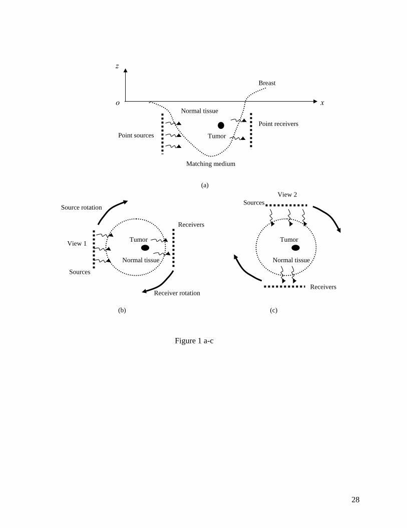
The irregular shape of the 3-D tumor is modeled using the spherical harmonics technique

similar to the work by Garboczi, in which aggregates in concrete were simulated using the

spherical harmonic functions [14]. Fig. 1 shows the configuration of the two-region breast

model assuming the patient is lying prone.

A variety of algorithms for imaging have been developed for two-dimensional (2-D) or 3-D

dielectric, conducting or perfect electric conducting objects (PEC) in both the time- and

frequency- domains [15-37]. The frequency-domain algorithms generally estimate either the

electrical properties of the object (i.e., the real and imaginary parts of the relative permittivity)

4

[16-30], or the shape and/or location of the object (assuming an a priori knowledge of its

dielectric constants) [31-32]. Most of the published frequency-domain work for shape

reconstruction is focused on 2-D PEC or dielectric objects [33-35], with few exploring 3-D shape

reconstruction of PEC objects [37], in which the object location was a priori assumed known.

The focus of the current work is to simultaneously reconstruct the shape and location of 3-D

dielectric lossy objects of arbitrary shape and location immersed in lossy medium. The basic

idea here is to implement a steepest descent gradient technique to minimize a cost functional

searching for the shape and location parameters of a tumor present in normal breast tissue. The

incident fields are calculated in the near-zone based on the model of point current source given in

[38], while the scattered fields are also computed in the near-zone using the method of moments

(MoM) upon computing the surface currents [39].

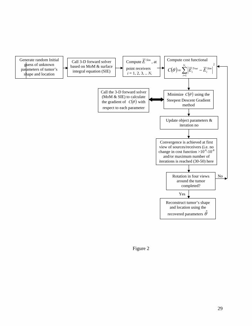
The flowchart of the presented imaging algorithm is shown in Fig. 2 and will be discussed in

Section II. In Section III, the numerical results will demonstrate the advantage of using the

multiple-view strategy that indeed improves the convergence of the imaging algorithm towards

the true tumor. We believe that this strategy helps the algorithm to avoid being trapped in local

minima similar to the advantage of using the frequency-hopping strategy [17]. The algorithm

will also be tested on corrupted synthetic data using additive white Gaussian noise [26].

As shown in Fig. 2, the algorithm requires calling the forward solver many times to

numerically calculate the gradient of the cost function with respect to each shape and location

parameter. This represents a major computational disadvantage for inverse scattering problems

especially for recovering large number of parameters. In particular, if the dielectric constant at

each pixel in the breast is to be estimated to reconstruct the image of the tumor; using this

algorithm will require excessive CPU time. The advantage here is that the tumor’s irregular

5

shape can be modeled using few parameters based on the spherical harmonic functions. The

disadvantage is the need for a priori assumption of the electrical properties of the breast and

tumor tissue. The results demonstrated the potential of the algorithm when a perfect knowledge

of the tumor’s properties is not available; however, imperfect knowledge of breast tissue

properties will lead to imperfect matching with the surrounding medium and it will cause

unwanted reflections from the breast.

II. Formulations

As mentioned earlier, we assume that the breast is surrounded by a perfectly matching

medium, the normal breast tissue is homogeneous except for the tumor tissue, and the breast skin

thickness is ignored [3], [6], [13]. In this scenario, the electromagnetic waves will scatter only

due to the presence of a tumor inside the breast. The reconstruction algorithm presented here

involves combining two techniques; the forward solver to calculate the scattered fields (i.e. the

direct method) and an optimization technique based on the steepest descent gradient method for

minimizing a cost functional (i.e. the error function) [40-42]. Due to the small size of the

scatterer (i.e. the breast tumor) in the current model, the MoM is considered a reasonable method

for the forward solver since we need only solve for the surface currents on the tumor. A brief

discussion of the incident, scattered, tumor model, and the algorithm will be given here.

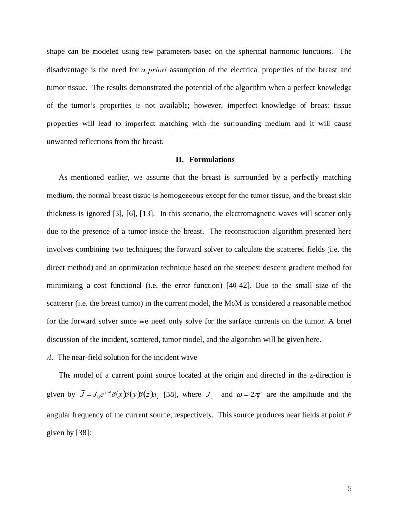
A. The near-field solution for the incident wave

The model of a current point source located at the origin and directed in the z-direction is

given by ( ) ( ) ( ) ztj azyxeJJ δδδω

0= [38], where 0J and fπω 2= are the amplitude and the

angular frequency of the current source, respectively. This source produces near fields at point P

given by [38]:

6

ϑωεε

µπ

γ

cos224 320

⎟⎟⎠

⎞⎜⎜⎝

⎛+=

−

rjreJE

r

r (1a)

ϑωεε

µωµπ

γ

ϑ sin114 320

⎟⎟⎠

⎞⎜⎜⎝

⎛++=

−

rjrrjeJE

r

(1b)

ϑγπ

γ

ϕ sin14 20 ⎟

⎠⎞

⎜⎝⎛ +=

−

rreJH

r

(1c)

where ),,( ϕϑr are the spherical coordinate system of point P and µεωγ j= is the propagation

constant of the wave. The permeability and permittivity of the medium are 0µµ = and rεεε 0= ,

respectively, where 0µ and 0ε are the permeability and permittivity of the free space. For a lossy

medium, the relative permittivity is complex given by )/( 0ωεσεε jr −′= , where σ is the

conductivity of the medium. This source also represents an infinitesimal dipole aligned in the z-

direction where the effect of changing its direction to the x- or y- directions will be investigated

in Section III.

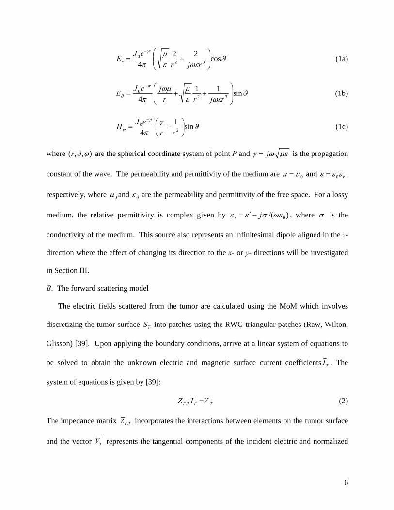
B. The forward scattering model

The electric fields scattered from the tumor are calculated using the MoM which involves

discretizing the tumor surface TS into patches using the RWG triangular patches (Raw, Wilton,

Glisson) [39]. Upon applying the boundary conditions, arrive at a linear system of equations to

be solved to obtain the unknown electric and magnetic surface current coefficients TI . The

system of equations is given by [39]:

TTTT VIZ =. (2)

The impedance matrix TTZ . incorporates the interactions between elements on the tumor surface

and the vector TV represents the tangential components of the incident electric and normalized

7

magnetic fields on the tumor surface obtained from (1). A brief summary of the formulations is

given in Appendix A.

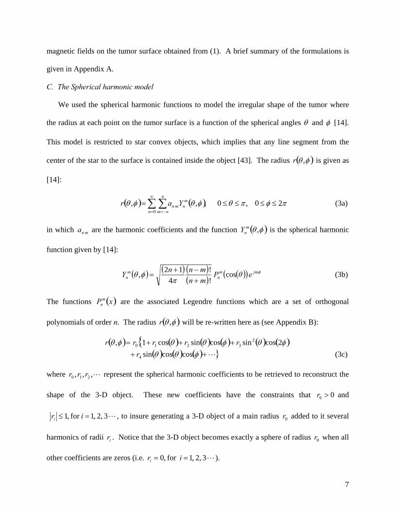
C. The Spherical harmonic model

We used the spherical harmonic functions to model the irregular shape of the tumor where

the radius at each point on the tumor surface is a function of the spherical angles θ and φ [14].

This model is restricted to star convex objects, which implies that any line segment from the

center of the star to the surface is contained inside the object [43]. The radius ( )φθ ,r is given as

[14]:

( ) ( ) (3a) 20 ,0 ,,,0

∑ ∑∞

= −=

≤≤≤≤=n

n

nm

mnmn Yar πφπθφθφθ

in which mna are the harmonic coefficients and the function ( )φθ ,mnY is the spherical harmonic

function given by [14]:

( ) ( ) ( )( ) ( )( ) (3b) cos

! !

412, φ

πφθ jmm

nm

n eθPmnmnnY

+−+

=

The functions ( )xPmn are the associated Legendre functions which are a set of orthogonal

polynomials of order n. The radius ( )φθ ,r will be re-written here as (see Appendix B):

( ) ( ) ( ) ( ) ( ) ( ){( ) ( ) ( ) } (3c) coscossin

2cossincossincos1 ,

4

23210

L+++++=

φθθφθφθθφθ

rrrrrr

where L,,, 210 rrr represent the spherical harmonic coefficients to be retrieved to reconstruct the

shape of the 3-D object. These new coefficients have the constraints that 00 >r and

L 3 ,2 ,1for ,1 =≤ ir i , to insure generating a 3-D object of a main radius 0r added to it several

harmonics of radii ir . Notice that the 3-D object becomes exactly a sphere of radius 0r when all

other coefficients are zeros (i.e. L 3 ,2 ,1for ,0 == i ri ).

8

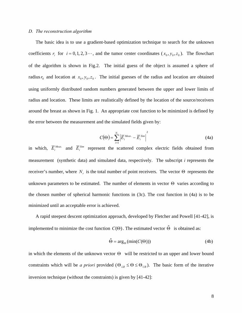
D. The reconstruction algorithm

The basic idea is to use a gradient-based optimization technique to search for the unknown

coefficients i r for L 3 ,2 ,1 ,0 =i , and the tumor center coordinates ( 000 ,, zyx ). The flowchart

of the algorithm is shown in Fig.2. The initial guess of the object is assumed a sphere of

radius 0r and location at 000 ,, zyx . The initial guesses of the radius and location are obtained

using uniformly distributed random numbers generated between the upper and lower limits of

radius and location. These limits are realistically defined by the location of the source/receivers

around the breast as shown in Fig. 1. An appropriate cost function to be minimized is defined by

the error between the measurement and the simulated fields given by:

( ) (4a) 2

1

.∑=

−=ΘrN

i

Simi

Measi EEC

in which, .MeasiE and Sim

iE represent the scattered complex electric fields obtained from

measurement (synthetic data) and simulated data, respectively. The subscript i represents the

receiver’s number, where rN is the total number of point receivers. The vector Θ represents the

unknown parameters to be estimated. The number of elements in vector Θ varies according to

the chosen number of spherical harmonic functions in (3c). The cost function in (4a) is to be

minimized until an acceptable error is achieved.

A rapid steepest descent optimization approach, developed by Fletcher and Powell [41-42], is

implemented to minimize the cost function )(ΘC . The estimated vector Θ̂ is obtained as:

(4b) )))((min(argˆ Θ=Θ Θ C

in which the elements of the unknown vector Θ will be restricted to an upper and lower bound

constraints which will be a priori provided ( UBLB Θ≤Θ≤Θ ). The basic form of the iterative

inversion technique (without the constraints) is given by [41-42]:

9

(4c) ˆˆ1 kkkk dα+Θ=Θ +

in which k is the iteration number, α is a small enough positive scalar value represents the step

at iteration k, and the vector kd is the vector that minimizes the quadratic equation ( )dq [41-42]:

( ) (4d) ,5.0 nTk

T RddcdHddq ∈+=

in which R is the real domain, ( )kCc Θ∇= ˆ is the gradient of the cost function )(ΘC , and the

matrix H contains the true curvature information for the feasible region and can be regarded as a

reduced inverse Hessian matrix [41-42]. Equations (4) show that reconstructing the 3-D tumor

requires solving the forward problem large number of times, either to compute SimiE at each

receiver in (4a) or to compute the gradient ( )kCc Θ∇= ˆ in (4d) with respect to each parameter of

vector Θ . Calculating the gradient is a key computational issue of this algorithm, which is

implemented here using the forward finite difference approximations [44]. The shape of the 3-D

tumor becomes more irregular upon increasing the number of spherical harmonics in (3c),

leading to increase in the required CPU time as will be demonstrated in Section III.

III. Numerical Results

In this section, we demonstrate the efficiency of the algorithm using several numerical

examples. Several point sources and receivers are located around the breast as shown in Fig. 1.

In all examples presented here, the sources and receivers are transmitting or receiving waves

from four views around the breast described as (with 200 0 −≥≥ z cm):

(1) View1: cm50 −=x and cm25cm5 0 ≤≤− y , (2) View2: cm250 =y and cm25cm5 0 ≤≤− x ,

(3) View3: cm250 =x , cm25cm5 0 ≤≤− y , (4) View4: cm50 −=y and cm25cm5 0 ≤≤− x

In all results presented here, the source frequency is assumed 6 GHz. Based on several

numerical examples, it is observed that a maximum number of iterations ranging from 30 to 50

10

per view is reasonable. In this work, the upper and lower constraints on the object location are:

cm15cm5 0 ≤≤ x , cm15cm5 0 ≤≤ y , cm15cm5 0 −≤≤− z , while the constraints on the object’s

radii are: 0.25cm ≤ r0 ≤ 5cm, 0≤ ri ≤ 0.45, i = 1, 2, 3... (noting that ri has no units, see eq. 3c).

The amplitude of the point current source in (1) is 0J = 1 mA and is aligned in the z-direction

unless otherwise is stated [38]. All computations are conducted using the HP DS25 (COMPAQ

ALPHA) EV68/1000MHz server. The examples considered here are summarized in Table 1.

Table 1 Summary of numerical examples

(i) Algorithm Strategy

The flowchart of the algorithm is shown in Fig. 2 and it proceeds as follows; (i) the initial

guesses of tumor radius and position are generated randomly with assuming the tumor as a

sphere by setting all harmonic coefficients to zero, (ii) the point sources and receivers are

arranged according to View1 shown in Fig. 1b, (iii) the algorithm is executed for certain number

of iterations (30-50 iterations per view in this work), (iv) the cost function is updated at each

iteration, (v) T/R pairs are rotated to View 2 as shown in Fig. 1c is utilized with updating the

initial guess from the results obtained in View 1. This mechanism is repeated using View 3 and

View4. This reconstruction algorithm represents a “marching on in view” technique.

The true tumor is generated in all cases using 360 RWG patches and 182 surface nodes;

however, the reconstruction algorithm is set to use only 270 RWG patches and 137 nodes in

generating the reconstructed tumor in each inversion iteration. This implies that using different

Figure Purpose Figure Purpose Fig. 3 Marching vs simultaneous views Fig. 8 Imperfect knowledge of tumor’s rε̂ Fig. 4 Seven parameters with r0 = 2cm Fig. 9 Source polarization effect Fig. 5 Seven parameters with r0 = 1cm Fig. 10 Data corrupted with Gaussian noise Fig. 6 Seven parameters with r0 = 5mm Fig. 11 Data contains unknown clutter Fig. 7 Thirteen parameters with r0 = 1.75cm

11

MoM discretization and different numbers of the spherical harmonics render the synthetic data to

be non-ideal and more realistic.

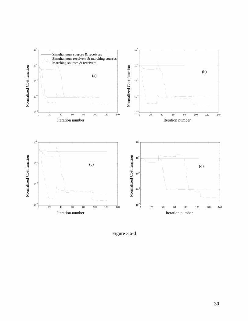
(ii) Marching on in views vs simultaneous views

The use of a gradient descent approach brings with it a host of difficulties in terms of local

minima. Global methods which avoid these problems (in theory) are well studied but still rather

intensive. Reports in the literature indicate that various methods of cycling through the data can

help avoid local minima while still allowing us to employ the relatively straightforward gradient

descent optimization method. Here we seek to understand through experiments the merits of

these choices in the context of the breast imaging problem at hand.

In this example, we examine three options of inverting data collected using point

transmitters/receivers (T/R) located around the target. For simplicity, a sphere of radius 2.5 cm

and relative dielectric constant 1250 jr −=ε immersed in air will be used as the target. The true

sphere is located at cm5.70 =x , 35.60 =y cm, and cm100 −=z . The resolution of the point T/R

locations is ~ 0.468 cm in the x- or y- directions and ~ 0.625 cm in the z-direction as described

earlier. These three options are summarized as:

(1) Option 1 is to simultaneously invert using data collected from all T/R pairs, i.e. using

4×1088 = 4352 pairs located at all four views (solid line in Fig. 3).

(2) Option 2 is to invert data collected using 1088 sources located at View1 and receiving

simultaneously at all 4×1088 = 4352 receiver located at all four views. Then use the

rotated 1088 sources at View2 and simultaneously receive at all 4352 receiver located at

all four views, etc. The parameters estimated using the sources at View1 are used as

initial guess for the rotated sources at View2, etc (dashed-line in Fig. 3).

12

(3) Option 3 is to invert data collected using only 1088 T/R pairs at a time, where the sources

are located at View1 and the receivers are located at the opposite side (View3). This

means that 1088 T/R pairs are used for 30 iterations and then rotated simultaneously as

shown in Fig. 1, etc. (dot-dashed-line in Fig. 3).

In Figs. 3a-d, four randomly generated initial guess of the sphere radius and location

( 0000 ,,, zyxr ) are presented as: 5.11 ,9 ,865.6 ,225.1 − cm in Fig. 3a, 5.6 ,6.34 ,12.3 ,443.0 − cm in

Fig. 3b, 7 ,1.9 ,8.05 ,57.3 − cm in Fig.3c, and 4.14 ,8.4 ,11.3 ,77.0 − cm in Fig. 3d.

The results of Fig. 3 show the potential of the algorithm to invert data based on options 2 and

3. Sometimes a temporary increase in the error function is observed upon changing the view;

however ultimately it reduces and convergence is achieved. The reconstructed spheres show

very good agreement with the true one (not presented here). It seems that this strategy helps the

algorithm to avoid being trapped in local minima similar to the advantage of using the

frequency-hopping strategy [17]. Based on these results, we have adopted the strategy of

marching on in view (Option 3) in the remainder of this work.

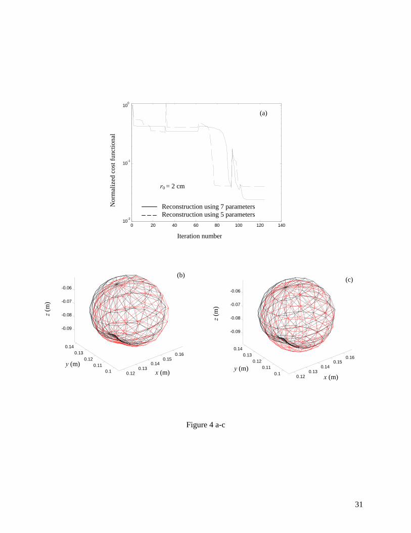
(iii) Reconstruction of arbitrary shape and location

In all remainder examples, the two-region model of the breast with an immersed tumor will

be used. In Example 2, the true tumor is generated using seven unknown coefficients including

four spherical harmonics and three unknowns for the center location ( 000 ,, zyx ). At 6 GHz, the

healthy and malignant breast tissues are assumed to have relative dielectric constants of

2.19 jr −=ε and 1250 j− , respectively, [5]. At this frequency, the wavelength in breast tissue

is approximately 1.6 cm. The true tumor is non-spherical as shown in Fig. 4 with true

parameters as r0 = 2cm, r1 = 0.678, r2 = 0.495, r3 = 0.11 (see eq. 3c) and true location at x0 =

13.35cm, y0 = 11.95cm, z0 = -8.5cm. Several initial guesses are successfully examined; however,

13

the specific initial guesses in Fig. 4 are r0 = 3.57cm, x0 = 8.05cm, y0 = 9.1cm, z0 = -7cm with all

higher order harmonic coefficients initially set to zeros (r1 =r2 =r3 = 0). The reconstructed tumor

is obtained using seven unknowns in Fig. 4b and five unknowns in Fig. 4c. The true tumor is

shown in black and the reconstructed tumor is shown in red. The normalized cost function is

plotted in Fig. 4a for both cases showing the reduction in the error upon increasing the inversion

iterations. The results show good agreement between the reconstructed and true tumor in both

cases. The CPU time required for reconstructing the tumor in Fig. 4b and 4c is ~12-13 hrs.

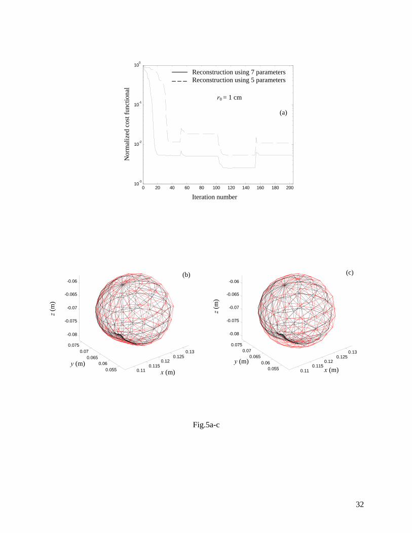
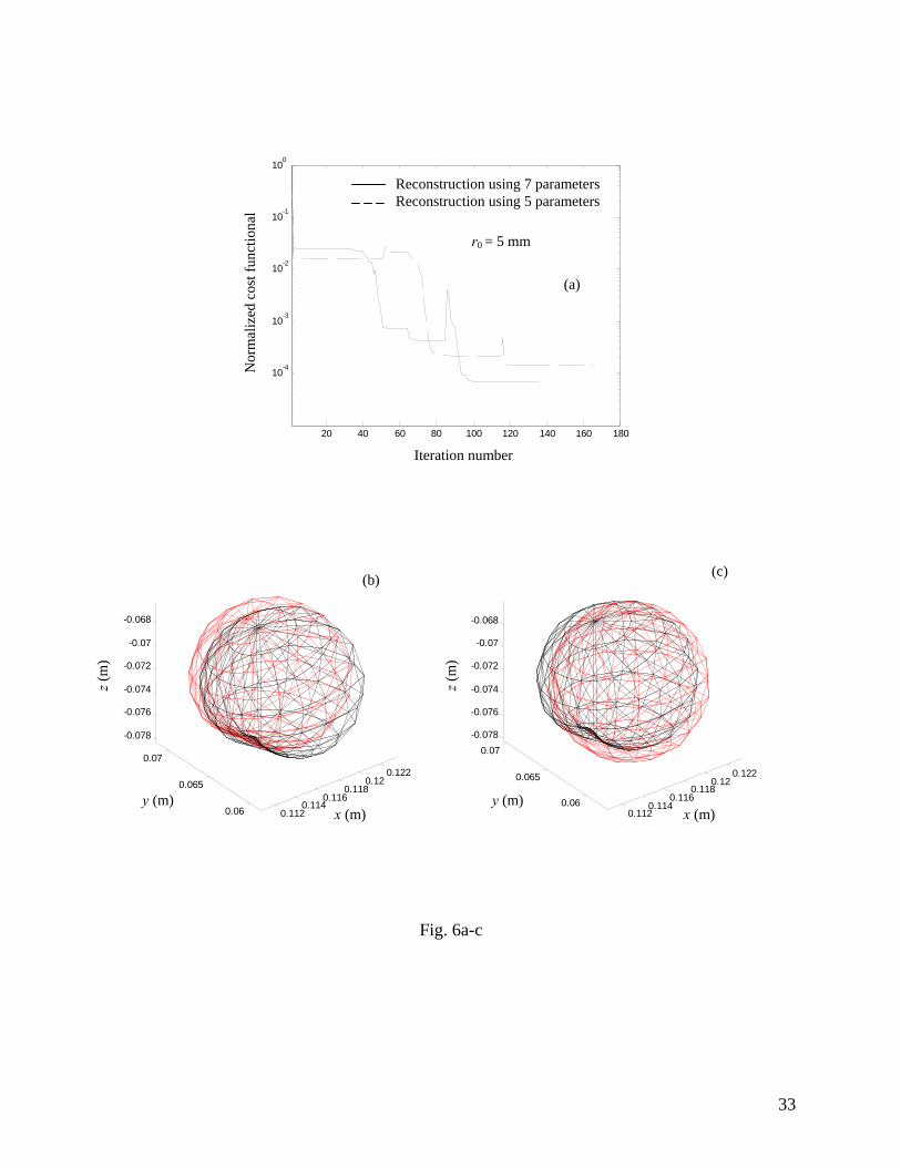
To show the capability of the algorithm in reconstructing smaller tumors, the same data of

Fig. 4 are used in Figs. 5 and 6 but for tumors with r0 = 1cm in Fig. 5 and r0 = 5mm in Fig. 6.

As shown in the flow chart of Fig. 2, the convergence of the algorithm could be achieved if the

change in the cost function is less than a tolerance of 10-6-10-8 or if the maximum number of

iterations is reached (50 in this example). The results of Figs. 5 and 6 show the potential of the

algorithm in reconstructing smaller tumors.

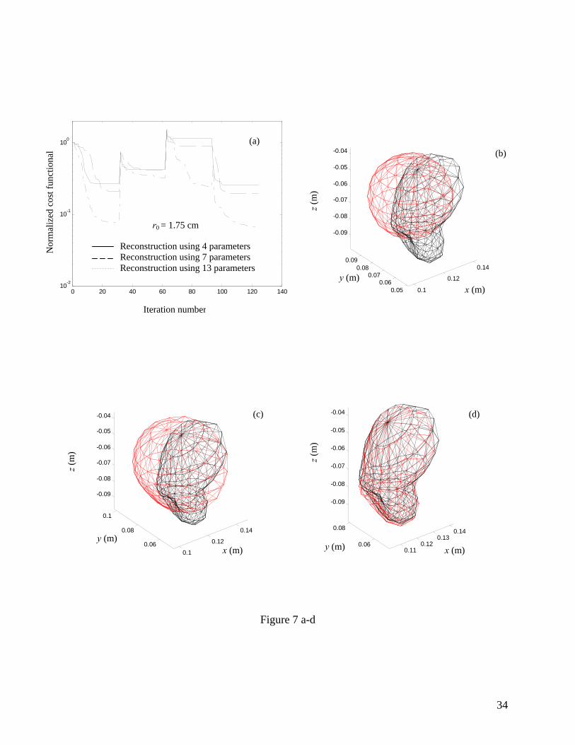
Example 3 will demonstrate the reconstruction of a tumor of more irregular shape as shown

in Fig. 7. The true tumor is generated using thirteen parameters with true values as: r0 = 1.75cm,

r1 = 0.365, r2 = 0.266, r3 = 0.059, r4 = 0.217, r5 = 0.282, r6 = 0.162, r7 = 0.322, r8 = 0.265, r9 =

0.025 (see eq. 3c) and location at x0 = 11.5cm, y0 = 6.45cm, z0 = -7.5cm. The reconstruction is

based on using four parameters in Fig. 7b (i.e. a sphere), seven parameters in Fig. 7c, and

thirteen parameters in Fig. 7d.

Notice that the cost function associated with the thirteen-parameter reconstruction is smaller

than that of the four or the seven-parameter reconstructions. Also, as expected using the thirteen

parameters in the reconstruction potentially provides more accurate reconstruction of the tumor

shape. It is interesting to observe that in this example when the reconstruction has been initially

14

attempted for the thirteen parameters; no convergence was achieved. However, when the

reconstruction was conducted using four parameters (i.e. a sphere) and then using the estimated

values of 0000 ,,, zyxr as initial guess for the thirteen unknown reconstruction; a good agreement

with the true tumor is obtained as shown in Fig. 7d. It is observed that initially using only four

unknowns in the reconstruction leads to accurate estimation of the location 000 ,, zyx , while re-

iterating the algorithm using more parameters leads to more accurate reconstruction of the shape

upon comparing Fig. 7d with 7b. This conclusion is consistent with the work by Tortel and

Saillard in [37]. The total CPU time for Fig. 7b is ~24 hrs, for Fig. 7c is ~ 21 hrs, and for Fig. 7d

is ~22 hrs (without including the CPU time required for Fig. 7b).

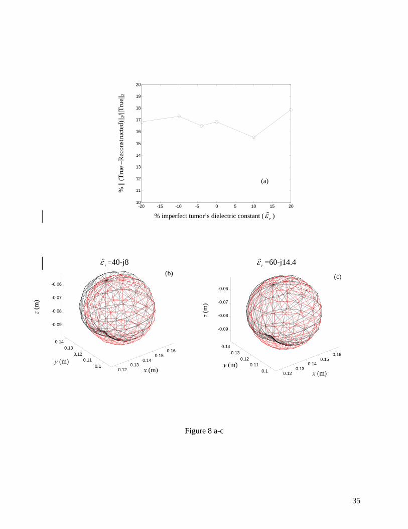
(iv) Imperfect knowledge of tumor’s electrical properties

In all examples presented earlier, the complex dielectric constant of the tumor is a priori

assumed known. The effect of imperfect knowledge of the tumor’s electrical properties is

examined in Example 4. The true value of the tumor’s complex dielectric constant at 6 GHz, as

used to generate all synthetic data, is rε = 50-j12 [5]. The true tumor generated using seven

unknowns and reconstructed using five unknowns of Example 2 (Fig. 4) is used here. The

relative error in the estimated parameters is expressed as 22

/ˆ TrueTrue ΘΘ−Θ , where 2

.

represents the norm-2, Θ̂ represents the estimated vector parameters of the reconstructed tumor

and TrueΘ represents the true vector parameters. This error is plotted in Fig. 8a vs the error in the

tumor’s complex dielectric constant rε̂ . In this example, TrueΘ has a length of seven while Θ̂

has a length of five (see Fig. 4), therefore zero padding is used to make the two vectors of equal

lengths (i.e. r2 and r3 are assumed zeros in Θ̂ ). The zero value in the axis of rε̂ in Fig. 8a

represents the perfect knowledge of the true dielectric constant (similar to Fig. 4), while the

15

positive or the negative values of rε̂ implies imperfect knowledge with larger or smaller values

of the true rε , respectively. Notice that a relative error in the reconstruction ~ 17% (in the

vertical-axis) is associated with the zero error in rε . This can be explained by the fact that the

reconstruction is based on using only five parameters instead of seven parameters which causes

an error of only 7%. The results of Figs. 8b-c show that the algorithm has a potential of

providing good reconstruction of the tumor with uncertainty in its dielectric constant up to ±20%

which implies that rε̂ = 40-j8 for the -20% error and rε̂ = 60-j14.4 for the +20% error. This can

be explained by the fact that even with ±20% error in rε̂ , still there is a large contrast between

the electrical properties of the tumor and the surrounding medium ( rε =9-j1.2) [5].

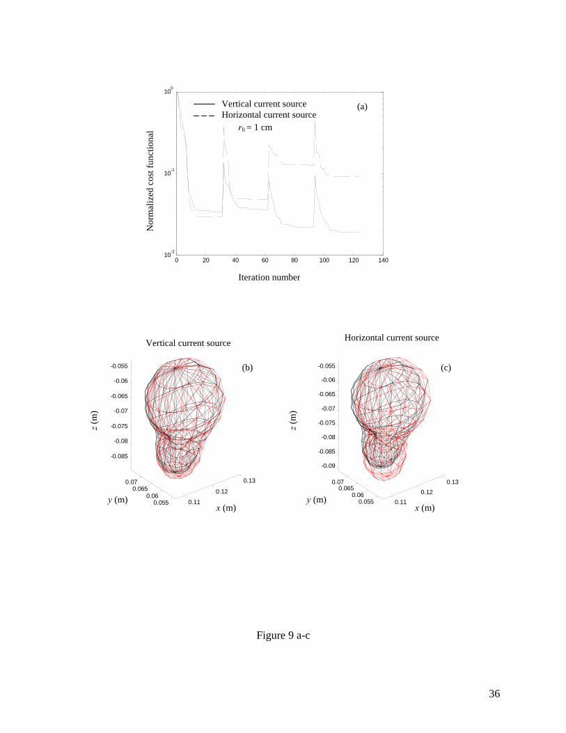
(v) Effect of source polarization

In all results presented in this section, the current source is assumed in the z-direction as

given in (1) which is in the vertical-direction (see Fig. 1). When the current source is oriented

horizontally, it will be in the y-direction at View1 and View 3, and in the x-direction at View 2

and View 4 (see Fig. 1). Example 5 shows the reconstruction of a new tumor that has a

dimension in the z-direction larger than the dimensions in the x-y cross section as shown in Fig.

9. The true tumor is generated using ten parameters with true values as: r0 = 1 cm, r1 = 0.475, r2

= 0.347, r3 = 0.077, r4 = 0.282, r5 = 0.282, r6 = 0.211 (see eq. 3c) and location at x0 = 11.5cm, y0

= 6.45cm, z0 = -7.5cm. In this particular example, when all ten parameters of the original tumor

are attempted to be recovered using random initial guesses, a convergence to the true parameters

has been achieved only when vertical current sources are used. No advantage is observed when

data of both vertical and horizontal current sources are used simultaneously. On the other hand,

when starting the reconstruction assuming the tumor is a sphere and then using the recovered

four parameters as initial guess to re-reconstruct the irregular tumor, both source polarizations

16

provide good image reconstruction as shown in Figs. 9b and 9c, respectively. This observation is

consistent with the results of Fig. 7 and with the work by Tortel and Saillard in [37]. Notice that

Fig. 9a shows a monotonic decrease in the cost function when vertical sources are used, except

for View 2 where a slight increase is observed, which is not the case for the horizontal case. The

later case shows a cost function error of 2.5% at View1 compared with 7.9% at View4, leading

to insignificant improvement when the image is reconstructed using the parameters recovered at

View1 instead of View4 (not presented here). Notice that all images presented in this work are

reconstructed using the parameters recovered after four views. The results of Figs. 9b and 9c

show a slight improvement in the image when using vertical sources.

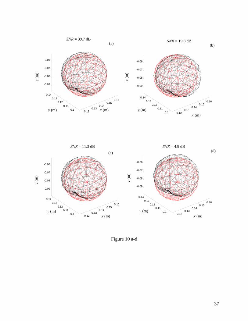
(vi) Random noise added to synthetic data

In Example 6, the synthetic data obtained at 6 GHz, are corrupted by adding random

Gaussian white noise. Several definitions are considered in the literature concerning adding

random noise to synthetic data; however, we adopted the definition used in [26] where the

signal-to-noise-ratio (SNR) is: dB (log 10 22

10 )n/nESNR True += , where TrueE denotes the

vector of the noiseless synthetic data and n represents a complex noise vector of length NvNr,

where Nv is the number of views (four in this work) and Nr is the number of receivers at each

view (1088 point receivers here). The real and imaginary parts of the vector n are generated by

two independent sequences of white Gaussian variables characterized by zero mean and standard

deviation σn. In the current work, several values of σn ranging from 0.001 to 0.3 are examined

which gives SNR ranges from 39 to 5dB. The true tumor used in Example 2 (or Fig. 4) is also

used here to investigate the effect of adding Gaussian noise on the reconstruction accuracy. The

images in Fig. 10 a-d show the potential of the algorithm to reconstruct a tumor with data SNR =

39.7 dB, 19.8 dB, 11.3 dB and 4.9 dB, respectively.

17

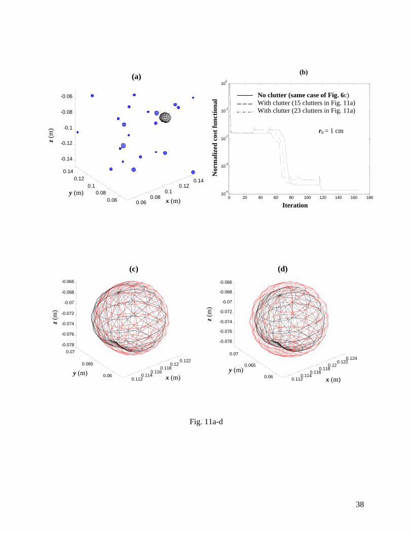
(vii) Data contains unknown clutter

In Example 7, the background contains discrete clutters that randomly vary in size and

medium. A total of twenty three small spheres are randomly generated with different radii,

locations and media as shown in Fig. 11a. For simplicity, all interactions between these small

scatterers and with the tumor are ignored. The data in this example are the same as in Fig. 6c

with tumor’s main radius r0 = 5mm, rε = 9 – j1.2 for the background and rε = 50 - j12 for the

tumor.

The relative dielectric constant of the first fifteen small spheres randomly ranges from 6 to 15

for the real part and from 0.5 to 1.5 for the imaginary part. To increase the level of clutter, an

additional eight small spheres are added to the background with the real and imaginary parts

randomly range from 5 to 40 and from 1.5 to 11, respectively. The maximum radius among all

small spheres is almost 5.22% of the tumor’s main radius r0 and it occurs in the first set, while it

is almost 3.73% in the additional set of eight spheres.

The data of the scattered electric fields due to the tumor and the clutter are inverted assuming

that the clutter is unknown. The normalized cost functional is plotted in Fig. 11b for three cases;

without clutter (same as Fig. 6c) and with clutter of fifteen and twenty three small spheres are

present in the background. The reconstruction results for the clutter cases are plotted in Figs. 11c

and 11d, respectively. The results in Fig. 11c show a reasonable accuracy of the algorithm even

with clutter in the background, while the results in Fig. 11d show the deterioration in the

accuracy as the clutter level increases.

Although all the results presented in this section are based on using 6 GHz; however, the

algorithm has been successfully tested upon combining information from several frequencies

18

ranging from 3 GHz to 8 GHz using plane wave source (not presented here). The results were

consistent with those obtained using the frequency hopping strategy [17].

IV. Conclusions

In this work, an optimization algorithm to simultaneously reconstruct the shape and location

of breast cancer tumors is developed and tested. The results suggest collecting data using

multiple views in the experiment to achieve the best possible reconstruction of the tumor. The

algorithm shows a potential of good reconstruction of the tumor even when the synthetic data is

corrupted with random Gaussian noise. In addition, increasing the number of spherical

harmonics in the model leads to better capturing of the tumor shape but it takes more CPU time.

Other challenges need to be investigated such as the breast interior inhomogeneities, due to

the fat and glandular tissue, and the imperfect knowledge of normal breast tissue properties.

Addressing these issues will help toward the use of this technique to breast tumor imaging,

which will be the focus of separate work. Another issue is that too much time is required to

produce the images. This factor depends on the number of spherical harmonics utilized to

reconstruct the tumor as well as the level of noise in the data. Parallel programming is one

possible way to speed up the algorithm.

Appendix A

The Poggio, Miller, Chang, Harrington and Wu (the PMCHW) equations are used for

dielectric scatterers [39]. The electric and magnetic surface currents ( TJ , TM ) are related to the

unknown vector coefficient TI through the conventional MoM approximation given by [39]:

( ) ( ) ( ) ( ) (A1) ,1

201

1 Tn

N

nnTn

N

nnT Sr, rjIηrM rjIrJ ∈== ∑∑

==

19

in which j is the vector basis function and [ ]21 IIIT = represents the electric and magnetic

current coefficient vector, with total number of current coefficients unknown equal to N2 . The

normalization factor 0η is the intrinsic impedance of the free space. The impedance matrix TTZ .

is given by [39]:

( ) ( )

( ) (A2) ,,

,,

22

221

120210

21021

.

⎟⎟⎟⎟

⎠

⎞

⎜⎜⎜⎜

⎝

⎛

⎟⎟⎠

⎞⎜⎜⎝

⎛++

+−+

=

T

T

TT

SS

SS

TT jLLjjKKj

jKKjjLLj

Zηη

ηη

η

The operators 1L , 2L , 1K , and 2K are derived in [39] and given by:

( ) ( ) (A3) 2,12,1

2,12,12,1 sdrXirXiXLTS

′⎪⎭

⎪⎬⎫

⎪⎩

⎪⎨⎧

Φ′⋅∇′∇+′Φ= ∫ ωεωµ

( ) (A4) 2,12,1 sdrXXKTS

′Φ∇×′= ∫

in which the 3-D scalar Green’s function for region l is lΦ = ( ) rrrrikl ′−′−− π4/exp with the

associated wave number lllk µεω= . The intrinsic impedances of the two regions are 1η and

2η (i.e. the surrounding medium and the tumor), respectively. The complex inner product

between two vector functions A and B is expressed by ∫ ⋅=S

SdsBABA *, .

Appendix B

Upon truncating the infinite summation in (3a) as:

( ) ( ) (B1) 20 ,0 ,,,0

∑ ∑= −=

≤≤≤≤≈N

n

n

nm

mnmn Yar πφπθφθφθ

For simplicity, let N = 4

( ) ( ) ( ) ( ) (B2) ,,,,1

1

4

44411

0000 ∑ ∑

−= −=

+++≈m m

mm

mm YaYaYar φθφθφθφθ K

20

Upon substituting (3b) in (B2), we obtain

( )( )( )( )

( )φφ

φφ

φφ

φφ

π

π

π

π

πφθ

4)4(4

4)4(4

44

)1(2)1(212

2)2(2

2)2(2

22

)1(1)1(11

1

0000

)!84/(9

)!34/(5

)!44/(5

)!24/(3

4/1,

jj

jj

jj

jj

eaeaP

eaeaP

eaeaP

eaeaP

Par

+×+

+

++−×+

++×+

+−×+

≈

−−

−−

−−

−−

K

(B3)

For the radius ( )φθ ,r to be real number, we use )()( )1( mnm

mn aa −=− in (B3). After some

algebraic manipulations noting that mnP is a function of θ [14], we obtain:

( ) ( ) ( ) ( ) ( ) ( ){ ( ) ( ) ( )( ) ( ) ( ) ( ) ( )

( ) ( ) ( ) ( )} (B4) cos coscossin

2coscossin3cossin)(cos

coscossin2cossincossincos1 ,

414

313

27

36

25

42

3210

θφθθ

φθθφθθ

φθθφθφθθφθ

rr

rrr

rrrrrr

++

++++

++++≈

K

Notice that choosing N = 4 in (B1) provides up to fifteen ri’s coefficients in (B4).

ACKNOWLEDGMENTS

This research was sponsored in part by the Arkansas Biosciences Institute award no. ABI-21-

0103, the Women Giving Circle at the University of Arkansas grant no. WGC-22-0000, the

National Science Foundation award no. ECS-0524042, and the NSF-ERC (CenSSIS) at

Northeastern University award no. EEC-9986821.

21

References

[1] P. M. Meaney, M. W. Fanning, D. Li, S. P. Poplack and K. D. Paulsen, “A clinical

prototype for active microwave imaging of the breast,” IEEE Trans. Microwave Theory

Tech., vol. 11, pp. 1841-1853, 2000.

[2] P. M. Meaney, K.D. Paulsen and J. T. Chang, “Near-field microwave imaging of

biologically-based materials using a monopole transceiver system,” IEEE Trans.

Microwave Theory Tech., vol. 46. pp. 31-45, 1998.

[3] X. Li and S. C. Hagness, “A confocal microwave imaging algorithm for breast cancer

detection,” IEEE Microwave and Wireless Components Letters, vol. 11, pp. 130-132,

March 2001.

[4] E. C. Fear and M. A. Stuchly, “Microwave detection of breast cancer,” IEEE Trans.

Microwave Theory and Tech., vol. 46, pp. 1854-1863, November 2000.

[5] S. Hagness, A. Taflove and J. E. Bridges, “Three-dimensional FDTD analysis of a pulsed

microwave confocal systems for breast cancer detection: Design of an antenna-array

element,” IEEE Trans. Antennas Propagat., vol. 47, pp. 783-791, May 1999

[6] E. J. Bond, X. Li, S. Hagness and B. D. Van Veen, “Microwave imaging via space-time

beamforming for early detection of breast cancer,” IEEE International Conference on

Acoustics, Speech, and Signal Processing, vol. 3, pp. 2909–2912, May 13-17, 2002.

[7] E. C. Fear, S. C. Hagness, P. M. Meaney, M. Okoniewski, and M. Stuchly, “Enhancing

breast tumor detection with near-field imaging,” IEEE Microwave magazine, pp.48-56,

March 2002.

22

[8] Q. Fang, P. M. Meaney, S. D. Geimer, A. V. Streltsov and K. D. Paulsen, ”Microwave

image reconstruction from 3-D fields coupled to 2-D parameter estimation,” IEEE Trans.

Med. Imag., pp. 475-484, vol. 23, no. 4, April 2004.

[9] A. M. Campbell and D. V. Land, “Dielectric properties of female human breast tissue

measures in vitro at 3.2 GHz,” Phys. Med. Biol., vol. 37, no. 1, pp. 193-210, 1992.

[10] Bruce Alberts, Dennis Bray, Julian Lewis, Martin raff, Keith Roberts and James D.

Watson, Molecular Biology of the Cell, Garland Publishing, Inc. New York & London,

second edition, 1989.

[11] Gregory Boverman, Ang Li, Quan Zhang, Tina Chaves, Eric L. Miller, Dana H Brooks,

and David A Boas, “Quantitative Spectroscopic Diffuse Optical Tomography Guided by

Imperfect A Priori Structural Information,” submitted to Physics in Medicine and

Biology, April 2005.

[12] J. Lin and W. C. Chew, “Solution of the three-dimensional electromagnetic inverse

problem by the local shape function and the conjugate gradient fast Fourier transform

methods,” J. Opt. Soc. Am. A, vol. 14, no. 11, pp. 3037-3045, November 1997.

[13] Q. H. Liu, Z. Q. Zhang, T. T. Wang. J. A. Bryan, G. A. Ybarra, L. W. Nolte and W. T.

Joines, “Active microwave imaging I−2-D forward and inverse scattering methods,”

IEEE Trans. Microwave Theory and Techniques, vol. 50, no. 1, pp. 123-133, January

2002.

[14] E. J. Garboczi, “Three-dimensional mathematical analysis of particle shape using X-ray

tomography and spherical harmonics: application to aggregates used in concrete,”

Cement and Concrete Research, vol. 32, no. 10, pp. 1621-1638, October 2002.

23

[15] W. C. Chew, Advances in Computational Electrodynamics, chapter 12: Imaging and

inverse problems in electromagnetics, Ed. A. Taflove, Artech House, Boston, pp. 653-

702, 1998.

[16] W. C. Chew and Y. M. Wang, “Reconstruction of two-dimensional permittivity

distribution using the distorted Born iterative method,” IEEE Trans. Med. Imag., vol. 9,

no. 2, pp. 218-225, December 1991.

[17] W. C. Chew and J. H. Lin, “A frequency-hopping approach for microwave imaging of

large inhomogeneous bodies,” IEEE Microwave and Guided Wave Letters, vol. 5, no. 12,

pp. 439-441, December 1995.

[18] K. D. Paulsen, P. M. Meaney, M. J. Moskowitz and J. H. Sullivan, Jr., “A dual mesh

scheme for finite element based reconstruction algorithms,” IEEE Trans. Med. Imag.,

vol. 14, no. 3, pp. 504-514, September 1995.

[19] P. M. Meaney, K. D. Paulsen, B. W. Pogue and M. I. Miga, “Microwave image

reconstruction utilizing log-magnitude and unwrapped phase to improve high-contrast

object recovery,” IEEE Trans. Med. Imag., vol. 20, no. 2, pp. 104-116, Feb. 2001.

[20] N. Joachimowicz, C. Pichot and J. Hugonin, “Inverse scattering: an iterative numerical

method for electromagnetic imaging,” IEEE Trans. Antenn. Propag., vol. 39, no. 12,

December 1991.

[21] N. Joachimowicz, J. J. Mallorqui, J. Bolomey and A. Broquetas, “Convergence and

stability assessment of Newton-Kantorovich reconstruction algorithms for microwave

tomography,” IEEE Trans. Med. Imag., vol. 17, no. 4, pp.562-570, August 1998.

24

[22] A. Abubakar, R. M. van Berg and J. J. Mallorqui, “Imaging of biological data using

multiplicative regularized contrast source inversion method,” IEEE Trans. Microwave

Theory and Techniques, vol. 50, no. 7, pp. 1761-1771, July 2002.

[23] A. Abubakar, P. M. van Berg and S. Y. Semenov, “A robust iterative method for Born

inversion,” IEEE Trans. Geosci. Remote Sen., pp. 342-354, vol. 42, no. 2, Feb. 2004.

[24] J. T. Rekanos, T. V. Yioultsis and T. D. Tsiboukis, “Inverse scattering using the finite-

element method and a nonlinear optimization technique,” IEEE Trans. Microwave

Theory and Techniques, vol. 47, no. 3, pp. 336-344, March 1999.

[25] K. I. Schultz and D. L. Jaggard, “Microwave projection imaging for refractive objects: a

new method,” J. Opt. Soc. Am. A, vol. 4, no. 9, pp. 1773-1782, September 1987.

[26] S. Caorsi, G. L. Gragnani, M. Pastorino, “Reconstruction of dielectric permittivity

distributions in arbitrary 2-D inhomogeneous biological bodies by a multiview

microwave numerical method,” IEEE Trans. Med. Imag., vol. 12, no. 2, pp. 232-239,

June 1993.

[27] C. Chiu and R. Yang, “Electromagnetic imaging for complex cylindrical objects,” IEEE

Trans. Med. Imag., vol. 14, no. 4, pp. 752-756, December 1995.

[28] A. E. Bulyshev, s. y. Semenov, A. E. Souvorov, R. H. Svenson, A. G. Nazarov, Y. E.

Sizov, and G. P. Tatsis “Computational modeling of three-dimensional microwave

tomography of breast cancer,” IEEE Trans. Biomed. Eng., vol. 48, no. 9, pp. 1053-1056,

2001.

[29] A. Abubakar, P.M. van den Berg and S. Y. Semenov, “Two- and three-dimensional

algorithms for microwave imaging and inverse scattering,” Progress In Electromagnetic

Research, vol. 37, pp. 57-79, 2002.

25

[30] Z. Q. Zhang, and Q. H. Liu, “3-D nonlinear image reconstruction for microwave

biomedical imaging,” IEEE Trans. Biomed. Eng., vol. 51, no. 3, pp. 544-548, 2004.

[31] K. Belkebir, E. E. Kleinman and C. Pichot, “Microwave imaging−Location and shape

reconstruction from multifrequecny scattering data,” IEEE Trans. Microwave Theory &

Techniques, vol. 45, 4, pp. 469-476, April 1997.

[32] E. L. Miller, M. Kilmer and C. Rappaport, “A new shape-based method for object

localization and characterization from scattered field data,” IEEE Trans. Geosci. Remote

Sens., vol. 38, pp. 1682-1696, 2000.

[33] C. C. Chiu and Y. Kiang, “Microwave imaging of multiple conducting cylinders,” IEEE

Trans. Antenn. Propag., vol. 40, no. 8, pp. 933-941, August 1992.

[34] C. Chiu and Y. Kiang, “Electromagnetic inverse scattering of a conducting cylinder

buried in a lossy half-space,” IEEE Trans. Antenn. Propag., vol. 40, no. 12, Dec. 1992.

[35] A. Qing, “Electromagnetic imaging of two-dimensional perfectly conducting cylinders

with transverse electric scattered field,” IEEE Trans. Antenn. Propag., vol. 50, no. 12, pp.

17861-1794, vol. 50, no. 12, December 2002.

[36] I. T. Rekanos and T. D. Tsiboukis, “An inverse scattering technique for microwave

imaging of binary objects,” IEEE Trans. Microwave Theory and Techniques, vol. 50, no.

5, May 2002.

[37] Herveʹ Tortel and Marc Saillard, “Shape reconstruction of 3D perfectly conducting

object,” proceeding of the URSI-GA, paper no 0899, July-August 2002

[38] Donald W. Dearholt and William R. McSpadden, Electromagnetic Wave Propagation,

McGraw-Hill Book Company, 1973.

26

[39] L. Medgyesi-Mitschang, J. Putnam and M. Gedera, “Generalized method of moments for

three–dimensional penetrable scatterers,” J. Opt. Soc. Am. A, vol. 11, no. 4, pp. 1383-

1398, April 1994.

[40] M. El-Shenawee and E. Miller, “Multiple-incidence/multi-frequency for profile

reconstruction of random rough surfaces using the three-dimensional electromagnetic fast

multipole model,” IEEE Trans. Geosci. & Remote Sens., vol. 42, no. 11, pp. 2499-2510,

November 2004.

[41] R. Fletcher, “A new approach to variable metric algorithms,” The Computer Journal, vol.

13, no. 3, pp. 317-322, August 1970.

[42] R. Fletcher, Practical Methods of Optimization, volume 2, John Wiley & Son, 1981.

[43] Eric W. Weisstein et al. “Star Convex.” From MathWorld--A Wolfram Web Resource.

http://mathworld.wolfram.com/StarConvex.html

[44] Matthew N. O. Sadiku, Numerical Techniques in Electromagnetics, 2nd. Ed., CRC Press

LLC, Boca Raton, FL, 2001.

27

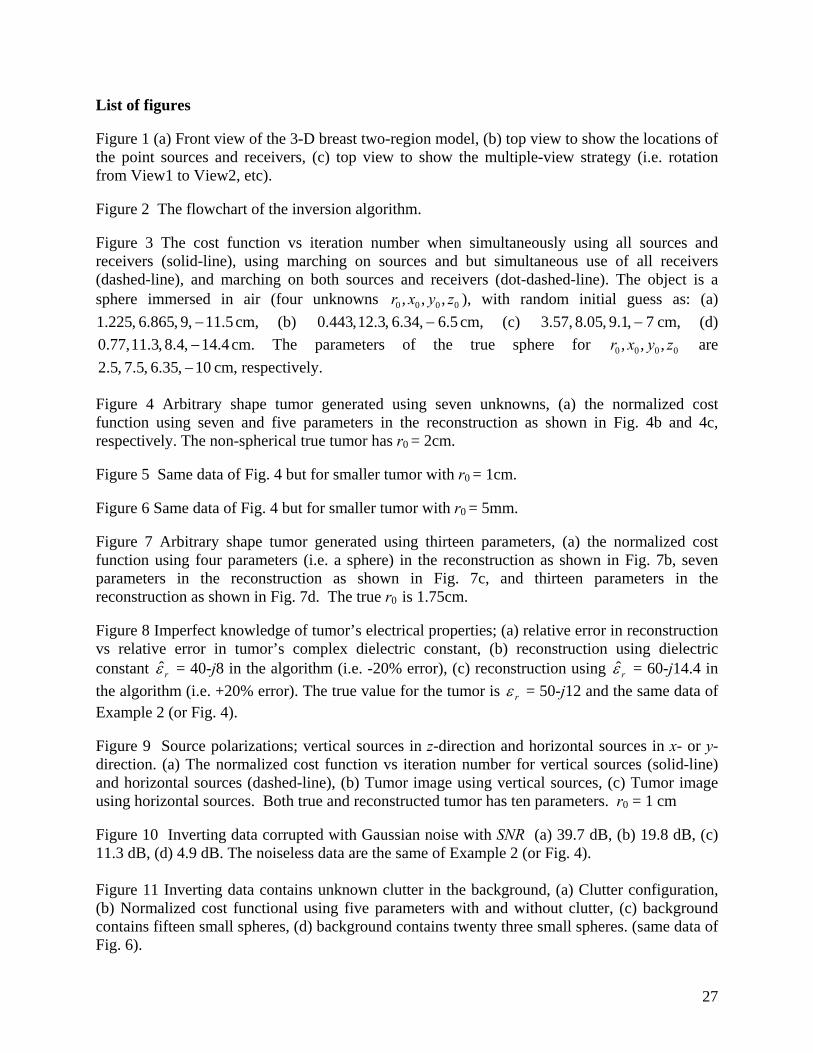
List of figures Figure 1 (a) Front view of the 3-D breast two-region model, (b) top view to show the locations of the point sources and receivers, (c) top view to show the multiple-view strategy (i.e. rotation from View1 to View2, etc). Figure 2 The flowchart of the inversion algorithm. Figure 3 The cost function vs iteration number when simultaneously using all sources and receivers (solid-line), using marching on sources and but simultaneous use of all receivers (dashed-line), and marching on both sources and receivers (dot-dashed-line). The object is a sphere immersed in air (four unknowns 0000 ,,, zyxr ), with random initial guess as: (a)

5.11 ,9 ,865.6 ,225.1 − cm, (b) 5.6 ,6.34 ,12.3 ,443.0 − cm, (c) 7 ,1.9 ,8.05 ,57.3 − cm, (d) 4.14 ,8.4 ,11.3 ,77.0 − cm. The parameters of the true sphere for 0000 ,,, zyxr are

10 ,6.35 ,7.5 ,5.2 − cm, respectively. Figure 4 Arbitrary shape tumor generated using seven unknowns, (a) the normalized cost function using seven and five parameters in the reconstruction as shown in Fig. 4b and 4c, respectively. The non-spherical true tumor has r0 = 2cm. Figure 5 Same data of Fig. 4 but for smaller tumor with r0 = 1cm. Figure 6 Same data of Fig. 4 but for smaller tumor with r0 = 5mm. Figure 7 Arbitrary shape tumor generated using thirteen parameters, (a) the normalized cost function using four parameters (i.e. a sphere) in the reconstruction as shown in Fig. 7b, seven parameters in the reconstruction as shown in Fig. 7c, and thirteen parameters in the reconstruction as shown in Fig. 7d. The true r0 is 1.75cm. Figure 8 Imperfect knowledge of tumor’s electrical properties; (a) relative error in reconstruction vs relative error in tumor’s complex dielectric constant, (b) reconstruction using dielectric constant rε̂ = 40-j8 in the algorithm (i.e. -20% error), (c) reconstruction using rε̂ = 60-j14.4 in the algorithm (i.e. +20% error). The true value for the tumor is rε = 50-j12 and the same data of Example 2 (or Fig. 4). Figure 9 Source polarizations; vertical sources in z-direction and horizontal sources in x- or y-direction. (a) The normalized cost function vs iteration number for vertical sources (solid-line) and horizontal sources (dashed-line), (b) Tumor image using vertical sources, (c) Tumor image using horizontal sources. Both true and reconstructed tumor has ten parameters. r0 = 1 cm Figure 10 Inverting data corrupted with Gaussian noise with SNR (a) 39.7 dB, (b) 19.8 dB, (c) 11.3 dB, (d) 4.9 dB. The noiseless data are the same of Example 2 (or Fig. 4). Figure 11 Inverting data contains unknown clutter in the background, (a) Clutter configuration, (b) Normalized cost functional using five parameters with and without clutter, (c) background contains fifteen small spheres, (d) background contains twenty three small spheres. (same data of Fig. 6).

28

Normal tissue

Tumor

Matching medium

Point receivers

Point sources

x

Breast

(a)

z

o

Figure 1 a-c

Receivers

Tumor

(b)

View 1

Normal tissue

Source rotation

Receiver rotation

Sources

Receivers

Tumor

(c)

View 2

Normal tissue

Sources

29

Figure 2

Call 3-D forward solver based on MoM & surface

integral equation (SIE)

Compute cost functional

( )2

1∑=

−=rN

i

Simi

Truei EEC θ

Generate random Initial guess of unknown

parameters of tumor’s shape and location

Minimize ( )θC using the Steepest Descent Gradient

method

Yes

Rotation in four views around the tumor

completed?

Compute SimE , at point receivers i = 1, 2, 3, .. Nr

Call the 3-D forward solver (MoM & SIE) to calculate the gradient of ( )θC with respect to each parameter

No

Reconstruct tumor’s shape and location using the

recovered parameters θ̂

Update object parameters & iteration no

Convergence is achieved at first view of sources/receivers (i.e. no change in cost function >10-6-10-8

and/or maximum number of iterations is reached (30-50) here

30

Figure 3 a-d

0 20 40 60 80 100 120 14010-3

10-2

10-1

100

(c)

0 20 40 60 80 100 120 14010-3

10-2

10-1

100

101

(d)

Iteration number Iteration number

Nor

mal

ized

Cos

t fun

ctio

n

Nor

mal

ized

Cos

t fun

ctio

n

0 20 40 60 80 100 120 14010-3

10-2

10-1

100

101

(b)

0 20 40 60 80 100 120 14010-3

10-2

10-1

100

101

(a)

Simultaneous sources & receivers Simultaneous receivers & marching sources Marching sources & receivers

Iteration number Iteration number

Nor

mal

ized

Cos

t fun

ctio

n

Nor

mal

ized

Cos

t fun

ctio

n

31

Figure 4 a-c

0.120.13

0.140.15

0.16

0.10.11

0.120.13

0.14

-0.09

-0.08

-0.07

-0.06

0.120.13

0.140.15

0.16

0.10.11

0.120.13

0.14

-0.09

-0.08

-0.07

-0.06

(c)

x (m) y (m)

z (m

)

(b)

x (m) y (m)

z (m

)

0 20 40 60 80 100 120 14010-2

10-1

100

Iteration number

Nor

mal

ized

cos

t fun

ctio

nal

(a)

Reconstruction using 7 parameters Reconstruction using 5 parameters

r0 = 2 cm

32

Fig.5a-c

0 20 40 60 80 100 120 140 160 180 20010-3

10-2

10-1

100

Iteration number

Nor

mal

ized

cos

t fun

ctio

nal

(a)

Reconstruction using 7 parameters Reconstruction using 5 parameters

r0 = 1 cm

0.110.115

0.120.125

0.13

0.0550.06

0.0650.07

0.075

-0.08

-0.075

-0.07

-0.065

-0.06(b)

x (m) y (m)

z (m

)

0.110.115

0.120.125

0.13

0.0550.06

0.0650.07

0.075

-0.08

-0.075

-0.07

-0.065

-0.06

(c)

x (m) y (m)

z (m

)

33

Fig. 6a-c

20 40 60 80 100 120 140 160 180

10-4

10-3

10-2

10-1

100

(a)

Reconstruction using 7 parameters Reconstruction using 5 parameters

Iteration number

Nor

mal

ized

cos

t fun

ctio

nal

r0 = 5 mm

0.1120.114

0.1160.118

0.120.122

0.06

0.065

0.07-0.078

-0.076

-0.074

-0.072

-0.07

-0.068

(c)

x (m) y (m)

z (m

)

(b)

x (m) y (m)

z (m

)

0.1120.114

0.1160.118

0.120.122

0.06

0.065

0.07

-0.078

-0.076

-0.074

-0.072

-0.07

-0.068

34

Figure 7 a-d

0.1

0.12

0.14

0.06

0.08

0.1

-0.09

-0.08

-0.07

-0.06

-0.05

-0.04

0.110.12

0.130.14

0.06

0.08

-0.09

-0.08

-0.07

-0.06

-0.05

-0.04 (d)

x (m) y (m)

z (m

)

0.1

0.12

0.14

0.050.06

0.070.08

0.09

-0.09

-0.08

-0.07

-0.06

-0.05

-0.04 (b)

x (m) y (m)

z (m

)

0 20 40 60 80 100 120 14010-2

10-1

100

Iteration number

Nor

mal

ized

cos

t fun

ctio

nal

Reconstruction using 4 parameters Reconstruction using 7 parameters Reconstruction using 13 parameters

(a)

r0 = 1.75 cm

(c)

x (m) y (m)

z (m

)

35

Figure 8 a-c

0.120.13

0.140.15

0.16

0.10.11

0.120.13

0.14

-0.09

-0.08

-0.07

-0.06

rε̂ =40-j8

0.120.13

0.140.15

0.16

0.10.11

0.120.13

0.14

-0.09

-0.08

-0.07

-0.06

rε̂ =60-j14.4 (b)

x (m) y (m)

z (m

)

(c)

x (m) y (m)

z (m

) -20 -15 -10 -5 0 5 10 15 20

10

11

12

13

14

15

16

17

18

19

20

% imperfect tumor’s dielectric constant ( rε̂ )

% ||

(Tru

e –R

econ

stru

cted

)||2/|

|Tru

e||2

(a)

36

Figure 9 a-c

0.11

0.12

0.13

0.0550.06

0.0650.07

-0.085

-0.08

-0.075

-0.07

-0.065

-0.06

-0.055

Vertical current source

(b)

x (m) y (m)

z (m

)

0.110.12

0.13

0.0550.06

0.0650.07

-0.09

-0.085

-0.08

-0.075

-0.07

-0.065

-0.06

-0.055

Horizontal current source

(c)

x (m) y (m)

z (m

)

0 20 40 60 80 100 120 14010-2

10-1

100

Iteration number

Nor

mal

ized

cos

t fun

ctio

nal

Vertical current source Horizontal current source

(a)

r0 = 1 cm

37

Figure 10 a-d

0.120.13

0.140.15

0.16

0.10.11

0.120.13

0.14

-0.09

-0.08

-0.07

-0.06

(a) SNR = 39.7 dB

x (m) y (m)

z (m

)

0.120.13

0.140.15

0.16

0.10.11

0.120.13

0.14

-0.09

-0.08

-0.07

-0.06

x (m) y (m)

z (m

)

(b) SNR = 19.8 dB

0.120.13

0.140.15

0.16

0.10.11

0.120.13

0.14

-0.09

-0.08

-0.07

-0.06

(d) SNR = 4.9 dB

x (m) y (m)

z (m

)

(c)

0.120.13

0.140.15

0.16

0.10.11

0.120.13

0.14

-0.09

-0.08

-0.07

-0.06

x (m) y (m)

z (m

)

SNR = 11.3 dB

38

Fig. 11a-d

0.060.08

0.10.12

0.14

0.060.08

0.10.12

0.14

-0.14

-0.12

-0.1

-0.08

-0.06

x (m) y (m)

z (m

)

(a)

0 20 40 60 80 100 120 140 160 18010-4

10-3

10-2

10-1

100

Iteration N

orm

aliz

ed c

ost f

unct

iona

l No clutter (same case of Fig. 6c) With clutter (15 clutters in Fig. 11a) With clutter (23 clutters in Fig. 11a)

(b)

r0 = 1 cm

0.1120.114

0.1160.118

0.120.122

0.06

0.065

0.07-0.078

-0.076

-0.074

-0.072

-0.07

-0.068

-0.066

x (m) y (m)

z (m

)

(c)

x (m) y (m)

z (m

)

0.1120.114

0.1160.118

0.120.122

0.124

0.06

0.065

0.07

-0.078

-0.076

-0.074

-0.072

-0.07

-0.068

-0.066

(d)