Speeding the Pollard and Elliptic Curve Methods of Factorization · Speeding the Pollard and...

MATHEMATICS OF COMPUTATIONVOLUME 48. NUMBER 177JANUARY 1987. PAGES 243-264

Speeding the Pollard and Elliptic Curve Methods

of Factorization

By Peter L. Montgomery

To Dnniel Shanks on his 10 th birthday

Abstract. Since 1974, several algorithms have been developed that attempt to factor a large

number N by doing extensive computations modulo N and occasionally taking GCDs with

N. These began with Pollard's p - 1 and Monte Carlo methods. More recently, Williams

published a p + 1 method, and Lenstra discovered an elliptic curve method (ECM). We

present ways to speed all of these. One improvement uses two tables during the second phases

of p ± 1 and ECM, looking for a match. Polynomial preconditioning lets us search a fixed

table of size n with n/2 + o(n) multiplications. A parametrization of elliptic curves lets Step

1 of ECM compute the x-coordinate of nP from that of P in about 9.3 log2 n multiplications

for arbitrary P.

1. Introduction. In 1974 and 1975, J. M. Pollard introduced two algorithms that

are remarkable for their ability to locate most factors of moderate size (up to about

12 digits) of huge numbers, with many larger successes. Previously, using trial

division, the practical limit was about 8 digits. H. C. Williams and H. W. Lenstra, Jr.

have since announced related methods. The author is routinely finding factors of

around 17 digits with Lenstra's method.

We let \x\ and \x\ designate the greatest integer not exceeding x and the least

integer not less than x, respectively. The greatest common divisor (GCD) of two

integers m and n is designated by GCD(w, «). This GCD is said to be nontrivial if

it is not equal to 1. The number of primes less than or equal to « is designated by

•n(n). The notation <p(«) designates Euler's totient function. If a/b and c/d are

rational numbers and TV is an integer, the notation a/b = c/d mod A' means

ad = be mod TV and GCD(bd, N) = l.

The notation (xx,...,xn)<- (ex,...,en) designates a parallel assignment state-

ment. The x¡ must be distinct variables. To execute it, evaluate all expressions on the

right. Then assign the value of each e¡ to the corresponding x¡.

Define the Fibonacci numbers Fn and Lucas numbers Ln for « > 0 by

F0 = 0, Fx=l, Fn+2=Fn + x + F„,\ ' 1 I = l + i

Suppose N is an odd composite number to be factored, and p is an unknown

prime factor of N. Each algorithm does extensive computations modulo TV and

occasionally takes a GCD with N, hoping thereby to find p. Although p is

Received December 16, 1985; revised July 15, 1986.

1980 Mathematics Subject Classification. Primary 10A25.

Key words and phrases. Factorization, polynomial evaluation, elliptic curves. Lucas functions.

©1987 American Mathematical Society

0025-5718/87 $1.00 + $.25 per page

243

License or copyright restrictions may apply to redistribution; see http://www.ams.org/journal-terms-of-use

244 PETER L. MONTGOMERY

unknown, the computations are also taking place modulo p; a GCD "succeeds"

when an intermediate result is zero modulo p but nonzero modulo N.

Pollard observed that the cost of each GCD with N can be reduced essentially to

that of a multiplication modulo N, since

(1.2) p\GCF)(xy modN,N) if and only if p\GCF)(x, N) or p |GCD(y, N).

By repeatedly using this equation, one can trade 100 (say) GCDs with N for 99

multiplications modulo N and one GCD with N. This may cause multiple factors of

N to appear at once, but that danger can be overcome by backtracking when a

nontrivial GCD is found. Therefore, it is convenient to merge the multiplications

modulo N and the GCDs with N into one count when comparing versions of an

algorithm.The Monte Carlo method [22] iterates a function modulo N while looking for a

duplicate modulo p; it takes 0(y[p) comparisons and function evaluations, and

quickly locates factors under 10 digits. By preconditioning the coefficients of a cubic

polynomial, we reduce the cost of each comparison (i.e., GCD) to two-thirds the cost

of a multiplication modulo N, for a 10% gain in speed. The cost of each comparison

drops asymptotically to half a multiplication modulo N using higher-degree poly-

nomials.

The p - 1 [21], p + 1 [33], and Elliptic Curve (ECM) [15], [16] methods each

operate in an Abelian group G; the choice of G distinguishes the methods. In each

case, although the elements of G are defined modulo p where p is not explicitly

known, the elements can be computed via arithmetic modulo N. For example, the

p — 1 method uses the multiplicative group of nonzero elements of GF(p), and

these computations can be done in the ring ZN of integers modulo N. Each method

selects an element a g G and computes b = aR where R is a positive integer

divisible by all small primes. Then it assumes bs = 1 where s is not too large; the

problem is to find s. The usual search technique uses one group operation to

compute each successive bs from the previous such value, but most such group

operations can be ehminated by selecting an integer w near the square root of our

search limit and writing s = vw — u, where 0 < u < w. Then bs = 1 if and only if

bvw = b". The values of bvw = (bw)v and b" can be obtained through table look-ups.

If each group operation requires one multiplication, this cuts the search time almost

in half. By instead testing GCD(f(vw)-f(u),N) for suitable /, we can test

multiple values of í at once, cutting the search time almost in half again.

When factoring a large integer, the best general approach may be to use trial

division to find small prime factors, apply Pollard-like algorithms to find prime

factors of moderate size, and apply more sophisticated algorithms [9], [10], [12], [20],

[24], [25], [28], [30] if the cofactor is not prime and not too large.

Section 10 describes the implementation of these algorithms and their use in

obtaining new factors of Fibonacci and Lucas numbers.

2. The Monte Carlo Method of Factoring. Let F be a function from a finite set S

to itself. Select x0 e 5. Define

(2.1) x(+1 = F(x,) (i > 0).

Since S is finite, there exist m ^ 0 and « > 1 such that xm+n = xm. By (2.1)

xi+kn = xi (' > m ancl k > !)•


SPEEDING THE POLLARD AND ELLIPTIC CURVE METHODS OF FACTORIZATION 245

Following [3], we call the least such « and m the period and the length of the

nonperiodic segment of the sequence xt. If F is selected randomly, then [13, Exercise

3.1-12]

(2.2) E(m) = E(« - 1) = (7r|S|/8)1/2 + 0(1).

Floyd [13, Exercise 3.1-6] observed that one can find an instance where x¡ = Xj

and i + j by testing whether x2i = jc, for i = 1,2,3,_Indeed, i can be the least

nonzero multiple of « not less than m, so / < m + n. Each iteration of Floyd's

algorithm requires three evaluations of F to replace (x¡,x2¡) by (xi+x,x2i+2), and

one comparison of two elements of S.

Pollard's Monte Carlo method [22] of factoring an integer N computes

(2.3) xi+x = F(Xi) mod N,

where F is a suitable polynomial function of degree at least 2 and x0 is arbitrary.

Unless otherwise stated, we will assume

(2.4) F(x) = x2 + c (c±0,-2).

If p is a prime factor of N, then (2.3) holds with N replaced by p, so (2.1) applies

with S = (0,1,..., p — I). Although the sequence has been defined modulo N, we

can think of it as being defined modulo p. We can apply Floyd's algorithm,

searching for i such that GCD(x2, - x¡,N) > 1. When x2i = x,mod/>, we will

discover the factor p of N (unless multiple factors of N appear at once). By (2.2),

this will usually occur in 0(\fp) iterations if F behaves like a random function.

3. Brent's Improvement to Monte Carlo. The Monte Carlo algorithm spends 75%

of its time evaluating F. Although we usually cannot afford to store all values of x¡,

the cost of the algorithm would drop by 25% if these values did not need to be

recomputed.

In 1980, Brent [3] published a variation that computes each xt only once and uses

O(logTV) storage. He computes GCD(x,■- jc-, N) for j — 1,3,7,15,... and

30 + l)/2 < í < 2y + 1. As in Pollard's version of the algorithm, the cost of each

GCD is essentially the cost of one multiplication modulo N. Brent shows that his

method is 24% faster than the original algorithm, on average.

3.1. Reducing the Cost of a GCD in Monte Carlo. Equation (1.2) reduces the cost of

each GCD to the cost of a multiplication modulo N. We can further reduce that

cost, and speed Brent's version of the Monte Carlo algorithm by 14%.

Let test x, against Xj mean to test whether GCD(xt- Xj,N) is nontrivial,

perhaps using (1.2). Brent's method tests x, against Xj where j is fixed as i varies

over several consecutive integers. For example, Brent tests x¡ against x63 for

96 < / < 127. We could instead test x, against Xj for /' = 98,101,104,..., 128 and

63 <y < 65. The latter scheme will uncover a non trivial GCD whenever Brent's

scheme uncovers one, possibly two function evaluations later. Although the new

scheme makes 33 comparisons rather than 32, we claim these comparisons collec-

tively require fewer than 32 multiplications modulo N.



Let 7 be a set of integers modulo N, not necessarily distinct (here T =

(x63, xM, x65}). Let g be the polynomial defined by

(3.1.1) g(x) = U(x-t) mod N.(€7

If p is prime, then p\GCD(g(x), N) if and only if p\GCD(x - t,N) for some

/el. When \T\ = 3, three multiplications modulo /V suffice to compute the

coefficients of g. Another multiplication lets us write g as

g(x) = (x + ax)(x2 + a2) + a3 = (x + ax)(F(x) - c + a2) + a3

for some constants ax, a2, a3. Set a4 = a2 - c to obtain

g(x,) = (x, + ax)(x¡ + x + a4) + a3.

Since xi+x can be assumed known (except x128 and xx29), each block of three

comparisons requires only one multiplication modulo N to evaluate g(x¡), and one

more for the GCD. The preconditioning used four multiplications modulo N, so we

have found a way to do the 33 comparisons using 4 + 2-11 + 2 = 28 multipli-

cations modulo N. As the number of consecutive terms being compared against one

Xj grows, the asymptotic cost of a comparison drops to two-thirds of the cost of a

multiplication modulo TV. Since Brent's method uses between one-third and one-half

as many comparisons as function evaluations, its overall cost drops by a fraction

between 1/12 and 1/9.

This construction can be generalized. Winograd [2, pp. 192-194], [35] shows how

to precondition a monic polynomial g of degree 2k — 1 so one can evaluate g(x) in

2/c~1 — 1 multiplications if x, x2, x4,..., x2 are known. The preconditioning uses

only addition, subtraction, and multiplication, so it can be done modulo tV. Write

(3.1.2) g(x) = gx(x)(x2k,+a) + g2(x),

where gx and g2 are monic polynomials of degree 2k~1 — 1 and a is a constant.

Apply the scheme recursively to gx and g2. The result follows by induction on k.

Define

F°(x) = x, FJ(x) = F(FJ~1(x)), j>0.

Then FJ is a monic polynomial of degree 2j, and FJ(x¡) = x,+J. Winograd's

construction is equally valid if we replace x2 by Fk~1(x) in (3.1.2). Using k = 3,

one can do seven comparisons at the cost of four multiplications modulo N (plus

preconditioning), cutting between 3/28 and 1/7 of the time from Brent's method.

As k -> oo, we cut Brent's time about 14%. However, it is of little benefit to use high

values of k, because ECM soon becomes superior.

H F(x) = x2 + c and k = 2, then we can precondition with three multiplications

modulo N if T = {tx, t2, t3) and F(tx) is known. Let

ax = t2 + t3, a2 = ax + tx, a3 = axtx + t2t3- c, a4 = ax(F(tx) + a3).



Then

(x - tx)(x - t2)(x - t3) = (x - a2)(F(x) + a3) + a4.

3.2. When F(x) + x2 + c. If degF > 2, the above analysis fails in two ways. We

may no longer have x2 and other monic polynomials of degrees 2,4,8,... already

evaluated. However, as (10.2.1) illustrates, we may be able to change F slightly so

that these are available.

The more important difference is the cost of evaluating F. In Section 10.2, we will

need between 20 and 40 multiplications modulo N to evaluate F at a point, so the

relative costs of a comparison and of a function evaluation will change significantly.

Even if we halve the cost of a comparison, the improvement in algorithm perfor-

mance will be slight. Instead, we should invest in more comparisons in hopes the

algorithm will terminate earlier and will therefore require fewer function evaluations.

When deg F > 2, Brent [4] modifies his method to test x¡ against Xj for j < i <

2j + 1 and j = 0,1,3,7,15,_ In the worst case, where xJ + 2 = x0 for some

j = 2k - 1, this version of Brent's method requires almost three times the minimum

number of function evaluations before discovering x3j+3 = x2j+l.

Sedgewick and Szymanski [27] present a method that can be applied when the cost

of evaluating F is high. They maintain a table, holding up to M pairs (j, xj), and a

look-up function telling whether a given x is equal to Xj for some pair (j, xf) in the

table. We can represent the table by a monic polynomial g of degree M, with table

look-up corresponding to testing GCD(g(x), N). They provide worst-cost estimates

dependent upon the costs of evaluating F, of table look-up, and of changing table

contents (preconditioning). They say M should be even but always include (0, x0) in

the table; we can omit that pair without affecting asymptotic cost, and use a

polynomial of maximum degree M - 1.

A generalization of Brent's scheme [25, p. 296] selects a positive integer « and a

ratio r > 1. Select an increasing sequence {ak}f=0 for which \\mak + l/ak = r. For

k > h, test

Xi against*,. (j = ak_x,ak_2,...,ak_h; ak_x < i < ak).

As in [3], this algorithm always finds the minimum period, not a multiple thereof.

When the length of the nonperiodic segment is large but the period is small

(Xj = xj+x where j = ak + 1), this scheme can require r times the minimum

number of function evaluations. When the period is large but the length of the

nonperiodic segment is small (Xj = x0 where j = ak - ak_h + 1), it can require

1 + r/(rh — 1) times the minimum number of function evaluations. To minimize

worst-case performance, solve r = 1 + r/(rh - 1) for r. Call the result rworst.

An analysis similar to that in [3, Section 4] shows that we need

j(A_{r2h-rh+l)(r-l) 1

hK ' 2r"(rh-l)\nr 2

times the minimum number of function evaluations, on average. Let ravg be the value

of r minimizing Ih(r), for a fixed «. Table 1 shows the approximate values of r

and rworst for « ^ 5.


PETER L. MONTGOMERY

Table 1

Values ofr and rworst for low h

2.4771

1.82811.5874

1.46071.3817

2.6180

1.80191.5590

1.43841.3650

//,('ivR)

1.5367

1.27401.1885

1.14551.1193

' h \ 'worst '

1.5390

1.2743

1.18901.14591.1196

The values for Ih(rmg) are approximately 1 + 0.6/«. Let the cost of each test be T

function evaluations. The major cost of the algorithm is (1 + Th)Ih(rmg) times the

minimum number of function evaluations. This is minimized when « ~ ^/0.6/T.

The application in Subsection 10.2 requires about 20 multiplications per function

evaluation, and each test will take about 2/3 multiplication (tentatively assuming

one or more cubic polynomials is used), so T ~ 1/30. We find « ~ vl8, or « = 4.

The expected cost is (1 + 4/30)(1.1455) ~ 1.298 times the minimum number of

function evaluations. It is convenient to use instead « = 3 and ak = Fk, the A:th

Fibonacci number, so r = (■fj + l)/2 ~ 1.618. The expected cost is then

(1 + 3/30)(1.1890) « 1.308 times the minimum, a 1% degradation. The corre-

sponding figure for Brent's method (with T = 1/20, « = 1, r = 2) is (1.05)(1.5820)* 1.661.

3.3. Description of Algorithms. Algorithm MCF tries to factor a composite integer

N by this technique, using F(x) = G(x2) for some polynomial G. It works in

conjunction with algorithms TEST (given an integer T, test whether GCD(F, N) > 1)

and CHEK (compute cofactor and backtrack when a divisor of N is found). Global

constant cmax is one more than the maximum number of times to apply (1.2) before

taking a GCD. Global array C has subscripts 1 to cmax, and is used to save recent

arguments to TEST for possible backtracking. Global variable c is an integer

between 0 and cmax, telling how many elements of C are in use. Inputs to MCF are

N, G, and x0. All arithmetic involving tx, t2, w, x, x0, y, z, ax, a2, a3, and a4 is

modulo N.

Algorithm MCF

z <- G(x\), y *- z2, (c, e, f, i, tx, t2, x) <- (0,1,1,1, z, x0, G(y))

repeat {precondition again}

{e and / = /' are consecutive Fibonacci numbers)

{z = xf, tx = xe, t2 = xf_e, x = xl + x, y = z2)

h + t2, ax + z, a3 axz + txt2, a4 ax(y + a3)

(e,f,tx,t2)*-(f,e+f,z,tx)repeat (main loop, executed up to / - e times}

{x = xl+x, e < / </}

w «- x - a2, y *- x2

call TEST ((y + a3)w + a4)

{argument to TEST equals (x - tx)(x - t2)(x - z)}

x <- G(y), i «- i + 1

until i = for N = I

z «- w + a2 {recover last x}

until N = 1 {or unsuccessful termination}. D



ALGORITHM TEST (T)

c «- c + 1

Cc<- T mod 7V

'f C = Cmax then ca" CHEK. D

Algorithm CHEK

if c> 0 and GCD(TI,£=1 C, mod TV, TV) > 1 then

{backtrack, compute cofactor, check for multiple or repeated factors}

repeat

d «- N, k «- 0

for / := 1 step 1 to c do

if GCD(C„ TV) > 1 then

ifGCD(C„¿)> lthen

d^GCD(Ci,d)

end if

k «- A: + 1, Q <- C;end if

end for

if A: > 0 then

N ^ N/d, c^k

output d {this need not be prime, but we tried}

end if

until k = 0

if TV = 1 then

{nothing to do}

else if N passes a primarily test then

output N

N «- 1

else {cofactor is composite}

reduce intermediate results modulo TV

end if

end if

c *- 0. D

4. The p — I Method of Factoring. The p - 1 method of factoring selects an

integer a coprime to N (but not a = +1). Step 1 of the algorithm computes

b = aR mod N, where R > 0 is divisible by all prime powers below a bound Bx. This

takes 0(logi<)= 0(BX) operations modulo N using standard methods of expo-

nentiation [13, p. 441ff.]. It is unnecessary to compute R explicitly. If p - l\R, then

p | b - 1 by Fermat's theorem, so p\GCD(b - 1, TV). Let d = GCD(6 - 1, N). If

1 < d < N, then d is a proper factor of N.li d = N, then ¿^ is too high; reduce the

value of R and retry, or try a different value of a.

Step 1 of the algorithm fails if d = 1. One strategy abandons the algorithm.

Another increases Bx. Usually one selects B2 » Bx and assumes p — 1 = Qs, where

Ö|Ä, and where s is a prime between Bx and B2. The problem is to find s, and



hence p.lí

(4.1) Ts = bs - 1 = aRs- 1 mod TV,

then p\Ts by Fermat's theorem, since p — l\Rs.

The standard continuation of the p - I method separately tests each prime s

between Bx and B2 to see if GCD^, N) > 1. Let s, denote the y'th prime. Since the

difference sJ+x - Sj between two consecutive primes is known to be small (it seems

not to exceed 0((\ogSj)2)), the values of bs'*l~s'modN can be stored in a table.

Then bsj*' = bs>bsi*l~s< mod N for j > tr(Bx) + 1. The standard continuation re-

quires

o((logi?2)2) + 0(logJ„(Bi)+1) + 2(w(B2) - ir(Bx))

multiplications modulo TV and GCDs with N. If B2 » Bx, this is approximately

2ir(B2).

Pollard also suggested a Fast Fourier Transform (FFT) continuation to the p - 1

method. The FFT continuation partitions the interval (Bx, B2) into several smaller

intervals, each of length w. The coefficients of

h(x) = n(*- bu)modN (0 < u < w and GCD(h,w) = 1)

can be computed with O((p(w)(\ogcp(w))2) operations modulo N, by recursively

writing the polynomial as a product of two monic polynomials of degrees as close as

possible and using fast algorithms for polynomial multiplication [1, p. 269]. A

polynomial of degree « can be evaluated at « successive terms of a geometric

progression in 0(«log«) steps [1, Exercise 8.27], [21, p. 523]. Let vx = \Bx/w\ and

v2 = \B2/w\. Use this to evaluate GCD(«(è''H), TV) for vx < v < v2. If s = vw - u

where 0 < u < w and vx < v < v2, then any divisor of GCD(¿>5 - 1, N) will divide

GCD(bLW - bu,N) and hence GCT)(h(bvw), N). Selecting w ~ ¡B~2 gives good

asymptotic performance, but Pollard expressed uncertainty as to when this becomes

practical.

4.1. Reducing the Cost of the Standard Continuation. By mixing ideas in Pollard's

two continuations of the p — 1 algorithm, one can improve the performance of the

standard continuation. As in the FFT continuation, pick an integer w near JB^. Let

vx = \Bx/w] and v2 = \B2/w]. Precompute the values of ¿"mod N for 0 < u < w

and the values of b"wmodN for vx < v < v2. This investment takes 0(]¡B2) multi-

plications modulo N. For each prime s = vw - u between Bx and B2, replace (4.1)

by

(4.1.1) Ts = bLW - bu mod N.

Then GCD(FS, N) = GCD(bs - 1, N). This resembles Shanks's "baby steps" and

"giant steps" [28, p. 419]. The advantage over (4.1) is that no new multiplication

appears in (4.1.1). The 2(m(B2) - ^(B^) + o(ir(B2)) multiplications modulo N and

GCDs with N required by the standard continuation have been replaced by

■ïï(B2) - Tr(Bx) + 0(\[B^) such computations. For large Bx and B2, this is a 50%

improvement.



On the other hand, memory requirements have grown from 0((logß2)2) t0

0(\Jb^) values modulo N. We can offset some of this increase by storing bu only

where GCD(u,w) =1. If the primes are processed in ascending order, then the

values of bvw can be computed as needed and need not be stored. Pollard [23] points

out that we can reduce memory requirements further by using a lower value of w.

One can do almost 50% better by testing two primes at once. Change (4.1.1) to

(4.1.2) Ts= f(vw)-f(u) mod N,

where /(«) = b"' mod N (other choices for / will be presented later). Then

1. Values of /(«) can"'be efficiently evaluated for successive « in an arithmetic

progression.

2. If p - 1 = Qs where Q\R, then f(m) = /(«) modp whenever m = +« mods.

Property 1 holds if /(«) = bs(n)modN for any integer-valued polynomial func-

tion g. Suppose degg = d and we need f(x), f(x + h), f(x + 2«).Define

(4 13) (8d(n) = g(n)>

[''' \gÂn) = gl + l(n + h)-g,+ x(n) (i = d - l,d - 2,...,0).

Then degg, = i for 0 < /' < d. We keep track of bg,<-n)modN for 0 < ; < d, as «

ranges over x, x + h,_Since g0 is constant, only d multiplications modulo N are

required when replacing « by n + h. This is a variation of an algorithm [13, p. 469]

for tabulating the values of a polynomial at successive terms of an arithmetic

progression, using only addition after the first few steps.

Property 2 explains the choice g(n) = n2. The statement is easily verified, since

s\m + n¡m2 - n2 implies p\bs - l\bm2 - b"\

To utilize these properties, we find pairs (v, u) such that every prime within the

interval (Bx, B2) is represented as vw + u for some pair (v, u) in our collection. We

intend to compute the corresponding values of GCD(/( w) - /(«), N) after obtain-

ing f(vw) and f(u) through table look-ups. Since our table sizes will be small, we

need restrictions on u and v. The restrictions might be

Í l"l< "max'

\vx =[Bx/w\ ^ va\B2/w] = V2,

where wmax ̂ vv/2 is selected in advance. The time to build the tables of f(vw) and

f(u) will be 0(v2 - vx) + 0(umax). Provided both v2 - vx and wmax are much less

than ir(B2) - ^(B^, the primary cost of the algorithm will be proportional to the

number of pairs (v, u) required, so we want both vw + u to be primes as often as

possible.

Before stating an algorithm for obtaining the (v, u) pairs, we give a numerical

example. Consider Bx = 100, B2 = 200, w = 30, umax = 30. The 21 primes between

100 and 200 are 120 + 19, 120 ± 17, 120 + 11, 120 + 7, 150 + 1, 180 + 17, 180 +

13, 180 + 1, 107, 157, 173, 191, 199. The last five primes can each be paired with a

composite vw + u, giving us 13 pairs. After the tables of values of f(vw) and f(u)

have been built, only 13 more multiplications modulo N and GCDs with N are

required.

4.2. A Pairing Algorithm. These pairings were obtained in a straightforward way.

If Si = vw — u and Sj = vw + u are two primes between Bx and B2, then s¡ + Sj =

2vw is a multiple of 2w. Conversely, if s¡ + í is a multiple of 2w, then s¡ = vw — u

and Sj = vw + u for some v and u. Therefore, it suffices to look at residue classes



modulo 2w. We loop through each pair of complementary residue classes, pairing

each as yet unpaired prime with the least possible mate (if any) from the other class.

We know Bx/w < v < B2/w, but must verify 0 < u < wmax.

We would like the pairs (v, u) to be output in ascending order by v, so only one

value of f(vw) need be stored at a time. Instead, we will assume storage is available

for 2L - 1 successive values of f(vw), where L > \umax/w]. Algorithm PAIR uses a

separate queue for each residue class modulo 2w. A queue is a data structure for

which all insertions are made at one end (the rear) and all deletions are made at the

other end (the front). If \q\ < w, then queue Qq contains (in ascending order) the

values of a such that 2aw + q is prime but no pair (v, u) with 2aw + q = vw ± u

has been output. All members of Qq are between amin and amin + L - I inclusive.

Algorithm PAIR requires a table of primes in ascending order. The time required by

the algorithm is 0(*(B2) - tt(Bx)) + 0((B2 - BX)/(L - \umax/w})) + 0(umax).

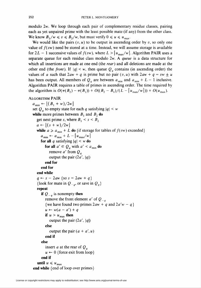
Algorithm PAIR

ûonn «- l(*l + h0/2w]set Q to empty state for each q satisfying \q\ < w

while more primes between Bx and B2 do

get next prime s, where Bx < s < B2

a <- [(s + w)/2w\

while a > amin + L do {if storage for tables of f(vw) exceeded}

ûmin«- tfmin + L-f"max/H

for all q satisfying \q\ < w do

for all a' e Qq with a' < amin do

remove a' from Qq

output the pair (2a', \q\)

end for

end for

end while

q «- s — 2aw {so s = 2aw + q )

{look for mate in Q q, or save in Qq)

repeat

if Q_ is nonempty then

remove the front element a' oi Q_q

{we have found two primes 2aw + q and 2a'w - q}

u «- w(a — a') + q

if " > "max then


else

output the pair (a + a',u)

end if

else

insert a at the rear of Qq

u *- 0 {force exit from loop}

end if

until u < wmax

end while {end of loop over primes}



for all q satisfying \q\ < w do {empty the queues}

while Qq is nonempty do

remove front element a' of Q


end while

end for. D

The queues can be implemented as linked lists. It is a property of the algorithm

that Qq and Q_ will not both be nonempty at once. If all prime divisors of 2w are

below Bx, then Qq will always be empty if GCD(<?, 2w) > 1. Therefore, the total size

of the queues will never exceed Ly(2w)/2. This can be reduced to «<p(2w)/2 where

u = [«max/wj by modifying the algorithm to remove a' from Qq before inserting a

in Q if a' < a - «, thereby assuring Q will never have over « members. Another

implementation of the queues keeps a bit pattern for each Qq, in which bit b is set to

1 if and only if amin + b e Qq, for 0 < b < L. The bit patterns must be shifted

when amin advances.

Each pair (v, u) output by Algorithm PAIR satisfies

(4.2.1) 2amin < v < 2(amn + L - 1) and 0 < u ^ ux

It is straightforward to extend the algorithm to maintain tables of f(u) and f(vw)

for all u and v satisfying (4.2.1). The operation "output the pair (v, «)" will

translate into "call TEST(/(w) - f(u)); if N = 1 then return." Here TEST is as

described in Subsection 3.3. Also initialize c «- 0 at the start of PAIR, and call

CHEK at its end. If several values of N are to be factored using the same Bx, B2, w,

L, and wmax, then Algorithm PAIR need be run only once.

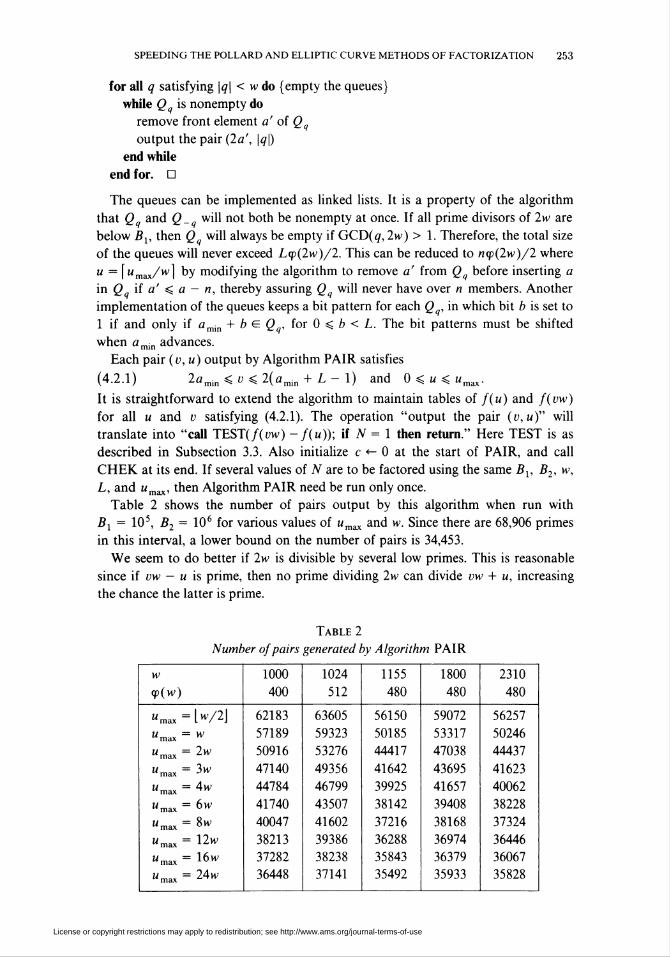
Table 2 shows the number of pairs output by this algorithm when run with

Bx = 105, B2 = 106 for various values of wmax and w. Since there are 68,906 primes

in this interval, a lower bound on the number of pairs is 34,453.

We seem to do better if 2w is divisible by several low primes. This is reasonable

since if vw — u is prime, then no prime dividing 2w can divide vw + u, increasing

the chance the latter is prime.

Table 2

Number of pairs generated by Algorithm PAIR

w

cp(w)

1000

400

1024

512

1155

480

1800

480

2310

480

"max = 3w

"max=iW/2j

W

2w

3w

"max = 4w

"max = 6W

"max - 8W

"max = 12W

"max = 16*"

"max = 24W

62183

57189

50916

47140

44784

41740

40047

38213

37282

36448

63605

59323

53276

49356

46799

43507

41602

39386

38238

37141

56150

50185

44417

41642

39925

38142

37216

36288

35843

35492

59072

53317

47038

43695

41657

39408

38168

36974

36379

35933

56257

50246

44437

41623

40062

38228

37324

36446

36067

35828



5. Lucas Functions. Let P be an element of a commutative ring with identity

(normally the integers modulo N). For each integer «, define the Lucas functions

Un= Un(P) and Vn=Vn(P)hy

£/0 = 0, Ux = l, U„+x = PUn-U„_x,

V0 = 2, VX = P, Vn + l = PVn-V„_x.

Also define A = A(F) = P2 - 4. If x2 - Px + 1 = (x - a)(x - ß), and if divi-

sion by a - ß is allowed, then

Un(P) = (a"-ß")/(a-ß), Vn(P) = a" + ß", t\{P) = (a - ß)\

These functions satisfy many identities [14], [33] (the argument P will be omitted

when it is clear from the context):

£/_„ - - U„, V_n = Vn, U2n = UnVn, V2n = V2 - 2, V2 - AU2 = 4,

(5.1) 2Um+n = UmVn + V„fJn, 2Vm+n = VmV„ + AUmUn,

V = V V - V

1 } Vmn(P) = Vm(V„(P)),

(5.3) {Vm+n-2)(Vm_n-2) = (Vm-Vn)2-

Theorem 1. If p is an odd prime and P is an integer and the Legendre symbol

(A(P)/p) = e + 0, then Vm(P) = Vn(P) mod p wheneverp - e\m + n.

Proof. If m = 0 or n = 0, see [14, p. 423]. Otherwise use Eq. (5.3). D

One can compute U„(P) and Vn(P) from « and P with 0(log«) operations [18],

[33].In Subsection 4.1, we used /(«) = b"~ mod N. Another acceptable selection is

f(n) = b" + b~" = Vn(b + b~l) mod TV.

This is well defined since GCY)(b,N) = 1. This selection of / requires only one

multiplication modulo TV to compute each successive value of f(vw) or f(u), by

(5.2). It also leads to compatibility with the p + 1 method of factoring.

6. The p + 1 Method of Factoring. Williams's p + 1 method of factoring [33]

assumes N is an integer to be factored and p is an unknown prime factor of N for

which p + 1 has only small prime factors. Pick an integer P0 other than 0, +1, +2.

As in the p — 1 method, pick bounds 0 «: Bx «: B2. Compute P' = VR(P0) mod N,

where R > 0 is divisible by all prime powers below Bx. If GCD(F' - 2, N) = I,

then Step 1 of the p + 1 method has been unsuccessful.

The hope is that P0 = a + a1 for some a e GF(p2) - GF(p); this will hold if

A(P0) = P02 - 4 is a quadratic nonresidue modulo p. In that case, a and a"1 will be

algebraic conjugates, implying aä = 1. The multiplicative subgroup of GF(p2)

satisfying this equation has order p + 1, so this method succeeds if A(.P0) is a

quadratic nonresidue and p + 1 is highly composite.

Williams gives a continuation similar to the standard continuation of the p - 1

method and requiring about 5(-n(B2) - ^(B^)) multiplications modulo N and GCDs

with N. Instead, by Theorem 1, if e = (A(P0)/p), and p - e = Qs where Q\R, then

Vm(P') = VmR(P0) = VnR(P0) = Vn(P') modp



whenever 5 divides m + n. We can now apply the methods of Subsection 4.1, using

/(»)- Vn(P')modN.

If the p - 1 and p + 1 algorithms are run on the same N, we hope e = -1 in the

p + 1 method, but that condition seems impossible to check beforehand. Should

e = +1, then the p + 1 method finds p when the p - 1 method would have

succeeded. Observe that the algorithm may be a p - 1 method for some primes

dividing N and a p + 1 method for others; it is really a p - (A//>) method.

Therefore [33, p. 229], the p + 1 algorithm must normally be tried using multiple

values of P0, although Algorithm PAIR need be done only once. If little is known

about the factors of N, I suggest P0 = 2/7 mod TV, so that A = -192/49 mod N

and (A//)) = (-3/p) for all p > 1. Then p - (A/p) will be divisible by 6. This

should find pif3\p — l when /» — 1 is highly composite, or if 3\p + 1 when p + 1

is highly composite. An alternate selection is P0 = 6/5 mod N, in which case

A = - 64/25 mod TV, and p - (A//?) is divisible by 4. In practice, one can try p + 1

once or twice before switching to ECM.

7. Elliptic Curves. Let K be a field of characteristic other than 2 or 3. An elliptic

curve over K is the set of points (x, y) & K X K satisfying the Weierstrass equation

(7.1) y2 = x3 + Ax + B,

where A, B e K and 4A3 + 2752 =£ 0. These points plus a point at infinity form an

Abelian group when addition is suitably defined [32, p. 181]. The identity element of

the group is the point at infinity, and the negative of (x, y) is (x, —y).

Four cases arise when adding two points. If either is the identity, then their sum is

the other point. If the points are negatives of one another, then their sum is the

identity. If Px = (xx, yx) and P2 = (x2, y2) are two points on the curve where

xx + x2, and neither is the identity, then their sum is P3 = (x3, y3) where

™ = (y2~ yx)/(x2- xx), x3 = m2 - xx - x2,

y3 = m(xx - x3) -yx = m(x2 - x3) -y2.

Here m is the slope of a straight line passing through Px, P2, and —P3. The

remaining case occurs when xx = x2 but yx =t —y2. By (7.1), this implies yx = y2, so

the points are identical; one can use m = (3x2 + A)/(2yx) (the slope of the tangent

line), with the above equations for x3 and y3.

If K = GF(p) where p is prime, then the order of the group is between

p + 1 - 2\fp and p + 1 + 2\fp [32, p. 187] but varies with A and B. A major

strength of ECM is that different curves are unlikely to have equal group orders, so

ECM can be repeated (with a different curve) when it fails.

D. V. Chudnovsky and G. V. Chudnovsky [8, Section 4] give several alternative

parametrizations of elliptic curves.

8. The Elliptic Curve Method of Factoring. Lenstra's elliptic curve method of

factoring [15], [16] notes that although the ring of integers modulo N is not a field,

unless N is prime, the same algebraic operations used to add two points over a field

may be used in the ring until a noninvertible denominator is encountered. At that

time, we will usually get a factor of N. He begins with a random elliptic curve and a

random point P0 = (x0, y0) on the curve. We hope N = pq where the order of the



group modulo p (and hence the order of P0) has only small prime divisors. So

compute P' = RPq = (xx, yx), where R is divisible by all primes below our bound

Bx. If all denominators are invertible, then Step 1 of ECM has been unsuccessful.

Lenstra does not suggest a continuation. The methods of Subsection 4.1 are

applicable if we set /(«) = x„ mod N, where nP' = (xn, yn). With this selection, the

costs of Step 2 in the p ± 1 methods and ECM are essentially equal.

9. Other Continuations to p ± 1 and Elliptic Curve Methods.

9.1. Avoiding a Table of Primes. Pollard's FFT continuation to the p - 1 method

can be viewed as follows. Let

ÍS, = {¿>"mod/V:0< u < w and GCD(M,w) = 1},(9 11)v ' ' ' \S2= {bowmodN: [Bx/w\ < v ^\B2/w]).

Then check if GCD(i1 - s2,N)> 1 for some sx e Sx and s2 e S2. The algorithm

of Subsection 4.1 can be viewed in this perspective if it is changed to test all

differences f(vw) — f(u), not just those for which vw + u or vw - u is prime and

(v, u) is in our list. Define

jSx = {f(u) mod N:0 ^u^ w/2 and GCD(w, w) = 1},

\S2= {f(vw) mod N: \Bx/w - \\ < v < [B2/w + j]}.

The two sets called S2 have comparable sizes, but Sx in (9.1.2) is only half as large

as Sx in (9.1.1).

Sets Sx and S2 in (9.1.2) have the form S] = f(Dx) mod N and S2=f(D2)

mod N, where Dx and D2 are sets of integers, and where every prime between Bx

and B2 divides some nonzero element of Dx ± D2. In (9.1.2), D2 is an arithmetic

progression, and Dx is almost one but has selected terms omitted. We can reduce

IDJI-DjI (the potential number of comparisons) while keeping both \DX\ and \D2\

(and hence total memory) small, by using two sieves rather than one. Select two

coprime moduli wx and w2 such that wxw2 <s: B2 is divisible by many low primes. Set

vi = [^1/^2 — wi/2] and v2 = [B2/w2 + wx/2\. Let

I Dx = {uwx:0 < u < w2/2andGCD(w,w2) = 1},

(D2= {vw2: vx < v < v2 and GCD(v,wx) = 1}.

Another interesting choice is

Dx = {2Jm:0^j < 2J), D2= {2/m3/cm: 0 < k < K}

for positive integers «1, J and A^ where (7 + 1)(A" + 1) > (B2 - l)/2. These \DX\

and \D2\ are much larger than those in (9.1.3), since no sieving has been done, but

any odd prime s will divide some nonzero element of Dx + D2 if 5 — 1 <

B2GCD((s - l)/2,m), not merely if s < B2. Many primes greater than B2 will

qualify, even some greater than mB2. We are applying a miniature p - 1 algorithm

in our search for s. Here, Dx and D2 are geometric rather than arithmetic

progressions, so (4.1.3) does not apply, but all members of f(Dx) and f(D2) can be

evaluated with 2m(J + K) multiplications modulo N if f(n) = Vn(P').

Brent [5] suggests a "birthday paradox" continuation, in which Dx = D2. Its

elements are selected randomly, and one hopes for duplicates modulo 5.



Define the polynomials (/ = 1,2)

hl(x) = U(x-s,)modN (s,eSt).

We need the resultant of hx and «2 (or of hxh2 and its derivative). Schwartz [26, pp.

705-707] gives an asymptotically fast resultant algorithm. There is a danger that

multiple factors of N will appear at once if a single GCD with N is done at the end

of the resultant computation.

Another possibility is to evaluate GCD(hx(s2),N) for each s2 e S2. The FFT

continuation uses this approach, taking advantage of the fact that S2 in (9.1.1) is a

geometric progression, a property not shared by S2 in (9.1.2). But a polynomial of

degree at most « - 1 can be evaluated at « points in 0(«(log«)2) steps using other

FFT algorithms [1, Chapter 8]. It remains to be determined whether this extra factor

of log« will offset the reduced size of Sx when Bx and B2 are in the range of

interest.

Alternatively, we can precondition the coefficients of hx, as in Subsection 3.1, so it

can be evaluated at an arbitrary s2 e S2 with about \ deg «, multiplications modulo

N, for a total cost of about \ deghxdegh2 = \ \SX\\S2\ multiplications. Another way

to precondition using only rational operations appears in [1, Exercise 12.36]; add the

condition ru = m - I + 1 to its description.

9.2. Using f(n) = Vg{n)modN. If / satisfies the second condition of Subsection

4.1 (with p - 1 = Qs replaced by an appropriate group equation), then so does F

where F(n) = f(g(ny) and where g is an odd or even polynomial function with

integer coefficients. This is because if s divides either vw + u, then s will divide one

of g(vw) + g(u). The advantage to using F is that a prime s > B2 may divide

g(vw) + g(u) even though 5 divides neither vw + u. This increases our chances of

finding s and hence p, at the cost of increased time to compute values of F(vw) and

F(u). If deg g > 1, then our s might divide F(vw) — F(u) when vw ± u are both

composite, so this becomes more attractive when using one of the methods in

Subsection 9.1. I suggest g be chosen so g(x) ± g(y) have many algebraic factors,

such as g(x) = x" where « has many divisors.

This approach requires evaluating / at points x, x + h, x + 2«,... of an arith-

metic progression. For ECM, we can compute g(n)P as in (4.1.3) (unless we are

using the alternative parametrization of Subsection 10.3.1). For the p - 1 method of

factoring, successive values of Vg{n) can be found by separately computing

¿>g<n) mod N and b~s(n) mod /V in this manner. For the p + 1 method, let d = deg g.

Define g¡ for 0 < / < d by (4.1.3). If we know Vg{n)/2modN and Ug{n)/2mod N

for 0 < / < d, then 5d multiplications modulo N suffice to replace « by « + «, by

(5.1). Another method defines

A' = ( A - X2 )/4X2 mod N, Wk = ( Vk + XUk )/2 mod N,

where À is arbitrary except that GCD(A, N) = 1. Then

Vk = Wk + W_k mod N, XUk =Wk- W_k mod N,

wJ+k= WjWk + A'\2UjUk mod N, W_J_k = W_JW_k + K\2UJUk mod N.

For 0 < i < </, keep track of W±g(n)modN and c,t/g(n)mod/V where c, =

XA'mod N if / is even and c¡ = A mod A if i is odd. Then [3.5^] multiplications

modulo N suffice to replace « by « + «.



9.3. Can We Pair More than Two Primes! If Algorithm PAIR is replaced by an

algorithm which generates triplets of primes, and if / is changed accordingly, then

the algorithm in Subsection 4.1 will be speeded up 33%. I have been unable to do

this.

If f(x) - f(y) divides f(xn) - f(yn) whenever x, y, and « are integers, then

GCD(f(xxx2) -f(xxy2) -f(yxx2) +f(yxy2),N)

can be tested instead of separately testing

GCD(f(xx)-f(yx),N) and GCD(f(x2) - f(y2), N).

If the pairs of primes can themselves be paired for this computation, then the

number of GCDs with N will drop by half. This seems to require evaluating / at too

many points to be worthwhile.

10. Implementations. The author is preparing a table of factorizations [7] of

Fibonacci numbers Fn for odd « < 999, and of Lucas numbers L„ for « < 500.

Those tables were the primary testing grounds for these algorithms.

If p > 5 is an odd primitive prime factor of Fn or Ln (meaning p\Fn (respectively

p\Ln) but p + Fk and p 1 Lk if 0 < k < «), then p = (5/p) = (p/5) mod2«. If

51«, then p = 1 mod 2«. Otherwise, we merely know p = +1 mod 2«.

Let A be a composite cofactor of a Fibonacci or Lucas number. The author found

approximately 180 new factors of such N between 1983 and 1985, using these

algorithms on primarily a VAX 11/780 and a CDC 7600. The Monte Carlo method

was tried on approximately half of the entries, usually for about 30,000 function

evaluations. Meanwhile either p - 1 or p + 1 was run against the same input

number. Monte Carlo was less productive than p + 1, and was abandoned once

ECM was implemented. The elliptic curve and p + 1 methods were run on all

composite entries in the tables. The programs used a variation of the algorithm in

[17]* for arithmetic modulo N.

10.1. Implementations of p + 1. The p - 1 and p + 1 methods were tried on each

N, using increasing limits and various seeds. Williams [33] and Naur [19] had

previously tried these methods. Most runs were made before ECM was discovered.

The first and last runs of p + 1 used P0 = 23/11 mod N. Since A = F02 - 4 =

45/121 mod A is 5 times a rational square, this will locate a factor p of N if

p — (5/p) is highly composite. However p — (5/p) is known a priori to be divisible

by 2«.

The last p + 1 run used Bx = 2,000,000 and B2 = 100,000,000. Equation (9.1.3)

was used with wx = 221 and w2 = 2310. It used /(«) = V{n)(P'), where

g(«) = V6(n) = «6 - 6«4 + 9«2 - 2.

We wrote hx (of degree 2q>(w2) = 240) as a product of 16 monic polynomials each

of degree 15, and expanded each of the latter using Winograd's scheme (3.1.2). It

took 21 multiplications modulo N to compute each value of f(vw2), and an

additional 130 multiplications modulo N and one GCD with N to evaluate

GCD(hx(f(vw2)), N) if GCD(i;, 221) = 1.

'Robert Baillie has kindly pointed out an error in [17], In the fifth line of Section 2 on p. 520, change

"modulo R" to "modulo b". Also change "/?" to "b" in the first statement within the for loop on p. 520.


SPEEDINC; THE POLLARD AND ELLIPTIC CURVE METHODS OF FACTORIZATION 259

The use of /(«) = Vg(n) rather than /(«) = Vn occasionally produces surprises,

such as the factor 124,205,327,610,431 of 3281 - 1 despite B2 = 2,000,000, be-

cause 21,488,179 (the only large divisor of p - 1) also divides F3(2310 • 516) +

J/3(221 • 733). Such successes seem rare, and did not occur during the final p + 1

run on the Fibonacci and Lucas numbers.

The largest factors found by p ± 1 were

142,240,444,249,423,907,190,721 of F537,

6,563,589,514,883,537,474,323,387 of LM2,

619,802,607,259,514,583,330,235,693,729 of F971,

for which

p - 1 = 26 • 3 • 5 • 72 • 23 • 179 • 1693 • 6311 • 68741623 (F537),

p + 1 = 22 • 13 • 17 • 47 • 2459 • 69029 • 255877 • 3637223 (L442),

p - 1 = 25 • 3 • 13 • 23 • 971 • 25801 • 689851 • 1089469 • 1146793 (F971).

The 30-digit factor of F971 was found in Step 1. Silverman found a 26-digit factor of

L431 via p - 1.

10.2. Implementation of Monte Carlo. Brent and Pollard [4] recommend F(x) =

x m + 1 if the factors of N are known to be congruent to 1 modulo m. They demonstrate

by finding the previously unknown factor 1,238,926,361.552,897 of 2256 + 1 using

m = 1024. Use of this polynomial seems to reduce the expected number of function

evaluations before finding a prime p by (GCD(p - 1, m) - 1)1/2. Gold and Sattler

[11] report a similar result, without the second " -1" term.

When 5|«, we used F(x) = xm + I. The selection of m was sometimes 120«,

sometimes 5040«, and sometimes 16 • 9 • 5 • 7 • 11 ■ 13«.

For the case where 5 + «, consider F(x) = Vm(x) + c where 2«|w. Let p be a

prime satisfying p = ±1 mod 2«. An argument resembling that in [4] suggests that

this reduces the expected number of function evaluations before finding p by a

factor of

((GCD(p - l,m) + GCD(p + I, m) - 2)/2)1/2 > ((2« + 2 - 2)/2)1/2 = y/n .

To utilize Algorithm MCF of Subsection 3.2, we can rewrite F as

(10.2.1) F(x) = Vm/2(V2(x)) + c = Vm/2(x2 - 2) + c = G(*2),

where G(x) = Vm/2(x — 2) + c. Actually, we used F(x) = Vm/2(x2), with m as in

the 5|« case. Algorithm CFRC of [18] was used (along with the factorization of

m/2) to find a fast way to evaluate F(x).

The author found only ten Fibonacci and Lucas factors with this algorithm before

abandoning it in favor of ECM. The largest such factor was 17,672,296,363,133,261

of F893.

10.3. Effectiveness of ECM. The author ran ECM several times, using approxi-

mately 50 total curves for each N. In Step 2, /(«) is the x-coordinate of nP.

ECM found over 100 factors missed by other methods (albeit using considerably

more computer time). The largest Fibonacci and Lucas factors found by ECM were

2,442,882,935,400,038,849,127,521 of F517,

10,245,029,712,795,120,034,405,043 of L386,

12,158,771,296,959,377,863,294,133 of F563,

5,890,430,821,204,665,088,535,469,913 of F869.


260 PETER L MONTGOMERY

The factor of L386 was found with Bx = 106; for the others, Bx was between

50000 and 100000. In each case, B2 was about 60 times as large.

The author subsequently implemented the parametrization in Subsection 10.3.1,

and tackled twenty-five composite entries of the form 12" + 1 from [6]. Previous

ECM runs, primarily by Silverman, had removed their small factors. Using ap-

proximately 80 curves per number, with Bx varying from 100000 to 500000, I found

eleven new factors of 20 to 24 digits, but was disappointed to find no larger ones.

After two partially factored entries were completed by Silverman using the methods

of [30], seventeen composite entries of 76 to 136 digits remained. Silverman's runs

revealed I had missed a 22-digit factor of 1273 + 6 • 1236 + 1.

The author then returned to the Lucas numbers, using the parametrization in

Subsection 10.3.1. He found three huge factors:

1,090,414,335,383,168,463,561,145,167,623 of L412,

5,373,430,329,122,468,821,883,671,012,169 of L482,

227,693,725,298,545,340,302,283,668,318,476,481 of L464.

Both 31-digit factors were found using Bx = 175000. The 36-digit factor was found

using Bx = 225000. In each case, B2 was 40 times as large as Bx.

10.3.1. Elliptic Curve Parametrization. The author's original implementation of

ECM used affine coordinates, as in (7.1). Adding two points takes 2 multiplications,

6 additions, and 1 division when the points are distinct, and slightly more when they

are equal. Each division requires a multiplication and an inversion. When working

over several curves, the program used a scheme similar to (1.2) to do all the

inversions at once, since (l/x) = y(l/xy) and (l/y) = x(l/xy). This reduces the

asymptotic cost of an inversion to that of 3 multiplications. If one uses a method

requiring log2« duplications of points and 0.25 log 2« additions or subtractions of

points when computing nP from P, then the asymptotic cost of this method is about

(7 + 6(0.25)) log2« = 8.5 log 2« multiplications per curve. However, one must run

several curves at once to achieve this performance. Furthermore, this inversion

algorithm is not suitable for parallel or distributed processing.

The author later discovered an alternative parametrization that requires no

inversions during Step 1, once the necessary constants have been computed. It

resembles (4.18i) and (4.18ii) in [8] and uses the equation

(10.3.1.1) By2 = x3 + Ax2 + x

for some A and B.

Let Px = (xx, yx) and P2 = (x2, y2) be two points on the curve, with xx # x2 and

xxx2 =é 0. Then Px + P2 = (x3, y3) satisfies

*3 = B[(yi -yi)/(xx - x2)}2 - a - xx - x2,

*s(*i - *2)2 = B(yi -y2? ~(A + xx + x2)(xx - x2)2

= -2Byxy2 + xxx2(xx + x2 + 2A) + xx + x2

= B(x2yx - xxy2)2/xxx2.

Similarly, Px - P2 = (x4, y4) satisfies

xA(xx - x2)2 = B(x2yx + xxy2)2/xxx2.



Multiply these equations and use (10.3.1.1) to obtain

x3x4(xx - x2)2 = (xxx2- I)2

after division by (xx - x2)2. This equation remains valid if xxx2 = 0. If Px = P2, a

similar derivation yields

4xxx3{x2 + Axx + l) = (x2 - l) .

These equations reference only the x¡, not the y¡. Fortunately, ECM does not

require us to compute the y¡.

Let P be an arbitrary point on the curve, and let the x-coordinate of nP be the

rational number XJZn. From the ratios (Xm_n: Zm_„), (Xm:ZJ, and (Xn:Zn),

one can compute the ratio (Xm+n : Zm+n) via the addition formula

if mP ¥= nP, and via the duplication formula

X2n +-{X¿- Z2)2, Z2n «- 4*„Z„(*2 + AX„Zn + Z2)

if m = n. The addition formula is valid everywhere if we allow GCD(Xn, Z„, N) to

exceed 1. Once that condition occurs, it will persist, so we can periodically test

GCD(Z„, A).

The addition formula seems to require 8 multiplications and the duplication

formula to require 6 multiplications. The costs drop if we store the ratios

(Xm:Zm: Xm + Zm:Xm- Zm) and rewrite the formulae as (the right sides of the

addition formula have been multiplied by 4)

xm+n *- Zm_„[(Xm - Zm)(Xn + z„) +(xm + zm)(x„ - z„)]2,

Zm+„ *~ Xm_n[(Xm — Zm)(X„ + Zn) —\Xm + Zm)(Xn — Zn)\ ,

and

4xnzn = (xn + zn)2-(x„- z„)2, X2„ ̂ (X„ + Zn)\Xn - zn)\

Z2n *- (4X„Z„){(X„ - Z„)2+((A + 2)/4)(4X„Z„)).

Note that we can precompute (A + 2)/4. These formulae require 6 multiplications

and 4 additions to add two points whose difference is known, and 5 multiplications

and 4 additions to duplicate a point.

Using the binary method, we can compute nP from P with 11 log 2« multiplica-

tions and 81og2« additions, by repeatedly computing either (2mP, (2m + l)P) or

((2m + l)P, (2m + 2)P) from (mP, (m + l)P). If one starts with Xx = 2 and

Zx = 1, then this cost reduces to 9 log 2 « multiplications and 9 log 2 « additions.

We can do almost as well for arbitrary Xx and Zx by noticing that these equations

functionally resemble (5.2). The methods of [18] may be used to evaluate «F from P

with about 1.55 log2« addition or duplication steps, which corresponds to about

9.3 log2 « multiplications and 6.2 log2 « additions. In practice, both this method and

the binary method (with Xx/Zx = 2) use about 130,000 multiplications for Step 1 to

reach 10,000. The binary method has a simpler control structure and a greater

percentage of squarings (44% vs. 34%) but requires 45% more additions. In the

binary method, 11% of the multiplications can be replaced by additions if (A + 2)/4

is sufficiently small.



One can use this parametrization during Step 1 and the Weierstrass parametri-

zation during Step 2, by arbitrarily setting y = 1 at the end of Step 1, using

(10.3.1.1) to compute B, and applying a linear transformation to obtain (7.1).

10.3.2. Selection of Elliptic Curves and Initial Points. ECM lets one pick which

curve to use. Naturally, one prefers a curve whose group order has some known

prime divisors, since the group order is more likely to be highly composite. When

using the Weierstrass equation (7.1), each linear factor x - x0 of x3 + Ax + B

corresponds to a point (x0,0) of order 2 on the curve. If the cubic has three linear

factors, then the group will have a subgroup isomorphic to Z2 X Z2. Therefore, the

group modulo each prime divisor of A will have order divisible by 4. For example,

one can select three distinct squares s2, s2, and s2, and use the point

(xi,yi) = {{sx + s\ + s2)/3, sxs2s3)

on the curve

(x + s¡ - xx)(x + s¡ - xx)(x + s¡ - xx) = y2.

When using (10.3.1.1), it is desirable to use B = A + 2 so that the point (1,1) will

have order 4. We also desire A = k + l/k for some k, so that there will be three

points of order 2. We can achieve both of these (and hence have a group order

divisible by 8) providing we can select xx = Xx/Zx where (k + xx)(k + l/xx) is a

perfect square. This will hold if k = (x2 - m2)/(xx(m2 - 1)) for some m. To

prevent degenerate cases such as division by zero, and to ensure that our starting

point is not in the known subgroup, one needs

mxx(x2 - l)(m2 - l)(x2 - m2)(x2 - m4) * 0.

In particular, we can select xx = 2 and m = 3,4,5,_

When -1 is a quadratic residue, we can obtain a curve whose group order is

divisible by 16 if we do not insist that xx = 2. The point (x, y) has order 4 if

x2 + 2kx + 1 = 0 and (1 + k)y2 = (1 - k)x2. Such a rational point exists if -1

and k2 - 1 are quadratic residues. The latter condition holds if (x2 — l)(x\ - m4)

is a perfect square. One nontrivial solution is xx = m2 + 2 where m = (t2 - 3)/2i

for t = 4,5,6,_

Let p be a prime which does not divide B(A + 2)(A - 2). Suyama [31] observes

that the order of the group associated with (10.3.1.1) modulo p will always be

divisible by 4. If B(A + 2) is a quadratic residue, then the point (1, \/(A + 2)/B)

has order 4. If B(A - 2) is a quadratic residue, then the point (-1, \j(A - 2)/B)

has order 4. If (A + 2)(A - 2) is a quadratic residue, then the cubic has three linear

factors, and again there is a subgroup of order 4.

Suyama next notes that if

A = (-3a4 - 6a2 + l)/4a3, B = (a2 - l)2/4ab2,

where a, b e Q and ab(a2 - l)(9a2 - 1) + 0, then the point (a, b) has order 3,

implying the group order is divisible by 12. It remains to select i^we require that

4a3x3-(3a4 + 6a2 - l)x2 + 4a3xx



be a perfect square. Suyama suggests xx = 3a/4, where 9 - 6a2 is a perfect square

(e.g., a = 6u/(u2 + 6) where u is rational). Alternative initial points are xx = a3

where 4a2 + 5 is a perfect square, and xx = (3a2 + l)/4a, where 3a2 + 1 is a

perfect square.

There will be a torsion group of order 12 over Q if (1 - a)(l + 3a), and hence

B(A + 2) is a perfect square. Set a = (u2 - 4« - 12)/(w2 + 12w - 12); then both

3a2 + 1 and (1 - a)(l + 3a) will be perfect squares whenever u3 - 12« is a perfect

square (e.g., u = 4, 54, 49/4, 2166/625, 14884/1089). Avoid u = 0, - 2, 6 since

they lead to degenerate cases. The explicit torsion group seems to give a 50% chance

that B(A + 2), B(A - 2) and (A - 2)(A + 2) will all be quadratic residues (ensur-

ing the group order is divisible by 24), compared with a 25% chance if we know

nothing about A and B.

Acknowledgments. D. H. Lehmer provided me with a copy of his multiprecision

arithmetic package. H. C. Williams and Robert Silverman verified the primality of

many of the cofactors found. Andrew Odlyzko sent me [8] and [15]. My colleagues

gave their support and encouragement while this work was in progress. System

Development Corporation provided extensive, otherwise idle, computer time, and a

Versatec printer plotter. Mike Mitchell and Richard Milton spent many hours

running jobs on a CDC 7600. Without the Engineering and Mathematical Sciences

Library at the University of California, Los Angeles, this research could not have

been accomplished.

System Development Corporation

2525 Colorado Avenue

Santa Monica, California 90406

1. Alfred V. Aho, Iohn E. Hopcroft & Jeffrey D. Ullman, The Design and Analysis of Computer

Algorithms, Addison-Wesley, Reading, Mass., 1974.

2. Sara Baase, Computer Algorithms: Introduction to Design and Analysis, Addison-Wesley, Reading,

Mass., 1983.3. Richard P. Brent, "An improved Monte Carlo factorization algorithm," BIT, v. 20, 1980, pp.

176-184.4. Richard P. Brent & John M. Pollard, "Factorization of the eighth Fermât number," Math.

Comp., v. 36,1981, pp. 627-630.5. R. P. Brent, "Some integer factorization algorithms using elliptic curves," presented to Australian

Computer Science Conference, ACSC-9,1986.

6. John Brillhart, D. H. Lehmer, J. L. Selfridge, Bryant Tuckerman & S. S. Wagstaff, Jr.,

Factorizations of b" + 1, b = 2,3,5,6,7,10,11,12 Up to High Powers, Contemp. Math., vol. 22, Amer.

Math. Soc„ Providence, R. I., 1983.

7. John Brillhart, Peter L. Montgomery & Robert D. Silverman, "Tables of Fibonacci and

Lucas factorizations." (In preparation.)

8. D. V. Chudnovsky & G. V. ChudnOVSKY, Sequences of Numbers Generated by Addition in Formal

Groups and New Primality and Factorization Tests, Research report RC 11262 (#50739), IBM Thomas

J. Watson Research Center, Yorktown Heights, N. Y., 1985.

9. James A. Davis & Diane B. Holdridge, Most Wanted Factorizations Using the Quadratic Sieve,

Sandia report SAND84-1658, August, 1984.10. Joseph L. Gerver, "Factoring large numbers with a quadratic sieve," Math. Comp., v. 41. 1983, pp.

287-294.11. R. Gold & J. Sattler, "Modifikationen des Pollard-Algorithmus," Computing, v. 30, 1983, pp.

77-89.12. Richard K. Guy, "How to factor a number," Congressus Numerantium XVI, Proc. Fifth Manitoba

Conf. on Numerical Math., Winnipeg, 1976, pp. 49-89.



13. DONALD E. Knuth, The Art of Computer Programming, Vol. II, Seminumerical Algorithms, 2nd

ed., Addison-Wesley, Reading, Mass., 1981.

14. D. H. Lehmer, "An extended theory of Lucas' functions," Ann. of Math. (2), v. 31, 1930, pp.

419-448.

15. H. W. Lenstra, Jr., "Elliptic curve factorization," announcement of February 14,1985.

16. H. W. Lenstra, Jr., "Factoring integers with elliptic curves." (To appear.)

17. Peter L. Montgomery, "Modular multiplication without trial division," Math. Comp., v. 44,1985,

pp. 519-521.18. Peter L. Montgomery, "Evaluation of Vn(P, 1) via Lucas chains," Fibonacci Quart. (Submitted.)

19. Thorkil Naur, "New integer factorizations," Math. Comp., v. 41, 1983, pp. 687-695.

20. M. A. Morrison & J. Brillhart, "A method of factoring and the factorization of F7," Math.

Comp., v. 29,1975, pp. 183-208.21. J. M. Pollard, "Theorems on factorization and primality testing," Proc. Cambridge Philos. Soc, v.

76,1974, pp. 521-528.

22. J. M. Pollard, "A Monte Carlo method for factorization," BIT, v. 15,1975, pp. 331-334.23. J. M. Pollard, private communication.

24. Hans Riesel, Prime Numbers and Computer Methods for Factorization, Birkhäuser Progress in

Mathematics, vol. 57, Boston, 1985.

25. C. P. Schnorr & H. W. Lenstra, Jr., "A Monte Carlo factoring algorithm with linear storage,"

Math. Comp., v. 43,1984, pp. 289-311.26. J. T. Schwartz, "Fast probabilistic algorithms for verification of polynomial identities," /. Assoc.

Comput. Mach., v. 27, 1980, pp. 701-717.27. R. Sedgewick & T. G. Szymanski, The Complexity of Finding Periods, Proc. Eleventh Annual

ACM Symposium on Theory of Computing, ACM, New York, 1979, pp. 74-80.

28. Daniel Shanks, Class Number, a Theory of Factorization, and Genera, Proc. Sympos. Pure Math.,

vol. 20, Amer. Math. Soc, Providence, R. I., 1971, pp. 415-440.29. Robert D. Silverman, private communication.

30. Robert D. Silverman, "The multiple polynomial quadratic sieve," Math. Comp., v. 48, 1987, pp.

329-339.31. Hiromi Suyama, "Informal preliminary report (8)," 25 Oct. 1985.

32. John T. Täte, "The arithmetic of elliptic curves," Invent. Math., v. 23,1974, pp. 179-206.

33. H. C. Williams, "Ap + 1 method of factoring," Math. Comp., v. 39,1982, pp. 225-234.

34. H. C. Williams, private communication.

35. S. Winograd, "Evaluating polynomials using rational auxiliary functions," IBM Technical Dis-

closure Bulletin, v. 13, 1970, pp. 1133-1135.


Speeding the Pollard and Elliptic Curve Methods of Factorization · Speeding the Pollard and...

Documents

Transcript of Speeding the Pollard and Elliptic Curve Methods of Factorization · Speeding the Pollard and...