H. Wang, J. Li, Q. Y. Chen and D. Ni 1

Speed-Density Relationship: From Deterministic to StochasticHaizhong WANG (Corresponding Author)Department of Civil and Environmental EngineeringUniversity of Massachusetts Amherst142D Marston Hall130 Natural Resources RoadAmherst, MA 01003Email: wang@engin.umass.edu

Jia LIDepartment of Civil and Environmental EngineeringUniversity of Massachusetts Amherst142D Marston Hall130 Natural Resources RoadAmherst, MA 01003Email: jli0@engin.umass.edu

Qian-Yong CHEN, Ph. DDepartment of Mathematics and StatisticsLederle Graduate Research TowerUniversity of MassachusettsAmherst, MA 01003-4515Phone: +1 413 545-9611Fax: +1 413 545-1801Email: qchen@math.umass.edu

Daiheng NI, Ph. DDepartment of Civil and Environmental EngineeringUniversity of Massachusetts Amherst219 Marston Hall130 Natural Resources RoadAmherst, MA 01003Phone: +1 413 545-5408Fax: +1 413 545-9569Email: ni@ecs.umass.edu

Resubmitted to TRB 88th Annual Meeting at Washington D. C. Jan. 2009Number of words: 4500Number of figures and tables: 10 (10 x 250 = 2500)Total: 7000

H. Wang, J. Li, Q. Y. Chen and D. Ni 2

Abstract

Traffic flow is a many-car system with complex and stochastic movement. It is difficult todescribe the system dynamics solely using deterministic models which describe average sys-tem behaviors. Therefore, a stochastic speed-density relationship is proposed as a further stepforward to overcome the well-known drawbacks of deterministic models. Modeling resultsshow that by taking care of second-order statistics (i.e., mean and variance) a stochastic speed-density model is suitable for describing the observed phenomenon as well as matching theempirical data. From here, a stochastic fundamental diagram of traffic flow can be established.The stochastic speed-density relationship model can potentially be used for real-time on-lineprediction and to explain phenomenons in a similar manner.

H. Wang, J. Li, Q. Y. Chen and D. Ni 3

1 IntroductionThe speed-density relationship serves as the basis to understand system dynamics in variousdisciplines. It can be used to model moving objects (or particles) in many scientific areas:pedestrians [1] [2], conveyors, network information packages [3],crowd dynamics [4], molec-ular motors, and biological systems [5]. In this paper, we focus on the fundamental speed-density relationship of vehicular traffic flow. Our goal in this paper is to propose a stochasticspeed-density relationship based on empirical ITS data (100 stations from the entire year of2003) from GA400 in Atlanta, Georgia.

In nature, deterministic models describe average system behaviors based on physical laws.In a live transportation system, a totally deterministic model is unlikely to include variousdynamical randomness effects (or uncertainties). The stochastic behavior of real-world trafficsystems is often difficult to describe or predict exactly when the influence of unknown random-ness is sizable. However, it is quite possible to capture the chance that a particular value willbe observed during a certain time interval in a probabilistic sense. In particular, speed-density(or concentration) models in a deterministic sense, whether single or multi-regimes, have a‘pairwise’ relationship; that is, given a density there exists a corresponding speed from a de-terministic formula. Empirical observations from GA400 ITS verified the existence of anotherpicture. There is a distribution of traffic speeds at a certain density level due to the stochasticnature of traffic flow, this is in contrast to the ‘pairwise’ pattern from deterministic models.There is debate on whether the scattering phenomenon observed in fundamental diagrams isdue to either the measurement errors, the inherent nature of traffic flow, or a combination of thetwo. Essentially, there are two main sources of randomness [6] [7]. The first type of random-ness is derived from the irregularity in traffic observations that come intrinsically from the datacollection system and the computational processing that follows. This can be observed fromthe scattered plots of speed-density relationships at all of the stations from GA400,refer toFig. 2. This type of randomness has been well-understood and can be controlled statistically.The second type of randomness is inherently generated by traffic dynamics, and it relates toa general lack of knowledge about what stochastic process is involved [6]. To be specific,drivers’ behaviors vary on an individual basis; the collective behaviors of driver groups wouldbe better described in distributional law rather than in deterministic terms [7]. This type ofrandomness is assumed to underly the proposed stochastic speed-density relationship referredto Fig. 1. Thus, a stochastic speed-density model is more realistic and more capable to capturethe traffic dynamics and the randomness involved in a many-car system. Before marching for-ward, it is important to mention the fundamental principles that we abide by; Herman and hiscolleagues mention that, “Traffic theory was inherently an experimental science and should bepursued as such. The second one was that the mathematical model should be chosen as the onemost suitable for describing a particular phenomenon, rather than trying to fit a phenomenonto a model particularly familiar or attractive to a researcher” [8]. Our main contributionis the proposed stochastic speed-density relationship model, its validity has been verified byempirical observations and performance compared with existing deterministic models.

2 Literature ReviewIt has been almost 75 years since Greenshields’ seminal paper Study of Traffic Capacity in1935 [9]. Attaching empirically derived curves to a fitted linear model of the speed-densityrelationship started a new era of transportation science and engineering. Due to its strong

H. Wang, J. Li, Q. Y. Chen and D. Ni 4

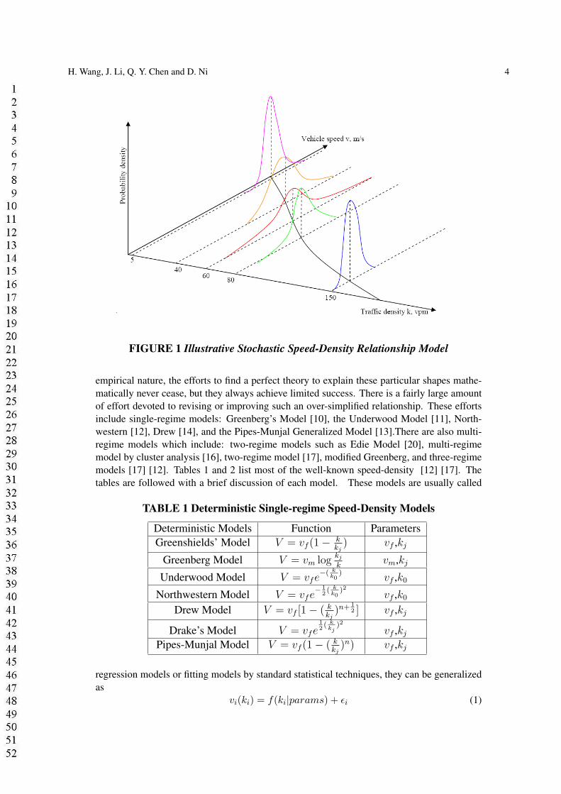
FIGURE 1 Illustrative Stochastic Speed-Density Relationship Model

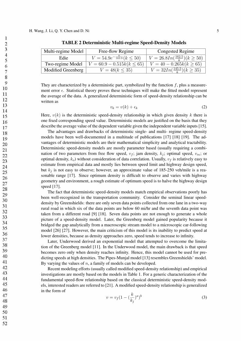
empirical nature, the efforts to find a perfect theory to explain these particular shapes mathe-matically never cease, but they always achieve limited success. There is a fairly large amountof effort devoted to revising or improving such an over-simplified relationship. These effortsinclude single-regime models: Greenberg’s Model [10], the Underwood Model [11], North-western [12], Drew [14], and the Pipes-Munjal Generalized Model [13].There are also multi-regime models which include: two-regime models such as Edie Model [20], multi-regimemodel by cluster analysis [16], two-regime model [17], modified Greenberg, and three-regimemodels [17] [12]. Tables 1 and 2 list most of the well-known speed-density [12] [17]. Thetables are followed with a brief discussion of each model. These models are usually called

TABLE 1 Deterministic Single-regime Speed-Density Models

Deterministic Models Function ParametersGreenshields’ Model V = vf (1− k

kj) vf ,kj

Greenberg Model V = vm logkj

kvm,kj

Underwood Model V = vfe−( k

k0)

vf ,k0

Northwestern Model V = vfe− 1

2( k

k0)2

vf ,k0

Drew Model V = vf [1− ( kkj

)n+ 12 ] vf ,kj

Drake’s Model V = vfe12( k

kj)2

vf ,kj

Pipes-Munjal Model V = vf (1− ( kkj

)n) vf ,kj

regression models or fitting models by standard statistical techniques, they can be generalizedas

vi(ki) = f(ki|params) + εi (1)

H. Wang, J. Li, Q. Y. Chen and D. Ni 5

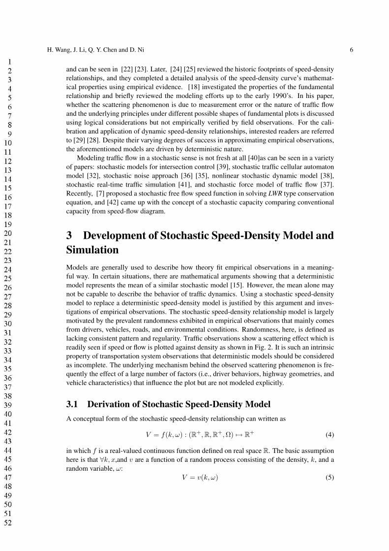
TABLE 2 Deterministic Multi-regime Speed-Density Models

Multi-regime Model Free-flow Regime Congested RegimeEdie V = 54.9e−

k163.9 (k ≤ 50) V = 26.8In(162.5

k)(k ≥ 50)

Two-regime Model V = 60.9− 0.515k(k ≤ 65) V = 40− 0.265k(k ≥ 65)Modified Greenberg V = 48(k ≤ 35) V = 32In(145.5

k)(k ≥ 35)

They are characterized by a deterministic part, symbolized by the function f , plus a measure-ment error ε. Statistical theory proves these techniques will make the fitted model representthe average of the data. A generalized deterministic form of speed-density relationship can bewritten as

vk = v(k) + εk (2)

Here, v(k) is the deterministic speed-density relationship in which given density k there isone fixed corresponding speed value. Deterministic models are justified on the basis that theydescribe the average value of the dependent variable given the independent variable inputs [15].

The advantages and drawbacks of deterministic single- and multi- regime speed-densitymodels have been well-documented in a multitude of publications [17] [18] [19]. The ad-vantages of deterministic models are their mathematical simplicity and analytical tractability.Deterministic speed-density models are mostly parameter based (usually requiring a combi-nation of two parameters from free flow speed, vf ; jam density, kj ; optimal speed, vm; oroptimal density, ko) without consideration of data correlation. Usually, vf is relatively easy toestimate from empirical data and mostly lies between speed limit and highway design speed,but kj is not easy to observe; however, an approximate value of 185-250 veh/mile is a rea-sonable range [17]. Since optimum density is difficult to observe and varies with highwaygeometry and environment, a rough estimate of optimum speed is to halve the highway designspeed [17].

The fact that deterministic speed-density models match empirical observations poorly hasbeen well-recognized in the transportation community. Consider the seminal linear speed-density by Greenshields: there are only seven data points collected from one lane in a two-wayrural road in which six of the data points are below 60 mi/hr and the seventh data point wastaken from a different road [9] [18]. Seven data points are not enough to generate a wholepicture of a speed-density model. Later, the Greenberg model gained popularity because itbridged the gap analytically from a macroscopic stream model to a microscopic car-followingmodel [26] [27]. However, the main criticism of this model is its inability to predict speed atlower densities, because as density approaches zero, speed tends to increase to infinity.

Later, Underwood derived an exponential model that attempted to overcome the limita-tion of the Greenberg model [11]. In the Underwood model, the main drawback is that speedbecomes zero only when density reaches infinity. Hence, this model cannot be used for pre-dicting speeds at high densities. The Pipes-Munjal model [13] resembles Greenshields’ model.By varying the values of n, a family of models can be developed.

Recent modeling efforts (usually called modified speed-density relationship) and empiricalinvestigations are mostly based on the models in Table 1. For a generic characterization of thefundamental speed-flow relationship based on the classical deterministic speed-density mod-els, interested readers are referred to [21]. A modified speed-density relationship is generalizedin the form of

v = vf (1− (k

kj)a)b (3)

H. Wang, J. Li, Q. Y. Chen and D. Ni 6

and can be seen in [22] [23]. Later, [24] [25] reviewed the historic footprints of speed-densityrelationships, and they completed a detailed analysis of the speed-density curve’s mathemat-ical properties using empirical evidence. [18] investigated the properties of the fundamentalrelationship and briefly reviewed the modeling efforts up to the early 1990’s. In his paper,whether the scattering phenomenon is due to measurement error or the nature of traffic flowand the underlying principles under different possible shapes of fundamental plots is discussedusing logical considerations but not empirically verified by field observations. For the cali-bration and application of dynamic speed-density relationships, interested readers are referredto [29] [28]. Despite their varying degrees of success in approximating empirical observations,the aforementioned models are driven by deterministic nature.

Modeling traffic flow in a stochastic sense is not fresh at all [40]as can be seen in a varietyof papers: stochastic models for intersection control [39], stochastic traffic cellular automatonmodel [32], stochastic noise approach [36] [35], nonlinear stochastic dynamic model [38],stochastic real-time traffic simulation [41], and stochastic force model of traffic flow [37].Recently, [7] proposed a stochastic free flow speed function in solving LWR type conservationequation, and [42] came up with the concept of a stochastic capacity comparing conventionalcapacity from speed-flow diagram.

3 Development of Stochastic Speed-Density Model andSimulationModels are generally used to describe how theory fit empirical observations in a meaning-ful way. In certain situations, there are mathematical arguments showing that a deterministicmodel represents the mean of a similar stochastic model [15]. However, the mean alone maynot be capable to describe the behavior of traffic dynamics. Using a stochastic speed-densitymodel to replace a deterministic speed-density model is justified by this argument and inves-tigations of empirical observations. The stochastic speed-density relationship model is largelymotivated by the prevalent randomness exhibited in empirical observations that mainly comesfrom drivers, vehicles, roads, and environmental conditions. Randomness, here, is defined aslacking consistent pattern and regularity. Traffic observations show a scattering effect which isreadily seen if speed or flow is plotted against density as shown in Fig. 2. It is such an intrinsicproperty of transportation system observations that deterministic models should be consideredas incomplete. The underlying mechanism behind the observed scattering phenomenon is fre-quently the effect of a large number of factors (i.e., driver behaviors, highway geometries, andvehicle characteristics) that influence the plot but are not modeled explicitly.

3.1 Derivation of Stochastic Speed-Density ModelA conceptual form of the stochastic speed-density relationship can written as

V = f(k, ω) : (R+, R, R+,Ω) 7→ R+ (4)

in which f is a real-valued continuous function defined on real space R. The basic assumptionhere is that ∀k, x,and v are a function of a random process consisting of the density, k, and arandom variable, ω:

V = v(k, ω) (5)

H. Wang, J. Li, Q. Y. Chen and D. Ni 7

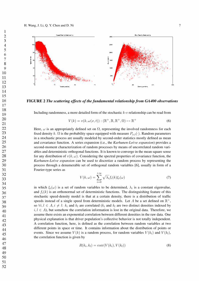
FIGURE 2 The scattering effects of the fundamental relationship from GA400 observations

Including randomness, a more detailed form of the stochastic k-v relationship can be read from

V (k) = v(k, ω(x, t)) : (R+, R, R+,Ω) 7→ R+ (6)

Here, ω is an appropriately defined set on Ω, representing the involved randomness for eachfixed density k. Ω is the probability space equipped with measure Px,t(·). Random parametersin a stochastic process are usually modeled by second-order statistics mostly defined as meanand covariance function. A series expansion (i.e., the Karhunen-Loeve expansion) provides asecond-moment characterization of random processes by means of uncorrelated random vari-ables and deterministic orthogonal functions. It is known to converge in the mean square sensefor any distribution of v(k, ω). Considering the spectral properties of covariance function, theKarhunen-Loeve expansion can be used to discretize a random process by representing theprocess through a denumerable set of orthogonal random variables [6], usually in form of aFourier-type series as

V (k, ω) =+∞∑i=0

√λifi(k)ξi(ω) (7)

in which ξi(ω) is a set of random variables to be determined, λi is a constant eigenvalue,and fi(k) is an orthonormal set of deterministic functions. The distinguishing feature of thisstochastic speed-density model is that at a certain density, there is a distribution of trafficspeeds instead of a single speed from deterministic models. Let A be a set defined on R+,so ∀i, l ∈ A, i 6= l: ki and kl are correlated (ki and kl are two distinct densities indexed byi, l ∈ A), but somehow the correlation information is lost in the original data. Therefore, weassume there exists an exponential correlation between different densities in the raw data. Onephysical explanation is that driver population’s collective behavior is not totally independent.A correlation function, here, is defined as the correlation between random variables at twodifferent points in space or time. It contains information about the distribution of points orevents. Since we assume V (k) is a random process, for random variables V (ki) and V (kl),the correlation function is given by

R(ki, kl) = corr(V (ki), V (kl)) (8)

H. Wang, J. Li, Q. Y. Chen and D. Ni 8

An exponential correlation function is assumed in this paper which is popularly used in varyingdisciplines in the form of

R(ki, kl) = 〈v(ki, ω)v(kl, ω)〉 = σ2 exp(−|ki − kl|α

) (9)

The constants σ2 and α are, respectively, the variance and the correlation length of the process.The correlation length is a measurement of range over which fluctuations in one region of spaceare correlated with those in another region. σ itself is the standard deviation. This process isknown as the Ornstein-Uhlenbeck process. For more information about exponential correlationfunction, interested readers are referred to [34].

Let V (k, ω) be a random function of k defined over domain D, with ω defined on the ran-dom events space Ω. Let V (k) represent the expectation of V (k, ω) over all possible randomprocess realizations. C(ki, kl) is defined as its covariance function with bounded, symmetric,and positive definite properties [6]. It is related to the correlation function by

C(ki, kl) = R(ki, kl)σ(ki)σ(kl) (10)

Following Mercer’s Theorem, by spectral decomposition of covariance function

C(ki, kl) =+∞∑n=0

λnfn(ki)fn(kl) (11)

where λn and fn(k) are, respectively, the eigenvalues and the eigenvectors of the covariancekernel. They can be obtained by solving the homogeneous Fredholm integral equation givenby ∫

DC(ki, kl)fn(k)dki = λnfn(kl) (12)

Equation (12) arises due to the fact that the eigenfunction fi(k) forms a complete orthogonalset satisfying

δij =∫

Dfi(k)fl(k)dk (13)

in which δil is the Kronecker-delta function. Through some algebra, V (k, ω) can be written as

V (k, ω) = V (k) + β(k, ω) (14)

where β(k, ω) is a process with a mean of 0 and a covariance function C(ki, kl). In terms ofthe eigenfunction, fn(k), the process β(k, ω) can be expanded as

β(k, ω) =+∞∑i=0

√λifi(k)ξi(ω) (15)

Thus, the decomposed form of the random process can be written as

V (k, ω) = V (k) + σ(k)+∞∑i=0

fi(k)√

λiξi(ω) (16)

in which, 〈ξi(ω)〉 = 0, 〈ξi(ω)ξl(ω)〉 = δil, and δil =∫D fi(k)fl(k)dk. For practical imple-

mentation, the series is approximated to a finite number by truncating equation (16) at a N th

term, a more specific form of stochastic speed-density relationship can be processed as

V (k, ω) = V (k) + σ(k)N∑

i=0

fi(k)√

λiξi(ω) (17)

H. Wang, J. Li, Q. Y. Chen and D. Ni 9

in which V (k) is the expected speed value of a deterministic speed-density relationship model,and it is open to classic or modified speed-density relationship models. The value of N isgoverned by the accuracy of the eigen-pairs (eigenvalue and eigenfunction) in representing thecovariance function rather than the number of random variables. ξi(ω) are pairwise uncorre-lated random variables. An explicit form of ξi(ω) can be obtained from

ξi(ω) =1√λi

∫D

(V (k, ω)− V (k))fi(k)dk (18)

with mean and covariance function given by

E[ξi(ω)] = 0 (19)

E[ξi(ω)ξl(ω)] = δil (20)

A Gaussian or Beta distribution is assumed for the random variable ξi(ω) through investigationof empirical data. The Beta distribution matches the empirical observations well, but it couldnot guarantee the convergence of the Karhunen-Loeve expansion . Due to the convergenceconcern, a Gaussian distribution is used as it surely guarantees the convergence of Karhunen-Loeve expansion. However, the limitation of Gaussian distribution is that it generates negativespeeds during simulation.

3.2 AlgorithmIn sum, the algorithm to simulate the proposed stochastic speed-density model is devised andcoded as followed,

1. Read empirical speed-density data k and v, the data is sorted by k in a non-decreasingorder k = 1, 2, . . . , kmax (Note: kmax is the maximum observed density at the specificstation).

2. Compute the empirical mean speed V (k) and σ(k), the computed mean and variancecurve is smoothed by smoothing techniques. (Note: It seem self-evident if the simula-tion totally depends on the empirical data and then compares the simulated speed-densitymodel with the empirical observations. To improve model transferability and predictabil-ity, a parameter based deterministic speed-density model is needed to approximate themean. The approximation function of variance comes from the empirical investigationof 78 stations’ variance assuming variance is a function of density. Now, for a new sta-tion (location), the stochastic speed-density model will not require the empirical data,but rather it will need a set of location-based parameters varying with road geometry).

3. Determine a target covariance function C(ki, kl), compute the correlation by the as-sumed exponential correlation function (9) and decompose the covariance function C(ki, kl)into eigenvalues and eigenfunctions using Equation (11).

4. Generate N sample functions of the non-Gaussian process using the truncated K-L ex-pansion: V

(n)N (k, ωi) = V (k) + σ(k)

∑Ni=0 fi(k)

√λiξ

(n)i (ω), i = 1, 2, . . . , N , here

n is iteration number and i is sample number. V (k) and σ(k) is known from step2, λi and fi(k) is given by solving equation (12). The resulting eigenfunctions arefi(k) = cos(θik)√

a+sin(2θia)

2θi

and f∗i (k) = sin(θ∗i k)√a−

sin(2θ∗i

a)

2θ∗i

for even and odd i respectively. The

corresponding eigenvalues are λi = 2cθ2i +c2

and λ∗i = 2cθ∗2i +c2

.

H. Wang, J. Li, Q. Y. Chen and D. Ni 10

5. Pick ki, generate N samples, also generate N samples of identically independent dis-tributed Gaussian random variables ξi(ω)N

i=1. Go to step 4.

6. Pick another kl, repeat step 5 until kmax, stop.

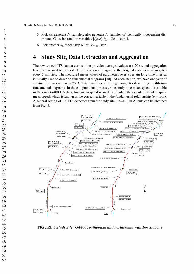
4 Study Site, Data Extraction and AggregationThe raw GA400 ITS data at each station provides averaged values at a 20 second aggregationlevel, when used to generate the fundamental diagrams, the original data were aggregatedevery 5 minutes. The measured mean values of parameters over a certain long time intervalis usually used to describe fundamental diagrams [30]. At each station, we have one-year ofcontinuous observations in 2003. This time interval is long enough for describing equilibriumfundamental diagrams. In the computational process, since only time mean speed is availablein the raw GA400 ITS data, time mean speed is used to calculate the density instead of spacemean speed, which is known as the correct variable in the fundamental relationship (q = kvs).A general setting of 100 ITS detectors from the study site (GA400) in Atlanta can be obtainedfrom Fig. 3.

FIGURE 3 Study Site: GA400 southbound and northbound with 100 Stations

H. Wang, J. Li, Q. Y. Chen and D. Ni 11

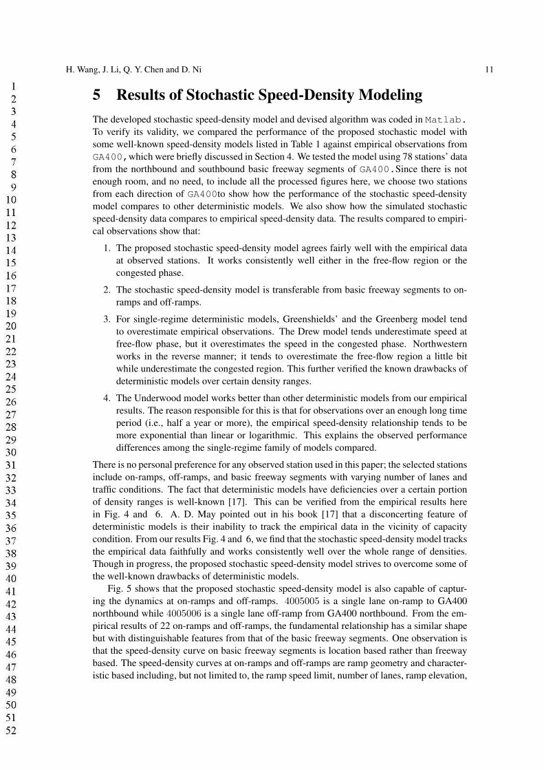
5 Results of Stochastic Speed-Density ModelingThe developed stochastic speed-density model and devised algorithm was coded in Matlab.To verify its validity, we compared the performance of the proposed stochastic model withsome well-known speed-density models listed in Table 1 against empirical observations fromGA400,which were briefly discussed in Section 4. We tested the model using 78 stations’ datafrom the northbound and southbound basic freeway segments of GA400.Since there is notenough room, and no need, to include all the processed figures here, we choose two stationsfrom each direction of GA400to show how the performance of the stochastic speed-densitymodel compares to other deterministic models. We also show how the simulated stochasticspeed-density data compares to empirical speed-density data. The results compared to empiri-cal observations show that:

1. The proposed stochastic speed-density model agrees fairly well with the empirical dataat observed stations. It works consistently well either in the free-flow region or thecongested phase.

2. The stochastic speed-density model is transferable from basic freeway segments to on-ramps and off-ramps.

3. For single-regime deterministic models, Greenshields’ and the Greenberg model tendto overestimate empirical observations. The Drew model tends underestimate speed atfree-flow phase, but it overestimates the speed in the congested phase. Northwesternworks in the reverse manner; it tends to overestimate the free-flow region a little bitwhile underestimate the congested region. This further verified the known drawbacks ofdeterministic models over certain density ranges.

4. The Underwood model works better than other deterministic models from our empiricalresults. The reason responsible for this is that for observations over an enough long timeperiod (i.e., half a year or more), the empirical speed-density relationship tends to bemore exponential than linear or logarithmic. This explains the observed performancedifferences among the single-regime family of models compared.

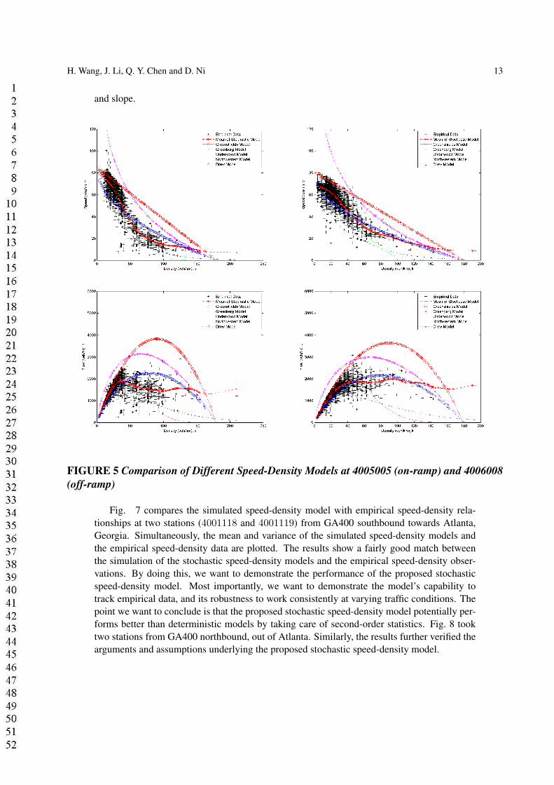
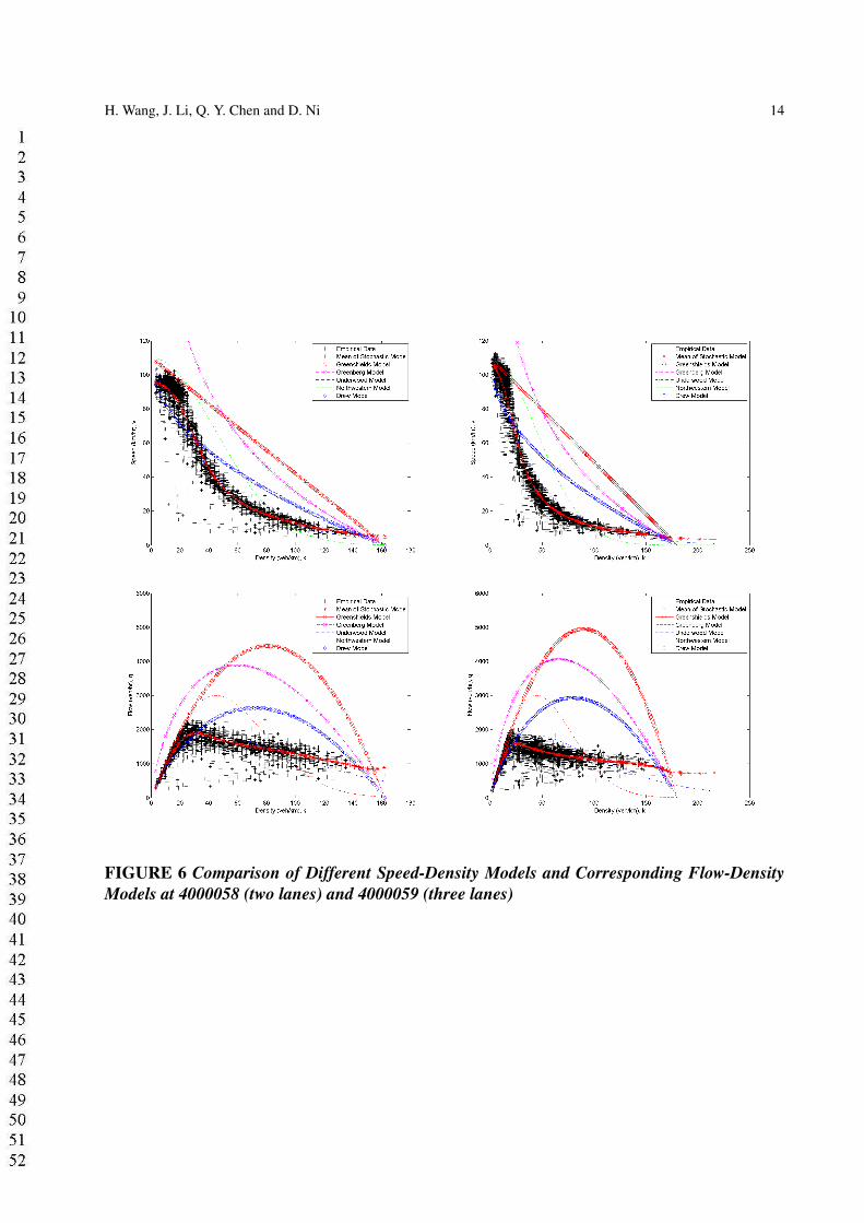
There is no personal preference for any observed station used in this paper; the selected stationsinclude on-ramps, off-ramps, and basic freeway segments with varying number of lanes andtraffic conditions. The fact that deterministic models have deficiencies over a certain portionof density ranges is well-known [17]. This can be verified from the empirical results herein Fig. 4 and 6. A. D. May pointed out in his book [17] that a disconcerting feature ofdeterministic models is their inability to track the empirical data in the vicinity of capacitycondition. From our results Fig. 4 and 6, we find that the stochastic speed-density model tracksthe empirical data faithfully and works consistently well over the whole range of densities.Though in progress, the proposed stochastic speed-density model strives to overcome some ofthe well-known drawbacks of deterministic models.

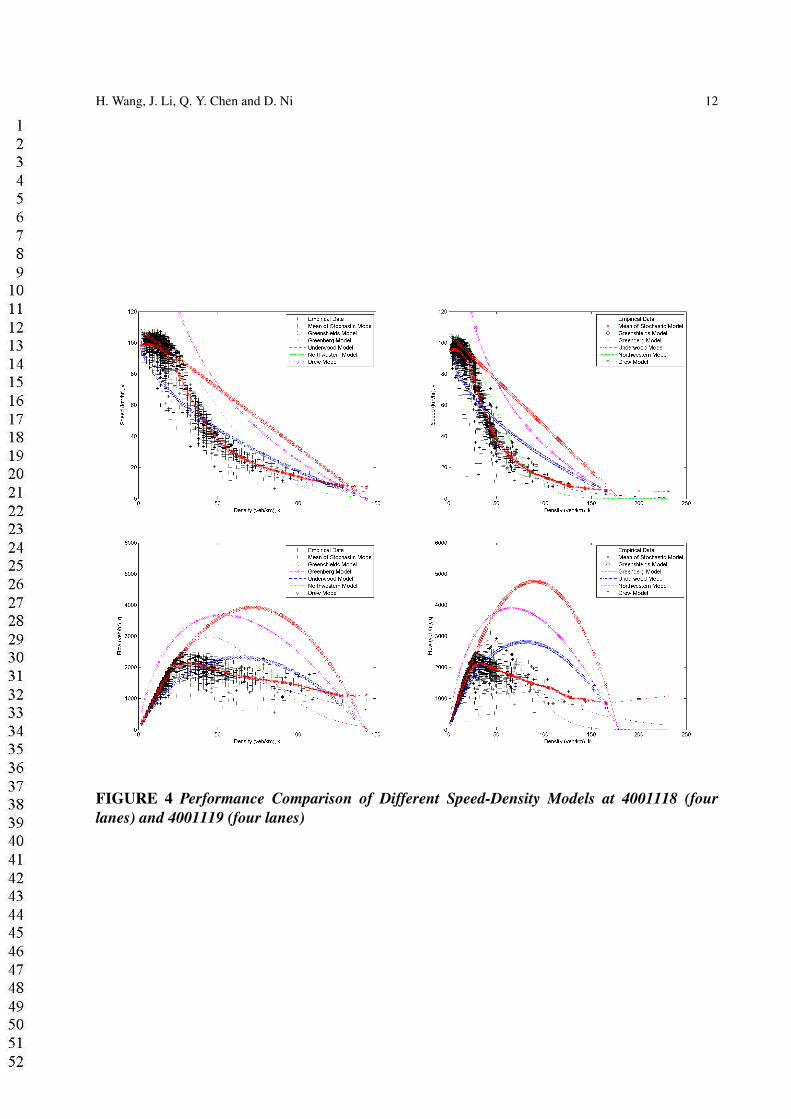
Fig. 5 shows that the proposed stochastic speed-density model is also capable of captur-ing the dynamics at on-ramps and off-ramps. 4005005 is a single lane on-ramp to GA400northbound while 4005006 is a single lane off-ramp from GA400 northbound. From the em-pirical results of 22 on-ramps and off-ramps, the fundamental relationship has a similar shapebut with distinguishable features from that of the basic freeway segments. One observation isthat the speed-density curve on basic freeway segments is location based rather than freewaybased. The speed-density curves at on-ramps and off-ramps are ramp geometry and character-istic based including, but not limited to, the ramp speed limit, number of lanes, ramp elevation,

H. Wang, J. Li, Q. Y. Chen and D. Ni 12

FIGURE 4 Performance Comparison of Different Speed-Density Models at 4001118 (fourlanes) and 4001119 (four lanes)

H. Wang, J. Li, Q. Y. Chen and D. Ni 13

and slope.

FIGURE 5 Comparison of Different Speed-Density Models at 4005005 (on-ramp) and 4006008(off-ramp)

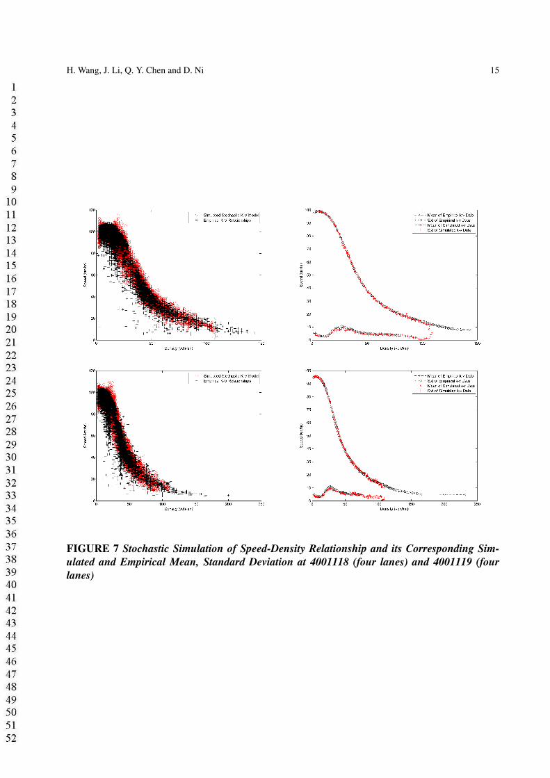
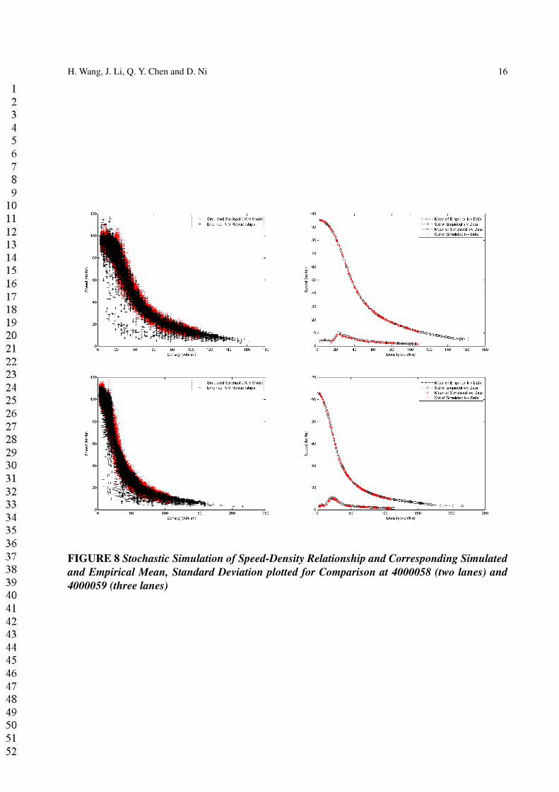
Fig. 7 compares the simulated speed-density model with empirical speed-density rela-tionships at two stations (4001118 and 4001119) from GA400 southbound towards Atlanta,Georgia. Simultaneously, the mean and variance of the simulated speed-density models andthe empirical speed-density data are plotted. The results show a fairly good match betweenthe simulation of the stochastic speed-density models and the empirical speed-density obser-vations. By doing this, we want to demonstrate the performance of the proposed stochasticspeed-density model. Most importantly, we want to demonstrate the model’s capability totrack empirical data, and its robustness to work consistently at varying traffic conditions. Thepoint we want to conclude is that the proposed stochastic speed-density model potentially per-forms better than deterministic models by taking care of second-order statistics. Fig. 8 tooktwo stations from GA400 northbound, out of Atlanta. Similarly, the results further verified thearguments and assumptions underlying the proposed stochastic speed-density model.

H. Wang, J. Li, Q. Y. Chen and D. Ni 14

FIGURE 6 Comparison of Different Speed-Density Models and Corresponding Flow-DensityModels at 4000058 (two lanes) and 4000059 (three lanes)

H. Wang, J. Li, Q. Y. Chen and D. Ni 15

FIGURE 7 Stochastic Simulation of Speed-Density Relationship and its Corresponding Sim-ulated and Empirical Mean, Standard Deviation at 4001118 (four lanes) and 4001119 (fourlanes)

H. Wang, J. Li, Q. Y. Chen and D. Ni 16

FIGURE 8 Stochastic Simulation of Speed-Density Relationship and Corresponding Simulatedand Empirical Mean, Standard Deviation plotted for Comparison at 4000058 (two lanes) and4000059 (three lanes)

H. Wang, J. Li, Q. Y. Chen and D. Ni 17

6 Conclusion and Future WorkThough deterministic speed-density relationship models can explain physical phenomenonsunderlying fundamental diagrams, the stochastic model is more accurate and more suitable todescribe traffic phenomenon. From the results of stochastic model, we find out that a stochasticspeed-density model matches the empirical observations better than deterministic ones. Fol-lowing from this result, the LWR type conservation equation can be revisited in a stochasticsetting of speed-density relationship. The LWR model in a stochastic setting is potentially ca-pable to capture some interesting features (i.e., spontaneous congestion) where deterministicmodels fail. Another benefit from a stochastic speed-density model is its capability to performreal-time on-line prediction while deterministic models are claimed to be insufficient. Futurework could be done to improve the model transferability and predictability. The accuracy andoptimality of the Karhunen-Loeve Expansion algorithm could be improved and tested withother correlation functions to further fine-tune the proposed stochastic speed-density model ascompared to empirical observations.

7 AcknowledgementThe authors thank Steven Andrews for his help with improving the quality and readability ofthis paper.

H. Wang, J. Li, Q. Y. Chen and D. Ni 18

References[1] Jr., S. J. Y. Smith, J. M. Modeling Circulation Systems in Buildings Using State Depen-

dent Queueing Models,Queueing Syst., 1989, 4, pages: 319-338.

[2] Rajat, J. Smith, J. Modeling Vehicular Traffic Flow using M/G/C/C State DependentQueueing Models. Transportation Science, 1997, 31, pages: 324-335.

[3] Gabor S, C. I. The analogies of highway and computer network traffic. Physica A, 2002,307, pages: 516-526.

[4] Helbing, D. Traffic and Related Self-Driven Many-Particle Systems. Rev. Mod. Phys.,2001,73,1067-1141.

[5] Chowdhury, D. Schadschneider, A., Nishinari, K. Physics of Transport and Traffic Phe-nomena in Biology: from molecular motors and cells to organisms. Physics of Life Re-views, 2005, 2, 318.

[6] Roger G. Ghanem, P. D. S. Stochastic Finite Elements: A Spectral Approach. Springer-Verlag, New York, 1990.

[7] Jia Li, Qian-Yong Chen, H. Wang. D. Ni. Investigation of LWR model with flux func-tion driven by random free flow speed. Symposium on The Greenshields FundamentalDiagram: 75 Years Later, 2008.

[8] Gazis, D. C. The Origins of Traffic Theory,Operation Research, INFORMS, 2002, 50,pages: 69-77.

[9] Greenshields, B. D. A Study in Highway Capacity. Highway Research Board Proceed-ings, 1935, 14, pages: 448-477.

[10] Greenberg, H. An analysis of traffic flow. Operation Research, 1959, 7, pages: 79-85.

[11] Underwood, R. T. Speed, Volume, and Density Relationship. Quality and Theory of Traf-fic Flow, Yale Bur. Highway Traffic, New Haven, Connecticut, 1961, pages: 141-188.

[12] J. S. Drake, J. L. Schofer, A. D. May. A Statistical Analysis of Speed Density Hypothe-ses. Third International Symposium on the Theory of Traffic Flow Proceedings, ElsevierNorth Holland, Inc. New York, 1967.

[13] Pipes, L. A. Car-Following Models and the Fundamental Diagram of Road Traffic. Trans-portation Research, 1967, 1, pages: 21-29.

[14] Drew, D. R. Traffic Flow Theory and Control, McGraw-Hill Book Company, 1968, Chap-ter 12.

[15] Douglas I. Rouse. Stochastic Modeling of Plant Disease Epidemic Processes, Handbookof Applied Mycology Sail and Plants, Vol. 1 edited by Dilip K. Arora etc, 1991.

[16] Lu Sun, J. Z. Development of Multiregime Speed-Density Relationship by Cluster Analy-sis. Transportation Research Record, 2005, Volume 1934, pages: 64-71.

[17] May, A. D. Traffic Flow Fundamentals, Prentice Hall, Englewood Cliffs, 1990.

[18] Hall, F.L., Hurdle, V.F., Banks, J.H. A synthesis on recent work on the nature of speed-flow and flow-occupancy (or density) relationships on freeways. Transportation Res. Rec.1365, pp. 12-18, 1992.

[19] James H. Banks. Review of Empirical Research on Congested Freeway Flow. Transporta-tion Res. Rec. 1802, pp. 225-232, 2002.

H. Wang, J. Li, Q. Y. Chen and D. Ni 19

[20] Edie, L. C. Car-Following and Steady-State Theory for Noncongested Traffic. OperationResearch, 1961, 9, pages: 66-76.

[21] Li, M. Z. F. A Generic Characterization of Equilibrium Speed-Flow Curves. Transporta-tion Science, 2008, 42, pp. 220-235.

[22] Lonnie E. Haefner, M. L. Traffic Flow Simulation for an Urban Freeway Corridor, Trans-portation Conference Proceedings, 1998.

[23] Kuhne, R., Rodiger, M. Macroscopic simulation model for freeway traffic with jams andstop-start waves. Simulation Conference, 1991. Proceedings., Winter, 1991, pages: 762-770.

[24] J. M. DEL CASTILLO, F. G. B. On the Functional Form of the Speed-DensityRelationship–I: General Theory. Transportation Research Part B: Methodological, 1995,29B, pages: 373-389.

[25] J. M. DEL CASTILLO, F. G. B. On the Functional Form of the Speed-Density Relationship–II: Empirical Investigation. Transportation Research PartB:Methodological, 1995, 29B, pages: 391-406.

[26] Gazis, D. C. Herman, R., Potts, R. B. Car-Following Theory of Steady-State Traffic Flow.Operations Research, INFORMS, 1959, 7, pages: 499-505.

[27] Gazis, D. C. Herman, R., Rothery, R. W. Nonlinear Follow-The-Leader Models of TrafficFlow. Operations Research, INFORMS, 1961, 9, pages: 545-567.

[28] Tavana H., Mahmassani, H. S. Estimation and application of dynamic speed-density rela-tions by using transfer function models. Transportation Research Record, 2000, pages:47-57.

[29] Xiao Qin, Mahmassani Hani S. Adaptive calibration of dynamic speed-density rela-tions for online network traffic estimation and prediction applications. TransportationResearch Record, 2004, pages: 82-89.

[30] Ning, Wu. A new approach for modeling of Fundamental Diagrams. Transportation Re-search Part A: Policy and Practice, 2002, 36, pages: 867-884.

[31] Daganzo, C. The cell transmission model: a dynamic representation of highway trafficconsistent with the hydrodynamic theory, Transportation Research Part B: Methodologi-cal, 1994, 28, pp. 269-287.

[32] Schreckenberg, M., Schadschneider, A., Nagel, K., Ito, N. Discrete stochastic models fortraffic flow, Physical Review E, 1995, 51, pp. 2939.

[33] Galstyan, A., Lerman, K. A Stochastic Model of Platoon Formation in Traffic Flow, 2001.

[34] Paciorek, C. Nonstationary Gaussian Processes for Regression and Spatial Modelling.Carnegie Mellon University, Pittsburgh, Pennsylvania, 2003.

[35] SOPASAKIS, A., KATSOULAKIS, M. A. Stochastic Modeling and Simulation of trafficFlow: Asymetric Single Exclusion Process with Arrhenius Look-Ahead Dynamics. SIAMJournal on Applied Mathematics, 20060201, 66, pages: 921-944.

[36] Sopasakis, A. Stochastic noise approach to traffic flow modeling. Physica A StatisticalMechanics and its Applications, 2004, 342, 741-754.

[37] Reinhard Mahnke, Christof Liebe, R. K. H. Wang. Traffic Flow Perspectives: From Fun-damental Diagram to Energy Balance. Symposium on The Greenshields FundamentalDiagram: 75 Years Later, 2008.

H. Wang, J. Li, Q. Y. Chen and D. Ni 20

[38] Jou, Yow-Jen, Lo, S. Modeling of Nonlinear Stochastic Dynamic Traffic Flow. Trans-portation Research Record, 2001, pages: 83-88.

[39] Lehoczky, J. P. Stochastic Models in Traffic Flow Theory. Intersection Control HighwayResearch Record, 1970, 3, pages: 1-7.

[40] Bonzani I., M. L. Stochastic modelling of traffic flow. Mathematical and Computer Mod-elling, 2002, 36, pp. 109-119.

[41] Rene Boel, L. M. A compositional stochastic model for real time freeway traffic simula-tion, Transportation Research Part B: Methodological, 2006, 40, pp. 319-334.

[42] Geistefeldt, J. Empirical Relation Between Stochastic Capacities and Capacities Ob-tained From The Speed-Flow Diagram. Symposium on The Greenshields FundamentalDiagram: 75 Years Later, Sponsored by Transportation Research Board, Woods Hole,Massachusetts, 2008.