A 12-week project in

Speech Coding and Recognition

by Vedrana Andersen

vedrana@itu.dk

(130274-xxxx)

and Fu-Tien Hsiao

hsiao@itu.dk

(031278-xxxx)

Project supervisor:

John Aasted Sørensen

IT University of Copenhagen

September – November 2005.

CONTENTS 2

Contents

1 Introduction 3

2 An Introduction to Speech Signals 52.1 Speech Signals in the Time Domain . . . . . . . . . . . . . . . . 52.2 Speech Signals in the Frequency Domain . . . . . . . . . . . . . 112.3 Speech Spectrogram . . . . . . . . . . . . . . . . . . . . . . . . 162.4 Homework . . . . . . . . . . . . . . . . . . . . . . . . . . . . . 19

3 Linear Prediction Analysis 203.1 Short-term Autocorrelation . . . . . . . . . . . . . . . . . . . . . 203.2 Autocorrelation Method for LP Analysis . . . . . . . . . . . . . . 263.3 Levison-Durbin Recursion . . . . . . . . . . . . . . . . . . . . . 283.4 Inverse Filtering Computation . . . . . . . . . . . . . . . . . . . 303.5 Formant Estimation . . . . . . . . . . . . . . . . . . . . . . . . . 323.6 Pitch and Gain Estimation . . . . . . . . . . . . . . . . . . . . . 353.7 Homework . . . . . . . . . . . . . . . . . . . . . . . . . . . . . 38

4 Speech Coding and Synthesis 404.1 Perceptual Weighting Filter . . . . . . . . . . . . . . . . . . . . . 404.2 Excitation Sequence . . . . . . . . . . . . . . . . . . . . . . . . . 424.3 CELP Synthesizer . . . . . . . . . . . . . . . . . . . . . . . . . . 424.4 Quantization . . . . . . . . . . . . . . . . . . . . . . . . . . . . . 454.5 Homework . . . . . . . . . . . . . . . . . . . . . . . . . . . . . 46

5 Speech Recognition 475.1 Feature Extraction . . . . . . . . . . . . . . . . . . . . . . . . . . 475.2 Vector Quantization . . . . . . . . . . . . . . . . . . . . . . . . . 485.3 Training the HMM . . . . . . . . . . . . . . . . . . . . . . . . . 515.4 Recognition using the HMM . . . . . . . . . . . . . . . . . . . . 525.5 Homework . . . . . . . . . . . . . . . . . . . . . . . . . . . . . 56

1 INTRODUCTION 3

1 Introduction

The human sense of hearing and the human’s ability to talk are very importantmeans of communication, which are gaining importance for IT-systems. Therefore,after completing the ‘Signal Processing’ course in our first semester of studies atIT University of Copenhagen, we decided to join the ‘Speech Coding and Recog-nition’ project cluster and to carry out the 12-week project in ‘Speech Coding andRecognition’. The project aims at introducing basic principles and fundamentalmodels for production, perception, coding and recognition of the speech signals.Those models are necessary for the understanding, construction and performanceevaluation of IT-systems, which use speech as one of the input/output media.

We started the work on this project by attending the weekly lessons given byour supervisor, John Aasted Sørensen. First set of lessons covered the models forspeech production, human vocal tract and linear prediction used for parameter esti-mation. After that we moved to speech coding using analysis-by-synthesis method.Lastly we turned to speech recognition using the hidden Markov model.

In parallel with attending the lessons, we worked on the hands-on exercisesusing the speech processing algorithms represented inMATLAB . Finally, towardthe end of the project period we compiled the completed exercises into this projectreport.

There are in total four exercises in the report. The first two exercises are well-documented, stating both the detailed explanation of the considered topic, imple-mentations of neededMATLAB functions, generated plots and our comments. Inthe last two exercises we put focus on our own observations and conclusions. Thereader should keep in mind that this report forms a comprehensive text only to-gether with the exercises. The numbers in the form (x.x.x) are references to theexercise number in the exercise sheets.

First exercise, ‘An Introduction to Speech Signals’, presents the simplifiedmodel for the speech production process, where the speech is described as a se-ries of the steady-state sounds. The difference between modeling voiced and un-voiced sounds is explained. In the time domain, we use short-time power and zeroscrossing measure to determine whether the signal is voiced or unvoiced. In the fre-quency domain we analyze DFT based magnitude spectrum of the speech signals.We determine formants and we estimate pitch period from the harmonic productspectrum. Based on those analyses, we also try to estimate the pitch in a slidingwindow. We observe the speech spectrograms and notice the temporal changes inmagnitude spectra.

In the second exercise, ‘Linear Prediction Analysis’, we first introduce theshort-term autocorrelation. We then assume all-pole model of the speech produc-tion. This model leads us to the autoregressive speech production, where the speechsignal can be predicted using a linear combination of its past values. We use au-tocorrelation method to find the LP coefficients, first by ‘brute force’ and later byLevison-Durbin algorithm. This recursive algorithm utilizes the fact that the auto-correlation matrix is Toeplitz, and that it’s elements are is in a special relationship

1 INTRODUCTION 4

to the elements of the autocorrelation vector. Finally, we perform frame based LPanalysis of the speech signals. We also used different techniques for pitch and gainestimation and use the results to synthesize the signal.

Third exercise, ‘Speech Coding and Synthesis’, considers the problem of repre-senting speech signals digitally in the way appropriate for transmission over com-munication channels. In the coding part (sending end), we apply LP analysis andperceptual weighting. We focus on Code-Excited Linear Prediction coder (CELP)analyze-by-synthesis method, in which the excitation sequence is selected froma Gaussian codebook. We useMATLAB function that performs frame-based es-timation of LP parameters, gain and excitation parameters. In the decoding part(receiving end) we synthesize the signal and discuss the quality of it for differ-ent settings. We also try using quantization of the transmitted parameters, and wediscuss influence of the quantization on the synthesized signal.

In the last exercise, ‘Speech Recognition’, we gradually build a word recog-nizer able to recognize ten words. The word recognizer is based on the hiddenMarkov model (HMM). First we apply the LP analysis to extract feature vectorscontaining cepstral coefficients from the training words. We then perform vectorquantization to produce a codebook, so that each speech signal can be representedas series of symbols. Then we use forward-backward reestimation algorithm totrain each HMM on a given word, by maximizing the probability that the wordwas produced by the HMM. Finally, we can use built models to recognize new,unknown words by finding the HMM with the highest probability of producing theword. We analyzed each of those steps, and performed the tests on the word recog-nizer changing the block size and spacing, the LPC and cepstrum order, and thecodebook size.

Through this project we gained the theoretical insight of the covered topics andof algorithms used in speech processing. We also obtained the practical experienceon implementing and using simple speech processing tools which can serve asbuilding blocks for more advanced applications.

We would like to thank our supervisor, John Aasted Sørensen, for his guidanceduring the lessons, and valuable comments and suggestions for carrying out theexercises and writing the project report.

2 AN INTRODUCTION TO SPEECH SIGNALS 5

2 An Introduction to Speech Signals

2.1 Speech Signals in the Time Domain

In technical discussions, the entire combination of all speech production cavitiesis referred to as the vocal tract and comprises the main acoustic filter. The filter isexcited by organs below it (vocal cords, lungs, etc.) and loaded at its main outputby a radiation impedance due to the lips.

(1.4.1) figure 1 represents an amplitude waveform of the speech signal ‘She hadyour dark suit in greasy wash water all year’. From the figure we can see that thespeech is a series of steady-state segments with intermediate transitions. Locallystationary speech segments (or frames) are denoted short-time descriptions.

0 1 2 3 4 5

x 104

−1

−0.8

−0.6

−0.4

−0.2

0

0.2

0.4

0.6

0.8

1

time index

ampl

itude

Figure 1: Amplitude waveform of the speech signal ‘She had your dark suit in greasy washwater all year’ uttered by an adult male (3.5 seconds at 16 kHz).

Depending on the manner of excitation, speech segments can be divided intovoiced and unvoiced speech sounds. A voiced speech sound is generated froma quasi-periodic vocal-cord sound with a fundamental frequency or pitch usuallyfound to be below a few hundred Hertz. An unvoiced speech sound is generatedfrom a random sound produced by turbulent airflow.

(1.4.2) On the figure 2 we have plots of two frames, one representing the voicedsound /a/ in ‘dark’, and the other representing unvoiced sound /S/ in ‘wash’. Let’slook closer at the some characteristics of the two types of excitation.

(1.4.3) As expected, we observe clear periodicity in the voiced sound, with thefundamental period of around 130 samples. There is no obvious periodicity in theunvoiced sound—it looks random.

The amplitudes of the voiced sounds are approximately 10 times higher than

2 AN INTRODUCTION TO SPEECH SIGNALS 6

1.45 1.455 1.46 1.465 1.47 1.475 1.48 1.485 1.49

x 104

−1

−0.5

0

0.5

1

time index

ampl

itude

3.55 3.555 3.56 3.565 3.57 3.575 3.58 3.585 3.59

x 104

−0.1

−0.05

0

0.05

0.1

time index

ampl

itude

Figure 2: Plots of the two speech frames of 400 samples (25 ms) from the speech signalplotted at figure 1. Top: /a/ in ‘dark’ (sample numbers 14501–14900), bottom: /S/ in‘wash’ (sample numbers 35501–35900).

those of the unvoiced sound. In other words, the average power of voiced soundsis much higher than the average power of the unvoiced sounds.

The number of zero crossings is much larger for the unvoiced sound than for thevoiced sound. In this particular case of voiced sound we have 12 zero crossings inone period. In the same time frame, the number of zero crossings for the unvoicedsound is well above 40.

(1.4.4) For time-variant signalx(n), the short-time powerPx(m) can be mea-sured for theN-length frame ending at timem, i.e.,

Px(m) =1N

m

∑n=m−N+1

|x(n)|2

Each time the window is shifted one sample, the powerPx could be recalculated,however, it is easier to update the previous value ofPx as

Px(m) = Px(m−1)+1N

(|x(m)|2−|x(m−N)|2)

TheMATLAB functionstpower.m calculates the short-time power of a signal us-ing a sliding window.

function Px = stpower(x,N)

M = length(x);

Px = zeros(M,1);

Px(1:N) = x(1:N)’*x(1:N)/N;

2 AN INTRODUCTION TO SPEECH SIGNALS 7

for (m=(N+1):M)

Px(m) = Px(m-1) + (x(m)^2 - x(m-N)^2)/N;

end

(1.4.5) A short-time zero crossing measure for theN-length interval ending at timem is

Zx(m) =1N

m

∑n=m−N+1

|signx(n)−signx(n−1)|2

The MATLAB function stzerocross.m implementsZx(m) using a sliding win-dow.

function Zx = stzerocross(x,N)

M = length(x);

Zx = zeros(M,1);

Zx(1:N+1) = sum(abs(sign(x(2:N+1)) - sign(x(1:N))))/(2*N);

for (m=(N+2):M)

Zx(m) = Zx(m-1) + (abs(sign(x(m)) - sign(x(m-1))) ...

- abs(sign(x(m-N)) - sign(x(m-N-1))))/(2*N);

end

(1.4.6) We used short-time power and short-time zero crossing measure to analyzethe utterance ‘four’.

load digits;

N = 300;

x = digits.four1;

Px = stpower_r(x,N);

Zx = stzerocross_r(x,N);

plot([Px*1e-5 Zx x/2000])

On the figure 3 we have the plot of the speech signal ‘four’, together with the short-time power and zero crossing measure. From the plot of the speech signal we caneasily see that the utterance ‘four’ consists of the unvoiced part /f/ and the voicedpart /o/ . We can see that the short-time power of the unvoiced part is close to zero,while for the voiced part it reaches 10 000 times larger values. The short-time zerocrossing measure shows opposite behavior, but the differences between voiced andunvoiced part are not so drastic in this case. The unvoiced part of the utterance hasthe short-time zero crossing measure that is approximately five times larger thanthe short-time zero crossing measure for the voiced part.

Short-time power and zero crossing measure can be used for initial voiced/un-voiced segmentation. For a given speech signal, short-time power and zero crossingmeasure can be calculated using the sliding window of a certain length. The mid-dle sample in the window can be labeled voiced if the short-time power is above acertain threshold and the short-time zero crossing measure below certain threshold.Power thresholds can be expressed relative to maximal values of short-time power.

2 AN INTRODUCTION TO SPEECH SIGNALS 8

0 1000 2000 3000 4000 5000 6000−0.4

−0.2

0

0.2

0.4

0.6

0.8

1

time index

ampl

itude

/ 20

00, s

tpow

er /

105 , s

tzer

ocro

ss

Figure 3: Scaled amplitude waveform of the utterance ‘four’ (green), together with thescaled short-time power (blue) and zero crossing measure (red) obtained using the slidingwindow of 300 samples (30 ms at 10 kHz).

0 1000 2000 3000 4000 5000

−1

−0.8

−0.6

−0.4

−0.2

0

0.2

0.4

0.6

0.8

1

time index

ampl

itude

/ 50

0, s

egm

enta

tion

Figure 4: Amplitude waveform of the speech signal ‘four’ (green), and the initial voiced/u-vioced segmentation (blue). Segmentation is based on short-time power and zero crossingmeasure as on the figure 3. Thresholds used were 0.1 for short-time power, and 0.3 forshort-time zero crossing measure.

2 AN INTRODUCTION TO SPEECH SIGNALS 9

MATLAB functionvoiunvoi.m implements this segmentation.

function voi = voiunvoi(x,N,Pth,Zth)

Px = stpower(x,N);

Zx = stzerocross(x,N);

voi = (Px>Pth*max(Px)) & (Zx<Zth);

voi = [voi(fix(N/2)+1:length(voi));voi(length(voi))*ones(fix(N/2),1)];

The results of using functionvoiunvoi on the speech signal ‘four’ are shown onfigure 4.

Sx=voiunvoi(x,300,0.1,0.3);

plot([Sx, x/800])

The classical discrete-time model for the speech production process assumes thatthe sound-generating excitation is linearly separable from the vocal tract filter. Thevocal tract changes shape relatively slowly with time, and thus it can be modeledas a slowly time-varying filter which imposes its frequency-response properties onthe spectrum of the excitation.

A voiced speech sound can be modeled by a sequence of impulses, which arespaced by a fundamental period equal to the pitch period. This signal then excitesa linear filter whose impulse response equals the vocal-cord sound pulse.

An unvoiced speech sound is generated from an excitation which consists sim-ply of a white noise source.

(1.4.7) Looking at the two speech frames we analyzed in the task (1.4.2), fig-ure 2, it is not difficult to recognize elements from this model. Voiced sound canbe modeled by the filtered impulse train, and the unvoiced sound can be modeledby filtered white noise.

(1.4.8) On figure 5 we have plots of four vowels in frames of 300 samples (30ms at 10 kHz) and we’ll try to estimate the pitch period for each utterance. Bylooking at the plot of the speech signal we can conclude that for all four plots thereis almost the same distance between two neighboring pitch peaks, so the pitchperiod is almost the same for each vowel. Let’s estimate it.

The distance between two neighboring pitch peaks is approximately 90 sam-ples, so we haveTp = 90. We know the sampling frequencyFs = 10 kHz, so wehave

Tp =tp

Fs=

9010 kHz

= 9 ms

Fp = fp ·Fs =Fs

tp=

10 kHz90

≈ 111 Hz

The pitch period is 9 ms, and the pitch frequency 111 Hz. We can also concludethat the speaker is a man, since the pitch frequency of 111 Hz falls into the rangetypical for men. This is confirmed by listening to the speech signal.

2 AN INTRODUCTION TO SPEECH SIGNALS 10

0 100 200 300−1500

−1000

−500

0

500

1000

time index

ampl

itude

0 100 200 300−1000

−500

0

500

1000

time index

ampl

itude

0 100 200 300−2000

−1500

−1000

−500

0

500

1000

1500

time index

ampl

itude

0 100 200 300−1500

−1000

−500

0

500

1000

time index

ampl

itude

Figure 5: Plots of the four vowels in frames of 300 samples (30 ms at 10 kHz). Top left:/a/, top right: /i/, bottom left: /o/, bottom right: /u/.

0 100 200 300−1500

−1000

−500

0

500

1000

1500

time index

ampl

itude

0 100 200 300−2000

−1500

−1000

−500

0

500

1000

time index

ampl

itude

0 100 200 300−1000

−500

0

500

1000

time index

ampl

itude

Figure 6: Plots of the three vowels in frames of 300 samples (30 ms at 10 kHz). Thoseplots should be compared with plots on figure 5.

2 AN INTRODUCTION TO SPEECH SIGNALS 11

(1.4.9) On the figure 6 we see the plots of another three vowels. We can try todetermine which vowels those plots likely represent by comparing the plots on thefigure 6 with the plots on the figure 5. We can see that the top left plot is similar tothe plot of vowel /u/, top right plot is similar to the plot of vowel /a/, and the bottomleft plot is similar to the plot of vowel /i/, so we guessed that the plots representvowels /u/, /a/ and /i/. By listening to the speech signals we could verify that ourguess was correct.

2.2 Speech Signals in the Frequency Domain

The Fourier transformX(ω) is a continuous function of frequency, so in the digitaldomain the sampled spectrum is used to represent an aperiodic signalx(n) of lengthL, which leads to the discrete Fourier transform (DFT) pair

x(n) =1N

N−1

∑k=0

X(k)ej2πkn/N ↔ X(k) =N−1

∑n=0

x(n)e− j2πkn/N

If L≤ N it is possible to recoverx(n) without time-domain aliasing.Limiting the duration of a sequencex(n) to L samples can be done by multi-

plying x(n) by a window functionw(n) of lengthL. According to the windowingtheorem (PM [3], page 302) we have

x(n) = x(n)w(n) ↔ X(ω) =1

2π

∫ π

−πX(θ)W(ω−θ)dθ

The effect of windowing is that energy originating at a single frequency leaks outin the entire frequency range due to the sidelobes ofW(ω), and that the spectralresolution is reduced due to the main lobe width ofW(ω).

(1.5.1) When choosing the window lengthL to analyze speech signals we havecertain limitations. Speech signals are short-time stationary, so the window shouldbe short enough to capture just the steady-state sound. On the other hand, if thewindow is too short, the unwanted effects of windowing are going to dominate thefrequency representation of the speech signal. So, choosing the window length, weneed to consider the tradeoff between time resolution and frequency resolution.

(1.5.2) At figure 7 we have plotted one frame of the speech signal ‘The priceshave gone up enormously in spite of the technological advances’ correspondingto the voiced /Y/ sound in ‘prices’, together with the magnitude spectrum of thesame frame. Since typical speech communication is limited to a bandwidth of 7–8kHz, used speech signal has been low-pass filtered (3.5 kHz) before sampling. Itis evident from the plot of magnitude spectrum that the magnitudes are decreasingfor frequencies towards the end of the frequency range.

(1.5.3) In the simplified model for the speech production process, the vocaltract filter models the entire combination of all speech production cavities. Avoiced speech sound is then modeled by a sequence of impulses (spaced by afundamental period equal to pitch period) which excites a vocal tract filter. The

2 AN INTRODUCTION TO SPEECH SIGNALS 12

frequency response of the vocal tract filterH(z) determines the short-time spectralenvelope of the speech signal. We can verify this by comparing the magnitudespectrum|H(ω)| for the voiced sound with the DFT based magnitude spectrum ofthe voiced sound—one could say that|H(ω)| is obtained by connecting the peakfrequencies of DFT spectrum.

(1.5.4)H(z) can be described by an 8–12 order all-pole filter, i.e., 4–6 resonantfrequencies (formants) usually denotedF1, F2, . . . We can try to determine the for-mants from the DFT based magnitude spectrum. To do that we need to locate 4–6highest peeks of the DFT magnitude spectrum, find their coefficientsk, and thendetermine which frequencies they represent by calculating

f =kN

, F = f ·Fs

We need to use the number of points at which the DFT is evaluatedN = 1024, andthe sampling frequencyFs = 8 kHz. By looking at figure 7 we found

k1 = 78 ⇒ f1 = 781024 = 0.7617 ⇒ F1 = 78

10248 kHz= 609 Hzk2 = 158 ⇒ f2 = 158

1024 = 0.1543 ⇒ F2 = 15810248 kHz= 1234 Hz

k3 = 278 ⇒ f3 = 2781024 = 0.2715 ⇒ F3 = 278

10248 kHz= 2172 Hzk4 = 395 ⇒ f4 = 395

1024 = 0.3857 ⇒ F4 = 39510248 kHz= 3086 Hz

(1.5.5) The excitation of the vocal tract filter is not a single unit pulse but a pe-riodic repetition of pulses (pulse train), so the frequency representation of a voicedspeech sound is a Fourier series. Ideally we should be able to represent a voicedspeech sound by magnitudes of fundamental frequency and its harmonics. Themagnitude spectrum of a voiced sound would in that case be a number of equallyspaced spikes, where the spike closest to 0 represents fundamental frequency. Dueto windowing, we don’t have such a ideal spectrum, but we can still see that a mag-nitude spectrum of a voiced sound is represented by a number of equally spacedpeaks (lobes), where the peak closest to 0 represents pitch.

0 100 200 300−0.6

−0.4

−0.2

0

0.2

0.4

0.6

0.8

sample number

ampl

itude

0 100 200 300 400 500

−60

−40

−20

0

20

frequency / (8kHz/1024)

mag

nitu

de /

dB

Figure 7: Voiced speech frame (37.5 ms at 8 kHz) corresponding to the /Y/ sound in‘prices’. Left: Amplitude waveform, right: magnitude spectrum evaluated at 1024 points.

2 AN INTRODUCTION TO SPEECH SIGNALS 13

Let’s try to estimate the pitch frequency from the spectrum. We need to locatethe peak closest to 0, find it’s coefficient and determine which frequency it repre-sents, using the same method as in the previous task. By looking at the figure 7 wefound

k0 = 20

F0 = f0 ·Fs =k0

NFs =

201024

8 kHz= 156 Hz

(1.5.6) Frequency representation of a voiced speech sound is a Fourier series.However, the DFT based magnitude spectrum of the voiced sound is be influencedby the spectral characteristics of the window functionw(n). The energy originatingat a single frequency leaks out in the entire frequency range due to the sidelobes ofW(ω), and the spectral resolution is reduced due to the width of the main lobe ofW(ω). So the magnitude spectrum of a voiced sound does not have a number ofequally spaced spikes, but a number of equally spaced lobes, where the width ofthe lobes is determined by the width of the main lobe ofW(ω).

We can try to estimate the main lobe width by looking at the figure 7. Wesee that the lobes of the DFT based magnitude spectrum of the voiced sound spanacross the range of 20 coefficientsk. We can express it in terms of normalizedfrequency using the same method as in the previous two tasks

f =kN

=20

1024= 0.0195

So we can estimate the width of the main lobe of theW(ω) to be 0.02 in terms ofnormalized frequency.

(1.5.7) If the DFT is computed with sufficient spectral resolution, then the har-monics of the pitch frequency will be apparent in the spectrum. Thus, the harmonicproduct spectrum defined as

HPSx(ω) =R

∏r=1

X(rω)

can be used to estimate the pitch for some smallR, typically five. TheMATLAB

functionhpspectrum.m implementsHPSx(ω).

function HPSx = hpspectrum(x,N,R)

K = ceil(N/(2*R));

k = 1:K;

X = fft(x.*hann(length(x)),N);

HPSx = X(k);

for (r=2:R)

HPSx = HPSx.*X(r*k-r+1);

end

2 AN INTRODUCTION TO SPEECH SIGNALS 14

0 10 20 30 40 50 60 70 80 90 100

−150

−100

−50

0

50

frequency / (8kHz/1024)

hpsp

ectr

um /

dB

Figure 8: Harmonic product spectrum of the voiced speech frame from the figure 7. WeusedR= 5 andN = 1024to obtain the harmonic product spectrum.

We appliedMATLAB functionhpspectrum.m to the voiced speech frame at fig-ure 7. The harmonic product spectrum of the speech frame is shown at the figure 8.We can use the harmonic product spectrum to estimate the pitch by locating themaximal value of harmonic product spectrum and determining which frequency itrepresents. By looking at the figure 8 we found

k0 = 21

F0 = f0 ·Fs =k0

NFs =

211024

8 kHz= 164 Hz

This result varies a bit from the result obtained in the exercise (1.5.5).(1.5.8) On the figure 9 we have magnitude spectra of the vowels /i/ as in ‘tree’

and /u/ as in ‘boot’. For each of those spectra we can do the same analysis as forthe spectrum on the figure 7, i.e. we can try to determine formants, we can tryto estimate pitch period, and we can look at the effects of windowing in the DFTbased spectra.

(1.5.9) For unvoiced frames (stochastic signal), the DFT should be viewed as astep toward computing a short-time power density spectrum

Γx(ω) = E{X(ω)X(ω)∗}

The phase spectrum is not meaningful in the stochastic case.On the figure 10 we have plotted one frame of the speech signal ‘The prices

have gone up enormously in spite of the technological advances’ corresponding tothe unvoiced /s/ sound in ‘spite’, together with the magnitude spectrum of the sameframe. One should note very small magnitudes of this spectrum.

2 AN INTRODUCTION TO SPEECH SIGNALS 15

0 100 200 300 400 5000

20

40

60

80

100

frequency / (10kHz/1024)

mag

nitu

de /

dB

0 100 200 300 400 5000

20

40

60

80

100

frequency / (10kHz/1024)

mag

nitu

de /

dB

Figure 9: Magnitude spectra of two vowels. Both speech frames had the length of 300samples, and the magnitude spectra was evaluated at 1024 points. Left: /i/ as in ‘tree’,right: /u/ as in ‘boot’.

0 50 100 150

−10

−5

0

5

x 10−3

sample number

ampl

itude

0 100 200 300 400 500

−70

−60

−50

−40

−30

frequency / (8kHz/1024)

mag

nitu

de /

dB

Figure 10: Unvoiced speech frame (20 ms at 8 kHz) corresponding to the /s/ sound in‘spite’. Left: Amplitude waveform, right: magnitude spectrum evaluated at 1024 points.

2 AN INTRODUCTION TO SPEECH SIGNALS 16

2.3 Speech Spectrogram

(1.6.1) On the figure 11 we have an amplitude waveform of the speech signal ‘Shehad your dark suit in greasy wash water all year’, together with the spectrogram ofthe same speech signal.

We can see that the formants structure changes relatively slowly in some timeintervals, but those intervals are separated with shorter or longer transitions wherethe formant structure is not evident. The intervals where formant structure is evi-dent and changing slowly correspond to the voiced parts of the sentence, while thetransitions correspond to unvoiced parts.

(1.6.2) On the figure 12 we have an amplitude waveform of the sound /i/ glis-sandos, together with the spectrogram of the same sound. Glissandos (or pitchsweeps) is a musical term that refers to sliding from one pitch to another, producedfor example by sliding the finger along a keyboard.

Comparing the spectrogram on the figure 12 with the magnitude spectrum of avoiced sound /i/ on the figure 9, it is possible to recognize the formant spectrum forthe /i/ sound—very high magnitudes for very low frequencies (up to 0.5 kHz), fol-lowed by a short range of frequencies with small magnitudes (1–1.5 kHz), followedagain by a longer range of frequencies with high magnitudes (2–3.5 kHz).

Looking at the spectrogram on the figure 12 it is easy to notice the shift inthe pitch frequency. Pitch frequency is represented by the lowest slanted line inthe spectrogram (also the line with highest magnitudes) and the shift in the pitchcorresponds to the slope of the line. The shift in pitch frequency is reflected in allthe harmonics, resulting in spectrogram composed of slanted lines.

(1.6.3)MATLAB functionstpitch.m estimates the short-time pitch in a slidingwindow of lengthN, but only for voiced parts of the speech signal. The functionis based on the voiced/unvoiced segmentationvoiunvoi.m (1.4.6) and the har-monic product spectrumhpspectrum.m (1.5.7). If a frame is voiced, the pitch isestimated using maximal value of harmonic product spectrum for that frame.

function Fp = stpitch(x,N,Pth,Zth,NFFT,R,Fs)

M = length(x);

Fp = zeros(M,1);

voi = voiunvoi(x,N,Pth,Zth);

for (m=N:fix(N/2):M)

n = m-N+1:m;

if all(voi(n))

HPS = abs(hpspectrum(x(n),NFFT,R));

k = find(HPS==max(HPS));

Fp(n) = k;

end

end

wsave = warning; warning(’off’);

Fp = (Fp*Fs/NFFT).*(Fp./Fp);

warning(wsave);

2 AN INTRODUCTION TO SPEECH SIGNALS 17

0 1 2 3 4 5

x 104

−0.5

0

0.5

1

sample number

ampl

itude

Time

Fre

quen

cy

0 0.5 1 1.5 2 2.5 30

2000

4000

6000

8000

Figure 11: Speech signal ‘She had your dark suit in greasy wash water all year’. Top:amplitude waveform, bottom: spectrogram. Magnitude spectrum was calculated in framesof 256 samples, and DFT was evaluated at 256 points.

0 0.5 1 1.5 2 2.5 3 3.5 4 4.5

x 104

−1500

−1000

−500

0

500

1000

sample number

ampl

itude

Time

Fre

quen

cy

0 0.5 1 1.5 2 2.5 3 3.5 40

1000

2000

3000

4000

5000

Figure 12: Voiced sound /i/ glissandos. Top: amplitude waveform, bottom: spectrogram.Magnitude spectrum was calculated in frames of 256 samples, and DFT was evaluated at256 points.

2 AN INTRODUCTION TO SPEECH SIGNALS 18

(1.6.4) We applied functionstpitch.m to two speech signals: the sentence ‘Shehad your dark suit in greasy wash water all year’ uttered by an adult male and thesame sentence repeated by an adult female.

load timit1;

load timit2;

N = 300;

Pth = 0.01;

Zth = 0.3;

NFFT = 1024;

R = 5;

Fs = 16000;

pt1=stpitch_r(timit1,N,Pth,Zth,NFFT,R,Fs);

pt2=stpitch_r(timit2,N,Pth,Zth,NFFT,R,Fs);

plot(pt1)

plot(pt2)

Figure 13 contains amplitude waveforms of the speech signals, and the pitch esti-mations obtained using the functionstpitch.m.

The pitch range for men is usually between 50–250 Hz, while for women therange falls in the interval 120–150 Hz. The results of our pitch estimation fallroughly into these ranges. The pitch estimated from sentence uttered by a womanreached higher values and is generally higher. There is a certain pitch variation inboth sentences, and the pitch variation is larger in the sentence uttered by a woman.

0 1 2 3 4 5

x 104

−0.5

0

0.5

1

sample number

ampl

itude

0 1 2 3 4 5

x 104

−0.5

0

0.5

1

sample number

ampl

itude

0 1 2 3 4 5

x 104

0

200

400

600

800

sample number

pitc

h fr

eque

ncy

/ Hz

0 1 2 3 4 5

x 104

0

200

400

600

800

sample number

pitc

h fr

eque

ncy

/ Hz

Figure 13: Speech signal ‘She had your dark suit in greasy wash water all year’. Left:uttered by an adult male, right: uttered by an adult female, top: amplitude waveform,bottom: pitch estimation using the functionstpitch.

2 AN INTRODUCTION TO SPEECH SIGNALS 19

2.4 Homework

(1.7) In the above exercises, a number of important features has been extractedfrom frames of speech as these frames move through time. These features areeither related to the excitation signals or the vocal-tract. The features that could beused in speech recognition are the features related to the vocal-tract, for examplethe formants of the magnitude spectrum. The discrete Fourier transform could beused to extract/characterize those features.

3 LINEAR PREDICTION ANALYSIS 20

3 Linear Prediction Analysis

3.1 Short-term Autocorrelation

The (long-term) autocorrelation of a power signalx(n) is defined as

rx(η) = limM→∞

12M +1

M

∑n=−M

x(n)x(n−η)

where the indexη is the time shift or lag parameter. In practice, we are dealing withfinite-duration sequencesx(m−N+1),x(m−N+2), . . . ,x(m), and the short-termautocorrelation estimate for the N points ending atmmay be defined as

rx(η ;m) =1

N−η

m

∑n=m−N+1+η

x(n)x(n−η), 0≤ η ≤ N−1

where the autocorrelation sequence for negative lags can be obtained from the re-lation rx(−η) = rx(η). Autocorrelation function estimates as given by the abovementioned formula can be obtained by using theMATLAB function

[r,eta] = xcorr(x,eta_max,’unbiased’)wherex is the signal vector,r is the autocorrelation vector, andeta is a vector oflag indices in the range from-eta_max to eta_max.

(2.1.1) The autocorrelation function for a sinusoidx(n) = Asin(2π f n+ φ) isgiven by

rx(η) =A2

2cos(2π f η), Px = rx(0) =

A2

2We usedMATLAB to verify this result for a sinusoidal signal with normalized fre-quencyf = 0.01, by using the followingMATLAB commands

x = 3*sin(2*pi*0.01*(0:499)’+10);

[r,eta] = xcorr(x,100,’unbiased’);

plot(0:499,x)

plot(eta,r)

On the figure 14 we have a plot of a sinusoidal signalx(n) = 3sin(2π ·0.01+10),together with the autocorrelation of the signal. We can see that the autocorrelationis periodic with the periodN = 100, and the same applies to the sinusoidal signalbecauseN = 1

f = 10.01 = 100. We can also see thatrx(0) = 4.5 which is the average

power of the sinusoidal signalPx = A2

2 = 32

2 = 4.5.(2.1.2) The autocorrelation function for white noise (with variance 1) is given

byrw(η) = δ (η), Pw = rw(0) = 1

We usedMATLAB to verify this result for a noise generated by theMATLAB func-

3 LINEAR PREDICTION ANALYSIS 21

0 50 100 150 200 250 300 350 400 450 500−3

−2

−1

0

1

2

3

sample number

ampl

itude

−100 −80 −60 −40 −20 0 20 40 60 80 100−5

0

5

time shift

auto

corr

elat

ion

Figure 14: The sinusoidal signalx(n) = 3sin(2π ·0.01+10), 0≤ n≤ 499. Top: amplitudewaveform, bottom: short-term autocorrelation over the range[−100,100].

0 50 100 150 200 250 300 350 400 450 500−3

−2

−1

0

1

2

3

sample number

ampl

itude

−100 −80 −60 −40 −20 0 20 40 60 80 100−0.2

0

0.2

0.4

0.6

0.8

1

time shift

auto

corr

elat

ion

Figure 15: The white noise with mean zero and variance one. Top: amplitude waveform,bottom: short-term autocorrelation over the range[−100,100].

3 LINEAR PREDICTION ANALYSIS 22

−100 −80 −60 −40 −20 0 20 40 60 80 100−0.4

−0.2

0

0.2

0.4

0.6

0.8

1

sample number

ampl

itude

−100 −80 −60 −40 −20 0 20 40 60 80 100−0.2

0

0.2

0.4

0.6

0.8

1

1.2

sample number

ampl

itude

Figure 16: Autocorrelation of two white noise signals with different lengths. Top: signallength 200 samples, bottom: signal length 1000 samples.

0 50 100 150 200 250 300 350 400 450 500−4

−2

0

2

4

sample number

ampl

itude

−100 −80 −60 −40 −20 0 20 40 60 80 100−0.5

0

0.5

1

1.5

time shift

auto

corr

elat

ion

Figure 17: The sinusoidal signalx(n) = 0.8 · sin(2π ·0.01+10) corrupted with the whitenoise with mean zero and variance one. Top: amplitude waveform, bottom: short-termautocorrelation over the range[−100,100].

3 LINEAR PREDICTION ANALYSIS 23

tion randn by using the followingMATLAB commands.

w = randn(500,1);

[r,eta] = xcorr(w,100,’unbiased’);

plot(w)

plot(eta,r)

On the figure 15 we have a plot of a random noise, together with the autocorre-lation of the noise. We can see the large peak atrw(0) ≈ 1, while the rest of theautocorrelation is very small.

The accuracy of the estimated autocorrelation function depends on the signallength—estimation is more accurate for the longer signals (larger average interval).To verify this, on the figure 16 we plotted the autocorrelation of two signals withdifferent lengths by using the following commands

w1=randn(200,1);

[r1,eta]=xcorr(w1,100,’unbiased’);

w2=randn(1000,1);

[r2,eta]=xcorr(w2,100,’unbiased’);

plot(eta,r1)

plot(eta,r2)

(2.1.3) Now we added the white noise (with variance one) to the sinusoidal signalx(n) = 0.8·sin(2π ·0.01+10) with normalized frequencyf = 0.01. The observedsignal isy(n) = x(n)+w(n).

x = 0.8*sin(2*pi*0.01*(0:499)’+10);

w = randn(500,1);

y=x+w;

[r,eta] = xcorr(y,100,’unbiased’);

plot(y)

plot(eta,r)

On the figure 17 we have a plot of the observed signal, together with the autocor-relation of the noise. We can see the large peak atry(0) which is the contributionof the random noise, but it is still possible to determine the period of the sinusoidalsignal from the autocorrelation. If we ignore the peak atry(0) and ’smooth’ therest, we can still see that the autocorrelation is periodic with the periodN = 100,which is also the period of the sinusoidal signal.

(2.1.4) We can use the short-term autocorrelation on the speech signal. On thefigure 18 we have a amplitude waveform of the utterance ‘three’. We have cho-sen two 256 point windows from this speech signal: the first window correspondsto the voiced phoneme /i/, and the second window contains an unvoiced regioncorresponding to sound /T/.

load digits;

x = digits.three1;

m = 2756;

3 LINEAR PREDICTION ANALYSIS 24

N = 256;

n = m-N+1:m;

[r,eta] = xcorr(x(n),250,’unbiased’);

plot(1:256, x(n))

plot(eta,r)

m = 500;

N = 256;

n = m-N+1:m;

[r,eta] = xcorr(x(n),250,’unbiased’);

plot(1:256, x(n))

plot(eta,r)

Figure 19 shows the amplitude waveform of the voiced window, together with theautocorrelation of the same window. It is obvious that the short-term autocorrela-tion captures the periodicity of the voiced sound and we can easily determine theperiod to beN = 79. There is obviously not a lot of noise in this signal, since thepeak atrx(0) is just a little bit higher than the other peaks.

The discrete periodN = 79 corresponds to continuous time period of79 ·1

10 kHz = 7.9 ms, since the sampling frequencyFS = 10 kHz. The pitch frequencyFP = 10 kHz

79 = 126 Hz.Figure 20 shows the amplitude waveform of the unvoiced window, together

with the autocorrelation of the same window. The short-term autocorrelation of theunvoiced sound looks like the autocorrelation of the white noise—there is a largepeak atrx(0) while the rest is relatively small and without obvious periodicity.

500 1000 1500 2000 2500 3000 3500 4000 4500 5000−600

−400

−200

0

200

400

600

Figure 18: Amplitude waveform of the speech signal ‘three’ sampled at 10 kHz.

3 LINEAR PREDICTION ANALYSIS 25

50 100 150 200 250

−400

−200

0

200

400

600

sample number

ampl

itude

−250 −200 −150 −100 −50 0 50 100 150 200 250

−2

−1

0

1

2

3

4

x 104

time shift

auto

corr

elat

ion

Figure 19: One 256-points frame of the signal from the figure 18 corresponding to thevoiced sound /i/ (sample numbers 2501–2756). Top: amplitude waveform, bottom: short-term autocorrelation over the range[−250,250].

50 100 150 200 250−30

−20

−10

0

10

20

sample number

ampl

itude

−250 −200 −150 −100 −50 0 50 100 150 200 250

−20

0

20

40

60

80

time shift

auto

corr

elat

ion

Figure 20: One 256-points frame of the signal from the figure 19 corresponding to theunvoiced sound /T/ (sample numbers 245–500). Top: amplitude waveform, bottom: short-term autocorrelation over the range[−250,250].

3 LINEAR PREDICTION ANALYSIS 26

3.2 Autocorrelation Method for LP Analysis

In the discrete-time model for speech production, speech can be modeled as thefilter Θ(z), which combines all the processes of producing a sound, driven by animpulse-train or white noise sequence

S(z) = E(z) ·Θ(z)

In an all-pole model of the system function we have

Θ(z) =1

A(z)=

1

1−∑Mi=1 a(i)z−i

and our objective is to estimate the coefficientsa(i) that constitute (together withpitch and gain) a parametric representation for the waveform. The coefficientsa(i)are referred to as the linear prediction coefficients, and their estimation is termedlinear prediction analysis.

The name linear prediction comes from the fact that from

[1−M

∑i=1

a(i)z−i ] ·S(z) = E(z)

in the time domain we have

s(n) =I

∑i=1

a(i)s(n− i)+e(n)

so the speech samples(n) is approximated as a linear combination of past speechsamples.

We estimate the coefficientsa(i) by minimizing the expectation of squaredprediction errore(n)

e(n) = s(n)− s(n) = s(n)−I

∑i=1

a(i)s(n− i)

and the solution of minimization is the following system of linear equations

M

∑i=1

a(i)rs(η− i) = rs(η)

In the matrix form the system of linear equations becomes

Rs(m)a(m) = r s(m)

or written out

rs(0;m) rs(1;m) · · · rs(M−1;m)rs(1;m) rs(0;m) · · · rs(M−2;m)

......

. . ....

rs(M−1;m) rs(M−2;m) · · · rs(0;m)

a(1;m)a(2;m)

...a(M;m)

=

rs(1;m)rs(2;m)

...rs(M;m)

3 LINEAR PREDICTION ANALYSIS 27

0 50 100 150 200 250 300 350 400 450 500

10

20

30

40

50

60

70

80

frequency / (10 kHz/1024)

mag

nitu

de /

dB

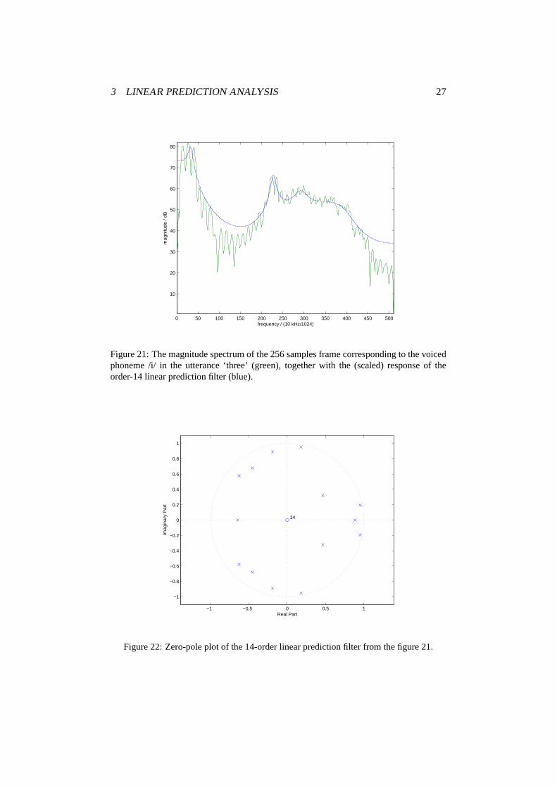
Figure 21: The magnitude spectrum of the 256 samples frame corresponding to the voicedphoneme /i/ in the utterance ‘three’ (green), together with the (scaled) response of theorder-14 linear prediction filter (blue).

−1 −0.5 0 0.5 1

−1

−0.8

−0.6

−0.4

−0.2

0

0.2

0.4

0.6

0.8

1

14

Real Part

Imag

inar

y P

art

Figure 22: Zero-pole plot of the 14-order linear prediction filter from the figure 21.

3 LINEAR PREDICTION ANALYSIS 28

Matrix Rs is called autocorrelation matrix and the vectorr s is called autocorrela-tion vector.

(2.2.1) To start with, we can find the solution to the equation

Rs(m)a(m) = r s(m)

using the ‘brute force’, i.e. finding the inverse of the autocorrelationM×M matrix.The cost of this method is generallyO(M3).

We implemented this approach inMATLAB by finding the order-14 predictorfor the voiced phoneme /i/ in the utterance ‘three’ using the following commands

x = digits.three1;

m = 2756;

N = 256;

n = m-N+1:m;

M = 14;

[r,eta] = xcorr(x(n),M,’biased’);

Rx = toeplitz(r(M+1:2*M));

rx = r(M+2:2*M+1);

a = Rx\rx;

NFFT = 1024;

k = 1:NFFT/2;

X = fft(x(n).*hann(N),NFFT);

Theta = 1./fft([1; -a],NFFT);

plot(k,20*log10(abs([353*Theta(k) X(k)])))

On the figure 21 we plotted the response of the filter obtained using the calculatedlinear prediction coefficients together with the magnitude spectrum of the 265 sam-ples frame that we used. It is clear that the filter determines spectral envelope ofthe speech signal.

On the figure 22 we included the zero-pole plot of the obtained linear predictionfilter to see how in the all-pole model, poles are used to determine the shape of filterresponse.

(2.2.2) The energyξ (m) = 1N ∑∞

m=−∞ e2(n;m) of the prediciton residual se-quencee(n;m) is given byξ (m) = rs(0;m)− rT

s (m)a(m). For the solution in previ-ous question, this energy (relative tors(0;m)) is 1 - rx’*a/r(M+1) = 0.0373.

3.3 Levison-Durbin Recursion

Levison-Durbin recursion is an efficient way to solve the normal equationRs(m)a(m) = r s(m), exploiting the fact thatRs(m) is Toeplitz, symmetric, and pos-itive definite, and the right-hand sider s(m) has a special relation to the elements ofRs(m).

(2.3.1) MATLAB function durbin.m implements Levison-Durbin recursion.The input arguments are the vectorr containing autocorrelation coefficients andthe prediction orderM. The output arguments are estimated LP parameters in thevectora, prediction error energies in the vectorxi, and estimated reflection coeffi-cients in the vectorkappa.

3 LINEAR PREDICTION ANALYSIS 29

function [a,xi,kappa] = durbin(r,M)

kappa = zeros(M,1);

a = zeros(M,1);

xi = [r(1); zeros(M,1)];

for (j=1:M)

kappa(j) = (r(j+1) - a(1:j-1)’*r(j:-1:2))/xi(j);

a(j) = kappa(j);

a(1:j-1) = a(1:j-1) - kappa(j)*a(j-1:-1:1);

xi(j+1) = xi(j)*(1 - kappa(j)^2);

end

(2.3.2) Now we use functiondurbin.m to solve the same problem as in the task(2.2.1) To compare the output vectora from this function with the one obtainedusing the ‘brute force’ we printed the parameters in 15 decimal places, and couldsee the difference in the 1–2 last decimal places. In fact, the largest difference ofthe two corresponding parameters is2.6·10−13.

(2.3.3) The energyξ (m) of the prediction residual sequence should be non-increasing for the increasing model order i.e. the prediction should be improvingwith the increasing model order. We verified this by plotting thexi vector on thefigure 23.

The sequenceξ ( j)(m) can be used to determine when the sufficient model or-der has been reached, by for example by stopping the recursion when the slopeξ ( j)(m)−ξ ( j−1)(m)

j−( j−1) = ξ ( j)(m)−ξ ( j−1)(m) is small enough.

0 5 10 150

0.5

1

1.5

2

2.5

3

3.5

4

4.5x 10

4

model order

ener

gy o

f res

idua

l seq

uenc

e

Figure 23: The plot of the energyξ (m) of the prediction residual sequence for the increas-ing model order.

3 LINEAR PREDICTION ANALYSIS 30

(2.3.4-6) Those three tasks are concerned with the conversion between the lin-ear prediction parametersa(i;m) and theM reflected coefficientsκ(i;m). We wroteMATLAB functions that implement the conversion in both directions, and we testedthe conversion.

The maximal difference between corresponding parameters when convertingfrom linear prediction parametersa(i;m) to reflected coefficientsκ(i;m) was3.03·10−15, and the maximal difference when converting formκ(i;m) to a(i;m) was0. In conclusion, both the ‘brute force’ solution to the normal equations, andthe Levison-Durbin recursion give the same result, the difference is the efficiency.Levison-Durbin is much more efficient, and it solves normal equation inO(M2)steps.

3.4 Inverse Filtering Computation

The prediction error sequencee(n;m) can be obtained by filterings(n;m) throughthe estimated inverse system

e(n;m) = s(n;m)−M

∑i=1

a(i;m)s(n− i;m)

or in the Z-transform domain

E(z) = A(z)S(z), A(z) = 1−M

∑i=1

a(i)z−i

0 50 100 150 200 250

−400

−300

−200

−100

0

100

200

300

400

500

600

sample number

ampl

itude

, res

idua

l seq

uenc

e

Figure 24: Frame of 256 samples corresponding to the voiced phoneme /i/ in the utterance‘three’ (blue), together with the residual sequencee(n;m) of the order-14 linear predictionfilter (green).

3 LINEAR PREDICTION ANALYSIS 31

(2.4.1) We found the residual sequencee(n;m) for the order-14 predictor fromthe task (2.2.1) by inverse filtering and we plotted it on the figure 24 together withthe amplitude waveform of the original frame. Impulse train excitation sequence iseasily recognizable from the residual sequence.

(2.4.2)MATLAB functionlpcauto.m preforms frame based linear predictionanalysis on a speech signa. Input parameters are the signalx, the prediction orderM,the window functionwin, and the overlap between adjacent framesOlap. Functionreturns linear prediction coefficients in the matrixar, prediction error energies inthe matrixxi, residual signal in the vectore, and the index of the last sample ineach frame in the vectorm.

function [ar,xi,e,m] = lpcauto(x,M,win,Olap)

Nx = length(x);

N = length(win);

if (N == 1)

N = win;

win = ones(N,1);

end

F = fix((Nx-Olap)/(N-Olap));

ar = zeros(M+1,F);

xi = zeros(M+1,F);

e = zeros(Nx,1);

m = zeros(F,1);

n = 1:N;

n1 = 1:Olap;

n2 = N-Olap+1:N;

n3 = Olap+1:N;

win1 = win(n1)./(win(n1)+win(n2)+eps);

win2 = win(n2)./(win(n1)+win(n2)+eps);

for (f=1:F)

[r,eta] = xcorr(x(n).*win,M,’biased’);

[a,xi(:,f),kappa] = durbin(r(M+1:2*M+1),M);

ar(:,f) = [1; -a];

ehat = filter(ar(:,f),1,x(n));

e(n) = [e(n(n1)).*win2 + ehat(n1).*win1; ehat(n3)];

m(f) = n(N);

n = n + (N-Olap);

end

(2.4.3) We applied functionlpcauto.m to the speech signal ‘She had your darksuit in greasy wash water all year’, using half overlapping Hann windows of length256 samples, and prediction order 14. On the figure 25 we plotted the amplitudewaveform of the speech signal, together with residual sequence.

By listening to residual sequence we concluded that sf one din’t know the orig-inal signal beforehand, it would be hard to understand residual sequence. Knowing

3 LINEAR PREDICTION ANALYSIS 32

0 1 2 3 4 5

x 104

−0.8

−0.6

−0.4

−0.2

0

0.2

0.4

0.6

0.8

1

sample number

ampl

itude

, res

idua

l seq

uenc

e

Figure 25: Amplitude waveform of the speech signal ‘She had your dark suit in greasywash water all year’ (blue), together with the residual sequence of the order-14 linearprediction filter (green).

the original speech signal, we could still understand it, which implies that some ofthe vocal tract spectrum is passing through the inverse filter. We could hear that theresidual sequence is quite clear for the sounds /S/ as in ‘she’, ‘wash’ and /s/ as in‘suit’, ‘greasy’. This can also be observed on the plot where we see that for thosesounds, residual sequence has relatively high amplitudes relative to original signal.

3.5 Formant Estimation

Formant frequencies and bandwidths are principal analytical features of the speechspectrum, and a simple technique for formant estimation could be based on peakfinding in an LP-derived magnitude spectrum. It is easier to find peaks of the LP-derived magnitude spectrum, than to estimate formants directly from the spectrumof the sound.

(2.5.1)MATLAB functionlpcplot.m makes a 2D plot of the magnitude spec-trum, if an input is a vector of LP coefficients, or it makes a 3D mesh plot ofmagnitude spectra, if an input is a matrix of LP coefficients.

function lpcplot(A,Nfft,Fs,m)

[M,N] = size(A);

if (N==1)

[Theta,F] = freqz(1,A,Nfft,Fs);

plot(F,20*log10(abs(Theta)));

xlabel(’Frequency, {\it F} [Hz]’);

ylabel(’Magnitude, |\theta(\omega)| [dB]’);

3 LINEAR PREDICTION ANALYSIS 33

0 1000 2000 3000 4000 5000 6000 7000 8000 9000 10000−1

−0.8

−0.6

−0.4

−0.2

0

0.2

0.4

0.6

0.8

1

sample number

ampl

itude

Figure 26: A plot of larger frame (38· 256 samples) taken from the utterance plotted atfigure 26 (sample numbers 9216–18944), corresponding to the segment ‘your dark s. . . ’.

Figure 27: A 3D mesh plot containing the LP-derived magnitude spectra of 76 half-overlapping frames of 256 samples corresponding to the utterance plotted at figure 26.

3 LINEAR PREDICTION ANALYSIS 34

else

Theta = zeros(Nfft,N);

for (n=1:N)

[Theta(:,n),F] = freqz(1,A(:,n),Nfft,Fs);

end

MeshHndl = meshz(m,F,20*log10(abs(Theta)));

axis ij; view(-45,45); set(MeshHndl,’MeshStyle’,’Column’);

axis tight; axis ’auto y’; axis ’auto z’;

xlabel(’Sample Number, {\it n}’);

ylabel(’Frequency, {\it F} [Hz]’);

zlabel(’Magnitude, |\theta(\omega)| [dB]’);

end

(2.5.2) Now we can look at the LPC spectra for a number of frames correspondingto the segment ‘your dark s. . . ’ (frames 71-147) taken from the the utterance weanalyzed in (2.4.3).

On the figure 26 we have a plot of amplitude waveform of the segment wewill consider. On the figure 27 we have a 3D mesh plot containing the LP-derivedmagnitude spectra of 76 half-overlapping frames of 256 samples, which correspondto our segment. On the figure 28 we have isolated three specific frames, and plottedthe LP-derived magnitude spectrum for each. Those frames correspond to voicedsound /u/ in ‘your’, voiced sound /a/ in ‘dark’, and unvoiced sound /s/ in ‘suit’.

Both on figure 27 and the first two plots in figure 28 we can observe that thebandwidth of the formants typically increases with its central frequency—formantsof lower frequencies will have more pointed and narrower peaks, while the for-mants on higher frequencies typically have flatter and wider peaks.

0 2000 4000 6000 8000−30

−20

−10

0

10

20

30

40

Frequency, F [Hz]

Mag

nitu

de, |

θ(ω

)| [

dB]

0 2000 4000 6000 8000−30

−20

−10

0

10

20

30

40

Frequency, F [Hz]

Mag

nitu

de, |

θ(ω

)| [

dB]

0 2000 4000 6000 8000−15

−10

−5

0

5

10

15

20

Frequency, F [Hz]

Mag

nitu

de, |

θ(ω

)| [

dB]

Figure 28: Plots of LP-derived magnitude spectra of three 256 sample frames from theutterance ‘your dark s. . . ’. Top left: corresponding to sound /u/ in ‘your’, top right: corre-sponding to sound /a/ in ‘dark’, bottom: corresponding to sound /s/ in ‘suit’.

3 LINEAR PREDICTION ANALYSIS 35

3.6 Pitch and Gain Estimation

The autocorrelation function of the prediction error sequencee(n;m) can be usedto estimate the pitch period for voiced frames as

maxη

re(η ,m), η 6= 0

If this peak value is below some threshold based on the total residual energy,for example0.25re(0;m) the frame is unvoiced.

(2.6.1) We used the autocorrelation of the residual sequencee(n;m)) for theorder-14 predictor of the voiced phoneme /i/ in the utterance ‘three’ to estimate thepitch.

On the figure 29 we plotted the autocorrelation of the residual sequence. Notconsidering the high peak atre(0), the autocorrelation reaches maximum for thetime shift η = 79. We got exactly the same result by looking at the short-timeautocorrelation of the original signal in the exercise (2.1.4), figure 20. We cal-culated there that the discrete periodη = 79 corresponds to the pitch frequencyFP = 10 kHz

79 = 126 Hz. That is a valid value for the pitch frequency, so the abovedescribed method of pitch estimation is useful.

However, in this example we have the problem that the peak value is rathersmall relative to the total residual energy (300 : 1600) so if the threshold value is0.25 this frame will be labeled unvoiced.

(2.6.2)MATLAB functionlpcpitch.m implements pitch estimation by findingthe maxima of residual sequence. The thresholdth is used for voiced/unvoiceddecision, and the peak search is preformed in the rangeminlag to maxlag.

−250 −200 −150 −100 −50 0 50 100 150 200 250−200

0

200

400

600

800

1000

1200

1400

1600

time shift

auto

corr

elat

ion

Figure 29: Short-term autocorrelation over the range[−250,250] of the residual sequencee(n;m)) for the order-14 predictor of the voiced phoneme /i/.

3 LINEAR PREDICTION ANALYSIS 36

function P = lpcpitch(e,m,N,th,minlag,maxlag)

F = length(m);

P = zeros(F,1);

for (f=1:F)

n = m(f)-N+1:m(f);

[re,eta] = xcorr(e(n),maxlag,’biased’);

[remax,idx] = max(re(maxlag+minlag+1:2*maxlag+1));

if (remax > th*re(maxlag+1))

P(f) = eta(maxlag+minlag+idx);

end

end

(2.6.3) We applied functionlpcpitch.m to the residual signal obtained from LPanalysis of the speech signal ‘She had your dark suit in greasy wash water all year’,and we plotted the results on the figure 30.

This pitch estimation method is rather simple to use, comparing to the pitchestimation from the task (1.6.3). Limiting the peak search to the rangeminlag tomaxlag, limits the search in a certain frequency range, automatically disregardingpitch values that are outside the expected range. But, as we have seen in the task(2.6.2), this method can also give wrong result.

The LP modeling problem focuses on the minimum-phase component in thespeech production system. However, the gainΘ0(m) accros frames are also impor-tant, and can be estimated from the prediction error energyξ (m) and pitch periodNp as

Θ0(m)≈√

ξ (m), unvoiced case

Θ0(m)≈√

Npξ (m), voiced case

(2.6.4) MATLAB function lpcgain.m implements gain estimation. Functiontakes as inputs the prediction error energy in vectorxi and the pitch period invectorP, and it returns the gain in the vectorG.

function G = lpcgain(xi,P)

F = length(xi);

G = zeros(F,1);

for (f=1:F)

if (P(f))

G(f) = sqrt(P(f)*xi(f));

else

G(f) = sqrt(xi(f));

end

end

(2.6.5) We applied functionlpcgain to the signal ‘She had your dark suit in greasywash water all year’, and we plotted the results on the figure 31.

(2.6.6)MATLAB functionlpcsyn performs speech synthesis from LP parame-ters. Function takes as inputs the LP coefficients in the matrixA, pitch period in the

3 LINEAR PREDICTION ANALYSIS 37

0 1 2 3 4 5

x 104

−0.5

0

0.5

1

0 1 2 3 4 5

x 104

90

100

110

120

130

140

Figure 30: Speech signal ‘She had your dark suit in greasy wash water all year’. Top:amplitude waveform, bottom: result of applying pitch estimation functionlpcpitch.mto the signal. Threshold value used for voiced/unvoiced segmentation was 0.18, and peaksearch was done in lag range 100 to 200, which corresponds to frequencies 80 Hz to 160Hz.

0 1 2 3 4 5

x 104

−0.5

0

0.5

1

0 1 2 3 4 5

x 104

0.05

0.1

0.15

0.2

0.25

Figure 31: Speech signal ‘She had your dark suit in greasy wash water all year’. Top:amplitude waveform, bottom: result of applying gain estimation functionlpcgain.m tothe signal.

3 LINEAR PREDICTION ANALYSIS 38

vectorP, gain in the vectorG, and the vectorm with the indices of the last samplein each frame. Function returns synthesized speech signalehat.

function xhat = lpcsyn(A,P,G,m)

F = length(m);

N = m(2) - m(1);

xhat = [];

for (f=1:F)

if (P(f))

e = zeros(N,1); e(1:P(f):N) = 1;

else

e = randn(N,1);

end

xhat = [xhat; filter(G(f),A(:,f),e)];

end

(2.6.7) By listening to the synthesized speech we concluded that it is easily un-derstandable, but also very different from the original signal, somehow monotone.Synthesized speech lacks quick variations that make the real speech lively.

3.7 Homework

We consider a toy example where the vocal tract system has orderM = 2, i.e., thespeech signals(n) is modeled by an AR(2) process with coefficientsa1 anda2.

(2.7.1)To sketch the IIR filter for the considered vocal tract model, we firstlooked at the filter

Θ(z) =S(z)E(z)

=1

1−a1z−1−a2z−2

and than we looked at what do we have in the time domain

s(n) = a1s(n−1)+a2s(n−2)+e(n)

so the block diagram looks like following illustration

- -

¾¾

¾

?

?6

6µ´¶³

µ´¶³ z−1

z−1

+

+a1

a2

e(n) s(n)

3 LINEAR PREDICTION ANALYSIS 39

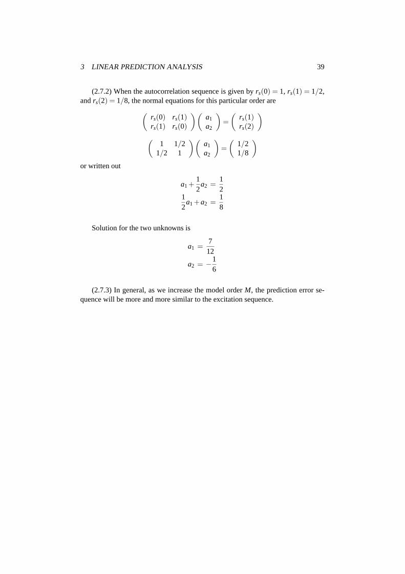
(2.7.2) When the autocorrelation sequence is given byrs(0) = 1, rs(1) = 1/2,andrs(2) = 1/8, the normal equations for this particular order are

(rs(0) rs(1)rs(1) rs(0)

)(a1

a2

)=

(rs(1)rs(2)

)

(1 1/2

1/2 1

)(a1

a2

)=

(1/21/8

)

or written out

a1 +12

a2 =12

12

a1 +a2 =18

Solution for the two unknowns is

a1 =712

a2 = −16

(2.7.3) In general, as we increase the model orderM, the prediction error se-quence will be more and more similar to the excitation sequence.

4 SPEECH CODING AND SYNTHESIS 40

4 Speech Coding and Synthesis

4.1 Perceptual Weighting Filter

Linear prediction analysis estimates the all-pole (vocal-tract) filter for each frameof the signal. The synthesized speech is then generated by exciting vocal tract fil-ter. The difference between the synthesized speech and original speech constitutesan error signal that will be minimized by optimizing the excitation signal. Prior tominimization, error signal is spectrally weighted to emphasize perceptually impor-tant frequencies.

Functionlpcana performs LP analysis on the speech frame using Levison-Durbin recursion, and functionlpcweight returns the coefficients of the percep-tual weighting filter.

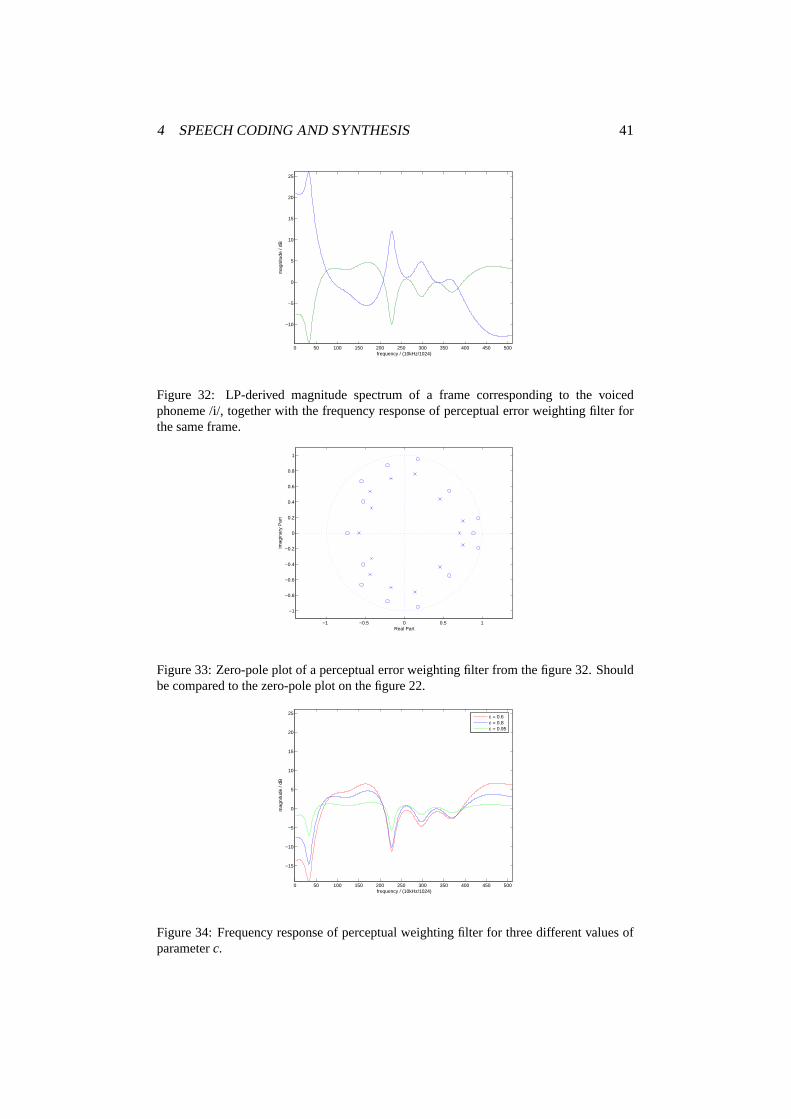
(3.2.2) We performed LP analysis on the voiced phoneme /i/ in the utterance‘three’ using order-14 prediction, and we found the corresponding perceptual errorweighting filter forc = 0.8.

load digits;

x = digits.three1;

m = 2756;

N = 200;

n = m-N+1:m;

M = 14;

[ar,xi,kappa,ehat] = lpcana(x(n),M);

c = 0.8;

ac = lpcweight(ar,c);

Nfft = 1024;

k = 1:Nfft/2;

Theta = 1./fft(ar,Nfft);

W = fft(ar,Nfft)./fft(ac,Nfft);

plot(k,20*log10(abs([Theta(k) W(k)])))

zplane(ar’,ac’)

On the figure 32 we plotted LP-derived magnitude spectrum of a frame, togetherwith the frequency response of perceptual error weighting filter for the same frame.We can see that the perceptual error weighting filter de-emphasizes formant fre-quencies.

On the figure 33 we have zero-pole plot of a perceptual error weighting filter.By comparing it to the zero-pole plot of the linear prediction filter on figure 22,we can see how the perceptual weighting filter is obtained by placing zeros at thepositions where LP filter has poles, and adding corresponding poles at the distancedetermined by parameterc.

On the figure 34 we have plotted the frequency response of perceptual weight-ing filter for three different values of parameterc. If the valuec is close to 1, fre-quency response of the filter is rather flat—it is not doing a lot of filtering. Whenthe value ofc decreases, filtering becomes more pronounced. The optimal value ofc (around 0.8) depends on the human perception.

4 SPEECH CODING AND SYNTHESIS 41

0 50 100 150 200 250 300 350 400 450 500

−10

−5

0

5

10

15

20

25

frequency / (10kHz/1024)

mag

nitu

de /

dB

Figure 32: LP-derived magnitude spectrum of a frame corresponding to the voicedphoneme /i/, together with the frequency response of perceptual error weighting filter forthe same frame.

−1 −0.5 0 0.5 1

−1

−0.8

−0.6

−0.4

−0.2

0

0.2

0.4

0.6

0.8

1

Real Part

Imag

inar

y P

art

Figure 33: Zero-pole plot of a perceptual error weighting filter from the figure 32. Shouldbe compared to the zero-pole plot on the figure 22.

0 50 100 150 200 250 300 350 400 450 500

−15

−10

−5

0

5

10

15

20

25

frequency / (10kHz/1024)

mag

nitu

de /

dB

c = 0.6c = 0.8c = 0.95

Figure 34: Frequency response of perceptual weighting filter for three different values ofparameterc.

4 SPEECH CODING AND SYNTHESIS 42

4.2 Excitation Sequence

The signal used to excite the LP synthesis filter is determined dynamically fewtimes in each frame. An excitation sequence is first selected from the codebookand a long-delay correlation filter is used to generate the pitch periodicity. Pitchand gain are found by performing an exhaustive search on the certain range, andthe codebook vector is found by performing an exhaustive search of the codebookto minimize the energy of perceptually weighted error.

(3.3.1) We generated a Gaussian codebook containing 1024 sequences of length40 by using following commands.

randn(’state’,0);

cb = randn(40,1024);

4.3 CELP Synthesizer

CELP coder estimates model parameters from frames of speech, encodes and trans-mits the parameters to the receiver on a frame-to frame basis. The speech signalis than reconstructed at the receiver. Parameters being transmitted between CELPcoder and decoder are: estimated reflection coefficients, gain, index of the code-book vector, scale factor (excitation parameter used for long-delay correlation fil-ter) and pitch.

CELP synthesizer consists of the cascade of the pitch synthesis filter and theLP synthesis filter. The excitation signal is taken from the codebook of storedsequences.

MATLAB function celpsyn.m implements the CELP synthesizer, while theMATLAB functioncelpana implements the CELP coder.

(3.4.2) We applied the functionscelpana.m and celpsyn.m to the singlespeech frame, i.e. we first coded and than synthesized the speech frame.

load digits;

x = digits.three1;

m = 2756;

N = 200;

n = m-N+1:m;

L = 40;

M = 12;

c = 0.8;

Pidx = [16 160];

bbuf = 0;

ebuf = zeros(N,1);

Zf = [];

Zw = [];

[kappa,k,theta0,P,b,ebuf,Zf,Zw] = ...

celpana(x(n),L,M,c,cb,Pidx,bbuf,ebuf,Zf,Zw);

[xhat,ebuf,Zi] = celpsyn(cb,kappa,k,theta0,P,b,ebuf,[]);

plot([xhat x(n)])

4 SPEECH CODING AND SYNTHESIS 43

0 20 40 60 80 100 120 140 160 180 200−600

−400

−200

0

200

400

600

Figure 35: A 256 samples frame corresponding to the voiced phoneme /i/ in the utter-ance ‘three’ (blue) together with the frame obtained by CELP coding/decoding the signal(green).

On the figure 35 we plotted the original speech frame, and the synthesized frame.The similarities between the synthesized and original speech frame are obvious,but we can also notice that the synthesized signal has a stronger ‘attack’ than theoriginal signal.

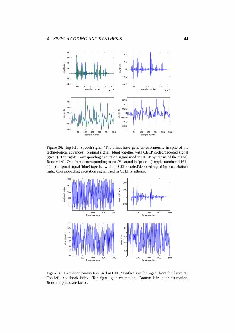
(3.4.4)MATLAB functioncelp.m preforms frame base CELP coding and syn-thesis on speech signals. We applied this function to the speech signal ‘The priceshave gone up enormously in spite of the technological advances’.

randn(’state’,0);

cb = randn(40,1024);

load ma1_1;

x = ma1_1;

N = 160;

L = 40;

M = 10;

c = 0.8;

Pidx = [16 160];

[xhat,e,k,theta0,P,b] = celp(x,N,L,M,c,cb,Pidx);

plot([x xhat])

On the figure 36 we can see the original speech signal and the synthesized speechsignal. By listening to the synthesized speech, we concluded that the quality of thesynthesized speech is good—it sounds quite natural. We have plotted the excitationsignal, and we can see that its shape resembles the shape of the speech signal.

We have also extracted one frame corresponding to the /Y/ sound in ‘prices’and plotted the original signal together with the synthesized. Now it is easier tonotice how good the synthesized signal approximates the original. We can alsobetter see the excitation signal for a voiced segment. We concluded that the exci-tation signal isn’t just a pulse train—it looks more like as if the part of the speech

4 SPEECH CODING AND SYNTHESIS 44

0.5 1 1.5 2 2.5 3

x 104

−0.4

−0.2

0

0.2

0.4

0.6

0.8

sample number

ampl

itude

0.5 1 1.5 2 2.5 3

x 104

−0.2

−0.1

0

0.1

0.2

sample number

ampl

itude

50 100 150 200 250 300−0.4

−0.2

0

0.2

0.4

0.6

sample number

ampl

itude

50 100 150 200 250 300

−0.15

−0.1

−0.05

0

0.05

0.1

0.15

sample number

ampl

itude

Figure 36: Top left: Speech signal ‘The prices have gone up enormously in spite of thetechnological advances’, original signal (blue) together with CELP coded/decoded signal(green). Top right: Corresponding excitation signal used in CELP synthesis of the signal.Bottom left: One frame corresponding to the /Y/ sound in ‘prices’ (sample numbers 4161–4460), original signal (blue) together with the CELP coded/decoded signal (green). Bottomright: Corresponding excitation signal used in CELP synthesis.

200 400 600 800

200

400

600

800

1000

frame number

code

book

inde

x

200 400 600 800

−0.02

0

0.02

0.04

frame number

gain

est

imat

ion

200 400 600 80020

40

60

80

100

120

140

160

frame number

pitc

h es

timat

ion

200 400 600 8000

0.2

0.4

0.6

0.8

1

1.2

frame number

scal

e fa

ctor

Figure 37: Excitation parameters used in CELP synthesis of the signal from the figure 36.Top left: codebook index. Top right: gain estimation. Bottom left: pitch estimation.Bottom right: scale factor.

4 SPEECH CODING AND SYNTHESIS 45

signal is present in the excitation signal. We verified this conclusion by listeningto excitation signal.

On the figure 37 we have plotted excitation parameters: codebook index, gainestimation, pitch estimation and scale factor that controls amounts of the contri-bution from the codebook sequence and from an interval of past excitation. Asexpected, codebook indexes are chosen random-like. Gain reflects the shape of thesignal, since gain is connected to the amplitude/energy. Pitch estimation is not re-sulting in a nice pitch curve, and it seems hard to determine pitch from the sequenceof pitch estimations. Scale factor is also not providing any obvious information.

(3.4.5) We repeated the experiment using LPC model orderM = 14. By listen-ing to this synthesized speech signal, we couldn’t hear any improvement. However,listening to the difference of the two signals (i.e. one signal subtracted from theother) verified our expectation that higher model order has to improve signal ap-proximation.

We also repeated experiment using model orderM = 2, and we were surprisedto hear quite muffed, but still understandable speech signal.

(3.4.6) We repeated the experiment modifying the perceptual weighting coeffi-cientc. We used a few different values between 0 and 1, but could not hear a bigimprovement/degradation of the synthesized speech. Even usingc = 1 (no percep-tual weighting at all) didn’t decrease the quality of the signal significantly, or atleast not so much that we could hear it. On the other hand, using the same methodas in the previous task, and listening to differences between signals, confirms thatthe difference exists.

(3.4.7) We also tried modifying codebook size and the length of the randomsignals in the codebook. We noticed that the size of the codebook greatly influencesthe speed of the computation. For example, reducing the number of vectors from1024 to 256 reduced the computational time from 13 to 6 seconds. This is easy tounderstand—initial excitation sequence is found by preforming exhaustive searchof the codebook, so it must take longer time to search longer codebook. The lengthof the vectors is not influencing computational time so strongly—having shorterframes means having more frames.

As for the quality, again we didn’t hear any significant improvement/degrada-tion of the speech signal when modifying the number or the length of the vectors.

4.4 Quantization

Because of limited bandwidth between coder and decoder, the parameters obtainedby CELP coder are first quantized according to the bit allocation table and thantransmitted.

(3.5.2) Functioncelp16k.m implements 16000 bps CELP coder and we ap-plied it to the speech signal ‘The prices have gone up enormously in spite of thetechnological advances’. On the figure 38 we plotted the original signal togetherwith coded/encoded signal. By listening to synthesized speech signal, we couldyet again not hear any significant degradation.

4 SPEECH CODING AND SYNTHESIS 46

0.5 1 1.5 2 2.5 3

x 104

−0.4

−0.2

0

0.2

0.4

0.6

0.8

sample number

ampl

itude

0.5 1 1.5 2 2.5 3

x 104

−0.4

−0.2

0

0.2

0.4

0.6

0.8

sample number

ampl

itude

Figure 38: Speech signal ‘The prices have gone up enormously in spite of the technologicaladvances’, original signal (blue) together with the synthesized signal (green). Left: using16000 bps CELP coder/decoder. Right: using 9600 bps CELP coder/decoder.

(3.5.4) Functioncelp9600k.m implements 9600 bps CELP coder. We re-peated the experiment by applying functioncelp9600k.m to the speech signal.We plotted the original and coded/decoded signal on the figure 38. By listeningto the synthesized signal we did observe degradation—signal was muffed, but stillvery understandable.

4.5 Homework

(3.6) We should discuss the improvements of the LPC based vodocoders that canbe obtained by using linear interpolation of adjacent frame parameters.

Using linear interpolation of adjacent frame parameters is surely not influenc-ing the transmission bandwidth of the LP parameters, since interpolation is doneonly on the decoding side. So there is a good chance that interpolation could beefficient (and bandwidth ‘cheap’) way to improve the quality of the synthesizedsignal. The question is still whether using interpolation actually improves the syn-thesized signal quality.

We know that LP coefficients in adjacent frames can change rapidly. Linear in-terpolation of LP coefficients would result in smoother variation of LP coefficients.It is possible that the rapid change of LP coefficients introduces some unwanted ef-fects and interpolation could help in that case. On the other hand, it is also possiblethat smoothing of LP parameters would result with unwanted flatness. Experimentis a way to solve this dilemma.

5 SPEECH RECOGNITION 47

5 Speech Recognition

5.1 Feature Extraction

Feature vector sequence for each frame are usually obtained from the LP parame-ters. In our exercise, the feature vector is composed of 12 cepstral coefficients and12 difference cepstral coefficients.

Functionhmmfeatures.m performs feature extraction procedure on a speechsignal.

(4.1.2) We verified functionhmmfeatures.m on the speech signal ‘one’ usingthe following commands.

load digits;

s = digits.one1;

N = 320;

deltaN = 80;

M = 12;

Q = 12;

y = hmmfeatures(s,N,deltaN,M,Q);

plot(y)

On the figure 39 we can see the obtained feature vectors. Each feature vector iscomposed of 12 cepstral coefficients and 12 differenced cepstral coefficients, andwe can see that cepstral coefficients are rather dependant on each other—a lot ofvectors has the same value for the first 3 features. Differenced cepstral coefficientsare not so dependant on each other.

We assumed that cepstral coefficients change slowly from frame to frame, andto verify that on the figure 40 we plotted the change of feature values from frame

2 4 6 8 10 12 14 16 18 20 22 24

−4

−2

0

2

4

6

8

feature number

feat

ure

valu

e

Figure 39: Feature vectors extracted form speech signal ‘one’. There are in total 54 featurevectors corresponding to 54 overlapping frames. Feature numbers 1–12: cepstrum, featurenumbers 13–24 differenced cepstrum.

5 SPEECH RECOGNITION 48

10 20 30 40 50

−4

−2

0

2

4

6

8

frame number

feat

ure

valu

e

10 20 30 40 50−1.5

−1

−0.5

0

0.5

1

1.5

frame number

feat

ure

valu

e

Figure 40: Change of feature values from frame to frame. Left: 12 cepstral coefficients,right: 12 differenced cepstral coefficients.

to frame. We can see that our assumption was true, and we can also see that thedifferenced cepstral coefficients change rapidly in time.

5.2 Vector Quantization

We want to use HMM with a discrete observation symbol instead of continuousvectors shown on the figure 39. Therefor we use functionkmeans.m that imple-ments vector quantization algorithm. For each word, the feature extraction consti-tutes an observation sequence of 24 dimensional vectors, which are than quantizedinto one of the permissible set resulting in the scalar, discrete observation sequence.

Functionkmeans implements k-means vector quantization algorithm.(4.2.2) We verified thekmeans function on 2 dimensional random vectors be-

cause it is easier to visualize the process of quantization in 2 dimensions.

Y = randn(1000,2);

K = 10;

maxiter = 500;

[Yc,c,errlog] = kmeans(Y,K,maxiter);

Yc

figure, hold on,

plot(Y(c==1,1),Y(c==1,2),’.’,Y(c==2,1),Y(c==2,2),’.’,...

Y(c==3,1),Y(c==3,2),’.’,Y(c==4,1),Y(c==4,2),’.’,...

Y(c==5,1),Y(c==5,2),’.’,Y(c==6,1),Y(c==6,2),’.’,...

Y(c==7,1),Y(c==7,2),’.’,Y(c==8,1),Y(c==8,2),’.’,...

Y(c==9,1),Y(c==9,2),’.’,Y(c==10,1),Y(c==10,2),’.’,’MarkerSize’,10)

for i=1:10, text(Yc(i,1),Yc(i,2),num2str(i),’FontWeight’,’bold’), end,

axis([-2.5,2.5,-2.5,2.5])

We plotted the result of quantization on the figure 41.Functionhmmcodebook.m makes a codebookcb containing feature vector pro-

totypes based on training sequences defined by the cell-array containing words thatwill be used for training. For each word, a frame based analysis is performed usinghmmfeatures.m to give observation vectors. The feature vectors for all words are

5 SPEECH RECOGNITION 49

−2.5 0 2.5−2.5

0

2.5

1

2

3

4

56

7

8

9

10

Figure 41: Result of performing vector quantization of 1000 random points. Centroidsare marked with the cluster number, and vector points assigned to a certain cluster arerepresented with dots of the same color.

2 4 6 8 10 12 14 16 18 20 22 24

−3

−2

−1

0

1

2

3

4

5

6

feature number

feat

ure

valu

e

Figure 42: Feature vector prototypes (codebook vectors) obtained by vector quantizationof the feature vectors extracted from the training set consisting of 15 occurrences of eachspoken word ‘zero’ to ‘nine’. Feature vectors were quantized into 16 clusters. Featurenumbers 1–12: cepstrum, feature numbers 13–24 differenced cepstrum.

5 SPEECH RECOGNITION 50

than concatenated and vector quantized intoK feature vector prototypes, whereK< Kmax.

(4.2.5) We generated a codebook from a training set of 15 occurrences of eachof spoken words ‘zero’ to ‘nine’ using following commands.

load ti46;

data = ti46.case(27:36);

N = 320;

deltaN = 80;

M = 12;

Q = 12;

Kmax = 16;

[cb,K,T,dist] = hmmcodebook(data,N,deltaN,M,Q,Kmax);

plot(cb)

On the figure 42 we can see the resulting 16 vector prototypes. We can see thatthe vector prototypes are not as dependent as the feature vectors from a single word.To cover the whole training set, the feature vectors need to show more variation andneed to be on a certain distance one from another.

(4.2.6) One measure of the quality of a codebook is the average distance of anobservation vector in the training data from its corresponding symbol. We checkedhow does the distortion depend on the codebook sizeK using following commands.

load ti46;

data = ti46.case(27:36);

N = 320;

deltaN = 80;

M = 12;

Q = 12;

Kmax = [2 4 8 16 32];

dist = zeros(1,length(Kmax));

for i=1:length(Kmax)

[cb,K,T,dist(i)] = hmmcodebook(data,N,deltaN,M,Q,Kmax(i));

end

plot(Kmax, dist)

0 10 20 300.02

0.025

0.03

0.035

0.04

0.045

0.05

codebook size

quan

tizat

ion

dist

ortio

n

Figure 43: Quantization distortion versus codebook size for the feature vectors extractedfrom the training set consisting of 15 occurrences of each spoken word ‘zero’ to ‘nine’.

5 SPEECH RECOGNITION 51

On the figure 43 we can see that, as expected, distortion decreases with increas-ing codebook size. Since a larger codebook implies more computation (increasedsize ofK×S observation probability matrixB), there is an incentive to keep thecodebook as small as possible without jeopardizing recognition ability. Based onthese two conditions, the reasonable codebook size is guided by the experimentevidence. When implementing the quantization, it can be decided that the desiredcodebook size is reached when the curve of distortion versus codebook size is flatenough.

5.3 Training the HMM

Training the HMM for its dedicated word means using the training words to es-timate state transition matrixA, observation probability matrixB and state proba-bility vector π(1). The aim is to maximize probability of a HMM to produce it’sdedicated word. This is done iteratively using the forward-backward reestimationalgorithm until the desired tolerance is reached. We also need to train for the sameword multiple times.

Functionhmmfb.m implements F-B algorithm and functionhmmtrain.m im-plements iterative training of multiple HMM’s based on the feature extraction, vec-tor quantization, and F-B algorithm.

(4.3.5) We generated a codebook from a training set of 10 occurrences of eachof the spoken words ‘zero’ to ‘nine’. The codebook was then used to train a set often HMM’s each having 5 hidden states.

load ti46;

data = ti46.case(27:36);

for(i=1:10)

train{i} = data{i}(1:10);

end

N = 320;

deltaN = 80;

M = 12;

Q = 12;

Kmax = 16;

[cb,K,T,dist] = hmmcodebook(train,N,deltaN,M,Q,Kmax);

S = 5;

maxiter = 5000;

tol = 1e-3;

[A_m,B_m,pi_m,loglike_m] = hmmtrain(train,N,deltaN,M,Q,cb,S,maxiter,tol);

plot(loglike_m{1})

plot(loglike_m{6})

We can observe the log-likelihood as function of the iteration number in the F-B reestimation algorithm on the figures 44 where we plotted log-likelihoods com-puted when building HMM’s for recognizing words ‘one’ and ‘six’. We can seethat it took 16 iterations to build satisfactory model for the word ‘one’ and 17 iter-ations to build the model for word ‘six’. We can conclude that the typical training

5 SPEECH RECOGNITION 52

0 5 10 15−500

−450

−400

−350

−300

−250

−200

iteration number

log−

likel

ihoo

d

0 5 10 15−450

−400

−350

−300

−250

−200

−150

iteration number

log−

likel

ihoo

d

Figure 44: Log-likelihood versus iteration number computed when building HMM’s forrecognizing the word ‘one’ (left), and the word ‘six’ (right).

length is around 20 iterations. Log-likelihoods reached the final, maximal value ofapproximately -250, which corresponds to probability of10−250.

We can also observe the structure of the matricesA andB.

mesh(A_m{1})

mesh(B_m{1})

We can see the mesh plot of matricesA andB on the figures 45 and 46. MatrixA has largest probabilities on the main diagonal. This means that if the process isin a certain state at the timet, the probability is highest that it will stay in that statein the timet +1. This implies that the states don’t change rapidly in time.

Looking at the visualization of matrixB on figure 46 we can see that for eachstate, there is just a couple of observations that have a high probability. Usually itis just one high probability per state. For example, for state 4 there is very highprobability of observing symbol 9, and for state 2 there a high probabilities ofobserving symbols 6 and 15. We can conclude that the hidden Markov model isnot totaly hidden.

The structure of matricesA andB is in accordance with our conclusion for thetask (4.1.2)—if the chance is big to stay in the present state, and if the chanceof observing a single symbol for each state is also big, then feature vectors willchange slowly in time.

5.4 Recognition using the HMM

For a given (but unknown) observation sequence and a given HMM trained oncertain word, we can calculate the log-likelihood that HMM produced a sequence.To recognize a given signal, we first have to utilizehmmfeatures.m to extract thefeature vectors. Than we use functionhmmlogp.m to calculate the log-likelihoodfor a given sequence and a given HMM. Finally, we have to find the HMM thatgives the highest probability of producing the sequence.

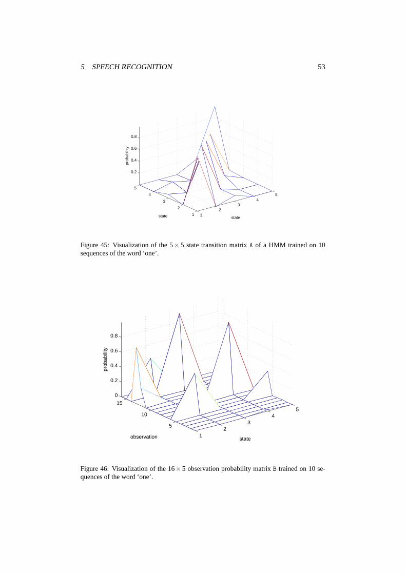
5 SPEECH RECOGNITION 53

12

34

5

1

2

3

4

5

0.2

0.4

0.6

0.8

statestate

prob

abili

ty

Figure 45: Visualization of the5× 5 state transition matrixA of a HMM trained on 10sequences of the word ‘one’.

12

34

5

5

10

15

0

0.2

0.4

0.6

0.8

stateobservation

prob

abili

ty

Figure 46: Visualization of the16×5 observation probability matrixB trained on 10 se-quences of the word ‘one’.

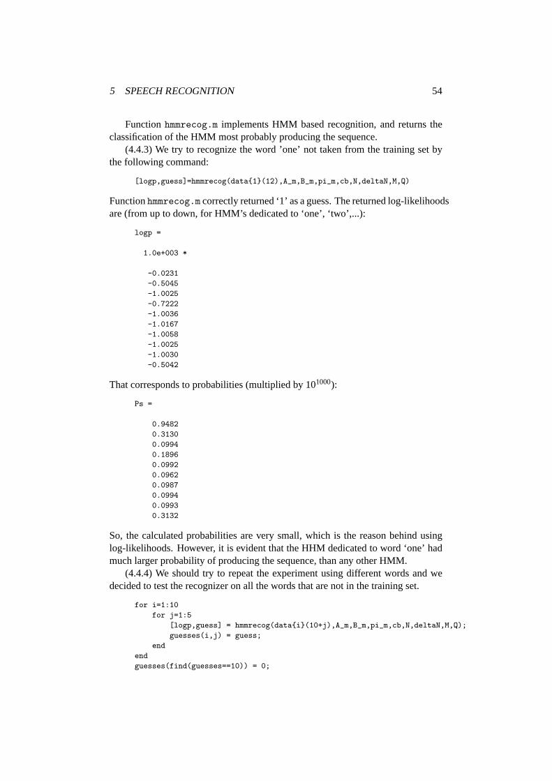
5 SPEECH RECOGNITION 54

Functionhmmrecog.m implements HMM based recognition, and returns theclassification of the HMM most probably producing the sequence.

(4.4.3) We try to recognize the word ’one’ not taken from the training set bythe following command:

[logp,guess]=hmmrecog(data{1}(12),A_m,B_m,pi_m,cb,N,deltaN,M,Q)

Functionhmmrecog.m correctly returned ‘1’ as a guess. The returned log-likelihoodsare (from up to down, for HMM’s dedicated to ‘one’, ‘two’,...):

logp =

1.0e+003 *

-0.0231

-0.5045

-1.0025

-0.7222

-1.0036

-1.0167

-1.0058

-1.0025

-1.0030

-0.5042

That corresponds to probabilities (multiplied by101000):

Ps =

0.9482

0.3130

0.0994

0.1896

0.0992

0.0962

0.0987

0.0994

0.0993

0.3132

So, the calculated probabilities are very small, which is the reason behind usinglog-likelihoods. However, it is evident that the HHM dedicated to word ‘one’ hadmuch larger probability of producing the sequence, than any other HMM.

(4.4.4) We should try to repeat the experiment using different words and wedecided to test the recognizer on all the words that are not in the training set.

for i=1:10

for j=1:5

[logp,guess] = hmmrecog(data{i}(10+j),A_m,B_m,pi_m,cb,N,deltaN,M,Q);

guesses(i,j) = guess;

end

end

guesses(find(guesses==10)) = 0;

5 SPEECH RECOGNITION 55

The returned matrix of guesses is

one two three four five six seven eight nine zero

1 2 3 4 5 6 7 8 9 0

1 2 3 4 5 6 7 8 9 0

1 2 3 4 5 6 7 8 9 0

1 2 3 4 5 6 7 8 9 0

1 2 3 4 5 6 7 8 9 0

So we can see that the recognizer had success rate of 100% on this set.(4.4.5) We repeated the experiments using various block size and spacing—

original size wasN = 320 anddeltaN = 80. We expected more wrong guessesasN anddeltaN increase, but the recognizer proved to be rather robust, and weneeded to increaseN up to 2000 anddeltaN up to 500 to get a few wrong results.We include results forN = 3200 anddeltaN = 800 where we can see the de-terioration in the quality of recognizing—word ‘nine’ was wrongly recognized as‘one’ in 4 out of 5 cases.

one two three four five six seven eight nine zero

1 2 3 4 5 6 7 8 1 0

1 2 3 4 5 6 7 8 1 0

1 2 3 4 5 6 7 8 9 2

1 2 8 4 5 6 7 8 1 0

9 2 3 4 5 6 7 8 1 0

We assume that the success rate will depend more on the block size and spacingfor recognizers that have to capture subtle difference between words, for examplefor medium size vocabularies recognizers. Longer frames do increaseimprove thecomputation speed, so again, one has to evaluate the computation speed and cor-rectness by experiment to solve this dilemma.

(4.4.6) We repeated the experiments using LPC/cepstrum coding of smallerand larger order—originally wasM = 12 andQ = 12. Success rate was generallysmaller for smaller order and the recognition was becoming more unstable, chang-ing the output from experiment to experiment. Still, we found the recognizer ratherrobust to the changes of LPC/cepstrum order. We include the results forM = 4 andQ = 4.

one two three four five six seven eight nine zero

1 5 5 4 5 6 7 6 9 0

1 2 3 4 5 6 7 8 9 0

1 2 3 4 5 6 7 8 9 0

1 2 3 4 5 6 7 8 9 0

1 5 5 4 5 6 7 6 9 0

(4.4.7) We repeated the experiments again, this time using codebooks of dif-ferent sizes—originally wasK = 16. Quantizing the feature vectors into smallernumber of clusters worsened the success rate. We include the results forK = 6.

5 SPEECH RECOGNITION 56

one two three four five six seven eight nine zero

1 2 8 2 5 6 0 8 9 0

1 2 3 4 5 6 0 8 1 0

1 2 3 4 5 6 7 8 9 0

1 2 8 4 5 6 7 8 9 0

1 2 3 4 5 6 7 8 9 0

In conclusion, the choice of parameters has to be determined by experiment, con-sidering the requirements for the specific speech recognizer.

5.5 Homework

(4.5) We should discuss improvements on the word classifier, based on what wehave learned during the course.

When changing the parameters of the word classifier we noticed that classifieroften makes two wrong guesses for a single word while guessing everything elsecorrectly. We assumed that the model for the word in question wasn’t optimizedcorrectly during training.

As we learned in the lesson, reestimation algorithm finds the model that givesthe local maximum of the probability, and finding global maximum is not ensured.So, the model found by reestimation algorithm depends on initial (random) pointof search.

The speech recognizer we implemented in the exercise is not taking this prob-lem into consideration. To improve the chances of finding the optimal model, rees-timation algorithm could be performed a number of times from different startingpoints used by F-B algorithm, and the best of the found models could be chosen.

REFERENCES 57

References

[1] Sadaoki Furui. Speech recognition technology in the ubiquitous/wearablecomputing environment.Proceedings of the 2000 IEEE International Con-ference on Acousitcs, Speech, and Signal Processing.

[2] John H. L. Hansen John R. Deller and John G. Proakis.Discrete-Time Process-ing of Speech Signals. IEEE Press, 2000.

[3] John G. Proakis and Dimitris G. Manolakis.Digital Signal Processing.Prentice-Hall, third edition, 1996.

[4] Thomas F. Quatieri.Discrete-Time Speech Signal Processing. Prentice-Hall,third edition, 1996.

[5] Andreas Spanias Ted Painter. Perceptual coding of digital audio.Proceedingsof IEEE, 88(4), April 2000.