Speculation and Hedging in Commodity Options: A Modification … · Speculation and Hedging in...

J ECO 8USN 201 1992; 44:201-221

Speculation and Hedging in Commodity Options: A Modification of Wolf's Portfolio Model

David W. Bullock and Dermot J. Hayes

This article modifies the Wolf (Journal o f Economics and Business 39:141-158, 1987) mean-variance portfolio model containing physicals, futures, and options. The modification is accomplished through an endogenization of the variance-covariance matrix of portfolio returns. This endogenization reduces the investor's informational input to two variables: the mean and variance of the future underlying price distribution. An analysis of the analytical form of the model basically supports the results of Wolf. However, because of the mathematical formulation of the model, the speculative and hedging effects of new information on the mean and variance can be separated out for analytical and simulation purposes.

I. Introduction Options are a versatile tool in the toolbox of the modern investor. An option contract can be combined with other option contracts and/or financial instruments, such as futures contracts, to tailor a customized pattern of returns. This allows the investor to take greater advantage of available private and public information. Prior to the introduction of options in late 1984, commodity investors lacked the means by which to profit from information on the variability of future prices. With the introduction of commodity options, investors can speculate on future variability by using variants of the "straddle" position.

Two-parameter certainty equivalent or mean-variance (EV) models have been used in the portfolio choice literature dating from the seminal work by Markowitz (1952). These models have found numerous applications in the analysis of futures markets (Johnson 1960; McKinnon 1967; Danthine 1978; Holthausen 1979; Stein 1985). However, there have been few applications of this framework to the study of option markets. An exception to this is Wolf (1987), who applied the EV model to the study of

Address reprint requests to David W. Bullock, Department of Agricultural Economics and Economics, Montana State University, 210 Linfield Hall, Bozeman, Montana 59717.

Journal of Economics and Business 0148-6195/92/$05.00 © 1992 Temple University

202 D.W. Bullock and D, J. Ha~es

optimal hedging and speculation decisions for a commodity investor using both futures and option contracts. The variance-covariance (VCV) matrix in Wolf's model is generic in form, with an ordinal specification of the relationships between the matrix components (i.e., the futures and option price moments). These relationships are specified using prior knowledge of the interaction between futures and options.

Wolf proved three theorems from the analytical form of his model. The first theorem states that a change in expected net speculative returns to futures will result in a larger cross-speculative effect for the option than the own-speculative effect for the futures. The second theorem states that a change in expected net speculative returns to the option will result in a larger own-speculative effect for the option than the cross-speculative effect for the futures. The third theorem states that, in the absence of basis risk, the futures contract is the preferred hedging instrument for physical inventory.

Wolf also set up his model in a simulation framework to examine the positions that would be taken by a commodity investor. The simulation model assumed that the investor's preferences could be represented by the hyperbolic absolute risk aversion (HARA) family of utility functions, and that the investor's subjective valuation of the option could be represented by Black's option pricing formula. The results of the simulation analysis showed that the investor would prefer positions that were variants of the short straddle position.

Wolf and Francis (1991) expanded upon the simulation analysis of WoWs article. From their simulation results, four general observations were made. First, they found that commodity options successfully compete against other contracts in the optimal portfolio. Second, they found that there was a discontinuity in the optimal position diagrams around the point where the option(s) was struck at-the-money. Third, they found that the slope of the optimal position diagram remained constant over a wide range of prices. Fourth, they found that the optimal portfolio would employ compli- cated hedges involving a combination of futures and options. Their analyses were based upon a simulation model that was constructed from Wolf's theoretical model. The parameters of the VCV matrix in the simulation were arbitrarily specified and based upon realistic assumptions of the interaction between options, futures, and spot markets. Wolf and Francis used the negative exponential, logarithmic, and quadratic specifica- tions of the investor's utility function.

In this paper, Wolf 's portfolio model is modified by endogenizing the VCV matrix of returns. This endogenization is facilitated by statistical theorems that allow for the derivation of the first two central moments for discontinuous functions of a random variable. The attractiveness of this model is that it allows for a comparative static analysis of the effects of investor information on the optimal portfolio positions. In particular, the investor's information set can be represented by estimates of the mean and variance of the statistical distribution of the underlying price. This, in turn, allows us to examine the response of investors to information that is not already incorporated into the option and futures prices.

This article is structured as follows. In the next section (II), the portfolio model is constructed with the assumption of no basis risk. Some comparative static results are derived from the analytical model and compared to those of Wolf. In Section III, the robustness of these results with respect to basis risk is examined. In Section IV, a simulation of the model without basis risk is used to examine the optimal positions taken by an investor. These positions will be compared with those contained in Wolf and Francis. The final section (V) will summarize the results of the previous sections.

Speculation and Hedging in Commodity Options 203

II. The Model Without Basis Risk Consider an investor whose objective is to maximize the expected utility of future (period 2) profits from holding a portfolio containing physical inventory, a futures contract, and a put option for a single storable commodity. The positions in the portfolio must be placed in the present period (period 1) and are offset simultaneously in period 2. The futures and put option contacts mature in period 2.

For the analysis to follow, the following variables are defined:

Pt = spot price in period t,

f t = futures price in period t,

qt = put option premium in period t,

b t = basis in period t,

k --- put option strike price,

I = physical inventory position (positive if long, negative if short),

X = futures position (positive if long, negative if short),

R = put option position (positive if written, negative if purchased),

C ( . ) = inventory carrying cost function (C' > 0).

The investor's period 2 profit function can be represented as

~" = ( / 3 2 - Pl)" I - C( I ) + ( f2 - f l ) " X + [ q l - max(0, k - ] 2 ) ] " R,

L = + - - (1)

This form of the profit function differs from Wolf's in some aspects. For example, Wolf's model allows for both puts and calls, as long as only one type of option is considered at a time. When futures, puts, and calls are all included in the same model, one of the instruments becomes redundant. This is because any two of the instruments are sufficient to construct the third through a "synthetic" position. Therefore, the model in this article will include only puts, with the understanding that the call option is available through a "synthetic" position. 1

In Wolf's model, it is also assumed that multiple strike prices are available and the investor can borrow or lend at the risk-free interest rate to finance production activities. While these features may increase the realism of the model, they are peripheral to the analyses to follow. Therefore, these features are not included in the model.

To simplify the analyses, the following assumptions are made:

AI: The futures and spot prices converge with certainty in period 2 (i.e., ~ b = a[, = 0 ) .

A2: The carrying cost function exhibits increasing marginal costs of the form C( I ) = ~ ~cI , c > O.

1 See Labuszewski and Sinquefield (1985, pp. 195-197) for a discussion of these positions.

204 D.W. Bullock and D. J. Hayes

Assumption A1 is introduced to eliminate basis risk and will be relaxed in the next section. Assumption A2 is introduced to guarantee the satisfaction of second-order conditions for profit maximization (i.e., the Hessian matrix is negative definite).

Using A1 and A2, equation (1) can be rewritten as

if" = ( /32 p , ) . I ' 2 - - ~cI + ( / 5 2 - f , ) ' X + [ q , - max(0, k - / 5 2 ) ] . R .

(1')

The investor's utility of profits is represented by the following constant absolute risk aversion (CARA) utility function:

u(~) = - e x p ( - x ~ ) (2)

If the wealth invested in this portfolio is sufficiently small, relative to the investor's total wealth, then a second order Taylor series approximation of the expectation of (2) is sufficient (Tsiang, 1972). Therefore, equation (2) can be rewritten as

X E U('~) = E ( # ) - - var(ff'), (2')

2

which is the classic EV portfolio model. The investor is assumed to maximize (2') by choosing appropriate values of 1, X, and R.

Because (1') is nonsmooth at the point where k =/52, the statistical theorems contained in Appendix A are used to derive

e ( ~ ) = ( ~ - p , ) • t - ' 2 -~ci + (l~p - f , ) . x + ( q , - o t h z ) . R , (3)

var(~-) = c~ap2_(I + X + R) 2 + (1 - c~)au2+(I + X ) 2

+ c~(1 - o t ) [ h , ( I + X ) + hzR] z, (4)

where

c~ = probability of Pz < k,

h I =/Zp+-/xp_ > 0,

h 2 = k - ~tp_ > 0 ,

/Zp_, a~_ = conditional moments of/52 , given P2 < k,

ftp+, apZ+= conditional moments of/52, given P2 > k.

Substituting equations (3) and (4) into (2') and maximizing gives the following first-order


conditions:

a E [ U ( . ) ]

OI

OE[V(r) ]

19X

OE[U( . ) ]

OR

= ~p -- P l -- ~ / -- X V I I ( / - 1 " X ) - X V I 2 R = O,

= #,, - f , - x v , , ( i + x ) - × v , ~ n = o ,

= q l -- 0/h2 - } k V l 2 ( I + X ) -- )kV22R = O,

(5)

(6)

(7)

where

v, , = o~ = 0 / C + ( I - 0 / ) o L + 0/(1 - 0/)h, ~,

V12 = 0 /62_+ 0/(1 - ot)hlh2,

v22 = % L + 0/(1 - 0/)h~.

Note that II22 is the variance of returns to the put option position and V~2 is the covariance between returns on the option position and combined future plus inventory position.

The second-order conditions can be represented by the following Hessian matrix:

- k -

c ] "{- VIl VII VI 2

v,, v,, v,~ "

v,~ v,2 v~2

Since X and c are strictly positive, the above matrix is negative definite. The solution to equations (5)-(7) gives the following portfolio demand functions:

f l -- P l I * = ~ , (8 )

¢

X * = #p - f ' 1/'12 R * - I*, (9) XV,, V~l

R* = qt - °th2 VI2 - - (x* + x * ) . (10) Xv22 v22

The inventory equation (8) is no different from the equation for a portfolio containing inventory and futures (Holthausen). It illustrates the standard separation result that occurs when basis risk is removed from the model. That is, inventory demand is independent of the information variables and can be treated as exogenous. Thus, the results of this model can be used for an individual who has an unavoidable fixed inventory position (such as a hedger).

206 D . W . Bullock and D. J. Hayes

The futures equation (9) is composed of a speculative and a hedging component. The introduction of options into the portfolio model modifies the hedging component by adding a term that is a hedge ratio V~2 / V~ multiplied by the put option position. The hedge ratio represents the number of futures contracts needed to completely offset the variance of one option contract.

The option equation (10) parallels the futures equation because it also is composed of a speculative and hedging component. Note that the speculative component of the equation contains a subjective valuation formula c~h 2 for the put option. If price changes have a lognormal distribution, then the valuation in this paper will closely approximate Black's formula. 2 Note also that t~ is equal to the negative of the option delta (i.e., c~ = - 8 ) , which is the partial derivative of the option value c~h 2 with respect to the underlying price expectation #p (i.e., Oogh 2 ~Old, p = 8 ) .

For the remainder of this section, it will be assumed that the investor has a fixed inventory position I o. The closed-form solution of equations (9) and (10) lead to the following equations:

3"t - 313"2 X * = I o , ( 9 ' )

1 - f l l f l 2

72 - 1323'1 R* = , (10')

1 - 3132

where

3'1 =

3 ' 2 -

t~p - f l

xvlt

q l -- ° th2

V12 fll = - -

v,t

- speculative component of futures equation (9),

32-

xv~2 = speculative component of option equation (10),

= hedge ratio from futures equation (9),

G2 G2

- hedge ratio from option equation (10).

For notational simplicity, the following definitions are used:

h 3 = / , t p + - - k > 0,

V13 = ( 1 - o~)Op2+ -.{.-or(1 - o / ) h l h 3 ,

V23 = or(1 - oe)h2h3,

= ( i - -

2 The use of expected value to derive the Black-Scholes, or the Black (1976), option pricing formula is not new. See Smith (1976) for a survey of the different approaches to deriving option pricing formulas.


Note that (1 - cr)h 3 is the value of a synthetic call struck at k; and VI3 , V23 , and 1/33 are equal to the covariances and variance of returns to a " syn the t i c" call position.

From the preceding results, the following relationships can be asserted:

h t = h 2 + h3, (R1)

V,1 = V,2 + //13 , (R2)

V,2 = V22 + 1123, (R3)

V13 v_ V33 + V23, (R4)

1711V22 - V122 : I "~ ~-- 0 , ( R 5 )

Relation (R1) states that the conditional exercise values of a put and a call struck at the same strike price are symmetric around the strike price. Relation (R2), in context with (R1), states that a combined put and call can be used to replicate a " syn the t i c " futures position. Relations (R3) and (R4) state the relationships between the variances and covariances of the option positions. Relation (R5) defines a variable I" that can be described as the portion of the underlying market variance that cannot be offset through diversification with an opposite option position. Gamma can be rewritten as

1 - p2 V 2

/02 12,

where p is the correlation coefficient between the option and underlying market returns. Note that as the option becomes deeper in-the-money, p approaches unity, which implies that P approaches zero. In the analyses to follow, it will always be assumed that p < 1 and I ~ > 0, since p = 1 implies that the option and futures are identical in expected return. Thus, the option becomes redundant in the investor 's investment space.

Table 1 lists sample values of the VCV matrix, hedge ratios, and option delta for different values o f the strike price and the moments in the information set. From Table

T a b l e 1. Sample Values of the Variance-Covariance Matrix, Hedge Ratios, and Option Delta for Differing Strike Prices and Fixed Information Sets (#p = 10)

op 2 = 50 ap 2 = 80

k VI2 V22 fll ~2 £~ G2 If22 ~1 /32

5 11.99 6.00 0.24 2.00 -0.24 23.05 12.39 0.29 1.86 -0.29 6 14.29 7.66 0.29 1.87 -0.29 26.19 14.83 0.32 1.77 -0.32 7 16.78 9.60 0.34 1.75 -0.34 2 9 . 4 9 17.55 0.36 1.68 -0.36 8 19.43 11.83 0.39 1.64 -0.39 3 2 . 9 2 20.55 0.41 1.60 -0.41 9 22.19 14.32 0.44 1.55 -0.44 3 6 . 4 4 23.80 0.46 1.53 -0.46

10 25.00 17.04 0.50 1.47 -0.50 40.00 27.27 0.50 1.47 -0.50 11 27.81 19.94 0.56 1.39 -0.56 43.56 30.92 0.54 1.41 -0.54 12 30.57 22.96 0.61 1.33 -0.61 4 7 . 0 8 34.70 0.59 1.36 -0.59 13 33.22 26.03 0.66 1.28 -0.66 5 0 . 5 1 38.57 0.63 1.31 -0.63 14 35.71 29.08 0.71 1.23 -0.71 5 3 . 8 1 42.45 0.67 1.27 -0.67 15 38.01 32.03 0.76 1.19 -0.76 5 6 . 9 5 46.30 0.71 1.23 -0.71


1, the following observations can be made:

01: 3, < 1, 82 > 1.

a G2 a v22 O 2 : - > 0 , ~ > 0 .

3k Ok

a3, 0382 03: - - > 0 , - - < 0 .

Ok Ok

04 : O V,2 0V22 002 >0,--~-%2 > 0 .

Ofl, >_ }0 for k{ <

,,2 O6: 3e 2 { < <

07: 3, = - 6 .

From the form of equations (9") and (10'), the following observation can be made:

08: The futures contract is the preferred hedging instrument for the fixed

inventory position I 0 .

To see this, take the partial derivatives of (9') and (10') with respect to Io:

3X* OR* - 1

0Io ' 010 = 0 .

A change in the fixed inventory will result in an equal and opposite change in the futures position, with no change in the option position. This observation supports Wolf's Theorem 3, which states that the futures contract is the preferred hedging instrument. The futures contract can cover the full range of spot price risk, while the put option can only partially cover the range of spot price risk.

It is a popular convention to take - 1/6 as the option position needed to maintain a neutral hedge ratio, given a fixed futures (spot) position) From the form of equations (9') and (10'), this would imply that (using 07) 32 = 3~-i. However, the following proposition illustrates a problem with this approach.

l~ovosmo~ 1. The hedge ratio (32 in the option demand equation is not equal to the inverse of the hedge ratio fli (i.e., - 1/6) in the futures demand equation.

3 See, for example, Labuszewski and Sinquefield (1985, pp. 80-81) for a discussion of delta-neutral hedges.


Proof. Take the difference f12 - B1-1, which is equal to

which is equal to [using (R5)]

V~2 II22 <0. []

Note that F/(V~2V22) can be rewritten as P/(~IVlIV22), which can be interpreted as undiversifiable risk as a percentage of total risk for the underlying position. Therefore, the appropriate number of option contracts to maintain a "neutral" hedge is the inverse of delta with an adjustment for the percentage undiversifiable risk.

It is not surprising to find such an asymmetry in the hedge ratios of the optimal futures and option positions. This is because the mapping of the period 2 futures price into the option premium is not one-to-one. For period 2 option premiums of value zero, there corresponds the total range of possible futures prices greater than the strike price.

To draw a correspondence between the results of Wolf and the results of this study, the following propositions, which correspond to Theorems 1 and 2 in Wolf, are proven.

PROPOSiTiON 2. A change in expected speculative returns ~ to the futures position causes a greater change in the optimal options position than in the optimal futures position.

Proof. Take the difference

OTt

_ 3X* O'r~

/~2 - 1

1 - f l l f l 2 '

which is strictly greater than zero since (from O1) f12 > 1. [ ]

PROPOSITION 3. A change in expected speculative returns ~2 to the option position causes a greater change in the optimal options position than in the optimal futures position.

Proof. Take the difference

OR*[ OX* I -B, - 072 = 1 - fll/~2 '

which is strictly greater than zero, since (from O1) fl~ < 1. []

Note that propositions (2) and (3) address only the effects of investor information as measured indirectly through the speculative returns to each individual instrument. However, a change in the expected spot price mean will affect the speculative components on the futures and the option simultaneously. A change in the expected spot price variance will affect only the speculative component on the option.


The endogenized form of the VCV matrix contained in this study allows us to examine the effects of changes in the investor's information set upon the optimal portfolio positions. This is an improvement over Wolf's generic VCV matrix, which is correct in its ordinal specification of the components but cannot be used to measure the intercomponent effects of changes in moment information.

In the analyses to follow, the "primary speculative instrument" refers to the financial instrument (futures or put option) whose position changes the most, given a change in one of the information variables (/~p or a2). The impacts of the informational change are restricted to those received from the speculative portion of each instrument's demand function. To facilitate this analysis, a variable 0 is defined as follows:

= A X *

AR*

( V22 0(/Z~Z f ' ) V'2 Ü(q' O-Z- °~h2) )

( Vl'O(q' Oz-ah2) V'28(l~;zf') ) '

where z is the information variable in question. Note that 0 is derived by taking the ratio of equation (9") over (10"), ignoring the fixed inventory I o. Then the partial derivative is taken, of each speculative return, with respect to z. Note that 0 measures the relative change in the optimal futures position over the optimal put option position, given changes in the expected speculative returns to both instruments.

The following construct will be used to determine which contract is the primary speculative instrument when the investor has private information about the mean /~p. Assume that the investor has access to some private information f/ about the mean such that E[A/~pI~ ] = ~. The following criteria must be met in order for the futures contract to be the primary speculative instrument:

101 > 1, (El)

0 A X * > 0. (c2)

Note that, for a rational investor, the satisfaction of criterion (C1) implies the satisfaction of (C2) because for positive e, the sum AX* + AR* must be strictly positive.

For the put option to be defined as the primary speculative instrument, the following criteria must be met:

101 < 1, (c3)

OAR* - - > O. ( C 4 )

Oe

Note that satisfaction of criterion (C3) implies satisfaction of (C4), for the same reasons as mentioned for (C1) and (C2).

The following proposition defines the primary speculative instrument with regard to information on the mean.


PROPOSmON 4. The futures contract is always the primary speculative instrument for information on the spot price mean.

Proof. The following partial derivatives can be derived:

3(/zp - f , ) 3(q, - ah2) V12 = 1, = - 8 = B1 = - -

O~p 3/~p VI 1

Substituting these results into 0 gives the following:

=

v,,v=- v , , ( - v , 2 ) '

which satisfies condition (C1) because 0 approaches positive infinity in absolute value. II

The following construct will be used to determine which contract is the primary speculative instrument when the investor has private information about the variance Op2. Assume that the investor has access to some private information f~ about the variance such that E[Aap2 I 12] = e. The futures contract is the primary speculative instrument if criterion (C1) holds. The option contract is the primary speculative instrument if criterion (C3) holds.

The following proposition defines the primary speculative instrument with regard to information on the variance.

PROPOSITION 5. The put option contract is always the primary speculative instrument for information on the mean.

Proof Note the following partial derivatives:

- j , ) O ( q , - .h_.) - 0 , - ~ < o . 0o8

Using these partial derivatives, 8 can be rewritten as

O . . . . < 0 . Vl,¢~ v,,

Criterion (C3) always holds since ] V12 / Vjj I < 1. J

A major conclusion that can be drawn from Wolf's study is that futures are the preferred hedging instrument for fixed spot positions, while options are the preferred instrument for speculation. Propositions 2 and 3, as well as observation O8, support this conclusion. But the results of propositions 4 and 5 test the robustness of Wolf's conclusion on an informational level, rather than a return level, and a contrary result is derived. The futures contract is the preferred speculative instrument for information on the mean.


Therefore, the introduction of an option into the investor's portfolio does not relegate the futures contract to a pure hedging role. Rather, both instruments interact dynami- cally to form an optimal pattern of returns, given a change in the investor's information set on the probability distribution of future prices. The simulation analysis of Section IV will provide further clarification of this dynamic interaction between futures and options.

I I I . T h e M o d e l w i t h B a s i s R i s k

The results in the previous section were derived under the assumption of no basis risk. However, in reality, it is rare for the futures and spot price to be the same. The basis localizes the futures price into a spot price by accounting for differences in time, location, and quality between the futures and spot markets. In this section, the robustness of the results in Section II will be tested with respect to the presence of basis risk.

Basis risk can be introduced into this model by relaxing assumption A1. In addition, it will be assumed that the futures market is the primary price discovery market for the spot price. This is in line with the common practice of "localizing" the futures price into a spot price by removing the basis. Therefore, equation (1) can be rewritten as

~ = ( 1 3 2 - P l ) ' I - ½cI 2+ ( 9 7 2 - f l ) ' X + [ q l - max(0, k - f 2 ) ] "R ,

P2 = ?2 -- b2 , ?2 -- N(l' t f , 4 ) , b2 - N(t~b, 02) . (11)

The moments of the period 2 spot price are

~P = ~ f - ~ b '

0 2 = Of + 0 2 + 2pf, bOfab,

where pf, b is the correlation coefficient between the period 2 futures price and the period 2 basis.

In the analyses to follow, it is assumed that the futures price and basis are orthogonal random variables. The basis is composed of localizing factors such as transportation costs, carrying costs, and quality premiums and discounts. There is no a priori reason to assume that these factors are correlated with the futures price. Therefore, the spot price variance can be rewritten as

o =of+o 2

Note that in this section the investor's information set is now composed of four moments: the mean and variance of the futures price, and the mean and variance of the basis.

The mean and variance of ~" in equation (11) can be derived as

_ _ _ ' 2 _ - ( 1 2 ) E(ff') = (# f iz b p , ) " 1 ~cl + (# f f , ) " X + (ql &]/2) " R ,

var(ff-) = a~. 12 + 6~af_(I + X + R) 2 + (1 - &)of+(I + X ) :

+ &(1 - & ) [ J / l ( / + X ) + h2R] 2, (13)


where

& = Vrob(f2 -< k) ,

t/l = /zf+- p f_ > 0,

h2 = k- #/_ > 0 ,

a ~ = conditional moments of f2 given f2 > k, / ' £ f + ' f+

g y , trf_ = conditional moments of f2 given f2 -< k.

Substituting (12) and (13) into (2') and maximizing gives the following first-order conditions:

0 I = . j - . b - p~ - c z - x (o~ + ~ . ) . t - x V . x - x ~ , : R = o ,

(14)

0E[U(Tr)] OX = gf - f l - XI/,, ( I + X ) - XI/,2 n = 0, (15)

OE[V(~)] OR

= q, - a~,: - ~ , f ' , : ( i + x ) - X f ' = R = 0, (16)

where

~ : = a o ) + c~(1 - 6 , )h ,h: ,

The solution to equations (14), (15), and (16) gives the following demand equations:

f l - # b - - P l I* = (17)

c + Xa~ '

x * ~ , j - L ¢ " : R * ( i s ) = Xf',, f , . - I * ,

qz - &hz I~'12 R* = k 6 2 ~,2~(I* + X*) . (19)


The simultaneous solution to (18) and (19) gives the following demand functions:

X * - I* (18') 1 - ~ , ~ ,

R * : (19') l - '

where ,~, and ~i correspond to % and d3, in equations (93 and (10'). The introduction of basis risk substantially changes the inventory demand function in

that the localized futures price (f~ - /%) replaces the futures price in the numerator, and a risk premium (Xa~) is added to the denominator. The futures and option demand equations remain the same with the exception that the moments are based on the futures price rather than the spot price.

The effects of basis information upon the inventory demand of the investor can be summarized by the following partial derivatives:

1 / - ~ < 0 , , - . . . . . . O f o r I * - O.

+ o o ; ( c + xo ) <

These results indicate that increases in #b will induce the investor to hold shorter positions in inventory, and increases in cr~ will induce the investor to hold smaller absolute positions in inventory. Changes in basis information will induce changes in the optimal futures position that are equal and opposite to the changes in inventory. Basis information has no impact upon the optimal option position.

Note that the remaining results of Section II will still hold if the spot price moments are replaced with the futures price moments. Thus, the propositions, observations, and relations of Section I1 are robust with respect to basis risk. Note that, under observation 08, the futures contract cannot be used as a perfect hedge because of the presence of the undiversifiable basis risk. However, the futures contract is still preferred over the option as a hedging instrument, because of the nondiversifiable component between the variances of the futures and option returns.

I V . S i m u l a t i o n R e s u l t s

To illustrate the applicability of the portfolio model and to observe how the optimal positions change with the reception of new information, the model in Section II was incorporated into a computerized simulation model. The model was used to generate position diagrams, which plot the profit/loss of holding a market position against the underlying market price.

The simulation model assumed that the period 2 spot price is distributed as a normal random variable. The normal distribution was used because the conditional moments are well defined and easily programmable. 4

4 See Johnson and Kotz (1970, pp. 81-87) for a discussion of the truncated normal distribution.


The input data for the simulation model was based upon actual market estimates of the futures price, strike price, and option premium. These data were taken from the March 1, 1990, edition of the Wall StreetJournal. For the futures price, the May 1990 Kansas City wheat close of $3.5925 per bushel was used. The put option chosen was struck at-the-money (strike price of $3.60) with a premium of $0.055 per bushel.

A 3 × 3 factorial model was used to generate sample values for the period 2 spot price moments. The three values for the mean were set to 90%, 100%, and 110% of the futures price. The three values for the variance were set to 90%, 100%, and 110% of the variance implied by the option premium. The implied variance was equal to $0.01645 per bushel. Values of .0001 (low risk aversion) and .01 (high risk aversion) were used for the risk aversion coefficient.

One of the more interesting simulation results occurs when the investor believes that the futures price is unbiased. Figure 1 illustrates the position diagrams for this case with three different estimates of the variance.

This situation will occur if the investor has access to information that forecasts a large price movement, but the direction is uncertain. Figure 2 illustrates how the optimal position diagram is constructed. First, the inventory position is subtracted from the futures position to find the net exposure in the market. Then, put option positions are placed in a 2-to-I ratio opposite this net exposure. The net result is a "straddle" position.

Note that when price changes are small, the position in Figure 2 will always return a profit. When price changes are large, a loss will be incurred. An investor who believed that the market was overestimating price variance would find this position, known in market vernacular as a "short straddle," to be advantageous. The individual is "bear ish" (short) on price volatility.

1000

500

o 0

"5 -500

- tO00

~+ ~ ~ ,

\

-1500 3.4 3.45 3.5 3.55 3.6 3. 5 3 7 3.75 5.8

Underlying Price

L?SU.

Figure 1. Position diagrams for different values of the variance forecast, given that the forecasted mean is equal to the futures price (X = .0001).


Net Profit Wrtte 10,000 Bushels of

+ Put O p ~

/ '

/ Short 5,000 Bushel= of - / Net Futures Plus Invento~

Figure 2. Position diagram showing how short straddle position is obtained by using inventory, futures, and put options.

Figure 3 illustrates the logic behind the short straddle position. The investor's subjective probability distribution for the future price is overlaid upon the short straddle position. The breakeven points, 3' and ~', are determined by the option premium. The height and slope of the straddle position are determined by the size of the combined option and futures positions. The larger these positions are, the higher and steeper is the

Net Profit and f(Pz)

. i

i /

f/1 /

1 I J /

" x ~ T, \x\

Figure 3. Overlay of normal price distribution with position diagram for an investor who believes the option market price overestimates the true price variance.


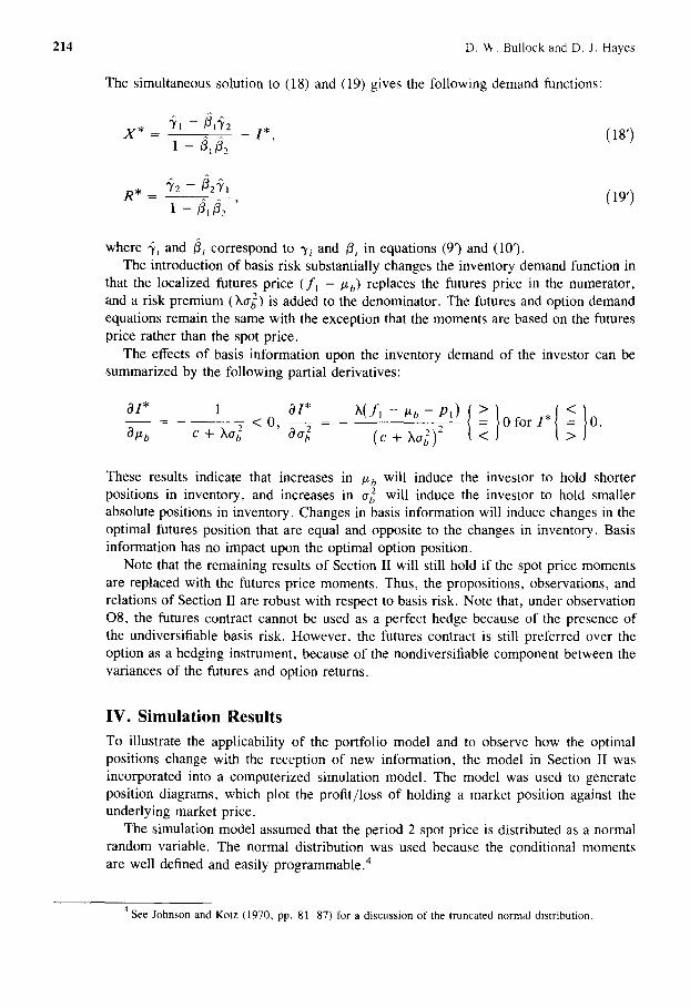
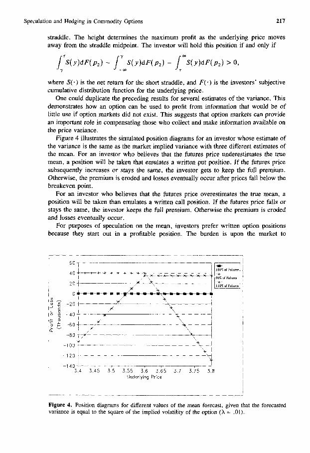
straddle. The height determines the maximum profit as the underlying price moves away from the straddle midpoint. The investor will hold this position if and only if

LrS(y)dF(p2) - f_~S(y)dF(p2) - L°°S(y)dF(P2) > O,

where S(.) is the net return for the short straddle, and F ( ' ) is the investors' subjective cumulative distribution function for the underlying price.

One could duplicate the preceding results for several estimates of the variance. This demonstrates how an option can be used to profit from information that would be of little use if option markets did not exist. This suggests that option markets can provide an important role in compensating those who collect and make information available on the price variance.

Figure 4 illustrates the simulated position diagrams for an investor whose estimate of the variance is the same as the market implied variance with three different estimates of the mean. For an investor who believes that the futures price underestimates the true mean, a position will be taken that emulates a written put position. I f the futures price subsequently increases or stays the same, the investor gets to keep the full premium. Otherwise, the premium is eroded and losses eventually occur after prices fall below the breakeven point.

For an investor who believes that the futures price overestimates the true mean, a position will be taken than emulates a written call position. I f the futures price falls or stays the same, the investor keeps the full premium. Otherwise the premium is eroded and losses eventually occur.

For purposes of speculation on the mean, investors prefer written option positions because they start out in a profitable position. The burden is upon the market to

60

40

20

0

~ -40

o ~ -60

-80 --~" /

-IOO

-12o

-140 3.4 3.45

" "x

\ : ~ ' +~\,

l~of ~ut urt*

\

"\"2t"

3.5 3.55 3.'6 3.65 3.'7 3.75 3.8 Underlying Price

Figure 4. Position diagrams for different values of the mean forecast, given that the forecasted variance is equal to the square of the implied volatility of the option (X = .01).


completely erode their initial gain (the premium) in order for a loss to be incurred. The size of the initial gain and the rate of erosion vary directly with the size of the combined futures and option position. Increases in the investor's estimate of the price variance or risk aversion will reduce the size of the optimal position.

Note that the profits and losses from the written option positions are substantially larger than for the straddle positions. Obviously, risk aversion is less of a factor for speculation on the mean than for speculation on the variance.

Note that these simulation results support, in general, the four basic observations of Wolf and Francis. However, for the case in which the investor regards the futures price to over- or underestimate the mean with a negative exponential utility function, Wolf and Francis show that the optimal position diagram will emulate a purchased put (for an overestimate) or a purchased call (for an underestimate). The simulation results in this study show that the investor will prefer a position that emulates a written call or put. This difference is probably due to model specification. In particular, the Wolf and Francis model contains multiple strike prices and both puts and calls. Also, the arbitrary specification of the VCV matrix in Wolf and Francis could account for the differences in position diagrams. Note, however, that the results of the model in this study are more in line with the common observation that speculators are primarily writers of options while hedgers are primarily purchasers of options.

V. Summary This study extends some recently published results by Wolf, and forthcoming results by Wolf and Francis, on how options and futures are used in constructing optimal portfolios. This extension allows us to determine how optimal positions respond to private and public information that modifies the investor's estimates of the mean and variance of the relevant future price distribution. The results indicate that investors will use futures contracts to hedge ownership of the underlying asset and to speculate on information changing the mean of the future price. They will use options to speculate on information changing the variance of the future price. These results are explained by showing that when investors can trade futures contracts, the option delta cannot be used to derive the optimal hedge ratio without adjusting for undiversifiable risk between options and futures. This undiversifiable risk is a result of the mapping of the terminal futures prices into a corresponding option price. This mapping is not one-to-one because a unique mapping of futures into option prices exists, but the opposite is not true. The theoretical results of this study are shown to be robust with respect to the degree of basis risk that exists in the market.

The theoretical demand equations for options and futures are used to simulate the impact of information changes relating to the mean and variance of future prices. The simulation results support and clarify the results derived from the maximization problem. In particular, investors will use positions that emulate straddles to speculate on the variance and will use positions that emulate written options to speculate on the mean.

A p p e n d i x A : D e r i v a t i o n o f t h e M e a n a n d V a r i a n c e o f P r o f i t s

Introducing a put option into an investor's portfolio results in a profit function that is nonsmooth where P2 = k. At points where P2 -< k, the profit function becomes

71" = (P2 P l ) " I - ' 2 -- -~CI + ( P 2 - - f , ) " X + (qi + k - p 2 ) "R.


At points where P2 > k, the profit function becomes

lr=(p2 P i ) ' I - ' 2 - 5 cI + ( P 2 - f , ) ' X + q , R "

Note that this function is continuous at P2 = k. To derive the mean and variance of profits, the following theorem is proven. This

theorem is a generalization of results discussed in Taylor and Karlin (1984, pp. 34-36), and in Beaumont (1986, pp. 207-209).

THEOREM. I f g(p) = gi (P) Vp <-- k, g(p) = g2(P) Vp > k, andp is a random variable with cumulative distribution function F(p), then

E [ g ( p ) ] = o t E [ g i ( p ) i p < k] + (1 - c0E [ g 2 ( p ) ] p > k],

var[ g ( p ) ] = c~ var[ g,(p) l p <_ k] + (1 - ot)var[ g,(P) I P > k]

+ o~(1 - , x ) {E [ g2(P) IP > k ] - E [ g,(P) I P -< k ] } ' ,

where

c~ = F ( k ) = p rob(p < k) .

Proof of (.4). Let

(A)

(s)

E [ g ( p ) ] = g i ( p ) d F ( p ) + g z ( p ) d F ( p ) . (A.1)

From the definition of conditional expectations, the following can be deduced:

= d F ( p ) . E [ g i ( p ) l p < k } , (A.2) - - o o

/( /( g z ( p ) d F ( p ) = dF(p ) " E[ g2(P) I P > k] . (A.3)

Substituting (A.2) and (A.3) into (A.I) and noting that / k ~ d F ( p ) = c~ and that [~ d F ( p ) = (1 - o0 gives the result in (A).

Proof o f (B). Let

g (p ) = l ( p < k ) g l ( p ) + l ( p > k )g2(p ), (A.4)

where l (y ) is the indicator function such that l (y ) = 1 if condition y is met and

220 D. W. Bullock and D. J. Hayes

l (y) = 0 otherwise. From the definition of variance, the following can be derived:

va r [g (p ) ] = E[g2(p)] - E 2 [ g ( p ) ] , (A.5)

E [g2 (p ) ] = E [ l ( p _ k)g2(p) + l ( p > k)g~(p)

+ 2 - l ( p _ < k ) l ( p > k)g,(p)g2(p)]

=olE[g2(p) l p ~ k ] + ( l - c~ )E[gZ(p ) lp>k] , (A.6)

E2[ g ( p ) ] = ~2 E2[ gl( P) l P <- k] + (1 - i f ) 2 E2[ g2(P) I P > k]

+2c~(1-c~)E[gl(p) lp<_k]E[g2(p)lp>k]. (A.7)

Substituting (A.6) and (A.7) into (A.5) and noting that

E[g2(p) ly] = var[gi(p) ly I + E2[gi(p) ly]

gives

var[ g ( p ) ] = c~ var[ g l (P ) l P <~ k] -k- (1 - a)var[ g2(P) l P > k]

+ ec(1-a){EZ[g, (p) lp< k] + E2[g2(P)[ P > k]}

-2ot(1-cQE[gl(p) l p < k ] E [ g z ( p ) l p > k ], (A.8)

which simplifies to the result in (B) since

E2[g1(P) IP<-k] +E2[gz(P) l p > k ]

= {El g2(P) IP > k] - E[ g,(P) IP <- k]}

+ 2" E[ g,(P) IP <- k]E[ g2(P) IP > k]. •

The authors wish to thank Jay Coggins, Mike Kehoe, and an anonymous reviewer for their helpful comments.

References Beaumont, G. P. 1986. Probability and Random Variables. Chichester, England: Ellis

Horwood Limited. Black, F. 1976. The pricing of commodity contracts. Journal of Financial Economics

3:167-179. Danthine, J. 1978. Information, futures prices, and stabilizing speculation. Journal of Eco-

nomic Theory 17:79-98. Holthausen, D. M. 1979. Hedging and the competitive firm under price uncertainty. American

Economic Review 69:989-995. Johnson, L. L. 1960. The theory of hedging and speculation in commodity futures. Review of

Economic Studies 27:139-151.


Johnson, N. L., and Kotz, S. 1970. Continuous Univariate Distributions- 1. Boston: Houghton Mifflin Co.

Labuszewski, J., and Sinquefield, J. 1985. Inside the Commodity Option Markets. New York: John Wiley and Sons.

Markowitz, H. 1952. Portfolio selection. Journal of Finance 7:77-91. McKinnon, R. I. 1967. Futures markets, buffer stocks, and income stability for primary

producers. Journal o f Political Economy 75:844-861. Smith, C. W., Jr. 1976. Options pricing: A review. Journal of Financial Economics 3:3-52. Stein, J. L. 1985. The Economics of Futures Markets. Englewood Cliffs, NJ: Prentice-Hall. Taylor, H., and Karlin, S. 1984. An Introduction to Stochastic Modeling. New York:

Academic Press. Tsiang, S. C. 1972. The rationale for the mean-standard deviation analysis, skewness preference,

and the demand for money. American Economic Review 62:354-371. Wolf, A. 1987. Optimal hedging with futures options. Journal of Economics and Business

39:141-158. Wolf, A., and Francis, J. C. 1991. Optimal portfolio choices of commodity options in incomplete

markets: A simulation analysis. In Advances in Quantitative Analysis of Finance and Accounting. VoL 1, Part A (Cheng F. Lee, ed.), Greenwich, CT: JAI Press, Inc., pp. 165-196.

Speculation and Hedging in Commodity Options: A Modification … · Speculation and Hedging in...

Documents

Transcript of Speculation and Hedging in Commodity Options: A Modification … · Speculation and Hedging in...