Spectrophotometric properties of dwarf planet Ceres from ... · Key words. minor planets,...

Astronomy & Astrophysics manuscript no. Ceres spectrophotmetry v2 referee c©ESO

2016

August 16, 2016

Spectrophotometric properties of dwarf planet

Ceres from VIR onboard Dawn mission

M. Ciarniello1, M. C. De Sanctis1, E. Ammannito2, A. Raponi1, A. Longobardo1,

E. Palomba1, F. G. Carrozzo1, F. Tosi1, J.-Y. Li3, S. Schroder4, F. Zambon1, A.

Frigeri1, S. Fonte1, M. Giardino1, C. M. Pieters5, C. A. Raymond6, C. T. Russell2

1 IAPS-INAF, via Fosso del Cavaliere, 100, 00133, Rome, Italy

2 University of California Los Angeles, Earth Planetary and Space Sciences,USA

3 Planetary Science Institute, USA

4 German Aerospace Center DLR, Institute of Planetary Research, Berlin, Germany

5 Department of Earth, Environmental, and PlanetarySciences, Brown University,

Providence, RI, USA

6 Jet Propulsion Laboratory, California Institute of Technology, Pasadena, USA

August 16, 2016

ABSTRACT

Aims. We present a study of the spectrophotometric properties of dwarf planet Ceres

in the VIS-IR spectral range by means of hyper-spectral images acquired by the VIR

imaging spectrometer onboard NASA Dawn mission.

Methods. Disk-resolved observations with phase angle within the 7.3◦ < α < 131◦ interval

have been used to characterize Ceres’ phase curve in the 0.465-4.05 µm spectral range.

Hapke’s model has been applied to perform the photometric correction of the dataset

to standard observation geometry at VIS-IR wavelength, allowing us to produce albedo

and color maps of the surface. The V band magnitude phase function of Ceres as been

computed from disk-resolved images and fitted with both the classical linear model and

HG formalism.

Results. The single scattering albedo and the asymmetry parameter at 0.55 µm are

respectively w = 0.14 ± 0.02 and ξ = −0.11 ± 0.08 (two lobes Henyey-Greenstein phase

function); at the same wavelength, Ceres’ geometric albedo as derived from our mod-

eling is 0.094 ± 0.007; the roughness parameter is θ = 29◦ ± 6◦. Albedo maps indicate

small variability at global scale with an average reflectance at standard geometry of

0.034±0.003. Nonetheless, isolated areas like the Occator bright spots, Haulani and Oxo

show an albedo much larger than the average. We measure a significant spectral phase

reddening and the average spectral slope of Ceres’ surface after photometric correction

Article number, page 1 of 31

arX

iv:1

608.

0464

3v1

[as

tro-

ph.E

P] 1

6 A

ug 2

016

Ciarniello et al.: Ceres’ spectrophotometric properties

is 1.1%kÅ−1 and 0.85%kÅ−1 at VIS and IR wavelengths, respectively. Broadband color

indices are V − R = 0.43 ± 0.01 and R − I = 0.34 ± 0.02. Color maps evidence that the

brightest features typically exhibit smaller slopes. The HG modeling of the V band

magnitude phase curve for α < 30◦ gives H = 3.14 ± 0.04 and G = 0.10 ± 0.04, while

the classical linear model provide V(1, 1, 0◦) = 3.48 ± 0.03 and β = 0.036 ± 0.002. The

comparison of our results with spectrophotometric properties of other minor bodies in-

dicate that Ceres has a less back-scattering phase function and a slightly larger albedo

than comets and C-type objects. However, the latter represents the closest match in

the usual asteroid taxonomy.

Key words. minor planets, asteroids: Ceres – methods: data analysis – techniques:

photometric – techniques: spectroscopic – techniques: imaging spectroscopy – planets

and satellites: surfaces

1. Introduction and rationale

After departing from asteroid Vesta in July 2012, the NASA Dawn spacecraft entered or-

bit around the dwarf planet Ceres on 6 March 2015. Prior to arrival, payload instruments

started acquiring remote sensing data of Ceres already from a distance of 1.2 × 106 km

on 1 December 2014 during the early Approach phase, making this body the first dwarf

planet and the thirteenth asteroid-like object to be imaged by a space-based mission, after

Gaspra (Helfenstein et al. 1994), Ida and Dactyl (Helfenstein et al. 1996) from Galileo

spacecraft; Mathilde (Clark et al. 1999) and Eros (Clark et al. 2002; Li et al. 2004) from

Near Shoemaker mission; Braille (Buratti et al. 2004) from Deep Space mission; Annefrank

(Hillier et al. 2011) from Stardust; Itokawa (Fujiwara et al. 2006) from Hayabusa; Steins

(Tosi et al. 2010; Spjuth et al. 2012) and Lutetia (Schroder et al. 2015; Longobardo et al.

2016) from Rosetta; Toutatis (Zou et al. 2014) from Chang’e 2; Vesta from DAWN (Li

et al. 2013b; Schroder et al. 2013; Longobardo et al. 2014). Ceres is the largest body in the

main asteroid belt, located at an average heliocentric distance of ≈ 2.77 AU, with a mass

of 9.38 × 1020 kg and an average radius of ≈ 470 km (Park et al. 2016). Interior models

based on shape data indicated that Ceres is a gravitationally relaxed and likely differenti-

ated object (Thomas et al. 2005; Castillo-Rogez & McCord 2010) with a rocky core and a

hydrated (icy or liquid) mantle (Neveu et al. 2015; Neveu & Desch 2015). Recent observa-

tions from Dawn and gravity data (Park et al. 2016) point instead to a high-density outer

shell dominated by rocky material (Castillo-Rogez et al. 2016). Spectral modeling of sur-

face spectra acquired by the Dawn mission evidences widespread presence of ammoniated

phyllosilicates (De Sanctis et al. 2015; Ammannito & et al. 2016) and abundant presence

of carbonate deposits in localized area due to aqueous alteration (De Sanctis et al. 2016)

as well as small spots of water ice in the northern hemisphere (Combe et al 2016).

The Dawn spacecraft (Russell & Raymond 2011) carries three instruments: the Framing



Camera (FC, Sierks et al. (2011)), the Visible and Infrared spectrometer (VIR, De Sanctis

et al. (2011) ) and the Gamma Ray and Neutron Detector (GRAND, Prettyman et al.

(2011)). VIR, whose dataset is investigated in this work, is an imaging spectrometer, work-

ing in the 0.2-5.1 µm spectral interval, using two channels covering the visible (VIS, 0.25-

1.05 µm) and infrared (IR, 1-5.1 µm) ranges, with a spectral sampling of 1.8 nm and 9.5

nm respectively and an instantaneous field of view (IFOV) of 250 µrad × 250 µrad. The

output of the instrument are hyper-spectral images (”cubes”), allowing one to characterize

the spatial and spectral distribution of the light reflected from the target as well as to mea-

sure its thermal emission by exploring the long wavelength range 4.5-5.1 µm (Tosi et al.

2014).

The study of the photometric properties of airless bodies by means of remote sensing ob-

servations at different wavelengths allows one to simultaneously investigate the physical

properties of their surface and composition. Furthermore, the derivation of a photometric

model from a set of observations of a given target permits to perform a photometric cor-

rection of the dataset itself (Li et al. 2015; Ciarniello et al. 2015), thus decoupling intrinsic

surface albedo variability from effects related to the observing geometry. To this twofold

aim we take advantage of VIR observations acquired from December 2014 up to June 2015

to study the global spectrophotometric properties of Ceres surface.

After a description of the dataset in Sec. 2, we describe the derivation of the photometric

correction of VIR observations by means of Hapke’s model (Hapke 2012) (Sec. 3), assessing

the average spectrophotometric properties of the surface. Photometrically corrected data

are then used to produce albedo maps and RGB color maps both in the VIS and in the

IR ranges (Sec. 4). Finally we compare the derived photometric properties of Ceres with

similar measurements reported in previous works and with the ones derived for other minor

bodies (asteroids and comets, Sec. 5) while a summary of the main findings of this paper

is in Sec. 6.

2. Dataset

VIR observations discussed in this study are from four different mission phases: Ceres

Approach (CSA), Rotational Characterization 3 (RC3), Ceres Transfer to Survey (CTS)

and Ceres Survey (CSS). Different mission phases are characterized by different spacecraft-

target distances (Fig. 1), progressively reducing from CSA (maximum altitude over the

surface 359006 km) to CSS (minimum altitude over the surface 4390 km). According to

this, the spatial resolution at ground varies from ≈90 km/pix to ≈1 km/pix as shown in Fig.

2. This dataset enables a proper characterization of Ceres’ spectrophotometric properties

at global scale, which is the focus of this work. For this reason, the High Altitude Mapping

Orbit (HAMO, distance 1450 km) and Low Altitude Mapping Orbit (LAMO, distance

735 km), which are characterized by a higher spatial resolution and complete the Dawn



mapping sequences, have not been analyzed in this study. Along with the spacecraft-target

distance, also the solar phase angle α varies across different observation sequences, covering

the overall 7.3◦ < α < 131◦ range (Fig. 1). The whole dataset investigated counts a total of

305 VIS-IR hyper-spectral images, corresponding to more than 3.6× 106 spectra, that have

been corrected for spectral artifacts (Carrozzo & et al 2016; Raponi 2015) and thermal

emission (Raponi et al. 2016). Given this, the available spectral range span from 0.465

µm to 4.05 µm, corresponding to the interval where high SNR is achieved. This prominent

dataset allows us to characterize a large fraction of Ceres surface (≈ 90%), and, providing

multiple observations of the different regions under different observation geometries, gives

us the possibility to constrain the photometric behavior of the surface.

01 Jan 2015

01 Feb 2015

03 Mar 2015

03 Apr 2015

03 May 2015

03 Jun 2015

CSA CSR CTS CSS

104

105

Dis

tance

[km

]

01 Jan 2015

01 Feb 2015

03 Mar 2015

03 Apr 2015

03 May 2015

03 Jun 2015

0

20

40

60

80

100

120

140

α [

deg

]

Fig. 1: Average target-spacecraft distance (solid line with triangles) and phase angle(dashed line with diamonds) for the VIR acquisitions investigated in this work. Each symbolcorresponds to one observations. The different orbit phases are indicated.

3. Photometric correction

The spectrophotometric output of a particulate medium in a remote sensing experiment

depends on the physical and compositional properties of the target as well as on the ob-

servation geometry, which is represented by the incidence i, emission e and phase α angles.

To compare images taken under different observation geometries, it is therefore necessary

to correct them for photometrical effects, in order to exploit the intrinsic variability re-

lated to the properties of the medium. This can be done by applying photometric models



Fig. 2: Ceres surface as observed by VIR. The three different images at 0.55 µm are takenduring RC3 (top panel, resolution of 3.4 km/pix), CTS (central panel, resolution of 1.3km/pix) and CSS (bottom panel, resolution of 1.1 km/pix) phases, respectively.

that describe the measured bidirectional reflectance r (or radiance factor I/F = πr) as a

function of i, e and g. Such photometric models can be either empirical (Minnaert 1941;

Akimov 1988) or semi-empirical (Longobardo et al. 2014) or physically based as in the case

of the Shkuratov et al. (1999) model and Hapke’s theory (Hapke 2012). The latter has been

widely used in spectrophotometric analysis of planetary objects, as shown in (Domingue

& Verbiscer 1997; Domingue et al. 2010; Ciarniello et al. 2011; Li et al. 2013a; Deau 2015;

Ciarniello et al. 2015) and in particular for asteroids (Clark et al. 1999, 2002; Domingue

et al. 2002; Li et al. 2004, 2006; Reddy et al. 2015). In this work we applied the Hapke’s

model to perform a photometric correction of VIR dataset following an approach similar

to Ciarniello et al. (2015) with three main differences:

– adoption of a two parameters Henyey-Greenstein single particle phase function (SPPF)

(Hapke 2012), instead of the single term expression (Henyey & Greenstein 1941)

– inclusion of the Shadow Hiding Opposition Effect (SHOE)



– inclusion of the multiple scattering term

Given this, the expression of the bidirectional reflectance we use to perform the photometric

correction is

r(i, e, α) =w

4πµ0e f f

µ0e f f + µe f f×

[BS H(α)p(α) + H(w, µ0e f f )H(w, µe f f ) − 1

]× S (i, e, α, θ), (1)

with:

– w: single scattering albedo (SSA)

– µ0e f f , µe f f : effective cosines of the incidence and emission angles, respectively

– BS H(α) =B0

1+1/h tan (α/2) : SHOE term depending on the opposition surge angular width h

and amplitude B0

– p(α) = 1+c2

1−b2

(1−2b cos(α)+α2)3/2 + 1−c2

1−b2

(1+2b cos(α)+α2)3/2 : two parameters SPPF; b ranges in the [0; 1)

interval and represents the width of the SPPF back-scattering and forward-scatterings

lobes; c determines the SPPF behavior: back-scattering (> 0) or forward-scattering

(< 0)

– H(w, x): Chandrasekhar’s function (Chandrasekhar 1960), accounting for the multiple

scattering contribution

– S (i, e, α, θ): shadowing function

– θ: surface average slope parameter

With respect to the complete version of the Hapke’s model, this expression does not include

the Coherent Backscattering Opposition Effect (CBOE) (Hapke 2002) and doesn’t take

into account for the effects of porosity described in Hapke (2008); Ciarniello et al. (2014).

This is justified by the fact that CBOE is significant at very small phase angles (< 2◦),

outside the range investigated in this work, while, as discussed in (Li et al. 2013a; Ciarniello

et al. 2015), the effect of porosity cannot be decoupled by SSA for low albedo objects as

Ceres. According to this, the free parameters in the model are w, b, v, B0, h, all depending

on the wavelength, and θ, which, being related to surface morphology, has no spectral

dependence. Since the smallest investigated phase angle is 7◦, it is not possible to model

the opposition surge and constrain SHOE parameters B0, h. We then assume the values

reported by Helfenstein & Veverka (1989) across the whole investigated spectral range,

B0 = 1.6 and h = 0.06 .

The whole dataset used to derive the photometric correction, at 0.55 µm wavelength, is

shown in Fig. 3, where I/F is reported as a function of the phase angle. Pixels acquired with

large incidence and emission angle (i, e > 70◦) and very low signal (I/F < 0.001 at 0.55 µm)

have been filtered out. This allows us to minimize the effect due to unfavorable geometries,

that can be affected by relatively larger errors, and limit the occurrence of pixels in total

or partial shadow.



0 20 40 60 80 100 120 140α [deg]

0.00

0.02

0.04

0.06

0.08

0.10

I/F

Normalized root pixel density

0.00 0.25 0.50 0.75 1.00

Fig. 3: I/F at 0.55 µm as a function of the phase angle: contour plot showing the squareroot of points density normalized to its maximum value.

The algorithm used to derive the set of Hapke’s parameters for Ceres dataset is similar

to the one adopted in Ciarniello et al. (2015), but presents some significative diversities, so

we consider useful to report the main steps here:

– The I/F at a given wavelength of each pixel is multiplied by the factor 4 µ0e f f +µe f f

µ0e f f S (i,e,α,θ0) ,

where θ0 is a given value of the roughness slope parameter. Assuming eq. 1, this quantity,

that we call here equigonal albedo Aeq (Fig. 4) in analogy with Akimov’s photometric

model (Shkuratov et al. 1999), corresponds to the following expression:

Aeq(α, i, g) = w[BS H(α)p(α) + H(w, µ0e f f )H(w, µe f f ) − 1

]1

– the equigonal albedo is averaged on phase angle bins of 1◦ obtaining 〈Aeq〉α (Fig. 4)

– 〈Aeq〉α is then fitted with its corresponding averaged expression from Hapke theory

w〈BS H p〉α +w〈H(w, µ0e f f )H(w, µe f f )−1〉α, which depends on the photometric parameters

of the model and is computed on the observation geometries of the investigated dataset

– the output of this algorithm is a set of photometric parameters at each wavelength for

the given θ0: this is repeated by varying θ in the range [0◦; 60◦) at steps of 1◦ (Fig. 5)

– the whole dataset is photometrically corrected using separately all the derived sets of

parameters (characterized by different values of θ). This is done by computing the pho-

tometrically corrected radiance factor I/Fstd, which is the measured I/F(i, e, α) reported

to standard geometry (i = 30◦, e = 0◦, α = 30◦) by means of the following relation:

I/Fstd =I/F(i, e, α)

I/Fm(i, e, α)I/Fm(30◦, 0, 30◦) (2)

where the subscript m indicates the modeled radiance factor

1 Equigonal albedo in Akimov’s theory doesn’t depend on i and e. Conversely, our definitionformally depends on incidence and emission angle through the the Chandrasekhar’s function.However, in the case low albedo surfaces as Ceres’, H(w, x) ≈ 1 and the dependence on i and e isweak.



– the final set of parameters is defined as the one that minimizes, at selected wavelengths

(see Sec. 3.1), the residual correlation of I/Fstd with the observation geometry, i. e. with

the incidence, emission and phase angles.

0 20 40 60 80 100 120 140α [deg]

0.0

0.1

0.2

0.3

0.4

0.5

0.6

Aeq


0.00 0.25 0.50 0.75 1.00

Fig. 4: Aeq at 0.55 µm as a function of the phase angle for θ0 = 0◦: contour plot showing thesquare root of points density normalized to its maximum value. Blue diamonds representsthe average equigonal albedo on 1◦ phase angle bins 〈Aeq〉α.

0 20 40 60 80 100 120 140α [deg]

0.0

0.1

0.2

0.3

0.4

0.5

0.6

Aeq

θ [deg]

0 15 30 45 60

Fig. 5: Average Aeq at 0.55 µm as a function of the phase angle for different θ. The incrementof θ produces an enlargement of Aeq at large phase angles with respect to small ones as wellas a slight increase of its overall level.

3.1. Surface roughness

The final surface roughness parameter is determined as the one that provides the minimal

residual correlation of the corrected I/F with incidence, emission and phase angles. As

stated above, this parameter is assumed to have no spectral dependence, being related



to terrain morphology at scales much larger than the wavelength (Hapke 2012) and it

is constrained using information from selected wavelengths in the VIS (0.545µm ≤ λ ≤0.946µm) and in the IR (1.02µm ≤ λ ≤ 2.99µm), characterized by good SNR and poorly

affected by residual thermal emission. For a given θ0 and the corresponding set of spectral

parameters we computed the corrected reflectance I/Fstd and performed averages on 1◦ bins

of incidence, emission and phase angles, respectively, producing a set of three curves at each

wavelength: 〈I/Fstd〉i, 〈I/Fstd〉e and 〈I/Fstd〉α. These quantities are then normalized at the

smallest incidence, emission and phase angle, respectively and spectrally averaged, thus

producing a final set for each value of θ, that, for brevity, we refer as Ci, Ce and Cα (Fig.

7). These curves quantify the residual correlation of the corrected I/F with observation

geometry for a given value of the slope parameter. Each set of Ci, Ce and Cα, is fitted

with a line with null angular coefficient (it represents the ideal behavior in case of no

residual correlation) and the resulting residuals of the three fits are summed to produce a

χ2 variable, whose distribution as a function of the slope parameter is reported in Fig. 6.

The final value of θ is chosen as the one producing the smallest χ2 obtaining θ = 29◦ ± 6◦.

This value is much lower than the one derived in (Li et al. 2006) θ = 44◦ from HST data.

This difference can be explained by the fact that in Li et al. (2006) a much smaller range

of phase angles was explored (6.1◦ − 6.2◦), thus not allowing a thorough constraining of the

effect of surface roughness, which is increasingly important at large α. Another possible

cause for the large value of θ derived in Li et al. (2006) is that the point spread function of

the High Resolution Channel of the Advanced Camera for Surveys on HST, used to perform

Ceres observations, was few pixels wide, with the target being roughly 30 pixels across. This

could produce a larger reduction of the signal towards the edge of Ceres’ disk, resulting in

a higher roughness parameter (J.-Y. Li, personal communication). Recent evaluations of

the roughness parameter from DAWN-FC observations report θ = 20◦ ±3◦ (Li et al. 2016b)

and θ = 22◦ ± 2◦ (Schroder & et al. 2016). Our estimate of θ, albeit fairly larger than Li

et al. (2016b) and Schroder & et al. (2016) results, is still compatible with their values

within the error .

3.2. SSA

In Fig. 8 the derived single scattering albedo is shown as a function of wavelength. This

quantity can be considered as representative of the average spectral properties of the surface

of Ceres and it is linked to its composition. In the VIS range the SSA spectrum has a sharp

absorption at the shortest wavelength with a moderate red slope from 0.47 µm up to 0.9 µm.

The spectrum in the IR has a slightly positive slope from 1 µm up to 2.65 µm. Absorption

features at 2.7 µm and 3.06 µm, attributed to -OH and -NH4 bearing minerals, as well

as carbonates bands at 3.3 µm and 3.95 µm can be recognized (De Sanctis et al. 2015).

The value of the SSA 0.55 µm is w = 0.14 ± 0.02 (the dispersion is related to the error



0 10 20 30 40 50 60 70e [deg]

0.8

0.9

1.0

1.1

1.2

Ci

(a)

0 10 20 30 40 50 60 70e [deg]

0.8

0.9

1.0

1.1

1.2

Ce

(b)

0 20 40 60 80 100 120 140α [deg]

0.6

0.7

0.8

0.9

1.0

1.1

1.2

Cα

(c)

Fig. 6: Ci (top panel), Ce (central panel) and Cα (bottom panel). In each plot we show twocurves for comparison, corresponding respectively to θ0 = 0◦ (solid line) and θ0 = 29◦ (dot-dashed line). It can be noted that increasing the slope parameter allows to compensate forthe reduction of signal at large i (≈ 10%)and e (≈ 5%) while minimizing the amplitude ofthe modulation of the signal at large α for Cα. A residual modulation of Cα with the phaseangle is still present for θ0 = 29◦ possibly due to the fact that regions with intrinsicallydifferent albedo have been observed at different phase angles or to a deviation of the regolithSPPF behavior from the adopted Henyey-Greenstein formulation. Smaller residuals (< 3%)can be also noted for Ci and Ce.

on θ parameter),which is much larger with respect to the one provided by Helfenstein &

Veverka (1989) (w = 0.06) and Li et al. (2006) (w = 0.07) and different from the ones



0 10 20 30 40θ [deg]

1.0

1.2

1.4

1.6

1.8

2.0

2.2

2.4N

orm

aliz

ed χ

2

Fig. 7: χ2 normalized at its maximum value as a function of the slope parameter.

derived for the various models described in Reddy et al. (2015) (w = 0.070, 0.11, 0.083) and

Li et al. (2016b) (w = 0.094 − 0.11). It is important to mention that Helfenstein & Veverka

(1989); Li et al. (2006); Reddy et al. (2015) analysis have been conducted on ground-based

data, while Li et al. (2016b) used Dawn-FC observations in the 30◦ −90◦ phase angle range

(effective wavelength 730 nm). All these works assume a single parameter expression for

the SPPF, given the relatively limited investigated phase angle range. The adoption of

different versions of the Hapke’s model and the possibility to access a much larger portion

of the phase curve with VIR data can account for the differences in the retrieved SSAs.

3.3. SPPF and cosine asymmetry factor

As described in sec. 3 the single particle phase function depends on two parameters, b

and v, which determine the shape of the SPPF and its behavior as a function of the phase

angle. These quantities can be combined in a single expression to give the cosine asymmetry

factor ξ = −bv = −〈cos(α)〉. It represents the opposite of the average value of the phase angle

cosine weighted by the SPPF. Negative values of ξ imply a a predominantly backscattering

single particle phase function, that turns to forward-scattering for a positive asymmetry

factor. A value of ξ = 0 indicate a symmetric SPPF. In Fig. 9 the spectral dependence of ξ

is shown, as obtained from the derived values of b and v. It can be noted that the behavior

of the SPPF changes from backscattering at short wavelength to fairly symmetric in the

IR, being partially correlated with the SSA. The value of the asymmetry factor at 0.55 µm

is ξ = −0.11 ± 0.08. The large dispersion associated to this quantity is related to the error

on the roughness parameter θ, and is due to the coupling among the different terms of the

Hapke’s model and in particular between the SPPF and the shadowing function S (i, e, α, θ).



1 2 3 4wavelength [µm]

0.00

0.05

0.10

0.15

0.20

0.25

0.30w

Fig. 8: SSA spectrum: missing parts correspond to the order sorting filters positions andthe VIS-IR channels junction.

1 2 3 4wavelength [µm]

-0.20

-0.15

-0.10

-0.05

0.00

0.05

0.10

ξ

Fig. 9: ξ as a function of wavelength: missing parts correspond to the order sorting filterspositions and the VIS-IR channels junction.



3.4. Spectral slopes and phase reddening

The dependence of the SPPF on wavelength implies that the spectral output depends on

phase angle. This is shown in Fig. 10, where the spectral slope in the VIS (0.55-0.80 µm) and

IR (1.2-2 µm) ranges as derived by VIR observations are reported as a function of α. These

quantities are defined as S VIS =I/F0.80µm−I/F0.55µm

I/F0.55µm(8kÅ−5.5kÅ)and S IR =

I/F2µm−I/F1.2µm

I/F1.2µm(20kÅ−12kÅ)respectively.

0 20 40 60 80 100 120 140α [deg]

-0.2

-0.1

0.0

0.1

0.2

SV

IS

SVIS = 4.6E-04α - 2.2E-03


0.00 0.25 0.50 0.75 1.00

(a)

0 20 40 60 80 100 120 140α [deg]

-0.06-0.04

-0.02

0.00

0.02

0.04

0.06

0.08

SIR

SIR = 1.5E-04α + 4.3E-03


0.00 0.25 0.50 0.75 1.00

(b)

0 20 40 60 80 100 120 140α [deg]

-0.2

-0.1

0.0

0.1

0.2

SV

IS

SVIS = -9.4E-07α + 1.1E-02


0.00 0.25 0.50 0.75 1.00

(c)

0 20 40 60 80 100 120 140α [deg]

-0.06-0.04

-0.02

0.00

0.02

0.04

0.06

0.08

SIR

SIR = -4.6E-07α + 8.5E-03


0.00 0.25 0.50 0.75 1.00

(d)

Fig. 10: Density plot of S VIS (a) and S IR (b) as a function of α. The same quantities afterphotometric correction are reported in panels (c) and (d). Linear fits to the distributionsare reported as black solid lines in the plots, with their equations: the angular coefficientis expressed in [kÅ−1deg−1] and intercept in [kÅ−1].

Both S VIS and S IR show a positive fairly linear correlation with phase angle (Fig.

10a,10b), similarly to what is observed by Li et al. (2016b), with an increment of 4.6 ×10−2%kÅ−1deg−1 in the VIS and 1.5 × 10−2%kÅ−1deg−1 in the IR, which is removed after

the photometric correction (Fig. 10c,10d) giving S VIS = 1.1%kÅ−1 and S IR = 0.85%kÅ−1.

This behavior, indicated as ”phase reddening”, is common for asteroids (see Li et al. (2015)

and references therein) and airless bodies in general: comets (Ciarniello et al. 2015), icy

satellites (Cuzzi et al. 2002; Ciarniello et al. 2011; Filacchione et al. 2012) and planetary

rings (Filacchione et al. 2014; Ciarniello et al. 2016). Moreover it has been observed in

lab measurements and light scattering simulations from Schroder et al. (2014). From these

studies it emerges that two typical behaviors of the spectral slopes with phase angle can

be recognized: arch-shaped (Schroder et al. 2014) and monotonic. The first, associated to

semi-transparent and relatively bright particles is explained by the combined effect of mul-

tiple scattering and surface shadowing (Kaydash et al. 2010), while the second is shown by

opaque and low albedo ones and possibly related to particle surface roughness. The latter is

in good agreement with the monotonic phase reddening measured by VIR at Ceres, which



is characterized by a dark surface.

3.5. Photometric correction accuracy

The derived set of photometric parameters is used in Eq. 2 to report the measured I/F(i, e, α)

to its correspondent value in standard observation geometry I/Fstd. This implies the as-

sumption that surface photometric behavior is globally uniform, and that changes in I/Fstd

are due to the variability of the intrinsic albedo properties of the different observed regions.

As shown below this approximation is reasonable in the case of Ceres’ surface, which shows

small variability at large scale (>1 km). Nonetheless a number of isolated bright features

have been recognized throughout the surface of the body, as also reported by Schroder &

et al. (2016); De Sanctis et al. (2016); Russell et al (2016) showing a much larger albedo

than the average, that cannot be described by the same set of photometric parameters

derived here. In those cases, the value of the I/Fstd is an approximated estimate of the real

reflectance of the surface as observed in standard geometry.

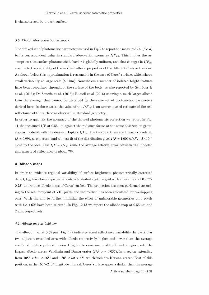
In order to quantify the accuracy of the derived photometric correction we report in Fig.

11 the measured I/F at 0.55 µm against the radiance factor at the same observation geom-

etry as modeled with the derived Hapke’s I/Fm. The two quantities are linearly correlated

(R = 0.99), as expected, and a linear fit of the distribution gives I/F = 1.006× I/Fm−5×10−4

close to the ideal case I/F = I/Fm while the average relative error between the modeled

and measured reflectance is about 7%.

4. Albedo maps

In order to evidence regional variability of surface brightness, photometrically corrected

data I/Fstd have been reprojected onto a latitude-longitude grid with a resolution of 0.25◦×0.25◦ to produce albedo maps of Ceres’ surface. The projection has been performed accord-

ing to the real footprint of VIR pixels and the median has been calculated for overlapping

ones. With the aim to further minimize the effect of unfavorable geometries only pixels

with i, e < 60◦ have been selected. In Fig. 12,13 we report the albedo map at 0.55 µm and

2 µm, respectively.

4.1. Albedo map at 0.55 µm

The albedo map at 0.55 µm (Fig. 12) indicates zonal reflectance variability. In particular

two adjacent extended area with albedo respectively higher and lower than the average

are found in the equatorial region. Brighter terrains surround the Planitia region, with the

largest albedo across Vendimia and Dantu crater (I/Fstd ≈ 0.037), in a region extending

from 105◦ < lon < 165◦ and −30◦ < lat < 45◦ which includes Kerwan crater. East of this

position, in the 165◦−210◦ longitude interval, Ceres’ surface appears darker than the average



0.00 0.02 0.04 0.06 0.08I/Fm

0.00

0.02

0.04

0.06

0.08

I/F


0.00 0.25 0.50 0.75 1.00

Fig. 11: I/F against I/Fm at 0.55 µm: the black solid line is the linear fit to the distributionwith equation I/F = 1.006 × I/Fm − 5 × 10−4.

with I/Fstd ≈ 0.033. The rest of the surface with −30◦ < lat < 30◦ exhibits intermediate

albedo I/F ≈ 0.034. Isolated features corresponding to morphological structures can be

recognized, as the Haulani (lon ≈ 11◦, lat ≈ 6◦, max I/Fstd = 0.050) and Oxo (lon ≈ 0◦,

lat ≈ 42◦ max I/Fstd = 0.068) craters, the region in correspondence of Juling and Kupalo

(max I/F ≈ 0.057) and the Liberalia Mons area (I/Fstd = 0.041). Bright spots in Occator

crater are not fully resolved due to the limited spatial resolution of the dataset. In fact,

this region has been observed mainly during RC3 phase with a typical resolution of 3.4

km obtaining a maximum value of I/Fstd = 0.12, whereas De Sanctis et al. (2016) report

0.26 from HAMO data. On the North-East hand of the crater a portion characterized by

low reflectance (I/Fstd ≈ 0.031) can be noticed. In this case the transition from high to low

albedo is very sharp, and it is distributed along a linear feature extending from lon ≈ 232◦,

lat ≈ 32◦ to lon ≈ 252◦, lat ≈ 14◦. Two distinct darker areas with respect to the nearby

terrains are located in correspondence of Urvara and Yalode craters with I/Fstd ≈ 0.032.

Albedo level tends to increase towards the poles, possibly due to overcorrection of the

reflectance level because of unfavorable observation geometries (large i and e). It is worth

mentioning that the albedo distribution derived in this work is in good agreement with the

one derived in Li et al. (2006) from HST images and the one obtained with observation

from the Dawn Framing Camera (Schroder & et al. 2016).



Fig. 12: Albedo map at 0.55 µm.



4.2. Albedo map at 2 µm

The albedo map at 2 µm (Fig. 13) appears fairly similar to the one derived at 0.55 µm

but presenting some peculiar differences. While albedo variability is preserved at large

scale with minor modifications (see for example the shape of the bright region located at

105◦ < lon < 165◦ and −30◦ < lat < 45◦), isolated structures in the VIS not always show

an IR counterpart. The most significative example is the Haulani crater, characterized by

dark ejecta at 2 µm, showing an increase of brightness in the central part. This indicates

that along with albedo variation also spectral variegation occurs. In order to isolate regions

with maximum spectral variability we report in Fig. 14 the relative difference of the two

maps, computed according to the following equation:

∆ = 2I/Fstd(2µm) − I/Fstd(0.55µm)I/Fstd(0.55µm) + I/Fstd(2µm)

(3)

Beside Haulani also Occator’s floor exhibits negative values of ∆, indicating different

spectral properties with the rest of the surface. Also bright spots inside Occator show vari-

ability of the ∆ parameter, with adjacent positive and negative values. Although De Sanctis

et al. (2016) reported that these regions are rich in carbonates, the sharp variation of ∆

shown here, given the limited extension of the spots, is more likely due to a slight displace-

ment between the VIS and IR reprojected pixels than to compositional variability. Finally,

Oxo crater and a relatively larger region associated to Juling and Kupalo craters exhibit a

negative ∆ as well. All these areas, with the exception of Occator floor are characterized by

large albedo in the VIS range, suggesting that small-scale high albedo features are charac-

terized by a bluish spectrum. This is confirmed from the enhanced colors maps shown in

sec. 4.4.

4.3. Albedo variability

In Fig. 15 histograms for I/Fstd at 0.55 µm and 2 µm as derived from the corresponding

albedo maps are shown. The distribution is unimodal in both cases, with average values

of 0.034 ± 0.003 at 0.55 µm and 0.032 ± 0.002 at 2 µm. This indicates that on global

scale Ceres’ surface, as observed at VIR resolution, is fairly uniform. The width of the

distributions of Fig. 15 is linked to the intrinsic albedo variability at the surface, to the

error on the measured reflectance and to the error associated to the photometric correction

(uncertainties on observation geometry and photometric parameters). It is then possible

to give an upper limit of the global albedo variability, being of the order of 9% in the VIS

and 6% in the IR. On the other hand, at local scale, albedo variability can be much larger,

as in the case of the brightest features like Occator bright spots, Oxo and Haulani, which

correspond to areas with limited extension.



Fig. 13: Albedo map at 2 µm.



Fig. 14: Map of the albedo difference at 2 µm and 0.55 µm.



0.020 0.025 0.030 0.035 0.040 0.045 0.050

I/Fstd

0.00

0.02

0.04

0.06

0.08

0.10

0.12

0.14

Su

rface f

racti

on

<I/Fstd

> = 0.034

σ = 0.003

(a)

0.020 0.025 0.030 0.035 0.040 0.045 0.050

I/Fstd

0.00

0.02

0.04

0.06

0.08

0.10

0.12

0.14

Su

rface f

racti

on

<I/Fstd

> = 0.032

σ = 0.002

(b)

Fig. 15: Histograms of I/Fstd at 0.55 µm (a) and 2 µm (b): the average values 〈I/Fstd〉 andthe standard deviation σ of the distributions are indicated. Histograms are built accordingto the real area subtended by each pixel in the maps.

4.4. RGB maps

In Fig. 16 an enhanced color map of Ceres’ surface in the VIS is shown. A large fraction

of the surface exhibits a reddish spectrum, with bluish features nearby small high albedo

regions as Haulani, Occator, Oxo and the Juling-Kupalo area. Conversely, the relatively

bright region between Dantu and Vendimia appears redder with respect to the darker

Planitia. From Haulani an elongated bluish region extends up to Ikapati. This confirms the

color distribution shown in the VIS range by Nathues et al. (2015) and Schroder & et al.

(2016). A similar enhanced color distribution is obtained at IR wavelengths (Red=2.2 µm,

Green=1.8 µm, Blue=1.2µm, Fig. 17). The main differences with respect to the VIS range

are found in the brighter terrains around the Planitia, which appear bluish in the IR, and

on the North-East side of Occator, showing a reddish spectrum when compared to the blue

material surrounding the crater on the South-West part.

5. Comparison with other minor bodies

Prior to Dawn mission to Vesta and Ceres, several minor bodies, including asteroids and

comets have been closely imaged by remote sensing instruments onboard space missions.

The observation of these objects under viewing geometries that are not accessible from

ground-based facilities enabled comparison of their photometric curves on the basis of

their shape (Longobardo et al. 2016) or Hapke’s parameters. In Table 1 we report the

Hapke’s parameters at visible-infrared wavelengths for a set of asteroids and comets and

from previous Ceres’ studies, as compared to the ones derived in this work.



Fig. 16: RGB (Red=0.700 µm, Green=0.550 µm, Blue=0.465 µm) map in the VIS range.



Fig. 17: RGB (Red=2.2 µm, Green=1.8 µm, Blue=1.2 µm) map in the IR range.



5.1. Ceres

The value of the SSA albedo at 0.55 µm derived from VIR data is much larger with respect

to previous measurements by Li et al. (2006), while it is closer to the determination given

by Reddy et al. (2015) and Li et al. (2016b). The large difference with Li et al. (2006)

result can be explained by the different shapes of the SPPF adopted in this work (two

terms against single term expression) and the limited phase angle range investigated in Li

et al. (2006). Substantial differences are found also in the derivation of the ξ parameter,

leading to a more symmetric shape (less back-scattering) of the SPPF if compared to the

result of Li et al. (2006), Reddy et al. (2015) and Li et al. (2016b). Again, this can be due

to the reasons explained above along with the effect of a possible degeneration of Hapke’s

model parameters (Li et al. 2015): in particular, a more back-scattering SPPF can be

compensated by a reduction of the SSA if the investigated phase angle range is not large

enough. A similar explanation can be valid also for the different values of the roughness

parameter, which in this work gives θ = 29◦ while it is estimated equal to 44◦ in Li et al.

(2006) and 20◦ in Li et al. (2016b).

5.2. Other minor bodies

The comparison with Hapke’s parameters derived for other minor bodies indicates that

Ceres’ SSA is intermediate between the dark comets and C-type Mathilde, and the brighter

S-type asteroids, while the asymmetry parameter is the largest of the whole dataset. We

remind here that the large majority of Hapke models reported in Table 1 is performed with

a single term Henyey-Greenstein SPPF limiting the significance of the comparison on ξ.

The roughness parameter value is among the largest of the distribution, possibly indicating

significant sub-pixel (< 1 km scale ) roughness. Because of the coupling between Hapke’s

parameter and their possible degeneration, a more thorough comparison of the photometric

properties of different bodies can be performed confronting quantities that are combinations

of the modeled parameters. In this perspective the geometric albedo Ageo and integral phase

function Φp(α) (Hapke 2012) can give clues on the intrinsic surface albedo properties and the

scattering behavior with phase angle. From our modeling we derive Ageo = 0.094±0.007 that

is in excellent agreement with previous measurements by Reddy et al. (2015) and Li et al.

(2006) (Table 1) and the recent determination by Li et al. (2016a) reporting 0.085± 0.005.

This indicates that Ceres has the darkest surface among the asteroids reported here, with

the exception of Mathilde, whose geometric albedo is comparable to the ones derived for

comets. When compared to the average geometric albedo of the different asteroids classes,

the one for C-type objects represents the closest match (see Table 2). This is also shown in

Fig. 18 where the modeled full-disk reflectance FDR(α), defined as FDR(α) = Ageo ×Φp(α),

is reported for all the objects of Table 1: Ceres’ curve is positioned above the FDR of

comets and C-type Mathilde. In Fig. 19 the integral phase function is shown. In this case



Table 1: Ceres’ Hapke parameters and geometric albedo compared to asteroids andcometary nuclei.

Target S S A ξ B0 h θ Ageo phase angle coverage Asteroid type(1)Ceres (this work) 0.14 ± 0.02 −0.11 ± 0.08 (1.6) (0.06) 29◦ ± 6◦ 0.094 ± 0.007 7.3◦ − 131◦ -

(1)Ceresa 0.094 − 0.11 −0.35 ± 0.05 - - 20◦ ± 3◦ 0.085 ± 0.005 30◦ − 90◦ -

(1)Ceresb 0.070 ± 0.002 (−0.4) (1.6) (0.06) 44◦ ± 5◦ 0.087 ± 0.003 6.1◦ − 6.2◦ -(1)Ceresc 0.11 −0.29 (1.6) (0.06) (44◦) 0.094 0.9◦ − 21.4◦ -

(253)Mathilded 0.035 ± 0.006 -0.25 ± 0.04 3.2 ± 1.0 0.074 ± 0.003 19◦ ± 5◦ 0.047 ± 0.005 40◦ − 138◦ C(4)Vestae 0.500 -0.229 1.7 0.07 17.7◦ 0.38 ± 0.04 7.7◦ − 80◦ V

(21)Lutetiaf 0.25 -0.22 1.58 0.052 24◦ - 0◦ − 136.4◦ M(21)Lutetiag 0.226 ± 0.002 −0.28 ± 0.02 1.79 ± 0.08 0.041 ± 0.003 28◦ ± 1◦ 0.194 ± 0.002 0.15◦ − 156◦ M

(2867)Steinsh 0.57 ± 0.05 −0.27 ± 0.01 0.60 ± 0.01 0.062 ± 0.020 28◦ ± 2◦ 0.39 ± 0.02 0.36◦ − 141◦ E(951)Gasprai 0.36 ± 0.07 −0.18 ± 0.04 1.63 ± 0.07 0.06 ± 0.01 29◦ ± 2◦ 0.22 ± 0.06 2◦ − 51◦ S

(243)Idaj 0.218+0.024−0.005 −0.33 ± 0.01 1.53 ± 0.01 0.02 ± 0.005 18◦ ± 2◦ 0.206 ± 0.032 0.6◦ − 109.8◦ S

Dactylj 0.211+0.028−0.010 −0.33 ± 0.03 (1.53) (0.02) 23◦ ± 5◦ 0.198 ± 0.050 19.5◦ − 47.6◦ S

(433)Erosk 0.33 ± 0.03 −0.25 ± 0.02 1.4 ± 0.1 0.01 ± 0.004 28◦ ± 3◦ 0.23 0.3◦ − 110◦ S

(25143)Itokawal 0.36 ± 0.05 −0.5 ± 0.1 (1.0) (0.022) (20◦) 0.53 ± 0.04 27◦ − 87◦ S(25143)Itokawam 0.42 ± 0.02 −0.35 ± 0.01 0.87 ± 0.02 0.01 ± 0.001 26◦ ± 1◦ 0.33 0.2◦ − 38.4◦ S(5535)Annefrankn 0.41 ± 0.05 −0.19 ± 0.03 (1.32) 0.046 ± 0.013 (20◦) 0.232 ± 0.038 2.3◦ − 90◦ S

67P/Churyumov-Gerasimenkoo 0.052 ± 0.013 −0.42 − − 19◦+4−9 0.062 ± 0.002 1.2◦ − 111.5◦ -

67P/Churyumov-Gerasimenkop 0.037 ± 0.002 −0.42 ± 0.03 1.95 ± 0.12 0.023 ± 0.004 15◦ 0.0589 ± 0.0034 1.3◦ − 53.9◦ -19P/Borrellyq 0.057 ± 0.009 −0.43 ± 0.07 1.0 0.039 22◦ ± 5◦ 0.072 ± 0.020 51◦ − 75◦ -

103P/Hartley 2r 0.036 ± 0.006 −0.46 ± 0.06 (1.0) (0.01) 15◦ ± 10◦ 0.045 ± 0.009 79◦ − 93◦ -9P/Tempel1s 0.039 ± 0.005 −0.49 ± 0.02 (1.0) (0.01) 16◦ ± 8◦ 0.051 ± 0.009 63◦ − 117◦ -81P/Wild 2t 0.038 ± 0.04 −0.52 ± 0.04 (1.0) (0.1) 27◦ ± 5◦ 0.059 ± 0.004 11◦ − 100◦ -

Notes. (a) Li et al. (2016b), clear filter centered at 730 nm, geometric albedo by Li et al. (2016a).(b) Li et al. (2006)(c) Reddy et al. (2015), case 2(d) Clark et al. (1999), at 0.7 µm. NEAR data have been combined with telescopic observations atphase angles from 1◦ to 16◦(e) Li et al. (2013b)(f) Raponi (2015), average values in the 1.1 µm - 2.4 µm wavelength range. These quantities arederived by applying Hapke (2012) model, including the effect of porosity with K=1.18.(g) Masoumzadeh et al. (2015), at 631.6 nm and 649.2 nm.(h) Spjuth et al. (2012) at 630 nm. These quantities are derived by applying Hapke (2012) model,including the effect of porosity with K=1.24.(i) Helfenstein et al. (1994) at 0.56 µm. Values are derived from Earth-based and Galileo missioncombined data.(j) Helfenstein et al. (1996) at 0.55 µm. For Ida, values are derived from Earth-based and Galileomission combined data.(k) Li et al. (2004), at 0.55 µm. Near data have been combined with telescopic observations atphase angles below 53◦.(l) Lederer et al. (2005): ground based observations in the V band, solution 4.(m) Kitazato et al. (2008), at 1.57 µm. Geometric albedo was not reported in the original paperand has been here computed from Hapke’s parameters.(n) Hillier et al. (2011), at 630 nm. Stardust data have been combined with telescopic observationsat phase angles from 2.3◦ to 18.3◦.(o) Ciarniello et al. (2015).(p) Fornasier et al. (2015).(q) Li et al. (2007b), R band.(r) Li et al. (2013a). DIXI observations have been combined with Gemini and HST data at lowphase angles.(s) Li et al. (2007a).(t) Li et al. (2009), R band.

the phase curves can be divided roughly in two classes, with cometary nuclei being more

back-scattering, as expected for dark surfaces, and S-type asteroids plus Vesta, which are

relatively brighter, being more forward-scattering. Steins stands out from the distribution,

with a very shallow integral phase function at small phases. Ceres shows again intermediate

properties, surprisingly similar to Lutetia and Mathilde (see box in Fig. 19), characterized

by a geometric albedo which is two times and half time the one of the dwarf planet,

respectively.



0 50 100 150α

0.0

0.1

0.2

0.3

0.4

0.5

FD

R(α

)

CeresVestaGaspraIdaDactylErosItokawaAnnefrank

MathildeSteinsLutetiaChuryumov-GerasimenkoWild 2Tempel 1Hartley 2Borrelly

Fig. 18: Modeled FDR(α) curves for the objects described in Table 1.

Asteroids magnitude phase curve from ground-based observations are typically classified

by means of the HG formalism (Bowell et al. 1989; Lagerkvist & Magnusson 1990). In

order to directly compare our results with previous studies we derived an approximated

magnitude phase curve in the Bessel V-band (Bessell 1990) V(1, 1, α) (Fig. 20) from the

average reflectance computed in 1◦ phase angle bins 〈I/F(λ)〉α by means of the following



0 50 100 150α

0.0

0.2

0.4

0.6

0.8

1.0Φ

p(α

)

CeresVestaGaspraIdaDactylErosItokawaAnnefrank

MathildeSteinsLutetiaChuryumov-GerasimenkoWild 2Tempel 1Hartley 2Borrelly

50 100 150

0.2

0.4

0.6

0.8

1.0

Fig. 19: Modeled Φp(α) curves for objects described described in Table 1. The plot in thebox shows Ceres’ integral phase curve compared to Mathilde and Lutetia: the three curvesare superimposed at the scale of the plot .

relation:

V(1, 1, α) = m·,V − 2.5 log

∫V J(λ)〈I/F(λ)〉αBV (λ)dλ∫

V J(λ)BV (λ)dλφ(α)R2

, (4)

where R is Ceres’ average radius (470 km) expressed in and AU, J(λ) is the solar irradiance

at 1 AU, BV (λ) is the V-band Bessel filter function and φ(α) =1+cos(α)

2 is the fraction of the



projected surface both visible and illuminated. This curve has been modeled by applying the

HG expression to observations with phase angles below 30◦, in order to be compatible with

typical ground-based observation geometries, obtaining Ha = 3.14±0.04 and Ga = 0.10±0.04

while the fit on the full phase angle range gives Hb = 3.04 ± 0.02 and the slope parameter

Gb = 0.02±0.01. Similarly, a classical linear model with equation V(1, 1, α) = V(1, 1, 0◦) +βα

(Li et al. 2015) has been applied to the magnitude phase curve, obtaining V(1, 1, 0◦)a =

3.48 ± 0.03, βa = 0.036 ± 0.002 and V(1, 1, 0◦)b = 3.50 ± 0.01, βb = 0.0350 ± 0.0004. These

quantities, along with the color indices V−R and R−I and the geometric albedo are reported

in Table 2 with the corresponding values from Ceres’ previous studies and for asteroids

and comets. Color indices have been derived directly from disk-resolved photometrically

corrected observations but are fully compatible with values obtained from the simulated

magnitude phase curves.

0 20 40 60 80 100 120 140α [deg]

10

8

6

4

2

V(1

,1,α

)

Fig. 20: Ceres’ magnitude phase curve V(1, 1, α) as derived from VIR disk-resolved obser-vations (diamonds). Error bars are derived from the standard deviation of the spectrallyintegrated I/F in each phase angle bin. Red curves are derived by fitting the dataset withHG formalism (solid line) and linear model (dashed line) respectively, for α ≤ 30◦. Bluecurves are obtained fitting the whole phase angle interval.

The H and V(1, 1, 0) values derived in this work are the smallest if compared to results

from previous studies (Lagerkvist & Magnusson 1990; Reddy et al. 2015). This difference

is possibly explained by the lack of observations at very low phase angle (< 7◦), preventing

us to provide an adequate description of the opposition effect surge. The value of the slope

parameter Ga, derived for α < 30◦, is compatible with Lagerkvist & Magnusson (1990)



Table 2: Spectrophotometric parameters of Ceres compared to asteroids and cometarynuclei.

Target V − R R − I H G V(1, 1, 0) β[mag/◦] AgeoCeres (this work) 0.43 ± 0.01 0.34 ± 0.02 3.14 ± 0.04a 0.10 ± 0.04a 3.48 ± 0.03a 0.036 ± 0.002a 0.094 ± 0.007

3.04 ± 0.02b 0.02 ± 0.01b 3.50 ± 0.01b 0.0350 ± 0.0004b

Ceresc − − 3.24 ± 0.03 0.076 ± 0.004 3.58 ± 0.03 0.038 ± 0.006 0.099 ± 0.003Ceresd − − 3.35 ± 0.04 0.12 ± 0.02 (3.69 ± 0.02) (0.037 ± 0.002) −

Average Ce 0.38 ± 0.05 0.35 ± 0.05 − 0.07 ± 0.01 − 0.043 ± 0.001 0.06 ± 0.02Average Se 0.49 ± 0.05 0.41 ± 0.06 − 0.24 ± 0.01 − 0.030 ± 0.001 0.20 ± 0.07Average Me 0.42 ± 0.04 0.40 ± 0.05 − 0.20 ± 0.02 − 0.032 ± 0.001 0.17 ± 0.04

Average E,Re − − − 0.49 ± 0.02 - 0.024 ± 0.002 0.52 ± 0.03∗

67P/Churyumov-Gerasimenkof 0.57 ± 0.03 0.59 ± 0.04∗∗ − −0.09 ± 0.04 - 0.077 ± 0.002, 0.041 ± 0.001 0.062 ± 0.0021P/Halleyg 0.41 ± 0.03 0.39 ± 0.06 − − − − 0.04+0.02

−0.01103P/Hartley 2h 0.43 ± 0.04 0.39 ± 0.05 − − − 0.046 ± 0.002 0.045 ± 0.009

9P/Tempel 1i 0.50 ± 0.01 0.49 ± 0.02 − − − 0.046 ± 0.007 0.051 ± 0.009

Notes. (a) Values derived for α < 30◦.(b) Values derived for the full phase angle range.(c) Reddy et al. (2015). Geometric albedo computed from H parameter.(d) Lagerkvist & Magnusson (1990). H is an average from values by Lagerkvist & Magnusson(1990). The values in parentheses have been calculated by Reddy et al. (2015) from HG modelsby Lagerkvist & Magnusson (1990).(e) Shevchenko & Lupishko (1998).∗This value has been derived for E type asteroids only.(f) All values from Ciarniello et al. (2015) except ∗∗ by Tubiana et al. (2011). β values correspondto α < 15◦ and α > 15◦, respectively.g Thomas & Keller (1989).h Li et al. (2013a).i Li et al. (2007a).

results while a very good agreement is found for β among the three different studies. Com-

paring both Ga and βa with average values of asteroids class (Tholen 1984) and individual

comets it emerges that C-type objects represent the best match, although Ceres phase

curve is relatively less back-scattering. This is consistent with Ceres having a geometric

albedo slightly larger than C-type asteroids. In fact, Belskaya & Shevchenko (2000) and

Longobardo et al. (2016) showed that the linear slope of asteroid phase curves is related

to surface albedo, with a steeper phase function for darker objects. Comparison of color

indices V − R and R − I points out similarity with comets 1P/Halley and Hartley 2 and

compatibility with C-type objects, but, given the relatively large dispersion of the average

color index values of asteroids classes, it is not possible to provide an univocal classification.

6. Summary and conclusions

We investigated the spectrophotometric properties of the dwarf planet Ceres by means

of Dawn/VIR observations. Disk-resolved images from CSA, RC3, CTS and CSS orbital

phases (7.3◦ < α < 131◦) have been analyzed to derive a photometric correction of the

dataset by means of Hapke’s theory across the VIS-IR (0.465-4.05 µm) range and in parallel

asses surface physical properties. The derived SSA at 0.55 µm is w = 14 ± 0.02 with an

asymmetry factor of the SPPF ξ = −0.11± 0.08, while the large scale roughness parameter

is θ = 29◦ ± 6◦. The modeled geometric albedo gives Ageo = 0.094 ± 0.007, indicating a dark

surface. Phase reddening has been measured both at VIS and IR wavelengths with values

of 4.6 × 10−4kÅ−1deg−1 and 1.5 × 10−4kÅ−1deg−1, respectively, while the spectral slopes in



the two ranges, after photometric correction, are S VIS = 1.1%kÅ−1 and S IR = 0.85%kÅ−1.

The whole investigated dataset has been photometrically corrected to standard geometry,

showing moderate surface albedo variability at global scale, being of the order of 9% with a

central value of 0.034 at 0.55 µm and 6% with a central value of 0.032 at 2 µm. Nonetheless,

small scale structures brighter than the average surface can be recognized, as evidenced

in the albedo maps at 0.55 and 2 µm. The area exhibiting the largest albedo is Occator

crater, with a reflectance value of 0.12 at 0.55 µm, although this values is a lower limit

of the real reflectance since the brightest spots in Occator crater are not fully resolved

at the dataset resolution (De Sanctis et al. (2016) reports a maximum reflectance of 0.26

from HAMO images). Other notable high-albedo features are represented by Haulani and

Oxo craters. Color maps at VIS and IR wavelength indicate that Ceres is spectrally red.

Color variability across the surface is observed, with brightest areas as Occator, Haulani,

Oxo and Juling/Kupalo craters typically exhibiting a bluer spectrum. Interestingly, few

low-albedo regions also appear bluer than the average, like the Planitia region and the

terrains surrounding Occator.

A comparison of Ceres’ spectrophotometric properties with the ones derived for other minor

bodies indicates a phase function behavior less back-scattering than comets and average

C-type objects (β = 0.036 ± 0.002), as well as a slightly larger albedo. Nonetheless, within

the usual asteroid taxonomy, C-type appears to be the closest match to the dwarf planet,

being also compatible in terms of color indices with V−R = 0.43±0.01 and R−I = 0.34±0.02.

References

Akimov, L. A. 1988, Kinematika i Fizika Nebesnykh Tel, 4, 3

Ammannito, E. & et al. 2016, Science, accepted for publication

Belskaya, I. & Shevchenko, V. 2000, Icarus, 147, 94

Bessell, M. S. 1990, Astronomical Society of the Pacific, Publications, 102, 1181

Bowell, E., Hapke, B., Domingue, D., et al. 1989, in Asteroids II, ed. R. P. Binzel, T. Gehrels, & M. S.

Matthews (Tucson: Uniersity of Arizona Press), 524–556

Buratti, B. J., Britt, D. T., Soderblom, L. A., et al. 2004, Icarus, 167, 129

Carrozzo, F. G. & et al. 2016, Review of Scientific Instruments, under review

Castillo-Rogez, J. C., Bowling, T., Fu, R. R., et al. 2016, in Lunar and Planetary Science Conference,

Vol. 47, Lunar and Planetary Science Conference, 3012

Castillo-Rogez, J. C. & McCord, T. B. 2010, Icarus, 205, 443

Chandrasekhar, S. 1960, Radiative transfer (New York: Dover)

Ciarniello, M., Capaccioni, F., & Filacchione, G. 2014, Icarus, 237, 293

Ciarniello, M., Capaccioni, F., Filacchione, G., et al. 2011, Icarus, 214, 541

Ciarniello, M., Capaccioni, F., Filacchione, G., et al. 2015, Astronomy and Astrophysics, 583

Ciarniello, M., Filacchione, G., D’Aversa, E., et al. 2016, Icarus, under review

Clark, B. E., Helfenstein, P., Bell, J. F., et al. 2002, Icarus, 155, 189

Clark, B. E., Veverka, J., Helfenstein, P., et al. 1999, Icarus, 140, 53

Combe et al, . 2016, Science, accepted for publication

Cuzzi, J. N., French, R. G., & Dones, L. 2002, Icarus, 158, 199



De Sanctis, M. C., Ammannito, E., Raponi, A., et al. 2015, Nature, 528, 241

De Sanctis, M. C., Coradini, A., Ammannito, E., et al. 2011, Space Science Reviews, 163, 329

De Sanctis, M. C., Raponi, A., Ammannito, E., et al. 2016, Nature, 536, 54

Deau, E. 2015, Icarus, 253, 311

Domingue, D. & Verbiscer, A. 1997, Icarus, 128, 49

Domingue, D. L., Robinson, M., Carcich, B., et al. 2002, Icarus, 155, 205

Domingue, D. L., Vilas, F., Holsclaw, G. M., et al. 2010, Icarus, 209, 101

Filacchione, G., Capaccioni, F., Ciarniello, M., et al. 2012, Icarus, 220, 1064

Filacchione, G., Ciarniello, M., Capaccioni, F., et al. 2014, Icarus, 241, 45

Fornasier, S., Hasselmann, P. H., Barucci, M., et al. 2015, Astron. Astrophys., This issue

Fujiwara, A., Kawaguchi, J., Yeomans, D. K., et al. 2006, Science, 312, 1330

Hapke, B. 2002, Icarus, 157, 523

Hapke, B. 2008, Icarus, 195, 918

Hapke, B. 2012, Theory of reflectance and emittance spectroscopy (Cambridge University Press)

Helfenstein, P. & Veverka, J. 1989, in Asteroids II, ed. R. Binzel, T. Gehrels, & M. Matthews (University

of Arizona Press), 557–593

Helfenstein, P., Veverka, J., Thomas, P. C., et al. 1996, Icarus, 120, 48

Helfenstein, P., Veverka, J., Thomas, P. C., et al. 1994, Icarus, 107, 37

Henyey, L. G. & Greenstein, J. L. 1941, Astrophys. J., 93, 70

Hillier, J. K., Bauer, J. M., & Buratti, B. J. 2011, Icarus, 211, 546

Kaydash, V. G., Gerasimenko, S. Y., Shkuratov, Y. G., et al. 2010, Solar System Research, 44, 267

Kitazato, K., Clark, B. E., Abe, M., et al. 2008, Icarus, 194, 137

Lagerkvist, C.-I. & Magnusson, P. 1990, Astron. Astrophys., 86, 119

Lederer, S. M., Domingue, D. L., Vilas, F., et al. 2005, Icarus, 173, 153

Li, J., A’Hearn, M. F., & McFadden, L. A. 2004, Icarus, 172, 415

Li, J.-Y., A’Hearn, M. F., Belton, M. J. S., et al. 2007a, Icarus, 187, 41

Li, J.-Y., A’Hearn, M. F., Farnham, T. L., & McFadden, L. A. 2009, Icarus, 204, 209

Li, J.-Y., A’Hearn, M. F., McFadden, L. A., & Belton, M. J. S. 2007b, Icarus, 188, 195

Li, J.-Y., Besse, S., A’Hearn, M. F., et al. 2013a, Icarus, 222, 559

Li, J.-Y., Helfenstein, P., Buratti, B. J., Takir, D., & Clark, B. E. 2015, ArXiv e-prints [arXiv:1502.06302]

Li, J.-Y., Le Corre, L., Reddy, V., et al. 2016a, in Lunar and Planetary Science Conference, Vol. 47, Lunar

and Planetary Science Conference, 2095

Li, J.-Y., Le Corre, L., Schroder, S. E., et al. 2013b, Icarus, 226, 1252

Li, J.-Y., McFadden, L. A., Parker, J. W., et al. 2006, Icarus, 182, 143

Li, J.-Y., Reddy, V., Nathues, A., et al. 2016b, The Astrophysical Journal Letters, 817, L22

Longobardo, A., Palomba, E., Capaccioni, F., et al. 2014, Icarus, 240, 20

Longobardo, A., Palomba, E., Ciarniello, M., et al. 2016, Icarus, 267, 204

Masoumzadeh, N., Boehnhardt, H., Li, J.-Y., & Vincent, J.-B. 2015, Icarus, 257, 239

Minnaert, M. 1941, Astrophys. J., 93, 403

Nathues, A., Hoffmann, M., Schaefer, M., et al. 2015, Nature, 528, 237

Neveu, M. & Desch, S. J. 2015, Geophys. Res. Lett., 42, 10

Neveu, M., Desch, S. J., & Castillo-Rogez, J. C. 2015, Journal of Geophysical Research (Planets), 120, 123

Park, R. S., Konopliv, A. S., Bills, B., et al. 2016, in Lunar and Planetary Science Conference, Vol. 47,

Lunar and Planetary Science Conference, 1781

Prettyman, T. H., Feldman, W. C., McSween, H. Y., et al. 2011, Space Sci. Rev., 163, 371

Raponi, A. 2015, ArXiv e-prints [arXiv:1503.08172]

Raponi, A., Ciarniello, M., Capaccioni, F., et al. 2016, MNRAS, This special issue, submitted

Reddy, V., Li, J.-Y., Gary, B. L., et al. 2015, Icarus, 260, 332



Russell, C. T. & Raymond, C. A. 2011, Space Sci. Rev., 163, 3

Russell et al, . 2016, Science, accepted for publication

Schroder, S. & et al. 2016, in preparation

Schroder, S. E., Grynko, Y., Pommerol, A., et al. 2014, Icarus, 239, 201

Schroder, S. E., Keller, H. U., Mottola, S., et al. 2015, Planet. Space Sci., 117, 236

Schroder, S. E., Mottola, S., Keller, H. U., Raymond, C. A., & Russell, C. T. 2013, Planet. Space Sci., 85,

198

Shevchenko, V. G. & Lupishko, D. F. 1998, Solar System Research, 32, 220

Shkuratov, Y., Kreslavsky, M. A., Ovcharenko, A. A., et al. 1999, Icarus, 141, 132

Sierks, H., Keller, H. U., Jaumann, R., et al. 2011, Space Sci. Rev., 163, 263

Spjuth, S., Jorda, L., Lamy, P. L., Keller, H. U., & Li, J.-Y. 2012, Icarus, 221, 1101

Tholen, J. 1984, PhD thesis, Univ. of Arizona

Thomas, N. & Keller, H. U. 1989, Astron. Astrophys., 213, 487

Thomas, P. C., Parker, J. W., McFadden, L. A., et al. 2005, Nature, 437, 224

Tosi, F., Capria, M. T., De Sanctis, M. C., et al. 2014, Icarus, 240, 36

Tosi, F., Coradini, A., Capaccioni, F., et al. 2010, Planet. Space Sci., 58, 1066

Tubiana, C., Bohnhardt, H., Agarwal, J., et al. 2011, Astron. Astrophys., 527, A113

Zou, X., Li, C., Liu, J., et al. 2014, Icarus, 229, 348

List of Objects


Spectrophotometric properties of dwarf planet Ceres from ... · Key words. minor planets,...

Documents

Transcript of Spectrophotometric properties of dwarf planet Ceres from ... · Key words. minor planets,...