Spectral–Spatial Classiﬁcation of Hyperspectral Data Using ... · Mixed Pixel Characterization...

6298 IEEE TRANSACTIONS ON GEOSCIENCE AND REMOTE SENSING, VOL. 52, NO. 10, OCTOBER 2014

Spectral–Spatial Classification of Hyperspectral DataUsing Local and Global Probabilities for

Mixed Pixel CharacterizationMahdi Khodadadzadeh, Student Member, IEEE, Jun Li, Member, IEEE, Antonio Plaza, Senior Member, IEEE,

Hassan Ghassemian, Senior Member, IEEE, José M. Bioucas-Dias, Member, IEEE, and Xia Li

Abstract—Remotely sensed hyperspectral image classification isa very challenging task. This is due to many different aspects, suchas the presence of mixed pixels in the data or the limited infor-mation available a priori. This has fostered the need to developtechniques able to exploit the rich spatial and spectral informationpresent in the scenes while, at the same time, dealing with mixedpixels and limited training samples. In this paper, we present a newspectral–spatial classifier for hyperspectral data that specificallyaddresses the issue of mixed pixel characterization. In our pre-sented approach, the spectral information is characterized bothlocally and globally, which represents an innovation with regardto previous approaches for probabilistic classification of hyper-spectral data. Specifically, we use a subspace-based multinomiallogistic regression method for learning the posterior probabilitiesand a pixel-based probabilistic support vector machine classifieras an indicator to locally determine the number of mixed com-ponents that participate in each pixel. The information providedby local and global probabilities is then fused and interpreted inorder to characterize mixed pixels. Finally, spatial information ischaracterized by including a Markov random field (MRF) regu-larizer. Our experimental results, conducted using both syntheticand real hyperspectral images, indicate that the proposed classifierleads to state-of-the-art performance when compared with otherapproaches, particularly in scenarios in which very limited train-ing samples are available.

Index Terms—Hyperspectral imaging, Markov random field(MRF), multiple classifiers, spectral–spatial classification, sub-space multinomial logistic regression (MLRsub), support vectormachine (SVM).

I. INTRODUCTION

HYPERSPECTRAL imaging instruments are now able tocollect hundreds of images, corresponding to different

wavelength channels, for the same area on the surface of theEarth [1]. Hyperspectral image classification has been a very

Manuscript received August 1, 2013; revised November 29, 2013; acceptedDecember 6, 2013. This work was supported by the National Basic ResearchProgram of China (973 Program, Grant 2011CB707103). (Correspondingauthor: J. Li.)

M. Khodadadzadeh and A. Plaza are with the Hyperspectral ComputingLaboratory, Department of Technology of Computers and Communications,Escuela Politécnica, University of Extremadura, 10003 Cáceres, Spain.

J. Li and X. Li are with the School of Geography and Planning andGuangdong Key Laboratory for Urbanization and Geo-Simulation, Sun Yat-Sen University, Guangzhou 510275, China (e-mail: [email protected]).

H. Ghassemian is with the Faculty of Electrical and Computer Engineering,Tarbiat Modares University, Tehran 14155-4843, Iran.

J. M. Bioucas-Dias is with the Telecommunications Institute, Instituto Supe-rior Técnico, 1049-001 Lisbon, Portugal.

Color versions of one or more of the figures in this paper are available onlineat http://ieeexplore.ieee.org.

Digital Object Identifier 10.1109/TGRS.2013.2296031

active area of research in recent years [2]. Given a set ofobservations (i.e., pixel vectors in a hyperspectral image), thegoal of classification is to assign a unique label to each pixelvector so that it is well defined by a given class [3]. Theavailability of hyperspectral data with high spectral resolutionhas been quite important for many applications, such as cropmapping, environmental monitoring, and object identificationfor defense purposes [4].

Several techniques have been used to perform supervisedclassification of hyperspectral data. Classic techniques includemaximum likelihood (ML) [2], [3], [5], nearest neighbor clas-sifiers [6], or neural networks [7]–[9], among many others [4].The quality of these pixelwise classification methods is stronglyrelated to the quality and number of training samples. In orderto effectively learn the parameters of the classifier, a sufficientnumber of training samples are required. However, trainingsamples are difficult and expensive to collect in practice [10].This issue is quite problematic in hyperspectral analysis, inwhich there is often an unbalance between the high dimension-ality of the data and the limited number of training samplesavailable in practice, known as the Hughes effect [2].

In this context, kernel methods such as the support vector ma-chine (SVM) have been widely used in hyperspectral imagingto deal effectively with the Hughes phenomenon by addressinglarge input spaces and producing sparse solutions [11]–[14].Recently, the multinomial logistic regression (MLR) [15] hasbeen shown to provide an alternative approach to deal withill-posed problems. This approach has been explored in hy-perspectral imaging as a technique able to model the posteriorclass distributions in a Bayesian framework, thus supplying (inaddition to the boundaries between the classes) a degree ofplausibility for such classes [15]. A main difference betweenthe MLR and other classifiers such as the probabilistic SVM isthe fact that the former learns the posterior probabilities for thewhole image. As a result, these classifiers exploit the probabilis-tic information in a different (possibly complementary) fashion,although this issue has never been explored in the literaturein the past. Recently, the advantages of probabilistic SVMas a soft classification technique in discriminating betweenpure and mixed pixels, and automatically selecting endmembersubsets were, respectively, investigated in [16] and [17]. Thesetechniques pay particular attention to characterizing the numberof mixtures participating in each pixel.

A subspace-based version of the MLR classifier, calledMLRsub [18], has also been recently developed. This method

0196-2892 © 2014 IEEE. Personal use is permitted, but republication/redistribution requires IEEE permission.See http://www.ieee.org/publications_standards/publications/rights/index.html for more information.

KHODADADZADEH et al.: HYPERSPECTRAL DATA CLASSIFICATION USING LOCAL AND GLOBAL PROBABILITIES 6299

relies on the basic assumption that the samples within eachclass can approximately lie in a lower dimensional subspaceand uses subspace projection methods to find this subspace.Since hyperspectral data are likely to be noisy and dominatedby mixed pixels, the MLRsub has been shown to providegood performance (particularly, in the case of limited trainingsamples) as normally classes live in a much lower space incomparison with the original data dimensionality.

Another strategy to deal with the limited number of trainingsamples available in practice has been to efficiently exploitlabeled information by using multiple classifier systems orclassifier ensembles [19]–[22]. This approach has been provedsuccessful in different hyperspectral image classification appli-cations [23]–[26].

Finally, a well-known trend in order to alleviate the problemof insufficient number of training samples is to integrate thespatial–contextual information in the analysis. Many examplesof spectral–spatial classifiers can be found in the hyperspec-tral imaging literature [4], [27]–[33]. In particular, approachesbased on Markov random fields (MRFs) have been quite suc-cessful in hyperspectral imaging [15], [18], [34]–[37]. In par-ticular, [36] successfully combined a probabilistic SVM with anMRF regularizer for the classification of hyperspectral images.All of these methods exploit, in a way or another, the continuity(in probability sense) of neighboring labels. In other words,these methods exploit the likely fact that, in a hyperspectralimage, two neighboring pixels may have the same label.

In this paper, we propose a new spectral–spatial classifierin which the spectral information is characterized both locallyand globally. Specifically, we use the MLRsub method toglobally and locally learn the posterior probabilities for eachpixel, where addressing the local probability is one of the maininnovative contributions of this work. For local probabilitylearning, we determine the number of mixed components thatparticipate in each pixel. For this purpose, we use a probabilisticSVM as an indicator to determine the number of mixed compo-nents. Finally, the spatial information is then characterized byexploiting an MRF regularizer.

When compared to the probabilistic SVM, the presentedclassifier considers mixtures in the model. This is very im-portant since hyperspectral images are often dominated bymixed pixels. When compared to the MLRsub, which alreadyaddresses the presence of mixed pixels, the proposed classifierconstrains the number of mixed components, thus improvingits characterization since mixed pixels in hyperspectral imagesnormally comprise only a few mixing components [38]. As aresult, the presented approach provides two important contribu-tions with regard to existing spectral–spatial approaches. Thefirst one is the consideration of probabilistic information at bothlocal and global levels. The second one is the characterizationof the number of mixtures participating in each pixel, which isquite important since mixed pixels often dominate hyperspec-tral data.

The presented approach also observes two of the most press-ing needs of current hyperspectral classifiers: the possibilityto use very limited training sets (compensated by the multipleclassifier flavor of our approach) and the need to integrate spa-tial information in the assessment (addressed by the inclusion of

an MRF regularizer in the formulation). The resulting method,called SVM-MLRsub-MRF, achieves very good classificationresults which are competitive or superior to those provided bymany other state-of-the-art supervised classifiers for hyperspec-tral image analysis.

The remainder of this paper is organized as follows.Section II describes the different strategies used to implementthe proposed spectral–spatial classifier. Section III describesthe proposed approach. An important observation is that thepresented approach should not be simply understood as acombination of existing approaches. Specifically, each of theprocessing algorithms described in Section III corresponds toone out of many possible choices, selected based on their avail-ability and also on the possibility to draw comparisons withother established techniques for spectral–spatial classification.However, it should be noted that other strategies for addressinglocal versus global information for mixed pixel characterizationand spatial regularization could be used. In this regard, ourselection should be strictly understood as a vehicle to demon-strate a new framework for classification of hyperspectral dataand not merely as a combination of processing blocks. To thebest of our knowledge, the presented framework addresses forthe first time in the literature the aforementioned aspects insynergistic fashion. Section IV presents extensive experimentsusing both simulated and real hyperspectral data designed inorder to validate the method and provide comparisons withother state-of-the-art classifiers. Section V concludes with someremarks and hints at plausible future research lines.

II. MAIN COMPONENTS OF THE PROPOSED METHOD

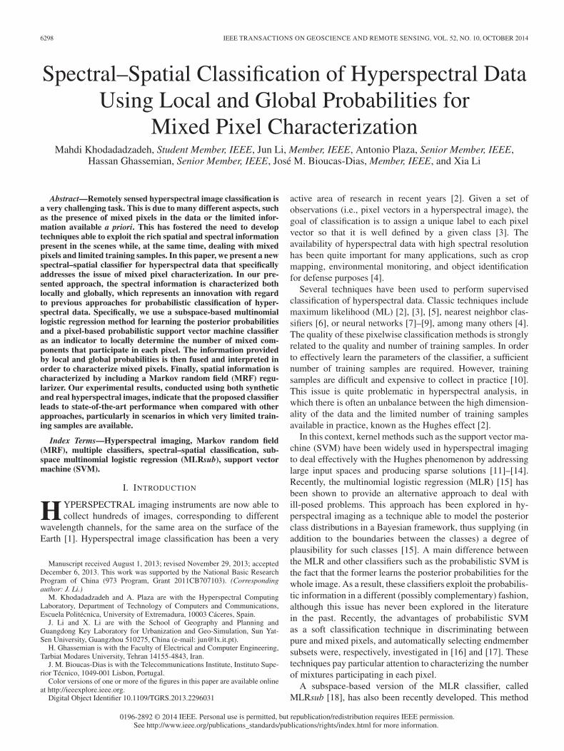
In this section, we describe the different components thathave been used in the development of the proposed method.First, we use probabilistic pixelwise classification methods tolearn the posterior probability distributions from the spectralinformation. Here, we use two strategies to characterize spectralinformation: probabilistic SVM and MLRsub. Then, we usecontextual information by means of an MRF regularizationscheme to refine the classification results. Fig. 1 shows therelationship between the methods considered in this study. Asit can be observed from Fig. 1, estimating class conditionalprobability distributions is an intrinsic issue for the subsequentMRF-based classification. In the following, we outline thedifferent strategies used to characterize spectral and spatialinformation, respectively, in the presented approach.

A. Characterization of Spectral Information

Let x ≡ {x1,x2, . . . ,xn} be the input hyperspectral image,where xi = [xi1,xi2, . . . ,xid]

T denotes a spectral vector asso-ciated with an image pixel i ∈ S, S = {1, 2, . . . , n} is the setof integers indexing the n pixels of x, and d is the number ofspectral bands. Let y ≡ (y1, . . . ,yn) denote an image of classlabels yi ≡ [yi1, yi2, . . . , yic . . . , yik]

T , where k is the num-ber of classes, yic = {0, 1}, for c = 1, . . . , k, and

∑c yic = 1.

Furthermore, let Dl ≡ {(x1,y1), . . . , (xl,yl)} be the labeledtraining set, with l being the number of samples in Dl. Withthe aforementioned definitions in mind, probabilistic pixelwise


Fig. 1. Relationship between the different components of the presented ap-proach for spectral–spatial classification of hyperspectral data.

classification intends to obtain, for a given pixel xi, the classlabel vector yi. This vector can be obtained by computing theposterior probability p(yic = 1|xi,Dl) as follows:

yic =

⎧⎨⎩

1, if p(yic = 1|xi,Dl) > p(yict = 1|xi,Dl)∀ ct �= c

0, otherwise.(1)

Various probabilistic classification techniques have beenused to process hyperspectral data [3]. In this paper, we usethe probabilistic SVM [39] and the MLRsub classifiers [18]for probability estimation. SVMs and MLRsub rely, respec-tively, on discriminant functions and posterior class distribu-tions which have shown good performance in hyperspectraldata classification, particularly in scenarios dominated by smalltraining samples. In the following, we describe these probabilis-tic classifiers in more details.

1) Probabilistic SVM Algorithm: The SVM classifier is typ-ically defined as follows [39]:

f(xj) =∑i

αiyiΦ(xi,xj) + b (2)

where xj ∈ x, xi ∈ Dl, b is the bias, and {αi}li=1 representsLagrange multipliers which are determined by the parameter C(that controls the amount of penalty during the SVM optimiza-tion). Here, Φ(xi,xj) is a function of the inputs, which can belinear or nonlinear. In SVM classification, kernel methods haveshown great advantage in comparison with linear methods [14].In this paper, we use a Gaussian radial basis function kernelK(xi,xj) = exp(−γ‖xi − xj‖2), whose width is controlledby parameter γ. Although the original SVM does not provideclass probability estimates, different techniques can be used toobtain class probability estimates based on combining all pair-wise comparisons [39]. In this paper, one of the probabilisticSVM methods [41] included in the popular LIBSVM library[42] is used.

2) MLRsub Algorithm: MLR-based techniques are able tomodel the posterior class distributions in a Bayesian frame-work. In these approaches, the densities p(yi|xi) are modeledwith the MLR, which corresponds to discriminative model ofthe discriminative–generative pair for p(xi|yi) Gaussian andp(yi) multinomial. The MLR model is formally given by [43]

p(yic = 1|xi,ω) =exp

(ω(c)h(c)(xi)

)∑k

c=1 exp(ω(c)h(xi)

) (3)

where h(c)(xi) ≡ [h(c)1 (xi), . . . ,h

(c)l (xi)]

T is a vector of lfixed functions of the input data, often termed as features;ω(c) is the set of logistic regressors for class c, and ω ≡[ω(1)T , . . . ,ω(c−1)T ]T . Recently, Li et al. [18] have proposedto combine MLR with a subspace projection method calledMLRsub to cope with two main issues: the presence of mixedpixels in hyperspectral data and the availability of limited train-ing samples. The idea of applying subspace projection methodsto improve classification relies on the basic assumption thatthe samples within each class can approximately lie in a lowerdimensional subspace. Thus, each class may be represented bya subspace spanned by a set of basis vectors, while the clas-sification criterion for a new input sample would be the distancefrom the class subspace [18]. In this formulation, the inputfunction is class dependent and is given by

h(c)(xi) =

[‖xi‖2,

∥∥∥xTi U

(c)∥∥∥2]T (4)

where U(c) = {u(c)1 , . . . ,u

(c)

r(k)} is a set of r(k)-dimensionalorthonormal basis vectors for the subspace associated with classc (r(c) � d).

B. Characterization of Spatial Information

In this section, we describe the mechanism used to includespatial–contextual information in the presented method. Forthis purpose, we use MRF, which is a widely used contextualmodel and a classical probabilistic method to model spatial cor-relation of pixel neighbors. This approach has been successfullyapplied in the context of remote sensing problems [35], [37],[41]. In the MRF framework, the MAP decision rule is typicallyformulated as the minimization of a suitable energy function[34]. Normally, the MRF-based approach can be implementedin two steps in hyperspectral image analysis. First, a probabilis-tic pixelwise classification method (such as those described inthe previous section) is applied to learn the posterior probabilitydistributions from the spectral information. Second, contextualinformation is included by means of an MRF regularization torefine the classification, as already outlined in Fig. 1.

According to the MAP-MRF framework, a pixel belongingto a class c is very likely to have neighboring pixels belongingto the same class. By using the Hammersley–Clifford theorem[45], we can write the MAP estimate of y as follows:

y = argminy

⎛⎝∑

i∈S− log p(yi|xi)− μ

∑i∼j

δ(yi − yj)

⎞⎠ (5)


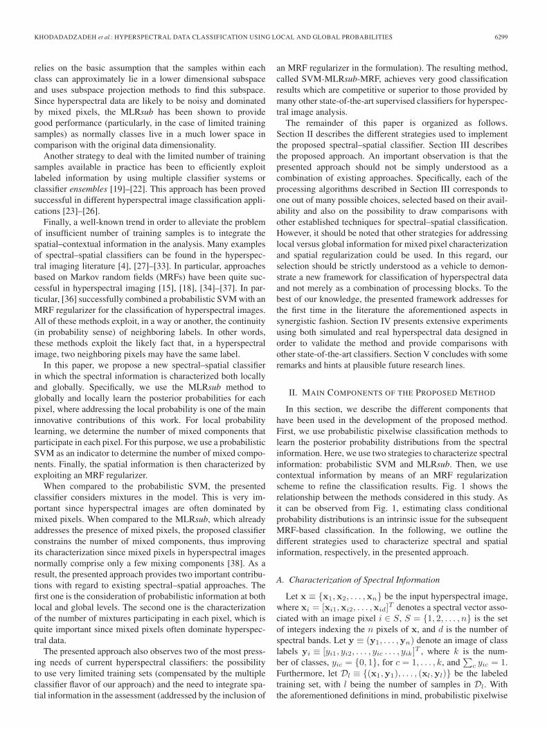
Fig. 2. Flowchart of the proposed SVM-MLRsub-MRF method.

where the term p(yi|xi) is the spectral energy function fromthe observed data, which needs to be estimated by probabilisticmethods. In this paper, we use the probabilistic SVM andMLRsub to learn the probabilities. Parameter μ is tunable andcontrols the degree of smoothness, and δ(y) is the unit impulsefunction, where δ(0) = 1 and δ(y) = 0 for y �= 0. Notice thatthe pairwise terms, δ(yi − yj), attach higher probability toequal neighboring labels than the other way around. Minimiza-tion of expression (5) is a combinatorial optimization probleminvolving unary and pairwise interaction terms. A good ap-proximation can be obtained by mapping the problem into thecomputation of a series of min-cuts on a suitable graphs [45].This aspect has been thoroughly explored in the context of hy-perspectral image classification in previous contributions [15].

III. PROPOSED APPROACH

In this section, we present the proposed spectral–spatialclassification approach called SVM-MLRsub-MRF. The fullmethodology is summarized by a detailed flowchart in Fig. 2.As shown in Fig. 2, the proposed approach mainly con-tains four steps: 1) generation of the class combination map;2) calculation of the local and global probabilities; 3) decisionfusion; and 4) MRF regularization. In the following, we presentthe details of each individual steps.

A. Generation of the Class Combination Map

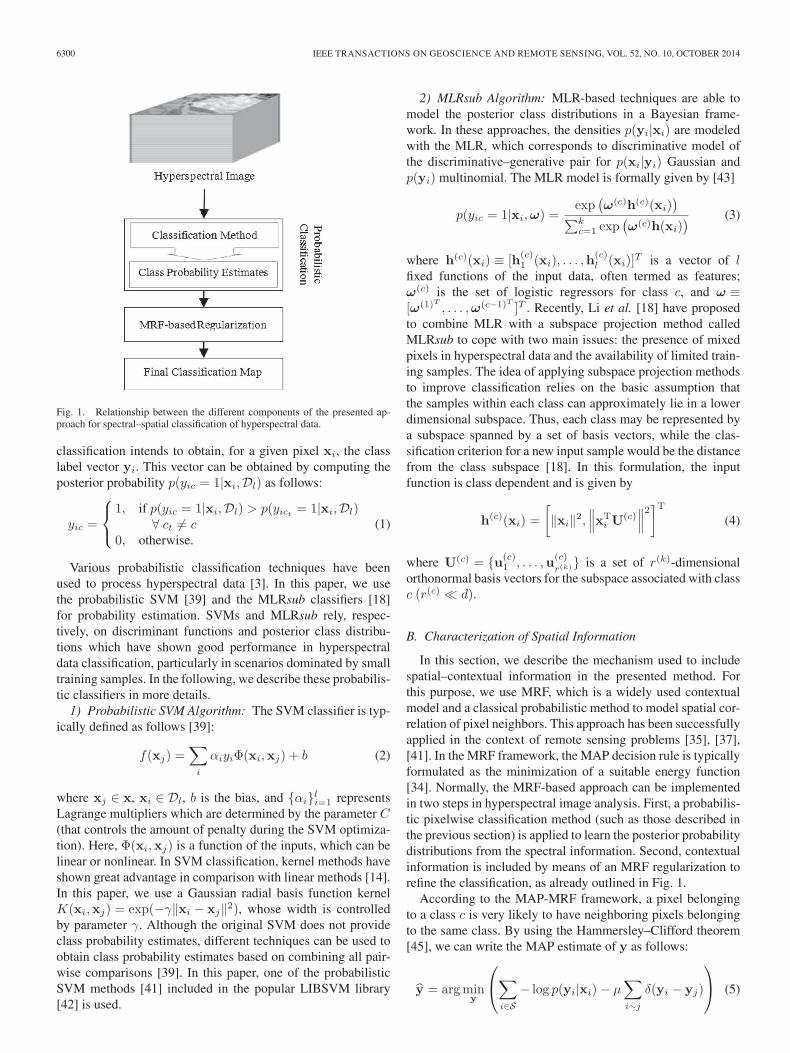
The class combination map is generated from the proba-bilistic SVM classification results. Notice that the probabilisticSVM is only used as an indicator to determine the number ofmixtures appearing in each pixel and does not contribute to theprobability learning. For this purpose, a subset of the M mostreliable class labels (mixed components) is chosen for eachpixel as the possible class combinations for that pixel, and M ≤k. In case M = k, the local learning is equivalent to the globallearning. It is also important to emphasize that, although in thiswork we use the probabilistic SVM for pixelwise classificationdue to its proved effectiveness in hyperspectral classification[14], other probabilistic classifiers could also be used as far asthey are well suited to hyperspectral analysis. Furthermore, asa classifier, the probabilistic SVM has different characteristics

Fig. 3. Example of the generation of a class combination map using thresholdM = 2.

in comparison with MLRsub, thus allowing for the possibilityto use both classifiers in combined fashion in order to removeirrelevant class labels and to improve the efficiency of the class-dependent subspace projection step in the MLRsub method,which will be described in the following section.

For illustrative purposes, Fig. 3 shows an example of howto generate a class combination map using the aforementionedstrategy for a three-class problem, where the classes are denotedas {A,B,C} and the number of mixed components is set toM = 2. Using the probabilistic SVM, for each pixel, we obtaina vector of three probabilities with respect to classes A, B, andC. As shown in Fig. 3, for the pixel at the top-right corner of theimage, we assume that the probabilities are 0.3, 0.1, and 0.6 (forclasses A, B, and C, respectively). Under these assumptions,the pixel would be assigned to the subset {A,C} (from allpossible combinations of the three classes). Notice that, in thisexample, there is no pixel assigned to the class combination{B,C}. Finally, it should be noted that the number of classcombinations is given by C(k,M), where, in this example, it isC(3, 2) = 3.

B. Calculation of the Local and Global Probabilities

In this section, we describe the procedure used to calculatethe local and global probabilities. Here, we use the MLRsubalgorithm to learn the posterior probability distributions locallyfor the M classes selected in the previous step and globally forall classes. Let pg and pl denote the global and local posteriorprobabilities, respectively. For example, if we take the pixel


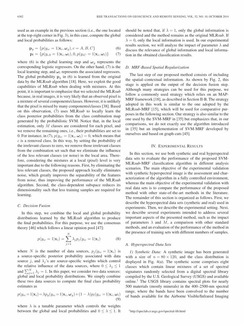
used as an example in the previous section (i.e., the one locatedat the top-right corner in Fig. 3), in this case, compute the globaland local probabilities as follows:

pg = {p(yic = 1|xi,ωg), c = A,B,C} (6)

pl = {p(yiA = 1|xi,ωl), 0, p(yiC = 1|xi,ωl)} (7)

where (6) is the global learning step and ωg represents thecorresponding logistic regressors. On the other hand, (7) is thelocal learning step, and ωl represents the associated regressors.The global probability pg in (6) is learned from the originaldata by the MLRsub algorithm [18]. Here, we exploit the goodcapabilities of MLRsub when dealing with mixtures. At thispoint, it is important to emphasize that we selected the MLRsubbecause, in real images, it is very likely that an observed pixel isa mixture of several components/classes. However, it is unlikelythat the pixel is mixed by many components/classes [38]. Basedon this observation, (7) uses MLRsub to locally learn theclass posterior probabilities from the class combination mapgenerated by the probabilistic SVM. Notice that, in the localestimation, only M classes are considered for each pixel, andwe remove the remaining ones, i.e., their probabilities are set to0. For instance, in (7), p(yic = 1|xi,ωl) = 0, which means thatc is a removed class. In this way, by setting the probability ofthe irrelevant classes to zero, we remove those irrelevant classesfrom the combination set such that we eliminate the influenceof the less relevant classes (or noise) in the local area. There-fore, considering the mixtures at a local (pixel) level is veryimportant due to the following reasons. First, by eliminating theless relevant classes, the proposed approach locally eliminatesnoise, which greatly improves the separability of the featuresfrom noise, thus improving the performance of the MLRsubalgorithm. Second, the class-dependent subspace reduces itsdimensionality such that less training samples are required forlearning.

C. Decision Fusion

In this step, we combine the local and global probabilitydistributions learned by the MLRsub algorithm to producethe final probabilities. For this purpose, we use the consensustheory [46] which follows a linear opinion pool [47]:

p(yic = 1|xi) =

N∑j=1

λjpj(yic = 1|xi) (8)

where N is the number of data sources, pj(yic = 1|xi) isa source-specific posterior probability associated with datasource j, and λj’s are source-specific weights which controlthe relative influence of the data sources, where 0 ≤ λj ≤ 1

and∑N

j=1 λj = 1. In this paper, we consider two data sources:global and local probability distributions. We simply combinethese two data sources to compute the final class probabilityestimates as

p(yic=1|xi)=λpg(yic=1|xi,ωg)+(1− λ)pl(yic =1|xi,ωl)(9)

where λ is a tunable parameter which controls the weightsbetween the global and local probabilities and 0 ≤ λ ≤ 1. It

should be noted that, if λ = 1, only the global information isconsidered and the method remains as the original MLRsub. Ifλ = 0, only the local information is used. In our experimentalresults section, we will analyze the impact of parameter λ anddiscuss the relevance of global information and local informa-tion in the obtained classification results.

D. MRF-Based Spatial Regularization

The last step of our proposed method consists of includingthe spatial–contextual information. As shown by Fig. 2, thisstage is applied on the output of the decision fusion step.Although many strategies can be used for this purpose, wefollow a commonly used strategy which relies on an MAP-MRF framework [18], as described in Section II-B. The strategyadopted in this work is similar to the one adopted by theMLRsub-MRF [15], which will be used for comparative pur-poses in the following section. Our strategy is also similar to theone used by the SVM-MRF in [35] but emphasizes that, in ourcomparisons, we do not exactly use the algorithm introducedin [35] but an implementation of SVM-MRF developed byourselves and based on graph-cuts [45].

IV. EXPERIMENTAL RESULTS

In this section, we use both synthetic and real hyperspectraldata sets to evaluate the performance of the proposed SVM-MLRsub-MRF classification algorithm in different analysisscenarios. The main objective of the experimental validationwith synthetic hyperspectral image is the assessment and char-acterization of the algorithm in a fully controlled environment,whereas the main objective of the experimental validation withreal data sets is to compare the performance of the proposedmethod with other state-of-the-art methods in the literature.The remainder of this section is organized as follows. First, wedescribe the hyperspectral data sets (synthetic and real) used inexperiments. Then, we describe the experimental setting. Next,we describe several experiments intended to address severalimportant aspects of the presented method, such as the impactof parameters λ and M , a comparison with other standardmethods, and an evaluation of the performance of the method inthe presence of training sets with different numbers of samples.

A. Hyperspectral Data Sets

1) Synthetic Data: A synthetic image has been generatedwith a size of n = 80× 120, and the class distribution isdisplayed in Fig. 4(a). The synthetic scene comprises eightclasses which contain linear mixtures of a set of spectralsignatures randomly selected from a digital spectral librarycompiled by the U.S. Geological Survey (USGS) and availableonline.1 The USGS library contains spectral plots for nearly500 materials (mostly minerals) in the 400–2500-nm spectralrange, where the bands have been convolved to the numberof bands available for the Airborne Visible/Infrared Imaging

1http://speclab.cr.usgs.gov/spectral-lib.html


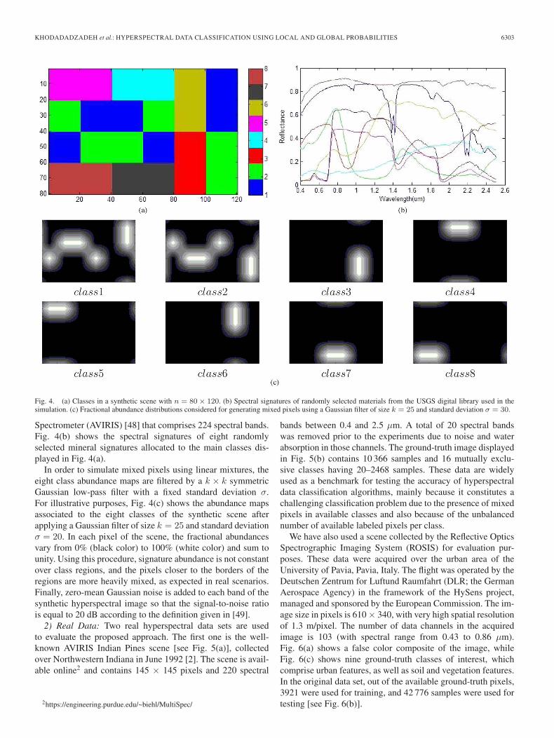
Fig. 4. (a) Classes in a synthetic scene with n = 80× 120. (b) Spectral signatures of randomly selected materials from the USGS digital library used in thesimulation. (c) Fractional abundance distributions considered for generating mixed pixels using a Gaussian filter of size k = 25 and standard deviation σ = 30.

Spectrometer (AVIRIS) [48] that comprises 224 spectral bands.Fig. 4(b) shows the spectral signatures of eight randomlyselected mineral signatures allocated to the main classes dis-played in Fig. 4(a).

In order to simulate mixed pixels using linear mixtures, theeight class abundance maps are filtered by a k × k symmetricGaussian low-pass filter with a fixed standard deviation σ.For illustrative purposes, Fig. 4(c) shows the abundance mapsassociated to the eight classes of the synthetic scene afterapplying a Gaussian filter of size k = 25 and standard deviationσ = 20. In each pixel of the scene, the fractional abundancesvary from 0% (black color) to 100% (white color) and sum tounity. Using this procedure, signature abundance is not constantover class regions, and the pixels closer to the borders of theregions are more heavily mixed, as expected in real scenarios.Finally, zero-mean Gaussian noise is added to each band of thesynthetic hyperspectral image so that the signal-to-noise ratiois equal to 20 dB according to the definition given in [49].

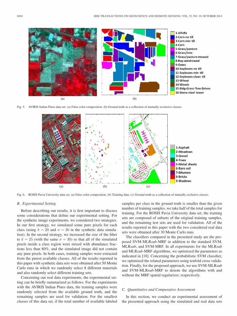
2) Real Data: Two real hyperspectral data sets are usedto evaluate the proposed approach. The first one is the well-known AVIRIS Indian Pines scene [see Fig. 5(a)], collectedover Northwestern Indiana in June 1992 [2]. The scene is avail-able online2 and contains 145 × 145 pixels and 220 spectral

2https://engineering.purdue.edu/~biehl/MultiSpec/

bands between 0.4 and 2.5 μm. A total of 20 spectral bandswas removed prior to the experiments due to noise and waterabsorption in those channels. The ground-truth image displayedin Fig. 5(b) contains 10 366 samples and 16 mutually exclu-sive classes having 20–2468 samples. These data are widelyused as a benchmark for testing the accuracy of hyperspectraldata classification algorithms, mainly because it constitutes achallenging classification problem due to the presence of mixedpixels in available classes and also because of the unbalancednumber of available labeled pixels per class.

We have also used a scene collected by the Reflective OpticsSpectrographic Imaging System (ROSIS) for evaluation pur-poses. These data were acquired over the urban area of theUniversity of Pavia, Pavia, Italy. The flight was operated by theDeutschen Zentrum for Luftund Raumfahrt (DLR; the GermanAerospace Agency) in the framework of the HySens project,managed and sponsored by the European Commission. The im-age size in pixels is 610 × 340, with very high spatial resolutionof 1.3 m/pixel. The number of data channels in the acquiredimage is 103 (with spectral range from 0.43 to 0.86 μm).Fig. 6(a) shows a false color composite of the image, whileFig. 6(c) shows nine ground-truth classes of interest, whichcomprise urban features, as well as soil and vegetation features.In the original data set, out of the available ground-truth pixels,3921 were used for training, and 42 776 samples were used fortesting [see Fig. 6(b)].


Fig. 5. AVIRIS Indian Pines data set. (a) False color composition. (b) Ground truth as a collection of mutually exclusive classes.

Fig. 6. ROSIS Pavia University data set. (a) False color composition. (b) Training data. (c) Ground truth as a collection of mutually exclusive classes.

B. Experimental Setting

Before describing our results, it is first important to discusssome considerations that define our experimental setting. Forthe synthetic image experiments, we considered two strategies.In our first strategy, we simulated some pure pixels for eachclass (using k = 20 and σ = 30 in the synthetic data simula-tion). In the second strategy, we increased the size of the filterto k = 25 (with the same σ = 30) so that all of the simulatedpixels inside a class region were mixed with abundance frac-tions less than 80%, and the simulated image did not containany pure pixels. In both cases, training samples were extractedfrom the purest available classes. All of the results reported inthis paper with synthetic data sets were obtained after 50 MonteCarlo runs in which we randomly select 8 different materialsand also randomly select different training sets.

Concerning our real data experiments, the experimental set-ting can be briefly summarized as follows. For the experimentswith the AVIRIS Indian Pines data, the training samples wererandomly selected from the available ground truth, and theremaining samples are used for validation. For the smallestclasses of this data set, if the total number of available labeled

samples per class in the ground truth is smaller than the givennumber of training samples, we take half of the total samples fortraining. For the ROSIS Pavia University data set, the trainingsets are composed of subsets of the original training samples,and the remaining test sets are used for validation. All of theresults reported in this paper with the two considered real datasets were obtained after 30 Monte Carlo runs.

The classifiers compared in the presented study are the pro-posed SVM-MLRsub-MRF in addition to the standard SVM,MLRsub, and SVM-MRF. In all experiments for the MLRsuband MLRsub-MRF algorithms, we optimized the parameters asindicated in [18]. Concerning the probabilistic SVM classifier,we optimized the related parameters using tenfold cross valida-tion. Finally, for the proposed approach, we use SVM-MLRsuband SVM-MLRsub-MRF to denote the algorithms with andwithout the MRF spatial regularizer, respectively.

C. Quantitative and Comparative Assessment

In this section, we conduct an experimental assessment ofthe presented approach using the simulated and real data sets


TABLE IOVERALL (OA) AND AVERAGE (AA) CLASSIFICATION ACCURACIES (IN PERCENT; AS A FUNCTION OF PARAMETER λ) OBTAINED BY THE

SVM-MLRsub-MRF METHOD FOR THE SYNTHETIC AND REAL DATA SETS CONSIDERED IN THE EXPERIMENTS.THE BEST RESULTS ARE OUTLINED IN BOLD TYPEFACE

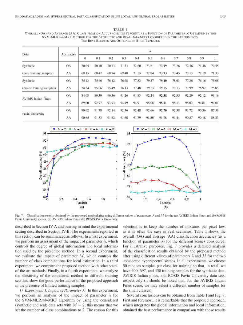
Fig. 7. Classification results obtained by the proposed method after using different values of parameters λ and M for the (a) AVIRIS Indian Pines and (b) ROSISPavia University scenes. (a) AVIRIS Indian Pines. (b) ROSIS Pavia University.

described in Section IV-A and bearing in mind the experimentalsetting described in Section IV-B. The experiments reported inthis section can be summarized as follows. In a first experiment,we perform an assessment of the impact of parameter λ, whichcontrols the degree of global information and local informa-tion used by the presented method. In a second experiment,we evaluate the impact of parameter M , which controls thenumber of class combinations for local estimation. In a thirdexperiment, we compare the proposed method with other state-of-the-art methods. Finally, in a fourth experiment, we analyzethe sensitivity of the considered method to different trainingsets and show the good performance of the proposed approachin the presence of limited training samples.

1) Experiment 1. Impact of Parameter λ: In this experiment,we perform an analysis of the impact of parameter λ forthe SVM-MLRsub-MRF algorithm by using the considered(synthetic and real) data sets with M = 2; this means that weset the number of class combinations to 2. The reason for this

selection is to keep the number of mixtures per pixel low,as it is often the case in real scenarios. Table I shows theoverall (OA) and average (AA) classification accuracies (as afunction of parameter λ) for the different scenes considered.For illustrative purposes, Fig. 7 provides a detailed analysisof the classification results obtained by the proposed methodafter using different values of parameters λ and M for the twoconsidered hyperspectral scenes. In all experiments, we choose50 random samples per class for training so that, in total, wehave 400, 697, and 450 training samples for the synthetic data,AVIRIS Indian pines, and ROSIS Pavia University data sets,respectively (it should be noted that, for the AVIRIS IndianPines scene, we may select a different number of samples forthe small classes).

Several conclusions can be obtained from Table I and Fig. 7.First and foremost, it is remarkable that the proposed approach,which integrates the global information and local information,obtained the best performance in comparison with those results


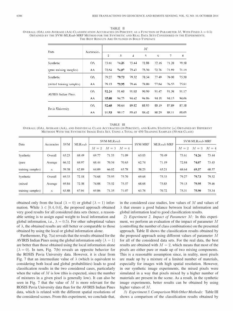
TABLE IIOVERALL (OA) AND AVERAGE (AA) CLASSIFICATION ACCURACIES (IN PERCENT; AS A FUNCTION OF PARAMETER M , WITH FIXED λ = 0.5)

OBTAINED BY THE SVM-MLRsub-MRF METHOD FOR THE SYNTHETIC AND REAL DATA SETS CONSIDERED IN THE EXPERIMENTS.THE BEST RESULTS ARE OUTLINED IN BOLD TYPEFACE

TABLE IIIOVERALL (OA), AVERAGE (AA), AND INDIVIDUAL CLASS ACCURACIES (IN PERCENT), AND KAPPA STATISTIC (κ) OBTAINED BY DIFFERENT

METHODS WITH THE SYNTHETIC IMAGE DATA SET, USING A TOTAL OF 450 TRAINING SAMPLES (50 PER CLASS)

obtained only from the local (λ = 0) or global (λ = 1) infor-mation. While λ ∈ [0.4, 0.6], the proposed approach obtainedvery good results for all considered data sets (hence, a reason-able setting is to assign equal weight to local information andglobal information, i.e., λ = 0.5). For other suboptimal valuesof λ, the obtained results are still better or comparable to thoseobtained by using the local or global information alone.

Furthermore, Fig. 7(a) reveals that the results obtained for theAVIRIS Indian Pines using the global information only (λ = 1)are better than those obtained using the local information alone(λ = 0). In turn, Fig. 7(b) reveals an opposite behavior forthe ROSIS Pavia University data. However, it is clear fromFig. 7 that an intermediate value of λ (which is equivalent toconsidering both local and global probabilities) leads to goodclassification results in the two considered cases, particularlywhen the value of M is low (this is expected, since the numberof mixtures in a given pixel is generally low). It can also beseen in Fig. 7 that the value of M is more relevant for theROSIS Pavia University data than for the AVIRIS Indian Pinesdata, which is related with the different spatial resolutions ofthe considered scenes. From this experiment, we conclude that,

in the considered case studies, low values of M and values ofλ that ensure a good balance between local information andglobal information lead to good classification results.

2) Experiment 2. Impact of Parameter M : In this experi-ment, we perform an evaluation of the impact of parameter M(controlling the number of class combinations) on the presentedapproach. Table II shows the classification results obtained bythe proposed approach using different values of parameter Mfor all of the considered data sets. For the real data, the bestresults are obtained with M = 2, which means that most of thepixels are either pure or made up of two mixing components.This is a reasonable assumption since, in reality, most pixelsare made up by a mixture of a limited number of materials,especially for images with high spatial resolution. However,in our synthetic image experiments, the mixed pixels weresimulated in a way that pixels mixed by a higher number ofmaterials are present in the scene. As a result, in the syntheticimage experiments, better results can be obtained by usinghigher values of M .

3) Experiment 3. Comparison With Other Methods: Table IIIshows a comparison of the classification results obtained by


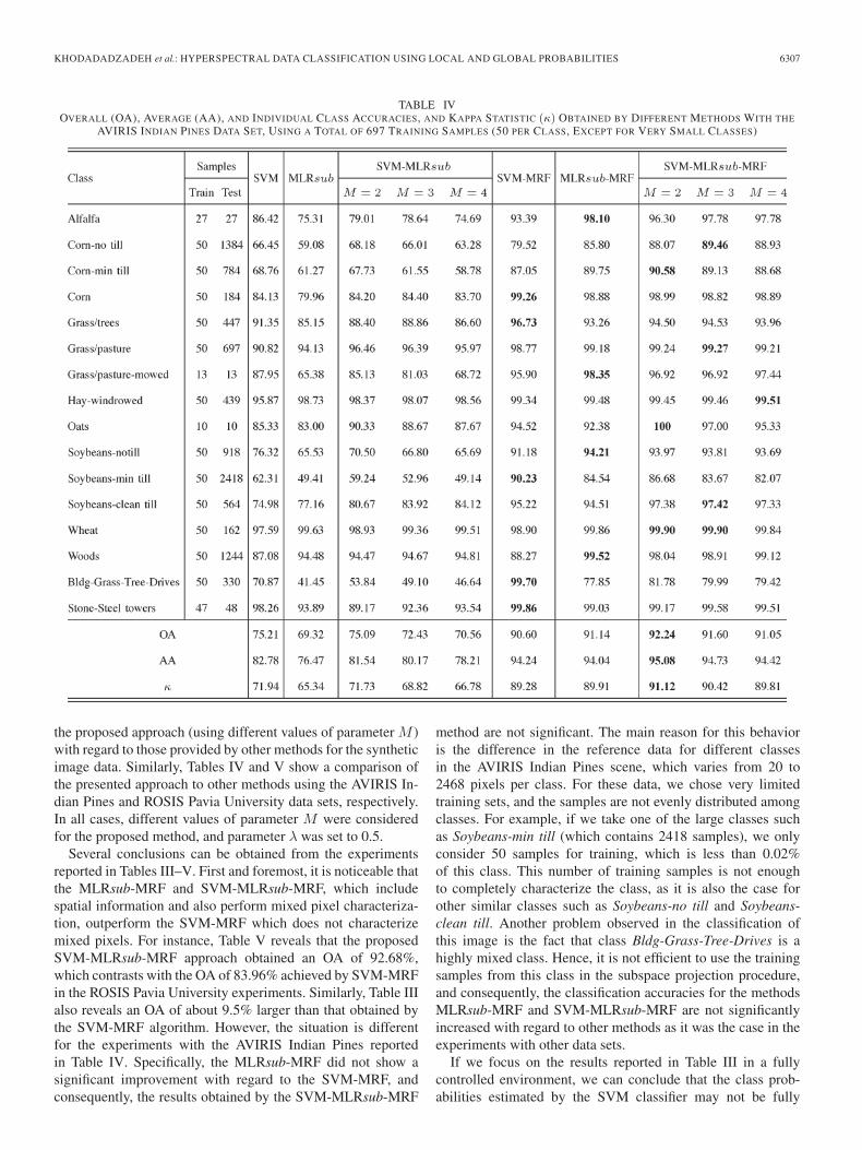
TABLE IVOVERALL (OA), AVERAGE (AA), AND INDIVIDUAL CLASS ACCURACIES, AND KAPPA STATISTIC (κ) OBTAINED BY DIFFERENT METHODS WITH THE

AVIRIS INDIAN PINES DATA SET, USING A TOTAL OF 697 TRAINING SAMPLES (50 PER CLASS, EXCEPT FOR VERY SMALL CLASSES)

the proposed approach (using different values of parameter M )with regard to those provided by other methods for the syntheticimage data. Similarly, Tables IV and V show a comparison ofthe presented approach to other methods using the AVIRIS In-dian Pines and ROSIS Pavia University data sets, respectively.In all cases, different values of parameter M were consideredfor the proposed method, and parameter λ was set to 0.5.

Several conclusions can be obtained from the experimentsreported in Tables III–V. First and foremost, it is noticeable thatthe MLRsub-MRF and SVM-MLRsub-MRF, which includespatial information and also perform mixed pixel characteriza-tion, outperform the SVM-MRF which does not characterizemixed pixels. For instance, Table V reveals that the proposedSVM-MLRsub-MRF approach obtained an OA of 92.68%,which contrasts with the OA of 83.96% achieved by SVM-MRFin the ROSIS Pavia University experiments. Similarly, Table IIIalso reveals an OA of about 9.5% larger than that obtained bythe SVM-MRF algorithm. However, the situation is differentfor the experiments with the AVIRIS Indian Pines reportedin Table IV. Specifically, the MLRsub-MRF did not show asignificant improvement with regard to the SVM-MRF, andconsequently, the results obtained by the SVM-MLRsub-MRF

method are not significant. The main reason for this behavioris the difference in the reference data for different classesin the AVIRIS Indian Pines scene, which varies from 20 to2468 pixels per class. For these data, we chose very limitedtraining sets, and the samples are not evenly distributed amongclasses. For example, if we take one of the large classes suchas Soybeans-min till (which contains 2418 samples), we onlyconsider 50 samples for training, which is less than 0.02%of this class. This number of training samples is not enoughto completely characterize the class, as it is also the case forother similar classes such as Soybeans-no till and Soybeans-clean till. Another problem observed in the classification ofthis image is the fact that class Bldg-Grass-Tree-Drives is ahighly mixed class. Hence, it is not efficient to use the trainingsamples from this class in the subspace projection procedure,and consequently, the classification accuracies for the methodsMLRsub-MRF and SVM-MLRsub-MRF are not significantlyincreased with regard to other methods as it was the case in theexperiments with other data sets.

If we focus on the results reported in Table III in a fullycontrolled environment, we can conclude that the class prob-abilities estimated by the SVM classifier may not be fully


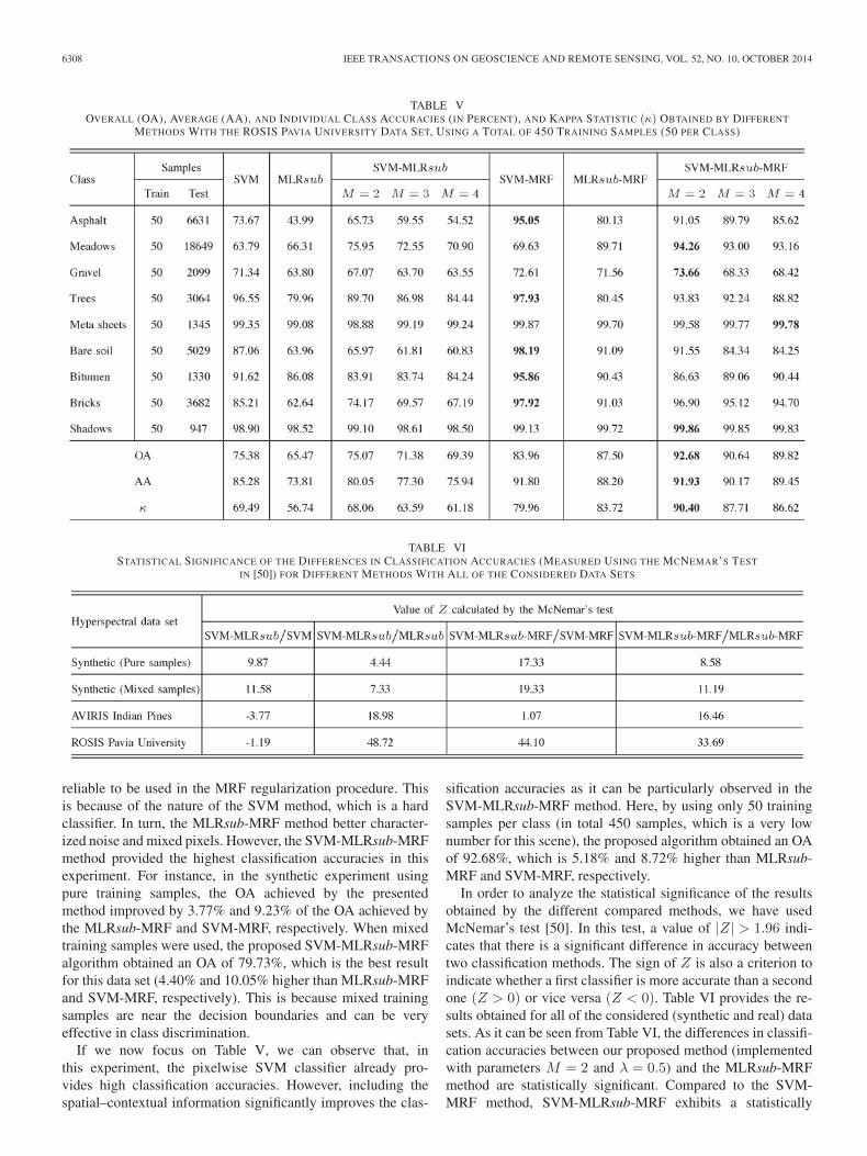
TABLE VOVERALL (OA), AVERAGE (AA), AND INDIVIDUAL CLASS ACCURACIES (IN PERCENT), AND KAPPA STATISTIC (κ) OBTAINED BY DIFFERENT

METHODS WITH THE ROSIS PAVIA UNIVERSITY DATA SET, USING A TOTAL OF 450 TRAINING SAMPLES (50 PER CLASS)

TABLE VISTATISTICAL SIGNIFICANCE OF THE DIFFERENCES IN CLASSIFICATION ACCURACIES (MEASURED USING THE MCNEMAR’S TEST

IN [50]) FOR DIFFERENT METHODS WITH ALL OF THE CONSIDERED DATA SETS

reliable to be used in the MRF regularization procedure. Thisis because of the nature of the SVM method, which is a hardclassifier. In turn, the MLRsub-MRF method better character-ized noise and mixed pixels. However, the SVM-MLRsub-MRFmethod provided the highest classification accuracies in thisexperiment. For instance, in the synthetic experiment usingpure training samples, the OA achieved by the presentedmethod improved by 3.77% and 9.23% of the OA achieved bythe MLRsub-MRF and SVM-MRF, respectively. When mixedtraining samples were used, the proposed SVM-MLRsub-MRFalgorithm obtained an OA of 79.73%, which is the best resultfor this data set (4.40% and 10.05% higher than MLRsub-MRFand SVM-MRF, respectively). This is because mixed trainingsamples are near the decision boundaries and can be veryeffective in class discrimination.

If we now focus on Table V, we can observe that, inthis experiment, the pixelwise SVM classifier already pro-vides high classification accuracies. However, including thespatial–contextual information significantly improves the clas-

sification accuracies as it can be particularly observed in theSVM-MLRsub-MRF method. Here, by using only 50 trainingsamples per class (in total 450 samples, which is a very lownumber for this scene), the proposed algorithm obtained an OAof 92.68%, which is 5.18% and 8.72% higher than MLRsub-MRF and SVM-MRF, respectively.

In order to analyze the statistical significance of the resultsobtained by the different compared methods, we have usedMcNemar’s test [50]. In this test, a value of |Z| > 1.96 indi-cates that there is a significant difference in accuracy betweentwo classification methods. The sign of Z is also a criterion toindicate whether a first classifier is more accurate than a secondone (Z > 0) or vice versa (Z < 0). Table VI provides the re-sults obtained for all of the considered (synthetic and real) datasets. As it can be seen from Table VI, the differences in classifi-cation accuracies between our proposed method (implementedwith parameters M = 2 and λ = 0.5) and the MLRsub-MRFmethod are statistically significant. Compared to the SVM-MRF method, SVM-MLRsub-MRF exhibits a statistically


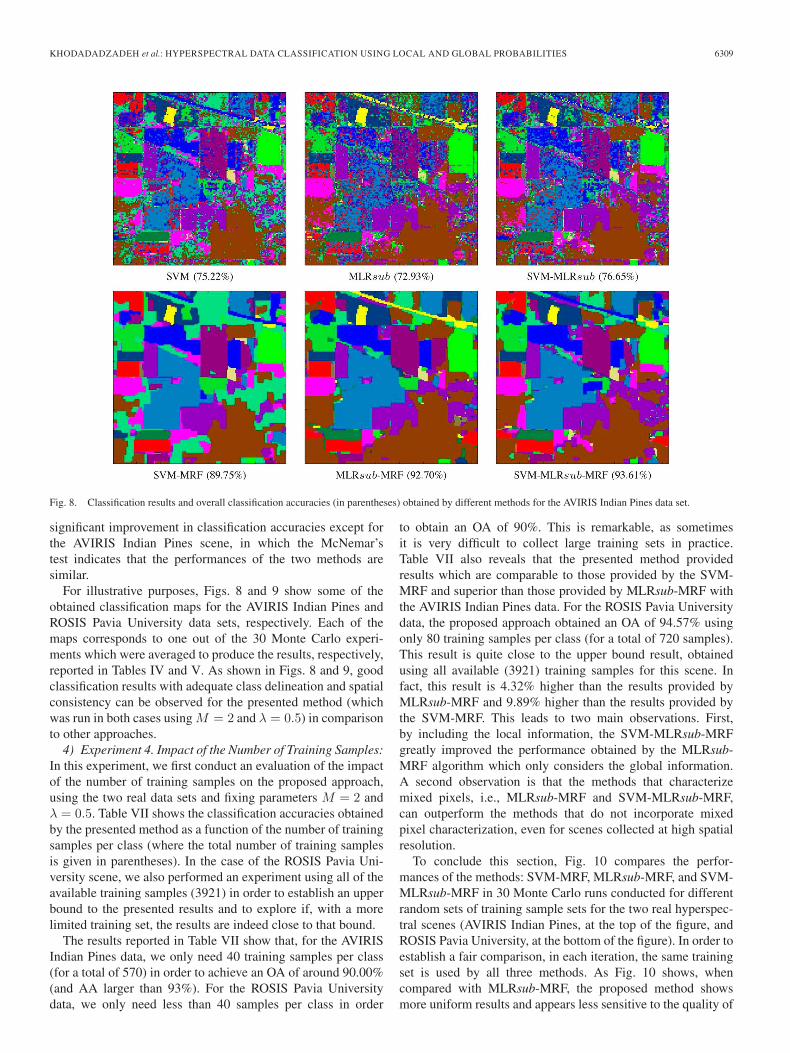
Fig. 8. Classification results and overall classification accuracies (in parentheses) obtained by different methods for the AVIRIS Indian Pines data set.

significant improvement in classification accuracies except forthe AVIRIS Indian Pines scene, in which the McNemar’stest indicates that the performances of the two methods aresimilar.

For illustrative purposes, Figs. 8 and 9 show some of theobtained classification maps for the AVIRIS Indian Pines andROSIS Pavia University data sets, respectively. Each of themaps corresponds to one out of the 30 Monte Carlo experi-ments which were averaged to produce the results, respectively,reported in Tables IV and V. As shown in Figs. 8 and 9, goodclassification results with adequate class delineation and spatialconsistency can be observed for the presented method (whichwas run in both cases using M = 2 and λ = 0.5) in comparisonto other approaches.

4) Experiment 4. Impact of the Number of Training Samples:In this experiment, we first conduct an evaluation of the impactof the number of training samples on the proposed approach,using the two real data sets and fixing parameters M = 2 andλ = 0.5. Table VII shows the classification accuracies obtainedby the presented method as a function of the number of trainingsamples per class (where the total number of training samplesis given in parentheses). In the case of the ROSIS Pavia Uni-versity scene, we also performed an experiment using all of theavailable training samples (3921) in order to establish an upperbound to the presented results and to explore if, with a morelimited training set, the results are indeed close to that bound.

The results reported in Table VII show that, for the AVIRISIndian Pines data, we only need 40 training samples per class(for a total of 570) in order to achieve an OA of around 90.00%(and AA larger than 93%). For the ROSIS Pavia Universitydata, we only need less than 40 samples per class in order

to obtain an OA of 90%. This is remarkable, as sometimesit is very difficult to collect large training sets in practice.Table VII also reveals that the presented method providedresults which are comparable to those provided by the SVM-MRF and superior than those provided by MLRsub-MRF withthe AVIRIS Indian Pines data. For the ROSIS Pavia Universitydata, the proposed approach obtained an OA of 94.57% usingonly 80 training samples per class (for a total of 720 samples).This result is quite close to the upper bound result, obtainedusing all available (3921) training samples for this scene. Infact, this result is 4.32% higher than the results provided byMLRsub-MRF and 9.89% higher than the results provided bythe SVM-MRF. This leads to two main observations. First,by including the local information, the SVM-MLRsub-MRFgreatly improved the performance obtained by the MLRsub-MRF algorithm which only considers the global information.A second observation is that the methods that characterizemixed pixels, i.e., MLRsub-MRF and SVM-MLRsub-MRF,can outperform the methods that do not incorporate mixedpixel characterization, even for scenes collected at high spatialresolution.

To conclude this section, Fig. 10 compares the perfor-mances of the methods: SVM-MRF, MLRsub-MRF, and SVM-MLRsub-MRF in 30 Monte Carlo runs conducted for differentrandom sets of training sample sets for the two real hyperspec-tral scenes (AVIRIS Indian Pines, at the top of the figure, andROSIS Pavia University, at the bottom of the figure). In order toestablish a fair comparison, in each iteration, the same trainingset is used by all three methods. As Fig. 10 shows, whencompared with MLRsub-MRF, the proposed method showsmore uniform results and appears less sensitive to the quality of


Fig. 9. Classification results and overall classification accuracies (in parentheses) obtained by different methods for the ROSIS Pavia University data set.

training samples. When compared with SVM-MRF, the pro-posed method shows slightly superior results for the AVIRISIndian Pines scene and consistently better performance for thePavia University scene. Again, we reiterate that the SVM-MLRsub method takes the advantages of both SVM andMLRsub and can compensate the situation in which one ofthe methods does not provide good performance by takingadvantage of the other method. This is also the reason whythe proposed SVM-MLRsub-MRF method can provide goodperformance in those cases in which none of the methods SVM-MRF and MLRsub-MRF exhibits good classification accura-cies. This is the case, for instance, in iterations 6, 13, and 25 forthe ROSIS Pavia University experiments reported in Fig. 10.

V. CONCLUSION AND FUTURE RESEARCH LINES

In this paper, we have introduced a novel spectral–spatialclassifier for hyperspectral image data. The proposed methodis based on the consideration of both global posterior probabil-ity distributions and local probabilities which result from the

whole image and a set of previously derived class combina-tion maps, respectively. The proposed approach, which intendsto characterize mixed pixels in the scene and assumes thatthese pixels are normally mixed by only a few components,provides some distinguishing features with regard to otherexisting approaches. At the local learning level, the presentedmethod removes the impact of irrelevant classes by means of apreprocessing stage (implemented using the probabilistic SVM)intended to produce a subset of M most probable classes foreach pixel.

This stage locally eliminates noise and enhances the impactof the most relevant classes. These aspects, together with thejoint characterization of mixed pixels and spatial–contextualinformation, make our method unique and representative of aframework that, for the first time in the literature, integrateslocal and global probabilities in the analysis of hyperspectraldata in order to constrain the number of mixing componentsused in the characterization of mixed pixels. This is consistentwith the observation that, despite the presence of mixed pixelsin real hyperspectral scenes, it is reasonable to assume that the


TABLE VIIOVERALL (OA) AND AVERAGE (AA) ACCURACY (IN PERCENT) AS A FUNCTION OF THE NUMBER OF TRAINING SAMPLES PER CLASS FOR THE

SVM-MLRsub-MRF METHOD, WHERE THE TOTAL NUMBER OF TRAINING SAMPLES IS GIVEN IN PARENTHESES

Fig. 10. Comparison of the performances of the methods: SVM-MRF, MLRsub-MRF, and SVM-MLRsub-MRF in 30 Monte Carlo runs conducted for differentrandom sets of training sample sets for the two real hyperspectral scenes: (top) AVIRIS Indian Pines and (bottom) ROSIS Pavia University. In each run, the sametraining set is used by all three methods.

mixing components in a given pixel are limited. Our experi-mental results, conducted using both synthetic and real hyper-spectral scenes widely used in the hyperspectral classificationcommunity, indicate that the proposed approach leads to state-of-the-art performance when compared with other approaches,

particularly in scenarios in which very limited training samplesare available.

As future research, we are currently developing a version ofthe presented algorithm in which parameter M is adaptivelyestimated for each pixel rather than set in advance as in the


version of the algorithm reported in this paper. Interestingly,we have empirically observed that the adaptive selection pro-duces similar results to those obtained in this work with fixedparameter settings such as M = 2 or M = 3, which result inmuch lower computational cost than an adaptive estimation ofthe parameter on a per-pixel basis. As a result, we will continueexploring the possibility to select this parameter adaptivelyin order to improve the obtained classification results withoutincreasing computational complexity, which currently stays onthe same order of magnitude as the other methods used in thecomparisons reported in this work. In future developments, wewill further explore the relationship between the parametersof our method and the spatial resolution, level of noise, andcomplexity of the analyzed scenes. We are also planning onexploring the applications of the presented method for theanalysis of multitemporal data sets.

ACKNOWLEDGMENT

The authors would like to thank Prof. D. Landgrebe for mak-ing the AVIRIS Indian Pines hyperspectral data set availableto the community, Prof. P. Gamba for providing the ROSISdata over University of Pavia, Pavia, Italy, along with thetraining and test sets, and the Associate Editor who handledthis paper and the three anonymous reviewers for providingtruly outstanding comments and suggestions that significantlyhelped in improving the technical quality and presentation ofthis paper.

REFERENCES

[1] C.-I. Chang, Hyperspectral Data Exploitation: Theory and Applications.New York, NY, USA: Wiley, 2007.

[2] D. A. Landgrebe, Signal Theory Methods in Multispectral Remote Sens-ing. Hoboken, NJ, USA: Wiley, 2003.

[3] J. A. Richards and X. Jia, Remote Sensing Digital Image Analysis., 4th ed.Berlin, Germany: Springer-Verlag, 2006.

[4] A. Plaza, J. A. Benediktsson, J. Boardman, J. Brazile, L. Bruzzone,G. Camps-Valls, J. Chanussot, M. Fauvel, P. Gamba, J. A. Gualtieri,M. Marconcini, J. C. Tilton, and G. Trianni, “Recent advances in tech-niques for hyperspectral image processing,” Remote Sens. Environ.,vol. 113, no. S1, pp. 110–122, Sep. 2009.

[5] R. A. Schowengerdt, Remote Sensing: Models and Methods for ImageProcessing, 3rd ed. New York, NY, USA: Academic, 2007.

[6] L. Samaniego, A. Bardossy, and K. Schulz, “Supervised classification ofremotely sensed imagery using a modified k-NN technique,” IEEE Trans.Geosci. Remote Sens., vol. 46, no. 7, pp. 2112–2125, Jul. 2008.

[7] S. Subramanian, N. Gat, M. Sheffield, J. Barhen, and N. Toomarian,“Methodology for hyperspectral image classification using novel neuralnetwork,” in Proc. SPIE Algorithms Multispectr. Hyperspectr. ImageryIII, Aug. 1997, vol. 3071, pp. 128–137.

[8] H. Yang, F. V. D. Meer, W. Bakker, and Z. J. Tan, “A back-propagationneural network for mineralogical mapping from AVIRIS data,” Int. J.Remote Sens., vol. 20, no. 1, pp. 97–110, Jan. 1999.

[9] C. Hernández-Espinosa, M. Fernández-Redondo, and J. Torres-Sospedra,“Some experiments with ensembles of neural networks for classificationof hyperspectral images,” in Proc. ISNN, 2004, vol. 1, pp. 912–917.

[10] G. M. Foody and A. Mathur, “The use of small training sets containingmixed pixels for accurate hard image classification: Training on mixedspectral responses for classification by a SVM,” Remote Sens. Environ.,vol. 103, no. 2, pp. 179–189, Jul. 2006.

[11] J. A. Gualtieri and R. F. Cromp, “Support vector machines for hyper-spectral remote sensing classification,” in Proc. SPIE, 1998, vol. 4584,pp. 506–508.

[12] C. Huang, L. S. Davis, and J. R. Townshend, “An assessment of sup-port vector machines for land cover classification,” Int. J. Remote Sens.,vol. 23, no. 4, pp. 725–749, Feb. 2002.

[13] F. Melgani and L. Bruzzone, “Classification of hyperspectral remote sens-ing images with support vector machines,” IEEE Trans. Geosci. RemoteSens., vol. 42, no. 8, pp. 1778–1790, Aug. 2004.

[14] G. Camps-Valls and L. Bruzzone, “Kernel-based methods for hyperspec-tral image classification,” IEEE Trans. Geosci. Remote Sens., vol. 43,no. 6, pp. 1351–1362, Jun. 2005.

[15] J. Li, J. Bioucas-Dias, and A. Plaza, “Hyperspectral image segmentationusing a new Bayesian approach with active learning,” IEEE Trans. Geosci.Remote Sens, vol. 49, no. 10, pp. 3947–3960, Oct. 2011.

[16] A. Villa, J. Chanussot, J. A. Benediktsson, and C. Jutten, “Spectral un-mixing for the classification of hyperspectral images at a finer spatialresolution,” IEEE J. Sel. Topics Signal Process., vol. 5, no. 3, pp. 521–533, Jun. 2011.

[17] X. Jia, C. Dey, D. Fraser, L. Lymburner, and A. Lewis, “Controlledspectral unmixing using extended support vector machines,” in Proc. 2ndWHISPERS, Reykjavik, Iceland, Jun. 2010, pp. 1–4.

[18] J. Li, J. Bioucas-Dias, and A. Plaza, “Spectral–spatial hyperspectral imagesegmentation using subspace multinomial logistic regression and Markovrandom fields,” IEEE Trans. Geosci. Remote Sens, vol. 50, no. 3, pp. 809–823, Mar. 2012.

[19] P. C. Smits, “Multiple classifier systems for supervised remote sensingimage classification based on dynamic classifier selection,” IEEE Trans.Geosci. Remote Sens., vol. 40, no. 4, pp. 801–813, Apr. 2002.

[20] J. A. Benediktsson, J. Chanussot, and M. Fauvel, “Multiple classifiersystems in remote sensing: From basics to recent developments,” in Proc.Multiple Classif. Syst., 2007, vol. 4472, pp. 501–512.

[21] G. M. Foody, D. S. Boyd, and C. Sanchez-Hernandez, “Mapping a specificclass with an ensemble of classifiers,” Int. J. Remote Sens., vol. 28, no. 8,pp. 1733–1746, Apr. 2007.

[22] P. Du, J. Xia, W. Zhang, K. Tan, Y. Liu, and S. Liu, “Multiple classi-fier system for remote sensing image classification: A review,” Sensors,vol. 12, no. 4, pp. 4764–4792, Apr. 2012.

[23] J. Ham, Y. Chen, and M. M. Crawford, “Investigation of the random forestframework for classification of hyperspectral data,” IEEE Trans. Geosci.Remote Sens., vol. 43, no. 3, pp. 492–501, Mar. 2005.

[24] J. C.-W. Chan and D. Paelinckx, “Evaluation of random forest and ad-aboost tree-based ensemble classification and spectral band selection forecotope mapping using airborne hyperspectral imagery,” Remote Sens.Environ., vol. 112, no. 6, pp. 2299–3011, Jun. 2008.

[25] S. Kumar, J. Ghosh, and M. M. Crawford, “Hierarchical fusion of multipleclassifiers for hyperspectral data analysis,” Pattern Anal. Appl., vol. 5,no. 2, pp. 210–220, Jun. 2002.

[26] X. Ceamanos, B. Waske, J. A. Benediktsson, J. Chanussot, M. Fauvel, andJ. R. Sveinsson, “A classifier ensemble based on fusion of support vectormachines for classifying hyperspectral data,” Int. J. Image Data Fusion,vol. 1, no. 4, pp. 293–307, Dec. 2010.

[27] R. Kettig and D. Landgrebe, “Classification of multispectral image databy extraction and classification of homogenous objects,” IEEE Trans.Geosci. Electron., vol. GE-14, no. 1, pp. 19–26, Jan. 1976.

[28] H. Ghassemian and D. Landgrebe, “Object-oriented feature extractionmethod for image data compaction,” IEEE Control Syst. Mag., vol. 8,no. 3, pp. 42–48, Jun. 1988.

[29] S. M. de Jong and F. D. van der Meer, Remote Sensing Image Analysis:Including the Spatial Domain. Norwell, MA, USA: Kluwer, 2004.

[30] Y. Wang, R. Niu, and X. Yu, “Anisotropic diffusion for hyperspectralimagery enhancement,” IEEE Sensors J., vol. 10, no. 3, pp. 469–477,Mar. 2010.

[31] S. Velasco-Forero and V. Manian, “Improving hyperspectral image clas-sification using spatial preprocessing,” IEEE Geosci. Remote Sens. Lett.,vol. 6, no. 2, pp. 297–301, Apr. 2009.

[32] van der Linden, A. Janz, B. Waske, M. Eiden, and P. Hostert, “Classifyingsegmented hyperspectral data from a heterogeneous urban environmentusing support vector machines,” J. Appl. Remote Sens., vol. 1, no. 1,p. 013543, Mar.–Oct. 2007.

[33] M. Fauvel, J. A. Benediktsson, J. Chanussot, and J. R. Sveinsson, “Spec-tral and spatial classification of hyperspectral data using SVMs and mor-phological profiles,” IEEE Trans. Geosci. Remote Sens., vol. 46, no. 11,pp. 3804–3814, Nov. 2008.

[34] S. Z. Li, Markov Random Field Modeling in Image Analysis, 3rd ed.London, U.K.: Springer-Verlag, 2009.

[35] A. Farag, R. Mohamed, and A. El-Baz, “A unified framework for mapestimation in remote sensing image segmentation,” IEEE Trans. Geosci.Remote Sens., vol. 43, no. 7, pp. 1617–1634, Jul. 2005.

[36] Y. Tarabalka, M. Fauvel, J. Chanussot, and J. A. Benediktsson, “SVMand MRF-based method for accurate classification of hyperspectral im-ages,” IEEE Geosci. Remote Sens. Lett., vol. 7, no. 4, pp. 736–740,Oct. 2010.


[37] J. Li, J. Bioucas-Dias, and A. Plaza, “Semi-supervised hyperspectral im-age segmentation using multinomial logistic regression with active learn-ing,” IEEE Trans. Geosci. Remote Sens, vol. 48, no. 11, pp. 4085–4098,Nov. 2010.

[38] M.-D. Iordache, J. Bioucas-Dias, and A. Plaza, “Sparse unmixing ofhyperspectral data,” IEEE Trans. Geosci. Remote Sens., vol. 49, no. 6,pp. 2014–2039, Jun. 2011.

[39] T.-F. Wu, C.-J. Lin, and R. C. Weng, “Probability estimates for multiclassclassification by pairwise coupling,” J. Mach. Learn. Res., vol. 5, pp. 975–1005, Dec. 2004.

[40] V. Vapnik and A. Chervonenkis, “The necessary and sufficient condi-tions for consistency in the empirical risk minimization method,” PatternRecognit. Image Anal., vol. 1, no. 3, pp. 283–305, 1991.

[41] C.-J. Lin, H.-T. Lin, and R. C. Weng, “A note on Platt’s probabilisticoutputs for support vector machines,” Dept. Comput. Sci., Nat. TaiwanUniv., Taipei, Taiwan, 2003.

[42] C. Chang and C. Lin, LIBSVM: A Library for Support Vector Machines2009. [Online]. Available: http://www.csie.ntu.edu.tw/~cjlin/libsvm/

[43] D. Böhning, “Multinomial logistic regression algorithm,” Ann. Inst. Stat.Math., vol. 44, no. 1, pp. 197–200, Mar. 1992.

[44] P. Clifford, “Markov random fields in statistics,” in Disorder in PhysicalSystems: A Volume in Honour of John M. Hammersley. Oxford, U.K.:Clarendon, 1990, pp. 19–32.

[45] Y. Boykov, O. Veksler, and R. Zabih, “Efficient approximate energy mini-mization via graph cuts,” IEEE Trans. Pattern Anal. Mach. Intell., vol. 23,no. 11, pp. 1222–1239, Nov. 2001.

[46] J. A. Benediktsson and P. H. Swain, “Consensus theoretic classificationmethods,” IEEE Trans. Syst., Man, Cybern., vol. 22, no. 4, pp. 688–704,Jul./Aug. 1992.

[47] J. A. Benediktsson and I. Kanellopoulos, “Classification of multisourceand hyperspectral data based on decision fusion,” IEEE Trans. Geosci.Remote Sens., vol. 37, no. 3, pp. 1367–1377, May 1999.

[48] R. O. Green, M. L. Eastwood, C. M. Sarture, T. G. Chrien, M. Aronsson,B. J. Chippendale, J. A. Faust, B. E. Pavri, C. J. Chovit, M. Solis,M. R. Olah, and O. Williams, “Imaging spectroscopy and the AirborneVisible/Infrared Imaging Spectrometer (AVIRIS),” Remote Sens. Envi-ron., vol. 65, no. 3, pp. 227–248, Sep. 1998.

[49] J. Nascimento and J. Bioucas-Dias, “Vertex component analysis: A fastalgorithm to unmix hyperspectral data,” IEEE Trans. Geosci. RemoteSens., vol. 43, no. 4, pp. 898–910, Apr. 2005.

[50] G. M. Foody, “Thematic map comparison: Evaluating the statistical sig-nificance of differences in classification accuracy,” Photogramm. Eng.Remote Sens., vol. 70, no. 5, pp. 627–633, May 2004.

Mahdi Khodadadzadeh (S’10) received the B.Sc.degree in electrical engineering from the SadjadInstitute of Higher Education, Mashhad, Iran, in2008 and the M.Sc. degree from Tarbiat ModaresUniversity, Tehran, Iran, in 2011. He is currentlyworking toward the Ph.D. degree in the Hy-perspectral Computing Laboratory (HyperComp),Department of Technology of Computers and Com-munications, Escuela Politécnica, University ofExtremadura, Cáceres, Spain.

His research interests include remote sensing, pat-tern recognition, and signal and image processing, with particular emphasis onspectral and spatial techniques for hyperspectral image classification.

Mr. Khodadadzadeh is a manuscript reviewer of the IEEE GEOSCIENCE

AND REMOTE SENSING LETTERS.

Jun Li (M’13) received the B.S. degree in geo-graphic information systems from Hunan NormalUniversity, Changsha, China, in 2004, the M.E.degree in remote sensing from Peking University,Beijing, China, in 2007, and the Ph.D. degree inelectrical engineering from the Instituto de Tele-comunicações, Instituto Superior Técnico (IST),Universidade Técnica de Lisboa, Lisbon, Portugal,in 2011.

From 2007 to 2011, she was a Marie Curie Re-search Fellow with the Departamento de Engenharia

Electrotécnica e de Computadores and the Instituto de Telecomunicações, IST,Universidade Técnica de Lisboa, in the framework of the European Doctoratefor Signal Processing (SIGNAL). She has also been actively involved in theHyperspectral Imaging Network, a Marie Curie Research Training Networkinvolving 15 partners in 12 countries and intended to foster research, training,and cooperation on hyperspectral imaging at the European level. Since 2011,she has been a Postdoctoral Researcher with the Hyperspectral ComputingLaboratory, Department of Technology of Computers and Communications,Escuela Politécnica, University of Extremadura, Cres, Spain. She has beena Reviewer of several journals, including the IEEE TRANSACTIONS ONGEOSCIENCE AND REMOTE SENSING, IEEE GEOSCIENCE AND REMOTESENSING LETTERS, Pattern Recognition, Optical Engineering, Journal ofApplied Remote Sensing, and Inverse Problems and Imaging. Her researchinterests include hyperspectral image classification and segmentation, spectralunmixing, signal processing, and remote sensing.

Dr. Li received the 2012 Best Reviewer Award of the IEEE JOURNALOF SELECTED TOPICS IN APPLIED EARTH OBSERVATIONS AND REMOTESENSING.

Antonio Plaza (M’05–SM’07) is an Associate Pro-fessor (with accreditation for Full Professor) withthe Department of Technology of Computers andCommunications, University of Extremadura, Cres,Spain, where he is the Head of the HyperspectralComputing Laboratory (HyperComp). He was theCoordinator of the Hyperspectral Imaging Network,a European project with a total funding of 2.8 MEuro(2007–2011). He is the author of more than 370publications, including more than 100 JCR journalpapers (60 in IEEE journals), 20 book chapters, and

over 230 peer-reviewed conference proceeding papers (90 in IEEE confer-ences). He has been the Guest Editor of seven special issues of JCR journals(three in IEEE journals).

Prof. Plaza was the Chair of the IEEE Workshop on Hyperspectral Image andSignal Processing: Evolution in Remote Sensing in 2011. He was a recipientof the recognition of Best Reviewers of the IEEE Geoscience and RemoteSensing Letters in 2009 and a recipient of the recognition of Best Reviewersof the IEEE TRANSACTIONS ON GEOSCIENCE AND REMOTE SENSING in2010, a journal for which he served as Associate Editor in 2007–2012. Heis also an Associate Editor of IEEE ACCESS and IEEE GEOSCIENCE ANDREMOTE SENSING MAGAZINE. He was a member of the Editorial Board ofthe IEEE GEOSCIENCE AND REMOTE SENSING NEWSLETTER in 2011–2012and a member of the steering committee of the IEEE JOURNAL OF SELECTEDTOPICS IN APPLIED EARTH OBSERVATIONS AND REMOTE SENSING in2012. He served as the Director of Education Activities of the IEEE Geoscienceand Remote Sensing Society (GRSS) in 2011–2012, and he has been thePresident of the Spanish Chapter of IEEE GRSS since November 2012. Hehas been the Editor-in-Chief of the IEEE TRANSACTIONS ON GEOSCIENCEAND REMOTE SENSING since January 2013.

Hassan Ghassemian (M’99–SM’06) was born inIran in 1956. He received the B.S.E.E. degree fromTehran College of Telecommunication, Tehran, Iran,in 1980 and the M.S.E.E. and Ph.D. degrees fromPurdue University, West Lafayette, IN, USA, in 1984and 1988, respectively.

Since 1988, he has been with Tarbiat ModaresUniversity, Tehran, Iran, where he is a Professor ofelectrical and computer engineering. He has pub-lished more than 300 articles in peer-reviewed jour-nals and conference papers. He has trained more than

100 M.S. and Ph.D. students who have assumed key positions in software andcomputer system design applications related to signal and image processingin the past 25 years. His research interests focus on multisource signal/imageprocessing, information analysis, and remote sensing.


José M. Bioucas-Dias (S’87–M’95) received theB.S.E.E., M.Sc., Ph.D., and “Agregado” degrees inelectrical and computer engineering from InstitutoSuperior Técnico (IST), Technical University ofLisbon (TULisbon), Lisbon, Portugal, in 1985, 1991,1995, and 2007, respectively.

Since 1995, he has been with the Department ofElectrical and Computer Engineering, IST, wherehe was an Assistant Professor from 1995 to 2007and where he has been an Associate Professor since2007. Since 1993, he has also been a Senior Re-

searcher with the Pattern and Image Analysis Group, Instituto de Telecomuni-cações, which is a private nonprofit research institution. His research interestsinclude inverse problems, signal and image processing, pattern recognition,optimization, and remote sensing.

Dr. Bioucas-Dias was an Associate Editor of the IEEE TRANSACTIONS

ON CIRCUITS AND SYSTEMS (1997–2000). He is an Associate Editor ofthe IEEE TRANSACTIONS ON IMAGE PROCESSING and IEEE TRANSAC-TIONS ON GEOSCIENCE AND REMOTE SENSING. He was a Guest Editorof the IEEE TRANSACTIONS ON GEOSCIENCE AND REMOTE SENSING forthe Special Issue on Spectral Unmixing of Remotely Sensed Data and ofthe IEEE JOURNAL OF SELECTED TOPICS IN APPLIED EARTH OBSERVA-TIONS AND REMOTE SENSING for the Special Issue on Hyperspectral Imageand Signal Processing. He is a Guest Editor of the IEEE SIGNAL PROCESSING

MAGAZINE for the Special Issue on Signal and Image Processing in Hyper-spectral Remote Sensing. He was the General Cochair of the 3rd IEEE GRSSWorkshop on Hyperspectral Image and Signal Processing, Evolution in RemoteSensing (WHISPERS’2011), and he has been a member of program/technicalcommittees of several international conferences.

Xia Li received the B.S. and M.S. degrees fromPeking University, Beijing, China, and the Ph.D.degree in geographical information sciences from theUniversity of Hong Kong, Hong Kong.

He is a Professor and the Director of the Centrefor Remote Sensing and Geographical InformationSciences, School of Geography and Planning, SunYat-Sen University, Guangzhou, China. He is also aGuest Professor with the Department of Geography,University of Cincinnati, Cincinnati, OH, USA. Hegot the ChangJiang scholarship and the award of the

Distinguished Youth Fund of NSFC in 2005. He is currently on the edito-rial boards of several international journals including International Journalof Geographical Information Science, Computers, Environment and UrbanSystems, and GeoJournal. He is an Associate Editor of a Chinese journalTropical Geography. He has about 200 articles, of which many appeared ininternational journals. His papers are widely published in top internationalGIS and remote sensing journals, such as Remote Sensing of Environment,International Journal of Remote Sensing, Photogrammetric Engineering &Remote Sensing, International Journal of Geographical Information Science,Environment and Planning A, and Environment and Planning B. His majorresearch interests include the development of urban cellular automata andagent-based models for simulating urban growth and land use changes. Someof his researches focus on the development of methodologies for calibratingthese simulation models. Recently, he has carried out the researches on usingant intelligence for spatial optimization. His other researches include the use ofradar remote sensing for urban applications.

Spectral–Spatial Classiﬁcation of Hyperspectral Data Using ... · Mixed Pixel Characterization...

Documents

Transcript of Spectral–Spatial Classiﬁcation of Hyperspectral Data Using ... · Mixed Pixel Characterization...