Spectral Super Resolution of Hyperspectral Images via...
21
IEEE TRANSACTIONS ON GEOSCIENCE AND REMOTE SENSING, VOL. 57, NO. 5, MAY 2019 2777 Spectral Super Resolution of Hyperspectral Images via Coupled Dictionary Learning Konstantina Fotiadou , Grigorios Tsagkatakis, and Panagiotis Tsakalides Abstract— High-spectral resolution imaging systems play a critical role in the identification and characterization of objects in a scene of interest. Unfortunately, multiple factors impair spectral resolution, as in the case of modern snapshot spectral imagers that associate each hyperpixel with a specific spectral band. In this paper, we introduce a novel postacquisition computational technique aiming to enhance the spectral dimensionality of imaging systems by exploiting the mathematical frameworks of sparse representations and dictionary learning. We propose a coupled dictionary learning model which considers joint feature spaces, composed of low- and high-spectral resolution hypercubes, in order to achieve spectral superresolution perfor- mance. We formulate our spectral coupled dictionary learning optimization problem within the context of the alternating direction method of multipliers, and we manage to update the involved quantities via closed-form expressions. In addition, we consider a realistic spectral subsampling scenario, taking into account the spectral response functions of different satellites. Moreover, we apply our spectral superresolution algorithm on real satellite data acquired by Landsat-8 and Sentinel-2 sensors. Finally, we have investigated the problem of hyperspectral image unmixing using the recovered high-spectral resolution data cube, and we are able to demonstrate that the proposed scheme provides significant value in hyperspectral image understanding techniques. Experimental results demonstrate the ability of the proposed approach to synthesize high-spectral-resolution 3-D hypercubes, achieving better performance compared to state-of- the-art resolution enhancement methods. Index Terms—Alternating direction method of multipliers, coupled dictionary learning, hyperspectral image enhancement, remote sensing image processing, sparse representations, spectral resolution enhancement, spectral super-resolution. I. I NTRODUCTION H IGH RESOLUTION remote-sensing architectures including hyperspectral imagers (HSIs) [1] offer valuable insights regarding the composition of a scene and singicifantly facilitate tasks such as object and material recognition [2], spectral unmixing [3]–[5], and region clustering [6]–[10], among others. To accomplish this goal, hyperspectral imaging systems must capture massive amounts Manuscript received April 23, 2018; revised September 15, 2018; accepted September 30, 2018. Date of publication November 14, 2018; date of current version April 22, 2019. This work was partially funded by the DEDALE project, contract no. 665044, within the H2020 Framework Program of the European Commission. (Corresponding author: Konstantina Fotiadou.) K. Fotiadou and P. Tsakalides are with the Department of Computer Science, University of Crete, Heraklion 700 13, Greece, and also with the Institute of Computer Science, Foundation for Research & Technology–Hellas, Heraklion 711 10, Greece (e-mail: [email protected]; [email protected]). G. Tsagkatakis is with the Institute of Computer Science, Foundation for Research & Technology–Hellas, Heraklion 711 10, Greece (e-mail: [email protected]). Color versions of one or more of the figures in this paper are available online at http://ieeexplore.ieee.org. Digital Object Identifier 10.1109/TGRS.2018.2877124 of measurements, encoding the dynamics of the spatial and spectral variations in a scene. Currently deployed Earth observation (EO) satellite platforms provide high-frequency global coverage at a much finer spatial resolution compared to the past. Nevertheless, to achieve this goal, typically a small number of spectral observations is considered (ranging from 3 to 12 spectral bands). The work presented in this paper seeks to address this limitation by demonstrating the ability to increase spectral resolution, and thus the ability to perform spectral characterization of remote sensing imagery. Achieving high spatial, spectral, and temporal resolution is extremely challenging, due to several architectural constraints and conflicting objectives. A characteristic example of this lim- itation pertains to the remote sensing community, where multi- spectral instruments such as QuickBird [11] or IKONOS [12] provide low-spectral (i.e., red green blue (RGB), panchro- matic, and near-IR) and high spatial resolution imagery, while other instruments, such as the Hyperion [13] sensor, provide 3-D datacubes with high spectral and low spatial resolution. With regards to the temporal resolution of various satellites, the MODIS [14] multispectral sensor provides global coverage of the entire Earth with a revisit frequency of every one or two days. In contrast, EO-1’s Hyperion sensor, has a low temporal resolution, since it is designed to collect hyperspectral data according to tasking requests. Hence, the combination of different sources of information on the various instruments is vital for EO applications. However, instead of using extra hardware components on the satellite instruments to enhance the spatio–spectral or temporal resolution, remote sensing imaging systems require the development of postacquisition enhancement techniques, exploiting the already existing infor- mation captured by various satellites. Consider as an example, the scenario where already acquired imagery from different resolution satellites, could be enhanced using training images of the same region, acquired by higher resolution spectrome- ters aboard newer platforms. In addition, another severe limitation concerns the com- missioning phase of the various instruments. For instance, sensors such as QuickBird or IKONOS have been decom- missioned. As a result, these sensors provide only historical data. At this point, another limitation arises from instruments that were malfunctioning, such as the Soil Moisture Active and Passive (SMAP) [15] satellite, which was launched in order to map global soil moisture. SMAP satellite carried two instruments, the radar (active) and the radiometer (passive). Unfortunately, after a short time period, the radar instrument has halted its transmissions. Consequently, the design of a generic algorithmic scheme that could exploit the histori- 0196-2892 © 2018 IEEE. Personal use is permitted, but republication/redistribution requires IEEE permission. See http://www.ieee.org/publications_standards/publications/rights/index.html for more information.
Transcript of Spectral Super Resolution of Hyperspectral Images via...

IEEE TRANSACTIONS ON GEOSCIENCE AND REMOTE SENSING, VOL. 57, NO. 5, MAY 2019 2777
Spectral Super Resolution of Hyperspectral Imagesvia Coupled Dictionary Learning
Konstantina Fotiadou , Grigorios Tsagkatakis, and Panagiotis Tsakalides
Abstract— High-spectral resolution imaging systems play acritical role in the identification and characterization of objects ina scene of interest. Unfortunately, multiple factors impair spectralresolution, as in the case of modern snapshot spectral imagersthat associate each hyperpixel with a specific spectral band.In this paper, we introduce a novel postacquisition computationaltechnique aiming to enhance the spectral dimensionality ofimaging systems by exploiting the mathematical frameworksof sparse representations and dictionary learning. We proposea coupled dictionary learning model which considers jointfeature spaces, composed of low- and high-spectral resolutionhypercubes, in order to achieve spectral superresolution perfor-mance. We formulate our spectral coupled dictionary learningoptimization problem within the context of the alternatingdirection method of multipliers, and we manage to updatethe involved quantities via closed-form expressions. In addition,we consider a realistic spectral subsampling scenario, taking intoaccount the spectral response functions of different satellites.Moreover, we apply our spectral superresolution algorithm onreal satellite data acquired by Landsat-8 and Sentinel-2 sensors.Finally, we have investigated the problem of hyperspectral imageunmixing using the recovered high-spectral resolution data cube,and we are able to demonstrate that the proposed schemeprovides significant value in hyperspectral image understandingtechniques. Experimental results demonstrate the ability of theproposed approach to synthesize high-spectral-resolution 3-Dhypercubes, achieving better performance compared to state-of-the-art resolution enhancement methods.
Index Terms— Alternating direction method of multipliers,coupled dictionary learning, hyperspectral image enhancement,remote sensing image processing, sparse representations, spectralresolution enhancement, spectral super-resolution.
I. INTRODUCTION
H IGH RESOLUTION remote-sensing architecturesincluding hyperspectral imagers (HSIs) [1] offer
valuable insights regarding the composition of a scene andsingicifantly facilitate tasks such as object and materialrecognition [2], spectral unmixing [3]–[5], and regionclustering [6]–[10], among others. To accomplish this goal,hyperspectral imaging systems must capture massive amounts
Manuscript received April 23, 2018; revised September 15, 2018; acceptedSeptember 30, 2018. Date of publication November 14, 2018; date of currentversion April 22, 2019. This work was partially funded by the DEDALEproject, contract no. 665044, within the H2020 Framework Program of theEuropean Commission. (Corresponding author: Konstantina Fotiadou.)
K. Fotiadou and P. Tsakalides are with the Department of Computer Science,University of Crete, Heraklion 700 13, Greece, and also with the Institute ofComputer Science, Foundation for Research & Technology–Hellas, Heraklion711 10, Greece (e-mail: [email protected]; [email protected]).
G. Tsagkatakis is with the Institute of Computer Science, Foundationfor Research & Technology–Hellas, Heraklion 711 10, Greece (e-mail:[email protected]).
Color versions of one or more of the figures in this paper are availableonline at http://ieeexplore.ieee.org.
Digital Object Identifier 10.1109/TGRS.2018.2877124
of measurements, encoding the dynamics of the spatial andspectral variations in a scene. Currently deployed Earthobservation (EO) satellite platforms provide high-frequencyglobal coverage at a much finer spatial resolution comparedto the past. Nevertheless, to achieve this goal, typically asmall number of spectral observations is considered (rangingfrom 3 to 12 spectral bands). The work presented in thispaper seeks to address this limitation by demonstrating theability to increase spectral resolution, and thus the ability toperform spectral characterization of remote sensing imagery.
Achieving high spatial, spectral, and temporal resolution isextremely challenging, due to several architectural constraintsand conflicting objectives. A characteristic example of this lim-itation pertains to the remote sensing community, where multi-spectral instruments such as QuickBird [11] or IKONOS [12]provide low-spectral (i.e., red green blue (RGB), panchro-matic, and near-IR) and high spatial resolution imagery, whileother instruments, such as the Hyperion [13] sensor, provide3-D datacubes with high spectral and low spatial resolution.With regards to the temporal resolution of various satellites,the MODIS [14] multispectral sensor provides global coverageof the entire Earth with a revisit frequency of every one or twodays. In contrast, EO-1’s Hyperion sensor, has a low temporalresolution, since it is designed to collect hyperspectral dataaccording to tasking requests. Hence, the combination ofdifferent sources of information on the various instrumentsis vital for EO applications. However, instead of using extrahardware components on the satellite instruments to enhancethe spatio–spectral or temporal resolution, remote sensingimaging systems require the development of postacquisitionenhancement techniques, exploiting the already existing infor-mation captured by various satellites. Consider as an example,the scenario where already acquired imagery from differentresolution satellites, could be enhanced using training imagesof the same region, acquired by higher resolution spectrome-ters aboard newer platforms.
In addition, another severe limitation concerns the com-missioning phase of the various instruments. For instance,sensors such as QuickBird or IKONOS have been decom-missioned. As a result, these sensors provide only historicaldata. At this point, another limitation arises from instrumentsthat were malfunctioning, such as the Soil Moisture Activeand Passive (SMAP) [15] satellite, which was launched inorder to map global soil moisture. SMAP satellite carried twoinstruments, the radar (active) and the radiometer (passive).Unfortunately, after a short time period, the radar instrumenthas halted its transmissions. Consequently, the design of ageneric algorithmic scheme that could exploit the histori-
0196-2892 © 2018 IEEE. Personal use is permitted, but republication/redistribution requires IEEE permission.See http://www.ieee.org/publications_standards/publications/rights/index.html for more information.

2778 IEEE TRANSACTIONS ON GEOSCIENCE AND REMOTE SENSING, VOL. 57, NO. 5, MAY 2019
Fig. 1. Case of spectral super resolution in EO. A model built on high–lowresolution pairs from two instruments is introduced for increasing spectralresolution.
cal information from the period that both instruments werecommissioned or normally operating is crucial to the remotesensing community.
Finally, the demand of capturing simultaneously high spec-tral and spatial information has led to the design of spectrallyresolvable detector array (SRDA) architectures [16], a newgeneration of snapshot spectral imagers, which seek to acquirethe entire 3-D hypercube over a single integration period.By employing advanced detector fabrication processes, SRDAarchitectures associate each pixel with a single spectral bandaccording to a pattern that is repeated over the spatial dimen-sions of the detector. Despite the dramatic improvement thesearchitectures offer with respect to acquisition time, they alsolead to a reduction of the spatio–spectral resolution since onlya single spectral band is captured by each spatial detectorelement [17], [18]. As a result, it is of great importance thedesign of a postacquisition technique, able to overcome thetradeoff between the spatial, spectral, and temporal resolutions.
In this paper, we propose a novel computational imagingtechnique that addresses the concept of spectral superresolu-tion, where low and high spectral resolution training examplesare used within a machine learning framework to increasethe spectral resolution of existing imaging systems. The mainmotivation in the spectral superresolution problem is theinability of existing remote sensing imaging sensors to providesimultaneously high spatial and spectral imaging 3-D datacubes. Consequently, our algorithm can be relevant in a widerange of remote sensing applications for EO.
For instance, acquired imagery from low spectral resolu-tion satellites, e.g., MODIS [14] or Sentinel-2 [19], could beenhanced using images acquired over the same region fromhigher resolution spectrometers, such as the EO-1 Hyperionsensor [13], as illustrated in Fig. 1. Moreover, our algorithmcan be valuable in enhancing the spectral dimension of existinghistorical remote sensing data acquired in the past fromsatellites that have been decommissioned. In addition, ourscheme could be considered for relaxing data communicationrequirements by training with high-resolution data during thecommission phase and by reducing the required bandwidthduring normal operation.
The proposed spectral coupled dictionary learning (SCDL)algorithm capitalizes on the sparse representations (SRs)framework [20] and extents it by introducing a coupleddictionary learning process. Furthermore, we solve theSCDL problem within the highly efficient alternating
direction method of multipliers (ADMMs) optimizationframework [21], [22]. The key contributions of this paper canbe summarized as follows.
1) The formulation of a novel, postacquisition approach forthe enhancement of low spectral resolution multispectraland hyperspectral imagery.
2) The design of an efficient coupled dictionary learningarchitecture, relying on the ADMMs.
3) The investigation of a realistic spectral downsamplingscenario, using the spectral signatures of different satel-lites.
4) The systematic evaluation of the proposed spectral res-olution enhancement approach on real remote sensingmultispectral and hyperspectral data sets.
A key benefit of the proposed method is its flexibility sinceit can be considered for the enhancement of various pairs oflow- and high-resolution imagery.
The remainder of this paper is organized as follows.Section II provides an overview of the related state of theart. Section III presents the proposed spectral superresolutionscheme of multispectral and hyperspectral imagery, whereasSection IV develops the coupled spectral dictionary learningmethodology. Section V provides the data sources and thespectral downsampling processes, along with the experimentalresults on both synthetic and real earth observation data.In addition, in Section V, we demonstrate the impact ofthe proposed SCDL technique on the hyperspectral imageunmixing problem. Extensions of this paper are discussed inSection VI.
II. RELATED WORK
In this section, we overview several representativeapproaches that address the problem of spatial and spectralresolution enhancement of hyperspectral imagery, as well asthe techniques for learning coupled feature spaces. Althoughenhancing the spatial, spectral, and temporal resolution ofHSI imagery is a subject of significant research, most ofthe efforts have focused on improving spatial resolution [23].Unfortunately, only a few techniques have been proposedin the literature, which solve the problem of spectral superresolution. In the following paragraphs, we provide in greatdetail the most representative multispectral and hyperspectralimage enhancement techniques.
State-of-the-art spatial resolution enhancement approachesmay be classified into two representative categories, namely,pan sharpening [24], [25], [25]–[30] and spatio–spectralfusion [31]–[37]. On the one hand, pan sharpening combineslow spatial resolution multispectral and hyperspectral scenes,along with corresponding high spatial resolution panchromaticimages, to synthesize spatially superresolved 3-D data cubes.This is achieved either by replacing the component containingthe spatial structure from the HSI image with the panchromaticimage [38], or by decomposing the panchromatic image andby resampling it to multispectral bands [39]. In both cases,pan-sharpening methods rely on a particular architecture wherea high spatial resolution panchromatic camera shares the samefield of view with a limited resolution spectral imaging system.In addition, Guo et al. [40] tackled the image pan-sharpening

FOTIADOU et al.: SPECTRAL SUPER RESOLUTION OF HYPERSPECTRAL IMAGES VIA COUPLED DICTIONARY LEARNING 2779
problem by utilizing an online coupled dictionary learningtechnique, where a low spatial resolution multispectral imageis fused with a high spatial resolution panchromatic imageto obtain a high spatial resolution multispectral image. Morerecent spatial superresolution approaches based on learningand neural networks are reported in [41]–[43]. Contrary tothe aforementioned techniques, in this paper, we propose anovel scheme that efficiently learns coupled feature spaces,overcoming the limitations arising from independent dictio-nary learning.
On the other hand, spatio–spectral fusion approachesimprove spatial resolution by exploiting the relation betweenthe spatial and the spectral variations of HSI scenes.Yokoya et al. [33] present a comparative review of sev-eral multispectral and hyperspectral fusion techniques.Bieniarz et al. [44] describe how to enhance the spatialdimension of HSI by employing a sparse spectral unmixingtechnique and by fusing the results with the multispectralimagery. Similarly, a joint superresolution and unmixingapproach are proposed in [45], based on an SR in the spatialdomain and a spectral unmixing in the spectral domain.Erturk et al. [47] develop in a spatial superresolution tech-nique utilizing a fully constrained least squares spectral unmix-ing scheme with a spatial regularization based on modifiedbinary particle swarm optimization. Dong et al. [47] pro-pose a nonnegative sparsity-based hyperspectral superreso-lution technique, combining a low-resolution hyperspectralimage with a high-resolution RGB image and employinga single dictionary learning scheme to model the relationsbetween the low spectral resolution HSI and the correspond-ing high-resolution RGB images. Akhtar et al. [48] proposea Bayesian sparse coding method, utilizing Bayesian non-parametric dictionary learning to enhance the spatial vari-ation of multispectral and hyperspectral imagery. Finally,Yin et al. [50] combine interpolated low-resolution imageswith fused images in order to learn their internal SRand to reconstruct the high-resolution version of the scene.Before learning the SR, the authors extract the low- andhigh-frequency components of the interpolated low-resolutionscenes.
An important class of image enhancement techniquesconsiders transferring information between different featurespaces. For instance, Yang et al. [50] address the traditionalRGB image superresolution problem by constructing jointdictionaries for the low- and high-resolution spaces underthe assumption that the two representations share the samesparse coding. As an extension, in [51], a coupled dictionarylearning scheme based on bilevel optimization is proposed andapplied to the problems of single-image superresolution andcompressed sensing recovery. Although the specific bileveldictionary learning approach achieves low reconstruction error,the same, possibly suboptimal, sparse coding is still utilizedamong the different feature spaces. Consequently, accuraterecovery is not assured by the jointly learned dictionaries.In addition, He et al. [52] proposes a beta process-based cou-pled dictionary learning approach by obtaining SRs with thesame sparsity measure, but with different values in the coupledfeature spaces. In contrast, Fotiadou et al. [53] tackle the prob-
lem of spectroscopic data denoising, by exploiting a novel cou-pled dictionary learning scheme based on the ADMMs [21].
As opposed to spatial superresolution, enhancing thespectral dimension of HSI scenes has drawn little attention.Charles et al. [55] introduced a sparsity-based spectral super-resolution approach for hyperspectral images by learning adictionary of spectral signatures that decomposes the spectralresponse of each hyperpixel. Specifically, they enhance thespectral dimension of multispectral to hyperspectral levelby learning an approximation to the data manifold. As anextension of this paper, the authors introduced in [55] areweighted �1 spatial filtering technique that improves withgreater accuracy the spectral superresolution of remote sens-ing imagery. In this paper, we enhance directly the spectraldimension of remote sensing imagery without impairing thespatial superresolution. As a result, no further spatial filteringis needed for improving the spatial resolution.
Charles et al. [57] consider geographically colocated mul-tispectral and hyperspectral oceanic water-color images andthey enhance the limited multispectral measurements utilizinga sparse-based approach. First, they use a spectral-mixingformulation and they define the measured spectrum for eachpixel as the sum of the weighted material spectra. The desiredhigh-resolution spectra are expressed as the linear combinationbetween a blurring matrix and the measured spectra. As aresult, the authors take into consideration a blurring operatorthat represents how the measured (input) spectra are relatedto the desired (target) hyperspectral spectra. This blurringoperator can be considered as an operator that either mergesneighboring spectral bands together (i.e., a blurring opera-tor) or omits completely the spectral bands. Consequently,the authors interpret the spectral superresolution problem asa traditional image denoising problem, which is efficientlysolved via a sparse decomposition technique. Our proposedcoupled dictionary learning scheme directly learns the coupledfeature spaces without requiring the knowledge of a blurringkernel. As a result, our approach can be applied in any typeof remote sensing or terrestrial scenario that requires theenhancement of the spectral dimension.
Recently, we proposed several techniques exploiting thelow-rank matrix completion framework for superresolving lowspatial resolution HSI scenes. In [17], we construct a highspatial and spectral resolution hypercube from undersampledsnapshot mosaic imagery. In [57], we employ an alternatingminimization coupled dictionary learning technique that isapplicable to arbitrary low–high resolution pairs. The workin this paper is an extension of an earlier sparsity-basedapproach [58] employing independent dictionaries that modelthe low and high spectral resolution feature spaces. To thebest of our knowledge, this is the first work that applies acoupled sparse dictionary learning architecture to the problemof spectral resolution enhancement of HSI data.
III. SPECTRAL RESOLUTION ENHANCEMENT
The proposed approach synthesizes a high-spectral reso-lution hypercube from its low spectral resolution acquiredversion by capitalizing on the SRs learning framework [20].According to the SR framework, examples extracted from

2780 IEEE TRANSACTIONS ON GEOSCIENCE AND REMOTE SENSING, VOL. 57, NO. 5, MAY 2019
Fig. 2. SCDL System Block Diagram. System takes as input a hypercube acquired with a limited number of spectral bands and produces an estimate ofan extended spatio–spectral hypercube. During training, multiple high- and low-spectral resolution hyperpixels are extracted from training hypercubes. Giventhese hyperpixel pairs, a coupled dictionary learning scheme is employed for learning two sparsifying dictionaries, corresponding to the two resolution cases.During runtime, low-resolution hyperpixels are mapped to the low-resolution dictionary and the identified sparse coding coefficients are combined with thehigh-resolution dictionary for producing the final estimates.
hyperspectral images can be represented as sparse linear com-binations of elements from learned overcomplete dictionaries.An initial approach to this problem considers a set of low- andhigh-spectral resolution hyperspectral image pairs and assumesthat these images are generated by the same statistical processunder a different spectral resolution, and as such, they sharethe same sparse coding with respect to their correspondinglow Dl ∈ R
P×N and high Dh ∈ RM×N spectral resolution
dictionaries [58]. Each low spectral resolution hyperpixel sl ∈R
P can, thus, be expressed as a sparse linear combination ofelements from a dictionary matrix, Dl ∈ R
P×N , composedof hyperpixel atoms from low spectral resolution trainingdatacubes, according to sl = Dlw, where w ∈ R
N . Recoveryof the sparse coding vector w is accomplished by solving theł0-minimization problem
minw
�w�0 s.t. �sl − Dlw�22 < � (1)
where � denotes the approximation error modeling the systemnoise, and �w�0 = #(i |wi �= 0) stands for the �0 pseudonormcounting the number of nonzero elements in a vector. Althoughthe �0-norm is theoretically the best regularizer for promotingsparsity, it leads to an intractable optimization. This problemis addressed by replacing the �0-norm by its convex surrogate�1-norm, where �1 = �
i |wi |, leading to robust solutions andefficient optimization, as follows:
minw
�w�1 s.t. �sl − Dlw�22 < �. (2)
The equivalent Lagrangian form of the aforementioned opti-mization problem is formulated as
minw
�sl − Dlw�22 + ρ�w�1 (3)
where the parameter ρ controls the impact of the sparsity onthe solution. To obtain the high-resolution signal, the opti-mal sparse code w� from (3), is directly mapped onto thehigh-spectral resolution dictionary Dh ∈ R
M×N , to synthesizethe high-spectral resolution hyperpixel, according to sh =Dhw�. The concatenation of all the recovered high-spectralresolution hyperpixels synthesizes the high-spectral resolution3-D hypercube, as shown in Fig. 2.
The two main challenges pertaining to the estimation ofthe high-spectral resolution hypercubes are related to: 1) the
sufficient sparsity measure for the sparse coding vector w and2) the proper construction of the low- and high-spectral res-olution dictionary matrices, Dl and Dh , to efficiently sparsifythe input signals.
IV. COUPLED DICTIONARY LEARNING
Generally, coupled dictionary learning refers to the prob-lem of identifying two dictionary matrices standing fortwo different signal representations, for instance, low-and high-resolution RGB images [50], blurry and cleanimages [59], or low-light and well-illuminated scenes [60].A straightforward strategy to create low- and high-spectralresolution dictionaries is to randomly sample multiple hyper-pixels extracted from corresponding low- and high-spectralresolution training scenes and to use this random selection asthe sparsifying dictionary. However, this strategy is extremelyinefficient since no information regarding the generative powerof these examples is known. Alternatively, a joint feature spacecan be constructed and a single dictionary learning scheme,such as the K-singular value decomposition (K-SVD) [61],can be considered [58].
The proposed SCDL algorithm relies on generating coupleddictionaries which jointly encode two coupled feature spaces,namely, the observation low spectral resolution Sl ∈ R
P×K ,and the latent high-spectral resolution Sh ∈ R
M×K . The maintask is to find a coupled dictionary pair Dl and Dh for thespaces Sl and Sh , respectively. Formally, the ideal pair ofcoupled dictionaries Dl and Dh can be estimated by solvingthe following set of sparse decompositions:
argminDh,D�,Wh ,W�
�Sh − DhWh�2F + �Sl − D�W��2
F
+ λh�Wh�1 + λ� �W��1
s.t. Wh = W�, �Dh(:, i)�2 ≤ 1, �D�(:, i)�2 ≤ 1 (4)
where Wl is the sparse coefficient matrix corresponding to thelow spectral resolution feature space, Wh stands for the sparsecoefficient matrix corresponding to the high-spectral resolutionfeature space, while λh and λl denote the parameters thatcontrol the sparsity penalty for each individual subproblem.
Coupled dictionary learning considers the joint identifi-cation of two dictionary matrices Dh , Dl , representing thecoupled feature spaces Sh and Sl , such that both hyperpixels

FOTIADOU et al.: SPECTRAL SUPER RESOLUTION OF HYPERSPECTRAL IMAGES VIA COUPLED DICTIONARY LEARNING 2781
sh(i) ∈ Sh and sl(i) ∈ Sl share exactly the same sparse codingvector in terms of Dh and Dl , respectively. A straightforwardapproach is to concatenate the coupled feature spaces andutilize a common SR W, able to reconstruct both Sh and Sl ,by solving the optimization problem
argminD,W
�S̄ − D̄W�2F + λ�W�1
s.t. �D̄(:, i)�22 ≤ 1, i = {1, . . . , K } (5)
where S̄ =�
Sh
Sl
�, D̄ =
�Dh
D�
�, and λ is the sparsity regulariza-
tion term corresponding to the coupled feature space. In addi-tion to sparsity, the elements of the learned dictionary are alsonormalized to unit �2-norm. As a result, the problem posedin (5) is converted into a standard, single-sparse decompositionproblem, that can be efficiently solved via existing dictionarylearning algorithms, such as the K-SVD [61]. However, sucha strategy is optimal only in the concatenated feature space,and not in the individual feature spaces of Sh and S�. Thus,when presented only with examples from Sl , the generatedlow-spectral resolution dictionary D∗
l may adhere to differentoptimal space coding compared to D̄.
A major limitation of strategies relying either on a randomcollection of signal pairs or on a single dictionary learning istheir inability to guarantee that the same sparse coding canbe independently utilized by the different signal resolutions.In other words, during the application of a spectral superreso-lution process, only low-resolution signals are available. Thus,although one could consider only the low-resolution part ofa learned dictionary, no constraints on the optimality of theidentified sparse codes exist when high-resolution signals areconsidered. To overcome this limitation, we propose learninga compact dictionary from low- and high-spectral resolutionhyperpixels.
We introduce a computationally efficient coupleddictionary learning technique, based on theADMMs [21], [22], [62], [63] formulation, which convertsthe constrained dictionary learning problem posed in (5) intoan unconstrained version which can be efficiently solvedvia alternating minimizations. Formally, we consider theobservation signals, S� = {s�}N
i=1, and Sh = {sh}Pi=1. The
main task of coupled dictionary learning is to recover both thedictionaries Dh and D� and their corresponding sparse codesWh and W�, under the constraint, Wh = W�, by solving thefollowing individual sparse matrix decomposition problems:
argminDh ,Wh
�DhWh − Sh�2F + λh�Wh�1, �Dh(:, i)�2
2 ≤ 1
argminD�,W�
�D�W� − S��2F + λ��W��1, �D�(:, i)�2
2 ≤ 1. (6)
To apply the ADMM scheme in our spectral dictionary learn-ing procedure, we reformulate the �1-minimization problemin (6) as
minDh ,Wh ,D�,W�
�Sh − DhWh�2F + �S� − D�W��2
F
+ λ��Q�1 + λh�P�1
s.t. P − Wh = 0, Q − W� = 0, Wh − W� = 0
�Dh(:, i)�22 ≤ 1, �D�(:, i)�2
2 ≤ 1. (7)
Consequently, in comparison with the traditional coupleddictionary learning strategies, we impose the constraint thatthe two SRs W� and Wh of the coupled feature spaces, S�
and Sh , should be the same directly into the optimization.The ADMM scheme takes into account the separate structureof each variable in (7), relying on the minimization of itsunconstrained augmented Lagrangian function
L(Dh , D�, Wh, W�, P, Q, Y1, Y2, Y3)
= 1
2�DhWh − Sh�2
F + 1
2�D�W� − S��2
F
+ λh�P�1 + λ��Q�1 + �Y1, P − Wh�+ �Y2, Q − W�� + �Y3, Wh − W��+ c1
2�P − Wh�2
F + c2
2�Q − W��2
F + c3
2�Wh − W��2
F
(8)
where Y1, Y2, and Y3 stand for the Lagrange multipliermatrices, while c1 > 0, c2 > 0, and c3 > 0 denote the step-sizeparameters. Following the general algorithmic strategy of theADMM scheme, we seek for the stationary point solvingiteratively for each one of the variables while keeping theothers fixed. As a result, we create the following sequenceof update rules.
1) Sparse Coding Subproblems: For minimizing the aug-mented Lagrangian function with respect to the sparsecoding matrices Wl and Wh , we solve the individualsparse coding problems
W�h = argmin
Wh
L
W�� = argmin
W�
L. (9)
Setting ∇WhL = ∇W�L = 0, the subproblems admitclosed-form solutions
Wh = �DT
h · Dh + c1 · I + c3 · I�−1
· �DTh · Sh + Y1 − Y3 + c1 · P + c3 · W�
�W� = �
DT� · D� + c2 · I + c3 · I
�−1
· �DTl · S� + Y2 + Y3 + c2 · Q + c3 · Wh
�. (10)
2) Subproblems P and Q
∇P
�λh�P�1 + �Y1, P − Wh� + c1
2�P − Wh�2
F
�
∇Q
�λ��Q�1 + �Y2, Q − W�� + c2
2�Q − W��2
F
�. (11)
Setting ∇PL = ∇QL = 0, the subproblems can bereformulated as
P = Sλh
Wh − Y1
c1
�
Q = Sλ�
W� − Y2
c2
�
(12)
where Sλh and Sλ� denote the soft-thresholding opera-tors, defined as
Sλ(x) = sign(x) · max(|x | − λ, 0) (13)
where λ > 0 stands for the threshold value.3) Subproblems Dh and D�

2782 IEEE TRANSACTIONS ON GEOSCIENCE AND REMOTE SENSING, VOL. 57, NO. 5, MAY 2019
For a fixed set of Wh , W�, P, and Q, the dictionariesDh and D� can be updated as
D�h = argmin
Dh
L
D�� = argmin
D�
L ⇔ (14)
∇Dh
1
2�Sh − DhWh�2
F
�= −(Sh − DhWh)WT
h
∇D�
1
2�S� − D�W��2
F
�= −(S� − D�W�)WT
� .
(15)
Setting ∇Dh = ∇D� = 0, the high- and the low-spectralresolution dictionaries are updated column by columnadhering to the following iterative scheme:
φh = Wh( j, :) · Wh( j, :)T
φ� = W�( j, :) · W�( j, :)T (16)
and
D(k+1)h (:, j) = Dh(:, j)(k)(:, j) + Sh · Wh( j, :)
φh + δ
D(k+1)� (:, j) = D�(:, j)(k)(:, j) + S� · W�( j, :)
φ� + δ(17)
where k denotes the number of iterations, δ stands for asmall regularization factor, while Dh(:, j) and D�(:, j)represent the j th column of Dh and D�, respectively.Finally, the Lagrangian multiplier matrices are updatedas
Y (k+1)1 = Y (k)
1 + c1(P − Wh)
Y (k+1)2 = Y (k)
2 + c2(Q − Wl)
Y (k+1)3 = Y (k)
3 + c3(Wh − Wl). (18)
In our setup, we set c1 = c3 = 0.8 and c2 = 0.6.The derivations of the individual subproblems for the pro-posed SCDL-ADMM-based dictionary learning scheme areshown in the Appendix. The overall algorithm for learningthe coupled dictionaries, which correspond to the high- andthe low-spectral resolution feature spaces, is summarized inAlgorithm 1.
V. EXPERIMENTAL EVALUATION
In this section, we evaluate the performance of the pro-posed SCDL scheme when applied to the spectral super-resolution of hyperspectral imagery in terms of the qualityof the estimated high-spectral resolution hypercubes. Theperformance is quantified on both synthetic and real remotesensing data. Specifically, we have experimented with mul-tispectral and hyperspectral data acquired by: 1) NASA’sEO-1 Hyperion [13] sensor; 2) NASA’s MODIS sensor [14];3) NASA’s Landsat-8 Operational Land Imager (OLI)instrument [64]; and 4) ESA’s Sentinel-2 satellite [19].
The Hyperion sensor resolves 224 spectral bands rangingfrom 0.4 to 2.5 μm, with a 30-m spatial resolution. Due toits high spectral coverage, Hyperion scenes have been widelyutilized in the remote sensing community for classification
Algorithm 1 Spectral Coupled Dictionary LearningInput: training examples Sh and Sl , number of iterations Kand step size parameters c1, c2, c3.Initialize: Dh ∈ R
M×N and Dl ∈ RP×N are initialized
by a random selection of the columns of Sh and Sl withnormalization; Initialize Lagrange multiplier matrices Y1 =Y2 = Y3 = 0.for k = 1, · · · , K do
1) Update Wh and W� via (10)2) Update P and Q via (12)3) for j = 1, · · · , N do
a) Update φh and φl via (16)b) Update the two dictionaries Dh and Dl column by
column via (17)
enda) Normalize Dh and Dl between [0, 1]b) Update Lagrange multiplier matrices Y1, Y2 and Y3
via (18)
end
and spectral unmixing purposes [3], [6]. Specifically, we con-sidered several hyperspectral scenes extracted from differentEarth locations, acquired on June 16, 2016. We restrict our-selves to the 96 calibrated and high-resolution spectral bandsin the visible (VIS) and near-infrared (VNIR) spectrum range,namely, (B9:B16, B18:B25, B28:B33, B42:B45, B49:B57,B77:B105, B106:B115, B141:B160, and B191:B192). In addi-tion, the MODIS [14] sensor acquires 36 spectral bands rang-ing between 0.4 and 14.4 μm, at varying spatial resolutions(2 bands at 250 m, 5 bands at 500 m, and 29 bands at 1 km).Finally, we considered the multispectral data scanned by thesame region and extracted by the OLI sensor of the Landsat-8satellite and the Sentinel-2 sensor, on September 17, 2017.The OLI sensor collects data at a 30-m spatial resolution andresolves 8 spectral bands in the VNIR and in the shortwaveinfrared (SWIR) spectral regions of the electromagnetic spec-trum, plus an additional panchromatic band at 15-m spatialresolution, resulting into 9 spectral bands. On the other hand,the Sentinel-2 satellite provides high spatial, spectral, andtemporal-resolution multispectral scenes, while it ensures thecontinuity of Landsat’s observations. Sentinel-2 covers theVNIR and the SWIR spectral regions, resolving 13 spectralobservations. Fig. 3 depicts the spectral response functionsof the Sentinel-2 and the Landsat-8 multispectral sensors,where one can observe the overlapping and the nonoverlappingspectral bands between the two different instruments.
A. Implementation and Evaluation Metrics
In order to validate the performance of the hyperspec-tral image enhancmenet algorithms, we employ the peaksignal-to-noise ratio (PSNR) metric [65] given as
PSNR = 10 log10�L2
max/MSE(x, y, b)
where L is the maximum pixel value of the scene, b denotesthe spectral dimension, and MSE stands for the mean square

FOTIADOU et al.: SPECTRAL SUPER RESOLUTION OF HYPERSPECTRAL IMAGES VIA COUPLED DICTIONARY LEARNING 2783
Fig. 3. Spectral signatures of the Sentinel-2 and the Landsat-8 multispectralsensors. (a) Spectral Responses of Sentinel-2. (b) Spectral Responses ofLandsat-8.
error, defined as
MSE(x, y, b) =�
x,y,b[Sh(x,y,b) − Sl(x,y,b) ]2
nxnyb(19)
where x and y denote the spatial dimensions of the input andthe synthesized images Sl and Sh . Consequently, we evaluatethe PSNR error metric across all the recovered spectral bands.
In addition, we evaluate the performance of the recoveredhyperspectral images in terms of the spectral angular mapper(SAM) [66]–[68]. This metric determines the spectral simi-larity between two spectra by calculating the angle betweenthe corresponding vectors of the testing and the referencehypercubes, formulated as
θ = cos−1
⎛⎝
�Ni=1 tiri��N
i=1t2i
��Ni=1r2
i
⎞⎠ (20)
where t stands for the testing spectrum, r refers to the refer-ence spectrum, while N denotes the number of the availablespectral bands. Small values of SAM indicate a high similaritybetween the compared spectral vectors.
Regarding the dictionary training phase, pairs of low- andhigh-spectral resolution dictionaries were prepared, one foreach sensor data set. In all cases, we utilized 10 traininghypercubes from which 105 training hyperpixels were ran-domly extracted. In the experimental results section, we furtherinvestigate and show graphically the impact of the dictionarysize on the reconstruction performance.
VI. EXPERIMENTAL RESULTS
A. Synthetic Data Scenario
Concerning the synthetic data case, we use the hyperspectraldata acquired by NASA’s EO-1 Hyperion satellite [13]. Insteadof using predefined subsampling factors for synthesizing thelow-spectral resolution data cubes [58], we consider a morerealistic scenario of spectral downsampling based on the spec-tral profiles of low spectral resolution sensors. Specifically,we first construct the spectral calibration data, i.e., the spectralprofiles (downsampling) matrix that represents the relationbetween the two different representations, the high and thelow spectral resolutions.
In order to generate the corresponding low-spectral reso-lution hypercubes, we consider the following scenario: foreach spectral observation of Hyperion, we find the corre-sponding wavelength value of another (target) instrument thatacquires hyperspectral data with a limited spectral resolution.Formally, let sh ∈ R
P be a high-spectral resolution hyperpixel,acquired with P spectral bands, while B ∈ R
P×M standsfor the spectral profiles (downsampling) matrix, representingthe spectral calibration data, and M denotes the number oflimited spectral observations. The corresponding low spectralresolution hyperpixel, sł ∈ R
M , is constructed as sł = BT sh .This procedure is performed for every spectral observation ofthe low-spectral resolution instrument.
In this paper, we have experimented with ESA’s Sentinel-2and NASA’s MODIS spectral response functions, and thus,we have created two different spectral downsampling matrices,one for each acquisition scenario. Concerning the Sentinel-2satellite case, we considered the corresponding spectral obser-vations that overlap with the calibrated and high-resolutionHyperion spectral bands. Specifically, the overlapping spec-tral bands among the two instruments are (B1:B4, B7, B8,and B12). The spectral calibration data for the Sentinel acqui-sition scenario form a matrix of size 96 × 7. Consequently,we reconstruct the 96 high-resolution bands of Hyperion fromonly 7 spectral observations of the Sentinel-2 sensor. Likewise,we used the spectral profiles of the multispectral MODISsensor to synthesize the low-spectral resolution hypercubes.For each Hyperion spectral observation, we find the corre-sponding wavelength values of the MODIS sensor. Similarly,the overlapping spectral observations between the Hyperionand the MODIS sensors are B1:B6, B9:B14, and B16:B19,resulting in 14 spectral observations for the low-resolutioncase. As a result, the spectral downsampling matrix is ofsize 96 × 14. Fig. 4 illustrates this spectral subsamplingprocess.
In order to validate the merits of the proposed spectralsuperresolution scheme, we first compare the synthesized 3-Dhypercubes against the ground truth cubes and against threestate-of-art techniques, namely: 1) the baseline approach ofcubic interpolation among the available spectral bands; 2) thesparse-based method of spectral superresolution using thenaive scenario of K-SVD coupled dictionary learning [58];and 3) the reweighted �1 spatial filtering (RWL1-SF) algo-rithm [54], [55] that learns a single dictionary of spectralsignatures in order to decompose the spectral response of eachhyperpixel. To achieve a fair comparison with the K-SVDcoupled dictionary learning technique, we utilize the samenumber of atoms for dictionary learning and the same sparsityconstraints. For the reweighted �1 spatial filtering scheme,we chose the parameters that achieve the best possible recon-struction. In the following paragraphs, the performance ofthe competing spectral superresolution techniques is assessedusing the quantitative evaluation metrics PSNR and SAM andby qualitative visual inspection.
Figs. 5 and 6 show representative bands from thereconstructed hypercubes obtained using the proposedSCDL method when applied on Cube 1 of theEO1H1860262006099110KF hyperspectral scene. In both

2784 IEEE TRANSACTIONS ON GEOSCIENCE AND REMOTE SENSING, VOL. 57, NO. 5, MAY 2019
Fig. 4. Hyperspectral data downsampling process. High-resolution hyperpixels are modulated by the spectral calibration data in order to synthesize thecorresponding realistic low-spectral resolution hyperpixels. The spectral profiles (downsampling) matrix provides the corresponding wavelength values betweenthe two spectral resolution instruments. As illustrated in the figure, each column vector of this matrix is a spectral response function describing the relationbetween the two satellite sensors.
Fig. 5. Sentinel to Hyperion spectral band reconstruction using SCDL. Full spectrum is composed of 96 bands in the VIS–NIR region, and the full resolutionhypercube is estimated from 7 input spectral bands. In this simulation, we illustrate four characteristic spectral bands of the proposed algorithm’s reconstruction.Specifically, we demonstrate the 10th, 25th, 30th, and 50th spectral observations. Each spectral band corresponds to a different wavelength range. Consequently,we may notice the subtle differences among the spectral bands. In addition, we observe that under real-life conditions, the proposed SCDL scheme producesa significant quality improvement operating in satellite hyperspectral imagery. (a) Ground truth 10th band. (b) Ground truth 25th band. (c) Ground truth 30thband. (d) Ground truth 50th band. (e) 10th band, PSNR: 47.87 dB. (f) 25th band, PSNR: 46.54 dB. (g) 30th band, PSNR: 44.32 dB. (h) 50th band, PSNR:46.81 dB.
figures, we employ the spectral downsampling for theSentinel-2 instrument, and thus, we reconstruct the fullspectrum composed of 96 spectral bands from only 7available spectral observations. Fig. 5 demonstrates four
characteristic spectral bands from a full-spatial resolutionhypercube (3000 × 900 × 96), along with a specific region ofinterest. For this purpose, we depict the reconstructed 10th,25th, 30th, and 50th spectral bands, along with their ground

FOTIADOU et al.: SPECTRAL SUPER RESOLUTION OF HYPERSPECTRAL IMAGES VIA COUPLED DICTIONARY LEARNING 2785
Fig. 6. Sentinel to Hyperion cropped area reconstruction: In this experiment, we investigate the performance of our SCDL scheme when applied on acropped area of Cube 1 (EO1H1860262006099110KF), with a spatial resolution of (271 × 184) pixels. (Top row) Original spectral bands. (Bottom row)SCDL reconstructed spectral bands. The full spectrum is composed of 96 bands, while the available spectral observations are only 7. In this experiment,we demonstrate four characteristic spectral bands, each one corresponding to a different value of the spectrum. (a) Ground truth 10th band. (b) Ground truth30th band. (c) Ground truth 50th band. (d) Ground truth 90th band. (e) 10th band, PSNR: 38.97 dB. (f) 30th band, PSNR: 45.26 dB. (g) 50th band, PSNR:41.23 dB. (h) 90th band, PSNR: 42.84 dB.
truth observations. We chose the specific spectral bands sincethey are able to discriminate the subtle differences of thereconstructed hypercube. The red-squared area correspondsto the zoomed-in view of the region that is depicted on thetop left corner of the images, and it highlights the subtledifferences among the various spectral observations. In termsof the PSNR metric, the proposed technique achieves ahigh performance with respect to the corresponding groundtruth measurements, while the mean PSNR across all thereconstructed spectral observations of Cube 1 hyperspectralscene is 46.90 dB. In terms of visual inspection, we note thatthe reconstructed spectral bands faithfully preserve importantimage features.
On the other hand, Fig. 6 depicts a cropped-area ofthe Cube 1 hyperspectral scene. The spatial dimensions ofthe cropped area are 271×184 pixels. The results highlight thefact that important spatial features of the images, such as thefield areas, are correctly synthesized. In this experiment, onecan easily notice how different image regions, correspondingto different materials, are reliably estimated. The averagePSNR values obtained by the proposed SCDL scheme forthe recovery of the full and the cropped 3-D hypercubes are46.90 and 30.7 dB, respectively.
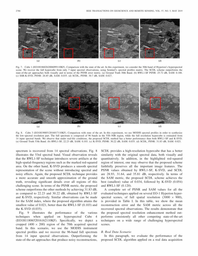
In Fig. 7, we compare the performance of SCDL with thethree state-of-the-art methods when applied on the cropped(271 × 184) area of Cube 1 (EO1H1860262006099110KF).In this experiment, we use Sentinel’s spectral profiles in
order to downsample the high-spectral resolution hyperspectraldata, and thus, we recover the full spectrum, composed of96 spectral bands, from only 7 input spectral observations.We observe that the RWL1-SF and the K-SVD techniquesare not able to reconstruct significant features such as theroad areas at the top of the scenes. One may notice thesubtle differences among the various techniques in the markedred-squared region of interest. The reweighted spatial filteringtechnique introduces severe artifacts in the reconstruction.In contrast, the K-SVD spectral superresolution approachprovides a smoother recovery compared to RWL1-SF, but notas good as the proposed SCDL scheme, which achieves thehighest accuracy with the ground truth 3-D hypercube, bothvisually and quantitatively, in terms of the attained evaluationmetrics. The PSNR values obtained by RWL1-SF, K-SVD, andSCDL are 25.72, 26.85, and 30.7 dB, respectively. In terms ofthe SAM error metric, the RWL1-SF algorithm achieves 0.188,while the K-SVD spectral superresolution approach achieves0.035. In contrast, the proposed SCDL scheme achieves aneven smaller SAM value, 0.027, indicating a higher similarityamong the reconstructed and ground truth hypercubes.
Another indicative set of reconstruction results is depictedin Fig. 8, where the performance of the various methods isevaluated on a cropped region (400 × 200) of hyperspec-tral Cube 3 (EO1H1900512016017110KF). In this experi-ment, we used MODIS spectral profiles to synthesize thelow-spectral resolution part. Hence, the full 96 spectral bands
2786 IEEE TRANSACTIONS ON GEOSCIENCE AND REMOTE SENSING, VOL. 57, NO. 5, MAY 2019
Fig. 7. Cube 1 (EO1H1860262006099110KF). Comparison with the state of the art. In this experiment, we consider the 30th band of Hyperion’s hyperspectralscene. We recover the full hypercube from only 7 input spectral observations, using Sentinel’s spectral profiles matrix. The SCDL scheme outperforms thestate-of-the-art approaches both visually and in terms of the PSNR error metric. (a) Ground Truth 30th Band. (b) RWL1-SF PSNR: 25.72 dB, SAM: 0.188.(c) SSR-K-SVD, PSNR: 26.85 dB, SAM: 0.035. (d) SCDL, PSNR: 30.7 dB, SAM: 0.027.
Fig. 8. Cube 3 (EO1H1900512016017110KF). Comparison with state of the art. In this experiment, we use MODIS spectral profiles in order to synthesizethe low-spectral resolution part. The full spectrum is composed of 96 bands in the VIS–NIR region, while the full resolution hypercube is estimated from14 input spectral bands. We observe that under real-life conditions, the proposed SCDL method has a better performance than both RWL1-SF and K-SVD.(a) Ground Truth 53th Band. (b) RWL1-SF, 22.23 dB, SAM: 0.103. (c) K-SVD, PSNR: 30.22 dB, SAM: 0.035. (d) SCDL, PSNR: 31.83 dB, SAM: 0.021.
spectrum is recovered from 14 spectral observations. Fig. 8illustrates the 53rd spectral band. Visual observation revealsthat the RWL1-SF technique introduces severe artifacts at thehigh-spatial-frequency regions such as the marked red-squaredarea. On the other hand, K-SVD produces a smooth spectralrepresentation of the scene without introducing spectral andnoisy effects. Again, the proposed SCDL technique providesa more accurate and smooth approximation of the groundtruth, revealing significant details over all regions of thischallenging scene. In terms of the PSNR metric, the proposedscheme outperforms the other methods by achieving 31.83 dB,as compared to 22.23 and 30.22 dB, obtained by RWL1-SFand K-SVD, respectively. Similar observations can be madefor the SAM index, where the proposed algorithm attains thesmallest value of 0.021, better than the RWL1-SF (0.103) andthe K-SVD (0.035).
Fig. 9 illustrates the performance of the varioustechniques when applied on hyperspectral Cube 4(EO1H1180652016162110KF). Specifically, we depict acropped (400 × 200) region of the 70th acquired spectralband. In this scenario, we use the MODIS instrumentspectral profiles and we recover the 96-band full spectrumfrom 14 input spectral observations. Outperforming thestate-of-the-art approaches that produce noisy reconstructions,
SCDL provides a high-resolution hypercube that has a bettersimilarity with the original spectral data, both visually andquantitatively. In addition, in the highlighted red-squaredregion of interest, one may observe that the proposed schemefaithfully preserves all the important image features. ThePSNR values obtained by RWL1-SF, K-SVD, and SCDLare 28.93, 31.64, and 35.81 dB, respectively. In terms ofthe SAM metric, the proposed SCDL scheme achieves thebest (smallest) value of 0.034, followed by K-SVD (0.054)and RWL1-SF (0.120).
A complete set of PSNR and SAM values for all theevaluated techniques applied on several EO-1 Hyperion hyper-spectral scenes, of full spatial resolution (3000 × 900),is provided in Table I. In this table, we show the meanreconstruction error and the SAM metric across all therecovered spectral observations. The results demonstrate thatthe proposed spectral resolution enhancement method out-performs consistently all other competing state-of-the-arttechniques on a wide range of challenging hyperspectralscenes.
B. Real Data ScenarioIn this paragraph, we evaluate the performance of the
proposed SCDL algorithm applied on a real data acquisition

FOTIADOU et al.: SPECTRAL SUPER RESOLUTION OF HYPERSPECTRAL IMAGES VIA COUPLED DICTIONARY LEARNING 2787
Fig. 9. Cube 4 (EO1H1180652016162110KF). Comparison with the state of the art. In this experiment, we reconstruct the full spectrum, composedof 96 bands in the VIS–NIR region, from 14 input spectral bands using MODIS spectral profiles matrix. The proposed scheme provides an accuratehigh-quality reconstruction of the challenging scene, both quantitatively and visually. (a) Ground Truth 70th Band. (b) RWL1-SF, 28.93 dB, SAM:0.120.(c) K-SVD, PSNR:31.64 dB, SAM:0.054. (d) SCDL, PSNR:35.81 dB, SAM:0.034.
TABLE I
QUANTITATIVE PERFORMANCE EVALUATION OF THE PROPOSED SCDL METHOD AGAINST STATE-OF-THE-ART TECHNIQUES IN
TERMS OF PSNR (IN DECIBELS) AND SAM ERROR METRICS, USING MODIS AND SENTINEL’S SPECTRAL PROFILES
Fig. 10. Real Data Scenario (North Greece Region). In this experiment, we trained the coupled dictionaries using Sentinel-2 and Landsat-8 data scannedin the same regions. During the testing phase, we consider as input 9 spectral bands of the Landsat-8 multispectral sensor, and we recover the 13 spectralobservations of the Sentinel-2 satellite. In order to verify our reconstruction, the output high-spectral resolution hypercube is compared with the ground-truthSentinel-2 cube. (c) Difference between the reconstructed 12th spectral band and the ground truth 12th band. We observe that the recovered band achieveshigh similarity with the ground truth spectral band, both visually and in terms of the evaluation metrics (PSNR and SAM). (a) Ground truth 12th band.(b) SCDL, PSNR: 39.75 dB, SAM: 0.034. (c) Difference between SCDL and Ground Truth.
case. Specifically, we considered multispectral data scanned inthe same region and extracted by the Landsat-8 OLI sensorand the Sentinel-2 sensor. The challenge is to recover the13 spectral bands of the Sentinel-2 sensor using as input9 spectral observations of the Landsat-8 sensor.
Fig. 10 demonstrates the reconstruction result for the12th spectral band of the Sentinel-2 sensor using the proposedSCDL scheme. Specifically, we illustrate the actual 12th spec-
tral band and its reconstructed version by SCDL. As we mayobserve, the achieved reconstruction has a high similarity toits corresponding ground truth spectral band, both visuallyand quantitatively in terms of the PSNR (39.75 dB) andSAM (0.034) error metrics. Fig. 10(c) illustrates the differencebetween the ground truth and the reconstructed 12th spectralband and clearly demonstrates that the proposed schemerecovers accurately the ground truth spectral observation.

2788 IEEE TRANSACTIONS ON GEOSCIENCE AND REMOTE SENSING, VOL. 57, NO. 5, MAY 2019
Fig. 11. Real Data Acquisition Scenario (North Greece Region). Comparison with state of the art. In this experiment, we depict an example of the proposedalgorithm when it is applied to real satellite data. We evaluate the reconstruction quality of the proposed SCDL scheme compared with the state of the art,in the scenario where we recover the 13 spectral bands of Sentinel-2, considering as input 9 spectral observations of Landsat-8. We observe that the proposedalgorithm outperforms the state-of-the-art techniques both in terms of the evaluation indexes and visually. In the zoomed-in view of red square regionsdepicted in the second row, we illustrate the subtle differences among the various techniques. (a) Ground truth 12th band. (b) RWL1-SF, 23.50 dB, SAM:0.224. (c) K-SVD, PSNR: 33.57 dB, SAM: 0.032. (d) SCDL, PSNR: 39.75 dB, SAM: 0.014. (e) Zoomed-in view—12th Band. (f) Zoomed-in view—RWL1-SF.(g) Zoomed-in view—SSR-K-SVD. (h) Zoomed-in view—SCDL.
Fig. 12. Real Data Scenario (North Greece Region). We provide the differences between the 12th band reconstructed by the methods and the ground truth12th spectral band of the Sentinel-2 sensor. We note that both the RWL1-SF and the K-SVD algorithms produce well-structured difference images, implyinga low-quality recovery. In contrast, the proposed technique’s difference image with respect to the ground truth denotes an accurate reconstruction of the12th spectral band. (a) Ground Truth 12th Band. (b) Difference between RWL1-SF and Ground Truth. (c) Difference between SSR-K-SVD and Ground Truth.(d) Difference between SCDL and Ground Truth.
In Fig. 11, we provide the comparison with the state-of-the-art algorithms when applied to the real data scenario. As thetesting data cube, we utilize a multispectral scene capturedby Landsat-8 on September 17, 2017. Visual observationin both the full-spatial resolution image and the croppedred-square region reveals that the RWL1-SF algorithm pro-duces noisy reconstructions with severe artifacts. Althoughthe K-SVD produces more faithful approximations of theground truth spectral information, the proposed SCDL algo-rithm synthesizes spectral observations of a higher qualitywithout introducing noise effects. Quantitatively, the proposedSCDL scheme outperforms other techniques in terms of theevaluation metrics, achieving a PSNR value of 39.75 dB,
in contrast to the RWL1-SF and the K-SVD that achieve 23.50and 33.57 dB, respectively. Similarly, in terms of the SAMerror metric, the proposed technique achieves the smallestvalue of 0.014 as compared to RWL1-SF and K-SVD thatachieve 0.224 and 0.032, respectively.
Moreover, in Fig. 12, we depict the difference betweenthe reconstruction by each algorithm and the actual 12thspectral band. As we may observe, both RWL1-SF [Fig. 12(b)]and K-SVD [Fig. 12c)] achieve reconstructions that arenoticeably different from the ground truth. In contrast,the difference image attained by our SCDL technique,as depicted in Fig. 12(d), demonstrates a high-quality recoverythat matches accurately with the ground truth 12th spectral

FOTIADOU et al.: SPECTRAL SUPER RESOLUTION OF HYPERSPECTRAL IMAGES VIA COUPLED DICTIONARY LEARNING 2789
Fig. 13. Real Data Scenario (North Greece Region). In this simulation, we illustrate the Spectral Angle Mapper (SAM) images for the comparable techniques.As we may observe, both the RWLW-SF and the K-SVD algorithms provide more degraded reconstructions, in comparison with the proposed algorithm.In addition, quantitatively, in terms of the error metric, the proposed algorithm achieves a lower SAM value, compared to the other two state-of-the-artapproaches. (a) RWSF, SAM: 0.224. (b) SSR-K-SVD, SAM: 0.032. (c) SCDL, SAM: 0.014.
Fig. 14. Hyperspectral Image Denoising. In this experiment, we provide the ground 5th spectral band of the Landsat-8, influenced by the existence of zeromean, and σ 2 = 0.05 Gaussian noise. (Left to Right) We illustrate the accurate Landsat’s-8 5th spectral band, the corresponding noisy observation, the groundtruth Sentinel’s-2 5th spectral band, and the proposed system’s reconstruction. Both in term of visual perception and quantitatively, the proposed schemeachieves a faithful reconstruction of the high-resolution data cube even on the extreme scenario when the input low-spectral resolution part is degraded bynoise. (a) Ground truth 5th Landsat’s-8 band. (b) Noisy 5th Landsat’s-8 band. (c) Ground Truth 5th Sentinel’s-2 band. (d) Recovered 5th Sentinel’s-2 band.
band. Finally, Fig. 13 demonstrates the SAM images of thecompared techniques for the North Greece Region hypercube.We observe that both visually and in terms of the SAM index,the proposed ADMM coupled dictionary learning scheme,outperforms the state-of-the-art approaches. In terms of visualperception, we may notice that our approach provides ahigh-quality SAM image of the testing hypercube, withoutintroducing noise artifacts. In constrast, both the K-SVD andRWL1-SF techniques, provide lower quality SAM images.
1) Impact on Hyperspectral Image Denoising: In this para-graph, we examine the performance of the proposed SDCLscheme on the fundamental problem of hyperspectral imagedenoising. In further detail, we considered the real data acqui-sition scenario, enhancing the spectral dimensions of Landsat-8 to the spectral resolution of the Sentinel-2 sensor. Themajor difference with the previous paragraphs is that we havealso considered the noise existence. Specifically, we assumedthat the noise distribution of the low-spectral resolution partadheres to a normal distribution, N ∼ (0, 0.05). Consequently,we have added zero-mean (μ = 0) Gaussian noise, with0.05 standard deviation ( σ 2 = 0.05), to Landsat-8’s trainingexamples. The main objective is to recover the 13 spectralbands of the Sentinel-2 sensor using as input the 9 noisyspectral observations of the Landsat-8 instrument. In order toachieve this goal, we have prepared one pair of dictionaries
that represent the low resolution and noisy part, and thecorresponding high-resolution observations.
Fig. 14 stands as an example of the proposed SCDLscheme applied on the hyperspectral image denoising problem.Specifically, we illustrate the ground truth and the noisy fifthobservation of Landsat-8 sensor, along with the synthesizedfifth spectral band of Sentinel-2. As we may notice, the pro-posed coupled dictionary learning algorithm is able to providea high-quality and spectrally superresolved data cube, fromthe noisy low-spatial and spectral resolution input.
In addition, in Fig. 15, we depict the comparison withthe state-of-the-art algorithms applied to the scenario wherethe low-spectral resolution part is influenced by the presenceof Gaussian noise. Specifically, we illustrate the 12th bandof the multispectral testing scene that was utilized in theprevious examples (i.e., Figs. 10 and 11). As we may notice,the proposed SCDL scheme outperforms both the K-SVDdictionary learning and the RWL1-SF approaches, both visu-ally but also in terms of quantitative metrics. For instance,the RWL1-SF approach achieves a SAM value of 0.398,the K-SVD reconstruction reaches the SAM value of 0.091,while the proposed SCDL algorithm achieves the smallestof 0.030. Although initial simulation results indicate thatthe proposed SCDL scheme is also capable of addressingthe hyperspectral denoising problem, a detailed analysis of

2790 IEEE TRANSACTIONS ON GEOSCIENCE AND REMOTE SENSING, VOL. 57, NO. 5, MAY 2019
Fig. 15. Impact of Hyperspectral Image Denoising (Real Data Acquisition—North Greece Region). In this simulation, we examine the reconstruction qualityof the comparable techniques when the low-resolution part of the Landsat-8 sensor is degraded by Gaussian noise. For this purpose, we trained coupleddictionaries using Sentinel-2 and noisy Landsat-8 data, scanned in the same spatial locations. To verify our recovery, the output, high-spectral resolution, anddenoised hypercube is compared with the ground truth Sentinel-2 data cube. We note that the proposed SCDL scheme outperforms the comparable literatureapproaches both in visual perception and quantitatively. Consequently, given the appropriate training, the proposed algorithm is able to confront the challengingproblem of hyperspectral image denoising. (a) 12th Sentinel’s-2 band. (b) RWL1-SF, SAM: 0.398. (c) K-SVD, SAM: 0.091. (d) SCDL, SAM: 0.030.
Fig. 16. Convergence Behavior of the proposed Dictionary LearningAlgorithm. (Left) Convergence of the two dictionaries. (Right) Convergenceof the augmented Lagrangian function. In all cases, the proposed algorithmconverges into a stationary point. (a) Convergence of Dh and D�. (b) Con-vergence of the Augmented Lagrangian L.
the denoising perspectives, including consideration of differenttypes of degradation, and subsequent comparison with state-of-the-art denoising techniques is beyond the scope of thispaper, and thus it is left as future work.
C. Convergence
In this section, we investigate the empirical convergenceof the proposed algorithm when it is applied on theMODIS to Hyperion spectral superresolution case. Specifi-cally, we examine the convergence behavior of both the high-and low-spectral resolution dictionaries, Dh, D�, as well asthe convergence of the augmented Lagrangian function L.Fig. 16 depicts the normalized reconstruction errors for thetwo dictionaries and the augmented Lagrangian function asa function of the number of iterations. We note that bothdictionaries converge after approximately 20 iterations whilethe augmented Lagrangian function needs around 60 iterationsfor convergence. We observed a similar convergence behaviorfor both the Sentinel-2 to Hyperion and the Landsat-8 toSentinel-2 spectral superresolution scenarios.
Fig. 17. Cube 5 hyperspectral scene. Sentinel to Hyperion spectral superres-olution scenario. In this simulation, we illustrate the PSNR of the proposedSCDL algorithm as a function of the number of training examples. We observethat after approximately 105 training examples, SCDL reaches a stable plateau.
D. Sensitivity to Parameters
In the following paragraphs, we investigate the impact ofthe parameters selection in our algorithm’s performance. First,we examine the number of training examples for the coupleddictionary learning procedure versus the reconstruction quality.Then, we investigate the impact of the dictionary size (numberof dictionary atoms) on the reconstruction quality. Finally,we investigate the proper selection of the sparsity regulariza-tion parameter (λ) to both the execution time of our algorithmand the reconstruction quality, in terms of PSNR.
To study the sensitivity of the proposed algorithm, we eval-uated the reconstruction performance of the coupled traineddictionaries as a function of the number of training examples.In Fig. 17, we provide the PSNR values for the reconstruc-tion of Cube 5 (EO1H1120822017023110K7) hyperspectralscene, as a function of the number of training examples.In this simulation, we use Sentinel’s spectral profiles, and thus,we synthesize the full spectrum from 7 spectral observations.Specifically, we investigated the performance of the proposed

FOTIADOU et al.: SPECTRAL SUPER RESOLUTION OF HYPERSPECTRAL IMAGES VIA COUPLED DICTIONARY LEARNING 2791
Fig. 18. Landsat-8 to Sentinel-2, real data scenario. Evaluation of thereconstruction quality in terms of the PSNR metric for 14 spectral bandindexes. The proposed SCDL scheme achieves consistently higher PSNRvalues, compared with state-of-the-art approaches.
scheme when we start from a relatively small size of trainingexamples, i.e., 0.5 × 10⁵, and we gradually increased thetraining size to 3×10⁵ examples. Results indicate that the per-formance of the SCDL method monotonically increases as afunction of the number of input training examples, as expected.However, experimentally we observed that increasing thetraining size over approximately 1.5×10⁵ examples, the PSNRreaches a stationary plateau. We note that after approximately105 training examples, SCDL achieves its highest PSNR valueof 49.50 dB. Consequently, for the spectral super-resolutionproblem, using a larger number than 105 training examplesin the coupled dictionary learning process offers a marginalimprovement to the reconstruction quality. For this reason,we fixed the training size to 105 examples.
Fig. 18 demonstrates the PSNR performance for variousspectral bands in the Landsat-8 to Sentinel-2 spectral superres-olution scenario. Note that for all spectral bands, the proposedSCDL scheme achieves higher reconstruction quality, as com-pared with the state-of-the-art techniques. On the other hand,Fig. 19 investigates the impact of the sparsity parameter λ,on both the reconstruction quality and the execution time.This experiment was implemented using the Landsat-8 toSentinel-2 spectral resolution enhancement scenario. Specif-ically, we used as a test scene, the hypercube that is depictedin Figs. 10 and 11 (North Greece Region). In order to select theproper sparsity regularization parameter for the reconstructionprocess, we have experimented with several λ values, rangingfrom 0.1 to 0.9. Specifically, we observed that for λ = 0.1our system achieves the highest reconstruction performancein terms of the PSNR error metric. As we gradually increasethe value of λ, the execution time decreases dramatically, butunfortunately, the reconstruction quality degrades. The highestPSNR value is achieved for λ = 0.1. For this value of λ,the proposed scheme reconstructs the high-spectral resolutionNorth Greece hypercube of spatial dimensions (612 × 1076)in about 2.8 min when the sparse-based RWSF-L1 approachrequires approximately 3.2 h. Consequently, the proposedSCDL scheme outperforms the state of the art both in terms
Fig. 19. (Left to Right) In this experiment, we demonstrate the impact of thesparsity regularization parameter (λ) on the reconstruction performance and onthe execution time. As the value of λ increases, the execution time decreasesand the reconstruction quality drops. For λ = 0.2, our system achieves theoptimal performance, balancing between a high-quality reconstruction, anda short execution time. (a) Sparsity parameter versus PSNR. (b) Sparsityparameter versus execution time.
Fig. 20. Reconstruction performance as a function of the dictionary size.In this experiment, we used the hypercube that is depicted in Fig. 5, andwe reconstructed the full spectrum composed of 96 spectral bands from only7 spectral observations. The best performance of 44.04 dB is achieved whenwe use 1024 dictionary atoms.
of reconstruction performance and execution time. As a result,the optimal selection of the sparsity parameter is crucialfor every sparse-based algorithm. We note that in order toachieve a fair comparison with the other two sparse-basedalgorithms (KSVD and RWSF-L1), we used the same sparseregularization term.
Finally, in Fig. 20, we demonstrate the impact of the dic-tionary size on the reconstruction performance. In this exper-iment, we utilized the hypercube that is depicted in Fig. 5,and thus, we reconstructed the full spectrum composed of96 spectral bands from only 7 spectral observations. Specif-ically, for a fixed sparsity regularization parameter, λ = 0.2,we have investigated the impact of using different dictionarysizes consisting of 512, 1024, 2048, and 4096 atoms. It isimportant to note that as we increase the number of dictionaryatoms (>1024), the reconstruction quality decreases. However,in these cases as well, the proposed recovery outperforms thestate of the art. The results indicate that the optimal reconstruc-tion performance is achieved when we use 1024 dictionary

2792 IEEE TRANSACTIONS ON GEOSCIENCE AND REMOTE SENSING, VOL. 57, NO. 5, MAY 2019
Fig. 21. SCDL recovered 20th AVIRIS Cuprite band, along with the ground truth 20th spectral band, and the absolute difference. We observe that theproposed technique’s difference image with respect to the ground truth denotes an accurate reconstruction of the 20th spectral band. (a) Ground Truth 20th Band.(b) SCDL Recovered 20th Band. (c) Difference between SCDL and Ground Truth.
atoms. Similar behavior was observed for all investigatedspectral resolution enhancement scenarios.
E. Spectral Coupled Dictionary Learning for HyperspectralImage Understanding
In the following paragraphs, we examine the impact of theproposed spectral superresolution framework on the funda-mental understanding process of hyperspectral unmixing.
Separating a remote sensing image into its elementarycomponents is crucial for multiple applications, includingprecision agriculture and weather and climate forecastingamong others [3]. Consequently, spectral unmixing providesa well-organized mapping of the pure materials that existin the raw data, by identifying the spectral signatures ofthese materials (i.e., endmembers) along with their relativecontributions (i.e., abundances). The endmembers are assumedto represent the pure materials that are depicted on the hyper-spectral scene, while the abundances represent the amount ofeach endmember that is presented in the pixel.
In order to investigate the hyperspectral unmixingperformance after applying the proposed spectral superreso-lution technique, we exploited a novel linear spectral unmix-ing algorithm, namely: fast unmixing algorithm (FUN) [69].According to the FUN algorithm, each captured pixel in ahyperspectral scene can be represented as a linear combina-tion between a definite number of endmembers weighted byan abundance factor. The specific technique provides effec-tively and with low computational complexity simultaneousextraction of the endmembers along with their abundances,by exploiting a modified Gram-Schmidt technique.
Regarding the evaluation setup, we have experimented withthe Cuprite scene acquired by the AVIRIS hyperspectralinstrument [70]. The specific hyperspectral scene has beenwidely utilized for both unmixing and classification purposes.In order to demonstrate that the proposed spectral superresolu-tion architecture provides an improvement in the hyperspectralunmixing problem, we adhered to the following experimentalscenario: first, we enhanced the spectral dimension of theCuprite scene using the proposed SCDL scheme, and then,we applied the FUN algorithm for the extraction of theendmembers and abundances. The number of reconstructed
endmembers for both the ground truth Cuprite, and thereconstructed from the degraded input, was 12. As a result,we evaluated the unmixing performance in the scenarios whenwe have the high-spectral versus the low-spectral resolutionhypercubes.
In greater detail, the high-resolution data cube wascreated by removing the noisy (B1-B2 and B221-B224), andwater vapor absorption B104-B113 and B148-B167 spectralbands, resulting into 188 spectral observations. For the con-struction of the low-resolution counterpart, we consideredthe spectral response functions of the Landsat-8 satellite.In order to provide the correspondence between the twoinstruments, we constructed the spectral profiles matrix byfinding their overlapping wavelength values. Specifically,the overlapping spectral bands among the two instrumentsare: (B8, B10, B21, B24, B31, B54, B133, B188). The spec-tral calibration data for the AVIRIS acquisition scenario forma matrix of size 188 × 8. Consequently, we reconstruct the188 high-resolution bands of AVIRIS from only 8 spectralobservations of Landsat-8 instrument.
Regarding the dictionary training phase, we preparedone pair of dictionaries corresponding to the low (8-bands) and high (188-bands) feature spaces. In addition,we utilized 5 training hypercubes from which 50.000 train-ing hyperpixels were randomly extracted. The number ofselected dictionary atoms was set to 512, while the pro-posed SCDL scheme converged into approximately 30 iter-ations. Quantitatively, the proposed SCDL scheme recon-structs the Cuprite hyperspectral scene, achieving a PSNRvalue of 44.41 dB, and a SAM error metric of 0.0368.In Fig. 21, we provide the recovered 20th spectral band ofAVIRIS Cuprite scene, using the proposed SCDL scheme,the ground truth 20th spectral and their absolute difference.As we may observe, the proposed SCDL scheme also corre-sponds with high efficiency in the specific scenario of spectraldegradation.
Concluding, in Fig. 22, we evaluate the unmixing per-formance by comparing the extracted abundancies using theSCDL superresolved hypercubes versus the abundances thatwere synthesized directly from the low-spectral resolutionCuprite hypercube. As a baseline, we utilize the 12 pub-

FOTIADOU et al.: SPECTRAL SUPER RESOLUTION OF HYPERSPECTRAL IMAGES VIA COUPLED DICTIONARY LEARNING 2793
Fig. 22. Unmxing results of the AVIRIS Cuprite hyperspectral scene. Specifically, we illustrate the abundance maps for the extracted #3, #5, and#6 endmembers. (Top to Bottom) In the first row, we depict the ground abundance maps, while in the second row, the unmixing results from the low-resolutionCuprite hypercube are presented. Finally, in the third row, we illustrate the unmixing results from the enhanced Cuprite hypercube. As we may notice,the reconstructed abundances using as input the proposed superresolved hypercube, the present high similarity with the accurate, ground truth abundances.Consequently, the proposed SCDL scheme is able to facilitate the crucial problem of hyperspectral image unmixing. (a) Ground Truth Endmember #3.(b) Ground Truth Endmember #5. (c) Ground Truth Endmember #6. (d) Endmember #3 from Low Resolution. (e) Endmember #5 from Low Resolution.(f) Endmember #6 from Low Resolution. (g) Endmember #3 from SCDL. (h) Endmember #5 from SCDL. (i) Endmember #6 from SCDL.
licly available Cuprite ground truth abundancies [70]. In allcases, we observe that the estimated abundances using thesynthesized high-spectral resolution SCDL hypercube providean accurate reconstruction of the ground truth abundancies.Consequently, the proposed SCDL recovery provides a high-quality, superresolved data cube, able to facilitate the hyper-spectral unmixing procedure.
VII. CONCLUSION
In this paper, we proposed a novel spectral superresolu-tion architecture for multispectral and hyperspectral imagery,employing the mathematical framework of sparse represen-
tations through a coupled dictionary learning algorithm forencoding the relations between high- and low-spectral reso-lution scenes. To achieve this goal, an efficient formulationwas proposed based on the alternating direction method ofmultipliers. Experimental results on both synthetic and realremote sensing data support our claim that high-quality recon-struction of multispectral and hyperspectral data is obtainedusing our method. In addition, the proposed spectral superres-olution algorithm is able to provide vital facilitation in sub-sequent hyperspectral image understanding techniques, suchas spectral unmixing and classification. Finally, our schemecan be extended to handle arbitrary low-to-high resolutionenhancements by simple modifications of the joint dictionary

2794 IEEE TRANSACTIONS ON GEOSCIENCE AND REMOTE SENSING, VOL. 57, NO. 5, MAY 2019
learning process, and it offers the capability of addressingadditional sources of HSI image degradation.
APPENDIX
Derivations of the individual subproblems for theSCDL-ADMM-based dictionary learning scheme, as describedin Section IV.
1) Subproblem Wh
W�h = argmin
Wh
L
⇔ ∇Wh
1
2�Sh − DhWh�2
2 + �Y1, P − Wh�
+ �Y3, Wh − W��c1
2�P − Wh�2
2
+c3
2�Wh − W��2
2
�
= −DTh · (Sh − DhWh) − Y1 + Y3 − c1
· (P − Wh) + c3 · (Wh − W�).
Setting
∇WhL = 0
⇔ −Dh · Sh + DTh · Dh · Wh − Y1 + Y3 − c1
· P + c1 · Wh + c3 · Wh − c3 · W� = 0
⇔ �DT
h · Dh + c1 · I + c3 · I� · Wh
= DTh · Sh + Y1 − Y3 + c1 · P + c3 · W�
⇔ W�h = �
DTh · Dh + c1 · I + c3 · I
�−1
× �DT
h · Sh + Y1 − Y3 + c1 · P + c3 · W�
�.
2) Subproblem W�
W� = argminW�
L
⇔ ∇Wl
1
2· �S� − D�W��2
2 + �Y2, Q − W��
+ �Y3, Wh −W��+ c2
2�Q−W��2
2
+ c3
2�Wh − W��2
2
�
= −DT� · (S� − D�W�)−Y2
− Y3 − c2 · (Q − W�) + c3 · (Wh − W�).
Setting
∇W�L = 0 ⇔ −D� · S� + DT� · D� · W� − Y2 − Y3 − c2
· Q + c2 · W� − c3 · Wh
= 0 ⇔ �DT
� · D� + c2 · I + c3 · I�
· W� = DT� · S� + Y2 + Y3 + c2 · Q + c3
· Wh −c3 · W� ⇔W��
= �DT
� · D� + c2 · I + c3 · I�−1
· �DT� · S� + Y2 + Y3 + c2 · Q + c3 · Wh
�.
3) Subproblem P
P� = argminP
L
⇔ ∇P
�λh�P�1 + �Y1, P − Wh� + c1
2�P − Wh�2
2
�.
a) For P > 0
∇PL = λh · I + c1 · (P − Wh) + Y1
. Setting ∇PL = 0
P� = Wh − 1
c1· (Y1 + λh · I )
b) For P < 0
∇PL = −λh · I + c1 · (P − Wh) + Y1
Setting ∇PL = 0
P� = Wh − 1
c1· (Y1 − λh · I )
Combining
P > 0 ⇔ Wh − 1
c1· Y1 >
1
c1· λh · I
P > 0 ⇔ Wh − 1
c1· Y1 > − 1
c1· λh · I
we have Wh − 1
c1· Y1
≤ 1
c1· λh · I.
Consequently
P� = Sλh
Wh − Y1
c1
�
where Sλh denotes the soft-thresholding operator,defined as
Sλh (x) = sign(x) · max(|x | − λh , 0).
4) Subproblem Q
Q� = argminQ
L ⇔ .
a) For Q > 0
∇QL = λ� · I + Y2 + c2 · (Q − W�).
Setting ∇QL = 0
Q = W� − 1
c2· (Y2 + λ� · I )
b) For Q < 0
∇QL = λ� · I + Y2 + c2 · (Q − W�)
Setting ∇QL = 0
Q = W� − 1
c2· (Y2 − λ� · I )
Combining
Q > 0 ⇔ W� − 1
c2· Y2 >
1
c2· λ� · I
Q > 0 ⇔ W� − 1
c2· Y2 > − 1
c2· λ� · I
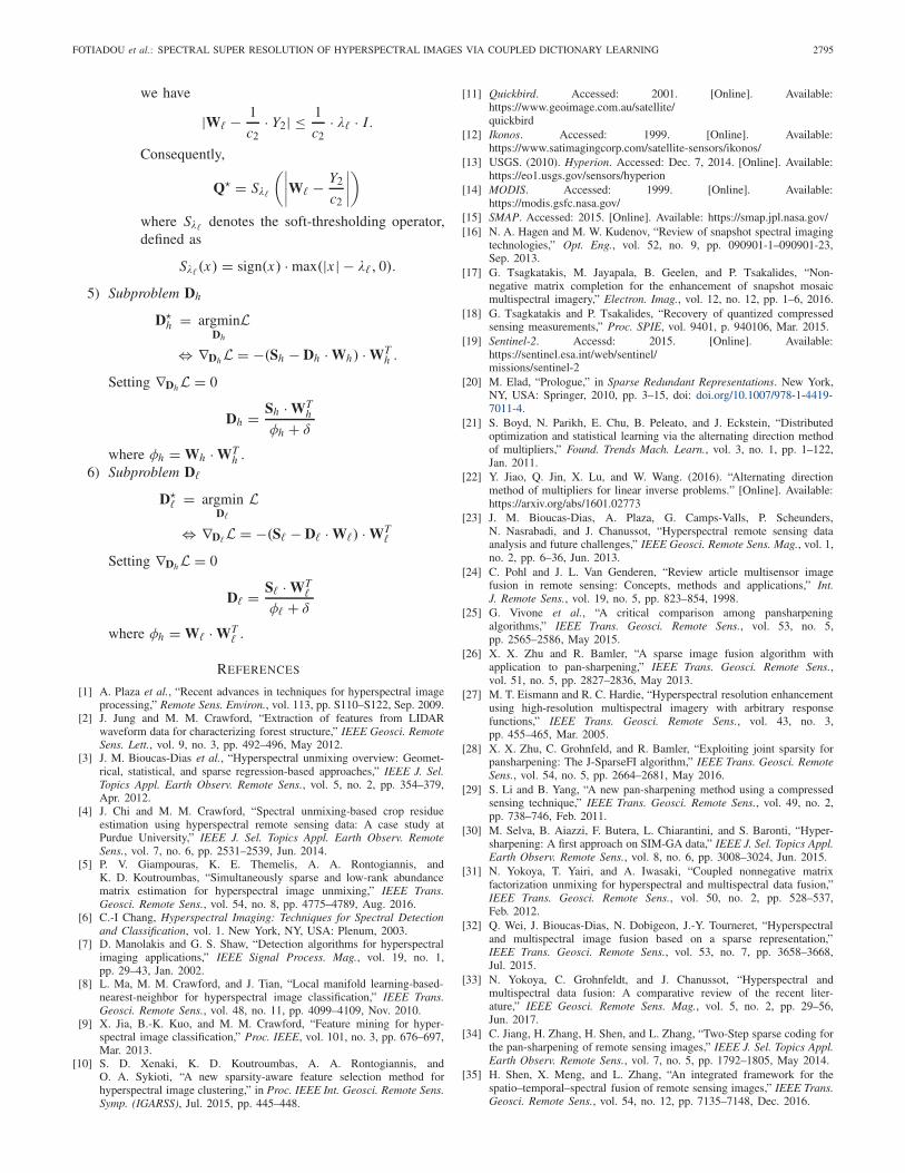
FOTIADOU et al.: SPECTRAL SUPER RESOLUTION OF HYPERSPECTRAL IMAGES VIA COUPLED DICTIONARY LEARNING 2795
we have
|W� − 1
c2· Y2| ≤ 1
c2· λ� · I.
Consequently,
Q� = Sλ�
W� − Y2
c2
�
where Sλ� denotes the soft-thresholding operator,defined as
Sλ�(x) = sign(x) · max(|x | − λ�, 0).
5) Subproblem Dh
D�h = argmin
Dh
L
⇔ ∇DhL = −(Sh − Dh · Wh) · WTh .
Setting ∇DhL = 0
Dh = Sh · WTh
φh + δ
where φh = Wh · WTh .
6) Subproblem D�
D�� = argmin
D�
L
⇔ ∇D�L = −(S� − D� · W�) · WT�
Setting ∇DhL = 0
D� = S� · WT�
φ� + δ
where φh = W� · WT� .
REFERENCES
[1] A. Plaza et al., “Recent advances in techniques for hyperspectral imageprocessing,” Remote Sens. Environ., vol. 113, pp. S110–S122, Sep. 2009.
[2] J. Jung and M. M. Crawford, “Extraction of features from LIDARwaveform data for characterizing forest structure,” IEEE Geosci. RemoteSens. Lett., vol. 9, no. 3, pp. 492–496, May 2012.
[3] J. M. Bioucas-Dias et al., “Hyperspectral unmixing overview: Geomet-rical, statistical, and sparse regression-based approaches,” IEEE J. Sel.Topics Appl. Earth Observ. Remote Sens., vol. 5, no. 2, pp. 354–379,Apr. 2012.
[4] J. Chi and M. M. Crawford, “Spectral unmixing-based crop residueestimation using hyperspectral remote sensing data: A case study atPurdue University,” IEEE J. Sel. Topics Appl. Earth Observ. RemoteSens., vol. 7, no. 6, pp. 2531–2539, Jun. 2014.
[5] P. V. Giampouras, K. E. Themelis, A. A. Rontogiannis, andK. D. Koutroumbas, “Simultaneously sparse and low-rank abundancematrix estimation for hyperspectral image unmixing,” IEEE Trans.Geosci. Remote Sens., vol. 54, no. 8, pp. 4775–4789, Aug. 2016.
[6] C.-I Chang, Hyperspectral Imaging: Techniques for Spectral Detectionand Classification, vol. 1. New York, NY, USA: Plenum, 2003.
[7] D. Manolakis and G. S. Shaw, “Detection algorithms for hyperspectralimaging applications,” IEEE Signal Process. Mag., vol. 19, no. 1,pp. 29–43, Jan. 2002.
[8] L. Ma, M. M. Crawford, and J. Tian, “Local manifold learning-based-nearest-neighbor for hyperspectral image classification,” IEEE Trans.Geosci. Remote Sens., vol. 48, no. 11, pp. 4099–4109, Nov. 2010.
[9] X. Jia, B.-K. Kuo, and M. M. Crawford, “Feature mining for hyper-spectral image classification,” Proc. IEEE, vol. 101, no. 3, pp. 676–697,Mar. 2013.
[10] S. D. Xenaki, K. D. Koutroumbas, A. A. Rontogiannis, andO. A. Sykioti, “A new sparsity-aware feature selection method forhyperspectral image clustering,” in Proc. IEEE Int. Geosci. Remote Sens.Symp. (IGARSS), Jul. 2015, pp. 445–448.
[11] Quickbird. Accessed: 2001. [Online]. Available:https://www.geoimage.com.au/satellite/quickbird
[12] Ikonos. Accessed: 1999. [Online]. Available:https://www.satimagingcorp.com/satellite-sensors/ikonos/
[13] USGS. (2010). Hyperion. Accessed: Dec. 7, 2014. [Online]. Available:https://eo1.usgs.gov/sensors/hyperion
[14] MODIS. Accessed: 1999. [Online]. Available:https://modis.gsfc.nasa.gov/
[15] SMAP. Accessed: 2015. [Online]. Available: https://smap.jpl.nasa.gov/[16] N. A. Hagen and M. W. Kudenov, “Review of snapshot spectral imaging
technologies,” Opt. Eng., vol. 52, no. 9, pp. 090901-1–090901-23,Sep. 2013.
[17] G. Tsagkatakis, M. Jayapala, B. Geelen, and P. Tsakalides, “Non-negative matrix completion for the enhancement of snapshot mosaicmultispectral imagery,” Electron. Imag., vol. 12, no. 12, pp. 1–6, 2016.
[18] G. Tsagkatakis and P. Tsakalides, “Recovery of quantized compressedsensing measurements,” Proc. SPIE, vol. 9401, p. 940106, Mar. 2015.
[19] Sentinel-2. Accessd: 2015. [Online]. Available:https://sentinel.esa.int/web/sentinel/missions/sentinel-2
[20] M. Elad, “Prologue,” in Sparse Redundant Representations. New York,NY, USA: Springer, 2010, pp. 3–15, doi: doi.org/10.1007/978-1-4419-7011-4.
[21] S. Boyd, N. Parikh, E. Chu, B. Peleato, and J. Eckstein, “Distributedoptimization and statistical learning via the alternating direction methodof multipliers,” Found. Trends Mach. Learn., vol. 3, no. 1, pp. 1–122,Jan. 2011.
[22] Y. Jiao, Q. Jin, X. Lu, and W. Wang. (2016). “Alternating directionmethod of multipliers for linear inverse problems.” [Online]. Available:https://arxiv.org/abs/1601.02773
[23] J. M. Bioucas-Dias, A. Plaza, G. Camps-Valls, P. Scheunders,N. Nasrabadi, and J. Chanussot, “Hyperspectral remote sensing dataanalysis and future challenges,” IEEE Geosci. Remote Sens. Mag., vol. 1,no. 2, pp. 6–36, Jun. 2013.
[24] C. Pohl and J. L. Van Genderen, “Review article multisensor imagefusion in remote sensing: Concepts, methods and applications,” Int.J. Remote Sens., vol. 19, no. 5, pp. 823–854, 1998.
[25] G. Vivone et al., “A critical comparison among pansharpeningalgorithms,” IEEE Trans. Geosci. Remote Sens., vol. 53, no. 5,pp. 2565–2586, May 2015.
[26] X. X. Zhu and R. Bamler, “A sparse image fusion algorithm withapplication to pan-sharpening,” IEEE Trans. Geosci. Remote Sens.,vol. 51, no. 5, pp. 2827–2836, May 2013.
[27] M. T. Eismann and R. C. Hardie, “Hyperspectral resolution enhancementusing high-resolution multispectral imagery with arbitrary responsefunctions,” IEEE Trans. Geosci. Remote Sens., vol. 43, no. 3,pp. 455–465, Mar. 2005.
[28] X. X. Zhu, C. Grohnfeld, and R. Bamler, “Exploiting joint sparsity forpansharpening: The J-SparseFI algorithm,” IEEE Trans. Geosci. RemoteSens., vol. 54, no. 5, pp. 2664–2681, May 2016.
[29] S. Li and B. Yang, “A new pan-sharpening method using a compressedsensing technique,” IEEE Trans. Geosci. Remote Sens., vol. 49, no. 2,pp. 738–746, Feb. 2011.
[30] M. Selva, B. Aiazzi, F. Butera, L. Chiarantini, and S. Baronti, “Hyper-sharpening: A first approach on SIM-GA data,” IEEE J. Sel. Topics Appl.Earth Observ. Remote Sens., vol. 8, no. 6, pp. 3008–3024, Jun. 2015.
[31] N. Yokoya, T. Yairi, and A. Iwasaki, “Coupled nonnegative matrixfactorization unmixing for hyperspectral and multispectral data fusion,”IEEE Trans. Geosci. Remote Sens., vol. 50, no. 2, pp. 528–537,Feb. 2012.
[32] Q. Wei, J. Bioucas-Dias, N. Dobigeon, J.-Y. Tourneret, “Hyperspectraland multispectral image fusion based on a sparse representation,”IEEE Trans. Geosci. Remote Sens., vol. 53, no. 7, pp. 3658–3668,Jul. 2015.
[33] N. Yokoya, C. Grohnfeldt, and J. Chanussot, “Hyperspectral andmultispectral data fusion: A comparative review of the recent liter-ature,” IEEE Geosci. Remote Sens. Mag., vol. 5, no. 2, pp. 29–56,Jun. 2017.
[34] C. Jiang, H. Zhang, H. Shen, and L. Zhang, “Two-Step sparse coding forthe pan-sharpening of remote sensing images,” IEEE J. Sel. Topics Appl.Earth Observ. Remote Sens., vol. 7, no. 5, pp. 1792–1805, May 2014.
[35] H. Shen, X. Meng, and L. Zhang, “An integrated framework for thespatio–temporal–spectral fusion of remote sensing images,” IEEE Trans.Geosci. Remote Sens., vol. 54, no. 12, pp. 7135–7148, Dec. 2016.

2796 IEEE TRANSACTIONS ON GEOSCIENCE AND REMOTE SENSING, VOL. 57, NO. 5, MAY 2019
[36] K. Zhang, M. Wang, and S. Yang, “Multispectral and hyperspectralimage fusion based on group spectral embedding and low-rank factoriza-tion,” IEEE Trans. Geosci. Remote Sens., vol. 55, no. 3, pp. 1363–1371,Mar. 2017.
[37] Y. Wei, Q. Yuan, H. Shen, and L. Zhang, “Boosting the accuracy ofmultispectral image pansharpening by learning a deep residual network,”IEEE Geosci. Remote Sens. Lett., vol. 14, no. 10, pp. 1795–1799,Oct. 2017.
[38] X. Kang, S. Li, and J. A. Benediktsson, “Pansharpening with mat-ting model,” IEEE Trans. Geosci. Remote Sens., vol. 52, no. 8,pp. 5088–5099, Aug. 2014.
[39] X. He, L. Condat, J. M. Bioucas-Dias, J. Chanussot, and J. Xia, “A newpansharpening method based on spatial and spectral sparsity priors,”IEEE Trans. Image Process., vol. 23, no. 9, pp. 4160–4174, Sep. 2014.
[40] M. Guo, H. Zhang, J. Li, L. Zhang, and H. Shen, “An online coupled dic-tionary learning approach for remote sensing image fusion,” IEEE J. Sel.Topics Appl. Earth Observ. Remote Sens., vol. 7, no. 4, pp. 1284–1294,Apr. 2014.
[41] S. Galliani, C. Lanaras, D. Marmanis, E. Baltsavias, and K. Schindler.(2017). “Learned spectral super-resolution.” [Online]. Available: https://arxiv.org/abs/1703.09470
[42] J. Hu, Y. Li, and W. Xie, “Hyperspectral image super-resolution byspectral difference learning and spatial error correction,” IEEE Geosci.Remote Sens. Lett., vol. 14, no. 10, pp. 1825–1829, Oct. 2017.
[43] S. Mei, X. Yuan, J. Ji, Y. Zhang, S. Wan, and Q. Du, “Hyperspectralimage spatial super-resolution via 3D full convolutional neural network,”Remote Sens., vol. 9, no. 11, p. 1139, 2017.
[44] J. Bieniarz, R. Müller, X. X. Zhu, and P. Reinartz, “Hyperspectral imageresolution enhancement based on joint sparsity spectral unmixing,” inProc. IEEE Geosci. Remote Sens. Symp., Jul. 2014, pp. 2645–2648.
[45] Y. Zhao, C. Yi, J. Yang, and J. C.-W. Chan, “Coupled hyperspectralsuper-resolution and unmixing,” in Proc. IEEE Geosci. Remote Sens.Symp., Jul. 2014, pp. 2641–2644.
[46] A. Ertürk, M. K. Güllü, D. Çesmeci, D. Gerçek, and S. Ertürk, “Spatialresolution enhancement of hyperspectral images using unmixing andbinary particle swarm optimization,” IEEE Geosci. Remote Sens. Lett.,vol. 11, no. 12, pp. 2100–2104, Dec. 2014.
[47] W. Dong et al., “Hyperspectral image super-resolution via non-negativestructured sparse representation,” IEEE Trans. Image Process., vol. 25,no. 5, pp. 2337–2352, May 2016.
[48] N. Akhtar, F. Shafait, and A. Mian, “Bayesian sparse representation forhyperspectral image super resolution,” in Proc. IEEE Conf. Comput. Vis.Pattern Recognit., Jun. 2015, pp. 3631–3640.
[49] H. Yin, S. Li, and L. Fang, “Simultaneous image fusion and super-resolution using sparse representation,” Inf. Fusion, vol. 14, no. 3,pp. 229–240, 2013.
[50] J. Yang, J. Wright, T. S. Huang, and Y. Ma, “Image super-resolutionvia sparse representation,” IEEE Trans. Image Process., vol. 19, no. 11,pp. 2861–2873, Nov. 2010.
[51] J. Yang, Z. Wang, Z. Lin, X. Shu, and T. Huang, “Bilevel sparse codingfor coupled feature spaces,” in Proc. IEEE Conf. Comput. Vis. PatternRecognit. (CVPR), Jun. 2012, pp. 2360–2367.
[52] L. He, H. Qi, and R. Zaretzki, “Beta process joint dictionary learningfor coupled feature spaces with application to single image super-resolution,” in Proc. IEEE Conf. Comput. Vis. Pattern Recognit.,Jun. 2013, pp. 345–352.
[53] K. Fotiadou, G. Tsagkatakis, B. Moraes, F. B. Abdalla, and P. Tsakalides,“Denoising galaxy spectra with coupled dictionary learning,” in Proc.25th Eur. Signal Process. Conf. (EUSIPCO), Aug. 2017, pp. 498–502.
[54] A. S. Charles, B. A. Olshausen, and C. J. Rozell, “Learning sparse codesfor hyperspectral imagery,” IEEE J. Sel. Topics Signal Process., vol. 5,no. 5, pp. 963–978, Sep. 2011.
[55] A. S. Charles and C. J. Rozell, “Spectral superresolution of hyperspectralimagery using reweighted �1 spatial filtering,” IEEE Geosci. RemoteSens. Lett., vol. 11, no. 3, pp. 602–606, Mar. 2014.
[56] A. S. Charles, C. J. Rozell, and N. B. Tufillaro, “Sparsity based spectralsuper-resolution and applications to ocean water color,” in Proc. IGARSSTech. Abstract, 2014, pp. 1–4.
[57] K. Fotiadou, G. Tsagkatakis, and P. Tsakalides, “Multi-source imageenhancement via coupled dictionary learning,” in Proc. Signal Process.Adapt. Sparse Struct. Represent. Workshop (SPARS), 2017, pp. 1–2.
[58] K. Fotiadou, G. Tsagkatakis, and P. Tsakalides, “Spectral resolutionenhancement of hyperspectral images via sparse representations,” inProc. Comput. Imag., IS&T Int. Symp. Electron. Imag., 2016, pp. 1–6.
[59] L. Yuan, J. Sun, L. Quan, and H.-Y. Shum, “Image deblurring withblurred/noisy image pairs,” ACM Trans. Graph, vol. 26, no. 3, p. 1,Jul. 2007.
[60] K. Fotiadou, G. Tsagkatakis, and P. Tsakalides, “Low light imageenhancement via sparse representations,” in Proc. Int. Conf. Image Anal.Recognit. Springer, 2014, pp. 84–93.
[61] M. Aharon, M. Elad, and A. Bruckstein, “K-SVD: An algorithm fordesigning overcomplete dictionaries for sparse representation,” IEEETrans. Signal Process., vol. 54, no. 11, pp. 4311–4322, Nov. 2006.
[62] Y. Li, X. Xie, and Z. Yang, “Alternating direction method of multipliersfor solving dictionary learning models,” Commun. Math. Statist., vol. 3,no. 1, pp. 37–55, 2015.
[63] M. Hong, Z.-Q. Luo, and M. Razaviyayn, “Convergence analysis ofalternating direction method of multipliers for a family of nonconvexproblems,” SIAM J. Optim., vol. 26, no. 1, pp. 337–364, 2016.
[64] Landsat-8. Accessed: 2013. [Online]. Available:https://landsat.usgs.gov/landsat-8
[65] A. K. Singh, H. V. Kumar, G. R. Kadambi, J. K. Kishore, J. Shuttle-worth, and J. Manikandan, “Quality metrics evaluation of hyperspectralimages,” in Proc. Int. Arch. Photogramm., Remote Sens. Spatial Inf. Sci.,vol. 40, no. 8, pp. 1221–1226, 2014.
[66] R. H. Yuhas, A. F. Goetz, and J. W. Boardman, “Discrimination amongsemi-arid landscape endmembers using the spectral angle mapper (SAM)algorithm,” Tech. Rep., 1992.
[67] O. A. De Carvalho and P. R. Meneses, “Spectral correlation mapper(SCM): An improvement on the spectral angle mapper (SAM),” in Proc.Summaries 9th JPL Airborne Earth Sci. Workshop, JPL Publication,vol. 9. Pasadena, CA, USA: JPL Publication, 2000.
[68] J. D. O’Sullivan, P. R. Hoy, and H. N. Rutt, “An extended spectral anglemap for hyperspectral and multispectral imaging,” in Proc. CLEO, LaserSci. Photon. Appl., May 2011, Paper CMG2.
[69] R. Guerra, L. Santos, S. López, and R. Sarmiento, “A new fast algo-rithm for linearly unmixing hyperspectral images,” IEEE Trans. Geosci.Remote Sens., vol. 53, no. 12, pp. 6752–6765, Dec. 2015.
[70] Aviris. Accessed: 2012. [Online]. Available: https://aviris.jpl.nasa.gov/
Konstantina Fotiadou received the B.Sc. degreein applied mathematics from the Department ofApplied Mathematics, University of Crete (UoC),Crete, Greece, and the M.Sc. degree in computer sci-ence from the Computer Science Department, UoC,in 2011 and 2014, respectively. She is currentlypursuing the Ph.D. degree in computer science fromthe Department of Computer Science, UoC, underthe supervision of Prof. P. Tsakalides.
Since 2012, she has been a Research Assistantwith the Signal Processing Laboratory, Institute of
Computer Science, Foundation for Research & Technology–Hellas, Heraklion,Greece. She is involved in PHySIS and DEDALE European Projects. Herresearch interests include machine learning techniques for image process-ing and computational photography applications, and hyperspectral imageenhancement techniques.

FOTIADOU et al.: SPECTRAL SUPER RESOLUTION OF HYPERSPECTRAL IMAGES VIA COUPLED DICTIONARY LEARNING 2797
Grigorios Tsagkatakis received the Diploma andM.S. degrees in electronics and computer engi-neering from the Technical University of Crete,Chania, Greece, in 2005 and 2007, respectively,and the Ph.D. degree in imaging science from theRochester Institute of Technology, Rochester, NY,USA, in 2011.
From 2011 to 2013, he was a Marie CuriePost-Doctoral Fellow with the Institute of Com-puter Science (ICS), Foundation for Research &Technology–Hellas (FORTH), Heraklion, Greece.
He is currently a Research Associate with the Signal Processing Laboratory,FORTH–ICS. He has been involved in various European projects, includ-ing H2020 PHySIS and DEDALE, FP7 CS-ORION & HYDROBIONETS,FP6 OPTAG, and industry-funded projects by leading companies includingKodak, Rochester, and Cisco, San Jose, CA, USA. He has coauthored morethan 30 peer-reviewed conferences, journals, and book chapters in the areasof signal and image processing, computer vision, and machine learning.
Dr. Tsagkatakis was a recipient of the Best Paper Award in the WesternNew York Image Processing Workshop in 2010 for his paper—A Frameworkfor Object Class Recognition with No Visual Examples.
Panagiotis Tsakalides received the Diploma degreein electrical engineering from the Aristotle Univer-sity of Thessaloniki, Thessaloniki, Greece, in 1990,and the Ph.D. degree in electrical engineering fromthe University of Southern California, Los Angeles,CA, USA, in 1995.
He was involved in transferring research and inter-acting with the industry and projects related to theSmall Business Innovation Research and TechnologyTransfer programs of the U.S. Government. He wasthe Project Coordinator or Co-Principal Investigator
in eight European Commission projects and nine national projects, totallymore than 4.5 million euro in actual funding for the University of Crete,Heraklion, Greece, and Institute of Computer Science (ICS), Foundation forResearch & Technology–Hellas (FORTH), Heraklion. From 2010 to 2014,he was a Coordinator of the 1.3 Million euro FP7 MC-IAPP CS-ORIONProject, conducting research on compressed sensing for remote imaging in aer-ial and terrestrial surveillance. He is currently a Coordinator of the 1 Millioneuro H2020 COMPET Project PHySIS, conducting research on sparse signalprocessing technologies for hyperspectral systems. He is currently a Professorand the Chairman of the Computer Science Department, University of Crete,and the Head of the Signal Processing Laboratory, FORTH–ICS, Heraklion.He has a strong commitment in inspiring young researchers, having supervised4 Ph.D. and 16 M.Sc. students and 8 post-doctoral fellows. His researchinterests include statistical signal processing with emphasis in non-Gaussianestimation and detection theory, sparse representations, and applications insensor networks, audio, imaging, and multimedia systems. He has coauthoredover 150 technical publications in these areas, including 30 journal papers.