Spectral residual method without gradient

information for solving large-scale nonlinear

systems of equations

William La Cruz ∗ Jose Mario Martınez † Marcos Raydan ‡

May 26, 2005

Abstract

A fully derivative-free spectral residual method for solving large-scale nonlinear systems of equations is presented. It uses in a system-atic way the residual vector as a search direction, a spectral steplengththat produces a nonmonotone process and a globalization strategy thatallows for this nonmonotone behavior. The global convergence analysisof the combined scheme is presented. An extensive set of numericalexperiments that indicate that the new combination is competitive andfrequently better than well-known Newton-Krylov methods for large-scale problems is also presented.

Keywords: nonlinear systems, spectral gradient method, nonmono-tone line search, Newton-Krylov methods.

1 Introduction

We introduce a derivative-free nonmonotone iterative method for solving thenonlinear system of equations

F (x) = 0, (1)∗Departamento de Electronica, Computacion y Control, Facultad de Ingenierıa, Uni-

versidad Central de Venezuela, Caracas, Venezuela. This author was supported by AgendaPetroleo UCV-PROJECT 97-003769. E-mail: wlacruz@elecrisc.ing.ucv.ve

†Department of Applied Mathematics, IMECC-UNICAMP, University of Camp-inas, CP 6065, 13081-970 Campinas SP, Brazil. This author was supported byPRONEX-Optimization 76.79.1008-00, FAPESP (Grant 2001-04597-4), CNPq and FAEP-UNICAMP. E-mail: martinez@ime.unicamp.br

‡Departamento de Computacion, Facultad de Ciencias, Universidad Central deVenezuela, Apartado 47002, Caracas 1041-A, Venezuela. This author was supported byAgenda Petroleo UCV-PROJECT 97-003769. E-mail: mraydan@kuaimare.ciens.ucv.ve

1

where F : IRn → IRn is a continuously differentiable mapping. We areinterested in large-scale systems for which the Jacobian of F is not availableor requires a prohibitive amount of storage.

Recently, La Cruz and Raydan [17] introduced the Spectral Algorithmfor Nonlinear Equations (SANE) for solving (1). SANE uses in a systematicway the residual ±F (xk) as search direction. The first trial point at eachiteration is xk − σkF (xk) where σk is a spectral coefficient. Global conver-gence is guaranteed by means of a variation of the nonmonotone strategy ofGrippo, Lampariello and Lucidi [13]. This approach requires descent direc-tions with respect to the squared norm of the residual. As a consequence,the computation of a directional derivative, or a very good approximationof it, is necessary at every iteration.

The spectral coefficient is an appropriate Rayleigh quotient with respectto a secant approximation of the Jacobian. Spectral gradient methods forminimization were originated in the Barzilai-Borwein paper [1]. The proper-ties of their method for general quadratic functions were elucidated in [23].Further analysis of spectral gradient methods can be found in [8, 10, 24]among others. For a review containing the more recent advances on spec-tral choices of the steplength for minimization problems, see [11].

In this paper we introduce a new nonmonotone line-search techniquethat can be associated to the same search directions and the same initialsteplengths as the SANE algorithm. In other words, the first trial point ateach iteration will be the same as in SANE, but the line-search strategy isdifferent. The main consequence is that, in the new approach, directionalderivatives are not required at all.

We also present an extensive set of numerical experiments that indicatethat the new method is competitive and sometimes better than the SANEalgorithm. We recall that, in [17], SANE was in turn compared favorablywith several Newton-Krylov methods (see, e.g., [2, 6, 7]). Therefore, thenew algorithm represents an encouraging low-cost scheme for solving (1).

Notation.

• J(x) will denote the Jacobian matrix of F computed at x.

• For all x ∈ IRn we denote g(x) = 2J(x)tF (x) = ∇‖F (x)‖22.• The set of natural numbers will be denoted IN = {0, 1, 2, . . .}.• If {zk}k∈IN is a sequence and K = {k1, k2, k3, . . .} is an infinite se-

quence of natural numbers such that ki < kj if i < j, we denote:

limk∈K

zk = limj→∞

zkj.

2

• The symbol ‖ · ‖ will always denote the Euclidian norm.

• B(x, ε) will denote the open ball with center x and radius ε. That is:

B(x, ε) = {z ∈ IRn | ‖z − x‖ < ε}.

2 The new nonmonotone line-search strategy

The best known nonmonotone line-search technique for unconstrained op-timization was introduced by Grippo, Lampariello and Lucidi [13]. It hasbeen used to globalize the spectral gradient method [24] and some of itsextensions for convex constrained optimization [3, 4] and nonlinear systemsof equations [17]. Different nonmonotone line-search techniques, associatedto Newton and quasi-Newton strategies, have been proposed for solving (1).See [12, 18]. Li and Fukushima [18] presented an interesting idea that avoidsthe necessity of descent directions to guarantee that each iteration is welldefined. Let us briefly describe the Grippo-Lampariello-Lucidi (GLL) andthe Li-Fukushima (LF) schemes.

The GLL condition can be written as follows:

f(xk + αkdk) ≤ max0≤j≤M−1

f(xk−j) + γαk∇f(xk)tdk,

where M is a nonnegative integer, 0 < γ < 1 and f is a merit function suchthat f(x) = 0 if and only if ‖F (x)‖ = 0.

The LF condition can be written as follows:

‖F (xk + αkdk)‖ ≤ (1 + ηk)‖F (xk)‖ − γα2k‖dk‖22,

where∑

k ηk ≤ η <∞.It follows that if ∇f(xk)tdk < 0, then the GLL condition is satisfied

for αk sufficiently close to zero and we can compute a steplength αk byusing a finite backtracking process. However, when ∇f(xk)tdk = 0, theexistence of αk satisfying the GLL condition is not guaranteed. Moreover,when dk = ±F (xk), ∇f(xk)tdk could be close to zero or zero, and thenstagnation or breakdown might occur during the backtracking process.

One possible remedy is to use the LF condition. This condition does notneed the computation of J(xk)dk. Moreover, it is satisfied, if αk is smallenough, independently of the choice of dk. However, since ηk is usuallyvery small when k is large, the Li-Fukushima strategy generally imposes analmost monotone behavior of the merit function when xk is close to a solu-tion. This is not a good feature when one uses spectral gradient or spectralresidual steps because, in these cases, the pure undamped methods (where

3

αk = 1 for all k), although generally effective, are usually highly nonmono-tone even in the neighborhood of an isolated solution. The reason for this isnot completely understood but the analogy with the behavior of the spec-tral gradient (or Barzilai-Borwein) method for minimizing convex quadraticsmay be useful. See [23]. In the quadratic case the spectral gradient methoddoes not need line-search strategies for being globally convergent, but thefunctional values do not decrease monotonically at all. Therefore, impos-ing any kind of monotonicity is not convenient. Many authors, includingFletcher [11], pointed out the necessity of avoiding monotonicity require-ments in the spectral framework as much as possible.

In this work we combine and extend the GLL and LF conditions to pro-duce a robust nonmonotone line-search globalization strategy that somehowtakes into account the advantages of both schemes. Roughly speaking thenew descent condition can be written as:

f(xk+1) ≤ max0≤j≤M−1

f(xk−j) + ηk − γα2kf(xk). (2)

The GLL term max0≤j≤M−1 f(xk−j) is responsible for the sufficientlynonmonotone behavior of f(xk) even when k is large. On the other hand,the presence of ηk > 0 guarantees that all the iterations are well definedand the forcing term −γα2

kf(xk) provides the arguments for proving globalconvergence.

We would like to mention that a similar extension that also combines theGLL with the LF conditions was presented and briefly discussed in the finalremarks of [17]. However, it was neither analyzed nor tested. The presentwork was motivated by the need of studying the theoretical and practicalproperties of this globalization technique.

3 Model algorithm and convergence

We assume that F : IRn → IRn has continuous partial derivatives. Letnexp ∈ {1, 2}. Define

f(x) = ‖F (x)‖nexp for all x ∈ IRn.

Assume that {ηk} is a sequence such that ηk > 0 for all k ∈ IN and

∞∑k=0

ηk = η <∞. (3)

Assume that 0 < γ < 1 and 0 < σmin < σmax <∞. Let M be a positiveinteger. Let τmin, τmax be such that 0 < τmin < τmax < 1, and let x0 ∈ IRn

be an arbitrary initial point.

4

We now present the DF-SANE algorithm.

Algorithm DF-SANE (Derivative-free SANE).

Step 0.Set k ← 0.

Step 1.

• Choose σk such that |σk| ∈ [σmin, σmax] (the spectral coefficient)

• Compute fk = max{f(xk), . . . , f(xmax{0,k−M+1})}.• Set d← −σkF (xk).

• Set α+ ← 1, α− ← 1.

Step 2.If f(xk + α+d) ≤ fk + ηk − γα2

+f(xk) thenDefine dk = d, αk = α+, xk+1 = xk + αkdk

else if f(xk − α−d) ≤ fk + ηk − γα2−f(xk) thenDefine dk = −d, αk = α−, xk+1 = xk + αkdk

elsechoose α+new ∈ [τminα+, τmaxα+], α−new ∈ [τminα−, τmaxα−],replace α+ ← α+new, α− ← α−new

and go to Step 2.

Step 3.If F (xk+1) = 0, terminate the execution of the algorithm. Else, set

k ← k + 1 and go to Step 1.

Remark. As we will see later, the coefficient σk will be chosen to be anapproximation of the quotient ‖F (xk)‖2

〈J(xk)F (xk),F (xk)〉 . This quotient may be pos-itive or negative (or even null).

Proposition 1. The iteration is well defined.Proof. Since ηk > 0, after a finite number of reductions of α+ the condition

f(xk + α+d) ≤ fk + ηk − γα2+f(xk)

necessarily holds. �

In the rest of this section we will prove several convergence results:

5

1. There exists an infinite sequence of indices K ⊂ IN such that at everylimit point of the subsequence {xk}k∈K , the gradient of ‖F (x)‖2 isorthogonal to the residual F (x). Therefore, if ‖F (x)‖ has boundedlevel sets, there exists a limit point x∗ of {xk}k∈IN such that

〈J(x∗)F (x∗), F (x∗)〉 = 0.

2. If some limit point of {xk}k∈IN is a solution of (1), then every limitpoint is a solution;

3. If a limit point x∗ of {xk}k∈IN is an isolated solution then the wholesequence converges to x∗.

4. If the initial point x0 is close enough to some strongly isolated solu-tion x∗ then the whole sequence converges to x∗.

Only the first result was proved for the original SANE algorithm [17]although it is easy to realize that the other ones hold for SANE as well.When breakdown does not occur, under standard assumptions, Newton-Krylov methods have stronger local convergence results in the sense thatlinear or, sometimes, superlinear convergence can be proved.

Before we proceed with the convergence analysis, we need some prelim-inary definitions (see [5]). Define V0 = f(x0) and

Vk = max{f(x(k−1)M+1), . . . , f(xkM )}

for all k = 1, 2, . . .Let ν(k) ∈ {(k − 1)M + 1, . . . , kM} be such that, for all k = 1, 2, . . .,

f(xν(k)) = Vk.

Clearly,

f(xkM+1) ≤ max{f(x(k−1)M+1), . . . , f(xkM)}+ ηkM − γα2kMf(xkM)

= Vk + ηkM − γα2kMf(xkM)

≤ Vk + ηkM ,

f(xkM+2) ≤ max{Vk, f(xkM+1)}+ ηkM+1 − γα2kM+1f(xkM+1)

≤ Vk + ηkM + ηkM+1 − γα2kM+1f(xkM+1)

≤ Vk + ηkM + ηkM+1

and so on.

6

Therefore, by an inductive argument,

f(xkM+�) ≤ Vk +�−1∑j=0

ηkM+j − γα2kM+�−1f(xkM+�−1) (4)

for all � = 0, 1, 2, . . . ,M . Moreover,

f(xkM+�) ≤ Vk +�−1∑j=0

ηkM+j ∀ k, � ∈ IN. (5)

But ν(k + 1) ∈ {kM + 1, . . . , kM + M}, thus, by (4),

Vk+1 = f(xν(k+1)) ≤ Vk +M−1∑j=0

ηkM+j − γα2ν(k+1)−1f(xν(k+1)−1)

= f(xν(k)) +M−1∑j=0

ηkM+j − γα2ν(k+1)−1f(xν(k+1)−1). (6)

Using (4), (5) and (6) we can prove the following propositions:

Proposition 2. For all k, � ∈ IN ,

f(xkM+�) ≤ f(xν(k)) +∞∑

i=ν(k)

ηi ≤ f(xν(k)) + η. (7)

Proof. Straightforward, using (5). �

Proposition 3.

limk→∞

α2ν(k)−1f(xν(k)−1) = 0.

Proof. Write the inequalities (6) for k = 1, 2, . . . , L. Observe that f(xν(k+1))occurs on the left-hand side of the k-th inequality and also on the right-handside of the k + 1-st inequality. Adding the L inequalities, we get:

f(xν(L+1)) ≤ f(xν(1)) +(L+1)M−1∑

j=M

ηj − γL∑

j=1

α2ν(j+1)−1f(xν(j+1)−1).

Therefore, for all L = 1, 2, . . ., we obtain:

γ∑L

j=1 α2ν(j+1)−1f(xν(j+1)−1) ≤ f(xν(1)) +

∑(L+1)M−1j=M ηj − f(xν(L+1))

≤ f(xν(1)) +∑(L+1)M−1

j=M ηj

≤ f(xν(1)) + η

7

So, the series∑∞

j=1 α2ν(j+1)−1f(xν(j+1)−1) is convergent. This implies the

desired result. �

From now on we define:

K = {ν(1) − 1, ν(2) − 1, ν(3)− 1, . . .}. (8)

andK+ = {ν(1), ν(2), ν(3), . . .}. (9)

Observe that

ν(j + 1) ≤ ν(j) + 2M − 1 for all j = 1, 2, . . . (10)

In Theorem 1 we prove that, at every limit point x∗ of the subsequence{xk}k∈K one necessarily has that 〈J(x∗)F (x∗), F (x∗)〉 = 〈F (x∗), g(x∗)〉 = 0.In other words the gradient of ‖F (x)‖2 at x∗ is orthogonal to the resid-ual F (x∗).

Theorem 1. Assume that {xk}k∈IN is generated by the DF-SANE algo-rithm. Then, every limit point x∗ of {xk}k∈K satisfies

〈F (x∗), J(x∗)tF (x∗)〉 = 0. (11)

Proof. By Proposition 3 we have that

limk∈K

α2kf(xk) = 0. (12)

Let x∗ be a limit point of {xk}k∈K . Let K1 ⊂ K be an infinite sequence ofindices such that

limk∈K1

xk = x∗.

Then, by (12),lim

k∈K1

α2kf(xk) = 0. (13)

If {αk}k∈K1 does not tend to zero, there exists an infinite sequence ofindices K2 ⊂ K1 such that αk is bounded away from zero for k ∈ K2. Then,by (13),

limk∈K2

f(xk) = 0.

Since f is continuous and limk∈K2 xk = x∗ this implies that f(x∗) = 0. ThusF (x∗) = 0 and (11) holds.

So, we only need to analyze the case

limk∈K1

αk = 0. (14)

8

At Step 2 of Algorithm DF-SANE one tests the inequality

f(xk + α+d) ≤ fk + ηk − γα2+f(xk). (15)

If (15) does not hold, the inequality

f(xk − α−d) ≤ fk + ηk − γα2−f(xk) (16)

is tested.The first trial steps at (15)-(16) are α+ = α− = 1. By (14), there exists

k0 ∈ K1 such that αk < 1 for all k ≥ k0, k ∈ K1. For those iterations of theDF-SANE algorithm, the line search was not immediately successful and α+

and α− were adapted at least once. Suppose that in DF-SANE step k (i.e.,the step which generates xk+1) α+ and α− were adapted mk times in theline search process (i.e., the inequalities (15) and (16) were violated bothtogether mk times). Let α+

k and α−k be the values of α+ and α− respectively

in the last unsucessful line search step (the last step at which (15) and (16)were violated together) in DF-SANE step k. Because of the choice of α+new

and α−new at Step 2 of the DF-SANE algorithm we have that

αk ≥ τmkmin

for all k ≥ k0, k ∈ K1 and so, by (14), So, by (14),

limk∈K1

mk =∞.

But, again by the choice of α+new and α−new,

α+k ≤ τmk−1

max

andα−

k ≤ τmk−1max .

Therefore, since τmax < 1,

limk∈K1

α+k = lim

k∈K1

α−k = 0.

Clearly, since d = −σkF (xk), the fact that (15) and (16) are not satisfiedby α+

k and α−k respectively implies that

f(xk − α+k σkF (xk)) > fk + ηk − γ(α+

k )2f(xk) (17)

andf(xk + α−

k σkF (xk)) > fk + ηk − γ(α−k )2f(xk) (18)

for all k ∈ K1, k ≥ k0.

9

The inequality (17) implies that

f(xk − α+k σkF (xk)) > f(xk)− γ(α+

k )2f(xk).

So,f(xk − α+

k σkF (xk))− f(xk) ≥ −γ(α+k )2f(xk).

By Proposition 2, f(xk) ≤ c ≡ f(x0) + η for all k ∈ IN . Thus,

f(xk − α+k σkF (xk))− f(xk) ≥ −cγ(α+

k )2. (19)

• Let us consider first the case nexp = 2. Then, by (19),

‖F (xk − α+k σkF (xk))‖2 − ‖F (xk)‖2 ≥ −cγ(α+

k )2.

• Now consider the case nexp = 1. The subsequence {xk}k∈K1 is con-vergent and, therefore, bounded. Since ‖F (xk)‖, α+

k and σk are alsobounded, we have that {xk−α+

k σkF (xk)}k∈K1 is bounded. So, by thecontinuity of F , there exists c1 > 0 such that

‖F (xk − α+k σkF (xk))‖+ ‖F (xk)‖ ≤ c1 for all k ∈ K1.

Multiplying both sides of (19) by ‖F (xk − α+k σkF (xk))‖ + ‖F (xk)‖,

we obtain that

‖F (xk − α+k σkF (xk))‖2 − ‖F (xk)‖2 ≥ −cc1γ(α+

k )2.

Setting C = c if nexp = 2 and C = cc1 if nexp = 1, we obtain that

‖F (xk − α+k σkF (xk))‖2 − ‖F (xk)‖2 ≥ −Cγ(α+

k )2.

So,‖F (xk − α+

k σkF (xk))‖2 − ‖F (xk)‖2α+

k

≥ −Cγα+k .

By the Mean Value Theorem, there exists ξk ∈ [0, 1] such that

〈g(xk − ξkα+k σkF (xk)),−σkF (xk)〉 ≥ −Cγα+

k .

Therefore,

σk〈g(xk − ξkα+k σkF (xk)),−F (xk)〉 ≥ −Cγα+

k . (20)

By the definition of the algorithm we have that σk > 0 for infinitely manyindices or σk < 0 for infinitely many indices. If σk > 0 for infinitely manyindices k ∈ K2 ⊂ K1, the inequality (20) implies that, for k ∈ K2, k ≥ k0,

〈g(xk − ξkα+k σkF (xk)), F (xk)〉 ≤ Cγα+

k

σk≤ Cγα+

k

σmin. (21)

10

Using (18) and proceeding in the same way, we obtain that, for k ∈ K2, k ≥k0,

〈g(xk + ξ′kα−k σkF (xk)), F (xk)〉 ≥ −Cγα−

k

σk≥ −Cγα−

k

σmin(22)

for some ξ′k ∈ [0, 1].Since α+

k → 0, α−k → 0, and ‖σkF (xk)‖ is bounded, taking limits in (21)

and (22), we obtain that

〈g(x∗), F (x∗)〉 = 0. (23)

If σk < 0 for infinitely many indices, proceeding in an analogous way, wealso deduce (23). Thus, the thesis is proved. �

Corollary 1. Assume that {xk}k∈IN is generated by the DF-SANE algo-rithm, x∗ is a limit point of {xk}k∈K and for all v ∈ IRn, v �= 0,

〈J(x∗)v, v〉 �= 0.

Then, F (x∗) = 0.

Proof. Straightforward, using Theorem 1. �

As usually, we say that a matrix A ∈ IRn×n is positive-definite if 〈Av, v〉 >0 for all v ∈ IRn, v �= 0. If J(x) is positive-definite for all x ∈ IRn we saythat the mapping F is strictly monotone. If F is strictly monotone or −Fis strictly monotone, we say that the mapping F is strict. If a mapping isstrict and admits a solution, its solution must be unique. See [22], Chapter 5.

Corollary 2. Assume that {xk}k∈IN is generated by the DF-SANE al-gorithm and the mapping F is strict. Then, every bounded subsequenceof {xk}k∈K converges to the solution of (1).

Proof. Straightforward, using Corollary 1. �

Corollary 3. Assume that {xk}k∈IN is generated by the DF-SANE algo-rithm, the mapping F is strict and the level set {x ∈ IRn | f(x) ≤ f(x0)+η}is bounded. Then, {xk}k∈K converges to the solution of (1). �

Proof. Straightforward, using Corollary 2.

So far, we proved that at every limit point of {xk}k∈K the gradient of‖F (x∗)‖2 is orthogonal to the residual F (x∗). The case in which there ex-ists a limit point of {xk}k∈IN at which F (x∗) = 0 deserves further analysis.

11

The theorem below shows that, when such a limit point exists, then all thelimit points of the sequence generated by the algorithm are solutions of thenonlinear system.

Theorem 2. Assume that the sequence {xk}k∈IN is generated by the DF-SANE Algorithm and that there exists a limit point x∗ of {xk}k∈IN such thatF (x∗) = 0. Then

limk→∞

F (xk) = 0.

Consequently, F (x) vanishes at every limit point of {xk}k∈IN .

Proof. Let K1 be an infinite subset of IN such that

limk∈K1

xk = x∗

andF (x∗) = 0. (24)

Then,lim

k∈K1

F (xk) = 0.

Therefore, since xk+1 = xk ± αkσkF (xk) and |αkσk| ≤ σmax for all k ∈ IN ,

limk∈K1

‖xk+1 − xk‖ = 0.

So,lim

k∈K1

xk+1 = x∗.

Proceeding by induction, we may prove that for all fixed � ∈ {0, 1, 2, . . . , 2M−1},

limk∈K1

xk+� = x∗. (25)

Now, by (10), for all k ∈ K1, we can choose µ(k) ∈ {0, 1, . . . , 2M − 1} suchthat

k + µ(k) ∈ K+. (26)

Moreover, at least one value of µ(k) must be repeated infinitely many times.So, there exists �0 ∈ {0, 1, . . . , 2M − 1} such that µ(k) = �0 for infinitelymany indices k ∈ K1. Consider

K2 = {k + µ(k) | k ∈ K1 and µ(k) = �0}.By (25) and (26) we have that K2 ⊂ K+ and

limk∈K2

xk = x∗.

12

Then, by (24),lim

k∈K2

F (xk) = 0.

Since K2 ⊂ K+, there exists an infinite subsequence of indices J1 such that

limj∈J1

xν(j) = x∗ (27)

andlimj∈J1

f(xν(j)) = limj∈J1

Vj = 0. (28)

Let us write J1 = {j1, j2, j3, . . .}, where j1 < j2 < j3 < . . . and limi→∞ ji =∞. By (28) we have that

limi→∞

Vji = 0. (29)

Now, by (6) we have that for all j ∈ IN , j > ji,

Vj ≤ Vji +∞∑

�=Mji

η�.

Therefore,

supj≥ji

Vj ≤ Vji +∞∑

�=Mji

η�. (30)

By the summability of ηk,

limi→∞

∞∑�=Mji

η� = 0.

Then, by (29), taking limits on both sides of (30), we get:

limi→∞

supj≥ji

Vj = 0.

Thus,lim

j→∞Vj = 0.

By the definition of Vj this implies that

limk→∞

‖F (xk)‖ = limk→∞

f(xk) = 0, (31)

as we wanted to prove.The second part of the proof is straightforward: if x is a limit point of

{xk}k∈IN there exists a subsequence {xk}k∈K3 that converges to x. By (31)and the continuity of F we have that

F (x) = limk∈K3

F (xk) = 0.

13

This completes de proof. �

Now we prove two theorems of local convergence type. Theorem 3 saysthat if an isolated solution is a limit point of {xk}, then the whole sequencexk converges to this solution.

Theorem 3. Assume that the sequence {xk}k∈IN is generated by the DF-SANE algorithm and that there exists a limit point x∗ of the sequence {xk}k∈IN

such that F (x∗) = 0. Moreover, assume that there exists δ > 0 such thatF (x) �= 0 whenever 0 < ‖x− x∗‖ ≤ δ. Then, limk→∞ xk = x∗.

Proof. By Theorem 2 we have that

limk→∞

F (xk) = 0.

Therefore, since αk and σk are bounded,

limk→∞

‖xk+1 − xk‖ = 0.

Thus, there exists k1 ∈ IN such that

‖xk+1 − xk‖ ≤ δ/2 for all k ≥ k1. (32)

Consider the set

S = {x ∈ IRn | δ

2≤ ‖x− x∗‖ ≤ δ}.

By hypothesis, S does not contain any solution of F (x) = 0. But, byTheorem 2, all the limit points of {xk}k∈IN are solutions of (1). Therefore,S does not contain any limit point of {xk}k∈IN . Thus, since S is compact,it cannot contain infinitely many iterates xk. This implies that there existsk2 ∈ IN such that

xk /∈ S for all k ≥ k2. (33)

Let k3 ≥ max{k1, k2} be such that

‖xk3 − x∗‖ ≤ δ/2.

By (32), we have:

‖xk3+1 − x∗‖ ≤ ‖xk3 − x∗‖+ ‖xk3+1 − xk3‖ ≤ δ.

But, by (33), xk3+1 /∈ S, therefore, we have that

‖xk3+1 − x∗‖ ≤ δ/2.

14

Continuing this argument inductively we have that

‖xk − x∗‖ ≤ δ/2 for all k ≥ k3. (34)

This implies that all the limit points x of the sequence {xk}k∈IN are suchthat

‖x− x∗‖ ≤ δ/2.

By Theorem 2, F (x) = 0 at every limit point x and, by the hypothesis ofthis theorem, the set defined by 0 < ‖x − x∗‖ ≤ δ/2 does not contain solu-tions of (1). Therefore, this set does not contain limit points. So, the onlylimit point x that satisfies ‖x− x∗‖ ≤ δ/2 is x∗. So, by (34), the sequenceconverges to x∗ as we wanted to prove. �

Theorem 4 is our second local convergence theorem. For proving it weneed a new definition and a technical lemma. We say that x∗ ∈ IRn is astrongly isolated solution of (1) if F (x∗) = 0 and there exists ε > 0 such that

0 < ‖x− x∗‖ ≤ ε⇒ 〈J(x)F (x), F (x)〉 �= 0.

That is, in a reduced neighborhood of a strongly isolated solution the resid-ual F (x) is not orthogonal to the gradient J(x)tF (x). Theorem 4 says that,if the initial point x0 is close enough to a strongly isolated solution x∗, thenthe sequence {xk} converges to x∗. Observe that this cannot be deducedfrom Theorem 3 and, moreover, Theorem 3 cannot be deduced from thisresult either, since the strong isolation assumption is not necessary to provethat theorem.

Lemma 1. Assume that F (x∗) = 0, k ∈ IN and δ > 0. Then, there existsδ(k) ∈ (0, δ] such that for any possible initial point x0 such that ‖x0−x∗‖ <δ(k), the k-th iterate computed by the DF-SANE algorithm will satisfy

‖xk− x∗‖ < δ.

(The value of δ(k) does not depend on the particular choice of σk at Step 1or on the choices of α+new, α−new at Step 2.)

Proof. We proceed by induction. If k = 0 the result is trivial with δ(k) = δ.Assume that it is true for k = 0, 1, . . . , k and let us prove it for k + 1. Letδ > 0. Observe that, by the definition of the algorithm,

‖xk+1− x

k‖ ≤ σmax‖F (x

k)‖. (35)

Since F is continuous and F (x∗) = 0, there exists

δ′ ∈ (0, δ/2) (36)

15

such that‖x− x∗‖ < δ′ ⇒ ‖F (x)‖ < δ/2σmax.

So, by (35),‖x

k− x∗‖ < δ′ ⇒ ‖x

k+1− x

k‖ < δ/2. (37)

But, by the inductive hypothesis, there exists δ ∈ (0, δ′] such that

‖x0 − x∗‖ < δ ⇒ ‖xk− x∗‖ < δ′. (38)

By (36), (37) and (38), if ‖x0 − x∗‖ < δ, we have:

‖xk+1− x∗‖ ≤ ‖xk

− x∗‖+ ‖xk+1− x

k‖ < δ′ + δ/2 < δ.

This completes the proof. �

Theorem 4. Assume that x∗ is a strongly isolated solution of F (x) = 0.Then, there exists δ > 0 such that

‖x0 − x∗‖ < δ ⇒ limk→∞

xk = x∗,

where {xk}k∈IN is the sequence generated by the DF-SANE algorithm for thestarting point x0.

Proof. Let ε > 0 be such that

0 < ‖x− x∗‖ ≤ ε⇒ 〈J(x)F (x), F (x)〉 �= 0. (39)

Since |σkαk| ≤ σmax, ‖xk+1 − xk‖ ≤ |σkαk|‖F (xk)‖ and F (x∗) = 0, thecontinuity of F implies that there exists

ε1 ∈ (0, ε/2]

such that

‖xk−x∗‖ ≤ ε1 ⇒ ‖F (xk)−F (x∗)‖ = ‖F (xk)‖ ≤ ε

2σmax⇒ ‖xk+1−xk‖ < ε/2.

(40)Define

Cε = {x ∈ IRn | ε1 ≤ ‖x− x∗‖ ≤ ε}.Since Cε is compact and f is continuous, f has a minimum in Cε. So, thereexists x ∈ Cε, β > 0, such that

β ≡ f(x) ≤ f(x) for all x ∈ Cε. (41)

16

Since f is continuous, the set {x ∈ B(x∗, ε1/2) | f(x) < β/2} is an openneighborhood of x∗. Therefore, there exists δ ∈ (0, ε1/2) such that

‖x− x∗‖ < δ ⇒ f(x) < β/2. (42)

Let m ≥ 1 be such that

∞∑i=(m−1)M+1

ηi < β/2.

By Proposition 2, writing k0 = mM , we have that

f(xk) ≤ Vm +∞∑

i=(m−1)M+1

ηi < Vm + β/2 (43)

for all k ≥ k0.Now, apply Lemma 1 for k = (m − 1)M + 1, . . . ,mM with δ given by

(42). It turns out that there exist δ(m−1)M+1, . . . , δmM such that

‖x0 − x∗‖ < δ(m−1)M+j ⇒ ‖x(m−1)M+j − x∗‖ ≤ δ < ε1, j = 1, 2, . . . ,M.

So, taking δ = min{δ(m−1)M+1, . . . , δmM}, we have that:

‖x0 − x∗‖ < δ ⇒ ‖x(m−1)M+j − x∗‖ ≤ δ < ε1, j = 1, 2, . . . ,M. (44)

In particular, since k0 = mM ,

‖x0 − x∗‖ < δ ⇒ ‖xk0 − x∗‖ ≤ δ < ε1. (45)

By (42) and (44), f(x(m−1)M+j) < β/2 and thus Vm < β/2. So, by (43),

f(xk) < β for all k ≥ k0. (46)

Let us prove by induction that, choosing ‖x0 − x∗‖ < δ,

‖xk0+j − x∗‖ < ε1 (47)

for all j ∈ IN . By (45), we have that (47) is true for j = 0.Assume, as inductive hypothesis, that, for some j ≥ 1,

‖xk0+j−1 − x∗‖ < ε1.

Since ε1 ≤ ε/2, then‖xk0+j−1 − x∗‖ < ε/2.

17

But, by (40),

‖xk0+j − x∗‖ ≤ ‖xk0+j−1 − x∗‖+ ‖xk0+j − xk0+j−1‖ < ε/2 + ε/2 = ε. (48)

Since, by (46), f(xk0+j) < β, (41) and (48) imply that ‖xk0+j − x∗‖ < ε1.This completes the inductive proof.

So, {xk}k≥k0 ⊂ B(x∗, ε1). Therefore, all the limit points x of {xk}k∈IN

are such that ‖x−x∗‖ ≤ ε1 < ε. But, by (39) and Theorem 1, the only possi-ble limit point is x∗. Therefore, limk→∞ xk = x∗ as we wanted to prove. �

Corollary 4. Assume that x∗ is a solution of F (x) = 0 and assume thatJ(x∗) is either positive definite or negative definite. Then, there exists δ > 0such that

‖x0 − x∗‖ < δ ⇒ limk→∞

xk = x∗

with {xk}k∈IN the sequence generated by the DF-SANE algorithm for thestarting point x0.

Proof. Using the continuity of J we obtain that x∗ is strongly isolated.Then, the thesis follows from Theorem 4. �

4 Numerical results

We implemented DF-SANE with the following parameters: nexp = 2,σmin = 10−10, σmax = 1010, σ0 = 1, τmin = 0.1, τmax = 0.5, γ = 10−4,M = 10, ηk = ‖F (x0)‖/(1 + k)2 for all k ∈ IN .

The spectral steplength was computed by the formula

σk =〈sk, sk〉〈sk, yk〉 ,

where sk = xk+1 − xk and yk = F (xk+1) − F (xk). Observe that yk =[∫ 10 J(xk + tsk)dt]sk, so σk is the inverse of the Rayleigh quotient

〈[∫ 10 J(xk + tsk)dt]sk, sk〉

〈sk, sk〉 .

However, if |σk| �∈ [σmin, σmax], we replace the spectral coefficient by

σk =

1 if ‖F (xk)‖ > 1,‖F (xk)‖−1 if 10−5 ≤ ‖F (xk)‖ ≤ 1,

105 if ‖F (xk)‖ < 10−5.

18

Since we use big values for σmax and 1/σmin this replacement rarelyoccurs. In the few cases in which the replacement is necessary the first trialpoint is xk−F (xk) if ‖F (xk‖ ≥ 1. If 10−5 ≤ ‖F (xk)‖ ≤ 1 the step σk is suchthat the distance between xk and the first trial point is equal to 1. When‖F (xk)‖ < 1 we prefer to allow the distance between xk and the trial pointto be smaller, choosing for σk the fixed value 10−5.

For choosing α+new and α−new at Step 2, we proceed as follows. Givenα+ > 0, we take α+new > 0 as

α+new =

τminα+ if αt < τminα+,τmaxα+ if αt > τmaxα+,αt otherwise,

where

αt =α2

+f(xk)f(xk + α+d) + (2α+ − 1)f(xk)

.

We use similar formulae for choosing α−new as a function of α−, f(xk) andf(xk − α−d). This parabolic model is similar to the one described in [15,pp.142-143], in which the Jacobian matrix at xk is replaced by the identitymatrix (see also [9]).

We also implemented SANE [17] with the following parameters: γ =10−4, ε = 10−8, σ1 = 0.1, σ2 = 0.5, α0 = 1, M = 10, and

δ =

1 if ‖F (xk)‖ > 1,‖F (xk)‖−1 if 10−5 ≤ ‖F (xk)‖ ≤ 1,

105 if ‖F (xk)‖ < 10−5.

Both in SANE and DF-SANE we stop the process when

‖F (xk)‖√n

≤ ea + er‖F (x0)‖√

n, (49)

where ea = 10−5 and er = 10−4.We ran SANE and DF-SANE using a set of large-scale test problems.

The first twenty (1-20) test problems are fully described in [17] or referencesthere in. The complete set of test problems is described in our expandedreport [16].

The numerical results are shown in Tables 1, 2, and 3. We report only onefailure, denoted by the symbol (*), when running problem 18 with n = 100.In that case, FD-SANE fails because it generates a sequence that convergesto a point x at which F (x)T g(x) = 0, but F (x) �= 0 and g(x) �= 0.

The results from Tables 1 and 2 are summarized in Table 3. In Table 3we compare the performance (number of problems for which each method

19

is a winner with respect to number of iterations, function evaluations andcomputer time) between SANE and DF-SANE. In Tables 1 and 2 we reportthe problem number and the dimension of the problem (Function(n)), thenumber of iterations (IT), the number of function evaluations (includingthe additional functional evaluations that SANE uses for approximatingdirectional derivatives) (FE), the number of backtrackings (BK), and theCPU time in seconds (T). In SANE it is necessary to evaluate the directionalderivative 〈F (xk), J(xk)tF (xk)〉 at each iteration. Since we assume that theJacobian is not easily available we use the fact that

〈F (xk), J(xk)tF (xk)〉 = 〈J(xk)F (xk), F (xk)〉and the approximation

J(xk)F (xk) ≈ F (xk + tF (xk))− F (xk)t

where t > 0 is a small parameter. Therefore, computing the approximatedirectional derivative involves an additional function evaluation (included inFE) at each iteration.

Our results indicate that the new fully derivative-free scheme DF-SANEis competitive with the SANE algorithm, which in turn is preferable quitefrequently to the Newton-Krylov methods: Newton - GMRES, Newton -BiCGSTAB, and Newton - TFQMR (see [17] for comparisons). In particular,when comparing SANE with Newton - GMRES (which was the Krylov-likemethod with the best performance in [17]) the summary results shown inTable 4 were obtained.

5 Conclusions

The algorithm presented in this paper may be considered a damped quasi-Newton method for solving nonlinear systems. See [9, 20]. The iterationsare

xk+1 = xk − αkB−1k F (xk) (50)

where the Jacobian approximation Bk has the very simple form

Bk = σkI. (51)

In most cases,

σk =〈sk, sk〉〈yk, sk〉 . (52)

Due to the simplicity of the Jacobian approximation, the method is veryeasy to implement, memory requirements are minimal and, so, its use forsolving large-scale nonlinear systems is attractive.

20

SANE DF-SANE

Function(n) IT FE BK T IT FE BK T

1( 1000) 5 10 0 .010 5 5 0 .0001(10000) 2 4 0 .060 2 2 0 .050

2( 500) 6 14 1 .010 11 11 0 .0002( 2000) 2 7 1 .010 11 11 0 .030

3( 100) 5 10 0 .010 5 5 0 .0003( 500) 1 2 0 .000 1 1 0 .010

4( 99) 130 335 69 .060 99 289 66 .0604( 999) 130 335 69 .611 101 325 71 .611

5( 9) 23 59 12 .000 42 68 12 .0005( 49) 552 1942 424 .070 732 2958 660 .130

6( 100) 2 5 1 .000 3 3 0 .0006(10000) 2 5 1 .040 3 3 0 .060

7( 100) 23 49 2 .010 23 29 2 .0007(10000) 23 49 2 .581 23 29 2 .511

8( 1000) 1 2 0 .000 1 1 0 .0008(10000) 1 2 0 .030 1 1 0 .030

9( 100) 6 12 0 .040 6 6 0 .0209( 1000) 6 12 0 3.826 6 6 0 2.063

10( 100) 1 8 1 .000 2 12 1 .00010( 500) 1 8 1 .010 2 12 1 .010

11( 99) 11 34 4 .000 17 49 7 .00011( 399) 11 34 4 .020 17 49 7 .030

12( 1000) 6 14 2 .040 30 62 12 .18012(10000) 5 12 2 .421 23 59 11 2.073

13( 100) 3 8 1 .000 3 7 1 .01013( 1000) 4 10 1 .020 4 8 1 .010

14( 2500) 11 25 1 .210 11 17 1 .16014(10000) 12 28 1 1.082 12 20 1 .871

15( 5000) 5 10 0 .060 5 5 0 .05015(15000) 5 10 0 .230 5 5 0 .180

16( 500) 14 29 1 .000 14 16 1 .01016( 2000) 16 32 0 .010 16 16 0 .010

17( 100) 9 19 1 .010 9 11 1 .00017( 1000) 7 15 1 .030 7 9 1 .030

18( 50) 24 50 2 .010 19 21 1 .00018( 100) 24 49 1 .000 * * * *

19( 1000) 5 10 0 .010 5 5 0 .01019(50000) 5 10 0 .771 5 5 0 .611

20( 100) 32 67 2 .010 40 42 1 .01020( 1000) 51 117 9 .100 44 62 5 .070

21( 399) 4 9 1 .010 5 7 1 .00021( 9999) 4 9 1 .200 5 7 1 .190

22( 1000) 1 2 0 .000 1 2 0 .00022(15000) 1 2 0 .030 1 2 0 .040

Table 1: SANE vs. DF-SANE for the first set of test problems.

21

SANE DF-SANE

Function(n) IT FE BK T IT FE BK T

23( 500) 1 10 1 .000 2 18 1 .01023(1000) 1 11 1 .000 2 20 1 .000

24( 500) 25 54 4 .030 54 109 18 .07024( 1000) 265 915 159 .951 17 25 3 .030

25( 100) 2 6 1 .000 2 6 1 .00025( 500) 3 9 1 .000 3 9 1 .000

26( 1000) 1 2 0 .000 1 1 0 .00026( 10000) 1 2 0 .020 1 1 0 .020

27( 50) 10 20 0 .260 10 10 0 .14027( 100) 11 22 0 1.072 11 11 0 .561

28( 100) 1 2 0 .000 1 1 0 .00028(1000) 1 2 0 .000 1 1 0 .000

29( 100) 1 4 1 .010 1 5 1 .00029(1000) 1 4 1 .010 1 5 1 .010

30( 99) 18 39 3 .000 11 16 2 .00030(9999) 18 39 3 .791 11 16 2 .411

31( 1000) 4 9 0 .030 6 6 0 .02031( 5000) 4 9 0 .160 6 6 0 .130

32( 500) 6 12 0 .010 6 7 0 .01032( 1000) 6 12 0 .020 6 7 0 .020

33( 1000) 3 20 2 .050 37 50 3 .12033( 5000) 3 22 1 .270 4 16 2 .230

34( 1000) 22 52 4 .110 78 155 26 .38134(5000) 12 27 1 .361 12 18 1 .280

35( 1000) 21 45 2 .180 21 27 2 .11035( 5000) 29 63 3 1.402 38 48 3 1.202

36( 1000) 21 45 2 .270 28 34 2 .21036(5000) 44 96 7 2.954 26 36 4 1.272

37( 1000) 23 49 2 .010 26 38 5 .01037(5000) 23 49 2 .140 26 38 5 .210

38( 1000) 19 40 2 .050 25 30 2 .04038(5000) 19 40 2 .320 25 30 2 .340

39(1000) 55 126 13 .160 14 20 1 .03039(5000) 55 126 13 1.041 14 20 1 .210

40(1000) 1 2 0 .000 1 1 0 .00040(5000) 1 2 0 .020 1 1 0 .020

41( 500) 7 15 1 .010 7 9 1 .01041(1000) 2 5 1 .010 3 3 0 .000

42( 1000) 110 268 45 .190 173 412 85 .33042( 5000) 110 268 45 1.392 173 412 85 2.654

43( 100) 80 175 11 .010 86 108 9 .01043( 500) 488 1704 348 .601 586 1162 193 .451

44( 1000) 2 4 0 .020 4 4 0 .03044(5000) 2 4 0 .100 3 3 0 .090

Table 2: SANE vs. DF-SANE for the second set of test problems.

22

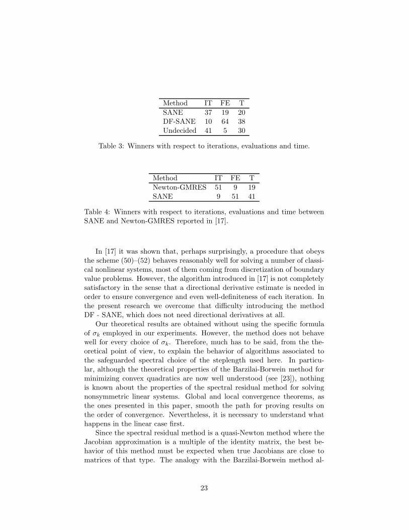
Method IT FE TSANE 37 19 20DF-SANE 10 64 38Undecided 41 5 30

Table 3: Winners with respect to iterations, evaluations and time.

Method IT FE TNewton-GMRES 51 9 19SANE 9 51 41

Table 4: Winners with respect to iterations, evaluations and time betweenSANE and Newton-GMRES reported in [17].

In [17] it was shown that, perhaps surprisingly, a procedure that obeysthe scheme (50)–(52) behaves reasonably well for solving a number of classi-cal nonlinear systems, most of them coming from discretization of boundaryvalue problems. However, the algorithm introduced in [17] is not completelysatisfactory in the sense that a directional derivative estimate is needed inorder to ensure convergence and even well-definiteness of each iteration. Inthe present research we overcome that difficulty introducing the methodDF - SANE, which does not need directional derivatives at all.

Our theoretical results are obtained without using the specific formulaof σk employed in our experiments. However, the method does not behavewell for every choice of σk. Therefore, much has to be said, from the the-oretical point of view, to explain the behavior of algorithms associated tothe safeguarded spectral choice of the steplength used here. In particu-lar, although the theoretical properties of the Barzilai-Borwein method forminimizing convex quadratics are now well understood (see [23]), nothingis known about the properties of the spectral residual method for solvingnonsymmetric linear systems. Global and local convergence theorems, asthe ones presented in this paper, smooth the path for proving results onthe order of convergence. Nevertheless, it is necessary to understand whathappens in the linear case first.

Since the spectral residual method is a quasi-Newton method where theJacobian approximation is a multiple of the identity matrix, the best be-havior of this method must be expected when true Jacobians are close tomatrices of that type. The analogy with the Barzilai-Borwein method al-

23

lows one to conjecture in which (more general) situations the method shouldbehave well. If the Jacobians are close to symmetric matrices with clusteredeigenvalues (see [21]) a good behavior of the Barzilai-Borwein method canbe predicted and, so, we also predict a fine behavior of the spectral resid-ual method. Very likely, in many practical situations the performance ofthe method should be improved using some kind of preconditioning thattransforms the Jacobian on a matrix with a small number of clusters ofeigenvalues. So, with respect to preconditioning features, the situation isanalogous to the one of Krylov-subspace methods. Preconditioned spectralgradient method for minimization were introduced in [19].

Our first set of experiments are discretization of boundary value prob-lems. In general, the Jacobians are positive definite, so that the mappingsF are generally monotone, or even strictly monotone. According to thecorollaries of Theorem 1 this favors the behavior of DF-SANE, but also fa-vors the behavior of almost every nonlinear-system solver. Since we are notusing preconditioning at all, in general eigenvalues are not clustered. Insome problems the Jacobians are well conditioned and in some other prob-lems they are not. Moreover, in some problems the Jacobian is singularat the solution. In principle ill-conditioning affects adversely both spectralmethods as Krylov subspace methods.

The second set of 22 problems does not show special characteristics fromthe point of view of positive definiteness or conditioning. Moreover, someof these problems have many solutions. In principle, we do not have strongreasons to predict a good behavior of DF-SANE, therefore the rather robustand efficient performance of the new algorithm for solving these problems isa pleasantly surprising fact that needs theoretical explanation.

We would like to finish pointing out that a different modification ofSANE, which uses watchdog techniques and coordinate search has been re-cently proposed in [14].

AcknowledgmentsWe are grateful to Raul Vignau, for his careful reading of the first draft

of this paper. We are also indebted to two anonymous referees for manysuggestions which greatly improved the quality and presentation of this pa-per.

References

[1] J. Barzilai and J. M. Borwein (1988). Two-point step size gradientmethods, IMA Journal of Numerical Analysis, 8, 141-148.

24

[2] S. Bellavia and B. Morini (2001). A globally convergent Newton-GMRES subspace method for systems of nonlinear equations, SIAMJournal on Scientific Computing, 23, 940–960.

[3] E. G. Birgin, J. M. Martınez and M. Raydan (2000). Nonmonotonespectral projected gradient methods on convex sets, SIAM Journalon Optimization, 10, 1196–1211.

[4] E. G. Birgin, J. M. Martınez and M. Raydan (2001). Algorithm 813:SPG - Software for convex-constrained optimization, ACM Transac-tions on Mathematical Software, 27, 340–349.

[5] E. G. Birgin, J. M. Martınez and M. Raydan (2003). Inexact spectralprojected gradient methods on convex sets, IMA Journal of Numer-ical Analysis, 23, 539–559.

[6] P. N. Brown and Y. Saad (1990). Hybrid Krylov methods for non-linear systems of equations, SIAM Journal on Scientific Computing,11, 450–481.

[7] P. N. Brown and Y. Saad (1994). Convergence theory of nonlinearNewton-Krylov algorithms, SIAM Journal on Optimization, 4, 297–330.

[8] Y. H. Dai and L. Z. Liao (2002). R-linear convergence of the Barzilaiand Borwein gradient method, IMA Journal of Numerical Analysis ,22, pp. 1–10.

[9] J. E. Dennis and R. B. Schnabel (1983), Numerical Methods forUnconstrained Optimization and Nonlinear Equations, Prentice-Hall,Englewood Cliffs, New Jersey.

[10] R. Fletcher (1990). Low storage methods for unconstrained optimiza-tion, Lectures in Applied Mathematics (AMS), 26, pp. 165–179.

[11] R. Fletcher (2001). On the Barzilai-Borwein method, Department ofMathematics, University of Dundee NA/207, Dundee, Scotland.

[12] M. Gasparo (2000). A nonmonotone hybrid method for nonlinearsystems, Optimization Methods and Software, 13, 79–94.

[13] L. Grippo, F. Lampariello and S. Lucidi (1986). A nonmonotone linesearch technique for Newton’s method, SIAM Journal on NumericalAnalysis, 23, 707–716.

25

[14] L. Grippo and M. Sciandrone (2005). Nonmonotone Derivative FreeMethods for Nonlinear Equations, Technical Report 01-05, DIS, Uni-versita di Roma “La Sapienza”.

[15] C. T. Kelley (1995), Iterative Methods for Linear and NonlinearEquations, SIAM, Philadelphia.

[16] W. La Cruz, J. M. Martınez and M. Raydan (2004). Spec-tral residual method without gradient information for solvinglarge-scale nonlinear systems: Theory and experiments, Techni-cal Report RT-04-08, Dpto. de Computacion, UCV, available inwww.kuainasi.ciens.ucv.ve/ccct/mraydan pub.html.

[17] W. La Cruz and M. Raydan (2003). Nonmonotone Spectral Meth-ods for Large-Scale Nonlinear Systems, Optimization Methods andSoftware, 18, 583–599.

[18] D. H. Li and M. Fukushima (2000). A derivative-free line search andglobal convergence of Broyden-like method for nonlinear equations,Optimization Methods and Software, 13, 181–201.

[19] F. Luengo, M. Raydan, W. Glunt and T. L. Hayden (2002). Pre-conditioned Spectral Gradient Method, Numerical Algorithms, 30,241–258.

[20] J. M. Martınez (2000). Practical quasi-Newton methods for solvingnonlinear systems, Journal of Computational and Applied Mathemat-ics, 124, 97–122.

[21] B. Molina and M. Raydan (1996). Preconditioned Barzilai-Borweinmethod for the numerical solution of partial differential equations,Numerical Algorithms, 13, pp. 45–60.

[22] J. M. Ortega and W. C. Rheinboldt (1970). Iterative solution of non-linear equations in several variables, Academic Press, New York.

[23] M. Raydan (1993). On the Barzilai and Borwein choice of thesteplength for the gradient method, IMA Journal on Numerical Anal-ysis, 13, 321–326.

[24] M. Raydan (1997). The Barzilai and Borwein gradient method forthe large scale unconstrained minimization problem, SIAM Journalon Optimization, 7, 26–33.

26