Spectral induced polarization measurements for predicting ... fileization (SIP) phenomena are...

Hydrol. Earth Syst. Sci., 17, 4079–4094, 2013www.hydrol-earth-syst-sci.net/17/4079/2013/doi:10.5194/hess-17-4079-2013© Author(s) 2013. CC Attribution 3.0 License.

Hydrology and Earth System

SciencesO

pen Access

Spectral induced polarization measurements for predicting thehydraulic conductivity in sandy aquifers

M. Attwa 1,2 and T. Günther3

1Geology Department, Faculty of Science, Zagazig University, 44519 Zagazig, Egypt2Geophysical Engineering Department, Faculty of Engineering, Ankara University, 6200 Ankara, Turkey3Leibniz Institute for Applied Geophysics (LIAG), 30655 Hannover, Germany

Correspondence to:M. Attwa ([email protected])

Received: 22 February 2013 – Published in Hydrol. Earth Syst. Sci. Discuss.: 29 April 2013Revised: 5 August 2013 – Accepted: 5 September 2013 – Published: 22 October 2013

Abstract. Field and laboratory spectral induced polariza-tion (SIP) measurements are integrated to characterize thehydrogeological conditions at the Schillerslage test site inGermany. The phase images are capable of monitoring thinpeat layers within the sandy aquifers. However, the field re-sults show limitations of decreasing resolution with depth.In comparison with the field inversion results, the SIP lab-oratory measurements show a certain shift in SIP responsedue to different compaction and sorting of the samples. TheSIP data are analyzed to derive an empirical relationshipfor predicting the hydraulic conductivity (K). In particular,two significant but weak correlations between individual realresistivities (ρ′) and relaxation times (τ ), based on a De-bye decomposition (DD) model, with measuredK are foundfor the upper groundwater aquifer. The maximum relaxationtime (τmax) and logarithmically weighted average relaxationtime (τlw) show a better relation withK values than the me-dian valueτ50. A combined power law relation between in-dividual ρ′ and τ with K is developed with an expressionof A · (ρ′)B · (τlw)C , whereA, B andC are determined us-ing a least-squares fit between the measured and predictedK. The suggested approach with the calculated coefficientsof the first aquifer is applied for the second. Results showgood correlation with the measuredK indicating that the de-rived relationship is superior to single phase angle models asBörner or Slater models.

1 Introduction

A key prerequisite for reliable prediction of groundwatermovements is the hydraulic conductivity (K). The pumpingtest, grain size or coring sleeve analyses have traditionallybeen the standard methods used to evaluate the hydraulic pa-rameters of subsurface material for characterizing ground-water aquifers. These methods are expensive, slow and of-ten unavailable due to disturbance during drilling to get theborehole samples. Partly for these reasons, electrical meth-ods are playing an increasingly important role in predictingthe aquifer hydraulic’s parameters (e.g., Zisser et al., 2010a;and Khalil, 2012).

The relationship between direct current (DC) resistivityρ and K is first considered as this makes up the bulk ofthe pertinent literatures published over the last 30 yr (e.g.,Heigold et al., 1979; Niwas and Singhal, 1985). Further, therelation between the real conductivity part (σ ′) and perme-ability was discussed and numerically investigated by manyauthors (e.g., Sen et al., 1981; Huntley, 1986; Bernabe andRevil, 1995; and Frohlich et al., 1996). Empirical and semi-empirical relationships have been established in terms ofpower law relations between various aquifer parameters andthose obtained by resistivity measurements (e.g., Attwa etal., 2009). Because the hydraulic parameters depend on theporosity and the geometry of the pore space,K cannot beuniquely determined by DC resistivity alone without furtherassumptions (Hördt et al., 2007).

The induced polarization (IP) of non-metallic minerals isgenerally referred to as interface or membrane polarization(Marshall and Madden, 1959; Vinegar and Waxman, 1984).

Published by Copernicus Publications on behalf of the European Geosciences Union.

4080 M. Attwa and T. Günther: Spectral induced polarization measurements

In the absence of metallic conductors, spectral induced polar-ization (SIP) phenomena are commonly associated with po-larization effects related to an electrochemical double layer(EDL), which describes the organization of ionic chargesat the interface between solid and fluid (Revil and Florsch,2010). The EDL provides the conceptual background for theelectrochemical processes considered to be responsible fora large amount of the observed SIP response (e.g., Leroy etal., 2008; and Revil and Cosenza, 2010). Accordingly, bothohmic (i.e., amplitude) and capacitive (i.e., phase) parts ofinterface polarization contain additional information aboutthe textural characteristics of sedimentary rocks (e.g., Schön,1996; Kemna, 2000; Slater, 2007; and Blaschek and Hördt,2009).

By measuring chargeability or, equivalently, the phaseshift between current and voltage, information about the porespace can be gained. Previous workers have shown that the IPmechanisms can be very sensitive to changes in lithology andpore fluid chemistry (e.g., Pelton et al., 1978; Weller et al.,2010b; and Skold et al., 2011). Environmental examples forthe successful use of SIP include the detection of clay units(e.g., Hördt et al., 2009; Attwa et al., 2011; and Attwa andGünther, 2012), the detection of both organic and inorganiccontaminants (e.g., Olhoeft, 1984, 1985, 1992; Chen et al.,2008, 2012; and Abdel Aal et al., 2009, 2010) and hydraulicconductivity estimation (e.g., Tong and Tao, 2007). Althoughthe SIP method offers potential for subsurface structure andprocess characterization, in particular in hydrogeophysicaland biogeophysical studies (Kemna et al., 2012), it is not aswidely used as other electrical methods (e.g., DC resistivity),and its full potential has yet to be realized.

The hydrogeophysical research of the IP method hasshown that SIP data can be correlated with physical prop-erties of the pore space in non-metallic soils and rocks, suchas the specific surface area (Spor) andK (e.g., Pape et al.,1987; Börner et al., 1996; and Weller et al., 2010a). There isa growing interest in the use of SIP for a wide range of en-vironmental applications, in particular those focused on hy-drogeological investigations. A clear link between hydroge-ological properties and IP/SIP parameters has been empiri-cally documented by various studies (e.g., Binley et al., 2005;and Hördt et al., 2007). Binley et al. (2010), Kruschwitz etal. (2010) and Titov et al. (2010) also pointed out that the un-derstanding of the detailed nature and origin of such linkagesstill lies ahead.

Recently, new models have been developed to describethe complex conductivity of saturated and unsaturated sandsand clayey materials in the low frequency domain (Revil andFlorsch, 2010; Revil, 2012; Revil et al., 2012a, 2013a). Revilet al. (2013a) presented a comparison between recently de-rived petrophysical models and a new set of petrophysicalmeasurements including permeability, complex conductivity,and streaming potential data on saprolite core samples. Theyproved that the quadrature conductivity (i.e., polarization) isnot controlled by the diffuse layer (the outer component of

the electrical double layer) but more likely by the Stern layer(the inner layer of the electrical double layer). The surfaceconductivity is dominated by electromigration in the elec-trical diffuse layer coating the pore water–mineral interface.Revil (2013) indicated that the diffuse layer is not the maincontributor to low-frequency polarization of clayey materi-als and also that the Maxwell–Wagner polarization is notthe dominating mechanism of polarization at intermediatefrequencies. Accordingly, he presented an extremely simpleunified model based on the low-frequency polarization of theStern layer. This model is proposed for all sedimentary rocks,saturated and unsaturated clayey materials. It offers the pos-sibility to predict the conductivity and permittivity (or al-ternatively the quadrature conductivity) as a function of fre-quency, clay content, and clay mineralogy. It is also used topredict permeability in the critical frequency observed at lowfrequencies in the quadrature conductivity.

Laboratory SIP investigations covering a wide frequencyrange provide more information on the spectral behav-ior of conductivity amplitude and phase shift. There areno universal physically based models that describe thefrequency-dependent complex conductivity response of sed-iments and, consequently, macroscopic representations havebeen adopted in the literature (Binley et al., 2005). TheSIP response can be described as a superposition of relax-ation processes, which might reflect grain-size distribution(Lesmes and Morgan, 2001). The induced polarization de-cay contains much more information than single frequencyor total chargeability data that are often used in traditional IPmeasurements. Significant progress has been made over thelast decade in the understanding of the microscopic mecha-nisms of IP; however, integrated mechanistic models involv-ing different possible polarization processes at the grain/porescale are still lacking (Kemna et al., 2012).

Various conceptual and theoretical relaxation models ex-ist to describe the SIP mechanism within the rocks and therelaxation process after terminating the current. Different ap-proaches have been reported for the computation of the relax-ation time (τ ) distribution. One of the most popular models isdefined as Debye decomposition (DD) (Nordsiek and Weller,2008). The DD can be applied to any measured spectral datasets independently of whether the spectra exhibit constantphase, by the same performance as Cole–Cole or other be-havior (Weller et al., 2010b) present. Binley et al. (2005) usethe mean relaxation time (τm) from a Cole–Cole model ofthe complex resistivity to estimate the permeability of sand-stone. Their measurements reveal evidence of a relationshipbetweenτ and a dominant pore throat size.

Revil and Florsch (2010) presented a model indicatingthat the permeability depends linearly on relaxation time.Revil (2012) developed a new robust model named PO-LARIS describing the complex conductivity of shaly poorlysorted sand. He showed that the permeability can be pre-dicted inside 1 order of magnitude using the formation fac-tor F and the quadrature conductivity. Revil et al. (2013b)

Hydrol. Earth Syst. Sci., 17, 4079–4094, 2013 www.hydrol-earth-syst-sci.net/17/4079/2013/

M. Attwa and T. Günther: Spectral induced polarization measurements 4081

developed a simple polarization model accounting for the de-pendence of the in-phase and quadrature conductivities onthe porosity, cation exchange capacity (or specific surfacearea of the material), and salinity of the pore water for sim-ple supporting electrolytes like NaCl in isothermal condi-tions. They showed a linear relationship between the mainrelaxation time and the pore throat size for clean sand andclayey sand samples. Revil (2013) predicted the permeabilityfor various clean sands, clayey sands and sandstones using alow-frequency relaxation timeτ and the formation factorF .Accordingly, these studies indicate that there is a linear rela-tion between the relaxation time and the pore size character-istics and the permeability of the materials.

The main objective of this paper is to use the SIP fieldand laboratory data to predict theK of unconsolidated sandyaquifers at the hydrogeological test site Schillerslage, Ger-many. A practical empirical relation will be introduced to cal-culateK. The format of this paper is as follows: (a) SIP field(sounding and profiling) and laboratory data will be acquiredfor describing the geological and hydrogeological character-istics of the subsurface Quaternary aquifers. (b) Field andlaboratory SIP data are used to evaluate various publishedapproaches to predictK values. The Debye decompositionmodel (Nordsiek and Weller, 2008) is applied to determinetheτ from available laboratory SIP data. (c) The importanceof combining electrical resistivity (ρ′) andτ for computingK is emphasized. Finally, the calculatedK from field andlaboratory data using various approaches are compared withthose measured from the pumping test and coring sleeve in-formation.

2 Material and methods

The SIP technique is a complex multi-frequency extension ofthe DC resistivity. Alternating currents of various frequenciesare injected and the phase shift between voltage and currentsignals is measured in addition to the resistance (amplituderatio). If the porous medium consists of clay-free, uniformlysized particles, the IP decay curve would consist of a singleexponent decay of relaxation time constant,τ , (Vinegar andWaxman, 1984, 1987, 1988). Revil and Florsch (2010) as-sumed that the Cole–Cole time constant,τ , can be related tothe square of the grain diameterd as

τ =d2

8D, (1)

where D is the diffusion coefficient in the Stern layer,which is temperature dependent and varies∼ 2 % per degreeKelvin. Titov et al. (2010) showed the relationships betweenthe modal pore throat diameter (R) in µm and the charac-teristic mean relaxation time,τm in s. A positive logarithmicdependence was derived:

R = 16.8lnτm − 2.15; (2)

Titov et al. (2010) suggested that the polarization of the sand-stones is controlled with clay content. They also showed agood correlation betweenR and permeabilityk.

The estimated geoelectrical properties of earth materialsmay be represented by complex electrical resistivity (ρ∗):

ρ∗= ρ′

+ iρ′′, (3)

whereρ∗, ρ′ andρ′′ are the complex resistivity, real resistiv-ity part and the imaginary part ofρ∗, respectively, andϕ isthe phase angle ofρ∗ that can be also written as follows:

ϕ = arctan(ρ′′/ρ′). (4)

The relationship betweenK andσ ′ will depends on the phys-ical and chemical properties of mineral and pore fluids and itindicates whether electrolytic conductivity (σel) or interfacialconductivity (σint) dominates measuredσ ′. Traditionally, thereal part of resistivity (i.e., DC resistivity) has been used toestimateK values for unconsolidated aquifers. For exam-ple, positive or negative linear log–log relationships betweenK andρ′ andσ ′ have been explained by many authors (e.g.,Heigold et al., 1997; Purvance and Andricevic, 2000; Attwaet al., 2009; and Attwa, 2012), using

K = a(σ ′)b. (5)

To apply Eq. (5) it would be necessary to estimatea andb

based on the comparison of geoelectrical measurements withmeasuredK values (e.g., pumping tests or grain size analy-ses). For sandy clayey soils the correlation ofK with ρ′ isdirectly proportional on a large scale, but sometimes on a lo-cal scale the correlation is inversely proportional (Mazac etal., 1990; Attwa, 2012).

There exists a substantial volume of literatures demon-strating a power dependence of the imaginary part of con-ductivity (σ ′′) on Spor (e.g., Börner et al., 1996; Slater andLesmes, 2002; Slater et al., 2006; and Weller et al., 2010b).Börner et al. (1996) observed that the phase shift (ϕ) for mostof their samples was particularly constant over a broad fre-quency range and suggested an empirical relation to estimateK from data for one frequency only, preferably around 1 Hz.Consequently, the basic assumption of this model is that themeasured phase shift of complex conductivity is independentof measurement frequency. However, for most rocks, this as-sumption is not valid. The proposed model (PARIS equation,Pape et al., 1987) for a constant-phase-angle (CPA) to calcu-lateK (in m s−1) is

K =a

F(Spor)c, (6)

where a and c exponents are adjustable parameters,F isthe formation factor andSpor is the specific surface area.The parameters in Eq. (6), suggested by Pape et al. (1987),are valid for consolidated sedimentary rocks. Börner etal. (1996) modified Eq. (6) to be valid for unconsolidated

www.hydrol-earth-syst-sci.net/17/4079/2013/ Hydrol. Earth Syst. Sci., 17, 4079–4094, 2013


rocks. Whereas Pape et al. (1987) suggesteda = 0.00475for consolidated sediments, Börner et al. (1996) useda = 1instead. Here, we work witha = 0.00475, which was alsorecommended by Weller and Börner (1996) and Hördt etal. (2009) for unconsolidated sediments. The exponentc wasfound to be in the range 2.8 <c < 4.6 (Börner et al., 1996),depending on the method ofK measurements. Börner etal. (1996) presented a modification to Archie’s law to cal-culate theF as

F =σw

σ ′ − σ ′′/l, (7)

whereσw is the pore fluid conductivity. Börner et al. (1996)suggested to usel = 0.1 in unconsolidated sediments. Notethat Eqs. (6) and (7) are not universal, but they were appliedfor wide hydrogeological investigations (e.g., Börner et al.,1996; and Hördt et al., 2006, 2009).Spor was calculated afterWeller et al. (2010b) for unconsolidated sandy aquifers as

Spor = (σ ′′

0.0101)1/0.916, (8)

whereSpor is in µm−1 andσ ′′ in mS m−1.The second approach was suggested by Slater and

Lesmes (2002) using the CPA model. The Slater andLesmes (2002) model is based on a relationship of the imag-inary conductivity part with the diameter of the grain cor-responding to the smallest 10 percent portion of the sample(i.e.,d10). Furthermore, this approach is based on the inverserelation betweenK andσ ′′ around 1 Hz as

K =m

(σ ′′)n, (9)

whereσ ′′ is given in µS m−1. m andn are adjustable param-eters withm = (2.0± 0.3)10−4; n = 1.1± 0.2, andK is inm s−1. It is noticed that the exponent from Slater and Lesmesmodel (2002) is smaller than in the model of Börner etal. (1996); hereinafter these models are referred to as “Slatermodel” and “Börner model”, respectively.

It is generally accepted thatτ (tau) is controlled by thediffusion process (Revil and Cosenza, 2010) in the electro-chemical double layer (EDL). A power law relationship be-tween some relaxation time constants and permeability (k)

has been reported in published data sets (Binley et al., 2005;Kemna et al., 2005; Tong et al., 2006a, b; Koch et al., 2011):

k = aτ b, (10)

wherea andb are formation-specific parameters.Zisser et al. (2010b) established a power law relationship

between the mean relaxation time (τm) andSpor. They provedalso that the relationship between the median relaxation time(τ50) andSpor is stronger than that betweenτm andSpor. Ac-cordingly, in presence of a weak relation between theτ andthe permeability and/orK, this relation cannot be applied.

Weller et al. (2010a) presented a generalized power lawrelation using DC resistivity, chargeability (M), and meanrelaxation time (τm), which were derived from DD, to predictk for isotropic and anisotropic samples,

k = a · (ρ′)b · Mc· (τm)d . (11)

The four empirical parametersa, b, c andd are determinedby a multivariate regression analysis.

3 Geological overview and measurement strategy

The test site Schillerslage is located northeast of Hannoverand shows a typical geological structure for the Quaternarysediment basin of northern Germany. Based on borehole in-formation, two sandy aquifers separated by a fine-grained tilllayer can be recognized (Fig. 1, right). The upper aquifer,down to a depth of about 12 m, consists of medium to partlycoarse sand and thin interbedded peat layers. The aquicludetill layer with high clay content is, in general, 12 m to 16 mdeep and varies also in thickness. The lower aquifer (i.e.,the second one) of 5 m thickness consists of slightly limymedium grey sand and it is overlying Cretaceous marls.

The SIP measurements were started by measuring a sound-ing curve using a Schlumberger configuration with AB/2 val-ues from 1.5 to 125 m and MN/2 values of 0.5 and 5 m. Ad-ditionally, a short SIP profile (P1) was measured crossingthe borehole ENG_03 and the center of sounding curve (seeFig. 1). The IP profile P1 was measured using 21 electrodesand 2 m electrode spacing. The P1 profile was followed bymeasuring a long profile (P2) by using 36 remote units tocharacterize lateral heterogeneity. Moreover, electrode spac-ing of 7 m was used to acquire the 2-D data across the P2profile (Fig. 1, right).

SIP laboratory measurements were done on 33 core sam-ples at different depths (from 0.65 to 23.15 m) of wellsENG_03 and ENG_08 (close to ENG_03). Then, directK

measurements were carried out by Sass (2010) using cor-ing sleeves (16 samples) and grain size analysis (13 sam-ples), for the upper and lower aquifers, respectively. The cor-ing sleeves were carried out on whole cores (8 cm diame-ter and 100 cm length) and soil samples (6 cm diameter and4 cm length). For grain size analysis, we used equations af-ter Kozeny (1927) and Beyer (1964) to deriveK and foundthat the differences are insignificant. Both field and labora-tory SIP measurements were conducted to calculateK valuesusing various approaches. Nine laboratory SIP samples lo-cated at the same depth of those used for coring sleeves wereused to derive an empirical relationship for predictingK val-ues. The inverted field (sounding and profiling) and measuredlaboratory SIP data were correlated and evaluated to assessthe differences inK values.

The SIP measurements (resistivity amplitude and phaseangle) are conducted over a wide range of frequencies. Tominimize induction effects, a dipole–dipole configuration



1

2

3

4

5

6

7

Fig. 1. (left) Location map of Schillerslage test site (Germany), available borehole, SIP field 8

measurements and SIP profile numbers (inset map, © Google Earth map). (Right) Lithology of 9

the Schillerslage test site. 10

11

12

13

14

15

16

17

18

19

Fig. 1. (Left) Location map of the Schillerslage test site (Germany), available borehole, SIP field measurements and SIP profile numbers(inset map,©Google Earth map). (Right) Lithology of the Schillerslage test site.

was used to acquire the profile’s SIP data. The field and lab-oratory SIP measurements were carried out using SIP256Cand SIP Fuchs equipment, respectively, by Radic Research(Radic et al., 1998; Radic, 2004). The four-electrode de-vice SIP Fuchs measures the complex resistivity over almostseven decades of frequency (from 0.0457 to 12 kHz). On theother hand, the multi-electrode instrument SIP256C mea-sures the complex resistivity over more than three decades(from 0.625 to 1 kHz). In both instruments, the remote unitsregister the voltage or current measurements, digitize the dataand transfer them to controlling PC through a fiber optic ca-ble to avoid interference of the current supply cables withthe voltage measurement. Acquisition of very low-frequencydata is limited by the data acquisition time. For one profilethe total measuring time was about 2 h, which can easily be-come excessive if even lower frequencies (< 0.625 Hz) arerequired, even though the system efficiently measures volt-ages at all receiver channels simultaneously.

4 Inversion results and interpretation

A Gauss–Newton algorithm using a smoothness constraintwith fixed regularization was chosen for sounding and pro-filing inversions, which were done by using DC1dinv andDC2DInvRes softwares (Günther, 2004), respectively. The2-D inversion algorithm was implemented for a global reg-ularization scheme using a first-order smoothness constraint(Günther, 2004). As introduced by Constable et al. (1987),we used different weights for horizontal and vertical modelboundaries such thatax = λ andaz = λwz. The regulariza-tion parameter (λ) is a weight that adjusts the degree ofimportance of the model smoothness constraints versus thedata misfit. A small value ofλ (or wz) produces a highly

structured model with huge parameter contrasts, explainingdata well, whereas a big value will not be able to fit the databut provides a smooth model.

While the apparent resistivity/conductivity amplitudes arealmost constant over frequency, the phase shows inductive orcapacitive coupling at frequencies starting at about 10 Hz. Toavoid distortion by the coupling effect, only low frequencydata were used in the inversion process. The 2-D processingincluded the rejection of data points with bad quality from themeasured data, i.e., for which the stacking error was above1 %. In addition, 3 % error was added to the stacking error toaccount for systematic error components in absence of recip-rocal data.

4.1 Field inversion results and interpretation

Figure 2 shows the inversion results of the IP sounding at366 mHz. A good fit between the measured and theoreticalresistivity data can be observed (Fig. 2a). On the other hand,a bad comparison can be observed at AB/2 higher than 50 m(Fig. 2b, right). This can be attributed to the electromagneticcoupling, which can be noted by abrupt changes in the phaseangle readings.

The inversion results of resistivity amplitudes show a goodcomparison with the borehole data (Fig. 2c, left). A low-resistivity layer (< 50�m) can be noticed between the twoaquifers, corresponding to the till layer. At about 23 m depth,another low resistivity layer can be observed correspondingto the Cretaceous marl layer. These low resistivity layers arecharacterized by high phase angle values (Fig. 2d, left).

As in Olayinka and Weller (1997), the 1-D inversion re-sults and the borehole information were used as a startingmodel for 2-D inversion to constrain the inversion process.Figure 3 shows the inversion results of the profile P1. Low



20

21

22

23

24

25

26

Fig. 2. SIP sounding inversion results. Apparent resistivity amplitude (a) and phase angle (b) data 27

and the inversion results (c and d, respectively) in comparison with well ENG_03 (see Fig. 1). 28

29

30

31

32

33

34

35

36

37

38

Fig. 2. SIP sounding inversion results. Apparent resistivity amplitude(a) and phase angle(b) data and the inversion results(c and d,respectively) in comparison with well ENG_03 (see Fig. 1).

frequency (0.625 Hz) SIP data were used in the inversion pro-cess. For the 2-D inversion, the regularization anisotropy wasset towz = az/ax = 0.01 in order to achieve predominantlylayered structures. It is clear from the resistivity amplitude(Fig. 3a) that the resistivity decreases with depth. In compar-ison with the borehole data, the heterogeneities of thin layersare not well defined from the resistivity amplitude image;whereas within the upper sandy aquifer’s thin layers withhigh phases (> 8 mrad) and sharp boundaries they can be wellnoticed from the conductivity phase model (Fig. 3b), that cor-responds to the peat layers. At about 13 m depth, there is asharp boundary between low (< 4 mrad) and high phase val-ues (> 13 mrad) which corresponds to the boundary betweenthe second sandy aquifer and the till layer. The first sandyaquifer of low phase values coincidences with the boreholedata.

Figure 3c represents the coverage plot for the model ofprofile P1 (for location see Fig. 1). According to Gün-ther (2004), the zones of higher coverage values indicatethat the model can be reliably derived from the data. Conse-quently, the maximum depth of sensitive area is about 12 m(Fig. 3c) and beyond this depth the data will lose the capabil-ity to resolve the heterogeneity between sedimentary layers.Accordingly, the heterogeneity within the upper aquifer canbe well recognized (Fig. 3b).

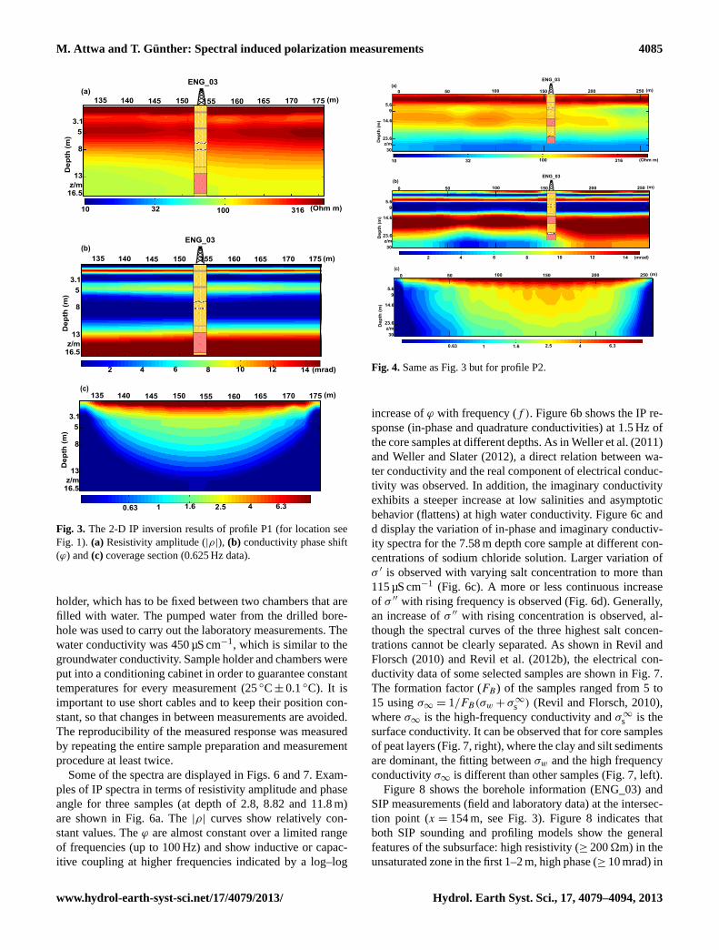
The inversion results of the other longer 2-D profile P2showed no great differences to P1. As with the P1 profile,we chose the 0.625 Hz data for presentation and further dis-cussion. The regularization parameter of z weight (wz) wasset toaz/ax = 0.01. The resistivity amplitude|ρ| image ex-hibits a predominantly layered structure with lateral varia-tions within these layers (Fig. 4a). The phase image of thecomplex electrical resistivity is shown in Fig. 4b. It exhibitsa clear layering in comparison with the resistivity amplitude

sections. Based on the coverage plot of the measured data,the maximum depth of the reliably inverted model is 30 m(Fig. 4c).

The high resistivity (> 300�m) complex of 5.6 m thick-ness (Fig. 4a) can be differentiated into three layers in thephase image (Fig. 4b); a low phase layer (< 4 mrad), whichcorresponds to sand, between two high phase (> 8 mrad) lay-ers corresponding to peats. Because of the high data coverageat 4.1 m depth (Fig. 4c), the peat layer can be well recog-nized in comparison with the inversion results of profile P1(Fig. 3b). The soil layer is followed by a medium resistivitylayer of∼ 18 m thickness, which can correspond to the sandyaquifer. This layer overlays a low resistivity layer (< 40�m)corresponding to Cretaceous marl. The heterogeneity withinthe sandy aquifers cannot be recognized. On the contrast, thephase shift image (Fig. 4b) represents the medium resistivitylayer in the form of two layers; the upper low phase layer(< 4 mrad) corresponding to the first sandy aquifer, which isfollowed by a high phase layer (> 13 mrad), corresponding tothe till layer. The lower sandy aquifer cannot be differentiatedfrom the upper till. This can be attributed to the presence ofa high phase layer (till) above the lower aquifer decreasingthe resolution with increasing depth and/or to the low datacoverage with increasing depth (Fig. 4c). At about 23.6 mdepth, this high phase layer is followed by the low phaselayer (< 7 mrad) corresponding to the Cretaceous marl. Thislayer cannot be recognized at the eastern part of the profile,which can be attributed to the bad data coverage (Fig. 4c).

4.2 Laboratory measurements and model comparison

In the laboratory, the samples were placed into a transpar-ent sample holder of the SIP Fuchs equipment (Fig. 5). Thesample has to be compacted and saturated in the sample



39

40

41

42

43

44

45

46

47

48

49

50

51

52

53

54

55

56

57

58

59

Fig. 3. The 2D IP inversion results of P1 profile (for location see Fig. 1). (a) The resistivity 60

amplitude (|ρ|), (b) conductivity phase shift ( ) and (c) coverage section (0.625 Hz data). 61

62

63

Fig. 3. The 2-D IP inversion results of profile P1 (for location seeFig. 1). (a) Resistivity amplitude (|ρ|), (b) conductivity phase shift(ϕ) and(c) coverage section (0.625 Hz data).

holder, which has to be fixed between two chambers that arefilled with water. The pumped water from the drilled bore-hole was used to carry out the laboratory measurements. Thewater conductivity was 450 µS cm−1, which is similar to thegroundwater conductivity. Sample holder and chambers wereput into a conditioning cabinet in order to guarantee constanttemperatures for every measurement (25◦C± 0.1◦C). It isimportant to use short cables and to keep their position con-stant, so that changes in between measurements are avoided.The reproducibility of the measured response was measuredby repeating the entire sample preparation and measurementprocedure at least twice.

Some of the spectra are displayed in Figs. 6 and 7. Exam-ples of IP spectra in terms of resistivity amplitude and phaseangle for three samples (at depth of 2.8, 8.82 and 11.8 m)are shown in Fig. 6a. The|ρ| curves show relatively con-stant values. Theϕ are almost constant over a limited rangeof frequencies (up to 100 Hz) and show inductive or capac-itive coupling at higher frequencies indicated by a log–log

64

65

66

67

68

69

70

71

72

73

74

75

76

77

78

Fig. 4. The 2D IP inversion results of P2 profile (for location see Fig. 1). (a) The resistivity 79

amplitude (|ρ|), (b) conductivity phase shift ( ) and (c) coverage section (0.625 Hz data). 80 81

82

83

84

85

86

87

Fig. 4.Same as Fig. 3 but for profile P2.

increase ofϕ with frequency (f ). Figure 6b shows the IP re-sponse (in-phase and quadrature conductivities) at 1.5 Hz ofthe core samples at different depths. As in Weller et al. (2011)and Weller and Slater (2012), a direct relation between wa-ter conductivity and the real component of electrical conduc-tivity was observed. In addition, the imaginary conductivityexhibits a steeper increase at low salinities and asymptoticbehavior (flattens) at high water conductivity. Figure 6c andd display the variation of in-phase and imaginary conductiv-ity spectra for the 7.58 m depth core sample at different con-centrations of sodium chloride solution. Larger variation ofσ ′ is observed with varying salt concentration to more than115 µS cm−1 (Fig. 6c). A more or less continuous increaseof σ ′′ with rising frequency is observed (Fig. 6d). Generally,an increase ofσ ′′ with rising concentration is observed, al-though the spectral curves of the three highest salt concen-trations cannot be clearly separated. As shown in Revil andFlorsch (2010) and Revil et al. (2012b), the electrical con-ductivity data of some selected samples are shown in Fig. 7.The formation factor (FB ) of the samples ranged from 5 to15 usingσ∞ = 1/FB(σw + σ∞

s ) (Revil and Florsch, 2010),whereσ∞ is the high-frequency conductivity andσ∞

s is thesurface conductivity. It can be observed that for core samplesof peat layers (Fig. 7, right), where the clay and silt sedimentsare dominant, the fitting betweenσw and the high frequencyconductivityσ∞ is different than other samples (Fig. 7, left).

Figure 8 shows the borehole information (ENG_03) andSIP measurements (field and laboratory data) at the intersec-tion point (x = 154 m, see Fig. 3). Figure 8 indicates thatboth SIP sounding and profiling models show the generalfeatures of the subsurface: high resistivity (≥ 200�m) in theunsaturated zone in the first 1–2 m, high phase (≥ 10 mrad) in



C1 C2P2P1

sample

water

88

89

90

91

92

93

94

95

96

97

98

99

Fig. 5. Layout of laboratory SIP measurements showing how the sample holder is measured 100

using the SIP Fuchs equipment. 101

102

103

104

105

106

107

108

109

110

111

Fig. 5.Layout of laboratory SIP measurements showing how the sample holder is measured using the SIP Fuchs equipment.

112

113

114

115

116

117

118

119

120

121

122

123 Fig. 6. (a) Exemplary SIP response at three samples at different depths (2.8 m, 8.82 m and 11.8 124

m) and (b) in-phase and quadrature conductivities (at 1.5 Hz) at different depths. (c and d) In-125

phase and quadrature conductivities at different water salinities of the collected sample at 7.58 m 126

depth. 127

128

129

130

131

132

133

134

135

Fig. 6. (a)Exemplary SIP response at three samples at different depths (2.8, 8.82 and 11.8 m) and(b) in-phase and quadrature conductivities(at 1.5 Hz) at different depths. (c, d) In-phase and quadrature conductivities at different water salinities of the collected sample at 7.58 mdepth.

till, marl and clay and low phases for the upper sandy aquifer(< 5 mrad). In the 2-D resistivity model, the resistivities ofthe upper aquifer and the till layer are in the same orderof amplitude. In spite of good correspondence of resistiv-ity amplitudes between IP 2-D inversion results and labora-tory data, the sounding curve inversion results show slightlylower resistivity values. In both models, thin peat layers ataround 2 m depth are detected by high phase values, whichcoincide with laboratory data. On the other hand, the 2-Dphase model shows the peat layer at 4.1 m with higher phase

values than the sounding model and laboratory data. Labo-ratory resistivity data show slightly lower values in the sec-ond aquifer than the sounding model and they are slightlyhigher than 2-D model. For the second aquifer, phase valuesfrom laboratory SIP are in general heterogeneous but oftenslightly higher than the sounding model and lower than the 2-D model. Clearly, a correspondence between the field phasemodels and laboratory data below till layer, i.e., the secondaquifer, cannot be observed.



Pore water conductivity (S/m)

0.00 0.05 0.10 0.15 0.20 0.25

0

1e-2

2e-2

3e-2

4e-2

5e-2

6e-2

Co

nd

ucti

vit

y (

S/m

)

Pore water conductivity (S/m)

0.00 0.05 0.10 0.15 0.20 0.25

4e-3

6e-3

8e-3

1e-2

1e-2

1e-2

2e-2

Co

nd

ucti

vit

y (

S/m

)

136

137

138

139

140

141

Fig. 7. High-frequency conductivity (σ ) versus pore water conductivity for core samples at 142

different depths. 143

144

145

146

147

148

149

150

151

152

153

154

155

156

Fig. 7.High-frequency conductivity (σ∞) versus pore water conductivity for core samples at different depths.

157

158

159

160

161

162

163

164

165 Fig. 8. Comparison of sounding, profiling and lab data at well ENG_03. Resistivity (left) and 166

phase (right). 167 168

169

170

171

172

173

174

175

176

177

178

179

180

181

182

183

Fig. 8.Comparison of sounding, profiling and lab data at well ENG_03. Resistivity (left) and phase (right).

5 Hydraulic conductivity ( K) estimation

To estimateK from IP results, three different approacheswere applied using Eqs. (5), (6) and (9). These approachesare meaningful in the saturated zone only (i.e., below 2 m).For calibration and the sake of clearness, the derivation ofK values was focused on the laboratory data for the upperaquifer. Then, theK will be predicted for the second aquiferbased on the derivedK of the upper aquifer. In order to ap-ply Eq. (5), a linear relationship should be achieved with agood correlation coefficient (R2) between the logarithms ofaquifer resistivityρ′ andK. We calculated the real part ofresistivity ρ′ using Eq. (4). Figure 9 shows log–log plot ofρ′ (at 1.5 Hz) against the measuredK using coring sleevesof the nine core samples (green solid circles). While there isa general trend of increasingρ′ with increasingK, the rela-tionship is weak (R2

= 0.4). Consequently, the estimation ofK from individualρ′ seems to be of limited applicability.

Both Börner and Slater models were applied to predictK

from the laboratory data and field inversion results in com-parison with the measuredKvalues. Note that the adjustableparameters for each model were derived from the correlationwith the measuredK values of the first aquifer and then they

were applied for the second aquifer. The inversion results ofIP field data (Fig. 8) at the intersection point (X = 154 m)were used to calculateK using both models. Equation (6)of Börner’s model was applied usingσw = 0.015 S m−1 andstandard values ofa = 0.00475 andl = 0.1, as explainedabove. The exponentc = 2.8 gave the best least-squares fitfor the measuredK values below the groundwater level.Spor was calculated using the Weller et al. (2010b) approach(Eq. 8). The second approach forK estimation after Slaterand Lesmes (2002) was applied usingm = 2.3× 10−4 andn = 0.9.

Figure 10 shows the applicability of both Börner and Slatermodels on the laboratory data in comparison with the mea-suredK values from coring sleeves and grain size analyses.The Börner approach represents bigger variations (∼ 10−7

to ∼ 10−2 m s−1), while the K estimation after the Slatermodel is varying in a smaller range (10−6 to 10−4 m s−1).Focusing on the sandy aquifers, it is clear that great differ-ences can be noticed between the results of both approachesfor the first aquifer. For the first aquifer, the calculatedK

values from Börner’s model are, in general, higher than themeasuredK values. On the contrast, a good correspondence



184

185

186

187

188

189

190

191

Fig. 9. Log-log plot of the measured resistivity versus the hydraulic conductivity (K) of nine core 192

samples from the 1st aquifer (see Fig. 1). Green solid circles (left) denote real resistivity parts 193

(ρʹ ), while the black circles (right) represent imaginary (σʹ ʹ ) conductivity parts. 194

195

196

197

198

199

200

201

202

203

204

205

206

207

Fig. 9. Log–log plot of the measured resistivity versusK of nine core samples from the first aquifer (see Fig. 1). Green solid circles (left)denote real resistivity parts (ρ′), while the black circles (right) represent imaginary (σ ′′) conductivity parts.

K (m/s)

1e-8 1e-7 1e-6 1e-5 1e-4 1e-3 1e-2 1e-1

dep

th (

m)

0

2

4

6

8

10

12

14

16

18

20

22

24

Own approach

Coring sleeves and

grain size analysis

Slater and Lesmes

model (2002)

Börner model (1996)

208

209

210

211

212

213

214

215

216

217

218

Fig. 10. Hydraulic conductivity of samples from borehole Eng_03. Black line: own approach. 219

Green line: from coring sleeves and grain size analysis using Kozeny equation. Pink line: from 220

Slater and Lesmes (2002) model. Blue line: from Börner et al. (1996) model. 221

222

223

224

225

226

227

228

229

230

Fig. 10.Hydraulic conductivity of samples from borehole Eng_03.Black line: own approach. Green line: from coring sleeves and grainsize analysis using Kozeny equation. Pink line: from the Slater andLesmes (2002) model. Blue line: from the Börner et al. (1996)model.

can be observed between the results of the two approaches inthe second aquifer. In general, the calculatedK values fromSlater’s model are lower than the measuredK values.

The calculatedK values from the field inverted data(sounding and profiling) show a wide range using bothBörner and Slater models. Figure 11 shows that the estima-tion of K values from sounding data is better than from 2-D data, in comparison with the measuredK values. TheKvalues from using the Börner model for the first aquifer ofsounding or profiling data are underestimated. On the otherhand, the estimatedK values from sounding data show agood correspondence with the measuredK for the secondaquifer (from 17 to 23 m depth) using the Börner model. Itis clear that the calculatedK values from sounding and pro-filing data for the till layer are smaller than the measuredK

values. Also, at 23 m depth the decreasingK values from

231

232

233

234

235

236

237

238

239

240

241

Fig. 11. Hydraulic conductivity at the location of borehole Eng_03. The green line: from coring 242

sleeves and grain size analysis using Kozeny equation. Red and pink lines: from Slater and 243

Lesmes (2002) model using sounding and profiling data, respectively. Brown and blue lines: 244

from Börner et al. (1996) model using 1D and 2D data, respectively. 245

246

247

248

249

250

251

252

253

Fig. 11.Hydraulic conductivity at the location of borehole Eng_03.The green line: from coring sleeves and grain size analysis us-ing Kozeny equation. Red and pink lines: from the Slater andLesmes (2002) model using sounding and profiling data, respec-tively. Brown and blue lines: from the Börner et al. (1996) modelusing 1-D and 2-D data, respectively.

both sounding and profiling data are likely to be caused bythe Cretaceous marl.

Based on the above results, it is clear that the use of val-ues from a CPA model, i.e., single frequency data as rep-resentative of the spectral response, is not valid to predictK. Consequently, the spectra were investigated using the DDto calculate the following parameters: DC resistivityρ′, to-tal chargeability (M) and different representative relaxationtimes (i.e., maximum relaxation timeτmax; median relaxationtime τ50 and logarithmically weighted average relaxation

time τlw

(τlw =

∑Mi ·logτ∑

Mi

)). Note that DD was applied after

removing the EM coupling effect fitting a double Cole–Colemodel (Pelton et al., 1978), i.e., one Cole–Cole term is asso-ciated to the coupling and another to the phase anomaly. Asin Weller et al. (2011), the DD successfully fitted the broad



254

255

256

257

258

259

260

261

262

263

264

265

266

267

268

269

270

271 Fig. 12. SIP lab data of one core sample at 6.68 m depth. (a) Resistivity amplitude (|ρ|). (b) 272

Measured phase (φ) (blue line) values, electromagnetic (EM) term (green line) and phase values 273

(red line) after removing EM effect. (c) The fitting between the phase values after removing EM 274

effect (blue line) and the fitted curve (red line). (d) The variation of spectral chargeability with 275

relaxation time by using DD model. 276

Fig. 12. SIP lab data of one core sample at 6.68 m depth.(a) Re-sistivity amplitude (|ρ|). (b) Measured phase (ϕ) (blue line) values,electromagnetic (EM) term (green line) and phase values (red line)after removing EM effect.(c) The fitting between the phase valuesafter removing EM effect (blue line) and the fitted curve (red line).(d) The variation of spectral chargeability with relaxation time byusing DD model.

shape range of complex conductivity spectra and was stablefor all samples and all salinities. Figure 12a shows an exam-ple of raw data (amplitude and phase) from a core sample at6.68 m depth. Figure 12b shows the correction of phase val-ues after electromagnetic removal. In addition, Fig. 12d re-flects a variation in spectral chargeability withτ by using DDfitting (Fig. 12c). For this sample, the minimum and max-imum values ofτ ′ are 10−4 s and 1 s, respectively, and thesmoothness factor (λ) used is 150. Phase data were quite ac-curate with stacking errors of about 0.1 mrad, which allowedthe spectral analysis of very small residual phases (Fig. 12).Due to the number of frequencies measured, the derived re-laxation time spectrum is relatively independent of statisticalerrors.

For our samples of the first aquifer, the relation ofτ (i.e.,τmax, τ50 andτlw) and the measuredK was studied. While

there is a general trend of increasingK with τ , the relation-ships are weak. Figure 13 shows an example of theτ–K re-lationship using different values ofτ . Although theτmax–K

and τlw–K relations show a better correlation thanτ50–K,the correlation coefficients are still low (R2

= 0.3 and 0.22,respectively). Correspondingly, the use of individualτ to pre-dict K using a power law relation will not be applicable.Moreover, the total of nine measuredK values is not enoughto apply the multivariate power law relation after Weller etal. (2010a).

5.1 A new approach

In general, the relaxation timeτ is the time required to estab-lish a stationary ionic distribution in the Stern layer coatinga grain of diameterd under the action of a static electricalfield (Revil and Florsch, 2010). The relation between the re-laxation time with the square of the grain size is representedin Eq. (1), which was confirmed by Titov et al. (2002) andLeroy et al. (2008).

The hydraulic and electrical conductivity of an aquifer de-pend on several factors; such as pore-size distribution, grainsize distribution and fluid salinity. If we consider theρ′

as a measure of grain size and pore-size distribution (e.g.,Kresnic, 2007; Chandra et al., 2008; Attwa et al., 2009; andAttwa, 2012), the aquifer resistivity could be well correlatedwith theK values of the aquifer (Eq. 5). Similarly, if we con-siderτ as a measure of the pore radius and pore size charac-teristics (Eqs. 1, 2), a link betweenτ andK can be consid-ered. The Debye decomposition of IP spectra yields a char-acteristic relaxation timeτ . These can be expressed in theform of Kα(ρ′)B(τ )C . Accordingly, theK can be calculatedusing

K = A(ρ′)B(τ )C, (12)

where theA coefficient and theB andC exponents are deter-mined by a regression analysis of the logarithmic quantitiesτ andK. This methodology was adopted for the estimationof the K when there is a general trend of increasing or de-creasing both individualρ′ andτ with K.

5.2 Correlation studies and testing methodology

In the cases ofρ′–K or τ–K relationships, the correlationsare weak but the there is a general increase ofρ′ andτ withthe measuredK values (Figs. 9 and 13, respectively). Equa-tion (13) was applied to the lab data collected from the upper(first) aquifer. Then, the coefficientsA and the exponents (B

andC) were used to predict theK values of the lower aquifer(i.e., the second one). Theρ′τ–K relation was studied usingτmax, τ50 (corresponds to the mean relaxation time as pro-posed by Zisser et al. (2010b) andτlw . A strong correlationcoefficient (R2

= 0.81) was achieved betweenρ′τlw and themeasuredK (Fig. 14) for nine samples of the first aquifer.A multivariate power law relationship (A(ρ′)B(τlw)C) was



1e-4 1e-3 1e-2

K (

m/s

)

max

50

lw

R2= 0.3

K= 9*10-4 ( )0.09max

R2= 0.17

K= 7*10-4 ( )0.0850

R2= 0.22

K= 1*10-3 ( )0.13lw

1e-4

1e-3

277

278

279

280

281

282

283

284

285

Fig. 13. Log-log plot of the maximum relaxation time ( max), median relaxation time ( 50) and 286

weighted average relaxation time ( lw) against the measured hydraulic conductivity (K) of nine 287

core samples from the 1st aquifer (see Fig. 1). 288

289

290

291

292

293

294

295

296

297

298

Fig. 13.Log–log plot of the maximum relaxation time (τmax), me-dian relaxation time (τ50) and weighted average relaxation time(τlw ) against the measuredK of nine core samples from the firstaquifer (see Fig. 1).

1e-2 1e-1 1e+0

1e-4

1e-3

K (

m/s

)

'

lw'50'

max'

R2= 0.45

K= 5*10-4 ( )0.13max'

R2= 0.6

K= 7*10-4 ( )0.4650'

R2= 0.81

K= 6*10-4 ( )0.73lw'

299

300

301

302

303

304

305

306

307

308

309

310

Fig. 14. Log-log plot of the maximum relaxation time ( max), median relaxation time ( 50) and 311

weighted average relaxation time ( lw) multiplied by ρʹ against the measured hydraulic 312

conductivity (K) of nine core samples from the 1st aquifer (see Fig. 1). 313

314

315

316

Fig. 14.Log–log plot ofτmax, τ50 andτlw multiplied byρ′ againstthe measuredK of nine core samples from the first aquifer (seeFig. 1).

examined and it was observed that the exponentsB andC

are nearly equal;K = 0.00012 (ρ′)1.08(τlw)0.8. However, dueto the limited number of data points we fixed them to beequal (i.e.,K = A(ρ′τ)B), thus decreasing the number of un-knowns.A andB were calculated for the upper aquifer andthey were 0.0006 and 0.73, respectively. Based on these re-sults, Eq. (13) was applied for the all core samples of bothaquifers using the deduced coefficientA and exponentB.Figure 10 shows the calculatedK values using Eq. (13)in comparison with the measuredK values and the calcu-latedK values from single frequency approaches. In com-parison with Eqs. (6) and (9), Eq. (13) shows the lowestmean-squared logarithmic error of fit (Tong and Tao, 2008),

ε2=

1

N

N∑i=1

[lnKm (i) − lnKc(i)]2 , δ = eε, (13)

whereN is the number of samples (in this paper it is 29),Km(i) and Kc(i) are the measured and computedK byconventional measurements and various approaches, respec-tively, andδ is the error factor. For Börner and Slater models,theδ values were 3.5 and 3.6, respectively. On the other hand,the δ was 1.4 for the proposed approach (Eq. 13). Accord-ingly, Eq. (13) is at least applicable at this test site (Fig. 10).

6 Discussion

Since it is hard to gain a full control of the subsurface struc-tures in natural geological environments during the 2-D in-version, the discrepancy between 1-D and 2-D inversion re-sults can be observed (Fig. 8). Because the 2-D inversionprocess is carried out using a fixed mesh size, the small IPresponse can be embedded within the general IP responseof the layer, which could be amplified during the inversionprocess. On the other hand, the 1-D inversion shows the IPresponse for a part of a layer with depth and accordingly, thelateral effect of IP response will be ignored.

Based on the inversion results of both sounding and pro-file P1, it is clear that the upper aquifer can be well defined,however we still have limitations in imaging the lower one.These limitations include an electromagnetic coupling withincreasing current electrode spacing of the sounding and thepenetration depth of the 2-D imaging. In general, our field in-version results indicate that the upper and lower boundariesof the upper (first) aquifer can be well defined from the phasevalues. The upper boundary of the lower sandy aquifer (i.e.,the second one) appears deeper than in the borehole, whichcan be attributed to the observed misfit between the raw andfitted phase angle data (Fig. 2, right). Also, there is a differ-ence of the phase behavior of the peat layer between the lab-oratory, sounding and profiling results (Fig. 8, right). Zanettiet al. (2011) and Ponziani et al. (2011) reported high phasevalues for buried tree root samples using laboratory exper-iments. They showed that a regular distribution of the poresize in diffuse porous woods leads to a stronger polarizationeffect.

As in Weller et al. (2006) and Revil et al. (2012b), a con-siderable variation in the spectra of conductivity amplitudeand phase shift can be observed in laboratory investigationsof peat, wood and soil samples. Weller et al. (2006) con-cluded that characteristic features of phase spectra can beused to detect wooden relics of trackways or pile dwellingfrom laboratory investigations. Revil et al. (2012b) devel-oped a quantitative model to investigate the frequency do-main induced polarization response of suspensions of bacte-ria and bacteria growth in porous media. They showed thatthe induced polarization of bacteria (α polarization) is re-lated to the properties of the electrical double layer of the



bacteria. The high IP effect can be attributed to the surface ofthe bacteria, which is highly charged due to the presence ofvarious structures extending away from the membrane intothe pore water solution. Consequently, the dead cells (i.e.,organic material) will show low IP effects.

The inspection of both sensitivity models and the inver-sion results of IP data is efficient in evaluating the reliabil-ity of the interpretation. The IP profiles (Figs. 3, 4) show ahigh polarization effect of the peat layer compared to labora-tory and sounding results. The coverage model demonstratesthat the reliable results concentrate up to a maximum depthof 16.5 m, which is only sufficient to cover the upper sandyaquifer. Because we have bad data coverage and electromag-netic coupling effects with increasing electrode spacing, thesecond aquifer cannot be imaged well. Accordingly, accu-rateK values of the lower aquifer from the IP field data can-not be expected. Figure 8 shows slight differences betweenfield data inversion results and laboratory data up to the tilllayer (∼ 13 m depth). Koch et al. (2011) stated that changesin compaction and sorting of samples cause a certain shiftin the SIP response but did not fundamentally alter the over-all picture. Accordingly, the modification of pore space andgrain size characteristics of original samples through com-paction of preparing the lab sample will change the SIP re-sponse, while the chemistry of the saturation pore fluid iskept constant.

Regarding the above results, the proposed IP–K relation-ships based on single frequency models appear inappropriatefor the unconsolidated heterogeneous sediments under inves-tigation. Clearly, there are limitations of using both Börnerand Slater models. In order to apply the single frequencymodels (Eqs. 6, 9) of both Börner et al. (1996) and Slater andLesmes (2002), certain conditions are required: (a) a constantphase angle over a wide frequency range, (b) a direct relationbetweenSpor andσ ′′ and (c) an inverse relation between themeasuredK andσ ′′. Figure 6 shows noticeable differences inphase angle with frequencies and it would appear inappropri-ate to use a single frequency complex measure as a represen-tative of IP spectra. The correlation betweenSpor andσ ′′ can-not be proved becauseSpor values were not measured (i.e., byBET measurements). Here, the correlation betweenSpor andσ ′′ cannot be proved becauseSpor values were not measured(i.e., by BET measurements). Because Eq. (8) after Weller etal. (2010b) was derived from an extensive sample database,the direct relation can be shown betweenSpor andσ ′′ for un-consolidated sediments. Moreover, Fig. 9 shows that the rela-tionship betweenσ ′′ andK is weak and not linear, althougha general decrease ofσ ′′ with K can be observed. The ex-istence of laboratory data over one decade could be the rea-son for this weak relation. Therefore, the models of Börnerand Slater seem to be of limited applicability at this test site.Compared with the overall lithology and measuredK values,the results from the Slater model appear more realistic thanthose from the Börner model, but, in general, the predictedK values are too small.

Since phase spectra of unconsolidated sediments typicallyshow frequency dependence, it is difficult to obtain a constantphase angle behavior over a limited frequency range for inho-mogeneous unconsolidated aquifers; multiple frequency dataare required to study the spectral behavior and to derive theK values. Our laboratory measurements of inhomogeneoussandy aquifers show a weak relationship between the mea-sured hydraulic conductivity and the maximum, median andweighted average relaxation time. Independently of the soiltexture, soil compaction has an influence on both the con-ductive properties (Seladji et al., 2010) and the polarizationresponse (Koch et al., 2011) of porous media. Accordingly,the weak correlation betweenK andτ can be attributed tothe compaction and sieving of the core samples from prepar-ing the laboratory measurements (Koch et al., 2011). Con-sequently, other physical parameters, which show a relationwith the measuredK, are required to support theK–τ re-lationship. Since the aquifer resistivities show a positive di-rect relation with the measuredK values, a multiplicationof τ and aquifer resistivities shows a good power law rela-tionship to estimate theK. In our study, the logarithmicallyweighted average relaxation time shows superior results ofpredicting theK compared with the mean relaxation timeused by Weller et al. (2010a) and the median relaxation timerecommended by Zisser et al. (2010b).

7 Conclusions

The goal of this study was to use SIP field and labora-tory measurements to characterize the hydrogeological con-ditions of the Schillerslage test site in Germany. The SIPmethod provided a tool for imaging subsurface hydrogeo-logical parameters of unconsolidated inhomogeneous sedi-ments. The improved Debye decomposition procedure wasused to calculate (τ ) values from the measured spectra. Wehave reached the following conclusions.

1. In our particular case, the IP inversion results indicatedthat the understanding of SIP signatures from labora-tory data can be achieved in field applications. Theresults here suggested that SIP is clearly able to dif-ferentiate lithological heterogeneities within unconsol-idated sediments.

2. The combination of field and laboratory IP measure-ments was recommended to evaluate the geologicalsituation and the accuracy of the interpretation (e.g.,changes in compaction and sorting of samples resultedin a certain shift in the SIP response between labora-tory and field inversion results). The mentioned recom-mendation provided a means to (i) overcome the spec-tral limitations resulting from EM coupling effects,which mask the SIP response at higher frequencies,and (ii) to examine the influence of physical and chem-ical properties of laboratory samples on SIP response.



3. Hydraulic conductivity estimates showed that singlefrequency models (Börner et al., 1996, and Slater andLesmes, 2002) used to predictK were inappropriateaccording to our investigations. However, the Slaterand Lesmes (2002) model yielded more realistic re-sults than the model of Börner et al. (1996). These canbe attributed to (i) the different type of sediments usedto derive the different approaches and (ii) because theassumption that the phase shift is constant over a widefrequency range was not achieved in our data. There-fore, the prediction ofK was examined using the re-laxation time (τ ). It was observed that a direct relationbetween theK andτ was not successful. In addition,the relation between the real resistivity part (ρ′) andK

was weak. Another practical application ofρ′τ–K wastested.

4. Our results revealed that the integration of the logarith-mic weighted average relaxation time (τlw) and DC re-sistivity yielded a power law relation to predict theK

of unconsolidated sandy aquifers particularly if onlyfew data points are present for correlation. However,it would be more meaningful if the above relation istested in areas with diverse geological environments.Moreover, with the number of samples increasing, amultivariate power law relation (K = A(ρ′)B(τlw)C)

is expected to improve the prediction ofK values and,consequently, this relation should be examined.

5. The present approach offers the possibility to use thefield data to monitor hydrogeological parameters us-ing the SIP components. A limited range of hydraulicconductivity variation over the study area can be ob-served and, consequently, the derived equation in thisstudy is not expected to apply to other areas but themethodology will.

6. Further work including lab measurements is requiredto study the spectral behavior of the peat layer. In ad-dition, application of recent universal models for cal-culating the specific surface area and the permeabilityusing the formation factors are desirable in compari-son with the approaches we used in this paper. Takingthese points into account can improve the accuracy ofpredicting the hydraulic conductivity measurements.In this framework a further use of the recent models(universal functions) can be suggested to account forthe dependence of the in-phase and quadrature con-ductivities on the porosity, cation exchange capacity(or specific surface area of the material), and salinity ofthe pore water for simple supporting electrolytes likeNaCl in isothermal conditions (Revil, 2013; Revil etal., 2013a, b).

Acknowledgements.We would like to thank Ahmet Basokur forhis careful review of the manuscript, which has improved thereadability of the text. A part of this paper has been presented at theinternational Workshop on Induced Polarization in Near-SurfaceGeophysics on 30 September/1 October 2009 in Bonn.

Edited by: T. P. A. Ferre

References

Abdel Aal, G. Z., Atekwana, E. A., Radzikowski, S., and Ross-bach, S.: Effect of bacterial adsorption on low frequency electri-cal properties of clean quartz sands and iron-oxide coated sands,Geophys. Res. Lett., 36, L04403, doi:10.1029/2008GL036196,2009.

Abdel Aal, G. Z., Atekwana, E. A., and Atekwana, E. A.: Effect ofbioclogging in porous media on complex conductivity signatures,J. Geophys. Res., 115, G00G07, doi:10.1029/2009JG001159,2010.

Attwa, M.: Field application “Data acquisition, processing and in-version”, in: Electrical methods “Practical guide for resistiv-ity imaging and hydrogeophysics”, edited by: Attwa, M., LAPLAMBERT Academic Publishing GmbH and Co. KG, 70–98,2012.

Attwa, M. and Günther, T.: Application of spectral induced po-larization (SIP) imaging for characterizing the near-surface ge-ology: an environmental case study at Schillerslage, Germany,Australian Journal of Applied Sciences, 6, 693–701, 2012.

Attwa, M., Günther, T., Grinat, M., and Binot, F.: Transimissivityestimation from sounding data of Holocene tidal flat depositsin the North Eastern part of Cuxhaven, Germany: Extended Ab-stracts: Near Surface 2009 – 15th European Meeting of Environ-mental and Engineering Geophysics, p. 029, 2009.

Attwa, M., Günther, T., Grinat, M., and Binot, F.: Evaluation of DC,FDEM and SIP resistivity methods for imaging a perched saltwa-ter and shallow channel within coastal tidal sediments, Germany,J. Appl. Geophys., 75, 656–670, 2011.

Bernabe, Y. and Revil, A.: Pore-scale heterogeneity, energy dissi-pation and the transport properties of rocks, Geophys. Res. Lett.,22, 1529–1532, 1995.

Beyer, W.: Zur Bestimmung der Wasserdruchlässigkeit vonKiesen und Sanden aus der Kornverteilung, Wasserwirtschaft –Wassertechnik (WWT), 6, 165–169, 1964.

Binley, A., Slater, L., Fukes, M., and Cassiani, G.: Relationshipbetween spectral induced polarization and hydraulic propertiesof saturated and unsaturated sandstone, Water Resour. Res., 41,W12417, doi:10.1029/2005WR004202, 2005.

Binley, A., Kruschwitz, S., Lesmes, D., and Kettridge, N.: Exploit-ing the temperature effects on low frequency electrical spectraof sandstone: a comparison of effective diffusion path lengths,Geophysics, 75, A43–A46, doi:10.1190/1.3483815, 2010.

Blaschek, R. and Hördt, A.: Numerical modeling of the IP effect atthe pore scale, Near Surf. Geophys., 7, 579–588, 2009.

Börner, F. D., Schopper, W., and Weller, A.: Evaluation of transportand storage properties in the soils and groundwater zone frominduced polarization measurements, Geophys. Prosp., 44, 583–601, doi:10.1111/j.1365-2478.1996.tb00167.x, 1996.

Chandra, S., Ahmed, S., Ram, A., and Dewandel, B.: Estimationof hard rock aquifer hydraulic conductivity from geoelectrical


http://dx.doi.org/10.1029/2008GL036196

http://dx.doi.org/10.1029/2009JG001159

http://dx.doi.org/10.1029/2005WR004202

http://dx.doi.org/10.1190/1.3483815

http://dx.doi.org/10.1111/j.1365-2478.1996.tb00167.x


measurements: A theoretical development with field application,J. Hydrol., 357, 281–227, doi:10.1016/j.jhydrol.2008.05.023,2008.

Chen, J., Kemna, A., and Hubbard, S. S.: A comparison betweenGauss-Newton and Markov-chain Monte Carlo-based methodsfor inverting spectral induced-polarization data for Cole-Cole pa-rameters, Geophysics, 73, F247–F259, 2008.

Chen, J., Hubbard, S. S., Williams, K. H., Flores Orozco, A., andKemna, A.: Estimating the spatiotemporal distribution of geo-chemical parameters associated with biostimulation using spec-tral induced polarization data and hierarchical Bayesian models,Water Resour. Res., 48, W05555, doi:10.1029/2011WR010992,2012.

Constable, S. C., Parker, R. L., and Constable, C. G.: Occam’s inver-sion: A practical algorithm for generating smooth models fromEM sounding data, Geophysics, 52, 289–300, 1987.

Frohlich, R. K., Fisher, J. J., and Summerly, E.: Electric-hydraulicconductivity correlation in fractured crystalline bedrock: CentralLandfill, Rhode Island, USA, J. Appl. Geophys., 35, 249–259,1996.

Günther, T.: Inversion methods and resolution analysis for the2D/3D reconstruction of resistivity structures from DC measure-ments, Ph.D. thesis, Univ. of Mining and Technology, Freiberg,Germany, 150 pp., 2004.

Heigold, P. C., Gilkeson, R. H., Cartwright, K., and Reed, P. C.:Aquifer transmissivity from surficial electrical methods, GroundWater, 17, 338–345, 1979.

Hördt, A., Blaschek, R., Kemna, A., and Zisser, N.: Hydraulic con-ductivity estimation from induced polarisation data at the fieldscale—the Krauthausen case history, J. Appl. Geophys., 62, 33–46, 2007.

Hördt, A., Druiventak, A., Blaschek, R., Binot, F., Kemna, A., Kr-eye, P., and Zisser, N.: Case histories of hydraulic conductivityestimation with induced polarization at the field scale, Near Surf.Geophys., 7, 529–545, 2009.

Huntley, D.: Relations between permeability and electrical resistiv-ity in granular aquifers, Ground Water, 24, 466–474, 1986.

Khalil, M. H.: Reconnaissance of freshwater conditions in a coastalaquifer: synthesis of 1D geoelectric resistivity inversion and hy-drogeological analysis, Near Surf. Geophys., 10, 427–441, 2012.

Kemna, A.: Tomographic inversion of complex resistivity – theoryand application, Ph.D. thesis, Ruhr Univ., Bochum, Germany,176 pp., 2000.

Kemna, A., Münch, H.-M., Titov, K., Zimmermann, E., andVereecken, H.: Relation of SIP relaxation time of sands to salin-ity, grain size and hydraulic conductivity: Extended Abstract:Near Surface 2005 – 11th European Meeting of Environmentaland Engineering Geophysics, p. 054, 2005.

Kemna, A., Binley, A., Cassiani, G., Niederleithinger, E., Revil, A.,Slater, L., Williams, K. H., Flores Orozco, A., Haegel, F.-H.,Hördt, A., Kruschwitz, S., Leroux, V., Titov, K., and Zimmer-mann, E.: An overview of spectral induced polarization methodfor near-surface applications, Near Surf. Geophys., 10, 453–468,doi:10.3997/1873-0604.2012027, 2012.

Koch, K., Kemna, A., Irving, J., and Holliger, K.: Impact ofchanges in grain size and pore space on the hydraulic conduc-tivity and spectral induced polarization response of sand, Hy-drol. Earth Syst. Sci., 15, 1785–1794, doi:10.5194/hess-15-1785-2011, 2011.

Kozeny, J.: Über kapillare Leitung des Wassers im Boden, Sitzungs-ber Akad Wiss Wien, 136, 271–306, 1927.

Kresnic, N.: Hydrogeology and Groundwater Modeling, 2nd Edn.,CRC Press, 2007.

Kruschwitz, S., Binley, A., Lesmes, D., and Elshenawy, A.: Texturalcontrols on low-frequency spectra of porous media, Geophysics,75, 113–123, doi:10.1190/1.3479835, 2010.

Lesmes, D. and Morgan, F. D.: Dielectric spectroscopy of sedimen-tary rocks, J. Geophys. Res., 106, 13329–13346, 2001.

Leroy, P., Revil, A., Kemna, A., Cosenza, P., and Ghor-bani, A.: Spectral induced polarization of water-saturatedpacks of glass beads, J. Colloid Interf. Sci., 321, 103–117,doi:10.1016/j.jcis.2007.12.031, 2008.

Marshall, D. J. and Madden, T. R.: Induced polarization, a study ofits causes, Geophysics, 24, 790–816, 1959.

Mazac, O., Cislerova, M., Kelly, W. E., Landa, I., and Venhodova,D.: Determination of hydraulic conductivities by surface geo-electrical methods, edited by: Ward, S. H., Geotechnical and en-vironmental geophysics, Society of Exploration Geophysicists,Tulsa, V2, 125–131, 1990.

Niwas, S. and Singhal, D. C.: Aquifer transimissivity of porous me-dia from resistivity data, J. Hydrol., 82, 143–153, 1985.

Nordsiek, S. and Weller, A.: A new approach to fitting induced-polarization spectra, Geophysics, 73, F235–F-245, 2008.

Olayinka, A. I. and Weller, A.: The inversion of geoelectrical datafor hydrogeological applications in crystalline basement areas ofNigeria, J. App. Geophys., 37, 103–115, 1997.

Olhoeft, G. R.: Clay-organic interactions measured with complexresistivity: Expanded Abstracts: Soc. Expl. Geophys 1984 – 54thAnnual International Meeting, 356–358, 1984.

Olhoeft, G. R.: Low-frequency electrical properties, Geophysics,50, 2492–2503, 1985.

Olhoeft, G. R.: Geophysical detection of hydrocarbon and organicchemical contamination, Proc. Symp. on the Application of Geo-physics to Engineering and Environmental Problems, 587–594,1992.

Pape, H., Riepe, L., and Schopper, J. R.: Theory of self-similarnetwork structures in sedimentary and igneous rocks and theirinvestigation with microscopical and physical methods, J. Mi-croscopy, 148, 121–147, 1987.

Pelton, W. H., Ward, S. H., Hallof, P. G., Sill, W. R., and Nelson, P.H.: Mineral discrimination and removal of electromagnetic cou-pling with multifrequency IP, Geophysics, 43, 588–609, 1978.

Ponziani, M., Ngan-Tillard, D. J. M., and Slob, E. C.: A new pro-totype cell to study electrical and geo-mechanical properties ofpeaty soils, Eng. Geol., 119, 74–81, 2011.

Purvance, D. and Andricevic, R.: Geoelectrical characterization ofthe hydraulic conductivity field and its spatial structure at vari-able scales, Water Resour. Res., 36, 2915–2924, 2000.

Radic, T.: Elimination of cable effects while multichannel SIP mea-surements: Extended Abstracts: Near Surface 2004 – 10th Eu-ropean Meeting of Environmental and Engineering Geophysics,2004.

Radic, T., Kretzschmar, D., and Niederleithinger, E.: Improvedcharacterization of unconsolidated sediments under field condi-tions based on complex resistivity measurements: Extended Ab-stracts: Near Surface 1998 – 4th European Meeting of Environ-mental and Engineering Geophysics, 1998.


http://dx.doi.org/10.1016/j.jhydrol.2008.05.023

http://dx.doi.org/10.1029/2011WR010992

http://dx.doi.org/10.3997/1873-0604.2012027

http://dx.doi.org/10.5194/hess-15-1785-2011

http://dx.doi.org/10.5194/hess-15-1785-2011

http://dx.doi.org/10.1190/1.3479835

http://dx.doi.org/10.1016/j.jcis.2007.12.031


Revil, A.: Spectral induced polarization of shaly sands: Influenceof the electrical double layer, Water Resour. Res., 48, W02517,doi:10.1029/2011WR011260, 2012.

Revil, A.: Effective conductivity and permittivity of unsaturatedporous materials in the frequency range 1 mHz–1 GHz, WaterResour. Res., 49, 306–327, doi:10.1029/2012WR012700, 2013.

Revil, A. and Cosenza, P.: Comment on “Generalized effective-medium theory of induced polarization” (M. Zhdanov, 2008,Geophysics, 73, F197–F211), Geophysics, 75, X7–X9, 2010.

Revil, A. and Florsch, N.: Determination of permeability from spec-tral induced polarization in granular media, Geophys. J. Int., 181,1480–1498, doi:10.1111/j.1365-246X.2010.04573.x, 2010.

Revil, A., Koch, K., and Holliger, K.: Is it the grain size or the char-acteristic pore size that controls the induced polarization relax-ation time of clean sands and sandstones?, Water Resour. Res.,48, W05602, doi:10.1029/2011WR011561, 2012a.

Revil, A., Atekwana, E., Zhang, C., Jardani, A., and Smith, S.: Anew model for the spectral induced polarization signature of bac-terial growth in porous media, Water Resour. Res., 48, W09545,doi:10.1029/2012WR011965, 2012b.

Revil, A., Skold, M., Hubbard, S. S., Wu, Y., Watson, D. B., andKaraoulis, M.: Petrophysical properties of saprolite from the OakRidge Integrated Field Research Challenge site, Tennessee, Geo-physics, 78, D21–D40, doi:10.1190/geo2012-0176.1, 2013a.

Revil, A., Eppehimer J. D., Skold, M., Karaoulis, M., GodinezL., and Prasad, M.: Low-frequency complex conductivity ofsandy and clayey materials, J. Colloid Interf. Sci., 398, 193–209,2013b.

Sass, S.: Applicability of geophysical measuring methods for de-termination ofK values in comparison to conventional measur-ing methods, Diploma thesis, Leibniz Univ., Hannover, Germany,2010.

Schön, J. H.: Physical properties of rocks-fundamental and princi-ples of petrophysics, Handbook of geophysical exploration, Seis-mic exploration, Pergamon Press, 583 pp., 1996.

Seladji, S., Cosenza, P., Tabbagh, A., Ranger, J., and Richard, G.:The effect of compaction on soil electrical resistivity: A labora-tory investigation, Eur. J. Soil Sci., 61, 1043–1055, 2010.

Sen, P. N., Scala, C., and Cohen, M. H.: A self-similar model forsedimentary rocks with application to the dielectric constant offused glass beads, Geophysics, 46, 781–795, 1981.

Skold, M., Revil, A., and Vaudelet, P.: The pH dependence of in-duced polarization of silica sands: Experiments and modeling,Geophys. Res. Lett., 38, L12304, doi:10.1029/2011GL047748,2011.

Slater, L.: Near surface electrical characterization of hydraulic con-ductivity: from petrophysical properties to aquifer geometries: areview, Surv. Geophys., 28, 169–197, 2007.

Slater, L. and Lesmes, D.: Electric-hydraulic relationships observedfor unconsolidated sediments, Water Resour. Res., 38, 1213,doi:10.1029/2001WR001075, 2002.

Slater, L., Ntarlagiannis, D., and Wishart, D.: On the relationshipbetween induced polarization and surface area in metal-sand andclay-sand mixtures, Geophysics, 71, A1–A5, 2006.

Titov, K., Komarov, V., Tarasov, V., and Levitski, A.: Theoreticaland experimental study of time-domain induced polarization inwater saturated sands, J. Appl. Geoph., 50, 417–433, 2002.

Titov, K., Tarasov, A., Ilyin, Y., Seleznev, N., and Boyd, A.: Rela-tionships between induced polarization relaxation time and hy-draulic properties of sandstone, Geophys. J. Int., 180, 1095–1106, 2010.

Tong, M. and Tao, H.: Experimental study of induced polarizationrelaxation time spectra of shaly sands, J. Petrol. Sci. Eng., 59,239–249, 2007.

Tong, M. and Tao, H.: Permeability estimation from complex resis-tivity measurement of shaly sand reservoir, Geophys. J. Int., 173,733–739, 2008.

Tong, M., Li., L., Wang, W., and Jiang, Y.: Determining capillary-pressure curve, pore size distribution and permeability from in-duced polarization of shaly sand, Geophysics, 71, N33–N40,2006a.

Tong, M., Li., L., Wang, W., and Jiang, Y.: A time-domain inducedpolarization method for estimating permeability in a shaly sandreservoir, Geophys. Prosp., 54, 623–631, 2006b.

Vinegar, H. J. and Waxman, M. H.: Induced polarization of shalysands, Geophysics, 49, 1267–1287, 1984.

Vinegar, H. J. and Waxman, M. H.: In-situ method for determiningpore size distribution, capillary pressure and permeability, USpatent, 4, 644, 283, 1987.

Vinegar, H. J. and Waxman, M. H.: In-situ method for determiningformation permeability, US patent, 4, 743, 854, 1988.

Weller, A. and Börner, F. D.: Measurements of spectral induced po-larization for environmental purposes, Environ. Geol., 27, 329–334, 1996.

Weller, A. and Slater, L.: Salinity dependence of complex con-ductivity of unconsolidated and consolidated materials: Com-parisons with electrical double layer models, Geophysics, 77,D185–D198, 2012.

Weller, A., Bauerochse, A., and Nordsiek, S.: Spectral induced po-larisation – a geophysical method for archaeological prospectionin peatlands, Journal of Wetland Archaeology, 6, 105–125, 2006.

Weller, A., Nordsiek, S., and Debschütz, W.: Estimation perme-ability of sandstone samples by nuclear magnetic resonanceand spectral-induced polarization, Geophysics, 75, E215–E226,2010a.

Weller, A., Slater, L., Nordsiek, S., and Ntarlagiannis, D.: On theestimation of specific surface per unit pore volume from inducedpolarization: A robust empirical relation fits multiple datasets,Geophysics, 75, WA105–WA112, 2010b.

Weller, A., Breede, K., Slater, L., and Nordsiek, S.: Effect of chang-ing water salinity on complex conductivity spectra, Geophysics,76, F315–F327, 2011.

Zanetti, C., Weller, A., Vennetier, M., and Mériaux, P.: Detection ofburied tree root samples by using geoelectrical, measurements: alaboratory experiment, Plant Soil, 339, 273–283, 2011.

Zisser, N., Kemna, A., and Nover, G.: Dependence of spectral in-duced polarization response of sandstone on temperature andits relevance to permeability estimation, J. Geophys. Res., 115,B09214, doi:10.1029/2010JB007526, 2010a.

Zisser, N., Kemna, A., and Nover, G.: Relationship betweenlow-frequency electrical properties and hydraulic permeabilityof low-permeability sandstones, Geophysics, 75, E131–E141,2010b.


http://dx.doi.org/10.1029/2011WR011260

http://dx.doi.org/10.1029/2012WR012700

http://dx.doi.org/10.1111/j.1365-246X.2010.04573.x

http://dx.doi.org/10.1029/2011WR011561

http://dx.doi.org/10.1029/2012WR011965

http://dx.doi.org/10.1190/geo2012-0176.1

http://dx.doi.org/10.1029/2011GL047748

http://dx.doi.org/10.1029/2001WR001075

http://dx.doi.org/10.1029/2010JB007526

Spectral induced polarization measurements for predicting ... fileization (SIP) phenomena are...

Documents

Transcript of Spectral induced polarization measurements for predicting ... fileization (SIP) phenomena are...