Spectral Algorithms for Data Analysis (draft)
123
Spectral Algorithms for Data Analysis (draft) Ravindran Kannan and Santosh S. Vempala September 27, 2021
Transcript of Spectral Algorithms for Data Analysis (draft)

Spectral Algorithms for Data Analysis
(draft)
Ravindran Kannan and Santosh S. Vempala
September 27, 2021

ii
Summary. Spectral methods refer to the use of eigenvalues, eigenvectors, sin-gular values and singular vectors. They are widely used in Engineering, Ap-plied Mathematics and Statistics. More recently, spectral methods have foundnumerous applications in Computer Science to “discrete” as well “continuous”problems. This book describes modern applications of spectral methods, andnovel algorithms for estimating spectral parameters.
In the first part of the book, we present applications of spectral methods toproblems from a variety of topics including combinatorial optimization, learningand clustering.
The second part of the book is motivated by efficiency considerations. A fea-ture of many modern applications is the massive amount of input data. Whilesophisticated algorithms for matrix computations have been developed over acentury, a more recent development is algorithms based on “sampling on thefly” from massive matrices. Good estimates of singular values and low rank ap-proximations of the whole matrix can be provably derived from a sample. Ourmain emphasis in the second part of the book is to present these sampling meth-ods with rigorous error bounds. We also present recent extensions of spectralmethods from matrices to tensors and their applications to some combinatorialoptimization problems.
Contents
I Applications 1
1 The Best-Fit Subspace 31.1 Singular Value Decomposition . . . . . . . . . . . . . . . . . . . . 31.2 Algorithms for computing the SVD . . . . . . . . . . . . . . . . . 71.3 The k-means clustering problem . . . . . . . . . . . . . . . . . . 81.4 Discussion . . . . . . . . . . . . . . . . . . . . . . . . . . . . . . . 11
2 Unraveling Mixtures Models 132.1 The challenge of high dimensionality . . . . . . . . . . . . . . . . 142.2 Classifying separable mixtures . . . . . . . . . . . . . . . . . . . . 15
2.2.1 Spectral projection . . . . . . . . . . . . . . . . . . . . . . 192.2.2 Weakly isotropic mixtures . . . . . . . . . . . . . . . . . . 202.2.3 Mixtures of general distributions . . . . . . . . . . . . . . 212.2.4 Spectral projection with samples . . . . . . . . . . . . . . 23
2.3 Learning mixtures of spherical distributions . . . . . . . . . . . . 242.4 An affine-invariant algorithm . . . . . . . . . . . . . . . . . . . . 29
2.4.1 Parallel Pancakes . . . . . . . . . . . . . . . . . . . . . . . 312.4.2 Analysis . . . . . . . . . . . . . . . . . . . . . . . . . . . . 32
2.5 Discussion . . . . . . . . . . . . . . . . . . . . . . . . . . . . . . . 33
3 Independent Component Analysis 353.1 Recovery with fourth moment assumptions . . . . . . . . . . . . 363.2 Fourier PCA and noisy ICA . . . . . . . . . . . . . . . . . . . . . 383.3 Discussion . . . . . . . . . . . . . . . . . . . . . . . . . . . . . . . 40
4 Recovering Planted Structures in Random Graphs 414.1 Planted cliques in random graphs . . . . . . . . . . . . . . . . . . 41
4.1.1 Cliques in random graphs . . . . . . . . . . . . . . . . . . 414.1.2 Planted clique . . . . . . . . . . . . . . . . . . . . . . . . 42
4.2 Full Independence and the Basic Spectral Algorithm . . . . . . . 444.2.1 Finding planted cliques . . . . . . . . . . . . . . . . . . . 45
4.3 Proof of the spectral norm bound . . . . . . . . . . . . . . . . . . 474.4 Planted partitions . . . . . . . . . . . . . . . . . . . . . . . . . . 504.5 Beyond full independence . . . . . . . . . . . . . . . . . . . . . . 51
iii

iv CONTENTS
4.5.1 Sums of matrix-valued random variables . . . . . . . . . . 534.5.2 Decoupling . . . . . . . . . . . . . . . . . . . . . . . . . . 554.5.3 Proof of the spectral bound with limited independence . . 56
4.6 Discussion . . . . . . . . . . . . . . . . . . . . . . . . . . . . . . . 59
5 Spectral Clustering 615.1 Project-and-Cluster . . . . . . . . . . . . . . . . . . . . . . . . . 61
5.1.1 Proper clusterings . . . . . . . . . . . . . . . . . . . . . . 625.1.2 Performance guarantee . . . . . . . . . . . . . . . . . . . . 625.1.3 Project-and-Cluster Assuming No Small Clusters . . . . . 64
5.2 Partition-and-Recurse . . . . . . . . . . . . . . . . . . . . . . . . 665.2.1 Approximate minimum conductance cut . . . . . . . . . . 665.2.2 Two criteria to measure the quality of a clustering . . . . 705.2.3 Approximation Algorithms . . . . . . . . . . . . . . . . . 715.2.4 Worst-case guarantees for spectral clustering . . . . . . . 75
5.3 Discussion . . . . . . . . . . . . . . . . . . . . . . . . . . . . . . . 76
6 Combinatorial Optimization via Low-Rank Approximation 79
II Algorithms 81
7 Power Iteration 83
8 Cut decompositions 858.1 Existence of small cut decompositions . . . . . . . . . . . . . . . 868.2 Cut decomposition algorithm . . . . . . . . . . . . . . . . . . . . 878.3 A constant-time algorithm . . . . . . . . . . . . . . . . . . . . . . 908.4 Cut decompositions for tensors . . . . . . . . . . . . . . . . . . . 918.5 A weak regularity lemma . . . . . . . . . . . . . . . . . . . . . . 928.6 Discussion . . . . . . . . . . . . . . . . . . . . . . . . . . . . . . . 93
9 Matrix approximation by Random Sampling 959.1 Matrix-vector product . . . . . . . . . . . . . . . . . . . . . . . . 959.2 Matrix Multiplication . . . . . . . . . . . . . . . . . . . . . . . . 969.3 Low-rank approximation . . . . . . . . . . . . . . . . . . . . . . . 97
9.3.1 A sharper existence theorem . . . . . . . . . . . . . . . . 1029.4 Invariant subspaces . . . . . . . . . . . . . . . . . . . . . . . . . . 1029.5 SVD by sampling rows and columns . . . . . . . . . . . . . . . . 1089.6 CUR: An interpolative low-rank approximation . . . . . . . . . . 1119.7 Discussion . . . . . . . . . . . . . . . . . . . . . . . . . . . . . . . 114

Part I
Applications
1


Chapter 1
The Best-Fit Subspace
To provide an in-depth and relatively quick introduction to SVD and its ap-plicability, in this opening chapter, we consider the best-fit subspace problem.Finding the best-fit line for a set of data points is a classical problem. A naturalmeasure of the quality of a line is the least squares measure, the sum of squared(perpendicular) distances of the points to the line. A more general problem, fora set of data points in Rn, is finding the best-fit k-dimensional subspace. SVDcan be used to find a subspace that minimizes the sum of squared distancesto the given set of points in polynomial time. In contrast, for other measuressuch as the sum of distances or the maximum distance, no polynomial-timealgorithms are known.
A clustering problem widely studied in theoretical computer science is thek-means problem. The goal is to find a set of k points that minimize the sum oftheir squared distances of the data points to their nearest facilities. A naturalrelaxation of the k-means problem is to find the k-dimensional subspace forwhich the sum of the distances of the data points to the subspace is minimized(we will see that this is a relaxation). We will apply SVD to solve this relaxedproblem and use the solution to approximately solve the original problem.
1.1 Singular Value Decomposition
For an n×n matrix A, an eigenvalue λ and corresponding eigenvector v satisfythe equation
Av = λv.
In general, i.e., if the matrix has nonzero determinant, it will have n nonzeroeigenvalues (not necessarily distinct). For an introduction to the theory ofeigenvalues and eigenvectors, several textbooks are available.
Here we deal with an m×n rectangular matrix A, where the m rows denotedA(1), A(2), . . . A(m) are points in Rn; A(i) will be a row vector.
If m 6= n, the notion of an eigenvalue or eigenvector does not make sense,since the vectors Av and λv have different dimensions. Instead, a singular value
3

4 CHAPTER 1. THE BEST-FIT SUBSPACE
σ and corresponding singular vectors u ∈ Rm, v ∈ Rn simultaneously satisfythe following two equations
1. Av = σu
2. uTA = σvT .
We can assume, without loss of generality, that u and v are unit vectors. Tosee this, note that a pair of singular vectors u and v must have equal length,since uTAv = σ‖u‖2 = σ‖v‖2. If this length is not 1, we can rescale both bythe same factor without violating the above equations.
Now we turn our attention to the value max‖v‖=1 ‖Av‖2. Since the rows ofA form a set of m vectors in Rn, the vector Av is a list of the projections ofthese vectors onto the line spanned by v, and ‖Av‖2 is simply the sum of thesquares of those projections.
Instead of choosing v to maximize ‖Av‖2, the Pythagorean theorem allowsus to equivalently choose v to minimize the sum of the squared distances of thepoints to the line through v. In this sense, v defines the line through the originthat best fits the points.
To argue this more formally, Let d(A(i), v) denote the distance of the pointA(i) to the line through v. Alternatively, we can write
d(A(i), v) = ‖A(i) − (A(i)v)vT ‖.
For a unit vector v, the Pythagorean theorem tells us that
‖A(i)‖2 = ‖(A(i)v)vT ‖2 + d(A(i), v)2.
Thus we get the following proposition. Note that ‖A‖2F =∑i,j A
2ij refers to the
squared Frobenius norm of A.
Proposition 1.1.
max‖v‖=1
‖Av‖2 = ||A||2F− min‖v‖=1
‖A−(Av)vT ‖2F = ||A||2F− min‖v‖=1
∑i
‖A(i)−(A(i)v)vT ‖2
Proof. We simply use the identity:
‖Av‖2 =∑i
‖(A(i)v)vT ‖2 =∑i
‖A(i)‖2 −∑i
‖A(i) − (A(i)v)vT ‖2
The proposition says that the v which maximizes ‖Av‖2 is the “best-fit”vector which also minimizes
∑i d(A(i), v)2.
Next, we claim that v is in fact a singular vector.
Proposition 1.2. The vector v1 = arg max‖v‖=1 ‖Av‖2 is a singular vector,and moreover ‖Av1‖ is the largest (or “top”) singular value.

1.1. SINGULAR VALUE DECOMPOSITION 5
Proof. For any singular vector v,
(ATA)v = σATu = σ2v.
Thus, v is an eigenvector of ATA with corresponding eigenvalue σ2. Conversely,an eigenvector of ATA is also a singular vector of A. To see this, let v be aneigenvector of ATA with corresponding eigenvalue λ. Note that λ is positive,since
‖Av‖2 = vTATAv = λvT v = λ‖v‖2
and thus
λ =‖Av‖2‖v‖2 .
Now if we let σ =√λ and u = Av/σ, it is easy to verify that u,v, and σ
satisfy the singular value requirements. The right singular vectors vi are thuseigenvectors of ATA.
Now we can also write
‖Av‖2 = vT (ATA)v.
Viewing this as a function of v, f(v) = vT (ATA)v, its gradient is
∇f(v) = 2(ATA)v.
Thus, any local maximum of this function on the unit sphere must satisfy
∇f(v) = λv
for some λ, i.e., ATAv = λv for some scalar λ. So any local maximum is aneigenvector of ATA. Since v1 is a global maximum of f , it must also be a localmaximum and therefore an eigenvector of ATA.
More generally, we consider a k-dimensional subspace that best fits the data.It turns out that this space is specified by the top k singular vectors, as statedprecisely in the following proposition.
Theorem 1.3. Define the k-dimensional subspace Vk as the span of the follow-ing k vectors:
v1 = arg max‖v‖=1
‖Av‖
v2 = arg max‖v‖=1,v·v1=0
‖Av‖
...
vk = arg max‖v‖=1,v·vi=0 ∀i<k
‖Av‖,

6 CHAPTER 1. THE BEST-FIT SUBSPACE
where ties for any arg max are broken arbitrarily. Then Vk is optimal in thesense that
Vk = arg mindim(V )=k
∑i
d(A(i), V )2.
Further, v1, v2, ..., vn are all singular vectors, with corresponding singular valuesσ1, σ2, ..., σn and
σ1 = ‖Av1‖ ≥ σ2 = ‖Av2‖ ≥ ... ≥ σn = ‖Avn‖.
Finally, A =∑ni=1 σiuiv
Ti .
Such a decomposition where,
1. The sequence of σi’s is nonincreasing
2. The sets ui, vi are orthonormal
is called the Singular Value Decomposition (SVD) of A.
Proof. We first prove that Vk are optimal by induction on k. The case k = 1 isby definition. Assume that Vk−1 is optimal.
Suppose V ′k is an optimal subspace of dimension k. Then we can choose anorthonormal basis for V ′k, say w1, w2, . . . wk, such that wk is orthogonal to Vk−1.By the definition of V ′k, we have that
||Aw1||2 + ||Aw22||+ . . . ||Awk||2
is maximized (among all sets of k orthonormal vectors.) If we replace wi by vifor i = 1, 2, . . . , k − 1, we have
‖Aw1‖2 + ‖Aw22‖+ . . . ‖Awk‖2 ≤ ‖Av1‖2 + . . .+ ‖Avk−1‖2 + ‖Awk‖2.
Therefore we can assume that V ′k is the span of Vk−1 and wk. It then followsthat ‖Awk‖2 maximizes ‖Ax‖2 over all unit vectors x orthogonal to Vk−1.
Proposition 1.2 can be extended to show that v1, v2, ..., vn are all singularvectors. The assertion that σ1 ≥ σ2 ≥ .... ≥ σn ≥ 0 follows from the definitionof the vi’s.
We can verify that the decomposition
A =
n∑i=1
σiuivTi
is accurate. This is because the vectors v1, v2, ..., vn form an orthonormal basisfor Rn, and the action of A on any vi is equivalent to the action of
∑ni=1 σiuiv
Ti
on vi.
Note that we could actually decompose A into the form∑ni=1 σiuiv
Ti by
picking vi to be any orthogonal basis of Rn, but the proposition actually
1.2. ALGORITHMS FOR COMPUTING THE SVD 7
states something stronger: that we can pick vi in such a way that ui is alsoan orthogonal set.
We state one more classical theorem. We have seen that the span of thetop k singular vectors is the best-fit k-dimensional subspace for the rows of A.Along the same lines, the partial decomposition of A obtained by using only thetop k singular vectors is the best rank-k matrix approximation to A.
Theorem 1.4. Among all rank k matrices D, the matrix Ak =∑ki=1 σiuiv
Ti is
the one which minimizes ‖A−D‖2F =∑i,j(Aij −Dij)
2. Further,
‖A−Ak‖2F =
n∑i=k+1
σ2i .
Proof. We have
‖A−D‖2F =
m∑i=1
‖A(i) −D(i)‖2.
Since D is of rank at most k, we can assume that all the D(i) are projections ofA(i) to some rank k subspace and therefore,
m∑i=1
‖A(i) −D(i)‖2 =
m∑i=1
‖A(i)‖2 − ‖D(i)‖2
= ‖A‖2F −m∑i=1
‖D(i)‖2.
Thus the subspace is exactly the SVD subspace given by the span of the first ksingular vectors of A.
1.2 Algorithms for computing the SVD
Computing the SVD is a major topic of numerical analysis [Str88, GvL96,Wil88]. Here we describe a basic algorithm called the power method.
Assume that A is symmetric.
1. Let x be a random unit vector.
2. Repeat:
x :=Ax
‖Ax‖
For a nonsymmetric matrix A, we can simply apply the power iteration to ATA.
Exercise 1.1. Show that with probability at least 1/4, the power iteration appliedk times to a symmetric matrix A finds a vector xk such that
‖Axk‖2 ≥(
1
4n
)1/k
σ21(A).

8 CHAPTER 1. THE BEST-FIT SUBSPACE
[Hint: First show that ‖Axk‖ ≥ (|x · v|)1/kσ1(A) where x is the starting vectorand v is the top eigenvector of A; then show that for a random unit vector x,the random variable |x.v| is large with some constant probability].
The second part of this book deals with faster, sampling-based algorithms.
1.3 The k-means clustering problem
This section contains a description of a clustering problem which is often calledk-means in the literature and can be solved approximately using SVD. Thisillustrates a typical use of SVD and has a provable bound.
We are given m points A = A(1), A(2), . . . A(m) in n-dimensional Eu-clidean space and a positive integer k. The problem is to find k points B =B(1), B(2), . . . , B(k) such that
fA(B) =
m∑i=1
(dist(A(i),B))2
is minimized. Here dist(A(i),B) is the Euclidean distance of A(i) to its nearestpoint in B. Thus, in this problem we wish to minimize the sum of squareddistances to the nearest “cluster center”. This is commonly called the k-meansor k-means clustering problem. It is NP-hard even for k = 2. A popular localsearch heuristic for this problem is often called the k-means algorithm.
We first observe that the solution is given by k clusters Sj , j = 1, 2, . . . k.The cluster center B(j) will be the centroid of the points in Sj , j = 1, 2, . . . , k.This is seen from the fact that for any set S = X(1), X(2), . . . , X(r) and anypoint B we have
r∑i=1
‖X(i) −B‖2 =
r∑i=1
‖X(i) − X‖2 + r‖B − X‖2, (1.1)
where X is the centroid (X(1) + X(2) + · · · + X(r))/r of S. The next exercisemakes this clear.
Exercise 1.2. Show that for a set of point X1, . . . , Xk ∈ Rn, the point Y thatminimizes
∑ki=1 |Xi−Y |2 is their centroid. Give an example when the centroid
is not the optimal choice if we minimize sum of distances rather than squareddistances.
The k-means clustering problem is thus the problem of partitioning a set ofpoints into clusters so that the sum of the squared distances to the means, i.e.,the variances of the clusters is minimized.
We define a relaxation of this problem that we may cal the ContinuousClustering Problem (CCP): find the subspace V of Rn of dimension at most kthat minimizes
gA(V ) =
m∑i=1
dist(A(i), V )2.

1.3. THE K-MEANS CLUSTERING PROBLEM 9
The reader will recognize that this can be solved using the SVD. It is easy tosee that the optimal value of the k-means clustering problem is an upper boundfor the optimal value of the CCP. Indeed for any set B of k points,
fA(B) ≥ gA(VB) (1.2)
where VB is the subspace generated by the points in B.
We now present a factor 2 approximation algorithm for the k-means cluster-ing problem using the relaxation to the best-fit subspace. The algorithm has twoparts. First we project to the k-dimensional SVD subspace, solving the CCP.Then we solve the problem in the low-dimensional space using a brute-forcealgorithm with the following guarantee.
Theorem 1.5. The k-means problem can be solved in O(mk2d/2) time when theinput A ⊆ Rd.
We describe the algorithm for the low-dimensional setting. Each set B of“cluster centers” defines a Voronoi diagram where cell Ci = X ∈ Rd : |X −B(i)| ≤ |X −B(j)| for j 6= i consists of those points whose closest point in B isB(i). Each cell is a polyhedron and the total number of faces in C1, C2, . . . , Ckis no more than
(k2
)since each face is the set of points equidistant from two
points of B.
We have seen in (1.1) that it is the partition of A that determines the bestB (via computation of centroids) and so we can move the boundary hyperplanesof the optimal Voronoi diagram, without any face passing through a point of A,so that each face contains at least d points of A.
Assume that the points of A are in general position and 0 /∈ A (a simpleperturbation argument deals with the general case). This means that each facenow contains d affinely independent points of A. We ignore the informationabout which side of each face to place these points and so we must try all pos-sibilities for each face. This leads to the following enumerative procedure forsolving the k-means clustering problem:

10 CHAPTER 1. THE BEST-FIT SUBSPACE
Algorithm: Voronoi-k-means
1. Enumerate all sets of t hyperplanes, such that k ≤ t ≤k(k − 1)/2 hyperplanes, and each hyperplane contains daffinely independent points of A. The number of sets is
at most(k2)∑t=k
((md
)t
)= O(mdk2/2).
2. Check that the arrangement defined by these hyperplanes
has exactly k cells.
3. Make one of 2td choices as to which cell to assign each
point of A which lies on a hyperplane
4. This defines a unique partition of A. Find the centroid
of each set in the partition and compute fA.
Now we are ready for the complete algorithm. As remarked previously, CCP canbe solved by Linear Algebra. Indeed, let V be a k-dimensional subspace of Rn
and A(1), A(2), . . . , A(m) be the orthogonal projections of A(1), A(2), . . . , A(m)
onto V . Let A be the m×n matrix with rows A(1), A(2), . . . , A(m). Thus A hasrank at most k and
‖A− A‖2F =
m∑i=1
|A(i) − A(i)|2 =
m∑i=1
(dist(A(i), V ))2.
Thus to solve CCP, all we have to do is find the first k vectors of the SVD ofA (since by Theorem (1.4), these minimize ‖A− A‖2F over all rank k matricesA) and take the space VSV D spanned by the first k singular vectors in the rowspace of A.
We now show that combining SVD with the above algorithm gives a 2-approximation to the k-means problem in arbitrary dimension. Let A = A(1), A(2), . . . , A(m)be the projection of A onto the subspace Vk. Let B = B(1), B(2), . . . , B(k) bethe optimal solution to k-means problem with input A.
Algorithm for the k-means clustering problem
• Compute Vk.
• Solve the k-means clustering problem with input A to obtain B.
• Output B.
It follows from (1.2) that the optimal value ZA of the k-means clustering problemsatisfies
ZA ≥m∑i=1
|A(i) − A(i)|2. (1.3)

1.4. DISCUSSION 11
Note also that if B = B(1), B(2), . . . , B(k) is an optimal solution to the k-means clustering problem and B consists of the projection of the points in Bonto V , then
ZA =
m∑i=1
dist(A(i), B)2 ≥m∑i=1
dist(A(i), B)2 ≥m∑i=1
dist(A(i), B)2.
Combining this with (1.3) we get
2ZA ≥m∑i=1
(|A(i) − A(i)|2 + dist(A(i), B)2)
=
m∑i=1
dist(A(i), B)2
= fA(B)
proving that we do indeed get a 2-approximation.
Theorem 1.6. The above algorithm for the k-means clustering problem finds afactor 2 approximation for m points in Rn in O(mn2 +mk3/2) time.
1.4 Discussion
In this chapter, we reviewed basic concepts in linear algebra from a geometricperspective. The k-means problem is a typical example of how SVD is used:project to the SVD subspace, then solve the original problem. In many ap-plication areas, the method known as “Principal Component Analysis” (PCA)uses the projection of a data matrix to the span of the largest singular vectors.There are several introducing the theory of eigenvalues and eigenvectors as wellas SVD/PCA, e.g., [GvL96, Str88, Bha97].
The application of SVD to the k-means clustering problem is from [DFK+04]and its hardness is from [ADHP09]. The following complexity questions areopen: (1) Given a matrix A, is it NP-hard to find a rank-k matrix D thatminimizes the error with respect to the L1 norm, i.e.,
∑i,j |Aij −Dij |? (more
generally for Lp norm for p 6= 2)? (2) Given a set of m points in Rn, is itNP-hard to find a subspace of dimension at most k that minimizes the sum ofdistances of the points to the subspace? It is known that finding a subspacethat minimizes the maximum distance is NP-hard [MT82]; see also [HPV02].

12 CHAPTER 1. THE BEST-FIT SUBSPACE
Chapter 2
Unraveling MixturesModels
An important class of data models are generative, i.e., they assume that data isgenerated according to a probability distribution D in Rn. One major scenariois when D is a mixture of some special distributions. These may be continuousor discrete. Prominent and well-studied instances of each are:
• D is a mixture of Gaussians.
• D is choosing the row vectors of the adjacency matrix of a random graphwith certain special properties.
For the second situation, we will see in Chapter 4 that spectral methods arequite useful. In this chapter, we study a classical generative model where theinput is a set of points in Rn drawn randomly from a mixture of probabilitydistributions. The sample points are unlabeled and the basic problem is tocorrectly classify them according the component distribution which generatedthem. The special case when the component distributions are Gaussians is aclassical problem and has been widely studied. In later chapters, we will revisitmixture models in other guises (e.g., random planted partitions).
Let F be a probability distribution in Rn with the property that it is aconvex combination of distributions of known type, i.e., we can decompose F as
F = w1F1 + w2F2 + · · ·+ wkFk
where each Fi is a probability distribution with mixing weight wi ≥ 0, and∑i wi = 1. A random point from F is drawn from distribution Fi with proba-
bility wi.Given a sample of points from F , we consider the following problems:
1. Classify the sample according to the component distributions.
2. Learn parameters of the component distributions (e.g., estimate theirmeans, covariances and mixing weights).
13

14 CHAPTER 2. UNRAVELING MIXTURES MODELS
The second problem is well-defined by the following theorem.
Theorem 2.1. A mixture of Gaussians can be uniquely determined by its prob-ability density function.
For most of this chapter, we deal with the classical setting: each Fi is aGaussian in Rn. In fact, we begin with the special case of spherical Gaussianswhose density functions (i) depend only on the distance of a point from the meanand (ii) can be written as the product of density functions on each coordinate.The density function of a spherical Gaussian in Rn is
p(x) =1
(√
2πσ)ne−‖x−µ‖
2/2σ2
where µ is its mean and σ is the standard deviation along any direction.
2.1 The challenge of high dimensionality
Intuitively, if the component distributions are far apart, so that a pair of pointsfrom the same component distribution are closer to each other than any pairfrom different components, then classification is straightforward. If the com-ponent distributions have a large overlap, then it is not possible to correctlyclassify all or most of the points, since points from the overlap could belong tomore than one component. To illustrate this, consider a mixture of two one-dimensional Gaussians with means µ1, µ2 and variances σ1, σ2. For the overlapof the distributions to be smaller than ε, we need the means to be separated as
|µ1 − µ2| ≥ C√
log(1/ε) maxσ1, σ2.
|µ1 − µ2| ≥ C√
log(1/ε) minσ1, σ2. If the distance were smaller than this bya constant factor, then the total variation (or L1) distance between the twodistributions would be less than 1 − ε and we could not correctly classify withhigh probability a 1−ε fraction of the mixture. On the other hand, if the meanswere separated as above, for a sufficiently large C, then at least 1 − ε of thesample can be correctly classified with high probability; if we replace
√log(1/ε)
with√
logm where m is the size of the sample, then with high probability, everypair of points from different components would be farther apart than any pairof points from the same component, and classification is easy. For example, wecan use the following distance-based classification algorithm (sometimes calledsingle linkage):
1. Sort all pairwise distances in increasing order.
2. Choose edges in this order till the edges chosen form exactly two connectedcomponents.
3. Declare points in each connected component to be from the same compo-nent distribution of the mixture.

2.2. CLASSIFYING SEPARABLE MIXTURES 15
Now consider a mixture of two spherical Gaussians, but in Rn. We claimthat the same separation as above with distance between the means measuredas Euclidean length, suffices to ensure that the components are probabilisticallyseparated. Indeed, this is easy to see by considering the projection of the mixtureto the line joining the two original means. The projection is a mixture of two one-dimensional Gaussians satisfying the required separation condition above. Willthe above classification algorithm work with this separation? The answer turnsout to be no. This is because in high dimension, the distances between pairs fromdifferent components, although higher in expectation compared to distancesfrom the same component, can deviate from their expectation by factors thatdepend both on the variance and the ambient dimension, and so, the separationrequired for such distance-based methods to work grows as a function of thedimension. We will discuss this difficulty and how to get around in more detailpresently.
The classification problem is inherently tied to the mixture being separable.However, the learning problem, in principle, does not require separable mixtures.In other words, one could formulate the problem of estimating the parametersof the mixture without assuming any separation between the components. Forthis learning problem with no separation, even for mixtures of Gaussians, thereis an exponential lower bound in k, the number of components, on the time andsample complexity. Most of this chapter is about polynomial algorithms for theclassification and learning problems under suitable assumptions.
2.2 Classifying separable mixtures
In order to correctly identify sample points, we require the overlap of distribu-tions to be small . How can we quantify the distance between distributions? Oneway, if we only have two distributions, is to take the total variation distance,
dTV (f1, f2) =1
2
∫Rn|f1(x)− f2(x)| dx,
where f1, f2 are density functions of the two distributions. The overlap of twodistributions is defined as 1 − dTV (f1, f2). We can require this to be large fortwo well-separated distributions, i.e., dTV (f1, f2) ≥ 1− ε, if we tolerate ε error.
This can be generalized in two ways to k > 2 components. First, we couldrequire the above condition holds for every pair of components, i.e., pairwiseprobabilistic separation. Or we could have the following single condition.
∫Rn
(2 max
iwifi(x)−
k∑i=1
wifi(x)
)+
dx ≥ 1− ε (2.1)
where
x+ =
x if x > 0
0 otherwise.

16 CHAPTER 2. UNRAVELING MIXTURES MODELS
The quantity inside the integral is simply the maximum wifi at x, minus thesum of the rest of the wifi’s. If the supports of the components are essentiallydisjoint, the integral will be 1.
For k > 2, it is not known how to efficiently classify mixtures when we aregiven one of these probabilistic separations. In what follows, we use strongerassumptions. Strengthening probabilistic separation to geometric separationturns out to be quite effective. We consider that next.
Geometric separation. For two distributions, we require ‖µ1−µ2‖ to belarge compared to maxσ1, σ2. Note this is a stronger assumption than that ofsmall overlap. In fact, two distributions can have the same mean, yet still havesmall overlap, e.g., two spherical Gaussians with different variances. In onedimension, probabilistic separation implies either mean separation or varianceseparation.
Theorem 2.2. Suppose F1 = N(µ1, 1) and F2 = N(µ2, σ2) are two 1-dimensional
Gaussians. If dTV (F1, F2) ≥ 1 − ε, then either |µ1 − µ2|2 ≥ log(1/ε) − 1 ormaxσ2, 1/σ2 ≥ log(1/ε).
Proof. The KL-divergence between F1 and F2 has a closed form:
KL(F1 ‖ F2) =1
2
((σ2 − 1) + (µ1 − µ2)2 − log σ2
).
By Vajda’s lower bound, we have
KL(F1 ‖ F2) ≥ log
(1 + dTV1− dTV
)− 2dTV
1 + dTV≥ log
(2− εε
)−2− 2ε
2− ε ≥ log(1/ε)−1.
Then either(µ1 − µ2)2 ≥ log(1/ε)− 1
or(σ2 − 1)− log σ2 ≥ log(1/ε)− 1
If σ ≥ 1, σ2 ≥ log(1/ε) + log σ2 ≥ log(1/ε). If σ < 1, log(1/σ2) + σ2 ≥ log(1/ε).Then 1/σ2 ≥ c/ε ≥ log(1/ε) where c < 1 is a constant.
Given a separation between the means, we expect that sample points orig-inating from the same component distribution will have smaller pairwise dis-tances than points originating from different distributions. Let X and Y be twoindependent samples drawn from the same Fi.
E(‖X − Y ‖2
)= E
(‖(X − µi)− (Y − µi)‖2
)= 2E
(‖X − µi‖2
)− 2E ((X − µi)(Y − µi))
= 2E(‖X − µi‖2
)= 2E
n∑j=1
|xj − µji |2
= 2nσ2i
2.2. CLASSIFYING SEPARABLE MIXTURES 17
Next let X be a sample drawn from Fi and Y a sample from Fj .
E(‖X − Y ‖2
)= E
(‖(X − µi)− (Y − µj) + (µi − µj)‖2
)= E
(‖X − µi‖2
)+ E
(‖Y − µj‖2
)+ ‖µi − µj‖2
= nσ2i + nσ2
j + ‖µi − µj‖2
Note how this value compares to the previous one. If ‖µi − µj‖2 were largeenough, points in the component with smallest variance would all be closer toeach other than to any point from the other components. This suggests thatwe can compute pairwise distances in our sample and use them to identify thesubsample from the smallest component.
We consider separation of the form
‖µi − µj‖ ≥ βmaxσi, σj, (2.2)
between every pair of means µi, µj . For β large enough, the distance betweenpoints from different components will be larger in expectation than that betweenpoints from the same component. This suggests the following classification al-gorithm: we compute the distances between every pair of points, and connectthose points whose distance is less than some threshold. The threshold is chosento split the graph into two (or k) cliques. Alternatively, we can compute a min-imum spanning tree of the graph (with edge weights equal to distances betweenpoints), and drop the heaviest edge (k− 1 edges) so that the graph has two (k)connected components and each corresponds to a component distribution.
Both algorithms use only the pairwise distances. In order for any algorithmof this form to work, we need to turn the above arguments about expecteddistance between sample points into high probability bounds. For Gaussians,we can use the following concentration bound.
Lemma 2.3. Let X be drawn from a spherical Gaussian in Rn with mean µand variance σ2 along any direction. Then for any α > 1,
Pr(|‖X − µ‖2 − σ2n| > ασ2
√n)≤ 2e−α
2/8.
Using this lemma with α = 4√
ln(m/δ), to a random point X from compo-nent i, we have
Pr(|‖X − µi‖2 − nσ2i | > 4
√n ln(m/δ)σ2) ≤ 2
δ2
m2≤ δ
m
for m > 2. Thus the inequality
|‖X − µi‖2 − nσ2i | ≤ 4
√n ln(m/δ)σ2
holds for all m sample points with probability at least 1−δ. From this it followsthat with probability at least 1 − δ, for X,Y from the i’th and j’th Gaussians
18 CHAPTER 2. UNRAVELING MIXTURES MODELS
respectively, with i 6= j,
‖X − µi‖ ≤√σ2i n+ ασ2
i
√n ≤ σi
√n+ ασi
‖Y − µj‖ ≤ σj√n+ ασj
‖µi − µj‖ − ‖X − µi‖ − ‖Y − µj‖ ≤ ‖X − Y ‖ ≤ ‖X − µi‖+ ‖Y − µj‖+ ‖µi − µj‖‖µi − µj‖ − (σi + σj)(α+
√n) ≤ ‖X − Y ‖ ≤ ‖µi − µj‖+ (σi + σj)(α+
√n)
Thus it suffices for β in the separation bound (2.2) to grow as Ω(√n) for
either of the above algorithms (clique or MST). One can be more careful andget a bound that grows only as Ω(n1/4) by identifying components in the orderof increasing σi as follows.
Fact 2.4. Suppose X ∼ N(µ1, σ21I) and Y ∼ N(µ2, σ
22I) are two Gaussian
random variables. Then X + Y is also a Gaussian random variable and
X + Y ∼ N(µ1 + µ2, (σ21 + σ2
2)I).
For X,Y from the i’th and j’th Gaussians respectively, by the above fact,we can apply Lemma 2.3 on X − Y and with probability at least 1 − 2e−t
2/8
(for any t > 0), we have
‖X − Y ‖2 ≤ 2nσ2i + 2t
√nσ2
i if i = j
‖X − Y ‖2 > 2nσ2i + ‖µi − µj‖2 − 2t
√nσ2
i if i 6= j
Thus it suffices to have
2nσ2i + 2t
√nσ2
i < 2nσ2i + ‖µi − µj‖2 − 2t
√nσ2
i
‖µi − µj‖2 > 2t√n(σ2
i + σ2j )
The problem with these approaches is that the separation needed growsrapidly with n, the dimension, which in general is much higher than k, thenumber of components. On the other hand, for classification to be achievablewith high probability, the separation does not need a dependence on n. In par-ticular, it suffices for the means to be separated by a small number of standarddeviations. If such a separation holds, the projection of the mixture to the spanof the means would still give a well-separate mixture and now the dimension isat most k. Of course, this is not an algorithm since the means are unknown.
One way to reduce the dimension and therefore the dependence on n is toproject to a lower-dimensional subspace. A natural idea is random projection.Consider a random projection from Rn → R` so that the image of a point u isu′. Then it can be shown that
E(‖u′‖2
)=`
n‖u‖2
In other words, the expected squared length of a vector shrinks by a factorof `
n . Further, the squared length is concentrated around its expectation.

2.2. CLASSIFYING SEPARABLE MIXTURES 19
Pr(|‖u′‖2 − `
n‖u‖2| > ε`
n‖u‖2) ≤ 2e−ε
2`/4
The problem with random projection is that the squared distance betweenthe means, ‖µi−µj‖2, is also likely to shrink by the same `
n factor, and thereforerandom projection acts only as a scaling and provides no benefit.
2.2.1 Spectral projection
Next we consider projecting to the best-fit subspace given by the top k singularvectors of the mixture. This is a general methodology — use principal compo-nent analysis (PCA) as a preprocessing step. In this case, it will be provably ofgreat value.
Algorithm: Classify-Mixture
1. Compute the singular value decomposition of the sample
matrix
A =
xT1...
xTm
2. Project the samples to the rank k subspace spanned by the
top k right singular vectors.
3. Perform a distance-based classification in the
k-dimensional space.
We will see that by doing this, a separation given by
‖µi − µj‖ ≥ c(k logm)14 maxσi, σj,
where c is an absolute constant, is sufficient for classifying m points.The best-fit vector for a distribution is one that minimizes the expected
squared distance of a random point to the vector. Using this definition, it isintuitive that the best fit vector for a single Gaussian is simply the vector thatpasses through the Gaussian’s mean. We state this formally below.
Lemma 2.5. The best-fit 1-dimensional subspace for a spherical Gaussian withmean µ is given by the vector passing through µ.
Proof. For a randomly chosen x, we have for any unit vector v,
E((x · v)2
)= E
(((x− µ) · v + µ · v)2
)= E
(((x− µ) · v)2
)+ E
((µ · v)2
)+ E (2((x− µ) · v)(µ · v))
= σ2 + (µ · v)2 + 0
= σ2 + (µ · v)2
20 CHAPTER 2. UNRAVELING MIXTURES MODELS
which is maximized when v = µ/‖µ‖.
Further, due to the symmetry of the sphere, the best subspace of dimension2 or more is any subspace containing the mean.
Lemma 2.6. Any k-dimensional subspace containing µ is an optimal SVDsubspace for a spherical Gaussian.
A simple consequence of this lemma is the following theorem, which statesthat the best k-dimensional subspace for a mixture F involving k sphericalGaussians is the space which contains the means of the Gaussians.
Theorem 2.7. The k-dim SVD subspace for a mixture of k Gaussians F con-tains the span of µ1, µ2, ..., µk.
Now let F be a mixture of two Gaussians. Consider what happens whenwe project from Rn onto the best two-dimensional subspace R2. The expectedsquared distance (after projection) of two points drawn from the same distribu-tion goes from 2nσ2
i to 4σ2i . And, crucially, since we are projecting onto the best
two-dimensional subspace which contains the two means, the expected value of‖µ1 − µ2‖2 does not change!
Theorem 2.8. Given m samples drawn from a mixture of k Gaussians withpairwise mean separation
‖µi − µj‖ ≥ c(k logm)14 maxσi, σj, ∀i, j ∈ [k]
Classify-Mixture correctly cluster all the samples with high probability.
What property of spherical Gaussians did we use in this analysis? A sphericalGaussian projected onto the best SVD subspace is still a spherical Gaussian.In fact, this only required that the variance in every direction is equal. Butmany other distributions, e.g., uniform over a cube, also have this property. Weaddress the following questions in the rest of this chapter.
1. What distributions does Theorem 2.7 extend to?
2. What about more general distributions?
3. What is the sample complexity?
2.2.2 Weakly isotropic mixtures
Next we study how our characterization of the SVD subspace can be extended.
Definition 2.9. Random variable X ∈ Rn has a weakly isotropic distributionwith mean µ and variance σ2 if
E ((w · (X − µ))2) = σ2, ∀w ∈ Rn, ‖w‖ = 1.

2.2. CLASSIFYING SEPARABLE MIXTURES 21
A spherical Gaussian is clearly weakly isotropic. The uniform distributionin a cube is also weakly isotropic.
Exercise 2.1. 1. Show that the uniform distribution in a cube is weaklyisotropic.
2. Show that a distribution is weakly isotropic iff its covariance matrix is amultiple of the identity.
Exercise 2.2. The k-dimensional SVD subspace for a mixture F with compo-nent means µ1, . . . , µk contains spanµ1, . . . , µk if each Fi is weakly isotropic.
The statement of Exercise 2.2 does not hold for arbitrary distributions, evenfor k = 1. Consider a non-spherical Gaussian random vector X ∈ R2, whosemean is (0, 1) and whose variance along the x-axis is much larger than thatalong the y-axis. Clearly the optimal 1-dimensional subspace for X (that max-imizes the squared projection in expectation) is not the one passes through itsmean µ; it is orthogonal to the mean. SVD applied after centering the mixtureat the origin works for one Gaussian but breaks down for k > 1, even with(nonspherical) Gaussian components.
In order to demonstrate the effectiveness of this algorithm for non-Gaussianmixtures we formulate an exercise for mixtures of isotropic convex bodies.
Exercise 2.3. Let F be a mixture of k distributions where each component isa uniform distribution over an isotropic convex body, i.e., each Fi is uniformover a convex body Ki, and satisfies
E Fi
((x− µi)(x− µi)T
)= I.
It is known that for any isotropic convex body, a random point X satisfies thefollowing tail inequality (Lemma 2.11 later in this chapter):
Pr(‖X − µi‖ > t√n) ≤ e−t+1.
Using this fact, derive a bound on the pairwise separation of the means ofthe components of F that would guarantee that spectral projection followed bydistance-based classification succeeds with high probability.
2.2.3 Mixtures of general distributions
For a mixture of general distributions, the subspace that maximizes the squaredprojections is not the best subspace for our classification purpose any more.Consider two components that resemble “parallel pancakes”, i.e., two Gaussiansthat are narrow and separated along one direction and spherical (and identical)in all other directions. They are separable by a hyperplane orthogonal to the linejoining their means. However, the 2-dimensional subspace that maximizes thesum of squared projections (and hence minimizes the sum of squared distances)is parallel to the two pancakes. Hence after projection to this subspace, the twomeans collapse and we can not separate the two distributions anymore.

22 CHAPTER 2. UNRAVELING MIXTURES MODELS
The next theorem provides an extension of the analysis of spherical Gaus-sians by showing when the SVD subspace is “close” to the subspace spanned bythe component means.
Theorem 2.10. Let F be a mixture of arbitrary distributions F1, . . . , Fk. Letwi be the mixing weight of Fi, µi be its mean and σ2
i,W be the maximum varianceof Fi along directions in W , the k-dimensional SVD-subspace of F . Then
k∑i=1
wid(µi,W )2 ≤ kk∑i=1
wiσ2i,W
where d(., .) is the orthogonal distance.
Theorem 2.10 says that for a mixture of general distributions, the meansdo not move too much after projection to the SVD subspace. Note that thetheorem does not solve the case of parallel pancakes, as it requires that thepancakes be separated by a factor proportional to their “radius” rather thantheir “thickness”.
Proof. Let M be the span of µ1, µ2, . . . , µk. For x ∈ Rn, we write πM (x) forthe projection of x to the subspace M and πW (x) for the projection of x to W .
We first lower bound the expected squared length of the projection to themean subpspace M .
E(‖πM (x)‖2
)=
k∑i=1
wiE Fi
(‖πM (x)‖2
)=
k∑i=1
wi(E Fi
(‖πM (x)− µi‖2
)+ ‖µi‖2
)≥
k∑i=1
wi‖µi‖2
=
k∑i=1
wi‖πW (µi)‖2 +
k∑i=1
wid(µi,W )2.
We next upper bound the expected squared length of the projection to theSVD subspace W . Let ~e1, ..., ~ek be an orthonormal basis for W .
E(‖πW (x)‖2
)=
k∑i=1
wi(E Fi
(‖πW (x− µi)‖2
)+ ‖πW (µi)‖2
)≤
k∑i=1
wi
k∑j=1
E Fi
((πW (x− µi) · ~ej)2
)+
k∑i=1
wi‖πW (µi)‖2
≤ k
k∑i=1
wiσ2i,W +
k∑i=1
wi‖πW (µi)‖2.

2.2. CLASSIFYING SEPARABLE MIXTURES 23
The SVD subspace maximizes the sum of squared projections among all sub-spaces of rank at most k (Theorem 1.3). Therefore,
E(‖πM (x)‖2
)≤ E
(‖πW (x)‖2
)and the theorem follows from the previous two inequalities.
The next exercise gives a refinement of this theorem.
Exercise 2.4. Let S be a matrix whose rows are a sample of m points from amixture of k distributions with mi points from the i’th distribution. Let µi be themean of the subsample from the i’th distribution and σ2
i be its largest directionalvariance. Let W be the k-dimensional SVD subspace of S.
1. Prove that
‖µi − πW (µi)‖ ≤‖S − πW (S)‖√
mi
where the norm on the RHS is the 2-norm (largest singular value).
2. Let S denote the matrix where each row of S is replaced by the correspond-ing µi. Show that (again with 2-norm),
‖S − S‖2 ≤k∑i=1
miσ2i .
3. From the above, derive that for each component,
‖µi − πW (µi)‖2 ≤∑kj=1 wj σ
2j
wi
where wi = mi/m.
2.2.4 Spectral projection with samples
So far we have shown that the SVD subspace of a mixture can be quite usefulfor classification. In reality, we only have samples from the mixture. Thissection is devoted to establishing bounds on sample complexity to achieve similarguarantees as we would for the full mixture. The main tool will be distanceconcentration of samples. In general, we are interested in inequalities such asthe following for a random point X from a component Fi of the mixture. LetR2 = E (‖X − µi‖2).
Pr (‖X − µi‖ > tR) ≤ e−ct.This is useful for two reasons:
1. To ensure that the SVD subspace the sample matrix is not far from theSVD subspace for the full mixture. Since our analysis shows that the SVDsubspace is near the subspace spanned by the means and the distance, allwe need to show is that the sample means and sample variances convergeto the component means and covariances.
24 CHAPTER 2. UNRAVELING MIXTURES MODELS
2. To be able to apply simple clustering algorithms such as forming cliquesor connected components, we need distances between points of the samecomponent to be not much higher than their expectations.
An interesting general class of distributions with such concentration proper-ties are those whose probability density functions are logconcave. A function fis logconcave if ∀x, y, ∀λ ∈ [0, 1],
f(λx+ (1− λ)y) ≥ f(x)λf(y)1−λ
or equivalently,
log f(λx+ (1− λ)y) ≥ λ log f(x) + (1− λ) log f(y).
Many well-known distributions are log-concave. In fact, any distribution witha density function f(x) = eg(x) for some concave function g(x), e.g. e−c‖x‖ orec(x·v) is logconcave. Also, the uniform distribution in a convex body is logcon-cave. The following concentration inequality [LV07] holds for any logconcavedensity.
Lemma 2.11. Let X be a random point from a logconcave density in Rn withµ = E (X) and R2 = E (‖X − µ‖2). Then,
Pr(‖X − µ‖ ≥ tR) ≤ e−t+1.
Putting this all together, we conclude that Algorithm Classify-Mixture, whichprojects samples to the SVD subspace and then clusters, works well for mixturesof well-separated distributions with logconcave densities, where the separationrequired between every pair of means is proportional to the largest standarddeviation.
Theorem 2.12. Algorithm Classify-Mixture correctly classifies a sample of mpoints from a mixture of k arbitrary logconcave densities F1, . . . , Fk, with prob-ability at least 1− δ, provided for each pair i, j we have
‖µi − µj‖ ≥ Ckc log(m/δ) maxσi, σj,
µi is the mean of component Fi, σ2i is its largest variance and c, C are fixed
constants.
This is essentially the best possible guarantee for the algorithm. However,it is a bit unsatisfactory since an affine transformation, which does not affectprobabilistic separation, could easily turn a well-separated mixture into one thatis not well-separated.
2.3 Learning mixtures of spherical distributions
So far our efforts have been to partition the observed sample points. The otherinteresting problem proposed in the introduction of this chapter was to identify

2.3. LEARNING MIXTURES OF SPHERICAL DISTRIBUTIONS 25
the values µi, σi and wi. In this section, we will see that this is possible inpolynomial time provided the means µi are linearly independent. We let Ydenote a sample from the mixture F . Thus,
E (Y ) =∑i
wiE Fi(X) =∑i
wiµi
E (Y ⊗ Y )jk = E (YjYk)
Before we go on, let us clarify some notation. The operator ⊗ is the tensorproduct; for vectors u, v, we have u ⊗ v = uvT . Note how u and v are vectorsbut uvT is a matrix. For a tensor product between a matrix and a vector, sayA ⊗ u, the result is a tensor with three dimensions. In general, the resultingdimensionality is the sum of the argument dimensions.
Next we derive an expression for the second moment tensor. For X ∼N (µ, σ2I),
E (X ⊗X) = E ((X − µ+ µ)⊗ (X − µ+ µ))
= E ((X − µ)⊗ (X − µ)) + µ⊗ µ= σ2I + µ⊗ µ.
Therefore,
E (Y ⊗ Y ) =∑i
wiE i(X ⊗X)
= (∑i
wiσ2i )I +
∑i
wi(µi ⊗ µi)
where E i(.) = E Fi(.).Let us now see what happens if we take the inner product of Y and some
vector v.
E ((Y · v)2) = vTE (Y ⊗ Y )v =∑i
wiσ2i +
∑i
wi(µTi v)2.
One observation is that if v were orthogonal to spanµ1 . . . µk, then we wouldhave:
E ((Y · v)2) =∑i
wiσ2i
Therefore we can compute
M = E (Y ⊗ Y )− E ((Y · v)2)I =
k∑i=1
wiµi ⊗ µi.
We do not know the µi’s, so finding a v orthogonal to them is not straight-forward. However, if we compute the SVD of the m× n matrix containing our

26 CHAPTER 2. UNRAVELING MIXTURES MODELS
m samples, the top k singular vectors would be the best fit k-dimensional sub-space (see theorem 1.4), and assuming the means are linearly independent, thisis exactly spanµ1 . . . µk.Exercise 2.5. Show that for any j > k, the j’th singular value σj is equal to∑i wiσ
2i and the corresponding right singular vector is orthogonal to spanµ1, . . . , µk.
Exercise 2.6. Show that it is possible for two mixtures with distinct sets ofmeans to have exactly the same second moment tensor.
From the exercises above, it should now be clear that the calculations forthe second moments are not enought to retrieve the distribution parameters.It might be worth experimenting with the third moment, so let us calculateE (Y ⊗ Y ⊗ Y ).
For X ∼ N (µ, σ2I),
E (X ⊗X ⊗X)
= E ((X − µ+ µ)⊗ (X − µ+ µ)⊗ (X − µ+ µ))
= E ((X − µ)⊗ (X − µ)⊗ (X − µ))
+ E (µ⊗ (X − µ)⊗ (X − µ) + (X − µ)⊗ µ⊗ (X − µ) + (X − µ)⊗ (X − µ)⊗ µ)
+ E ((X − µ)⊗ µ⊗ µ+ µ⊗ (X − µ)⊗ µ+ µ⊗ µ⊗ (X − µ))
+ E (µ⊗ µ⊗ µ)
(here we have used the fact that the odd powers of (X − µ) have mean zero)
= E (µ⊗ (X − µ)⊗ (X − µ)) + E ((X − µ)⊗ µ⊗ (X − µ))
+ E ((X − µ)⊗ (X − µ)⊗ µ) + E (µ⊗ µ⊗ µ)
= µ⊗ σ2I + σ2n∑j
ej ⊗ µ⊗ ej + σ2I ⊗ µ+ µ⊗ µ⊗ µ
= σ2n∑j
µ⊗ ej ⊗ ej + ej ⊗ µ⊗ ej + ej ⊗ ej ⊗ µ+ µ⊗ µ⊗ µ.
Then the third moment for Y can be expressed as
E (Y ⊗ Y ⊗ Y ) =
k∑i
wiσ2i
n∑j
µi ⊗ ej ⊗ ej + ej ⊗ µi ⊗ ej + ej ⊗ ej ⊗ µi
+
k∑i
wiµi ⊗ µi ⊗ µi
However, we must not forget that we haven’t really made any progress unlessour subexpressions are estimable using sample points. When we were doingcalculations for the second moment, we could in the end estimate
∑i wiµi ⊗ µi
from E (Y ⊗Y ) and∑i wiσ
2i using the SVD, see Exercise 2.5. Similarly, we are
now going to show that we’ll be able to estimate∑ki wiσ
2∑nj µi⊗ej⊗ej +ej⊗

2.3. LEARNING MIXTURES OF SPHERICAL DISTRIBUTIONS 27
µi ⊗ ej + ej ⊗ ej ⊗ µi and hence also∑i wiµi ⊗ µi ⊗ µi. We will use the same
idea of having a vector v orthogonal to the span of the means.First, for any unit vector v and X ∼ N (µ, σ2I),
E (X((X − µ) · v)2) = E ((X − µ+ µ)((X − µ) · v)2)
= E ((X − µ)((X − µ) · v)2) + E (µ((X − µ) · v)2)
= 0 + E (µ((X − µ) · v)2)
= E (((X − µ) · v)2)µ
= σ2µ
Before going to the Y case, lets introduce a convenient notation of treat-ing tensors as functions, say for a third-order tensor T , we define these threefunctions on it
T (x, y, z) = Txyz =∑jkl
Tjklxjykzl
In particular we note that for vectors a and b, (a⊗a⊗a)(b, b)) =(a(a · b)2
).
With this in mind we continue to explore the third moment.
E (Y ((Y − µY ) · v)2) = E (Y ⊗ (Y − µY )⊗ (Y − µY ))(v, v)
= E (Y ⊗ Y ⊗ Y )(v, v) + E (Y ⊗ Y ⊗−µY )(v, v)
+ E (Y ⊗−µY ⊗ (Y − µY ))(v, v)
Now assume that v is perpendicular to the means. Therefore µY is also perpen-dicular to v because it must be in spanµ1 . . . µk.
E (Y ((Y − µY ) · v)2)
= E (Y ⊗ Y ⊗ Y )(v, v) + E (Y ⊗ Y ⊗−µY )(v, v)
+ E (Y ⊗−µY ⊗ (Y − µY ))(v, v)
= E (Y ⊗ Y ⊗ Y )(v, v)
=
k∑i
wiσ2i
n∑j
µi ⊗ ej ⊗ ej + ej ⊗ µi ⊗ ej + ej ⊗ ej ⊗ µi
(v, v)
+
k∑i
wiµi ⊗ µi ⊗ µi(v, v)
=
k∑i
wiσ2i
n∑j
µi ⊗ v ⊗ v
=
k∑i
wiσ2i µi

28 CHAPTER 2. UNRAVELING MIXTURES MODELS
Now, let’s form the expression u = E (Y ((Y − µY ) · v)2) where µY is the meanof Y . Note that u is a estimable vector and also parametrized over v. And sinceu is estimable, so is
∑j(u⊗ ej ⊗ ej + ej ⊗ u⊗ ej + ej ⊗ ej ⊗ u).
T = E (Y ⊗ Y ⊗ Y )−∑j
(u⊗ ej ⊗ ej + ej ⊗ u⊗ ej + ej ⊗ ej ⊗ u)
=∑i
wi(µi ⊗ µi ⊗ µi).
So far we have seen how to compute M =∑i wiµi ⊗ µi and T above from
samples. We are now ready to state the algorithm. For a set of samples S andany function on Rn, let ES(f(x)) denote the average of f over points in S.
Algorithm: Learning the parameters
1. Compute M = ES(Y ⊗ Y ) and its top k eigenvectors
v1, . . . vk. Let σ = σk+1(M).
2. Project the data to the span of v1, . . . , vk. Decompose (M−σI) = WWT , using the SVD, and compute S = W−1S.
3. Find a vector v orthogonal to spanW−1v1, . . .W−1vk and
compute
u = ES(Y ((Y − µY )v)2)
and
T = ES(Y ⊗ Y ⊗ Y )−∑j
(u⊗ ej ⊗ ej + ej ⊗ u⊗ ej + ej ⊗ ej ⊗ u).
4. Iteratively apply the tensor power method on T. That is
repeteadly apply
x :=T (., x, x)
‖T (., x, x)‖until convergence. Then set µ1 = T (x, x, x)x and w1 =1/|µ1|2 and repeat with
T := T − wiµi ⊗ µi ⊗ µi
to recover µ2 . . . µk. To recover the variances, compute
σ2i = u · µi.
The algorithm’s performance is analyzed in the following theorem.
Theorem 2.13. Given M and T as above, if all the means µ1 . . . µk are linearlyindependent, we can estimate all parameters of each distribution in polynomialtime.
2.4. AN AFFINE-INVARIANT ALGORITHM 29
Make M isotropic by decomposing it into M = WWT . Let µi = W−1µi.From this definition we have
∑i
wi(µi ⊗ µi) =∑i
wi(W−1µi)(W
−1µi)T
= W−1(∑i
wiµiµTi )W−1T
= W−1B2W−1T
= I
Exercise 2.7. Show that the√wiµi are orthonormal.
Now for the third-order tensor
T =∑i
wi(µi ⊗ µi ⊗ µi)
we have,
T (x, x, x) =∑jkl
Tjklxjxkxl
=∑jkl
(∑i
wi(µi ⊗ µi ⊗ µi))xjxkxl
=∑i
wi(µi · x)3
Now we apply Theorem 7.1 to conclude that when started at a random x,with high probability, the tensor power method converges to one of the µi.
2.4 An affine-invariant algorithm
We now return to the general mixtures problem, seeking a better conditionon separation than that we derived using spectral projection. The algorithmdescribed here is an application of isotropic PCA, an algorithm discussed inChapter ??. Unlike the methods we have seen so far, the algorithm is affine-invariant. For k = 2 components it has nearly the best possible guarantees forclustering Gaussian mixtures. For k > 2, it requires that there be a (k − 1)-dimensional subspace where the overlap of the components is small in everydirection. This condition can be stated in terms of the Fisher discriminant, aquantity commonly used in the field of Pattern Recognition with labeled data.The affine invariance makes it possible to unravel a much larger set of Gaussianmixtures than had been possible previously. Here we only describe the case oftwo components in detail, which contains the key ideas.
The first step of the algorithm is to place the mixture in isotropic position viaan affine transformation. This has the effect of making the (k − 1)-dimensional

30 CHAPTER 2. UNRAVELING MIXTURES MODELS
Fisher subspace, i.e., the one that minimizes the Fisher discriminant (the frac-tion of the variance of the mixture taken up the intra-component term; seeSection 2.4.2 for a formal definition), the same as the subspace spanned by themeans of the components (they only coincide in general in isotropic position),for any mixture. The rest of the algorithm identifies directions close to thissubspace and uses them to cluster, without access to labels. Intuitively this ishard since after isotropy, standard PCA/SVD reveals no additional information.Before presenting the ideas and guarantees in more detail, we describe relevantrelated work.
As before, we assume we are given a lower bound w on the minimum mixingweight and k, the number of components. With high probability, AlgorithmUnravel returns a hyperplane so that each halfspace encloses almost all of theprobability mass of a single component and almost none of the other component.
The algorithm has three major components: an initial affine transformation,a reweighting step, and identification of a direction close to the Fisher direc-tion. The key insight is that the reweighting technique will either cause themean of the mixture to shift in the intermean subspace, or cause the top prin-cipal component of the second moment matrix to approximate the intermeandirection. In either case, we obtain a direction along which we can partition thecomponents.
We first find an affine transformation W which when applied to F results inan isotropic distribution. That is, we move the mean to the origin and applya linear transformation to make the covariance matrix the identity. We applythis transformation to a new set of m1 points xi from F and then reweightaccording to a spherically symmetric Gaussian exp(−‖x‖2/α) for α = Θ(n/w).We then compute the mean u and second moment matrix M of the resultingset. After the reweighting, the algorithm chooses either the new mean or thedirection of maximum second moment and projects the data onto this directionh.

2.4. AN AFFINE-INVARIANT ALGORITHM 31
Algorithm UnravelInput: Scalar w > 0.Initialization: P = Rn.
1. (Rescale) Use samples to compute an affine transformation
W that makes the distribution nearly isotropic (mean
zero, identity covariance matrix).
2. (Reweight) For each of m1 samples, compute a weight
e−‖x‖2/α.
3. (Find Separating Direction) Find the mean of the
reweighted data µ. If ‖µ‖ >√w/(32α) (where α > n/w),
let h = µ. Otherwise, find the covariance matrix Mof the reweighted points and let h be its top principal
component.
4. (Classify) Project m2 sample points to h and classify
the projection based on distances.
2.4.1 Parallel Pancakes
We now discuss the case of parallel pancakes in detail. Suppose F is a mixtureof two spherical Gaussians that are well-separated, i.e. the intermean distanceis large compared to the standard deviation along any direction. We considertwo cases, one where the mixing weights are equal and another where they areimbalanced.
After isotropy is enforced, each component will become thin in the intermeandirection, giving the density the appearance of two parallel pancakes. When themixing weights are equal, the means of the components will be equally spacedat a distance of 1 − φ on opposite sides of the origin. For imbalanced weights,the origin will still lie on the intermean direction but will be much closer to theheavier component, while the lighter component will be much further away. Inboth cases, this transformation makes the variance of the mixture 1 in everydirection, so the principal components give us no insight into the inter-meandirection.
Consider next the effect of the reweighting on the mean of the mixture.For the case of equal mixing weights, symmetry assures that the mean does notshift at all. For imbalanced weights, however, the heavier component, which liescloser to the origin will become heavier still. Thus, the reweighted mean shiftstoward the mean of the heavier component, allowing us to detect the intermeandirection.
Finally, consider the effect of reweighting on the second moments of themixture with equal mixing weights. Because points closer to the origin areweighted more, the second moment in every direction is reduced. However, inthe intermean direction, where part of the moment is due to the displacementof the component means from the origin, it shrinks less. Thus, the direction of
32 CHAPTER 2. UNRAVELING MIXTURES MODELS
maximum second moment is the intermean direction.
2.4.2 Analysis
The algorithm has the following guarantee for a two-Gaussian mixture.
Theorem 2.14. Let w1, µ1,Σ1 and w2, µ2,Σ2 define a mixture of two Gaussiansand w = minw1, w2. There is an absolute constant C such that, if there existsa direction v such that
|πv(µ1 − µ2)| ≥ C(√
vTΣ1v +√vTΣ2v
)w−2 log1/2
(1
wδ+
1
η
),
then with probability 1−δ algorithm Unravel returns two complementary half-spaces that have error at most η using time and a number of samples that ispolynomial in n,w−1, log(1/δ).
So the separation required between the means is comparable to the stan-dard deviation in some direction. This separation condition of Theorem 2.14is affine-invariant and much weaker than conditions of the form ‖µ1 − µ2‖ &maxσ1,max, σ2,max that came up earlier in the chapter. We note that theseparating direction need not be the intermean direction.
It will be insightful to state this result in terms of the Fisher discriminant,a standard notion from Pattern Recognition [DHS01, Fuk90] that is used withlabeled data. In words, the Fisher discriminant along direction p is
J(p) =the intra-component variance in direction p
the total variance in direction p
Mathematically, this is expressed as
J(p) =E[‖πp(x− µ`(x))‖2
]E [‖πp(x)‖2]
=pT (w1Σ1 + w2Σ2)p
pT (w1(Σ1 + µ1µT1 ) + w2(Σ2 + µ2µT2 ))p
for x distributed according to a mixture distribution with means µi and covari-ance matrices Σi. We use `(x) to indicate the component from which x wasdrawn.
Theorem 2.15. There is an absolute constant C for which the following holds.Suppose that F is a mixture of two Gaussians such that there exists a directionp for which
J(p) ≤ Cw3 log−1
(1
δw+
1
η
).
With probability 1 − δ, algorithm Unravel returns a halfspace with error atmost η using time and sample complexity polynomial in n,w−1, log(1/δ).
In words, the algorithm successfully unravels arbitrary Gaussians providedthere exists a line along which the expected squared distance of a point to itscomponent mean is smaller than the expected squared distance to the overall

2.5. DISCUSSION 33
mean by roughly a 1/w3 factor. There is no dependence on the largest variancesof the individual components, and the dependence on the ambient dimension islogarithmic. Thus the addition of extra dimensions, even with large variance,has little impact on the success of the algorithm. The algorithm and its analysisin terms of the Fisher discriminant have been generalized to k > 2 [BV08].
2.5 Discussion
Mixture models are a classical topic in statistics. Traditional methods suchas EM or other local search heuristics can get stuck in local optima or takea long time to converge. Starting with Dasgupta’s paper [Das99] in 1999,there has been much progress on efficient algorithms with rigorous guarantees[AK05, DS00], with Arora and Kannan [AK05] addressing the case of generalGaussians using distance concentration methods. PCA was analyzed in thiscontext by Vempala and Wang [VW04] giving nearly optimal guarantees formixtures of spherical Gaussians (and weakly isotropic distributions). This wasextended to general Gaussians and logconcave densities [KSV08, AM05] (Ex-ercise 2.4 is based on [AM05]), although the bounds obtained were far fromoptimal in that the separation required grows with the largest variance of thecomponents or with the dimension of the underlying space. In 2008, Brubakerand Vempala [BV08] presented an affine-invariant algorithm that only needshyperplane separability for two Gaussians and a generalization of this conditionfor k > 2; in particular, it suffices for each component to be separable from therest of the mixture by a hyperplane.
A related line of work considers learning symmetric product distributions,where the coordinates are independent. Feldman et al [FSO06] have shown thatmixtures of axis-aligned Gaussians can be approximated without any separationassumption at all in time exponential in k. Chaudhuri and Rao [CR08a] havegiven a polynomial-time algorithm for clustering mixtures of product distribu-tions (axis-aligned Gaussians) under mild separation conditions. A. Dasguptaet al [DHKS05] and later Chaudhuri and Rao [CR08b] gave algorithms for clus-tering mixtures of heavy-tailed distributions.
For learning all parameters of a mixture of two Gaussians, Kalai, Moitra andValiant [KMV10] gave a polynomial-time algorithm with no separation require-ment. This was lated extended to a mixture of k Gaussians with sample andtime complexity nf(k) by Moitra and Valiant [MV10]. For arbitrary k-Gaussianmixtures, they also show a lower bound of 2Ω(k) on the sample complexity.
In 2012, Hsu and Kakade [HK13] found the method described here for learn-ing parameters of a mixture of spherical Gaussians assuming only that theirmeans are linearly independent. It is an open problem to extend their approachto a mixture of general Gaussians under suitable nondegeneracy assumptions(perhaps the same).
A more general question is “agnostic” learning of Gaussians, where we aregiven samples from an arbitrary distribution and would like to find the best-fit mixture of k Gaussians. This problem naturally accounts for noise and
34 CHAPTER 2. UNRAVELING MIXTURES MODELS
appears to be much more realistic. Brubaker [Bru09] gave an algorithm thatmakes progress towards this goal, by allowing a mixture to be corrupted by anε fraction of noisy points with ε < wmin, and with nearly the same separationrequirements as in Section 2.2.3.

Chapter 3
Independent ComponentAnalysis
Suppose that s ∈ Rn, s = (s1, s2, . . . , sn), is a vector of independent signals (orcomponents) that we cannot directly measure. However, we are able to gathera set of samples, x = (x1, x2, . . . , xk), where
x = As,
i.e., the xi’s are a sampling (k ≤ n) of the linearly transformed signals. Givenx = As, where x ∈ Rn, A is full rank, and s1, s2, . . . , sn are independent. Wewant to identify or estimate A from the samples x. The goal of IndependentComponent Analysis (ICA) is to recover the unknown linear transformation A.
A
si ∈ [−1, 1]x
A simple example application of ICA is shown in Fig. 3. Suppose that thesignals si are points in some space (e.g., a three-dimensional cube) and we wantto find the linear transformation A that produces the points x in some othertransformed space. We can only recover A by sampling points in the transformedspace, since we cannot directly measure points in the original space.
Another example of an application of ICA is the cocktail party problem,where several microphones are placed throughout a room in which a party is
35

36 CHAPTER 3. INDEPENDENT COMPONENT ANALYSIS
held. Each microphone is able to record the conversations nearby and the prob-lem is to recover the words that are spoken by each person in the room fromthe overlapping conversations that are recorded.
3.1 Recovery with fourth moment assumptions
We want to know whether it is possible to recover A. The following algorithmwill recover A under a condition on the first four moments of the componentsof s.
Algorithm: ICA
1. Make the samples isotropic.
2. Form the 4’th order tensor M with entries
Mi,j,k,l = E (xixjxkxl)−E (xixj)E (xkxl)−E (xixk)E (xjxl)−E (xixl)E (xjxk).
3. Apply Tensor Power Iteration to M and return the vectors
obtained.
Tensor Power Iteration is an extension of matrix power iteration. For asymmetric tensor T , the iteration starts with a random unit vector y0 andapplies
yi+1 =T (yi, yi, yi, .)
‖T (yi, yi, yi, .)‖where T (u, v, w, .)i =
∑jkl Tijklujvkwl.
Theorem 3.1. Assume that
1. E (ssT ) = I.
2. E (s4i ) = 3 for at most one component i.
3. A is n× n and full rank.
Then with high probability, Algorithm ICA will recover the columns of A to anydesired accuracy ε using time and samples polynomial in n, 1/ε, 1/σmin whereσmin is the smallest singular value of A.
Proof. The first moment is E (x) = AE (s) = 0. The second moment is,
E (xxT ) = E (As(As)T )
= AE (ssT )AT
= AAT =
n∑i=1
A(i) ⊗A(i)

3.1. RECOVERY WITH FOURTH MOMENT ASSUMPTIONS 37
The third moment, E (x ⊗ x ⊗ x) could be zero, so we examine the fourthmoment.
E (x⊗ x⊗ x⊗ x)i,j,k,l = E (xixjxkxl)
= E ((As)i(As)j(As)k(As)l)
= E((A(i) · s)(Aj · s)(Ak · s)(A(l) · s)
)= E
∑i′
Aii′si′∑j′
Ajj′sj′∑k′
Akk′sk′∑l′
All′sl′
=
∑i′,j′,k′,l′
Aii′Ajj′Akk′All′E (si′sj′sk′sl′)
Based on the assumptions about the signal,
E (si′ . . . sl′) =
E (s4
i′) if si′ = . . . = sl′
1 if si′ = sj′ 6= sk′ = sl′
0 otherwise,
which we can plug back into the previous equation.
E (x⊗ x⊗ x⊗ x)i,j,k,l =∑i′,j′
(A(i′) ⊗A(i′) ⊗A(j′) ⊗A(j′)
)E (s2
i′s2j′)
+∑i′,j′
(A(i′) ⊗A(j′) ⊗A(j′) ⊗A(i′)
)E (s2
i′s2j′)
+∑i′,j′
(A(i′) ⊗A(j′) ⊗A(i′) ⊗A(j′)
)E (s2
i′s2j′).
Now, if we apply
E (s2i′s
2j′) =
1 if i′ 6= j′
E (s4i′) otherwise.
We define the tensor
(M1)i,j,k,l = E (xixj)E (xkxl) + E (xixk)E (xjxl) + E (xixl)E (xjxk),
Then,
M = E (⊗4x)−M1 =∑i′
(E (s′4i )− 3)A(i′) ⊗A(i′) ⊗A(i′) ⊗A(i′)
is a linear combination of outer products of orthogonal tensors. By our assump-tions, the coefficients are nonzero except for at most one term. The tensor itselfcan be estimated to arbitrary accuracy with polynomially many samples.TensorPower Iteration then recovers the decomposition to any desired accuracy.

38 CHAPTER 3. INDEPENDENT COMPONENT ANALYSIS
Exercise 3.1. Show that A is not uniquely identifiable if the distributions of twoor more signals si are Gaussian. Show that if only one component is Gaussian,then A can still be recovered.
We have shown that we can use ICA to uniquely recover A if the distributionof no more than one of the signals is Gaussian. One problem is that the fourthmoment tensor has size n4. However, we can avoid constructing the tensorexplicitly.
For any vector u,
M(u, u)i,j =∑k,l
Mi,j,k,luluk.
We will pick a random Gaussian vector u. Then,
M2 = (M −M1)(u, u) =∑i
(E (s4i )− 3)A(i) ⊗A(i)(A(i) · u)2
=∑i
(E (s4i )− 3)(A(i) · u)2A(i) ⊗A(i)
= A
E (s4i )(A
(1) · u)2 0. . .
0 (E (s4i )− 3)(A(n) · u)2
AT= ADAT
Since u is random, with high probability, the nonzero entries of D will be dis-tinct. Thus the eigenvectors of M2 will be the columns of A (note that this isafter making A an orthonormal matrix).
3.2 Fourier PCA and noisy ICA
Here we assume data is generated from the model
x = As+ η,
where η ∼ N(µ,Σ) is Gaussian noise with unknown mean µ and unknowncovariance Σ. As before, the problem is to estimate A. To do this, we considera different algorithm, first for the noise-free case.

3.2. FOURIER PCA AND NOISY ICA 39
Algorithm: Noisy ICA
1. Pick vectors u, v ∈ Rn.
2. Compute weights α(x) = euT x, β(x) = ev
T x.
3. Compute the covariances of the sample w.r.t. both
weightings:
µu =E (eu
T xx)
E (euT x), Mu =
E (euT x(x− µu)(x− µTu )
E (euT x)
4. Output the eigenvectors of MuM−1v .
Theorem 3.2. The algorithm above recovers A to any desired accuracy, underthe assumption that at most one component is Gaussian. The time and samplecomplexity of the algorithm are polynomial in n, σmin, 1/ε and exponential ink = maxi ki and for each component i, the index ki is the smallest index atwhich the ki’th cumulant of si is nonzero.
Proof. We begin by computing the (i, j)-th entries of Mu,
(Mu)i,j =E (eu
T x(xi − µi)(xi − µi)T )
E (euT x)
=E (eu
T x(xixj − µixj − xiµj + µiµj)
E (euT x)
=E (eu
T x(xixj))− µiµjE (euT x)
E (euT x)
Next, we may rewrite µ in terms of A and s,
µi =E (eu
T xxi)
E (euT x)
µ = As,

40 CHAPTER 3. INDEPENDENT COMPONENT ANALYSIS
such that we can substitute for µ in Mu,
Mu =E (eu
T x(xxT )))
E (euT x)− µµT
=AE (eu
T x(ssT ))AT
E (euTAs)− µµT
=AE (eu
T x(s− s)(s− s)T )AT
E (euTAs)
= A
D1 0. . .
0 Dn
AT= ADAT ,
where the diagonal entries of the matrix D are defined as,
Di =E (eu
T x(s− s)(s− s)T )
E (euTAs).
Doing this for both u and v, we have
MuM−1v = ADuD
−v 1A−1
whose eigenvectors are the columns of A. Note that MuM−1v is not symmetric
in general and its eigenvectors need not be orthogonal.
To adapt the above algorithm to handle Gaussian noise, we simply modifythe last step to the following:
• Output the eigenvalues and eigenvectors of (Mu −M)(Mv −M)−1
where M is the covariance matrix of the original matrix (with no weighting).
Exercise 3.2. Show that the above variant of Fourier PCA recovers the columnsof an ICA model Ax+ η for any unknown Gaussian noise η.
3.3 Discussion

Chapter 4
Recovering PlantedStructures in RandomGraphs
Here we study the problem of analyzing data sampled from discrete generativemodels, such as planted cliques and partitions of random graphs.
4.1 Planted cliques in random graphs
Gn,p denotes a family of random graphs, with n being the number of vertices inthe graph and p being the probability of an edge existing between any (distinct)pair of vertices, also called the edge density of the graph. This is equivalentto independently filling up the upper triangle of the n× n adjacency matrix Awith entries 1 with probabilty p and 0 with probability 1− p (the diagonal haszero entries, and the lower triangle is a copy of the upper one as the adjacencymatrix is symmetric). The graphs of most interest is the family Gn,1/2, and weusually refer to a graph sampled from this family when we talk about a randomgraph, without any other qualifiers.
4.1.1 Cliques in random graphs
The maximum clique problem is very well known to be NP-hard in general. Infact, even the following approximation version of the problem is NP-hard: tofind a clique of size OPT/n1−ε for any ε > 0, where OPT represents the sizeof the maximum clique (the clique number) and n is the number of verticesin the graph, as usual. For a random graph, however, the situation is betterunderstood. For instance, the following result about the clique number in Gn,1/2is a standard exercise in the probabilistic method.
41

42CHAPTER 4. RECOVERING PLANTED STRUCTURES IN RANDOMGRAPHS
Exercise 4.1. Prove that with high probability (1− o(1)), the clique number ofGn,1/2 is (2 + o(1)) log2 n.
[Hint: Use the first and second moments to prove that the number of cliquesfor 2 log2 n− c→∞ for c 6= o(1) and 2 log2 n+ c→ 0 for c 6= o(1).]
The result as stated above is an existential one. The question arises: howdoes one find a large clique in such a graph? It makes sense to pick the verticeswith the highest degrees, as these have a high probability of being in the clique.This strategy leads to the following algorithm.
Algorithm: Greedy-Clique
1. Define S to be the empty set and H = G.
2. While H is nonempty,
• add the vertex with highest degree in H to S, and,
• remove from H all the vertices not adjacent to every
vertex in S.
3. Return S.
Proposition 4.1. For Gn,1/2, the above algorithm finds a clique of size at leastlog2 n with high probability.
Exercise 4.2. Prove Prop. 4.1.
Exercise 4.3. Consider the following simpler algorithm: pick a random vertexv1 of G = Gn, 12 , then pick a random neighbor of v1, and continue picking arandom common neighbor of all vertices picked so far as long as possible. Letk be the number of vertices picked. Show that E (k) ≥ log2 n and with highprobability k ≥ (1− o(1)) log2 n.
The size of the clique returned by the algorithm is only half of the expectedclique number. It remains an open problem to understand the complexity offinding a (1 + ε) log2 n (for any ε > 0) sized clique with high probability inpolynomial time.
4.1.2 Planted clique
We now turn to the planted clique problem, which asks us to find an `-vertexclique that has been “planted” in an otherwise random graph on n vertices,i.e., we choose some ` vertices among the n vertices of a random graph, andput in all the edges among those vertices. This generalizes to the planted densesubgraph problem, in which we have to recover a H ← G`,p that has beenplanted in a G ← Gn,q for some p > q. This further generalizes to the plantedpartition problem in which the vertex set of G ← Gn,q is partitioned into k

4.1. PLANTED CLIQUES IN RANDOM GRAPHS 43
` `
` `
1
1/2
p
q
p
p
pq
q
(a) Planted clique(b) Planted dense
subgraph (c) Planted partitions
Figure 4.1: The adjacency matrices of the various generalizations of the plantedclique problem. The figures inside the blocks represent the edge density of thatblock. The blocks have been shown to be contiguous for illustration purposesonly.
pieces and subgraphs with edge density p > q are planted into those partitions,with the requirement being to recover the partitions. The adjacency matricesof problem instances in each of the problem appear in Figure 4.1. A finalgeneralization of this problem is the planted data model problem, where thevertex set is partitioned into k pieces and the edge density of the subgraphbetween the rth and the sth piece is denoted by prs, and we are required torecover the partitions and estimate the hidden prs values.
We now analyze the planted clique problem, where we have been providedwith the adjacency matrix of a candidate graph containing a planted cliqueS ⊆ [n], |S| = `. Given the adjacency matrix A of such a graph, the degreeof any vertex i can be written as di =
∑nj=1Aij and it is easy to observe that
E di = (n+`)/2 if i ∈ S and n/2 otherwise. By a simple application of Chernoffbounds, we get the following:
Pr[di − E di > t] ≤ exp−t2/2n,
Pr[di − E di < −t] ≤ exp−t2/2n.For t = 2
√n log n, these probabilites become bounded by 1/n2. In other words,
if i /∈ S, then Pr[di > n/2 + 2√n log n] ≤ 1/n2 and the union bound give us
Pr[∃i /∈ S s.t. di > n/2 + 2√n log n] ≤ (n− `)/n2 < 1/n.
Similarly, we also have that
Pr[∃i ∈ S s.t. di < (n+ `)/2− 2√n log n] ≤ `/n2 < 1/n.
So, if ` > 8√n log n, then the degrees of the vertices in the planted clique and the
other vertices are well separated with high probability, and a greedy algorithmof picking the highest degree vertices as part of the clique would work. Thequestion is, can we make this bound on ` smaller? In Section 4.2.1, we usespectral techinques to get a better bound on `.

44CHAPTER 4. RECOVERING PLANTED STRUCTURES IN RANDOMGRAPHS
4.2 Full Independence and the Basic SpectralAlgorithm
We return to the planted data model problem. Denoting by A the adjacencymatrix of the input graph, the problem can be stated succinctly: given (onerealization of) A, find E A the entry-wise expectation (since E A contains in-formation on the partition as well as the prs values). To see why this is true,we recall the planted clique problem, where the adjacency matrix A has a `× `block of ones, and every other entry is 1 with probability 1/2. In this scenario,E A has the same `× ` block of ones, and every other entry is exactly 1/2. Eachrow of the matrix is fully populated by 1/2, except for the rows correspondingto the clique, which have ` ones in them, and it is very easy to distinguish thetwo cases.
We may view this as a mixture model. Denote by A the adjacency matrixof the graph. Each row A(i) is a point (with 0-1 coordinates) in Rn generatedfrom a mixture of k probability distributions, where each component distributiongenerates the adjacency vectors of vertices in one part. It is of interest to clusterwhen the prs as well as their differences are small, i.e., o(1). However, sincethe rows of A are 0-1 vectors, they are very “far” along coordinate directions(measured in standard deviations, say) from the means of the distributions.This is quite different from the case of a Gaussian (which has a very narrowtail). The fat tail is one of the crucial properties that makes the planted graphproblem very different from the Gaussian mixture problem.
The basic tool which has been used to tackle heavy tails is the assumptionof full independence which postulates that the edges of the graph are mutuallyindependent random variables. This is indeed a natural conceptual off-shootof random graphs. Now, under this assumption, the very rough outline of thespectral clustering algorithm is as follows: we are given A and wish to findthe generative model E A which tells us the probabilities prs (and the parts).The matrix A− E A has random independent entries each with mean 0. Thereis a rich theory of random matrices where the generative model satisfies fullindependence and the following celebrated theorem was first stated qualitativelyby the physicist Wigner.
Theorem 4.2. Suppose A is a symmetric random matrix with independent(above-diagonal) entries each with standard deviation at most ν and boundedin absolute value by 1. Then, with high probability, the largest eigenvalue ofA− E A is at most (2 + o(1))ν
√n.
The strength of this Theorem is seen from the fact that each row of A−E A isof length O(ν
√n), so the Theorem asserts that the top eigenvalue amounts only
to the length of a constant number of rows; i.e., there is almost no correlationamong the rows (since the top eigenvalue = max|x|=1 ‖(A − E A)x‖ and hencethe higher the correlation of the rows in some direction x, the higher its value).
Thus one gets with high probability an upper bound on the spectral norm

4.2. FULL INDEPENDENCE AND THE BASIC SPECTRAL ALGORITHM45
of A− EA:‖A− E A‖ ≤ cν√n.1
Now an upper bound on the Frobenius norm ‖A − E A‖F follows from thefollowing basic lemma.
Lemma 4.3. Suppose A,B are m × n matrices with rank(B) = k. If A is thebest rank k approximation to A, then
‖A−B‖2F ≤ 8k‖A−B‖2.
Proof. Since A−B has rank at most 2k, and A is the best rank k approximationof A, we have,
‖A−B‖2F ≤ 2k‖A−B‖22≤ 2k
(‖A−A‖2 + ‖A−B‖2
)2
≤ 8k‖A−B‖22.
Exercise 4.4. Improve the bound in Lemma 4.3 from 8k to 5k.
4.2.1 Finding planted cliques
In this Section, we see how to apply Theorem 4.2 to recover the planted cliquein a random graph G(n, 1/2) with only a Ω(
√n) lower bound on `. We consider
the following simple spectral algorithm.
Algorithm: Spectral-Clique
1. Let A be the 1/−1 adjacency matrix of the input graph
(say 1 for an edge and −1 for a nonedge).
2. Find the top eigenvector v of A.
3. Let S be the subset of ` vertices of largest magnitude in
v.
4. Output all vertices whose degree in S is at least 7`/8.
Theorem 4.4. For a planted clique of size ` ≥ 20√n, with high probability,
Algorithm Spectral-Clique recovers exactly the planted clique.
Proof. We apply Lemma 4.3 (and the improvement in Exercise 4.4) with k = 1and B = E A, to get
‖A− E A‖2F ≤ 5‖A− E A‖22.1We use the convention that c refers to a constant. For example, the statement a ≤ (cp)cp
will mean there exist constants c1, c2 such that a ≤ (c1p)c2p.
46CHAPTER 4. RECOVERING PLANTED STRUCTURES IN RANDOMGRAPHS
From Theorem 4.2, with ν = 1, with high probability this is bounded as
‖A− E A‖2F ≤ 25n.
So for a random row i,E ‖A(i) − E A(i)‖2 ≤ 25.
Therefore, using Markov’s inequality,
Pr(‖A(i) − E A(i)‖2 ≤ 25ε√n) ≤ E ‖A(i) − E A(i)‖2
25ε√n
≤ 1
ε√n.
We have for all but√n/ε rows,
‖A(i) − E A(i)‖2 ≤ 25ε√n. (4.1)
If an edge is not in the planted clique, the corresponding entry in A is 1 withprobability 1/2 and −1 with probability 1/2. So the expectation of such entriesis zero. If the vertex i is in the planted clique, E A(i) is the indicator vector of
the clique, so ‖E A‖ =√`. For rows satisfying (4.1), by the triangle inequality,
‖A(i)‖ ≥ ‖E A(i)‖ − ‖A(i) − E A(i)‖ ≥√`−
√25ε√n.
If the vertex i is not in the planted clique, E A(i) is all zeros. Then for rowssatisfying (4.1),
‖A(i)‖ = ‖A(i) − E A(i)‖ ≤√
25ε√n.
By setting ε, we get that for all but n− (√n/ε) rows, the component in the
eigenvector v of a vertices in the clique will be higher than the component ofvertices outside the planted clique. To achieve this, we need that the length ofA(i) − E A(i) for vertices i outside the clique is smaller than that of vertices inthe clique (for rows satisfying (4.1), i.e.,
√`−
√25ε√n ≥
√25ε√n.
So ` > max100ε√n, 8√n/ε suffices, and we can set ε = 2/5 and ` = 40
√n.
Thus, the algorithm finds
`−√n
ε≥ 7`
8
vertices of the clique in the ` largest magnitude entries. Because of our carefulchoice of parameters, if some clique vertices are not found in S, they will befound in Step 4 of the algorithm. By an application of a Chernoff Bound, wecan bound the probability of the degree of a non-clique vertex i in the clique Cbeing at least 3`/4:
Pr[degC(i) ≥ `/2+t] ≤ e−t2/2` =⇒ Pr[degC(i) ≥ 3`/4] ≤ e−`/32 ≤ e−20√
2n/32.
4.3. PROOF OF THE SPECTRAL NORM BOUND 47
The total probability of a non-clique vertex being included in Step 4 of thealgorithm would be bounded by the union bound of the above probability over allthe non-clique vertices, and thus the failure probability (failure being the event
of a non-clique vertex being included in S) is bounded above by ne−20√
2n/32,which is negligibly small. Therefore with this failure probability, the degree ofany non-clique vertex is less than 3`/4 + `/8 = 7`/8 and no such vertex will beincluded in the final output. [Note that we cannot directly bound the degree inthe set S since this set is not fixed prior to examining the graph.]
Exercise 4.5. Suppose a clique of size ` is planted in the random graph Gn,pwhere every edge not in the clique is chosen independently with probability p.Generalize the spectral algorithm for finding the planted clique and derive abound on the size of the clique (in terms of p and n) that can be found by thealgorithm whp . [Hint: you might need the result of Exercise 4.8.]
4.3 Proof of the spectral norm bound
Here we prove Wigner’s theorem (Thm. 4.2) for matrices with random ±1entries. The proof is probabilistic, unlike the proof of the general case forsymmetric distributions. The proof has two main steps. In the first step, weuse a discretization (due to Kahn and Szemeredi) to reduce from all unit vectorsto a finite set of lattice points. The second step is a Chernoff bound workingwith fixed vectors belonging to the lattice.
Let L be the lattice(
1r√nZ)n
. The diagonal length of its basic parallelepiped
is diag(L) = 1/r.
Lemma 4.5. Any vector u ∈ Rn with ‖u‖ = 1 can be written as
u = limN→∞
N∑i=0
(1
2r
)iui
where
‖ui‖ ≤ 1 +1
2r, ∀ i ≥ 0.
and ui ∈ L, ∀ i ≥ 0.
Proof. Given u ∈ Rn with ‖u‖ = 1, we pick u0 ∈ L to be its nearest latticepoint. Therefore,
‖u0‖ ≤ 1 +diag(L)
2= 1 +
1
2r
Now (u−u0) belongs to some basic parallelepiped of L and therefore ‖u−u0‖ ≤1/2r. Consider the finer lattice L/2r = x/2r : x ∈ L, and pick u1/2r to bethe point nearest to (u− u0) in L/2r. Therefore,
‖u1
2r‖ ≤ ‖u− u0‖+
diag(L/2r)2
≤ 1
2r+
1
(2r)2=⇒ ‖u1‖ ≤ 1 +
1
2r
48CHAPTER 4. RECOVERING PLANTED STRUCTURES IN RANDOMGRAPHS
and
‖u− u0 −1
2ru1‖ ≤
1
(2r)2
Continuing in this manner we pick uk/(2r)k as the point nearest to
(u−∑k−1
i=0 (1/2r)iui
)in the finer lattice L/(2r)k =
x/(2r)k : x ∈ L
. Therefore, we have
‖ uk(2r)k
‖ ≤ ‖u−k−1∑i=0
(1
2r
)iui‖+
diag(L/(2r)k)
2≤ 1
(2r)k+
1
(2r)k+1
=⇒ ‖uk‖ ≤ 1 +1
2r=⇒ ‖u−
k∑i=0
(1
2r
)iui‖ ≤
1
(2r)k+1−→ 0
That completes the proof.
Now using Lemma 4.5, we will show that it suffices to consider only thelattice vectors in L∩B(0, 1 + 1/2r) instead of all unit vectors in order to boundλ(A). Indeed, this bound holds for the spectral norm of a tensor.
Proposition 4.6. For any matrix A,
λ(A) ≤(
2r
2r − 1
)2(
supu,v∈L∩B(0,1+ 1
2r )
∣∣uTAv∣∣)
Proof. From Lemma 4.5, we can write any u with ‖u‖ = 1 as
u = limN→∞
N∑i=0
(1
2r
)iui
where ui ∈ L ∩ B(0, 1 + 1/2r), ∀ i. We similarly define vj . Since uTAv is acontinuous function, we can write
∣∣uTAv∣∣ = limN→∞
∣∣∣∣∣∣(
N∑i=0
(1
2r
)iui
)TA∞∑j=0
(1
2r
)jvj
∣∣∣∣∣∣≤( ∞∑i=0
(1
2r
)i)2
supu,v∈L∩B(0,1+ 1
2r )
∣∣uTAv∣∣≤(
2r
2r − 1
)2
supu,v∈L∩B(0,1+ 1
2r )
∣∣uTAv∣∣which proves the proposition.
We also show that the number of r vectors u ∈ L ∩ B(0, 1 + 1/2r) that weneed to consider is at most (2r)n.
Lemma 4.7. The number of lattice points in L∩B(0, 1+1/2r) is at most (2r)n.
4.3. PROOF OF THE SPECTRAL NORM BOUND 49
Proof. We can consider disjoint hypercubes of size 1/r√n centered at each of
these lattice points. Each hypercube has volume (r√n)−n, and their union is
contained in B(0, 1 + 2/r). Hence,
|L ∩ B(0, 1 + 1/2r)| ≤ Vol (B(0, 1 + 2/r))
(r√n)−n
≤ 2πn/2(1 + 2r )nrnnn/2
Γ(n/2)
≤ (2r)n
The following Chernoff bound will be used.
Exercise 4.6. Let X1, X2, . . . , Xm be independent random variables, X =∑mi=1Xi, where each Xi is ai with probability 1/2 and −ai with probability
1/2. Let σ2 =∑mi=1 a
2i . Then, for t > 0,
Pr (|X| ≥ tσ) ≤ 2e−t2/2
Now we can prove the spectral norm bound for a matrix with random ±1entries.
Proof. Consider fixed u, v ∈ L∩B(0, 1+1/2r). For I = (i, j), define a two-valuedrandom variable
XI = Aijuivj .
Thus aI = uivj , X =∑I XI = uTAv, and
σ2 =∑I
a2I = ‖u‖2‖v‖2 ≤
(2r + 1
2r
)4
.
So using t = 4√nσ in the Chernoff bound 4.6,
Pr(∣∣uTAv∣∣ ≥ 4
√n · σ
)≤ 2e−8n.
According to Lemma 4.7, there are at most (2r)2n ways of picking u, v ∈ L ∩B(0, 1 + 1/2r). so we can use union bound to get
Pr
(sup
u,v∈L∩B(0,1+ 12r )
∣∣uTAv∣∣ ≥ 4√nσ
)≤ (2r)2n(e)−8n ≤ e−5n
for r = 2. And finally using Proposition 4.6 and the facts that for our choice ofr, σ ≤ 25/16 and (2r/2r − 1)2 = 16/9, we have
Pr(λ(A) ≥ 11
√n)≤ e−5n.
This completes the proof.

50CHAPTER 4. RECOVERING PLANTED STRUCTURES IN RANDOMGRAPHS
The above bound can be extended in the following ways.
Exercise 4.7. Let A be an n×n× . . .×n r-dimensional array with real entries.Its spectral norm λ(A) is defined as
λ(A) = sup‖u(1)‖=‖u(2)‖=...=‖u(r)‖=1
∣∣∣A(u(1), u(2), . . . , u(r))∣∣∣ ,
where A(u(1), u(2), . . . , u(r)
)=∑i1,i2,...,ir
A(i1,i2,...,ir) u(1)i1u
(2)i2· · ·u(r)
ir. Suppose
each entry of A is 1 or −1 with equal probability. Show that whp,
λ(A) = O(√nr log r). (4.2)
Exercise 4.8. Let each entries of an n×n matrix A be chosen independently tobe 1 with probability p and 0 with probability 1−p. Give a bound on the spectralnorm of A− E A.
.
4.4 Planted partitions
For the general planted partition problem, we use Lemma 4.3 and Theorem 4.2with B = E A and ν equal to the maximum standard deviation of any row of Ain any direction. We can find the SVD of A to get A. By the above, we havethat whp,
‖A− E A‖2F ≤ cν2nk
Let ε be a positive real < 1/(10k). Then for all but a small fraction of the rows,we find the vectors (E A)(i) within error cν
√k; i.e., for all but εn of the rows of
A, we have (whp)
|A(i) − E A(i)| ≤ cν√k
ε.
Let G be the set of rows of A satisfying this condition.Now, we assume a separation condition between the centers µr, µs of the
component distributions r 6= s (as in the case of Gaussian mixtures):
‖µr − µs‖ ≥ ∆ = 20cν
√k
ε.
We note that ∆ depends only on k and not on n (recall that k << n). In general,a point A(i) may be at distance O(
√nν) from the center of its distribution which
is much larger than ∆.It follows that points in G are at distance at most ∆/20 from their correct
centers and at least 10 times this distance from any other center. Thus, eachpoint in G is at distance at most ∆/10 from every other point in G in its ownpart and at distance at least ∆/2 from each point in G in a different part. Weuse this to cluster most points correctly as follows:

4.5. BEYOND FULL INDEPENDENCE 51
Pick at random a set of k points from the set of projected rows by pickingeach one uniformly at random from among those at distance at least 9cν
√k/ε
from the ones already picked. This yields with high probability k good pointsone each from each cluster, assuming ε < 1/(10k). We define k clusters, eachconsisting of the points at distance at most ∆/5 from each of the k points picked.
After this, all known algorithms resort to a clean-up phase where thewrongly clustered vertices are reclassified correctly. The clean-up phase is oftentechnically very involved and forces stricter (and awkward) separation condi-tions. Here we outline very briefly a possible clean-up procedure.
To correctly cluster a particular i : Let B be the matrix obtained from Awith row i deleted. We will see that this is to avoid any conditioning. As above,we have with high probability
||B − E B|| ≤ cν√n.
We have to ensure that the failure probability is low enough so that no failureoccurs for any of the n i ’s. Let B be the rank k approximation to B. As above,except for εn “bad points”, we have
||B(j) − E B(j)|| ≤ ∆/20.
We again pick k points from among the rows of B which with high probabilityare good points, each from a different cluster. To avoid unnecessary notation,call these k points B(1), B(2), . . . B(k) and suppose B(1) is within distance ∆/10of the center of the distribution from which A(i) is picked. Now imagine that wehave done all this before picking A(i); we may do so since A(i) is independentof all this. Now consider the projection of A(i) onto the k dimensional space
spanned by B(1), B(2), . . . B(k). Under reasonable assumptions, we can show
that in this projection A(i) is closer to B(1) than to B(2), B(3), . . . B(k). [Theassumptions are to the effect that O(n) coordinates of each center are non-zero.This is to avoid the situation when a distribution is based only on o(n) or inthe extreme case just O(1) coordinates; such “unbalanced” distributions havefat tails.] Assuming this, we now can conclude that i is in the same clusteras 1 (since we know all of B(1), . . . B(k) and B(i). We may repeat the process
of picking k near-centers from B O(1) times to get a number of points whichbelong to the same cluster as i. The whole process has to be repeated with eachi and one can complete the clustering by using all the information gathered onpairs of points in the same cluster.
4.5 Beyond full independence
Motivated by data mining and information retrieval applications, the questionof inferring the generative model from the data has moved from random graphsto matrices where the rows represent features and the columns represent objectsand the (i, j)’th entry is the value of feature i for object j. Two salient examples
52CHAPTER 4. RECOVERING PLANTED STRUCTURES IN RANDOMGRAPHS
are product-consumer matrices, widely used in recommendation systems, andterm-document matrices. Recent work on recommendation systems uses thefull independence assumptions, so that the procedures described earlier can becarried out.
In both these examples, as well as others, it is easy to argue that the fullindependence assumption is too strong. While one may reasonably assume thatconsumers function independently, a particular consumer might not decide in-dependently on each product — at the minimum, he/she might have constraintson the total budget (and perhaps some others) which results in correlations ofthe products bought. Similarly, while documents in a collection may be drawn,say, from a mixture, the terms that occur in each document are clearly notchosen independently. This points to the following model and problem:
In a generative model where a collection of objects is chosen from a mixturedistribution, infer the model, given the objects. So the columns of the matrixare independent vector-valued random variables. The entries in a column arenot independent.
The crucial tool we need is a Wigner-type theorem in this situation. Such atheorem follows from results in functional analysis and probability theory. Butthese are not readily accessible, so we will present a self-contained proof of thefollowing theorem (including the important classical technique of decouplingused in the proof). The Theorem states that a Wigner-type bound holds withjust the limited independence assumption (that the columns are independent)if we allow some extra logarithmic factors (see the corollary below).
A definition will be useful: for a vector-valued random variable Y , we definethe variance of Y denoted Var (Y ) as the maximum variance of the real-valuedrandom variable v · Y , where the maximum is taken over all unit length vectorsv. I.e., it is the maximum variance of Y in any direction. It is easy to see thatit is the maximum eigenvalue of the covariance matrix of Y :
Var (Y ) = ‖E Y Y T ‖.
We first need a well-known fact (see for example, [Bha97], IV.31). Through-out, X,Xi will represent matrices. They may be rectangular and the entries areassumed to be real numbers.
Proposition 4.8. For p > 0, ||X||p = (Tr(XXT )p/2)1/p = (Tr(XTX)p/2)1/p
is a norm2 (called a Schatten p−norm). Hence it is a convex function of theentries of the matrix X.
Exercise 4.9. Show that ||X||p ≤ ||X||q for p ≥ q.
Recall that the trace of a matrix is the sum of its eigenvalues and ||X||∞(also denoted ||X||) is the spectral norm.
2Since XXT is positive semi-definite, (XXT )p/2 is well-defined. Namely if XXT =∑i λiu
(i)u(i)T
is the spectral decomposition, then (XXT )p/2 =∑
i λp/2i u(i)u(i)
T.

4.5. BEYOND FULL INDEPENDENCE 53
Theorem 4.9. Suppose A is an m × n matrix with independent vector-valuedrandom variables as its columns. Suppose the variance of A(i) is ν2
i . Then forany p which is a power of 2, we have
E ||A− E A||pp ≤ (cp)cp
(nE max
i|A(i) − E A(i)|p + n(p/2)+1
∑i
νpi
).
Corollary 4.10. Suppose with probability at least 1 − δ, we have ‖A(i) −E A(i)‖ ≤M for all i, then for all t > 0,
Pr(‖A− E A‖ ≥ (c log n)ct(M +
√nmax
iνi))≤ δ +
1
nlog t/10.
Proof. We have that, for all i,
‖A(i) − E A(i)‖ ≤M.
Apply the Theorem with p = 2 log n+ 1.
In the full independent case, we can take M = ν√n log n and δ very small.
So, we get Wigner-type result in that case, but with additional log factors.
4.5.1 Sums of matrix-valued random variables
Throughout this section, X1, X2, . . . Xn, X′1, X
′2, . . . X
′n are independent matrix-
valued random variables with X ′i having the same distribution as Xi and E Xi =0 for i = 1, 2, . . . n. Let p be a positive even integer.
Note that‖X‖22 = TrXXT = ‖X‖2F .
We need the following well-known generalization of Holder’s inequality to ma-trices.
Proposition 4.11. Suppose A1, A2, . . . Am are matrices (of dimensions so thattheir product is well-defined). We have for any positive reals r1, r2, . . . rm with∑mi=1
1ri
= 1:
‖A1A2 . . . Am‖p ≤ ‖A1‖pr1‖A2‖pr2 . . . ‖Am‖prm .
Theorem 4.12. [Square-Form Theorem] Suppose Xi are as above and p is apower of 2. Then,
E ‖n∑i=1
Xi‖pp ≤ p7p10p
(E ‖
n∑i=1
XiXTi ‖p/2p/2 + E ‖
n∑i=1
XTi Xi‖p/2p/2
).
Proof. By induction on p. For p = 2, we have
E ||∑i
Xi||22 = E Tr∑i,j
XiXTj = TrE
∑i,j
XiXTj = E Tr
∑i
XiXTi ,

54CHAPTER 4. RECOVERING PLANTED STRUCTURES IN RANDOMGRAPHS
since
E XiXTj = E XiE X
Tj = 0
for i 6= j. Now since∑iXiX
Ti is p.s.d., all its eigenvalues are non-negative and
so,
Tr∑i
XiXTi = ‖
∑i
XiXTi ‖11
proving the case of p = 2.
Now for general p,
E ‖n∑i=1
Xi‖pp ≤ E ‖∑i
Xi
∑j
XTj ‖p/2p/22p/2E ‖
∑i
XiXTi ‖p/2p/2 + 8p/2E ‖
∑i
XiYT ‖p/2p/2.
where Y =∑j X′j and we have used decoupling as in Lemma 4.13 below. Note
that
E XiYT = E XiE Y
T = 0
since Xi, Y are independent. We now use induction (with the notation that[X1|X2| . . . Xn] denotes the matrix with X1, X2, . . . Xn written in that order)andD is the matrix with n diagonal blocks, each equal to Y T .
E ||∑i
XiYT ||p/2p/2
≤ 10p/2(p/2)3.5p
(E ||
∑i
(Y XTi XiY
T )||p/4p/4 + E ||∑i
(XiYTY XT
i )||p/4p/4
)
= 10p/2(p/2)3.5p
(E ||Y
(∑i
(XTi Xi)
)Y T ||p/4p/4 + E ||[X1|X2| . . . |Xn]DTD[X1|X2| . . . Xn]T )||p/4p/4
)
≤ 10p/2(p/2)3.5p
(E ||Y ||p/2p ||
∑i
XTi Xi||p/4p/2 + E ||Y ||p/2p ||[X1|X2| . . . Xn]||p/2p
)using Prop. 4.11
≤ 10p/2(p/2)3.5pE ||Y ||p/2p
(||∑i
XTi Xi||p/4p/2 + ||
∑i
XiXTi ||p/4p/2
)
≤ 2 · 10p/2(p/2)3.5p
(E ||
∑i
Xi||pp
)1/2(E ||
∑i
XiXTi ||p/2p/2 + E ||
∑i
XTi Xi||p/2p/2
)1/2
where the fourth line is a bit tricky: if Xi are m × q and m0 = min(m, q), we

4.5. BEYOND FULL INDEPENDENCE 55
use
‖[X1|X2| . . . |Xn]DTD[X1|X2| . . . Xn]T )‖p/4p/4
=
m0∑t=1
σp/2t ([X1|X2| . . . |Xn]DT )
≤ (
m0∑t=1
σpt [X1|X2| . . . |Xn])1/2(
m0∑t=1
σt(D)p)1/2
≤ ‖Y ‖p/2p ‖[X1|X2| . . . |Xn]‖p/2p .
the last using Jensen’s inequality and the fact that Y,∑iXi have same distri-
bution. Letting
x =
√E ||
∑i
Xi||pp and b = E ||∑i
XiXTi ||p/2p/2 + E ||
∑i
XTi Xi||p/2p/2,
this yields the following quadratic inequality for x:
x2 ≤ 2p/2b+ 2 · 8p/210p/2(p/2)3.5p√b x
which implies thatx2 ≤ 10pp7pb,
completing the inductive proof.
4.5.2 Decoupling
We now introduce a beautiful technique developed by probabilists and functionalanalysts called decoupling which helps get rid of some dependencies betweenrandom variables, making the analysis easier in many contexts. (See for example[?]). Decoupling looks like sleight of hand, but it is quite useful. It has beenextensively applied in similar contexts.
Suppose f is any convex function from the set of matrices to non-negativereals with f(A) = f(−A) and satisfying the condition that there is some p > 0such that
f(A+B) ≤ 2p(f(A) + f(B)).
Typical examples of f will be p’th powers of norms.
Lemma 4.13. Let X1, X2, . . . Xn, X′1, X
′2, . . . X
′n be independent matrix-valued
random variables with X ′i having the same distribution as Xi and E Xi = 0 fori = 1, 2, . . . n. Then, for any even convex function f ,
E f
∑i
Xi
∑j
XTj
≤ 8pE f
∑i
Xi
∑j
X ′Tj
+ 2pE f
(∑i
XiXTi
).
The point of the Lemma is that the first term on the RHS is easier to handlethan the LHS, since now X ′i, Xi are independent.

56CHAPTER 4. RECOVERING PLANTED STRUCTURES IN RANDOMGRAPHS
Proof. We let Yi = Xi, X′i (the set (without order) of the two elements Xi, X
′i)
and Y = (Y1, Y2, . . . Yn). We define random variables Z1, Z2, . . . Zn, Z′1, Z
′2, . . . Z
′n
as follows : for each i, independently, with probability 1/2 each, we let (Zi, Z′i) =
(Xi, X′i) or (Zi, Z
′i) = (X ′i, Xi). Then, we clearly have
E (ZiZ′Tj |Yi) =
1
4(XiX
Tj +X ′iX
Tj +XiX
′Tj +X ′iX
′Tj )for i 6= j
E (ZiZ′Ti |Yi) =
1
2(XiX
′Ti +X ′iX
Ti ).
E f
∑i
Xi
∑j
XTj
≤ 2pE f(
∑i
XiXTi ) + 2pE f(
∑i 6=j
XiXTj )
≤ 2pE f(∑i
XiXTi ) +
2pE f
∑i 6=j
(XiX
Tj + E XiX
′Tj + E X ′iX
Tj + E X ′iX
′Tj
)+ 2
∑i
(E XiX′Ti + E X ′iX
Ti )
≤ 2pE f(
∑i
XiXTi ) +
2pE f
∑i 6=j
(XiX
Tj +XiX
′Tj +X ′iX
Tj +X ′iX
′Tj
)+ 2
∑i
(XiX′Ti +X ′iX
Ti )
using Jensen and convexity of f , so f(E X) ≤ E f(X)
≤ 2pE f(∑i
XiXTi ) + 8pE f((
∑i
Zi∑j
Z ′Tj )|Y )
≤ 2pE f(∑i
XiXTi ) + 8pE f(
∑i
Zi∑j
Z ′Tj ) using Jensen again .
Now, the Lemma follows noting that (Zi, Z ′j) : i = 1, 2, . . . n, and (Xi, X′j) :
i = 1, 2, . . . n have the same joint distributions.
4.5.3 Proof of the spectral bound with limited indepen-dence
We need another standard and useful trick:
Lemma 4.14. Suppose X1, X2, . . . Xn are independent matrix-valued randomvariables with EXi = 0. Let ζ = (ζ1, ζ2, . . . ζn), be a set of independent variablestaking on values ±1 with probability 1/2 each 3, which are also independent of
3These are referred to as Rademacher random variables in the literature

4.5. BEYOND FULL INDEPENDENCE 57
X = (X1, X2, . . . Xn). We have
EX ||∑i
Xi||pp ≤ 2p+1EX,ζ ||∑i
ζiXi||.
Proof. Let X ′ = (X ′1, X′2, . . . X
′n) be a set of independent r.v. (independent of
Xi, ζi).
E X ||∑i
Xi||pp
= E X ||∑i
(Xi − E X′X′i)||pp
≤ E X,X′ ||∑i
(Xi −X ′i)||pp Jensen
= E X,X′,ζ ||∑i
ζi(Xi −X ′i)||pp since Xi −X ′i is a symmetric random variable
≤ 2pE ||∑i
ζiXi||pp + 2pE ||∑i
ζiX′i||pp = 2p+1E ||
∑i
ζiXi||pp,
as claimed.
We would like to use the square-form theorem to prove Theorem 4.9. Butthis cannot be done so directly. For example, if we let Xi to be the matrixwith A(i) − EA(i) in the i’th column and 0 elsewhere, then the Xi satisfy thehypothesis of the Square Form Theorem, but unfortunately, we only get
E ||A− E A||pp ≤ some terms + (∗ ∗ ∗)E ||∑i
XiXTi ||p/2p/2,
which is useless since
||∑i
XiXTi ||p/2p/2 = ||(A− E A)(AT − E AT )||p/2p/2 = ||A− E A||pp.
We will actually apply the Square Form theorem with
Xi = (A(i) − E A(i))(A(i)T − E A(i)T )−Di,
where,
Di = E(
(A(i) − E A(i))(A(i)T − E A(i)T )).
Then, we have
||A− E A||pp = ||∑i
(A(i) − E A(i))(A(i)T − E A(i)T )||p/2p/2
≤ 2p/2||∑i
Xi||p/2p/2 + 2p/2||∑i
Di||p/2p/2.

58CHAPTER 4. RECOVERING PLANTED STRUCTURES IN RANDOMGRAPHS
Clearly,
||∑i
Di||p/2p/2 ≤ np/2∑i
||Di||p/2p/2 ≤ n(p/2)+1∑i
νpi
(since Di is a rank 1 matrix with singular value at most ν2) which matches thesecond term on the right hand side of the claimed bound in the Theorem. Now,
we bound E ||∑iXi||p/2p/2. Let ζ = (ζ1, ζ2, . . . ζn) be independent ±1 random
variables also independent of Xi. Then by Lemma (4.14), we have (with B(i) =A(i) − E A(i) for notational convenience)
E ||∑i
Xi||p/2p/2 ≤ 2(p/2)+1E ||∑i
ζiXi||p/2p/2
≤ 2p+1E ||∑i
ζiB(i)B(i)T ||p/2p/2 + 2p+1E ||
∑i
ζiDi||p/2p/2.
The term 2p+1E ||∑i ζiDi||p/2p/2 is easy to bound as above. Now applying the
square form theorem to the first term, we get
E ||∑i
ζiB(i)B(i)T ||p/2p/2 ≤ (cp)cpE ||
∑i
B(i)B(i)TB(i)B(i)T ||p/4p/4
= (cp)cpE ||∑i
|B(i)|2B(i)B(i)T ||p/4p/4
≤ (cp)cpE maxi|B(i)|p/2||
∑i
B(i)B(i)T ||p/4p/4 since all B(i)B(i)T are p.s.d
≤ (cp)cp(E max
i|B(i)|p
)1/2(E ||
∑i
B(i)B(i)T ||p/2p/4
)1/2
Jensen
≤ (cp)cp√n(E max
i|B(i)|p
)1/2 (E ||A− E A||pp
)1/2since
(λp/41 + λ
p/42 + . . . λp/4n )2 ≤ n(λ
p/21 + λ
p/22 + . . . λp/2n ).
Putting this all together, and letting
a = (E ||A− E A||pp)1/2, b = (cp)cp√n(E max
i|A(i) − E A(i)|p
)1/2
and
c0 = (cp)cpn(p/2)+1∑i
νp/2i
we get the following quadratic inequality on a
a2 ≤ ab+ c0,
which now implies that a2 ≤ b2 + 2c0 finishing the proof of Theorem 4.9.

4.6. DISCUSSION 59
4.6 Discussion
The bounds on eigenvalues of symmetric random matrices, formulated by Wigner,were proved by Furedi and Komlos [FK81] and tightened by Vu [Vu05]. Un-like the concentration based proof given here, these papers use combinatorialmethods and derive sharper bounds. Spectral methods were used for plantedproblems by Boppana [Bop87] and Alon et al [AKS98]. Subsequently, McSh-erry gave a simpler algorithm for finding planted partitions [McS01], and thiswas refined and generalized by Coga-Oghlan [?]. More recently, Feige and Ron[?] gave a combinatorial algorithm for recovering planted cliques with similarbounds. It is an open problem to give a simple, optimal clean-up algorithm forspectral clustering.
A body of work that we have not covered here deals with limited indepen-dence, i.e., only the rows are i.i.d. but the entries of a row could be correlated.A. Dasgupta, Hopcroft, Kannan and Mitra [DHKM07] give bounds for spec-tral norms of such matrices based on the functional analysis work of Rudelson[Rud99] and Lust-Picard [LP86]. Specifically, the Square form Theorem and itsproof are essentially in a rather terse paper by Lust-Picard [LP86]. Here wehave put in all the details. The application of the Square Form Theorem toprove an analog of Theorem (4.9) is from Rudelson’s work [?]. He deals withthe case when the A(i) are i.i.d. and uses a different version of the Square FormTheorem (with better dependence on p) which he obtains by using some morerecent methods from functional analysis. A further reference for decoupling is[?].
Spectral projection was also used in random topic models by Papadimitriouet al [PRTV98] and extended by Azar et al [AFKM01]. We will discuss thesetopics in a later chapter.

60CHAPTER 4. RECOVERING PLANTED STRUCTURES IN RANDOMGRAPHS

Chapter 5
Spectral Clustering
There are two main approaches to clustering using spectral methods. The first,project-and-cluster, is to project to the span of the top k singular vectors ofthe data, then apply a clustering algorithm in the k-dimensional space (e.g.,k-means). The second, partition-and-recurse, is to use one or more singularvectors to partition the data and recurse on each part, obtaining a hieararchicalclustering of the entire graph; the latter can then be pruned using a suitableobjective function. In this chapter, we will see that for both methods, there arerigorous performance guarantees under suitable assumptions on the data.
5.1 Project-and-Cluster
Let the input data consisting of points in Rn be the rows of an m×n matrix A.We analyze an algorithm that will partition the data into k clusters by choosingk points called ”centers”, s.t. each cluster consists of the points closest to oneof the k centers. We will denote a clustering by an m × n matrix C with onlyk distinct rows, so that the i’th row corresponds to the center assigned to thei’th row of A.
Our overall goal is to find a clustering algorithm that outputs a good clus-tering when one exists. We will analyze the following algorithm.
61

62 CHAPTER 5. SPECTRAL CLUSTERING
Algorithm: Project-and-Cluster
1. (project) Project data to top k-dimensional SVD subspace
to get A.
2. (optimize) Use k-means or some other algorithm to find
a clustering C ′ in Rk that approximately minimizes
‖A− C ′‖F .
3. (merge) If for some pair of cluster centers, C ′i, C′j, we
have
‖C ′i − C ′j‖ ≤ ∆,
merge clusters C ′i and C ′j into one cluster and make their
center of gravity the new cluster center; repeat till no
more merges can be made. (This may leave us with fewer
than k clusters).
Step 2 of the algorithm asks for an approximate minimum to the k-meansobjective function. A constant factor solution can be found for arbitrary metrics[KMN+04]. In our setting, even running the k-means iteration after projectionwill converge to near-optimal solution [KK10]. Step 3 is needed only if theproper clustering might have some very small clusters; as we see in Exercise 5.1,it can be avoided by assuming no small clusters in the proper clustering.
5.1.1 Proper clusterings
To define a good clustering, we use the following parameter of a clustering C.
σ2(C) =1
mmax
v:||v||=1||(A− C)v||2 =
1
m· ||A− C||22
Roughly speaking, a good clustering C will have small σ(C) compared tothe inter-center distances.
Definition 5.1. A clustering is called (1 − ε)-proper if ∀i, j, C∗i 6= C∗j impliesthat
‖C∗i − C∗j ‖ >12k3/2
√ε
σ(C∗).
5.1.2 Performance guarantee
The algorithm is guaranteed to find a clustering that agrees with the properclustering on almost every data point.
Theorem 5.2. If A has a (1−ε)-proper clustering C∗, then Project-and-Cluster
with ∆ = 10√
kε σ(C ′) will output a clustering C that differs from C∗ in at most
εm points. (Note that C ′ is the clustering produced after the second step).

5.1. PROJECT-AND-CLUSTER 63
In Section 5.1.3, we give a variant of the above algorithm and analysis toavoid the merge step but assume that clusters are not too small in the properclustering.
Exercise 5.1. Assume that A has a (1 − ε)-proper clustering C∗ where eachcluster has at least ε1m points. Suppose we run Algorithm Project-and-Clusterwithout the merge step to get a clustering C. Give a bound on the number ofpoints where C and C∗ differ.
In the proof below, we will use Lemma 4.3 from the previous chapter, whichbounds the Frobenius norm error in terms of the 2-norm error.
Lemma 5.3. Suppose C ′, C are any two clusterings of A such that
‖A− C ′‖2F ≤ 2‖A− C‖2F .Then σ(C ′) ≤ 4
√kσ(C).
Proof.√mσ(C ′) = ‖A− C ′‖2
≤ ‖A− Ak‖2 + ‖Ak − C ′‖2≤ √
mσ(C) +√
2‖Ak − C‖F (factor-2 k-means approximation)
≤ √mσ(C) +
√2√
5k‖A− C‖2 (using Lemma 4.3)
≤ √mσ(C) +
√10k√mσ(C)
≤ 4√k(√mσ(C)).
The next lemma sounds a bit surprising since it holds for any clustering C,but the bound depends on σ(C).
Lemma 5.4. Let C be any clustering and C ′ be the clustering found by Al-gorithm Project-and-Cluster after the second step. For all but εm points, wehave
‖C ′i − Ci‖ < 6
√k
εσ(C).
Proof. Let B denote points that do not satisfy the conclusion of the lemma:
B : i : ‖C ′i − Ci‖2 ≥36k
εσ2(C).
We can lower bound the squared distance of these points from their assignedcenters. We use the elementary inequality: (a− b)2 ≥ (a2/2)− b2.∑
i∈B‖Ai − C ′i‖2 =
∑B
‖Ai − Ci + Ci − C ′‖2
≥ 1
2
∑B
‖Ci − C ′i‖2 −∑B
‖Ai − Ci‖2
≥ 36k|B|2ε
σ2(C ′)− ‖A− C‖2F

64 CHAPTER 5. SPECTRAL CLUSTERING
We can also bound this sum of squared distances from above3 using the factthat the algorithm produces a 2-approximation to the k-means objective in theprojected space, and therefore to any k-means solution:∑
i∈B‖Ai − C ′i‖2 ≤ ‖A− C ′‖2F ≤ 2‖A− C‖2F
Combining these bounds with the assumption on C, we have
|B| · 36k
2εσ2(C ′) ≤ 3‖A− C‖2F
≤ 15k‖A− C‖22 (using Lemma 4.3)
= 15kmσ2(C).
From this it follows that |B| ≤ (30/36)εm < εm.
Proof of Theorem 5.2. Let C ′ be the clustering found by the Algorithm Project-
and-Cluster after the second step. Let ∆ = 12√
kε σ(C∗) and define
B = i : ‖C ′i − C∗i ‖ > ∆/2.
By Lemma 5.4, |B| < εm.For any two points i, j 6∈ B and from the same cluster of C∗ (i.e., C∗i = C∗j ),
we have
‖C ′i − C ′j‖ ≤ ‖C ′i − C∗i ‖+ ‖C ′j − C∗j ‖+ ‖C∗i − C∗j ‖≤ ∆.
Therefore i, j will be in the same final cluster output by the algorithm as well.For i, j /∈ B, from different clusters of C∗, using Lemma 5.3 applied to C ′
and C∗,
‖C∗i − C∗j ‖ ≥12k3/2
√ε
σ(C∗) ≥ k(12
√k
εσ(C∗)) = k∆.
Therefore,
‖C ′i − C ′j‖ > ‖C∗i − C∗j ‖ − ‖C ′i − C∗i ‖ − ‖C ′j − C∗j | ≥ k∆−∆
≥ (k − 1)∆.
after one merge. Since there are at most k − 1 merges, this guarantees that iand j will be in separate clusters at the end of the algorithm. Thus, the finalclustering C output by the algorithm and any proper clustering C∗ agree on allbut εm points.
5.1.3 Project-and-Cluster Assuming No Small Clusters
We will analyze the following algorithm.

5.1. PROJECT-AND-CLUSTER 65
Algorithm: Spectral-Clustering
1. (project) Project data to top k-dimensional SVD subspace
to get A.
2. (optimize) Pick a random row of A. Include all points
within distance 6kε σ(C) in one cluster. Repeat k times.
The algorithm is guaranteed to find a clustering that agrees with the properclustering on almost every data point.
Theorem 5.5. For ε > 0, if A has a clustering C∗ such that ‖C∗i − C∗j ‖ >15kε σ(C∗) and each cluster has at least εnpoints, then with probability at least
1 − ε, Spectral-Clustering will output a clustering C that differs from C∗ in atmost ε2m points.
Lemma 5.6. Suppose A,B are m × n matrices with rank(B) = k. If A is thebest rank k approximation to A, then
‖A−B‖2F ≤ 8k‖A−B‖2.
Proof. Since A−B has rank at most 2k, and A is the best rank k approximationof A, we have,
‖A−B‖2F ≤ 2k‖A−B‖22≤ 2k
(‖A−A‖2 + ‖A−B‖2
)2
≤ 8k‖A−B‖22.
Proof of Theorem 5.5. Suppose vi is the i’th row of A. We claim that most viare within distance 3k
ε σ(C) of their center ci.
Let B = i : ‖vi − ci‖ > 3kε σ(C). Then
8kσ(C)2m ≥ ‖A− C‖2F ≥ |B|9k2
ε2σ(C)2.
Thus |B| < ε2
k m.For i, j in the same cluster and i, j /∈ B,
‖vi − vj‖ ≤6k
εσ(C).
For i, j in different clusters and i, j /∈ B,
‖vi − vj‖ >15k
εσ(C)− 6k
εσ(C) =
9k
εσ(C).

66 CHAPTER 5. SPECTRAL CLUSTERING
Hence if we pick point not in B as the seed, all k times, then all points not inB will be correctly classified. The success probability is
Pr(k random points /∈ B) ≥(
1− ε2
k
)(1− ε− ε2
k
)k−1
≥ 1− ε
kk = 1− ε.
5.2 Partition-and-Recurse
Next we study a spectral algorithm for recursively partitioning a graph. The keyalgorithmic ingredient is a procedure to find an approximately minimum con-ductance cut. This cutting procedure is used recursively to obtain a clusteringalgorithm. The analysis is based on a natural bicriteria measure for assessingthe quality of a clustering and makes no probabilistic assumptions on the inputdata.
We begin with an important definition that plays a key role both in graphpartitioning and in the analysis of Markov chains. Given a graph G = (V,E),with nonnegative edge weights aij , for a subset of vertices S, we let a(S) denotethe total weight of edges incident to vertices in S. Then the conductance of asubset S is
φ(S) =
∑i∈S,j 6∈S aij
mina(S), a(V \ S) ,
and the conductance of the graph is
φ = minS⊂V
φ(S).
To see this in the context of Markov chains, let A be the nonnegative weightedadjacency matrix and B be obtained by normalizing each row to have to sumequal to 1. Then it follows that the largest eigenvalue of B is 1 and (assumingergodicity), the stationary distribution π is simply proportional to a(i), i.e.,
BTπ = π.
Now for any subset of vertices S ⊂ V ,
φ(S) =
∑i∈S,j 6∈S πibij
minπ(S), π(V \ S)
and φ controls the rate of convergence of the Markov chain defined by thetransition matrix B to its stationary distribution π.
5.2.1 Approximate minimum conductance cut
The following simple algorithm takes a weighted graph (or weighted adjacencymatrix) as input and outputs a cut of the graph.

5.2. PARTITION-AND-RECURSE 67
Algorithm: Approximate-Cut
1. Normalize the adjancency matrix so each row sum is 1.
2. Find the second largest eigenvector of this matrix.
3. Order the vertices according their components in this
vector.
4. Find the minimum conductance cut among cuts given by this
ordering.
The following theorem bounds the conductance of the cut found by thisheuristic with respect to the minimum conductance. This theorem plays an im-portant role in the analysis of Markov chains, where conductance is often easierto estimate than the desired quantity, the spectral gap. The latter determinesthe mixing rate of the Markov chain. Later in this chapter, we will use thiscutting procedure as a tool to find a clustering.
Theorem 5.7. Suppose B is a N × N matrix with non-negative entries witheach row sum equal to 1 and suppose there are positive real numbers π1, π2, . . . πNsumming to 1 such that πibij = πjbji for all i, j. If v is the right eigenvectorof B corresponding to the second largest eigenvalue λ2, and i1, i2, . . . iN is anordering of 1, 2, . . . N so that vi1 ≥ vi2 . . . ≥ viN , then
2 minS⊂V
φ(S) ≥ 1− λ2 ≥1
2
(min
l,1≤l≤Nφ(1, 2, . . . , l)
)2
We note here that the leftmost term above is just the conductance of thegraph with weights bij , while the rightmost term is the square of the minimumconductance of cuts along the ordering given by the second eigenvector of theof the normalized adjacency matrix. Since the latter is trivially at least as largeas the square of the overall minimum conductance, we get
2min conductance ≥ 1− λ2 ≥1
2(min conductance)
2.
Proof (of Theorem 5.7). We first evaluate the second eigenvalue. Towardsthis end, let D2 = diag(π). Then, from the time-reversibility property of B,we have D2B = BTD2. Hence Q = DBD−1 is symmetric. The eigenvalues ofB and Q are the same, with their largest eigenvalue equal to 1. In addition,πTD−1Q = πTD−1 and therefore πTD−1 is the left eigenvector of Q corre-sponding to the eigenvalue 1. So we have,
λ2 = maxπTD−1x=0
xTDBD−1x
xTx
Thus, substituting y = D−1x, we obtain
1− λ2 = minπTD−1x=0
xTD(I −B)D−1x
xTx= minπT y=0
yTD2(I −B)y
yTD2y

68 CHAPTER 5. SPECTRAL CLUSTERING
The numerator can be rewritten:
yTD2(I −B)y = −∑i 6=j
yiyjπibij +∑i
πi(1− bii)y2i
= −∑i 6=j
yiyjπibij +∑i 6=j
πibijy2i + y2
j
2
=∑i<j
πibij(yi − yj)2
Denote this final term by E(y, y). Then
1− λ2 = minπT y=0
E(y, y)∑i πiy
2i
To prove the first inequality of the theorem, let (S, S) be the cut with theminimum conductance. Define a vector w as follows
wi =
√
π(S)π(S) if i ∈ S
−√
π(S)π(S)
if i ∈ S
It is then easy to check that∑i πiwi = 0 and that
φ(S) ≥ E(w,w)∑i πiw
2i
≥ 1− λ2
2.
Hence we obtain the desired lower bound on the conductance.
We will now prove the second inequality. Suppose that the minimum aboveis attained when y is equal to v. Then Dv is the eigenvector of Q correspondingto the eigenvalue λ2 and, v is the right eigenvector of B corresponding to λ2.Our ordering is then with respect to v in accordance with the statement of thetheorem. Assume that, for simplicity of notation, the indices are reordered (i.e.the rows and corresponding columns of B and D are reordered) so that
v1 ≥ v2 ≥ · · · ≥ vN .
Now define r to satisfy
π1 + π2 + · · ·+ πr−1 ≤1
2< π1 + π2 + · · ·+ πr,
and let zi = vi − vr for i = 1, . . . , n. Then
z1 ≥ z2 ≥ · · · ≥ zr = 0 ≥ zr+1 ≥ · · · ≥ zn,

5.2. PARTITION-AND-RECURSE 69
and
E(v, v)∑i πiv
2i
=E(z, z)
−v2r +
∑i πiz
2i
≥ E(z, z)∑i πiz
2i
=
(∑i<j
πibij(zi − zj)2
)(∑i<j
πibij(|zi|+ |zj |)2
)(∑
i
πiz2i
)(∑i<j
πibij(|zi|+ |zj |)2
)Consider the numerator of this final term. By Cauchy-Schwartz∑i<j
πibij(zi − zj)2
∑i<j
πibij(|zi|+ |zj |)2
≥
∑i<j
πibij |zi − zj |(|zi|+ |zj |)
2
≥
∑i<j
πibij
j−1∑k=i
|z2k+1 − z2
k|
2
(5.1)
Here the second inequality follows from the fact that if i < j then
|zi − zj |(|zi|+ |zj |) ≥j−1∑k=i
|z2k+1 − z2
k|.
This follows from the following observations:
a. If zi and zj have the same sign (i.e. r 6∈ i, i+ 1, . . . , j) then
|zi − zj |(|zi|+ |zj |) = |z2i − z2
j |.
b. Otherwise, if zi and zj have different signs then
|zi − zj |(|zi|+ |zj |) = (|zi|+ |zj |)2 > z2i + z2
j .
Also, ∑i<j
πibij(|zi|+ |zj |)2 ≤ 2∑i<j
πibij(z2i + z2
j ) ≤ 2∑i
πiz2i
As a result we have,
E(v, v)∑i πiv
2i
≥
(∑i<j
πibij(zi − zj)2
)(∑i<j
πibij(|zi|+ |zj |)2
)(∑
i
πiz2i
)(∑i<j
πibij(|zi|+ |zj |)2
)
≥
(∑i<j πibij
∑j−1k=i |z2
k+1 − z2k|)2
2 (∑i πiz
2i )
2

70 CHAPTER 5. SPECTRAL CLUSTERING
Set Sk = 1, 2, . . . , k, Ck = (i, j) : i ≤ k < j and
α = mink,1≤k≤N
∑(i,j)∈Ck
πibij
min(∑i:i≤k
πi,∑i:i>k
πi)
Since zr = 0, we obtain
∑i<j
πibij
j−1∑k=i
|z2k+1 − z2
k| =
N−1∑k=1
|z2k+1 − z2
k|∑
(i,j)∈Ck
πibij
≥ α
(r−1∑k=1
(z2k − z2
k+1)π(Sk) +
N−1∑k=r
(z2k+1 − z2
k)(1− π(Sk))
)
= α
(N−1∑k=1
(z2k − z2
k+1)π(Sk) + (z2N − z2
r )
)
= α
N∑k=1
πkz2k.
Consequently, if πT y = 0 then
1− λ2 =E(v, v)∑i πiv
2i
≥ α2
2.
5.2.2 Two criteria to measure the quality of a clustering
The measure of the quality of a clustering we will use here is based on expansion-like properties of the underlying pairwise similarity graph. The quality of aclustering is given by two parameters: α, the minimum conductance of theclusters, and ε, the ratio of the weight of inter-cluster edges to the total weightof all edges. Roughly speaking, a good clustering achieves high α and low ε.Note that the conductance provides a measure of the quality of an individualcluster (and thus of the overall clustering) while the weight of the inter-clusteredges provides a measure of the cost of the clustering. Hence, imposing a lowerbound, α, on the quality of each individual cluster we seek to minimize the cost,ε, of the clustering; or conversely, imposing an upper bound on the cost of theclustering we strive to maximize its quality. For a detailed motivation of thisbicriteria measure we refer the reader to the introduction of [KVV04].
Definition 5.8. We call a partition C1, C2, . . . , Cl of V an (α, ε)-clusteringif:1. The conductance of each Ci is at least α.2. The total weight of inter-cluster edges is at most an ε fraction of the totaledge weight.
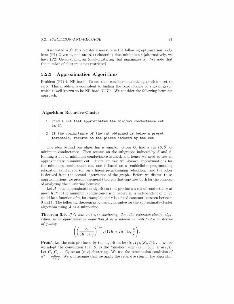
5.2. PARTITION-AND-RECURSE 71
Associated with this bicriteria measure is the following optimization prob-lem: (P1) Given α, find an (α, ε)-clustering that minimizes ε (alternatively, wehave (P2) Given ε, find an (α, ε)-clustering that maximizes α). We note thatthe number of clusters is not restricted.
5.2.3 Approximation Algorithms
Problem (P1) is NP-hard. To see this, consider maximizing α with ε set tozero. This problem is equivalent to finding the conductance of a given graphwhich is well known to be NP-hard [GJ79]. We consider the following heuristicapproach.
Algorithm: Recursive-Cluster
1. Find a cut that approximates the minimum conductance cut
in G.
2. If the conductance of the cut obtained is below a preset
threshold, recurse on the pieces induced by the cut.
The idea behind our algorithm is simple. Given G, find a cut (S, S) ofminimum conductance. Then recurse on the subgraphs induced by S and S.Finding a cut of minimum conductance is hard, and hence we need to use anapproximately minimum cut. There are two well-known approximations forthe minimum conductance cut, one is based on a semidefinite programmingrelaxation (and precurson on a linear programming relaxation) and the otheris derived from the second eigenvector of the graph. Before we discuss theseapproximations, we present a general theorem that captures both for the purposeof analyzing the clustering heuristic.
Let A be an approximation algorithm that produces a cut of conductance atmost Kxν if the minimum conductance is x, where K is independent of x (Kcould be a function of n, for example) and ν is a fixed constant between between0 and 1. The following theorem provides a guarantee for the approximate-clusteralgorithm using A as a subroutine.
Theorem 5.9. If G has an (α, ε)-clustering, then the recursive-cluster algo-rithm, using approximation algorithm A as a subroutine, will find a clusteringof quality ((
α
6K log nε
)1/ν
, (12K + 2)εν logn
ε
).
Proof. Let the cuts produced by the algorithm be (S1, T1), (S2, T2), . . ., wherewe adopt the convention that Sj is the “smaller” side (i.e., a(Sj) ≤ a(Tj)).Let C1, C2, . . . Cl be an (α, ε)-clustering. We use the termination condition ofα∗ = α
6 log nε
. We will assume that we apply the recursive step in the algorithm

72 CHAPTER 5. SPECTRAL CLUSTERING
only if the conductance of a given piece as detected by the heuristic for theminimum conductance cut is less than α∗. In addition, purely for the sake ofanalysis we consider a slightly modified algorithm. If at any point we have acluster Ct with the property that a(Ct) <
εna(V ) then we split Ct into singletons.
The conductance of singletons is defined to be 1. Then, upon termination, eachcluster has conductance at least(
α∗
K
)1/ν
=
(α
6K log nε
)1/ν
Thus it remains to bound the weight of the inter-cluster edges. Observe thata(V ) is twice the total edge weight in the graph, and so W = ε
2 a(V ) is theweight of the inter-cluster edges in this optimal solution.
Now we divide the cuts into two groups. The first group, H, consists ofcuts with “high” conductance within clusters. The second group consists ofthe remaining cuts. We will use the notation w(Sj , Tj) =
∑u∈Sj ,v∈Tj auv. In
addition, we denote by wI(Sj , Tj) the sum of the weights of the intra-cluster
edges of the cut (Sj , Tj), i.e., wI(Sj , Tj) =∑li=1 w(Sj ∩ Ci, Tj ∩ Ci). We then
set
H =j : wI(Sj , Tj) ≥ 2α∗
l∑i=1
min(a(Sj ∩ Ci), a(Tj ∩ Ci))
We now bound the cost of the high conductance group. For all j ∈ H, we have,
α∗a(Sj) ≥ w(Sj , Tj) ≥ wI(Sj , Tj) ≥ 2α∗∑i
min(a(Sj ∩ Ci), a(Tj ∩ Ci))
Consequently we observe that∑i
min(a(Sj ∩ Ci), a(Tj ∩ Ci)) ≤1
2a(Sj)
From the algorithm’s cuts, (Sj , Tj), and the optimal clustering, Ci, wedefine a new clustering via a set of cuts (S′j , T ′j) as follows. For each j ∈ H,we define a cluster-avoiding cut (S′j , T
′j) in Sj ∪Tj in the following manner. For
each i, 1 ≤ i ≤ l, if a(Sj ∩Ci) ≥ a(Tj ∩Ci), then place all of (Sj ∪ Tj)∩Ci intoS′j . If a(Sj ∩ Ci) < a(Tj ∩ Ci), then place all of (Sj ∪ Tj) ∩ Ci into T ′j .
Notice that, since |a(Sj)−a(S′j)| ≤ 12a(Sj), we have that min(a(S′j), a(T ′j)) ≥
12a(Sj). Now we will use the approximation guarantee for the cut procedure toget an upper bound on w(Sj , Tj) in terms of w(S′j , T
′j).
w(Sj , Tj)
a(Sj)≤ K
(w(S′j , T
′j)
mina(S′j), a(T ′j)
)ν
≤ K
(2w(S′j , T
′j)
a(Sj)
)ν

5.2. PARTITION-AND-RECURSE 73
Hence we have bounded the overall cost of the high conductance cuts withrespect to the cost of the cluster-avoiding cuts. We now bound the cost of thesecluster-avoiding cuts. Let P (S) denote the set of inter-cluster edges incidentat a vertex in S, for any subset S of V . Also, for a set of edges F , let w(F )denote the sum of their weights. Then, w(S′j , T
′j) ≤ w(P (S′j)), since every edge
in (S′j , T′j) is an inter-cluster edge. So we have,
w(Sj , Tj) ≤ K(2w(P (S′j))
)νa(Sj)
1−ν (5.2)
Next we prove the following claim.Claim 1. For each vertex u ∈ V , there are at most log n
ε values of j suchthat u belongs to Sj . Further, there are at most 2 log n
ε values of j such that ubelongs to S′j .
To prove the claim, fix a vertex u ∈ V . Let
Iu = j : u ∈ Sj Ju = j : u ∈ S′j \ Sj
Clearly if u ∈ Sj ∩ Sk (with k > j), then (Sk, Tk) must be a partition of Sj ora subset of Sj . Now we have, a(Sk) ≤ 1
2a(Sk ∪ Tk) ≤ 12a(Sj). So a(Sj) reduces
by a factor of 2 or greater between two successive times u belongs to Sj . Themaximum value of a(Sj) is at most a(V ) and the minimum value is at leastεna(V ), so the first statement of the claim follows.
Now suppose j, k ∈ Ju; j < k. Suppose also u ∈ Ci. Then u ∈ Tj ∩Ci. Also,later, Tj (or a subset of Tj) is partitioned into (Sk, Tk) and, since u ∈ S′k \Sk, wehave a(Tk∩Ci) ≤ a(Sk∩Ci). Thus a(Tk∩Ci) ≤ 1
2a(Sk∪Tk) ≤ 12a(Tj∩Ci). Thus
a(Tj ∩ Ci) halves between two successive times that j ∈ Ju. So, |Ju| ≤ log nε .
This proves the second statement in the claim (since u ∈ S′j implies that u ∈ Sjor u ∈ S′j \ Sj).
Using this claim, we can bound the overall cost of the group of cuts with highconductance within clusters with respect to the cost of the optimal clusteringas follows:
∑j∈H
w(Sj , Tj) ≤∑all j
K(2w(P (S′j))
)νa(Sj)
1−ν
≤ K(
2∑all j
w(P (S′j)))ν(∑
j
a(Sj))1−ν
≤ K(
2ε logn
εa(V )
)ν (2 log
n
εa(V )
)1−ν
≤ 2Kεν logn
εa(V ) (5.3)
Here we used Holder’s inequality: for real sequences a1, . . . , an and b1, . . . , bn,and any p, q ≥ 1 with (1/p) + (1/q) = 1, we have
n∑i=1
aibi ≤(
n∑i=1
api
) 1p(
n∑i=1
bqi
) 1q
.

74 CHAPTER 5. SPECTRAL CLUSTERING
Next we deal with the group of cuts with low conductance within clustersi.e., those j not in H. First, suppose that all the cuts together induce a partitionof Ci into P i1, P
i2, . . . P
iri . Every edge between two vertices in Ci which belong to
different sets of the partition must be cut by some cut (Sj , Tj) and, conversely,every edge of every cut (Sj∩Ci, Tj∩Ci) must have its two end points in differentsets of the partition. So, given that Ci has conductance α, we obtain∑all j
wI(Sj ∩ Ci, Tj ∩ Ci) =1
2
ri∑s=1
w(P is , Ci \ P is) ≥1
2α∑s
min(a(P is), a(Ci \ P is))
For each vertex u ∈ Ci there can be at most log nε values of j such that u belongs
to the smaller (according to a(·)) of the two sets Sj ∩ Ci and Tj ∩ Ci. So, wehave that
ri∑s=1
min(a(P is), a(Ci \ P is)) ≥ 1
log nε
∑j
min(a(Sj ∩ Ci), a(Tj ∩ Ci))
Thus, ∑all j
wI(Sj , Tj) ≥α
2 log nε
l∑i=1
∑j
min(a(Sj ∩ Ci), a(Tj ∩ Ci))
Therefore, from the definition of H, we have∑j /∈H
wI(Sj , Tj) ≤ 2α∗∑all j
l∑i=1
min(a(Sj ∩ Ci), a(Tj ∩ Ci)) ≤2
3
∑all j
wI(Sj , Tj)
Thus, we are able to bound the intra-cluster cost of the low conductance group ofcuts in terms of the intra-cluster cost of the high conductance group. Applying(5.3) then gives∑
j /∈H
wI(Sj , Tj) ≤ 2∑j∈H
wI(Sj , Tj) ≤ 4Kεν logn
εa(V ) (5.4)
In addition, since each inter-cluster edge belongs to at most one cut Sj , Tj , wehave that ∑
j /∈H
(w(Sj , Tj)− wI(Sj , Tj)) ≤ ε
2a(V ) (5.5)
We then sum up (5.3), (5.4) and (5.5). To get the total cost we note thatsplitting up all the Vt with a(Vt) ≤ ε
na(V ) into singletons costs us at mostε2 a(V ) on the whole. Substituting a(V ) as twice the total sum of edge weightsgives the bound on the cost of inter-cluster edge weights. This completes theproof of Theorem 5.9.
The Leighton-Rao algorithm for approximating the conductance finds a cutof conductance at most 2 log n times the minimum [LR99]. In our terminology,it is an approximation algorithm with K = 2 log n and ν = 1. Applying theorem5.9 leads to the following guarantee.

5.2. PARTITION-AND-RECURSE 75
Corollary 5.10. If the input has an (α, ε)-clustering, then, using the Leighton-Rao method for approximating cuts, the recursive-cluster algorithm finds an(
α
12 log n log nε
, 26ε log n logn
ε
)-clustering.
We now assess the running time of the algorithm using this heuristic. Thefastest implementation for this heuristic runs in O(n2) time (where the O nota-tion suppresses factors of log n). Since the algorithm makes less than n cuts, thetotal running time is O(n3). This might be slow for some real-world applica-tions. We discuss a potentially more practical algorithm in the next section. Weconclude this section with the guarantee obtained using Arora et al.’s improvedapproximation [ARV04] of O(
√log n).
Corollary 5.11. If the input to the recursive-cluster algorithm has an (α, ε)-clustering, then using the ARV method for approximating cuts, the algorithmfinds an (
α
C√
log n log nε
, Cε√
log n logn
ε
)-clustering.
where C is a fixed constant.
5.2.4 Worst-case guarantees for spectral clustering
In this section, we describe and analyze a recursive variant of the spectral algo-rithm. This algorithm, outlined below, has been used in computer vision, med-ical informatics, web search, spam detection etc.. We note that the algorithmis a special case of the recursive-cluster algorithm described in the previous sec-tion; here we use a spectral heuristic to approximate the minimum conductancecut. We assume the input is a weighted adjacency matrix A.
Algorithm: Recursive-Spectral
1. Normalize A to have unit row sums and find its second
right eigenvector v.
2. Find the best ratio cut along the ordering given by v.
3. If the value of the cut is below a chosen threshold, then
recurse on the pieces induced by the cut.
Thus, we find a clustering by repeatedly solving a one-dimensional clusteringproblem. Since the latter is easy to solve, the algorithm is efficient. The factthat it also has worst-case quality guarantees is less obvious.
We now elaborate upon the basic description of this variant of the spectralalgorithm. Initially, we normalize our matrix A by scaling the rows so that the

76 CHAPTER 5. SPECTRAL CLUSTERING
row sums are all equal to one. At any later stage in the algorithm we have apartition C1, C2, . . . , Cs. For each Ct, we consider the |Ct| × |Ct| submatrixB of A restricted to Ct. We normalize B by setting bii to 1−∑j∈Ct,j 6=i bij . Asa result, B is also non-negative with row sums equal to one.
Observe that upon normalization of the matrix, our conductance measurecorresponds to the familiar Markov Chain conductance measure i.e.
φ(S) =
∑i∈S,j 6∈S aij
min(a(S), a(S))=
∑i∈S,j 6∈S πibij
min(π(S), π(S))
where π is the stationary distribution of the Markov Chain.We then find the second eigenvector of B. This is the right eigenvector v
corresponding to the second largest eigenvalue λ2, i.e. Bv = λ2v. Then orderthe elements (rows) of Ct decreasingly with respect to their component in thedirection of v. Given this ordering, say u1, u2, . . . ur, find the minimum ratiocut in Ct. This is the cut that minimises φ(u1, u2, . . . uj, Ct) for some j,1 ≤ j ≤ r− 1. We then recurse on the pieces u1, . . . , uj and Ct \ u1, . . . , uj.
We combine Theorem 5.7 with Theorem 5.9 to get a worst-case guarantee forAlgorithm Recursive-Spectral. In the terminology of Theorem 5.9, Theorem 5.7says that the spectral heuristic for minimum conductance is an approximationalgorithm with K =
√2 and ν = 1/2.
Corollary 5.12. If the input has an (α, ε)-clustering, then, using the spectralheuristic, the approximate-cluster algorithm finds an(
α2
72 log2 nε
, 20√ε log
n
ε
)-clustering.
5.3 Discussion
The first part of this chapter is drawn partly from the work of Kumar andKannan [KK10], who analyzed the k-means algorithm after spectral projection.Their analysis was improved significantly by Awasthi and Or [AS12]. There ismuch work on the k-means algorithm and objective, and it is widely used inpractice. However, at this time, our understanding of when it can be effectivelyapplied is not complete.
The second part of this chapter is based on Kannan et al. [KVV04] andearlier work by Jerrum and Sinclair [SJ89]. Theorem 5.7 was essentially provedby Sinclair and Jerrum (in their proof of Lemma 3.3 in [SJ89], although notmentioned in the statement of the lemma). Cheng et al. [CKVW06] give anefficient implementation of recursive-spectral that maintains sparsity, and hasbeen used effectively on large data sets from diverse applications.
Spectral partitioning has also been shown to have good guarantees for somespecial classes of graphs. Notably, Spielman and Teng [ST07] proved that avariant of spectral partitioning produces small separators for bounded-degreeplanar graphs, which often come up in practical applications of spectral cuts.

5.3. DISCUSSION 77
The key contribution of their work was an upper bound on the second smallesteigenvalue of the Laplacian of a planar graph. This work was subsequentlygeneralized to graphs of bounded genus [Kel06].

78 CHAPTER 5. SPECTRAL CLUSTERING

Chapter 6
Combinatorial Optimizationvia Low-RankApproximation
79

80CHAPTER 6. COMBINATORIAL OPTIMIZATION VIA LOW-RANKAPPROXIMATION

Part II
Algorithms
81


Chapter 7
Power Iteration
Let T ∈ ⊗3Rd have an orthogonal decomposition T =∑ki=1 λivi ⊗ vi ⊗ vi with
‖vi‖ = 1 for all i ∈ [k]. For a random choice of θ ∈ Rd, for example froma spherical Gaussian, the values |λ1v
>1 θ|, |λ2v
>2 θ|, . . . , |λkv>k θ| will be distinct
with high probability.
Lemma 7.1 ([AGH+15]). Let T ∈ ⊗3Rd have an orthogonal decomposition
T =∑ki=1 λivi ⊗ vi ⊗ vi. For a vector θ0 ∈ Rd, suppose that the set of numbers
|λ1v>1 θ0|, |λ2v
>2 θ0|, . . . , |λkv>k θ0| has a unique largest element. Without loss of
generality, say |λ1v>1 θ0| is this largest value and |λ2v
>2 θ0| is the second largest
value. For t = 1, 2, . . . let
θt :=T (·, θt−1, θt−1)
‖T (·, θt−1, θt−1)‖ . (7.1)
Then
‖v1 − θt‖2 ≤(
2λ21
k∑i=2
λ−2i
)·∣∣∣∣λ2v
>2 θ0
λ1v>1 θ0
∣∣∣∣2t+1
.
That is, repeated iteration of 7.1 starting from θ0 converges to v1 at a quadraticrate.
Proof. Let v1, v2, . . . , vd be an orthonormal basis and ci = v>i θ0 for i ∈ [d], then
θ0 =∑di=1 civi. Then
θt =
∑ki=1 λ
2t−1i c2
t
i vi
‖∑ki=1 λ
2t−1i c2
t
i vi‖and
v>1 θt =λ2t−1
1 c2t
1
‖∑ki=1 λ
2t−1i c2
t
i vi‖=
1√1 +
∑ki=2
(λiciλ1c1
)2t+1 (λ1
λi
)2.
(7.2)
83

84 CHAPTER 7. POWER ITERATION
At step t,
‖v1 − θt‖2 = ‖v1‖2 + ‖θt‖2 − 2v>1 θt = 2− 2√1 +
∑ki=2
(λiciλ1c1
)2t+1 (λ1
λi
)2
≤ 2
k∑i=2
(λiciλ1c1
)2t+1 (λ1
λi
)2
≤(
2λ21
k∑i=2
λ−2i
)·∣∣∣∣λ2c2λ1c1
∣∣∣∣2t+1
.
(7.3)
For a rank ` tensor with ` > 3,
θt =
∑ki=1 λ
(`−1)t−1i c
(`−1)t
i vi
‖∑ki=1 λ
(`−1)t−1i c
(`−1)t
i vi‖.
So, the convergence rate is even faster.To apply Tensor Power Iteration to tensors obtained from moments of sam-
ples, e.g., T = E S(x ⊗ x ⊗ x), we don’t need to compute T . Rather each stepcan be implemented as
T [·, v, v] = E S(x⊗ x⊗ x)[·, v, v] =1
|S|∑xi∈S
(x>i v)2xi. (7.4)
Chapter 8
Cut decompositions
In this chapter, we study the existence and algorithms for decomposing matrices(and higher-dimensional arrays or tensors) into sums of a smaller number ofparticularly simple matrices called cut matrices. A matrix B is called a cutmatrix if there exist subsets R,C of rows and columns respectively and a realnumber b s.t.
Bij =
b if i ∈ R, j ∈ C0 otherwise.
Alternatively,B = b(1R ⊗ 1C)
where 1R is the indicator vector for the set R, defined as 1R(i) = 1 iff i ∈ R.Thus, cut matrices are rank-1 matrices with all nonzero entries being equal .A decomposition into a sum of cut matrices is called a cut decomposition. Cutdecompositions have the following properties:
• Any matrix has an “approximate” cut decomposition with a “small” num-ber of cut matrices.
• The decomposition can be found efficiently, in fact in constant time (im-plicitly) with a uniform random sample of O(1) entries from the matrix.
• The decomposition allows one to solve constraint satisfaction problemsup to additive error. This application, and classes of instances for whichthis approximation also implies a multiplicative (1 + ε) approximation, isdiscussed in the chapter on optimization using low-rank approximation.
• While the classical Singular Value Decomposition has no analog for ten-sors, cut decompositions and their approximation properties extend nat-urally to r-dimensional arrays.
In the rest of this chapter, A,B will denote m × n real matrices; S and Twill be subsets of rows and columns respectively. We let
A(S, T ) =∑
i∈S,j∈TAij .
85

86 CHAPTER 8. CUT DECOMPOSITIONS
The cut norm of a matrix A is defined as
‖A‖ = maxS,T|A(S, T )|.
Intuitively, if two matrices are close w.r.t. the cut norm, i.e., ‖A−B‖ is small,then on every cut the sum of their entries is approximately equal. In Chapter??, we study applications of cut decompositions to combinatorial optimization.
8.1 Existence of small cut decompositions
We begin with a proof of existence of a good cut decomposition for any matrix.
Lemma 8.1. Let A ∈ Rm×n. For any ε > 0, there exist t ≤ 1/ε2 cut matricesB1, . . . , Bt whose sum B =
∑ti=1Bt satisfies
‖A−B‖ ≤ ε√mn‖A‖F .
We note that if |Aij | ≤ 1 for all i, j, then the upper bound is εmn. Moreover,the inequality above is tight with the cut norm on the LHS and the Frobeniusnorm on the RHS (i.e., we cannot get the same norm on both sides).
Exercise 8.1. Let a1, a2, . . . , an be real numbers and a be their average. Definebi = ai − a. Show that
n∑i=1
b2i ≤n∑i=1
a2i .
Proof. (of Lemma 8.1). If ‖A‖ ≤ ε√mn‖A‖F , we take B = 0. Otherwise, for
some S, T such that
|A(S, T )| > ε√mn‖A‖F .
Define B1 to be the cut matrix defined by these subsets S, T with
(B1)ij =A(S, T )
|S||T |
for all (i, j) ∈ S × T and zero elsewhere. Now consider the Frobenius norm ofA−B1
‖A−B1‖2F = ‖A‖2F − ‖B1‖2F≤ ‖A‖2F − ε2
mn
|S||T | ‖A‖2F
≤ ‖A‖2F − ε2‖A‖2F .
We recurse on the matrix A − B1 using the same condition on the cut norm.Since each step reduces the squared Frobenius norm by ε2 times the initial value,it must terminate in at most 1/ε2 steps.

8.2. CUT DECOMPOSITION ALGORITHM 87
8.2 Cut decomposition algorithm
How quickly can one find a cut decomposition of a given matrix with the approx-imation property asserted in Lemma 8.1? In principle, this is a combinatorialproblem with exponentially many candidates. From the proof of the Lemma(8.1), we see that it suffices to determine if the cut norm of A is at most εmnand if not, to find an S, T with |A(S, T )| ≥ εmn. Computing the cut norm isNP-hard. However, to recover the cut decomposition guarantee, an approximateversion suffices: find the maximum value of |A(S, T )| to within additive error(ε/2)mn. This reduces to two problems: maxA(S, T ) and max−A(S, T ). Wedescribe now an efficient algorithm for computing maxA(S, T ); we call this theMaximum submatrix problem.
For a subset of rows S, we observe that a subset of columns T that maximizesA(S, T ) is easy to compute, namely,
T = j : A(S, j) > 0.
We will make use of this simple observation in the algorithm.
Algorithm: Max-Submatrix
1. Pick a subset W of s rows uniformly at random.
2. For every subset W of W, find the set of columns Twhose sum in the W rows is positive.
3. For each candidate T, let S be the rows with positive
sum in the T columns.
4. Among all candidate S, T enumerated above, output the
subsets that achieve maxA(S, T ).
The idea behind the algorithm is the following: we guess a small randomsubset of the optimal subset of rows S, then use this small subset to approxi-mately identify the columns with positive sums. A small random subset shouldsuffice since this will suffice to identify columns with significant sums, and theones with sums close to zero are relatively unimportant. We guess such a subsetby first picking a random subset of rows W of the full matrix and enumeratingall possibilities for S ∩W , i.e., all subsets of W . In the estimating column sumsstep, if we had the correct S ∩ W , (which will happen at some point in theenumeration) the only columns on which we could be wrong about the sign ofthe column sum in the S rows are ones where the column sum is close to zero,and these do not contribute significantly to A(S, T ). So, one of our candidatesT is approximately the best one in the sense that A(S, T ) is high for the optimalrow subset S.
Now we turn to a rigorous analysis of the algorithm. It is easy to see that therunning time of the algorithm is O(mn2s). Setting s = 16/ε2, the next theorem

88 CHAPTER 8. CUT DECOMPOSITIONS
recovers the additive guarantee of the existence lemma in time O(mn2s) =
O(mn216/ε2). In the next section, we will see how the running time can befurther improved.
Theorem 8.2. With probability at least 1− δ, the subsets S, T found by Algo-rithm Max-Submatrix we satisfy
A(S′, T ′) ≥ A(S∗, T ∗)− 1
δ
√mn
s‖A‖F
where S∗, T ∗ is an optimal solution.
The proof of this theorem relies on the following lemma.
Lemma 8.3. Suppose A is an m× n matrix. Fix a subset S of rows of A. LetT be the set of columns with positive sum in the S rows. Let W be a uniformrandom subset of rows of cardinality s and T be the set of columns with positivesum in the W ∩ S rows. Then,
E W (A(S, T )) ≥ A(S, T )−√mn
s‖A‖F . (8.1)
The following lemma will be useful in the proof.
Lemma 8.4. Let X1, . . . , Xn be i.i.d. random variables from some distribu-tion and Y1, . . . , Yn be random variables from the same distribution but withoutreplacement, i.e., Yj is drawn from the original distribution restricted to thecomplement of Y1, . . . , Yj−1. Then for any convex function φ : R→ R,
E (φ(
n∑i=1
Yi)) ≤ E (φ(
n∑i=1
Xi)).
Proof. (of Lemma 8.3). We write
A(S, T ) = A(S, T )−A(S,B1) +A(S,B2), (8.2)
where
B1 = j : A(S, j) > 0 and A(S ∩W, j) ≤ 0,B2 = j : A(S, j) ≤ 0 and A(S ∩W, j) > 0.
Let a(j) =∑i∈S A
2ij ,
Xj = A(S ∩W, j) =∑i∈S
Aij1W (i)
where 1W is the indicator vector of the subset W . Therefore,
E (Xj) =s
mA(S, j).

8.2. CUT DECOMPOSITION ALGORITHM 89
To bound the variance we will use Lemma 8.4 with the convex function φ(x) =x2.
Var (Xj) ≤ E ((∑i∈S
Aij1W (i))2) ≤ s
ma(j).
Hence, for any t ≥ 0, using Chebychev’s inequality,
Pr(∣∣∣Xj −
s
mA(S, j)
∣∣∣ ≥ t) ≤ sa(j)
mt2(8.3)
If j ∈ B1 then
Xj −s
mA(S, j) ≤ − s
mA(S, j)
and so applying (8.3) with
t =s
mA(S, j),
we get that for each fixed j,
Pr(j ∈ B1) ≤ ma(j)
sA(S, j)2.
Thus,
E
∑j∈B1
A(S, j)
≤∑
j: A(S,j)>0
min
A(S, j),
ma(j)
sA(S, j)
≤∑
j: A(S,j)>0
√ma(j)
s(8.4)
By an identical argument we obtain
E
∑j∈B2
A(S, j)
≥ − ∑j: A(S,j)<0
√ma(j)
s.
Hence, using Cauchy-Schwartz,
E (A(S, T )) ≥ A(S, T )−∑j
√ma(j)
s≥ A(S, T )−
√mn
s‖A‖F .
We conclude this section with a proof of the main guarantee for the algo-rithm.
Proof. (of Theorem 8.2.) Let S∗, T ∗ = arg maxA(S, T ) where the maximum isover all choices of subsets S, T . Let S, T be the subsets found by the algorithm.Applying Lemma 8.3 to S∗, T ∗, we have
E (A(S, T )) ≥ A(S∗, T ∗)−√mn
s‖A‖F .

90 CHAPTER 8. CUT DECOMPOSITIONS
Alternatively,
E (A(S∗, T ∗)−A(S, T )) ≤√mn
s‖A‖F .
Applying Markov’s inequality, for any 0 ≤ δ ≤ 1,
Pr(A(S∗, T ∗)−A(S, T ) ≥ 1
δ
√mn
s‖A‖F ) ≤ δ.
In other words, with probability at least 1− δ,
A(S, T ) ≥ A(S∗, T ∗)− 1
δ
√mn
s‖A‖F .
8.3 A constant-time algorithm
In this section, we extend Algorithm Max-Submatrix so that in constant time,it finds an implicit representation of S, T that approximately maximize A(S, T ).By constant time we mean a time bound that depends only on ε and not onm,n.
The idea is simple: Pick uniform random subsets S of s = O(1/ε4) rows andT of s columns at the outset. Instead of A, we use this sampled submatrix forall row and column sum estimates, i.e., we estimate A(S, T ) by
mn
s2A(S ∩ S, T ∩ T ),
for which we only need to know the entries of A in S × T . One can show usingthe Hoffding-Azuma inequality that the estimate is within additive error at mostO(εmn) with high probability.
Theorem 8.5. For A with |Aij | ≤ 1, for any fixed ε > 0, Algorithm Max-Submatrix executed with s = O(1/ε2) on a random submatrix of A induced by srandom rows and s random columns of A finds S, T such that with probabilityat least 3/4,
|maxA(S, T )− mn
s2A(S, T )| ≤ 16mn√
s.
Moreover, the running time to find S, T , from which the approximately optimalS, T can be found is 2s. A full cut-decomposition B with the guarantees ofLemma 8.1 can be implicitly computed in time O(s32s).
Thus, the value of maxA(S, T ) can be estimated in constant time indepen-dent of m,n.

8.4. CUT DECOMPOSITIONS FOR TENSORS 91
Exercise 8.2. Prove Theorem 8.5 for s = O(1/ε4), by showing that with prob-ability at least 7/8, for every T ⊂ T ,
|A(S, T )− mn
s2A(S ∩ S, T ∩ T )| ≤ εmn.
[Hint: use the Hoeffding-Azuma inequality for any candidate T and apply aunion bound. The inequality says that given random variables X1, . . . , Xn with|Xi| ≤ 1 and E (Xi|X1, . . . , Xi−1) = 0 for all i ∈ [n], their sum X satisfies
Pr(|X − E (X)| ≥ t) ≤ 2e−t2
2n .]
8.4 Cut decompositions for tensors
We next consider r-dimensional tensors, i.e., A ∈ Rn1×n2×...×nr . For subsetsS1 ⊆ [n1], . . . , Sr ⊆ [nr] of the indices, we can define A(S1, . . . , Sr) as the sumof all entries in the induced subtensor. The cut norm generalizes as follows:
‖A‖ = max |A(S1, . . . , Sr)|.A cut tensor is tensor defined by a subsets of indices S1, . . . , Sr, with Ai1,...,irbeing a constant if (i1, . . . , ir) ∈ S1 × . . .× Sr and zero otherwise. A cut tensoris thus a rank-one tensor obtained as the outer product of r vectors with entriesfrom 0, 1. The existence of cut decompositions is captured in the next exercise.
Exercise 8.3. Show that Lemma 8.1 extends to r-dimensional tensors for anyr, i.e., if A ∈ Rn1×n2×...×nr , for any ε > 0, there exist t ≤ 1/ε2 cut tensorsB1, . . . , Bt s.t. their sum B =
∑ti=1Bi satisfies
‖A−B‖ ≤ ε√n1n2 . . . nr‖A‖F .
The idea for solving the maximum subtensor problem to within additiveerror is the following. First we observe that given subsets S1, . . . , Sr−1, we canfind the optimal subset Sr ⊆ [nr] as the subset of indices with positive sums,i.e., i s.t. A(S1, . . . , Sr−1, i) is positive. Using this,
1. We fix random subsets W1,W2, . . . ,Wr−1 each of size s.
2. We enumerate all possible subsets Wt ⊆Wt as candidates for St∩Wt. Foreach such candidate W1, . . . , Wr−1, we find the best subset Sr.
3. For each Sr, we form the (r − 1)-tensor A as
Ai1i2...ir−1=∑i∈Sr
Ai1i2...ir−1i
and recursively solve the maximum subtensor problem for this r−1 tensor.
4. Among all the candidates enumerated, choose the best Sr.
Exercise 8.4. Show that in order to achieve the guarantee of Exercise 8.3 withhigh probability, it suffices to set s = poly(r, 1/ε).

92 CHAPTER 8. CUT DECOMPOSITIONS
8.5 A weak regularity lemma
In this section, we study a variant of the regularity lemma from graph theory.We first briefly recall Szemeredi’s original lemma.
Let G be an undirected graph on n vertices. For a pair of subset of verticesA,B, let e(A,B) be the number of edges between A and B (A and B couldintersect). The density of a pair A,B is
d(A,B) =e(A,B)
|A||B| .
A pair of subsets V1, V2 ⊆ V is said to be ε-regular if for any two subsetsA ⊆ V1, B ⊆ V2,
|d(A,B)− d(V1, V2)| ≤ ε.
A partition of V into k subsets is called an ε-regular partition if all but εk2 pairsof subsets are ε-regular.
Theorem 8.6 (Regularity). For any ε > 0, there exists k = k(ε), such that forany graph G there is an ε-regular partition with at most k parts.
The theorem can be further strengthened by noting that no part is too largeand the part sizes are comparable. This powerful theorem has many applicationsin combinatorics, analysis and computer science. Unfortunately, the functionk(ε) is a tower function of height 1/ε and such a dependence is unavoidable ingeneral.
The weak regularity lemma, which we state next, follows from cut decom-positions and has a much smaller bound on the size of a partition, albeit witha weaker guarantee.
Theorem 8.7 (Weak Regularity). For any ε > 0, and any graph G, there exists
a partition of the vertices of G into k ≤ 22/ε2 parts such that for any two subsetS, T ⊆ V , ∣∣∣∣∣∣e(S, T )−
k∑i,j=1
d(Vi, Vj)|S ∩ Vi||T ∩ Vj |)|
∣∣∣∣∣∣ ≤ εn2.
Such a parition is called an ε-pseudo-regular partition of the graph.
Proof. Let B1, . . . , Bs be a cut decomposition of the adjacency matrix of G.Consider the partition induced by the subsets R1, . . . , Rs, T1, . . . , Ts of size k ≤22s. The matrix B = B1 + . . . + Bs can be partitioned into a sum of k cutmatrices with disjoint support so that B is their sum. Moreoever the value ofeach cut matrix is simply its density in the original graph. This completes theproof.

8.6. DISCUSSION 93
8.6 Discussion
SzemerediNesterov, Alon-Naor Grothendieck approximationsCut decompositions were introduced by Frieze and Kannan [FK99].Graph limits

94 CHAPTER 8. CUT DECOMPOSITIONS

Chapter 9
Matrix approximation byRandom Sampling
In this chapter, we study randomized algorithms for matrix multiplication andlow-rank matrix and tensor approximation. The main motivation is to obtainefficient approximations using only randomly sampled subsets of given matrices.We remind the reader that for a vector-valued random variable X, we writeVar (X) = E (‖X−E (X)‖2) and similarly for a matrix-valued random variable,with the norm denoting the Frobenius norm in the latter case.
9.1 Matrix-vector product
In many numerical algorithms, a basic operation is the matrix-vector product.If A is a m × n matrix and v is an n vector, we have (A(j) denotes the j’thcolumn of A):
Av =
n∑j=1
A(j)vj .
The right-hand side is the sum of n vectors and can be estimated by using asample of the n vectors. The error is measured by the variance of the estimate.It is easy to see that a uniform random sample could have high variance —consider the example when only one column is nonzero.
This leads to the question: what distribution should the sample columns bechosen from? Let p1, p2, . . . pn be nonnegative reals adding up to 1. Pick j ∈1, 2, . . . n with probability pj and consider the vector-valued random variable
X =A(j)vjpj
.
95

96 CHAPTER 9. MATRIX APPROXIMATION BY RANDOM SAMPLING
Clearly E X = Av, so X is an unbiased estimator of Av. We also get
Var (X) = E ‖X‖2 − ‖E X‖2 =
n∑j=1
‖A(j)‖2v2j
pj− ‖Av‖2. (9.1)
Now we introduce an important probability distribution on the columns of amatrix A, namely the length-squared (LS) distribution, where a column ispicked with probability proportional to its squared length. We will say
j is drawn from LScol(A) if pj = ‖A(j)‖2/‖A‖2F .This distribution has useful properties. An approximate version of this distri-bution - LScol(A, c), where we only require that
pj ≥ c‖A(j)‖2/‖A‖2Ffor some c ∈ (0, 1) also shares interesting properties. If j is from LScol(A, c),then note that the expression (9.1) simplifies to yield
Var X ≤ 1
c‖A‖2F ‖v‖2.
Taking the average of s i.i.d. trials decreases the variance by a factor of s. So,if we take s independent samples j1, j2, . . . js (i.i.d., each picked according toLScol(A, c)), then with
Y =1
s
s∑t=1
A(jt)vjtpjt
,
we haveE Y = Av
and
Var Y =1
s
∑j
‖A(j)‖2v2j
pj− 1
s‖Av‖2 ≤ 1
cs‖A‖2F ‖v‖2. (9.2)
Such an approximation for matrix vector products is useful only when ‖Av‖is comparable to ‖A‖F ‖v‖. It is greater value for matrix multiplication.
In certain contexts, it may be easier to sample according to LS(A, c) thanthe exact length squared distribution. We have used the subscript col to denotethat we sample columns of A; it will be sometimes useful to sample rows, againwith probabilities proportional to the length squared (of the row, now). In thatcase, we use the subscript row.
9.2 Matrix Multiplication
The next basic problem is that of multiplying two matrices, A,B, where A ism× n and B is n× p. From the definition of matrix multiplication, we have
AB =(AB(1), AB(2), . . . AB(p)
).

9.3. LOW-RANK APPROXIMATION 97
Applying (9.2) p times and adding, we get the next theorem (recall the notationthat B(j) denotes row j of B).
Theorem 9.1. Let p1, p2, . . . pn be non-negative reals summing to 1 and letj1, j2, . . . js be i.i.d. random variables, where jt is picked to be one of 1, 2, . . . nwith probabilities p1, p2, . . . pn respectively. Then with
Y =1
s
s∑t=1
A(jt)B(jt)
pjt,
E Y = AB and Var Y =1
s
n∑j=1
‖A(j)‖2‖B(j)‖2pj
− ‖AB‖2F .(9.3)
If jt are distributed according to LScol(A, c), then
Var Y ≤ 1
cs‖A‖2F ‖B‖2F .
A special case of matrix multiplication which is both theoretically and prac-tically useful is the product AAT .
The singular values of AAT are just the squares of the singular values of A.So it can be shown that if B ≈ AAT , then the eigenvalues of B will approximatethe squared singular values of A. Later, we will want to approximate A itselfwell. For this, we will need in a sense a good approximation to not only thesingular values, but also the singular vectors of A. This is a more difficultproblem. However, approximating the singular values well via AAT will be acrucial starting point for the more difficult problem.
For the matrix product AAT , the expression for Var Y (in (9.3)) simplifiesto
Var Y =1
s
∑j
‖A(j)‖4pj
− ‖AAT ‖2F .
The second term on the right-hand side is independent of pj . The first term isminimized when the pj conform to the length-squared distribution.
9.3 Low-rank approximation
When B = AT , we may rewrite the expression (9.3) as
Y = CCT , where, C =1√s
(A(j1)
√pj1
,A(j2)
√pj2
, . . .A(js)
√pjs
)and the next theorem follows.
Theorem 9.2. Let A be an m×n matrix and j1, j2, . . . js be i.i.d. samples from1, 2, . . . n, each picked according to probabilities p1, p2, . . . pn. Define
C =1√s
(A(j1)
√pj1
,A(j2)
√pj2
, . . .A(js)
√pjs
).

98 CHAPTER 9. MATRIX APPROXIMATION BY RANDOM SAMPLING
Then,
E CCT = AAT and E ‖CCT −AAT ‖2F =1
s
n∑j=1
|A(j)|4pj
− 1
s‖AAT ‖2F .
If the pj’s conform to the approximate length squared distribution LScol(A, c),then
E ‖CCT −AAT ‖2F ≤1
cs‖A‖4F .
The fact that ‖CCT −AAT ‖F is small implies that the singular values of Aare close to the singular values of C. Indeed the Hoffman-Wielandt inequalityasserts that ∑
t
(σt(CC
T )− σt(AAT ))2 ≤ ‖CCT −AAT ‖2F . (9.4)
(Exercise 9.3 asks for a proof of this inequality.)To obtain a good low-rank approximation of A, we will also need a handle
on the singular vectors of A. A natural question is whether the columns of Calready contain a good low-rank approximation to A. To this end, first observethat if u(1), u(2), . . . u(k) are orthonormal vectors in Rm, then
k∑t=1
u(t)u(t)TA
is the projection of A into the space H spanned by u(1), u(2), . . . u(k), namely
(i) For any u ∈ H, uTA = uT∑kt=1 u
(t)u(t)TA and
(ii) For any u ∈ H⊥, uT∑kt=1 u
(t)u(t)TA = 0.
This motivates the following algorithm for low-rank approximation.
Algorithm: Fast-SVD
1. Sample s columns of A from the squared length
distribution to form a matrix C.
2. Find u(1), . . . , u(k), the top k left singular vectors of C.
3. Output∑kt=1 u
(t)u(t)TA as a rank-k approximation to A.
The running time of the algorithm (if it uses s samples) is O(ms2).We now state and prove the main lemma of this section. Recall that Ak
stands for the best rank-k approximation to A (in Frobenius norm and 2-norm)and is given by the first k terms of the SVD.

9.3. LOW-RANK APPROXIMATION 99
Lemma 9.3. Suppose A,C are m × n and m × s matrices respectively withs ≤ n and U is the m× k matrix consisting of the top k singular vectors of C.Then,
‖A− UUTA‖2F ≤ ‖A−Ak‖2F + 2√k‖AAT − CCT ‖F
‖A− UUTA‖22 ≤ ‖A−Ak‖22 + ‖CCT −AAT ‖2 + ‖CCT −AAT ‖F .Proof. We have
‖A−k∑t=1
u(t)u(t)TA‖2F = ‖A‖2F − ‖UTA‖2F
and‖Ck‖2F = ‖UTC‖2F .
Using these equations,
‖A−k∑t=1
u(t)u(t)TA‖2F − ‖A−Ak‖2F
= ‖A‖2F − ‖UTA‖2F − (‖A‖2F − ‖Ak‖2F )
=(‖Ak‖2F − ‖Ck‖2F
)+ ‖UTC‖2F − ‖UTA‖2F
=
k∑t=1
(σt(A)2 − σt(C)2
)+
k∑t=1
(σt(C)2 − ‖u(t)TA‖2
)
≤
√√√√k
k∑t=1
(σt(A)2 − σt(C)2)2
+
√√√√k
k∑t=1
(σt(C)2 − ‖u(t)TA‖2
)2
=
√√√√k
k∑t=1
(σt(AAT )− σt(CCT ))2
+
√√√√k
k∑t=1
(u(t)T (CCT −AAT )u(t)
)2
≤ 2√k‖AAT − CCT ‖F .
Here we first used the Cauchy-Schwarz inequality on both summations and thenthe Hoffman-Wielandt inequality 9.4.
The proof of the second statement also uses the Hoffman-Wielandt inequal-ity.
Exercise 9.1. Prove the 2-norm bound in the statement of Lemma 9.3.
We can now combine Theorem 9.2 and Lemma 9.3 to obtain the main the-orem of this section.
Theorem 9.4. Algorithm Fast-SVD finds a rank-k matrix A such that
E(‖A− A‖2F
)≤ ‖A−Ak‖2F + 2
√k
s‖A‖2F
E(‖A− A‖22
)≤ ‖A−Ak‖2 +
2√s‖A‖2F .

100CHAPTER 9. MATRIX APPROXIMATION BY RANDOM SAMPLING
Exercise 9.2. Using the fact that ‖A‖2F = Tr(AAT ) show that:
1. For any two matrices P,Q, we have |TrPQ| ≤ ‖P‖F ‖Q‖F .
2. For any matrix Y and any symmetric matrix X, |TrXYX| ≤ ‖X‖2F ‖Y ‖F .
Exercise 9.3. Prove the Hoffman-Wielandt inequality for symmetric matrices:for any two n× n symmetric matrices A and B,
n∑t=1
(σt(A)− σt(B))2 ≤ ‖A−B‖2F .
(Hint: consider the SVD of both matrices and note that any doubly stochasticmatrix is a convex combination of permutation matrices).
Exercise 9.4. (Sampling on the fly) Suppose you are reading a list of realnumbers a1, a2, . . . an in a streaming fashion, i.e., you only have O(1) memoryand the input data comes in arbitrary order in a stream. Your goal is to outputa number X between 1 and n such that:
Pr(X = i) =a2i∑n
j=1 a2j
.
How would you do this? How would you pick values for X1, X2, . . . Xs (s ∈ O(1))where the Xi are i.i.d.?
In this section, we considered projection to the span of a set of orthogonalvectors (when the u(t) form the top k left singular vectors of C). In the nextsection, we will need to deal also with the case when the u(t) are not orthonormal.A prime example we will deal with is the following scenario: suppose C is anm× s matrix, for example obtained by sampling s columns of A as above. Nowsuppose v(1), v(2), . . . v(k) are indeed an orthonormal set of vectors for which
C ≈ C∑kt=1 v
(t)v(t)T ; i.e.,∑kt=1 v
(t)v(t)T is a “good right projection” space forC. Then suppose the u(t) are defined by u(t) = Cv(t)/|Cv(t)|. We will see later
that C ≈ ∑kt=1 u
(t)u(t)TC; i.e., that∑kt=1 u
(t)u(t)T is a good left projectionspace for C. The following lemma which generalizes some of the arguments wehave used here will be useful in this regard.
Lemma 9.5. Suppose u(1), u(2), . . . u(k) are any k vectors in Rm. SupposeA,C are any two matrices, each with m rows (and possibly different numbers of

9.3. LOW-RANK APPROXIMATION 101
columns.) Then, we have
‖A−k∑t=1
u(t)u(t)TA‖2F − ‖C −k∑t=1
u(t)u(t)TC‖2F
≤ ‖A‖2F − ‖C‖2F
+ ‖AAT − CCT ‖F ‖k∑t=1
u(t)u(t)T ‖F(
2 + ‖k∑t=1
u(t)u(t)T ‖F)
(9.5)
‖A−k∑t=1
u(t)u(t)TA‖22 − ‖C −k∑t=1
u(t)u(t)TC‖22
≤ ‖AAT − CCT ‖2(‖
k∑t=1
u(t)u(t)T ‖2 + 1
)2
. (9.6)
Proof.
‖A−k∑t=1
u(t)u(t)TA‖2F
= Tr
((A−
k∑t=1
u(t)u(t)TA)(AT −ATk∑t=1
u(t)u(t)T )
)
= TrAAT + Tr
k∑t=1
u(t)u(t)TAATk∑t=1
u(t)u(t)T − 2Tr
k∑t=1
u(t)u(t)TAAT ,
where we have used the fact that square matrices commute under trace. We dothe same expansion for C to get
‖A−k∑t=1
u(t)u(t)TA‖2F − ‖C −k∑t=1
u(t)u(t)TC‖2F −(‖A‖2F − ‖C‖2F
)= Tr
k∑t=1
u(t)u(t)T (AAT − CCT )
k∑t=1
u(t)u(t)T − 2Tr
k∑t=1
u(t)u(t)T (AAT − CCT )
≤ ‖k∑t=1
u(t)u(t)T ‖2F ‖AAT − CCT ‖F + 2‖k∑t=1
u(t)u(t)T ‖F ‖AAT − CCT ‖F ,
where we have used two standard inequalities: |TrPQ| ≤ ‖P‖F ‖Q‖F for anymatrices P,Q and |TrXYX| ≤ ‖X‖2F ‖Y ‖F for any Y and a symmetric matrixX (see Exercise 9.2). This gives us (9.5).
For (9.6), suppose v is the unit length vector achieving
‖vT (A−k∑t=1
u(t)u(t)TA)‖ = ‖A−k∑t=1
u(t)u(t)TA‖2.

102CHAPTER 9. MATRIX APPROXIMATION BY RANDOM SAMPLING
Then we expand
‖vT (A−k∑t=1
u(t)u(t)TA)‖2
= vT (A−k∑t=1
u(t)u(t)TA)(AT −ATk∑t=1
u(t)u(t)T )v
= vTAAT v − 2vTAATk∑t=1
u(t)u(t)T v + vTk∑t=1
u(t)u(t)TAATk∑t=1
u(t)u(t)T v,
and the corresponding terms for C. Now, (9.6) follows by a somewhat tediousbut routine calculation.
9.3.1 A sharper existence theorem
In this section, we establish the existence of a rank k approximation of anymatrix A in the span of a small sample of columns from LScol(A). The boundwill be better than the one achieved in the algorithm above, namely for additiveerror ε‖A‖2F , one needs only O(k/ε) columns rather than O(k/ε2) columns. Wewill see later that this bound is asymptotically optimal.
Theorem 9.6. Let S be an i.i.d. sample of s columns from LScol(A). Thereexists a matrix A of rank at most k, with columns in the span of S s.t.,
E (‖A− A‖2F ) ≤ ‖A−Ak‖2F +k
s‖A‖2F
E (‖A− A‖22) ≤ ‖A−Ak‖22 +1
s‖A‖2F
where Ak is the best rank-k approximation of A as given by its SVD.
9.4 Invariant subspaces
The classical SVD has associated with it the decomposition of space into thesum of invariant subspaces.
Theorem 9.7. Let A be a m× n matrix and v(1), v(2), . . . v(n) an orthonormalbasis for Rn. Suppose for k, 1 ≤ k ≤ rank(A) we have
|Av(t)|2 = σ2t (A), for t = 1, 2, , . . . k.
Then
u(t) =Av(t)
|Av(t)| , for t = 1, 2, . . . k

9.4. INVARIANT SUBSPACES 103
form an orthonormal family of vectors. The following hold:
k∑t=1
|u(t)TA|2 =
k∑t=1
σ2t
‖A−Ak∑t=1
v(t)v(t)T ‖2F = ‖A−k∑t=1
u(t)u(t)TA‖2F
=
n∑t=k+1
σ2t (A)
‖A−Ak∑t=1
v(t)v(t)T ‖2 = ‖A−k∑t=1
u(t)u(t)TA‖2 = σk+1(A).
Given the right singular vectors v(t), a family of left singular vectors u(t)
may be found by just applying A to them and scaling to length 1. The orthog-onality of the u(t) is automatically ensured. So we get that given the optimal
k dimensional “right projection” A∑kt=1 v
(t)v(t)T , we also can get the optimal“left projection”
k∑t=1
u(t)u(t)TA.
Counting dimensions, it also follows that for any vector w orthogonal to sucha set of v(1), v(2), . . . v(k), we have that Aw is orthogonal to u(1), u(2), . . . u(k).This yields the standard decomposition into the direct sum of subspaces.
Exercise 9.5. Prove Theorem 9.7.
We now extend the previous theorem to approximate invariance, i.e., even ifthe hypothesis of the previous theorem |Av(t)|2 = σ2
t (A) is only approximatelysatisfied, an approximate conclusion follows. We give below a fairly clean state-ment and proof formalizing this intuition. It will be useful to define the errormeasure
∆(A, v(1), v(2), . . . v(k)) = Max1≤t≤k
t∑i=1
(σ2i (A)− |Av(i)|2). (9.7)
Theorem 9.8. Let A be a matrix of rank r and v(1), v(2), . . . v(r) be an or-thonormal set of vectors spanning the row space of A (so that Av(t) span thecolumn space of A). Then, for t, 1 ≤ t ≤ r, we have
r∑s=t+1
(v(t)TATAv(s)
)2
≤ |Av(t)|2(σ2
1(A) + σ22(A) + . . . σ2
t (A)− |Av(1)|2 − |Av(2)|2 − . . . |Av(t)|2).

104CHAPTER 9. MATRIX APPROXIMATION BY RANDOM SAMPLING
Note that v(t)TATAv(s) is the (t, s) th entry of the matrix ATA when written
with respect to the basis v(t). So, the quantity∑rs=t+1
(v(t)TATAv(s)
)2
is
the sum of squares of the above diagonal entries of the t th row of this matrix.Theorem (9.8) implies the classical Theorem (9.7) : σt(A) = |Av(t)| implies that
the right hand side of the inequality above is zero. Thus, v(t)TATA is colinear
with v(t)T and so |v(t)TATA| = |Av(t)|2 and so on.
Proof. First consider the case when t = 1. We haver∑s=2
(v(1)TATAv(s))2 = |v(1)TATA|2 − (v(1)TATAv(1))2
≤ |Av(1)|2σ1(A)2 − |Av(1)|4≤ |Av(1)|2(σ1(A)2 − |Av(1)|2). (9.8)
The proof of the theorem will be by induction on the rank of A. If r = 1, thereis nothing to prove. Assume r ≥ 2. Now, Let
A′ = A−Av(1)v(1)T .
A′ is of rank r− 1. If w(1), w(2), . . . are the right singular vectors of A′, they areclearly orthogonal to v(1). So we have for any s, 1 ≤ s ≤ r − 1,
σ21(A′) + σ2
2(A′) + . . . σ2s(A′) =
s∑t=1
|A′w(t)|2 =
s∑t=1
|Aw(t)|2
= |Av(1)|2 +
s∑t=1
|Aw(t)|2 − |Av(1)|2
≤ maxu(1),u(2)...u(s+1) orthonormal
s+1∑t=1
|Au(t)|2 − |Av(1)|2
= σ1(A)2 + σ2(A)2 + . . . σs+1(A)2 − |Av(1)|2, (9.9)
where we have applied the fact that for any k, the k-dimensional SVD subspacemaximizes the sum of squared projections among all subspaces of dimension atmost k.
Now, we use the inductive assumption on A′ with the orthonormal basisv(2), v(3), . . . v(r). This yields for t, 2 ≤ t ≤ r,
r∑s=t+1
(v(t)TA′TA′v(s))2
≤ |A′v(t)|2(σ21(A′) + σ2
2(A′) + . . . σ2t−1(A′)− |A′v(2)|2 − |A′v(3)|2 − . . . |A′v(t)|2)
Note that for t ≥ 2, we have A′v(t) = Av(t). So, we get using (9.9)
r∑s=t+1
(v(t)TATAv(s))2
≤ |Av(t)|2(σ21(A) + σ2
2(A) + . . . σ2t (A)− |Av(1)|2 − |Av(2)|2 − . . . |Av(t)|2).

9.4. INVARIANT SUBSPACES 105
This together with (9.8) finishes the proof of the Theorem.
We will use Theorem (9.8) to prove Theorem (9.9) below. Theorem (9.9)says that we can get good “left projections” from “good right projections”. Oneimportant difference from the exact case is that now we have to be more carefulof “near singularities”, i.e. the upper bounds in the Theorem (9.9) will dependon a term
k∑t=1
1
|Av(t)|2 .
If some of the |Av(t)| are close to zero, this term is large and the bounds canbecome useless. This is not just a technical problem. In defining u(t) in Theorem(9.7) as Av(t)/|Av(t)|, the hypotheses exclude t for which the denominator iszero. Now since we are dealing with approximations, it is not only the zerodenominators that bother us, but also small denominators. We will have toexclude these too (as in Corollary (9.10) below) to get a reasonable bound.
Theorem 9.9. Suppose A is a matrix and v(1), . . . v(k) are orthonormal and let∆ = ∆(A, v(1), v(2), . . . v(k)) be as in (9.7). Let
u(t) =Av(t)
|Av(t)| for t = 1, 2, . . . k.
Then
‖k∑t=1
u(t)u(t)TA−A‖2F ≤ ‖A−k∑t=1
Av(t)v(t)T ‖2F
+
(k∑t=1
2
|Av(t)|2
)(k∑t=1
|Av(t)|2)
∆
‖k∑t=1
u(t)u(t)TA−A‖22 ≤ ‖A−k∑t=1
Av(t)v(t)T ‖22
+
(k∑t=1
2
|Av(t)|2
)(k∑t=1
|Av(t)|2)
∆.
Proof. Complete v(1), v(2), . . . v(k) to an orthonormal set v(1), v(2), . . . v(r)such that Av(t) : t = 1, 2, . . . r span the range of A. Let
w(t)T = v(t)TATA− |Av(t)|2v(t)T
be the component of v(t)TATA orthogonal to v(t)T . We have
u(t)u(t)TA =Av(t)v(t)TATA
|Av(t)|2 = Av(t)v(t)T +Av(t)w(t)T .
106CHAPTER 9. MATRIX APPROXIMATION BY RANDOM SAMPLING
Using ||X + Y ||2F = Tr((XT + Y T )(X + Y )) = ||X||2F + ||Y ||2F + 2TrXTY andthe convention that t runs over 1, 2, . . . k, we have
||∑t
u(t)u(t)TA−A||2F =
∣∣∣∣∣∣∣∣∣∣∑t
Av(t)v(t)T +∑t
Av(t)w(t)T
|Av(t)|2 −A∣∣∣∣∣∣∣∣∣∣2
F
= ||A−∑t
Av(t)v(t)T ||2F +
(∑t
∣∣∣∣ Av(t)
|Av(t)|2∣∣∣∣ ∣∣∣w(t)
∣∣∣)2
−2
r∑s=1
∑t
(v(s)Tw(t))v(t)TAT
|Av(t)|2 (A−∑t
Av(t)v(t)T )v(s)
≤ ||A−∑t
Av(t)v(t)T ||2F +
(∑t
|w(t)|2)(∑
t
1
|Av(t)|2
)− 2
r∑s=k+1
∑t
(v(t)TATAv(s))2
|Av(t)|2
since (A−∑tAv(t)v(t)T )v(s) = 0 for s ≤ k and v(s)Tw(t) = v(s)TATAv(t)
≤ ||A−∑t
Av(t)v(t)T ||2F +
(∑t
1
|Av(t)|2
)(2∑t
r∑s=t+1
(v(t)TATAv(s))2
)
≤ |A−∑t
Av(t)v(t)T ||2F +
(∑t
2
|Av(t)|2
)(∑t
|Av(t)|2)
∆,
using Theorem (9.8).For the 2-norm, the argument is similar. Suppose a vector p achieves
‖∑t
u(t)u(t)TA−A‖2 = |(∑t
u(t)u(t)TA−A)p|.
We now use
|(X + Y )p|2 = pTXTXp+ pTY TY p+ 2pTXTY p
to get
||∑t
u(t)u(t)TA−A||22 ≤ ||A−∑t
Av(t)v(t)T ||22
+
(∑t
|w(t)|2)(∑
t
1
|Av(t)|2
)− 2
∑t
(pTw(t))v(t)TAT
|Av(t)|2 (A−∑t
Av(t)v(t)T )p.
If now we write p = p(1) + p(2), where p(1) is the component of p in the span ofv(1), v(2), . . . v(k), then we have
∑t
(pTw(t))v(t)TAT
|Av(t)|2 (A−∑t
Av(t)v(t)T )p =∑t
(p(2)Tw(t))v(t)TAT
|Av(t)|2 Ap(2)
=
∑t(v
(t)TATAp(2))2
|Av(t)|2 ,

9.4. INVARIANT SUBSPACES 107
where we have used the fact that p(2) is orthogonal to v(t) to get p(2)Tw(t) =
v(t)TATAp(2).
We will apply the Theorem as follows. As remarked earlier, we have to becareful about near singularities. Thus while we seek a good approximation ofrank k or less, we cannot automatically take all of the k terms. Indeed, we onlytake terms for which |Av(t)| is at least a certain threshold.
Corollary 9.10. Suppose A is a matrix, δ a positive real and v(1), . . . v(k) areorthonormal vectors produced by a randomized algorithm and suppose
E
t∑j=1
(σ2j (A)− |Av(j)|2
) ≤ δ||A||2F t = 1, 2, . . . k.
Let
u(t) =Av(t)
|Av(t)| for t = 1, 2, . . . k.
Define l to be the largest integer in 1, 2, . . . k such that |Av(l)|2 ≥√δ||A||2F .
Then,
E ||A−l∑t=1
u(t)u(t)TA||2F ≤ E ||A−Ak∑t=1
v(t)v(t)T ||2F + 3k√δ||A||2F .
E ||A−l∑t=1
u(t)u(t)TA||22 ≤ E ||A−Ak∑t=1
v(t)v(t)T ||22 + 3k√δ||A||2F
Proof. We apply the Theorem with k replaced by l and taking expectations ofboth sides (which are now random variables) to get
E ||A−l∑t=1
u(t)u(t)T ||2F ≤ E ||A−Al∑t=1
v(t)v(t)T ||2F +
+2k√δE
(l∑t=1
(σ2t (A)− |Av(t)|2
))
≤ E ||A−Ak∑t=1
v(t)v(t)T ||2F +
k∑t=l+1
|Av(t)|2 + 2k√δ||A||2F ,
where, we have used the fact that from the minimax principle and |Av(1)| ≥|Av(2)| ≥ . . . |Av(k)| > 0, we get that σt(A) ≥ |Av(t)| for t = 1, 2, . . . k. Nowfirst assertion in the Corollary follows. For the 2-norm bound, the proof issimilar. Now we use the fact that
||A−Al∑t=1
v(t)v(t)T ||22 ≤ ||A−Ak∑t=1
v(t)v(t)T ||22 +
k∑t=l+1
|Av(t)|2.
108CHAPTER 9. MATRIX APPROXIMATION BY RANDOM SAMPLING
To see this, if p is the top left singular vector of A−A∑lt=1 v
(t)v(t)T , then
|pT (A−Al∑t=1
v(t)v(t)T )|2 = pTAAT p− pTAl∑t=1
v(t)v(t)TAT p
≤ ||A−Ak∑t=1
v(t)v(t)T ||22 +
k∑t=l+1
|pTAv(t)|2.
9.5 SVD by sampling rows and columns
Suppose A is an m × n matrix and ε > 0 and c a real number in [0, 1]. In thissection, we will use several constants which we denote c1, c2 . . . which we do notspecify.
We pick a sample of
s =c1k
5
cε4
columns of A according to LScol(A, c) and scale to form an m × s matrix C.Then we sample a set of s rows of C according to a LSrow(C, c) distribution toform a s× s matrix W . By Theorem 9.2, we have
E ||CTC −WTW ||F ≤1√cs
E ||C||2F =c2ε
2
k2.5||A||2F , (9.10)
where we have used Holder’s inequality (E X ≤ (E X2)1/2) and the fact thatE ||C||2F = E Tr(CCT ) = Tr(AAT ).
We now find the SVD of WTW , (an s× s matrix!) say
WTW =∑t
σ2t (W )v(t)v(t)T .
We first wish to claim that∑kt=1 v
(t)v(t)T forms a “good right projection”for C. This follows from Lemma (9.3) with C replacing A and W replacing Cin that Lemma and right projections instead of left projections. Hence we get(using (9.10))
E ||C − Ck∑t=1
v(t)v(t)T ||2F ≤ E ||C||2F − Ek∑t=1
σ2t (C) +
c3ε2
k2||A||2F (9.11)
E ||C − Ck∑t=1
v(t)v(t)T ||22 ≤ E σk+1(C)2 + (2 + 4k)O(ε2
k3)E ||C||2F(9.12)
≤ σ2k+1(A) +
c4ε2
k2||A||2F . (9.13)

9.5. SVD BY SAMPLING ROWS AND COLUMNS 109
Since ||C − C∑kt=1 v
(t)v(t)T ||2F = ||C||2F −∑kt=1 |Cv(t)|2, we get from (9.13)
Ek∑t=1
(σ2t (C)− |Cv(t)|2
)≤ c5ε
2
k2||A||2F . (9.14)
(9.13) also yields
E ||C − Ck∑t=1
v(t)v(t)T ||2F ≤ ||A||2F −k∑t=1
σ2t (A) + ||A||2F
c6ε2
k2
Thus, E ||C − Ck∑t=1
v(t)v(t)T ||2F ≤n∑
t=k+1
σ2t (A) +
c6ε2
k2||A||2F . (9.15)
Now we wish to use Corollary (9.10) to derive a good left projection for Cfrom the right projection above. To this end, we define
u(t) =Cv(T )
|Cv(t)| for t = 1, 2, . . . k.
Define l to be the largest integer in 1, 2, . . . k such that |Cv(l)|2 ≥√c5εk ||A||2F .
Then from the Corollary, we get
E ||C −l∑t=1
u(t)u(t)TC||2F ≤ E ||C − Ck∑t=1
v(t)v(t)T ||2F +O(ε)||A||2F
≤n∑
t=k+1
σ2t (A) +O(ε)||A||2F . (9.16)
E ||C −l∑t=1
u(t)u(t)TC||22 ≤ σ2k+1(A) +O(ε)||A||2F . (9.17)
Finally,we use Lemma (9.5) to argue that∑lt=1 u
(t)u(t)T is a good left projection
for A. To do so, we first note that ||∑lt=1 u
(t)u(t)T ||F ≤∑lt=1 |u(t)|2 ≤ k. So,
E ||A−l∑t=1
u(t)u(t)TA||2F ≤ E ||C −l∑t=1
u(t)u(t)TC||2F +1√cs||A||2F k(2 + k)
≤n∑
t=k+1
σ2t (A) +O(ε)||A||2F
E ||A−l∑t=1
u(t)u(t)TA||22 ≤ σ2k+1(A) +O(ε)||A||2F .
Thus, we get the following lemma:

110CHAPTER 9. MATRIX APPROXIMATION BY RANDOM SAMPLING
Lemma 9.11. Suppose we are given an m × n matrix A, a positive integerk ≤ m,n and a real ε > 0. Then for the u(1), u(2), . . . u(l) produced by theconstant-time-SVD algorithm, we have the following two bounds:
E ||A−l∑t=1
u(t)u(t)TA||2F ≤n∑
t=k+1
σ2t (A) + ε||A||2F
E ||A−l∑t=1
u(t)u(t)TA||22 ≤ σ2k+1(A) + ε||A||2F .
The proof is already given.
Algorithm: Constant-time SVD
1. Pick a sample of
s =c8k
5
cε4
columns of A according to LScol(A, c) and scale to form an
m× s matrix C.
2. Sample a set of s rows of C according to a LSrow(C, c)distribution and scale to form a s× s matrix W.
3. Find the SVD of WTW:
WTW =∑t
σ2t (W )v(t)v(t)T .
4. Compute
u(t) =Cv(t)
|Cv(t)| for t = 1, 2, . . . k.
Let l to be the largest integer in 1, 2, . . . k such that
|Cv(l)|2 ≥ c9ε||C||2F /k.
5. Returnl∑t=1
u(t)u(t)TA
as the approximation to A.

9.6. CUR: AN INTERPOLATIVE LOW-RANK APPROXIMATION 111
9.6 CUR: An interpolative low-rank approxima-tion
In this section, we wish to describe an algorithm to get an approximation of anymatrix A given just a sample of rows and a sample of columns of A. Clearly ifthe sample is picked according to the uniform distribution, this attempt wouldfail in general. We will see that again the length squared distribution comesto our rescue; indeed, we will show that if the samples are picked according tothe length squared or approximate length squared distributions, we can get anapproximation for A. Again, this will hold for an arbitrary matrix A.
First suppose A is a m × n matrix and R (R for rows) is a s × n matrixconstruced by picking s rows of A in i.i.d. samples, each according to LSrow(A,c)
and scaled. Similarly, let C (for columns) be a m × s matrix consisting ofcolumns picked according to LScol(A,c) and scaled. The motivating question for
this section is: Can we get an approximation to A given just C,R?Intuitively, this should be possible since we know that CCT ≈ AAT and
RTR ≈ ATA. Now it is easy to see that if we are given both AAT and ATAand A is in “general position”, i.e., say all its singular values are distinct, thenA can be found: indeed, if the SVD of A is
A =∑t
σt(A)u(t)v(t)T ,
thenAAT =
∑t
σ2t (A)u(t)u(t)T ATA =
∑t
σ2t (A)v(t)v(t)T ,
and so from the SVD’s of AAT , ATA, the SVD of A can be read off if the σt(A)are all distinct. [This is not the case if the σt are not distinct; for example, forany square A with orthonormal columns, AAT = ATA = I.] The above idealeads intuitively to the guess that at least in general position, C,R are sufficientto produce some approximation to A.
The approximation ofA by the product CUR is reminiscent of the usual PCAapproximation based on taking the leading k terms of the SVD decomposition.There, instead of C,R, we would have orthonormal matrices consisting of theleading singular vectors and instead of U , the diagonal matrix of singular values.The PCA decomposition of course gives the best rank-k approximation, whereaswhat we will show below for CUR is only that its error is bounded in termsof the best error we can achieve. There are two main advantages of CUR overPCA:
1. CUR can be computed much faster from A and also we only need to maketwo passes over A which can be assumed to be stored on external memory.
2. CUR preserves the sparsity of A - namely C,R are columns and rows ofA itself. (U is a small matrix since typically s is much smaller than m,n).So any further matrix vector products Ax can be approximately computedas C(U(Rx)) quickly.

112CHAPTER 9. MATRIX APPROXIMATION BY RANDOM SAMPLING
The main theorem of this section is the following.
Theorem 9.12. Suppose A is any m×n matrix, C is any m×s matrix of rankat least k. Suppose i1, i2, . . . is are obtained from s i.i.d. trials each accordingto probabilities p1, p2, . . . pm conforming to LSrows(A,c) and let R be the s×nmatrix with t th row equal to Ait/
√spit . Then, from C,R, it, we can find an
s× s matrix U such that
E (‖CUR−A‖F ) ≤ ‖A−Ak‖F +
√k
cs||A||F +
√2k
14 ||AAT − CCT ||1/2F
E (‖CUR−A‖2) ≤ ‖A−Ak‖2 +
√k
cs||A||F +
√2||AAT − CCT ||1/2F
Proof. The selection of rows and scaling used to obtain R from A can be repre-sented by as
R = DA,
where D has only one non-zero entry per row. Let the SVD of C be
C =
r∑t=1
σt(C)x(t)y(t)T .
By assumption σk(C) > 0. Then the SVD of CTC is
CTC =
r∑t=1
σ2t (C)y(t)y(t)T .
Then, we prove the theorem with U defined by
U =
k∑t=1
1
σ2t (C)
y(t)y(t)TCTDT .
Then, using the orthonormality of x(t), y(t),
CUR =
r∑t=1
σt(C)x(t)y(t)Tk∑s=1
1
σ2s(C)
y(s)y(s)Tr∑p=1
σp(C)y(p)x(p)TDTDA
=
k∑t=1
x(t)x(t)TDTDA
Consider the matrix multiplication(k∑t=1
x(t)x(t)T
)(A) .
DTD above can be viewed precisely as selecting some rows of the matrix A
and the corresponding columns of∑t x
(t)x(t)T with suitable scaling. Applying

9.6. CUR: AN INTERPOLATIVE LOW-RANK APPROXIMATION 113
Theorem 9.1 directly, we thus get using ||∑kt=1 x
(t)x(t)T ||2F = k. In the theorem,one is selecting columns of the first matrix according to LScol of that matrix;here symmetrically, we are selecting rows of the second matrix according toLSrow of that matrix.
E
∣∣∣∣∣∣∣∣∣∣k∑t=1
x(t)x(t)TDTDA−k∑t=1
x(t)x(t)TA
∣∣∣∣∣∣∣∣∣∣2
F
≤ k
cs||A||2F .
Thus,
E ||CUR−k∑t=1
x(t)x(t)TA||2F ≤k
cs||A||2F .
Next, from Lemma 9.3 it follows that
‖k∑t=1
x(t)x(t)TA−A‖2F ≤ ‖A−Ak‖2F + 2√k‖AAT − CCT ‖F
‖k∑t=1
x(t)x(t)TA−A‖22 ≤ ‖A−Ak‖2 + 2‖AAT − CCT ‖F .
Now the theorem follows using the triangle inequality on the norms.
As a corollary, we have the following:
Corollary 9.13. Suppose we are given C, a set of independently chosen columnsof A from LScol(A,c) and R, a set of s independently chosen rows of A fromLSrows(A,c). Then, in time O((m + n)s2), we can find an s × s matrix U suchthat for any k,
E (‖A− CUR‖F ) ≤ ‖A−Ak‖F +
(k
s
)1/2
‖A‖F +
(4k
s
)1/4
‖A‖F
The following open problem, if answered affirmatively, would generalize thetheorem.
Problem Suppose A is any m×n matrix and C,R are any m× s and s×n(respectively) matrices with
||AAT − CCT ||F , ||ATA−RTR||F ≤ δ||A||2F .
Then, from just C,R, can we find a s× s matrix U such that
||A− CUR||F ≤ poly(δ
s)||A||F ?
So we do not assume that R is a random sample as in the theorem.
114CHAPTER 9. MATRIX APPROXIMATION BY RANDOM SAMPLING
9.7 Discussion
Sampling from the length square distribution was introduced in a paper byFrieze, Kannan and Vempala [FKV98, FKV04] in the context of a constant-time algorithm for low-rank approximation. It has been used many times sub-sequently. There are several advantages of sampling-based algorithms for matrixapproximation. The first is efficiency. The second is the nature of the approxi-mation, namely it is often interpolative, i.e., uses rows/columns of the originalmatrix. Finally, the methods can be used in the streaming model where memoryis limited and entries of the matrix arrive in arbitrary order.
The analysis for matrix multiplication is originally due to Drineas and Kan-nan [DK01]. The linear-time low-rank approximation was given by Drineas etal. [DFK+04]. The CUR decomposition first appeared in [DK03]. The best-know sample complexity for the constant-time algorithm is O(k2/ε4) and otherrefinements are given in [DKM06a, DKM06b, DKM06c]. An alternative sam-pling method which sparsifies a given matrix and uses a low-rank approximationof the sparse matrix was given in [AM07].
We conclude this section with a description of some typical applications. Arecommendation system is a marketing tool with wide use. Central to this isthe consumer-product matrix A where Aij is the “utility” or “preference” ofconsumer i for product j. If the entire matrix were available, the task of thesystem is simple - whenever a user comes up, it just recommends to the user theproduct(s) of maximum utility to the user. But this assumption is unrealistic;market surveys are costly, especially if one wants to ask each consumer. So,the essential problem in Recommendation Systems is Matrix Reconstruction -given only a sampled part of A, reconstruct (implicitly, because writing downthe whole of A requires too much space) an approximation A′ to A and makerecommendations based on A′. A natural assumption is to say that we havea set of sampled rows (we know the utilities of some consumers- at least theirtop choices) and a set of sampled columns (we know the top buyers of someproducts). This model very directly suggests the use of the CUR decomposi-tion below which says that for any matrix A given a set of sampled rows andcolumns, we can construct an approximation A′ to A from them. Some well-known recommendation systems in practical use relate to on-line book sellers,movie renters etc.
In the first mathematical model for Recommendation Systems Azar et al.[AFKM01] assumed a generative model where there were k types of consumersand each is a draw from a probability distribution (a mixture model). It is easyto see then that A is close to a low-rank matrix. The CUR type model andanalysis using CUR decomposition was by [DKR02].
We note an important philosophical difference in the use of sampling herefrom previous topics discussed. Earlier, we assumed that there was a hugematrix A explicitly written down somewhere and since it was too expensive tocompute with all of it, one used sampling to extract a part of it and computedwith this. Here, the point is that it is expensive to get the whole of A, so wehave to do with a sample from which we “reconstruct” implicitly the whole.

Bibliography
[ADHP09] Daniel Aloise, Amit Deshpande, Pierre Hansen, and Preyas Popat,Np-hardness of euclidean sum-of-squares clustering, Machine Learn-ing 75 (2009), no. 2, 245–248.
[AFKM01] Y. Azar, A. Fiat, A. Karlin, and F. McSherry, Spectral analysis ofdata, Proc. of STOC, 2001, pp. 619–626.
[AGH+15] Anima Anandkumar, Rong Ge, Daniel Hsu, Sham M Kakade, andMatus Telgarsky, Tensor decompositions for learning latent variablemodels (a survey for alt), International Conference on AlgorithmicLearning Theory, Springer, 2015, pp. 19–38.
[AK05] S. Arora and R. Kannan, Learning mixtures of arbitrary gaussians,Annals of Applied Probability 15 (2005), no. 1A, 69–92.
[AKS98] N. Alon, M. Krivelevich, and B. Sudakov, Finding a large hiddenclique in a random graph, Random Structures and Algorithms 13(1998), 457–466.
[AM05] D. Achlioptas and F. McSherry, On spectral learning of mixtures ofdistributions, Proc. of COLT, 2005.
[AM07] Dimitris Achlioptas and Frank McSherry, Fast computation of low-rank matrix approximations, J. ACM 54 (2007), no. 2.
[ARV04] Sanjeev Arora, Satish Rao, and Umesh Vazirani, Expander flows,geometric embeddings and graph partitioning, STOC ’04: Proceed-ings of the thirty-sixth annual ACM symposium on Theory of com-puting, 2004, pp. 222–231.
[AS12] Pranjal Awasthi and Or Sheffet, Improved spectral-norm bounds forclustering, Approximation, Randomization, and Combinatorial Op-timization. Algorithms and Techniques - 15th International Work-shop, APPROX 2012, and 16th International Workshop, RAN-DOM 2012, Cambridge, MA, USA, August 15-17, 2012. Proceed-ings, 2012, pp. 37–49.
[Bha97] R. Bhatia, Matrix analysis, Springer, 1997.
115

116 BIBLIOGRAPHY
[Bop87] R. Boppana, Eigenvalues and graph bisection: An average-caseanalysis, Proceedings of the 28th IEEE Symposium on Foundationsof Computer Science (1987), 280–285.
[Bru09] S. C. Brubaker, Robust pca and clustering on noisy mixtures, Proc.of SODA, 2009.
[BV08] S. C. Brubaker and S. Vempala, Isotropic pca and affine-invariantclustering, Building Bridges Between Mathematics and ComputerScience (M. Grotschel and G. Katona, eds.), Bolyai Society Math-ematical Studies, vol. 19, 2008.
[CKVW06] David Cheng, Ravi Kannan, Santosh Vempala, and Grant Wang, Adivide-and-merge methodology for clustering, ACM Trans. DatabaseSyst. 31 (2006), no. 4, 1499–1525.
[CR08a] K. Chaudhuri and S. Rao, Beyond gaussians: Spectral methods forlearning mixtures of heavy-tailed distributions, Proc. of COLT, 2008.
[CR08b] , Learning mixtures of product distributions using correla-tions and independence, Proc. of COLT, 2008.
[Das99] S. DasGupta, Learning mixtures of gaussians, Proc. of FOCS, 1999.
[DFK+04] P. Drineas, A. Frieze, R. Kannan, S. Vempala, and V. Vinay, Clus-tering large graphs via the singular value decomposition, MachineLearning 56 (2004), 9–33.
[DHKM07] Anirban Dasgupta, John Hopcroft, Ravi Kannan, and Pradipta Mi-tra, Spectral clustering with limited independence, Proc. of SODA(Philadelphia, PA, USA), Society for Industrial and Applied Math-ematics, 2007, pp. 1036–1045.
[DHKS05] A. Dasgupta, J. Hopcroft, J. Kleinberg, and M. Sandler, On learn-ing mixtures of heavy-tailed distributions, Proc. of FOCS, 2005.
[DHS01] R. O. Duda, P.E. Hart, and D.G. Stork, Pattern classification, JohnWiley & Sons, 2001.
[DK01] Petros Drineas and Ravi Kannan, Fast monte-carlo algorithms forapproximate matrix multiplication, In Proceedings of the 42nd An-nual IEEE Symposium on Foundations of Computer Science, 2001,pp. 452–459.
[DK03] Petros Drineas and Ravi Kannan, Pass efficient algorithms for ap-proximating large matrices, SODA ’03: Proceedings of the four-teenth annual ACM-SIAM symposium on Discrete algorithms,2003, pp. 223–232.

BIBLIOGRAPHY 117
[DKM06a] P. Drineas, R. Kannan, and M. Mahoney, Fast monte carlo algo-rithms for matrices I: Approximating matrix multiplication, SIAMJ. on Computing 36 (2006), 132–157.
[DKM06b] , Fast monte carlo algorithms for matrices II: Computinga low-rank approximation to a matrix, SIAM J. on Computing 36(2006), 158–183.
[DKM06c] , Fast monte carlo algorithms for matrices III: Computing acompressing approximate matrix decomposition, SIAM J. on Com-puting 36 (2006), 184–206.
[DKR02] P. Drineas, I. Kerenidis, and P. Raghavan, Competitive Recommen-dation Systems, Proceedings of the 34th Annual ACM Symposiumon Theory of Computing (2002), 82–90.
[DS00] S. DasGupta and L. Schulman, A two-round variant of em for gaus-sian mixtures, Proc. of UAI, 2000.
[FK81] Z. Furedi and J. Komlos, The eigenvalues of random symmetricmatrices, Combinatorica 1 (1981), no. 3, 233–241.
[FK99] A. Frieze and R. Kannan, Quick approximation to matrices andapplications, Combinatorica 19 (1999), no. 2, 175–200.
[FKV98] A. Frieze, R. Kannan, and S. Vempala, Fast monte-carlo algorithmsfor finding low-rank approximations, Proc. of FOCS, 1998, pp. 370–378.
[FKV04] Alan Frieze, Ravi Kannan, and Santosh Vempala, Fast monte-carloalgorithms for finding low-rank approximations, J. ACM 51 (2004),no. 6, 1025–1041.
[FSO06] J. Feldman, R. A. Servedio, and R. O’Donnell, Pac learning axis-aligned mixtures of gaussians with no separation assumption, Proc.of COLT, 2006, pp. 20–34.
[Fuk90] K. Fukunaga, Introduction to statistical pattern recognition, Aca-demic Press, 1990.
[GJ79] M. R. Garey and David S. Johnson, Computers and intractability:A guide to the theory of np-completeness, W. H. Freeman, 1979.
[GvL96] G. H. Golub and C. F. van Loan, Matrix computations, 3rd ed.,Johns Hopkins University Press, 1996.
[HK13] Daniel Hsu and Sham M Kakade, Learning mixtures of sphericalgaussians: moment methods and spectral decompositions, Proceed-ings of the 4th conference on Innovations in Theoretical ComputerScience, 2013, pp. 11–20.

118 BIBLIOGRAPHY
[HPV02] Sariel Har-Peled and Kasturi R. Varadarajan, Projective clusteringin high dimensions using core-sets, Symposium on ComputationalGeometry, 2002, pp. 312–318.
[Kel06] Jonathan A. Kelner, Spectral partitioning, eigenvalue bounds, andcircle packings for graphs of bounded genus, SIAM J. Comput. 35(2006), no. 4, 882–902.
[KK10] Amit Kumar and Ravindran Kannan, Clustering with spectral normand the k-means algorithm, 51th Annual IEEE Symposium on Foun-dations of Computer Science, FOCS 2010, October 23-26, 2010, LasVegas, Nevada, USA, 2010, pp. 299–308.
[KMN+04] Tapas Kanungo, David M. Mount, Nathan S. Netanyahu, Chris-tine D. Piatko, Ruth Silverman, and Angela Y. Wu, A local searchapproximation algorithm for k-means clustering, Comput. Geom.28 (2004), no. 2-3, 89–112.
[KMV10] Adam Kalai, Ankur Moitra, and Gregory Valiant, Efficiently learn-ing mixtures of two gaussians, 06 2010, pp. 553–562.
[KSV08] R. Kannan, H. Salmasian, and S. Vempala, The spectral method forgeneral mixture models, SIAM Journal on Computing 38 (2008),no. 3, 1141–1156.
[KVV04] Ravi Kannan, Santosh Vempala, and Adrian Vetta, On clusterings:Good, bad and spectral, J. ACM 51 (2004), no. 3, 497–515.
[LP86] F. Lust-Piquard, Inegalites de khinchin dans cp (1 < p <∞), C.R.Acad. Sci., Paris 303 (1986), 289–292.
[LR99] F. T. Leighton and S. Rao, Multicommodity max-flow min-cut theo-rems and their use in designing approximation algorithms, J. ACM46 (1999), no. 6, 787–832.
[LV07] L. Lovasz and S. Vempala, The geometry of logconcave functionsand sampling algorithms, Random Structures and Algorithms 30(2007), no. 3, 307–358.
[McS01] F. McSherry, Spectral partitioning of random graphs, FOCS, 2001,pp. 529–537.
[MT82] N. Megiddo and A. Tamir, On the complexity of locating facilitiesin the plane, Operations Research Letters I (1982), 194–197.
[MV10] Ankur Moitra and Gregory Valiant, Settling the polynomial learn-ability of mixtures of gaussians, 2010 IEEE 51st Annual Symposiumon Foundations of Computer Science, IEEE, 2010, pp. 93–102.
[PRTV98] C. Papadimitriou, P. Raghavan, H. Tamaki, and S. Vempala, Latentsemantic indexing: A probabilistic analysis, Proc. of PODS, 1998.

BIBLIOGRAPHY 119
[Rud99] M. Rudelson, Random vectors in the isotropic position, Journal ofFunctional Analysis 164 (1999), 60–72.
[SJ89] A. Sinclair and M. Jerrum, Approximate counting, uniform gener-ation and rapidly mixing markov chains, Information and Compu-tation 82 (1989), 93–133.
[ST07] Daniel A. Spielman and Shang-Hua Teng, Spectral partitioningworks: Planar graphs and finite element meshes, Linear Algebraand its Applications 421 (2007), no. 2-3, 284 – 305.
[Str88] Gilbert Strang, Linear algebra and its applications, Brooks Cole,1988.
[Vu05] V. H. Vu, Spectral norm of random matrices, Proc. of STOC, 2005,pp. 423–430.
[VW04] S. Vempala and G. Wang, A spectral algorithm for learning mix-tures of distributions, Journal of Computer and System Sciences 68(2004), no. 4, 841–860.
[Wil88] J.H. Wilkinson, The algebraic eigenvalue problem (paperback ed.),Clarendon Press, Oxford, 1988.