Specification of spatial-dynamic externalities and ... · PDF fileSpecification of...

Specification of spatial-dynamic externalities and implications for strategic

behavior in disease control

Shady S. Atallah, Department of Natural Resources and the Environment, University of New

Hampshire, Durham NH 03824, USA;

Miguel I. Gómez, Dyson School of Applied Economics and Management, Cornell University,

Ithaca NY 14853, USA.

Jon M. Conrad, Dyson School of Applied Economics and Management, Cornell University,

Ithaca NY 14853, USA.

Forthcoming in Land Economics (May 2017)

1

Specification of spatial-dynamic externalities and implications for strategic

behavior in disease control

ABSTRACT

We propose a novel, distance- and density-dependent specification of externalities that captures

spatial dynamics within and between neighboring land parcels. We use this specification to

model the short- and long-distance diffusion and control of an infectious disease in two

privately-owned and ecologically-connected vineyards. Using computational experiments to

generate individual and aggregate payoffs, our results suggest that ignoring the within-parcel

spatial dynamics in the model may overestimate the social cost of an externality. We find that

increased resource value heterogeneity, defined as the difference in grape prices received by the

two vineyards, has a detrimental impact on aggregate payoffs.

Keywords: Bioeconomic models; Computational methods; Disease control; Grapevine Leafroll

Disease; Noncooperative games; Spatial-dynamic externalities.

I. INTRODUCTION

The economic research on externalities in natural resource problems has increasingly paid

attention to the dynamic and spatial characteristics of the biophysical processes generating these

externalities. Such processes often cause damages due to their ability to cross the boundaries of

privately-owned properties. Consequently, a natural assumption is that space matters in that it

defines exposure to risk and private incentives to manage externalities based on location with

respect to property boundaries. For instance, the spatial heterogeneity driving the generation of

externalities and the strategic choices to control them can be defined by a land parcel’s position

2

on the boundary or on the interior of a grid (Rich, Winter-Nelson, and Brozovíc 2005a, 2005b;

Albers, Fischer, and Sanchirico 2010; Epanchin-Niell and Wilen 2012, 2015; Aadland, Sims, and

Finnoff 2015). However, due to the characteristics of the externalities under study or concerns

over model tractability and computational costs, spatial modeling of externalities often assumes

that externalities only matter at the boundaries between private properties (i.e., where one parcel

ends and another parcel begins). We argue that spatial considerations within a land parcel may

also affect the production of externalities and the private incentives to manage them. Recent

advancements in computational methods and processing allow researchers to investigate within-

parcel spatial dynamics to shed light on the individual incentives that might trigger the

generation of externalities.

We propose a novel, distance- and density-dependent specification of externalities that

captures spatial dynamics within and between neighboring land parcels. We consider the

diffusion and control of an infectious disease in two privately-owned and ecologically-connected

vineyards. In our model, two vineyard managers maximize the expected net present values of

their vineyards by choosing a disease control strategy from a discrete set of strategies. We build

on a model that focused on an isolated vineyard case with within-parcel disease diffusion and

control (Atallah et al. 2015). We develop distance- and density-dependent disease dispersal

specifications to add a disease externality between the neighboring parcels. We use

computational experiments to generate payoffs and show how strategic behavior affects diffusion

of the disease and the expected present value of the resulting externality. Our results suggest that

an externality model that focuses exclusively on inter-parcel spatial dynamics overestimates the

social cost of an externality compared to a model that accounts for within-parcel spatial

dynamics as well. We use our model to explore the relationship between resource value

3

heterogeneity, defined as the difference in grape prices received by the two vineyards, and

welfare in the presence of an externality. We find negative impacts of increased spatial

heterogeneity on strategic behavior in disease externality control and on aggregate payoffs.

II. CONTRIBUTIONS TO THE LITERATURE

There is a considerable amount of recent work on spatial dynamic externalities using different

theories and models. Most studies use metapopulation models to allow for spatial interaction

between adjacent habitat patches, forest stands, or land parcels, without considering the within-

parcel population spatial dynamics (Brown and Roughgarden, 1997; Swallow and Wear 1993;

Bhat and Huffaker 2007; Horan et al. 2005; Sanchirico and Wilen 1999). Other studies employ

grid-based models, and also ignore within-grid spatial dynamics (Rich, Winter-Nelson, and

Brozovíc, 2005a, 2005b; Konoshima et al. 2009; Epanchin-Niell and Wilen, 2012, 2015;

Aadland, Sims, and Finnoff, 2015). Throughout this literature, one trend has involved

representing externality problems on ever larger grids by progressing from two-patch models to

NxN grid models. However, throughout this progression, spatial exposure risk remains affected

by border considerations only, and not by within-parcel spatial heterogeneity and control. These

models exclude situations where bio-economic spatial dynamics contribute to the tradeoffs a

manager faces within his parcel and consequently determine his private strategic behavior and

the ensuing generation of externalities over the entire landscape. For example, strategic disease

control choices in Rich, Winter-Nelson, and Brozovíc (2005a, 2005b) are conditioned by a

manager’s position on a grid’s border or a grid’s interior but not on other measures of spatial

disease dynamics within the grid. In Epanchin-Niell and Wilen (2012, 2015), the value of

containing a biological invasion differs across parcels based on their location in space only,

4

which is defined in relation to the landscape boundaries. Similarly, in Aadland, Sims, and

Finnoff (2015)’s forest grid, the spatial heterogeneity driving the generation of pest externalities

is defined by a cell’s position on either the boundary or the interior of the grid. Likewise,

exposure risk to a biological invasion in Albers, Fischer, and Sanchirico (2010) depends on

whether a region is located inland or in a port.

While these binary considerations of space are adequate to study essential aspects of the

private and collective management of externalities, they do not allow for understanding the

private behavior, within a parcel, that might initially generate the externality or hinder its

collective management. In the models cited above, managers do not face spatial-dynamic

temporal trade-offs in effort allocation within their parcels. Examining the impact of both within-

parcel and inter-parcel spatial dynamics on private behavior and the generation of externalities

requires new distance- and density-dependent specifications that build on the features of

metapopulation models, cellular automata, and spatial games. Such specifications can help test

whether within-parcel spatial dynamics, with measures of spatial heterogeneity that go beyond

border considerations, are also important for the production of externalities and for the incentives

to manage them.

The first contribution of this paper is to propose a novel, distance- and density-dependent

specification of externalities that includes short and long-distance dispersal mechanisms capable

of modeling a manager’s ability to take into account the effect of his actions in a particular cell

on the biological invasion risk beyond the adjacent cell. This specification is derived by

explicitly modeling the biophysical processes generating the spatial dynamics using an approach

that combines metapopulation and cellular automata models. Definitions of spatial connectivity

in some of the models in the literature allow managers to take into account the implications of

5

their actions on the adjacent land, thereby allowing for spatial-endogenous risk (Aadland et al.

2015; Epanchin-Niell and Wilen 2015; Konoshima et al. 2008). However, these models do not

consider within-parcel dynamics either because the bio-invasion system under study is more

accurately or efficiently modeled through inter-parcel dynamics or because of concerns over

model tractability and computational complexity. As a consequence, in such models, a manager

ignores how current management affects payoffs through multi-cell dispersal (Aadland, Sims,

and Finnoff, 2015), or views his site’s state as exogenous and solves for temporally and spatially

myopic optimal strategies (Epanchin-Niell and Wilen 2015). Aadland, Sims, and Finnoff (2015)

characterize this modeling challenge as one of accurately representing the scale mismatch

between management and dispersal. Representing this scale mismatch can be done by (1)

combining metapopulation and cellular automata models; and (2) adding a power-law, long-

distance dispersal (LDD) (Marco, Montemurro, and Cannas 2011) to the more common short-

distance dispersal (SDD) mechanism representing the biophysical process in question. Such

specification of the distance- and density-dependent externality with SDD and LDD allows

modeling a manager’s ability to take into account the effect of his actions over the entire

landscape. Managers can then take into account how their individual, within-grid control

decisions might affect the generation of an externality and the resulting damages at the landscape

level. Moreover, this specification can be collapsed to depict specific types of externalities that

are best represented by a metapopulation model only, a cellular automata model only, or a

combination of the two, with short-distance diffusion only, long-distance diffusion only, or with

both.

The second contribution is to examine the relationship among resource value heterogeneity,

strategic behavior, and aggregate payoffs. Previous literature has addressed some combination of

6

these three elements. Kovacs et al. (2014) introduce heterogeneity in municipal jurisdiction

access to the resource at risk, resource value, budgets, and costs. Albers, Fisher, and Sanchirico

(2010) compare spatially heterogeneous and spatially uniform policies of invasive species

control. Fenichel, Richards, and Shanafelt (2014) consider heterogeneity in managers’ property

values. Their model predicts that managers of more valuable properties will be more aggressive

in their pest control. They note that control in their case is a strategic complement and is

therefore not likely to be characterized by free-riding. Bhat and Huffaker (2007) consider

strategic interaction among managers that is driven by the possibility of free riding, breach, and

the potential need for cooperative agreement renegotiation over time. Free-riding is inherent to

their population dynamics where nuisance wildlife moves from the unmanaged to the managed

land. Rich, Winter-Nelson, and Brozovíc (2005a) consider two types of agents in their models,

High, and Low, which are heterogeneous in terms of production technology endowments and

whose strategic choices are conditioned by their position in space. They find that heterogeneity

among neighboring agents accelerates the progression to the less socially desirable outcome (low

disease control effort), in contrast to more socially desirable outcomes that are achieved when

agents are homogenous. In this paper, we consider heterogeneity in resource value and its effect

on strategic behavior and welfare. We use mean-preserving contractions in the natural resource

value to explore a wider range of heterogeneity, as opposed to two heterogeneity levels. We

solve the problem for five values of heterogeneity. For each level of heterogeneity, we study the

noncooperative strategic behavior of managers under simultaneous and sequential move settings.

The remainder of the paper is organized as follows. Section 3 introduces the spatial structure,

the detailed biophysical process, and the economic model depicting the problem facing each

vineyard manager. In addition, it specifies the cell-level diffusion model as a Markov Chain

7

process generating the externality within and between two grids (vineyard plots) constituting a

network (the landscape). Section 4 describes the computational experiments, the spatial and

nonspatial control strategies available to each manager, and the solution frameworks and

concepts. Section 5 presents the solutions to the social planner, cooperative, and noncooperative

settings and highlights the welfare implications of the proposed externality specification. This

section also presents dynamic sensitivity analyses and a discussion of the effect of resource value

heterogeneity on strategic behavior and total payoffs. Section 6 presents conclusions and

highlights the value of distance- and density-dependent specifications when modeling the

generation and management of spatial-dynamic externalities.

III. A MODEL OF EXTERNALITY DIFFUSION AND CONTROL

Our model considers two managers whose production processes are spatially connected

through a network, composed of the combination of two independently managed sub-networks,

or grids. In particular, we consider the case of two vineyard managers whose vines are linked

through the short- and long-distance diffusion of the grapevine leafroll disease. This is a vector-

transmitted viral disease that reduces the yield and quality of grapes and threatens vineyards

worldwide. For notation purposes, vineyard H produces high-valued wine grapes while vineyard

L produces low-valued wine grapes. Thus, the manager of vineyard L has lower private

incentives to control the disease. Each manager’s action to control the disease determines his

payoffs and the payoffs of the other manager because they are connected through a biophysical

network; the actions of each of them have spatial and dynamic consequences for the neighboring

vineyard.

8

Grid GH represents vineyard H and is the set of I*J cells denoted by their row and column

position (i, j). Each cell (i, j) represents a grapevine. Similarly, grid GL represents vineyard L and

consists of M*N cells denoted by their row and column position (m, n). Each grapevine is

modeled as a cellular automaton that updates its age and infection states in discrete time steps (t)

based on the infection state of its immediate neighbors and on the long-distance dispersal from

the neighboring vineyard. Each vine’s infection state transitions are governed by a Markov Chain

model. An externality emerges when the privately optimal management strategy in one vineyard

causes the disease to spread to the neighboring vineyard (Figure 1). We first describe the

managers’ private maximization problem, and subsequently, we explore a Nash bargaining

game.

[Figure 1]

Disease Damage

Per-vine revenue, 𝑟𝑠,𝑖,𝑗,𝑡, depends on the infection state 𝑠𝑖,𝑗,𝑡 and the age state 𝑎𝑖,𝑗,𝑡 of each cell

(𝑖, 𝑗). Revenue is zero if the vine’s age 𝑎𝑖,𝑗,𝑡 is below 𝜏𝑚𝑎𝑥 (Eq. 1). Beyond that age, 𝑟𝑠,𝑖,𝑗,𝑡

depends on the vine’s infection state 𝑠𝑖,𝑗,𝑡 where array 𝑠 = {𝐻𝑒𝑎𝑙𝑡ℎ𝑦, 𝐸𝑢, 𝐸𝑑 , 𝐼𝑚, 𝐼ℎ} indicates the

disease state of a vine. Vines in state Healthy (H) are susceptible to infection and get exposed to

the virus through insect vectors. At this point, they enter state Exposed-undetectable (Eu), which

is a latency state where vines are non-symptomatic and non-infective. Subsequently, the virus

population reaches levels that make it detectable through a virus test, at which point the vine

transitions to state Exposed-detectable (Ed). The transition to state Infective-moderate (Im) marks

the end of the latency period, the beginning of the infectivity period, and the onset of visual

symptoms.1 Lastly, symptoms transition to a state of high severity, in which case the vine is in

state Infective-moderate (Ih). The disease causes a yield reduction of �̃�𝑠,𝑖,𝑗,𝑡, compared to the

9

yield of a healthy vine (𝑦𝐻𝑒𝑎𝑙𝑡ℎ𝑦,𝑖,𝑗,𝑡) with different levels of yield reduction depending on the

infection state. In addition, grapes from disease-affected vines are subject to a price

penalty 𝑝𝑠,𝑖,𝑗,𝑡 (Eq. 2) when compared to the price paid for grapes harvested from healthy vines

(𝑝𝐻𝑒𝑎𝑙𝑡ℎ𝑦,𝑖,𝑗,𝑡 ). 2 The same description applies to cells (m, n) in grid (vineyard) 𝐺L.

𝑟𝑠,𝑖,𝑗,𝑡 = 0 𝑖𝑓 𝑎𝑖,𝑗,𝑡 < 𝜏𝑚𝑎𝑥 [1]

𝑟𝑠𝑖,𝑗,𝑡 = 𝑝𝐻𝑒𝑎𝑙𝑡ℎ𝑦,𝑖,𝑗,𝑡 𝑦𝐻𝑒𝑎𝑙𝑡ℎ𝑦,𝑖,𝑗,𝑡 (1 − 𝑝𝑠𝑖,𝑗,𝑡) (1 − �̃�𝑠𝑖,𝑗,𝑡) 𝑖𝑓 𝑎𝑖,𝑗,𝑡 ≥ 𝜏𝑚𝑎𝑥 [2]

where 𝑝𝐻𝑒𝑎𝑙𝑡ℎ𝑦,𝑖,𝑗,𝑡 = �̃�𝐻𝑒𝑎𝑙𝑡ℎ𝑦,𝑖,𝑗,𝑡 = 0 and 1 > 𝑝𝑠,𝑖,𝑗,𝑡 > 0 and 1 > �̃�𝑠,𝑖,𝑗,𝑡 > 0 for 𝑠 =

{𝐸u, 𝐸d, 𝐼m, 𝐼h}

Economic Model

Each manager’s objective is to maximize the expected net present value (ENPV) of his vineyard

by choosing a disease control strategy from a discrete set of strategies, 𝒲, available to manage

the disease.3 According to each strategy, the manager decides, for each vine (i, j) in each period t

of T discrete periods of time, and composite age-infection state 𝒘𝑖,𝑗,𝑡 whether or not to remove

and replant (𝑢𝑤,𝑖,𝑗,𝑡 = 1 if removal and replanting take place, 0 otherwise), test for the virus

(𝑣𝑤,𝑖,𝑗,𝑡 = 1 if virus testing takes place, 0 otherwise), or remove without replanting (𝑧𝑤,𝑖,𝑗,𝑡 = 1,

if removal without replanting take place, 0 otherwise). In the case of within-grid (i.e., in the same

vineyard) spatial disease control strategies, the manager’s decision for each cell are also based on

the state of vines in neighboring cells. A manager can also decide to do nothing, in which case

𝑢𝑤,𝑖,𝑗,𝑡 = 𝑣𝑤,𝑖,𝑗,𝑡 = 𝑧𝑤,𝑖,𝑗,𝑡 = 0.

The optimal strategy 𝒲∗ is the sequence of cell-level control variables

{𝑢𝑤,𝑖,𝑗,𝑡 , 𝑣𝑤,𝑖,𝑗,𝑡, 𝑧𝑤,𝑖,𝑗,𝑡} that allocates disease control effort over space and time so as to yield the

10

maximum ENPV. Let E be the expectation operator over the random cell-level (i.e., vine),

revenue 𝑟𝑤𝑖,𝑗,𝑡 , and ρt the discount factor, where t ∈ {0, 1, 2,…, 600 months}. The objective of a

vineyard manager is to

𝑚𝑎𝑥𝒲

E ∑ 𝜌𝑡𝑡∈𝑇 ∑ {𝑟𝑤𝑖,𝑗,𝑡(1 −∑ 𝑢𝑤,𝑖,𝑗,𝑡−𝜏

𝜏𝑚𝑎𝑥

τ=0)(1 − 𝑧𝑖,𝑗,𝑡)

−(𝑢𝑤,𝑖,𝑗,𝑡 𝑐𝑢,𝑖,𝑗 ) − (𝑣𝑤,𝑖,𝑗,𝑡 𝑐𝑣,𝑖,𝑗) − (𝑧𝑤,𝑖,𝑗,𝑡 𝑐𝑧,𝑖,𝑗) − 𝑐𝑖,𝑗}(𝑖,𝑗)∈𝐺 [3]

subject to

E(𝒔𝑖,𝑗,𝑡+1) = 𝐏T 𝒔𝑖,𝑗,𝑡, [4]

where Eq. (4) is the cell-level infection state transition equation and PT is the transpose of the

infection state transition matrix P.

The objective function accounts for the total amount, the timing and the location of control

effort. If a vineyard manager decides to remove and replant a vine in cell (i, j) in period t - τmax,

then 𝑢𝑤,𝑖,𝑗,𝑡−𝜏 is equal to 1 and the revenue (first expression in Eq. 3) is multiplied by zero for

periods t – τ + 1, t – τ + 2,…, t – τ + τmax, where τmax is the time it takes from planting to fruit

bearing. A vine can be removed and replanted only once within τmax time steps; this assumption

reflects the fact that no action can be taken on a vine before it has produced its first grape berries

and has developed enough leaves for either virus testing or visual inspection to take place. If a

vineyard manager decides to remove a vine without replanting (𝑧𝑤𝑖,𝑗,𝑡 = 1), the revenue from the

cell corresponding to this vine equals zero from t to T. The second expression in Eq. (3) has the

cost of removal-and-replanting (𝑐𝑢𝑖,𝑗 ), the cost of testing (𝑐𝑣𝑖,𝑗), and the cost of removal-without-

replanting (𝑐𝑧), all pre-multiplied by their corresponding binary decision variables. The

expression also includes vine-level operating costs (𝑐𝑖,𝑗), which are grid-level operating costs

divided by the number of cells.

11

Model of Spatial-Dynamic Externality Diffusion

The disease is primarily introduced to vineyards through infected planting material. Once

introduced, it can be transmitted from vine to vine by mealybugs and soft-scale insects (Tsai et

al. 2010). Mealybugs can transmit the disease within and across vineyards in at least three ways

(Charles et al. 2009). First, insect vectors crawling on vineyard wires and grapevine canes (i.e.,

the grid columns) can cause disease transmission to within-column, neighboring vines. Second,

vineyard management activities can facilitate vector dispersal to across-column neighboring

vines, within the same vineyard. We refer to these two dispersal mechanisms as short-distance

diffusion (SDD). Disease spread between neighboring vineyards can take place through aerial

dispersal of insect vectors (Le Maguet et al. 2013). We refer to this third dispersal mechanism as

a long-distance diffusion (LDD). All external boundaries are reflecting (i.e., when the disease

reaches the boundary of a grid, it might be bounced back inside it according to Eq. 4). The

boundary between grids (i.e., the sub-networks) is only reflecting for the SDD process. In

contrast, according to the LDD process, the disease can move off one grid along the inter-grid

boundary in search of a new host. Atallah et al. (2015) analyzed the two short-distance disease

diffusion mechanisms in an isolated vineyard. Because the present model is concerned with

externalities and strategic behavior, the disease diffusion in Atallah et al. (2015) is extended by

allowing for disease diffusion both within and between two neighboring vineyards. Vines in state

Healthy (H) transition to state Exposed-undetectable (Eu) with a distance- and density-dependent

probability b and then to state Exposed-detectable (Ed) with probability c. The transition to state

Infective-moderate (Im) occurs with a probability 𝑑, which is larger for young vines than for their

older counterparts. Lastly, the vine transitions to state Infective-high (Ih) with a probability 𝑓. We

define probabilities c, d, and f and their associated parameters in Table 1. Here, we focus on

12

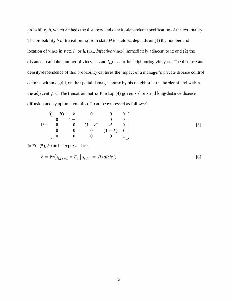
probability b, which embeds the distance- and density-dependent specification of the externality.

The probability b of transitioning from state H to state Eu depends on (1) the number and

location of vines in state 𝐼mor 𝐼h (i.e., Infective vines) immediately adjacent to it; and (2) the

distance to and the number of vines in state 𝐼mor 𝐼h in the neighboring vineyard. The distance and

density-dependence of this probability captures the impact of a manager’s private disease control

actions, within a grid, on the spatial damages borne by his neighbor at the border of and within

the adjacent grid. The transition matrix P in Eq. (4) governs short- and long-distance disease

diffusion and symptom evolution. It can be expressed as follows:4

P =

(1 − 𝑏) 𝑏 0 0 00 1 − 𝑐 𝑐 0 00 0 (1 − 𝑑) 𝑑 00 0 0 (1 − 𝑓) 𝑓0 0 0 0 1

[5]

In Eq. (5), 𝑏 can be expressed as:

𝑏 = Pr(𝑠𝑖,𝑗,𝑡+1 = 𝐸𝑢 | 𝑠𝑖,𝑗,𝑡 = 𝐻𝑒𝑎𝑙𝑡ℎ𝑦) [6]

13

=

{

1 − 𝑒−𝛾𝐿,𝐻,𝑗,𝑡 if 𝑠𝑁𝑖,𝑗,𝑡 = (𝑁𝐼, 𝑁𝐼, 𝑁𝐼, 𝑁𝐼)

1 − 𝑒−(𝛽+𝛾𝐿,𝐻,𝑗,𝑡) if 𝑠𝑁𝑖,𝑗,𝑡 = (𝑁𝐼, 𝑁𝐼, 𝐼, 𝑁𝐼)

1 − 𝑒−(𝛽+𝛾𝐿,𝐻,𝑗,𝑡) if 𝑠𝑁𝑖,𝑗,𝑡 = (𝑁𝐼, 𝑁𝐼, 𝑁𝐼, 𝐼)

1 − 𝑒−(2𝛽+𝛾𝐿,𝐻,𝑗,𝑡) if 𝑠𝑁𝑖,𝑗,𝑡 = (𝑁𝐼, 𝑁𝐼, 𝐼, 𝐼)

1 − 𝑒−(𝛼+𝛾𝐿,𝐻,𝑗,𝑡) if 𝑠𝑁𝑖,𝑗,𝑡 = (𝐼, 𝑁𝐼, 𝑁𝐼, 𝑁𝐼)

1 − 𝑒−(𝛼+𝛽+𝛾𝐿,𝐻,𝑗,𝑡) if 𝑠𝑁𝑖,𝑗,𝑡 = (𝐼, 𝑁𝐼, 𝐼, 𝑁𝐼)

1 − 𝑒−(𝛼+𝛽+𝛾𝐿,𝐻,𝑗,𝑡) if 𝑠𝑁𝑖,𝑗,𝑡 = (𝐼, 𝑁𝐼, 𝑁𝐼, 𝐼)

1 − 𝑒−(𝛼+2𝛽+𝛾𝐿,𝐻,𝑗,𝑡) if 𝑠𝑁𝑖,𝑗,𝑡 = (𝐼, 𝑁𝐼, 𝐼, 𝐼)

1 − 𝑒−(𝛼+𝛾𝐿,𝐻,𝑗,𝑡) if 𝑠𝑁𝑖,𝑗,𝑡 = (𝑁𝐼, 𝐼, 𝑁𝐼, 𝑁𝐼)

1 − 𝑒−(𝛼+𝛽+𝛾𝐿,𝐻,𝑗,𝑡) if 𝑠𝑁𝑖,𝑗,𝑡 = (𝑁𝐼, 𝐼, 𝐼, 𝑁𝐼)

1 − 𝑒−(𝛼+𝛽+𝛾𝐿,𝐻,𝑗,𝑡) if 𝑠𝑁𝑖,𝑗,𝑡 = (𝑁𝐼, 𝐼, 𝑁𝐼, 𝐼)

1 − 𝑒−(𝛼+2𝛽+𝛾𝐿,𝐻,𝑗,𝑡) if 𝑠𝑁𝑖,𝑗,𝑡 = (𝑁𝐼, 𝐼, 𝐼, 𝐼)

1 − 𝑒−(2𝛼+𝛾𝐿,𝐻,𝑗,𝑡) if 𝑠𝑁𝑖,𝑗,𝑡 = (𝐼, 𝐼, 𝑁𝐼, 𝑁𝐼)

1 − 𝑒−(2𝛼+𝛽+𝛾𝐿,𝐻,𝑗,𝑡) if 𝑠𝑁𝑖,𝑗,𝑡 = (𝐼, 𝐼, 𝐼, 𝑁𝐼)

1 − 𝑒−(2𝛼+𝛽+𝛾𝐿,𝐻,𝑗,𝑡) if 𝑠𝑁𝑖,𝑗,𝑡 = (𝐼, 𝐼, 𝑁𝐼, 𝐼)

1 − 𝑒−(2𝛼+2𝛽+𝛾𝐿,𝐻,𝑗,𝑡) if 𝑠𝑁𝑖,𝑗,𝑡 = (𝐼, 𝐼, 𝐼, 𝐼)

In Eq. (6), 𝑠N𝑖,𝑗,𝑡is the infectivity state of a vine’s neighborhood, which is composed of the

adjacent neighbors to the north, south, east, and west of vine (i, j). For example, 𝑠N𝑖,𝑗,𝑡= (I, I, I,

NI) is the state of a neighborhood composed of two Infective (I) north and south neighbors, one

Infective east neighbor and one Non-infective (NI) west neighbor. Cells on the edge of the grid

have only two or three neighbors. In these cases, as in the cases above, the exponential rate in

Eq. (6) has the 𝛾L,H,𝑗,𝑡 parameter, one 𝛼 parameter for each Infective neighbor in a north and

south position and a 𝛽 parameter for each Infective neighbor in an east or south position. For

example, the northwestmost cell has only two neighboring cells to the east and south and no

neighbors to the north and west. If both east and west neighbors are Infective in the positions,

𝑠N𝑖,𝑗,𝑡 = (𝑁𝐼, 𝐼, 𝐼, 𝑁𝐼) and 𝑏 = 1 − 𝑒−(𝛼+𝛽+𝛾𝐿,𝐻,𝑗,𝑡).

14

Short-Distance Diffusion

Parameters α and β are the within-column (north-south) and across-column (east-west)

transmission rates with α > β > 0.5 The period a vine stays in the Healthy state before

transitioning to the Exposed-undetectable state is an exponentially distributed random variable,

with rate α for within-column disease transmission and rate β for across-column disease

transmission. In each time step, a Healthy vine that has one within-column Infective neighbor

(e.g., 𝑠N𝑖,𝑗,𝑡 = 𝐼,𝑁𝐼, 𝑁𝐼, 𝑁𝐼) receives the infection at time t+1 if 𝑢𝑡 < 1 − 𝑒−𝛼 and does not

receive it if 𝑢𝑡 ≥ 1 − 𝑒−𝛼, where 𝑢𝑡 is a random draw from 𝑈~ (0, 1). Similarly, a Healthy vine

that has one across-column Infective neighbor (e.g., 𝑠𝑁𝑖,𝑗,𝑡 = 𝑁𝐼,𝑁𝐼, 𝐼, 𝑁𝐼) receives the infection

at time t+1 if 𝑢𝑡 < 1 − 𝑒−𝛽 and does not receive it if 𝑢𝑡 ≥ 1 − 𝑒−𝛽.). When two or more

transmission types are realized (e.g., one within- and two across-column events), the disease

transmission is determined by the shortest of the waiting times (Cox 1959).

Long-Distance Diffusion

Long-distance, vector-mediated disease diffusion from low-valued vineyard GL to its high-

valued counterpart GH occurs with rate 𝛾L,H,𝑗,𝑡. Here, 𝛾L,H,𝑗,𝑡 is a power-law dispersal parameter

specified by the following spatial-dynamic, distance- and density-dependent diffusion function.

In order to calculate the total number of infective vines in each period, we introduce indicator

variables 𝑥 and 𝑦 equaling 1 if a vine in column 𝑛 and row 𝑚 is Infective and 0 otherwise. If 𝑥 =

1, the corresponding vineyard rows that have 𝑦 = 1 contain infective vines (i.e., in state 𝐼mor 𝐼h)

that contribute to the long-distance diffusion from GL to GH. If 𝑥 = 0 for all columns 𝑛 (i.e.,

there are no infective vines in vineyard GL), the denominator equals 0, 𝛾L,H,𝑗,𝑡 is not defined, and

there is no long-distance diffusion from GL to GH.

𝛾L,H,𝑗,𝑡 = 𝑗− 𝛾 ∑ 𝑥∑ 𝑦((𝑥,𝑦)| 𝑠𝑚,𝑛,𝑡 = { 𝐼m,𝐼h})∗𝑥

𝑀𝑚

𝑁𝑛

∑ 𝑥 𝑀(𝑁−𝑥+1)𝑁𝑛

, 𝛾 > 0,∑ 𝑥 𝑀(𝑁 − 𝑥 + 1)𝑁𝑛 > 0 [7a]

15

Similarly, long-distance dispersal from GH to GL is given by:

𝛾H,L,𝑛,𝑡 = (𝑁 − 𝑛)− 𝛾

∑ 𝑥∑ 𝑦((𝑥,𝑦)| 𝑠𝑖,𝑗,𝑡= { 𝐼m,𝐼h})∗𝑦𝐽𝑗

𝐼𝑖

∑ 𝑦 𝐼(𝐽−𝑦+1)𝐽𝑗

, 𝛾 > 0,∑ 𝑦 𝐼(𝐽 − 𝑦 + 1)𝐽𝑗 > 0 [7b]

In Eq. (7a), for any vine (i, j), 𝛾L,H,𝑗,𝑡 is inversely proportional to the distance from the shared

boundary (i.e., distance from column j in GH to column 𝑁 in GL, regardless of its row position in

column j).6 We choose a power-law specification because it allows the disease long-distance

diffusion to have new infection foci emerging beyond the disease invading front, which is

consistent with modeling the wind dispersal of insects (Gibson 1997; Marco, Montemurro, and

Cannas 2011). Parameter 𝛾L,H,𝑗,𝑡 is also proportional to the total number of Infective vines in GL,

weighted by their column position n (the numerator in Eq. 7a). Weighting each Infective vine by

its column position n allows vines closer to the bordering column to contribute more to the

externality than vines situated farther from the boundary (i.e., cell-level distance dependence).

The denominator in Eq. (7a) allows the multiplier of the power-law expression to vary between 0

and 1 as the number of Infective vines in GL varies between 0 and M*N (i.e., density

dependence). In the baseline case, we initialize the disease in GL and the disease spreads to GH

according to Eq. (7a). Once vines in vineyard GH become Infective, they can act as a source of

infection for Healthy vines in vineyard GL according to Eq. (7b), thus making the externality

bidirectional.7 Note that this power-law specification allows local management and dispersal to

take place at different spatial scales, a modeling challenge identified by recent bioeconomic

studies (Aadland, Sims, and Finnoff 2015). This specification of dispersal is novel in that it

allows private actions of one manager in one management unit (i.e., the cell) to have

repercussions not only on neighboring units but also on non-neighboring units that are managed

by a different manager. Combined with short-distance dispersal, this distance and density

dependent specification of long-distance dispersal allows testing whether within-parcel spatial

16

considerations are also important for generating externalities. This is in contrast to extant

resource and environmental economics literature, which assumes that spatial considerations only

matter in that they define the spatial limit to private actions, and that managers ignore how their

management in one cell affects payoffs through multi-cell dispersal. For descriptions of

probabilities c, d, and f, we refer the reader to Atallah et al. (2015). Short- and long-distance

disease diffusion parameters are presented in Table 1 and Figure 1.

[Insert Table 1here]

IV. COMPUTATIONAL EXPERIMENTS AND SOLUTION FRAMEWORKS

We conducted Monte Carlo experiments, each consisting of a set of 1,000 simulations.

Experiments differ based on the strategy pairs employed in both vineyards to control the disease.

Outcome realizations for a given run within an experiment differ due to the random location of

initially infected vines in the grid where the disease is initialized (GL, for the baseline case), and

stochastic disease diffusion within and between vineyards. Data collected over simulation runs

are the NPV realizations under each strategy pair.

Model Initialization

Grapevines are initialized as Healthy and of age equal to zero in both vineyards GH and GL

(high- and low-valued vineyard, respectively). At t=1, seven percent of the grapevines in GL are

chosen at random from U (0, M*N) to transition from state Healthy to state Exposed-

undetectable.8 Subsequently, the disease spreads to Healthy vines within GL according to the

Markov transition process given by Eq. (4) and Eq. (5). The Infective vines in GL act as a

primary source of long-distance disease diffusion to the Healthy vines in GH. The disease spreads

from GL to GH according to the distance- and density-dependent diffusion function 𝛾L,H,𝑗,𝑡 (Eq.

17

7a). Subsequently, Infective vines in GH act as a source of reinfection in GL according to the

distance- and density-dependent diffusion function 𝛾H,L,𝑛,𝑡 (Eq. 7b) and so on. Economic

parameters are presented in Table 2.

[Insert Table 2 here]

Nonspatial, Spatial, and Fire-Break Strategies

Nonspatial strategies (strategies 1 to 8, Table 3) consist of removing and replacing vines based

on symptoms alone (Infective-moderate; Infective-high) or based on symptoms and age of

individual vines (Young: 0-5 years; Mature: 6-19 years; Old: 20 years and above).9 In the subset

of spatial strategies (strategies 9 to 18, Table 3), the manager removes and replants symptomatic

vines (Infective-moderate) and tests their neighbors. Neighboring vines are removed and

replaced if they test positive. In that sense, the manager's spatial disease control decisions are

based on a vine’s own state and the state of vines in neighboring cells. For example, according to

strategy ImNS (Table 3), vines in cells (i-1, j) and (i+1; j) would be removed and replaced based

on the state of vine in cell (i,j); according to strategy ImNSEW, vines in cells (i-1, j), (i+1; j), (i, j-

1) and (i, j+1) would be removed and replaced based on the state of vine in cell (i,j), and

similarly for all within-grid, spatial strategies. The third subset of strategies includes fire-break

strategies that consist of removing (without replanting) vines in the border columns of a vineyard

in order to create ‘fire-breaks’ or ‘buffer zones’ that would reduce long-distance disease

diffusion between vineyards through the distance- and density-dependence in Equations (7a) and

(7b) (Strategy 19 to Strategy 57 in Table 3). Fire-break strategies are intended to decrease the

effect of spillovers between vineyards and can give a manager control over their disease risk. All

strategies are available to both managers. Note that we do not consider vector management

strategies, which can be ineffective when vectors can spread disease rapidly even if their

18

population is kept at a low density (Charles et. al 2009; Tsai et al. 2008). Control of such insect-

transmitted plant diseases relies mostly on reducing the source of infection by removing infected

plants and replacing them with young, healthy ones (Chan and Jeger 1994).


Solution Frameworks and Game Theoretic Solution Concepts

We employ the objective function (Eq. 3) to rank the vineyard ENPVs under the alternative

disease control strategy pairs. We first solve the social planner problem and cooperative solution

(C). The solution to these problems is relevant for situations where one vineyard management

firm manages contiguous vineyards that produce wine grapes of different qualities. Second, we

solve for the noncooperative solution (NC). Third, whenever the cooperative surplus is strictly

positive, we find the cooperative solution that satisfies the Nash bargaining framework.

Social Planner

The social planner chooses the pair of disease management strategies (𝒲H ,𝒲L) that maximizes

the total payoff (ENPVT), the sum of the expected net present values of GL (ENPVL) and GH

(ENPVH). The following maximization problem is solved:

𝑚𝑎𝑥(𝒲H ,𝒲L)

𝐸𝑁𝑃𝑉H + 𝐸𝑁𝑃𝑉L, [8a]

subject to:

𝐸(𝒔𝑖,𝑗,𝑡+1) = 𝐏𝑇 𝒔𝑖,𝑗,𝑡, [8b]

and

𝐸(𝒔𝑚,𝑛,𝑡+1) = 𝐏𝑇 𝒔𝑚,𝑛,𝑡 [8c]

where Eq. (8b) and Eq. (8c) are the cell-level infection state transition equations in GH and GL,

respectively.

19

Noncooperative Disease Control

We use the Nash equilibrium solution concept to solve a simultaneous-move game where the

managers do not cooperate and do not share any information about their strategies. We use the

subgame perfect Nash equilibrium concept to solve a sequential game with asymmetry of

information where one player moves first and the other player makes his choice accordingly

(Tirole, 1988). In both simultaneous and sequential move cases, we consider situations where the

disease starts in GL and in GH. Note that the managers do not face a common or shared state

variable: each manager contends with the stochastic evolution of the disease in his vineyard (Eq.

8b and 8c) while not knowing the status of the disease in the neighboring vineyard. They only

observe the control strategy being adopted by the neighboring manager (expect for the

simultaneous-move case).

Cooperative Disease Control: Nash Bargaining Game

To solve the cooperative disease control game, we use the static axiomatic approach, specifically

the Nash bargaining game (Nash 1953; Binmore, Rubinstein, and Wolinsky 1986). The Nash

bargaining game here is similar to the one used in Munro (1979) to solve for the payoffs in a

static, cooperative game with side payments and fixed disagreement payoffs. The relationship

between the two players, as described by Nash (1953), interpreted by Luce and Raiffa (1967, p.

138), and applied in Munro (1979) and others, consists of the players entering into a binding

agreement at the beginning of the game whereby each receives the return they would expect

without an agreement and half of the cooperative surplus. If the two vineyards are cooperatively

managed, the two managers solve the Nash bargaining game, the solution to which is the unique

pair of cooperative payoffs (𝐸𝑁𝑃𝑉H𝐶 , 𝐸𝑁𝑃𝑉L

C) that solves the following maximization problem

(Nash 1953; Munro 1979; Sumaila 1997):

20

𝑚𝑎𝑥{𝐸𝑁𝑃𝑉H, 𝐸𝑁𝑃𝑉L}

(𝐸𝑁𝑃𝑉HC − 𝐸𝑁𝑃𝑉H

NC) (𝐸𝑁𝑃𝑉LC − 𝐸𝑁𝑃𝑉L

NC), [9]

subject to:

𝐸𝑁𝑃𝑉C ≥ 𝐸𝑁𝑃𝑉NC, [10]

and subject to the disease diffusion functions in GH (Eq. 8b) and GL (Eq. 8c). The maximand in

Eq. (9), known as the Nash product, is the product of the differences between the cooperative

and noncooperative payoffs from GH and GL, and inequality (10) is the incentive compatibility

constraint. Under the standard axioms of bargaining theory, Eq. (9) has the following unique

solution (Muthoo 1999):10

𝐸𝑁𝑃𝑉HC = 𝐸𝑁𝑃𝑉H

NC +1

2 (𝐸𝑁𝑃𝑉T

C − 𝐸𝑁𝑃𝑉TNC) [11]

𝐸𝑁𝑃𝑉LC = 𝐸𝑁𝑃𝑉L

NC + 1

2 (𝐸𝑁𝑃𝑉T

C − 𝐸𝑁𝑃𝑉TNC) [12]

In the solution described by Eq. (11) and Eq. (12), 𝐸𝑁𝑃𝑉HNCand 𝐸𝑁𝑃𝑉L

NC are the expected

noncooperative payoffs (i.e., the disagreement points) for GH and GL, respectively and

(𝐸𝑁𝑃𝑉TC − 𝐸𝑁𝑃𝑉T

NC) is the expected cooperative surplus. The expected cooperative surplus is

defined as the difference between the total expected cooperative payoff (𝐸𝑁𝑃𝑉TC = 𝐸𝑁𝑃𝑉H

C +

𝐸𝑁𝑃𝑉LC) and the total expected noncooperative payoff (𝐸𝑁𝑃𝑉T

NC = 𝐸𝑁𝑃𝑉HNC + 𝐸𝑁𝑃𝑉L

NC). The

expected cooperative surplus is also a measure of the Pareto-inefficiency caused by

noncooperative disease control.11

21

V. EXTERNALITY CONTROL, HETEROGENEITY AND STRATEGIC

BEHAVIOR

Social Planner and Cooperative Control

If the vineyards are managed by a single entity or a social planner, the total payoff is highest

($122,000/acre) when the disease is managed in both vineyards under strategy ImNS, which

targets symptomatic vines and their two within-column neighbors (Table 4). If the vineyards are

individually managed and the managers agree to cooperatively control the disease, the Nash

bargaining solution consists of (ImNS, ImNS) with payoffs (80, 42) after the managers equally

share the cooperative surplus according to Eq. (11) and Eq. (12) (Table 4).


Noncooperative Control

In a simultaneous game, we find a unique Nash equilibrium pair of strategies that consists of

no control in either vineyard, with payoffs (60, 22) for the managers of the high, and low-valued

vineyards, respectively (Table 4; see Table A1 in the appendix for the payoff matrix). In a

sequential game where the low-valued vineyard moves first, (no control, no control) is the

subgame perfect Nash equilibrium. The payoffs from the solution to the Nash bargaining

problem indicate that, if the two vineyard managers cooperate and agree to implement spatial

Strategy ImNS in their respective vineyards, there is a cooperative surplus of $40,000 for the two

acres. This surplus is statistically different from zero at the 1% level (as determined by the

variation in the Monte Carlo replications) and represents a welfare (ENPVT) gain of

approximately 47% over the noncooperative outcome. These benefits to cooperation are

consistent with previous findings from studies on the cooperative management of fisheries

(Sumaila 1997) and nuisance wildlife species (Bhat and Huffaker 2007).

22

Interestingly, we find that the social planner solution can be achieved, without cooperation,

when the high-value manager moves first. In that case, his optimal strategy is spatial control

ImNS. Given GH’s commitment to spatially control the disease, GL’s value of control increases

due to the strategic complement nature of disease (or pest) control with neighbor-to-neighbor

spillovers (Fenichel, Richards, and Shanafelt 2014). GL’s optimal strategy is spatial control,

ImNS, as well, with payoff $31,000/acre. The strategic complement nature of transboundary

disease control also explains why (no control, no control) is the subgame perfect Nash

equilibrium strategy in a sequential game where GL moves first as well as in a simultaneous

game.

Welfare Effects of the Externality Specification

We measure the welfare implications of including the detailed within-parcel, spatial,

biophysical process in our specification of the externality and its control. We do so by

comparing the model’s outcomes to those obtained from management decisions using strategies

that ignore the within-parcel spatial dynamics of the biophysical process. We restrict the set of

disease control strategies to those that are nonspatial and those that consist of ‘fire-breaks’

(strategies 1 through 8, and 19 through 57, respectively, in Table 3). We solve the problem to

rank these strategies under the social planner, the cooperative, and the noncooperative

simultaneous game settings. Including the within-parcel spatial dynamics leads to strategy (ImNS,

ImNS), with total payoffs of $122,000. A model that ignores a manager’s ability to make within-

parcel decisions leads to the strategy pair (no control, no control) with lower payoffs totaling

$82,000. This suggests that ignoring the within-parcel spatial dynamics underestimates the

payoffs and overestimates the social cost of the externality. 12

23

In order to isolate the effect of within-parcel spatial dynamics from the effect of virus testing,

we consider an additional strategy whereby a manager removes and replaces grapevines that are

symptomatic, conducts spatially random virus tests (based on the number that would have been

obtained under the spatial strategy ImNS), and removes and replants the grapevines that test

positive. We find that random testing leads to total payoffs that are lower than those obtained

under no control. If both managers adopt random testing, total payoffs are $55,000, which is

34% lower than strategy pair (no control, no control). This strategy pair still leads to the

maximum total payoffs if within-parcel spatial dynamics are ignored, even if non-spatial testing

is considered.

Sensitivity Analysis

We conduct a sensitivity analysis to examine the effect of changes in the values of key within-

parcel and across-parcel disease diffusion parameters on the externality’s welfare impacts. These

parameters are the short-distance parameter 𝛼 in Eq. 6; the long-distance diffusion parameter 𝛾 in

Eq. (7a) and Eq. (7b); the vineyard size parameters I, J, M, and N in these same equations; and

disease initialization.

First, we find that reducing the value of the short-distance parameter 𝛼 by half (from 4.2 to

2.1) causes aggregate welfare to increase by 52% in a noncooperative, simultaneous game or in a

noncooperative, sequential game where GL moves first. In such games, GL controls the disease

and therefore the externality, in which case GH does not control. The increase in welfare is

(expectedly) more modest (3%) in game settings leading to both managers spatially controlling

the disease (the noncooperative game where GH moves first and Nash bargaining game). (Percent

changes are obtained by comparing payoffs in Table 5 with those in Table A2 of the appendix).

Reduction in the value of the short-distance parameter can be achieved by increasing the distance

24

between grapevines within the grid’s columns and suggests that individual, within-parcel choices

about the physical configuration of the vineyard can directly impact the welfare effects of an

externality.

Second, we solve the baseline problem for larger and smaller values of the long-distance

transmission coefficient 𝛾. 13 For a larger long-distance transmission coefficient (i.e., where

disease transmission is characterized by a more rapid decline over space and the vineyards are

therefore less ecologically connected), the manager of the lower-value vineyard spatially controls

the disease, in which case the GH does not need to control (Table A3-a of the appendix). The

outcome (no control, ImNS) does not depend on the type of game played. If the long-distance

transmission coefficient has a smaller value than in the baseline case, none of the managers

control the disease in any of the noncooperative game solutions and the strategy pair (ImNS, Exit)

is the central planner’s solution (Table A3-b of the appendix). These results identify an upper

bound for the long-distance diffusion coefficient where the externality does not trigger any

control in the neighboring vineyard and a lower bound where the externality is large enough to

warrant removal of the lower-valued vineyard by a central planner. Changes in the value of 𝛾 can

be achieved by modifying the biophysical environment that affects the extent to which the

vineyards are ecologically connected, such as physical barriers or other pest management

practices that reduce the flow of insect vectors.

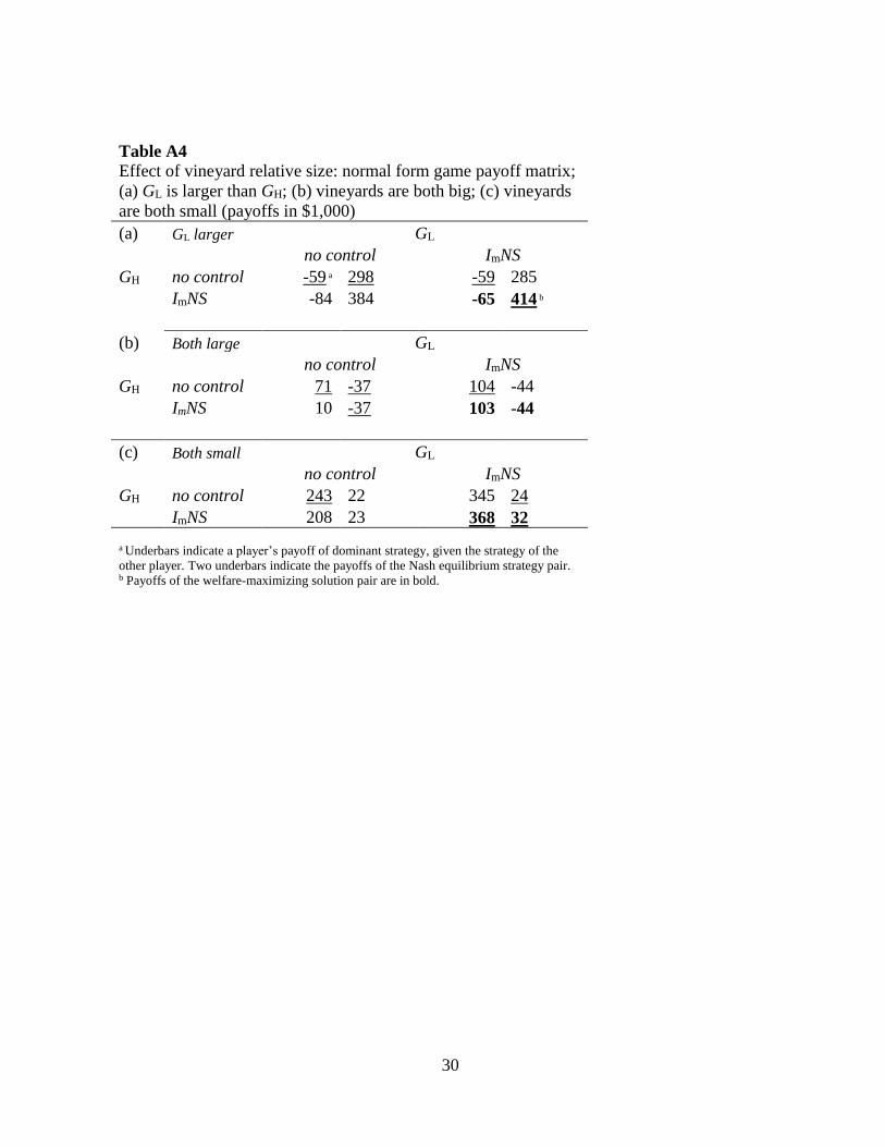
Third, we explore the effect of the relative vineyard size. Recall that in the baseline case, GH

is larger than GL, the NE strategy pair is (no control, no control), and the noncooperative payoffs

are 32% lower than the cooperative or social planner payoffs, generated by the strategy pair

(ImNS, ImNS). If the relative size of the vineyards is reversed (GL larger than GH) or if both

vineyards are large, we obtain the same strategy pair solutions. The noncooperative,

25

simultaneous game’s total payoffs are 31 and 41% lower than the cooperative payoffs, if GL is

larger or both are large, respectively (Table A4-a and A4-b). However, if both vineyards are

smaller, strategy (ImNS, ImNS) is the strategy pair solution in all frameworks and the externality

is minimized (Table A4- c). The results from the vineyard size scenario analysis are driven by

disease population dynamics: a larger vineyard has a larger population of Susceptible grapevines,

which speeds disease diffusion and renders disease control less effective (and less cost-effective)

than a strategy of no control.

Fourth, we explore the implications of the disease beginning in the high-valued vineyard, as

opposed to the most likely case where the disease starts in the low-valued vineyard. Initializing

the disease in GH instead of GL leads to the Nash equilibrium (ImNS, ImNS) no matter whether the

game is simultaneous or sequential, noncooperative or cooperative (Table A5 of the appendix).

In the baseline case, an uncontrolled lower-valued vineyard provides a reserve for the disease,

affects the incentives for control in GH, and leads to the Nash equilibrium (no control, no

control).

Heterogeneity, Strategic Behavior, and Total Payoff

We now turn to addressing whether and how resource value heterogeneity affects strategic

disease control decisions and total payoffs. We solve the problem for four additional price pairs:

starting with the baseline price pair (Table 5, case 5), we consider four mean-preserving price

contractions (Table 5, cases 1 to 4) to cover the distribution of prices that are observed for

Cabernet franc in the Napa County Grape Pricing District (CDFA 2014). 14 For consistency, we

also change the quality penalties linearly with price changes across cases (Table 5). Results in

Table 5 show that the difference in prices and penalties faced by the managers of GH and GL has

a substantial impact on the managers’ aggregate payoffs and on their strategic behavior in

26

disease control. The quality penalty is greater for higher-valued grapes, which causes disease

damages to increase and welfare to decrease as we move from case 1 to case 5. In cases 1

through 4, both managers choose Strategy ImNS regardless of whether the game is simultaneous

or sequential, cooperative or noncooperative. In these cases, prices received for grapes in both

vineyards are high enough for the managers to afford Strategy ImNS. Still, even though both

managers spatially control, because an increasingly larger penalty being applied to the higher

price as we move from case 1 to case 4, aggregate damages increase and aggregate welfare

decreases.


In case 5, heterogeneity affects aggregate payoffs not only through the interaction effect of

prices and penalties (as in cases 1 to 4) but also through its effect on the strategic behavior of

managers. In case 5, due to the different prices and penalties they face, GL opts for no control

when he moves first while GH opts for ImNS when he moves first. The second mover chooses the

same strategy as the first mover and the unique subgame perfect Nash equilibrium is, therefore,

(no control, no control) if GL moves first and (ImNS, ImNS) if GH moves first. This result can be

explained by the weaker-link public good nature of disease control provision where the action of

one agent either increases or decreases the returns to control for the other agent, suggesting that

decisions are strategic complements (Cornes 1993; Fenichel, Richards, and Shanafelt 2014). It is

this strategic complementarity in the provision of disease control that causes the first move in GH

to change the payoff space for the second mover and increase the value of disease control in GL,

thereby replicating the public planner result. One implication of this model is that the extent to

which the pubic good is underprovided is systematically related to the degree of heterogeneity

among agents (Cornes 1993; Fenichel, Richards, and Shanafelt 2014).

27

Along the various degrees of heterogeneity represented in the five noncooperative setting

cases (cases 1 through 5, simultaneous and sequential settings), total payoff is monotonically

decreasing in the level of heterogeneity (i.e., the magnitude of price gap).15 In a cooperative

game, the drop in total payoffs between cases 4 and 5 is less pronounced due to Nash bargaining

in case 5. Figure 2 shows that heterogeneity in resource value substantially reduces welfare and

that at extreme resource value heterogeneity levels, cooperative control attenuates that impact in

comparison to noncooperative control.

[Insert Figure 2 here]

VI. CONCLUSIONS

In this paper, we examined how metapopulation models and cellular automata can be

combined to develop a novel distance- and density-dependent specification of externalities that

acknowledges the importance of inter- and within-parcel spatial dynamics in the generation and

control of externalities. Our specification is general in that it can be collapsed to represent

metapopulation models only, cellular automata models only, or a combination of the two, with

short-distance diffusion only, long-distance diffusion only, or with both, depending on the

characteristics of the process generating the externalities.

We used this specification to solve spatial noncooperative and cooperative games that

endogenize spatial risk beyond the immediate neighborhood and capture the inter- and within-

parcel private incentives to control. We found that within-parcel spatial decisions can generate

the externality and may lead to inefficient outcomes in the decentralized management of public

bads. We also showed that noncooperative strategic spatial decisions within the parcel can lead

to efficient outcomes even in the absence of Coasian bargaining (Coase 1960). Finally, we have

28

characterized the relationship among resource value heterogeneity, strategic behavior, and total

payoffs. Our analysis, with heterogeneity, allows of different, first-move-dependent,

noncooperative equilibria ranging from no control to spatial control to entire vineyard removal.

Our work contributes to the growing literature that examines the spatial-dynamic nature of

externalities by increasing the spatial dimension of the problem and the number of players

making strategic decisions. We show that increased computational power that has allowed

researchers to consider larger grids and a greater number of players, can also be used to

understand the spatial dynamics within a parcel that determine the generation of externalities and

private incentives to control. Our results suggest that ignoring the complex biophysical details of

the within-parcel spatial dynamics can lead to misleading measures of welfare impacts of

externalities.

Our model makes valuable contributions to the literature that can be extended to examine

other types of spatial-dynamic externalities. Yet, it has several limitations that should be

addressed in future research. For instance, the model does not offer clear insights into the

cooperative management of externalities in which disagreement payoffs (i.e., noncooperative

payoffs) are not fixed, agreement renegotiation is needed and there are more than two players. In

such situations, differential games with N players might be appropriate but solution methods for

such games require restrictive assumptions about the state equations and game solutions are not

guaranteed (Bressan 2011). In parallel to the on-going research on whether stable solutions exist,

future research might use learning dynamics to explore whether solutions to spatial-dynamic

externalities in N-player bargaining games are achievable (Smead et al. 2014). Such effort might

identify reasons why desirable solutions might not be attainable and the mechanisms that might

be implemented to increase the likelihood of reaching these solutions.

29

APPENDIX

Table A1

Normal form game payoff matrix for the baseline case (payoffs in $1,000)

GL

no control a ImY ImNS

GH

no control 60 b 22 81 -11 98 -5

ImY 41 1 81 -11 93 -5

ImNS

-20

1

25

-11

91

31

a Underbars indicate a player’s payoff of dominant strategy, given the strategy of the other player. b Payoffs of the welfare-maximizing solution pair are in bold.

Table A2

Effect of a smaller short-distance diffusion parameter (α=2.1): normal

form game payoff matrix (payoffs in $1,000)

GL

no control ImNS

GH no control 60 23 98 27

ImNS

-14

23

93

32


Table A3

Effect of (a) larger (γ=3.5) and (b) smaller (γ=1.5) long-distance diffusion

parameter: normal form game payoff matrix (payoffs in $1,000).

(a) γ=3.5 GL

no control ImNS Exit

no control 78 a 23 103 29 b 93 -5

GH ImNS 12 23 95 31 110 -5

Exit -11 23 -11 31 -11 -5

(b) γ=1.5 GL


no control -13 19 34 -77 52 -5

GH ImNS -316 21 13 14 94 -5

Exit -11 23 -11 30 -11 -5

a Underbars indicate a player’s payoff of dominant strategy, given the strategy of the other player. Two underbars indicate the

payoffs of the Nash equilibrium strategy pair. b Payoffs of the welfare-maximizing solution pair are in bold.

30

Table A4

Effect of vineyard relative size: normal form game payoff matrix;

(a) GL is larger than GH; (b) vineyards are both big; (c) vineyards

are both small (payoffs in $1,000)

(a) GL larger GL

no control ImNS

GH no control -59 a 298 -59 285

ImNS -84 384 -65 414 b

(b) Both large GL

no control ImNS

GH no control 71 -37 104 -44

ImNS 10 -37 103 -44

(c) Both small GL

no control ImNS


ImNS 208 23 368 32

a Underbars indicate a player’s payoff of dominant strategy, given the strategy of the

other player. Two underbars indicate the payoffs of the Nash equilibrium strategy pair. b Payoffs of the welfare-maximizing solution pair are in bold.

31

Table A5 Expected payoffs under the social planner, noncooperative, and cooperative solutions, case where disease starts in GH

Setting Solution strategy pairs Expected Payoffs a

𝐺H, 𝐺L 𝐸𝑁𝑃𝑉H; 𝐸𝑁𝑃𝑉L 𝐸𝑁𝑃𝑉T

Simultaneous ImNS, ImNS 5, 76 81

Sequential-GL moves first ImNS, ImNS 5, 76 81

Sequential-GH moves first ImNS, ImNS 5, 76 81 a Expectations are obtained from 1,000 simulations over 50 years; payoffs are in $1,000/acre and are

computed for the baseline prices pH=$5,058/ton and pL=$726/ton.

32

Acknowledgements

Atallah acknowledges support from the Cornell Land-Grant Fellowship. The authors are grateful

to Janus Thorsten, Ravi Kanbur, and anonymous reviewers for comments. Any errors are solely

the authors’.

33

References

Aadland, D., C. Sims, and D. Finnoff. 2015. “Spatial Dynamics of Optimal Management in

Bioeconomic Systems.” Computational Economics 45 (4): 544-577.

Albers, H.J., C. Fischer, and J.N. Sanchirico. 2010. “Invasive species management in a spatially

heterogeneous world: Effects of uniform policies.” Resource and Energy Economics 32 (4): 483-

499.

Atallah, S. S., M. I. Gómez, J. M. Conrad and J. P. Nyrop. 2015. “A Plant-Level, Spatial,

Bioeconomic Model of Plant Disease Diffusion and Control: Grapevine Leafroll Disease.”

American Journal of Agricultural Economics 97 (1): 199–218.

Binmore, K., A. Rubinstein, and A. Wolinsky. 1986. “The Nash bargaining solution in economic

modelling.” The RAND Journal of Economics 176-188.

Bhat M. G. and R. G. Huffaker. 2007. “Management of a transboundary wildlife population: A

self-enforcing cooperative agreement with renegotiation and variable transfer payments.”

Journal of Environmental Economics and Management 53 (1): 54-67.

Bressan, A. 2011. “Non-cooperative Differential Games.” Milan Journal of Mathematics 79 (2):

357-427.

Brown, C., L. Lynch, and D. Zilberman. 2002. “The economics of controlling insect-transmitted

plant diseases.” American Journal of Agricultural Economics 84 (2): 279-291.

Brown, G., and J. Roughgarden. 1997. “A metapopulation model with private property and a

common pool.” Ecological Economics 22 (1): 65-71.

Cabaleiro, C., C. Couceiro, S. Pereira, M. Cid, M. Barrasa and A. Segura. 2008. “Spatial analysis

of epidemics of Grapevine leafroll associated virus-3.” European Journal of Plant Pathology

34

121 (2): 121-130.

Cabaleiro, C., and A. Segura. 1997. “Field transmission of grapevine leafroll associated virus 3

(GLRaV-3) by the mealybug Planococcus citri.” Plant Disease 81 (3): 283-287.

Cabaleiro, C., and A. Segura. 2006. “Temporal analysis of grapevine leafroll associated virus 3

epidemics.” European Journal of Plant Pathology 114 (4) 441-446.

Coase, R. H. 1960. “The problem of social cost.” In Classic Papers in Natural Resource

Economics, 87-137. Palgrave Macmillan UK.

California Department of Food and Agriculture. 2014. California Grape Crush Report 2013.

Available at

https://www.nass.usda.gov/Statistics_by_State/California/Publications/Grape_Crush/Final/2013/

201303gcbtb00.pdf. (accessed November 17, 2014).

Chan, M.S., and M.J. Jeger. 1994. “An analytical model of plant virus disease dynamics with

roguing and replanting.” Journal of Applied Ecology 31 (3): 413-427.

Charles, J. G., K. J. Froud, R. van den Brink, and D. J. Allan. 2009. “Mealybugs and the spread

of grapevine leafroll-associated virus 3 (GLRaV-3) in a New Zealand vineyard.” Australasian

Plant Pathology 38 (6): 576-583.

Cooper, M. L., K. Klonsky, and R. L. De Moura. 2012. Sample Costs to Establish a Vineyard

and Produce Winegrapes: Cabernet Sauvignon in Napa County. University of California

Cooperative Extension. Available at http://coststudies.ucdavis.edu/files/WinegrapeNC2012.pdf

(accessed November 17, 2014).

Cornes, R. 1993. “Dyke maintenance and other stories: Some neglected types of public

goods.” The Quarterly Journal of Economics 108 (1): 259-271.

Cox, D. R. 1959. “The analysis of exponentially distributed life-times with two types of failure.”

35

Journal of the Royal Statistical Society. Series B (Methodological) 411-421.

Epanchin-Niell, R. S., and J. E. Wilen. 2012. “Optimal spatial control of biological

invasions.” Journal of Environmental Economics and Management 63 (2): 260-270.

Epanchin-Niell, R. S., and J. E. Wilen. 2015. “Individual and Cooperative Management of

Invasive Species in Human-mediated Landscapes.” American Journal of Agricultural Economics

97 (1): 180-198.

Fenichel, E. P., T. J. Richards, and D. W. Shanafelt. 2014. “The control of invasive species on

private property with neighbor-to-neighbor spillovers.” Environmental and Resource Economics

59 (2): 231-255.

Gibson, G. J. 1997. “Markov chain Monte Carlo methods for fitting spatiotemporal stochastic

models in plant epidemiology.” Journal of the Royal Statistical Society: Series C (Applied

Statistics) 46: 215-233.

Grasswitz, T. R., and D. G. James. 2008. “Movement of grape mealybug, Pseudococcus maritimus,

on and between host plants.” Entomologia Experimentalis et Applicata 129 (3): 268-275.

Horan, R.D., C.A. Wolf, E.P. Fenichel, and K.H Matthews. 2005. “Spatial Management of

Wildlife Disease.” Review of Agricultural Economics 27 (3): 483-490.

Klonsky K. and P. Livingston. 2009. Cabernet Sauvignon Vine Loss Calculator. University of

California, Davis. Available at http://coststudies.ucdavis.edu/tree_vine_loss/ (accessed

November 17, 2014).

Konoshima, M., C. A. Montgomery, H. J. Albers, and J. L. Arthur. 2008. “Spatial-endogenous

fire risk and efficient fuel management and timber harvest.” Land Economics 84(3): 449-468.

Kovacs, K.F., R.G., Haight, R.J., Mercader, and D.G., McCullough. 2014. “A bioeconomic

analysis of an emerald ash borer invasion of an urban forest with multiple jurisdictions.” Resource

36

and Energy Economics 36 (1): 270-289.

Le Maguet, J., J.-J. Fuchs, J. Chadœuf, M. Beuve, E. Herrbach and O. Lemaire. 2013. “The role

of the mealybug Phenacoccus aceris in the spread of Grapevine leafroll-associated virus− 1

(GLRaV-1) in two French vineyards.” European Journal of Plant Pathology 135 (2): 415-427.

Luce, R. D. and H. Raiffa. 1967. Games and Decisions. Wiley, New York.

Marco, D.E., M. A. Montemurro, and S. A. Cannas. 2011. “Comparing short and long‐distance

dispersal: modelling and field case studies.” Ecography 34 (4): 671-682.

Munro, G. R. 1979. “The optimal management of transboundary renewable

resources.” Canadian Journal of Economics 12: 355-376.

Muthoo, A. 1999. Bargaining theory with applications. Cambridge University Press.

Nash, J. 1953. “Two-person cooperative games.” Econometrica: Journal of the Econometric

Society: 128-140.

Rich, K. M., A. Winter-Nelson, and N. Brozović. 2005a. “Regionalization and Foot-and-Mouth

Disease Control in South America: Lessons from Spatial Models of Coordination and

Interactions.” The Quarterly Review of Economics and Finance 45 (2): 526-540.

Rich, K. M., A. Winter-Nelson, and N. Brozović. 2005b. “Modeling Regional Externalities with

Heterogeneous Incentives and Fixed Boundaries: Applications to Foot and Mouth Disease Control

in South America.” Review of Agricultural Economics 27 (3): 456-464.

Sanchirico, J.N. and J.E. Wilen. 1999. “Bioeconomics of Spatial Exploitation in a Patchy

Environment.” Journal of Environmental Economics and Management 37 (2): 129-150.

Sims, C., D. Aadland and D. Finnoff. 2010. “A dynamic bioeconomic analysis of mountain pine

beetle epidemics.” Journal of Economic Dynamics & Control 34 (12): 2407-2419.

Smead, R., R. L. Sandler, P. Forber, and J. Basl. 2014. “A bargaining game analysis of

37

international climate negotiations.” Nature Climate Change 4 (6): 442-445.

Smith, M. D., J. N. Sanchirico, and J. E. Wilen. 2009. “The economics of spatial-dynamic

processes: applications to renewable resources.” Journal of Environmental Economics and

Management 57 (1): 104-121.

Sumaila, U. R. 1997. “Cooperative and non-cooperative exploitation of the Arcto-Norwegian

cod stock.” Environmental and Resource Economics 10 (2): 147-165.

Swallow, S.K., and D.N. Wear. 1993. “Spatial Interactions in Multiple-Use Forestry and

Substitution and Wealth Effects for the Single Stand.” Journal of Environmental Economics and

Management 25 (2): 103-120.

Tirole, J. 1988. The theory of industrial organization. MIT press.

Tsai, C.W., A. Rowhani, D.A. Golino, K.M. Daane, and R.P.P. Almeida. 2010. “Mealybug

Transmission of Grapevine Leafroll Viruses: an Analysis of Virus-Vector Specificity.”

Phytopathology 100 (8): 830-834.

Tsai, C-W., J. Chau, L. Fernandez, D. Bosco, K. M. Daane, and R. P. P. Almeida. 2008.

“Transmission Of Grapevine Leafroll-Associated Virus 3 by the Vine Mealybug (Planococcus

ficus).” Phytopathology 98 (10): 1093-1098.

38

TABLES

Table 1 Disease diffusion parameters

Parameter Description Value Unit

α Within-column H to Eu transition rate 4.2 month -1

β Across-column H to Eu transition rate 0.014 month -1

γ Distance-dependence, power-law parameter 3 unitless

𝑐 Probability of transition from Exposed-undetectable (Eu) to Exposed-

detectable (Ed)

𝑐 = Pr(𝑋 < 𝑥) =

{

0 if 𝑥 < 𝑚1

(𝑥 − 𝑚1)2

(𝑚2 −𝑚1)(𝑚3 − 𝑚1) if 𝑚1 ≤ 𝑥 ≤ 𝑚3

(1 −(𝑚2 − 𝑥)

2

(𝑚2 −𝑚1)(𝑚2 − 𝑚3)) if 𝑚3 ≤ 𝑥 < 𝑚2

1 if 𝑥 > 𝑚2

𝑚1 Minimum of undetectability period. 4 months

𝑚2 Maximum of undetectability period. 18 months

𝑚3 Mode of virus undetectability period. 12 months

𝑑 Probability of transition from Exposed-detectable ( Ed) to Infective ( Im)

𝑑 = Pr (𝑠𝑖,𝑗,𝑡+1 = 𝐼m | 𝑠𝑖,𝑗,𝑡 = 𝐸d) = {

1 − 𝑒−1/𝐿y if 𝑎𝑖,𝑗,𝑡 = 𝑌𝑜𝑢𝑛𝑔

1 − 𝑒−1/𝐿m if 𝑎𝑖,𝑗,𝑡 = 𝑀𝑎𝑡𝑢𝑟𝑒

1 − 𝑒−1/𝐿o if 𝑎𝑖,𝑗,𝑡 = 𝑂𝑙𝑑

Ly Latency period for young vines. 24 months

Lm Latency period for mature vines. 48 months

Lo Latency period for old vines. 72 months

𝑓 Probability of transition from Infective-moderate (Im) to Infective-high (Ih)

𝑓 = Pr(𝑠𝑖,𝑗,𝑡+1 = 𝐼h | 𝑠𝑖,𝑗,𝑡 = 𝐼m) = 1 – 𝑒−1/𝐼𝑛𝑓

Inf Period between state Im and state Ih. 36 months

τmax Period from planting until fruit bearing 36 months

Sources: The value of parameter value γ is obtained from Cabaleiro and Segura (1997).

All other parameters are from Atallah et al. (2015) where: values of parameters α and β

are obtained from model calibration using data in Charles et al. (2009) with validation

using data in Cabaleiro and Segura (2006) and Cabaleiro et al. (2008).

39

Table 2 Economic parameters faced by managers of vineyards GH and GL

Vineyard GH Vineyard GL

Vineyard layout

Grid dimensions (rows x columns) 𝐼 ∗ 𝐽 68*23=1,564 𝑀 ∗ 𝑁 49*16=784

Grid row (vine) spacing (ft.) 4 5

Grid column spacing (ft.) 7 11

Revenue parameters

Per-vine revenue 𝑟𝑠,𝑖,𝑗,𝑡 Eq. (1) 𝑟𝑠,𝑚,𝑛,𝑡 Eq. (1)

Price ($/ton) 𝑝𝐻𝑒𝑎𝑙𝑡ℎ𝑦,GH 5,058

𝑝𝐻𝑒𝑎𝑙𝑡ℎ𝑦,GL 726

Price penalty (%) 𝑝𝑠,𝑖,𝑗,𝑡 58 𝑝𝑠,𝑚,𝑛,𝑡 10

Yield (tons/acre) 𝑦𝐻𝑒𝑎𝑙𝑡ℎ𝑦,𝐺H 4.5 𝑦𝐻𝑒𝑎𝑙𝑡ℎ𝑦,GL 10

Yield (tons/acre/month) 𝑦𝐻𝑒𝑎𝑙𝑡ℎ𝑦,𝐺H 0.375 𝑦𝐻𝑒𝑎𝑙𝑡ℎ𝑦,GL 0.834

Planting density (vines/acre) 𝑑GH 1,564 𝑑GL 784

Yield (tons/vine/month) 𝑦𝐻𝑒𝑎𝑙𝑡ℎ𝑦,𝑖,𝑗,𝑡

0.0002 𝑦𝐻𝑒𝑎𝑙𝑡ℎ𝑦,𝑚,𝑛,𝑡 0.0011

Yield reduction (%)a �̃�𝑠,𝑖,𝑗,𝑡 Depends on 𝑠 �̃�𝑠,𝑚,𝑛,𝑡 Depends on 𝑠

𝑠 = {𝐻𝑒𝑎𝑙𝑡ℎ𝑦} 0 0

𝑠 = {𝐸u, 𝐸d} 30 30 𝑠 = {𝐼m} 50 50 𝑠 = {𝐼h} 75 75

Cost parameters

Vine removal and replanting ($/vine) 𝑐𝑢,𝑖,𝑗 14.6 𝑐𝑢,𝑚,𝑛 14.6

Vine removal ($/vine) 𝑐𝑧,𝑖,𝑗 8 𝑐𝑧,𝑚,𝑛 8

Testing ($/vine) 𝑐𝑣,𝑖,𝑗 2.6 𝑐𝑣,𝑚,𝑛 2.6

Operating costs ($/vine) 𝑐𝑖.𝑗 3.6 𝑐𝑚,𝑛 2.8

Discount factor (month -1) b ρ 0.9959 ρ 0.9959 a Note that managers are unable to observe yield reduction for each grapevine; instead they

observe average yield. b The discount factor is equivalent to an annual discount rate of 5%.

Sources: Values for vineyard H’s parameters are from Cooper, Klonsky, and De Moura (2012)

and values for vineyard L’s parameters are from Verdegaal, Klonsky, and De Moura (2012).

Grape prices are from the California Department of Food and Agriculture (2014). Removal and

replanting costs are from Klonsky and Livingston (2009).

40

Table 3 Disease control strategies: definitions and acronyms

Strategies Acronym

Nonspatial strategies

1 Removing and replacing all vines that are Infective. I

2 Removing and replacing all vines that are Infective-moderate. Im

3 Removing and replacing all vines that are Infective-high. Ih

4 Removing and replacing vines that are Infective-moderate and Young. ImY

5 Removing and replacing vines that are Infective-moderate and Mature. ImM

6 Removing and replacing vines that are Infective-moderate and Old. ImO

7 Removing and replacing vines that are Infective-high and Mature. IhM

8 Removing and replacing vines that are Infective-high and Old. IhO

Spatial strategies

9 Removing and replacing Infective-moderate vines in addition to testing their two within-

column neighbors then removing and replacing those that test positive.

ImNS

10 Removing and replacing Infective-moderate vines in addition to testing their two across-

column neighbors and two-within column neighbors then removing and replacing those

that test positive.

ImNSEW

11 Removing and replacing Infective-moderate vines in addition to testing their four

within-column neighbors and two across-column neighbors then removing and

replacing those that test positive.

ImNS2EW

12 Removing and replacing Infective-moderate vines in addition to testing their four

within-column and four within-row neighbors then removing and replacing those that

test positive.

ImNS2EW2

13 Removing and replacing Young, Infective-moderate vines in addition to testing their two

within-column neighbors then removing and replacing those that test positive.

ImY-NS

14 Removing and replacing Mature, Infective-moderate vines in addition to testing their

two within-column neighbors then removing and replacing those that test positive.

ImM-NS

15 Removing and replacing Old, Infective-moderate vines in addition to testing their two

within-column neighbors then removing and replacing those that test positive.

ImO-NS

16 Removing and replacing Young, Infective-moderate vines in addition to testing their two

across-column neighbors and two-within column neighbors then removing and


ImY-NSEW

17 Removing and replacing Mature, Infective-moderate vines in addition to testing their

two across-column neighbors and two-within column neighbors then removing and

testing those that test positive.

ImM-NSEW

18 Removing and replacing Old, Infective-moderate vines in addition to testing their two

across-column neighbors and two-within column neighbors then removing and


ImO-NSEW

‘Fire-break’ strategies

19 Removing all the vines in the bordering column in GL. 1Col

20 Removing all the vines in two bordering columns in GL. 2Col

… … …

34 Removing all the vines in all 16 columns GL. 16Col or Exit

35 Removing all the vines in the bordering column in GH. 1Col

36 Removing all the vines in two bordering columns in GH. 2Col

… … …

57 Removing all the vines in all 23 columns GH. 23Col or Exit

Note: Strategies are assumed to be implemented at t=24, which corresponds to the moment when initially infected

vines in GL develop visual symptoms. Note that strategies 25 and 42 correspond to total vineyard removal for the

smaller and larger vineyards, respectively.

Source: Nonspatial and spatial strategies are from Atallah et al. (2014).

41

Table 4 Expected payoffs under the social planner, noncooperative, and cooperative solutions

Expected Payoffs a ($1,000/acre over 50 years)

Strategies

(GH, GL)

Payoff

to GH

Payoff

to GL

Total

payoff Surplus b

Cooperative

Payoff to GH

Cooperative

Payoff to GL

Social planner solution

(ImNS, ImNS) 91 (3)c 31 (5) 122 N/A N/A N/A

Cooperative solution

(ImNS, ImNS) 91 (3) 31 (5) 122 40*** 80 42

Simultaneous game or sequential game, GL moves first

(no control, no control) 60 (3) 22 (1) 82 N/A N/A N/A

Sequential game, GH moves first

(ImNS, ImNS) 91 (3) 31 (5) 122 N/A N/A N/A

N/A is not applicable. a Expectations are obtained from 1,000 simulations; payoffs are computed for the baseline prices pH=$3,058/ton and

pL=$766/ton. b Cooperative Surplus= Total payoff (Cooperative)-Total payoff ( Noncooperative) c Standard deviations in parentheses.

*** Statistically significant at the 1% level.

42

Table 5 Solution strategy pairs and expected payoffs; disease starts in GL.

Price a ($/ton) Setting Solution strategy pairs Expected payoffs

Case 𝑝H,𝐻𝑒𝑎𝑙𝑡ℎ𝑦, 𝑝L,𝐻𝑒𝑎𝑙𝑡ℎ𝑦 and penalty pairs (%)

𝐺H, 𝐺L 𝐺H, 𝐺L 𝐸𝑁𝑃𝑉T

�̃�H,𝐼𝑛𝑓𝑒𝑐𝑡𝑒𝑑 ,�̃�L,𝐼𝑛𝑓𝑒𝑐𝑡𝑒𝑑

($1,000/

acre) total

1 1912, 1912

34, 34



Sequential-GH moves first ImNS, ImNS 17, 150 167

2 2198, 1626

40, 28




3 2485, 1339

46, 22




4 2771, 1053

52, 16




5 3058, 766

58, 10

Social planner b ImNS, ImNS 91, 31 121

Simultaneous no control, no control 60, 22 82

Sequential-GL moves first no control, no control 60, 22 82


Nash bargaining b ImNS, ImNS 80, 42 121

a Recall that prices in cases 1 through 4 are obtained through a mean-preserving contraction of prices in the

baseline case (case 5). They represent observed grape prices for Cabernet franc in the Napa County Grape

Price District (California Department of Food and Agriculture, 2014).

b We only report the social planner and Nash bargaining solutions when they are different from the

noncooperative solutions.

43

Appendix A tables

Table A1 Normal form game payoff matrix for the baseline case (payoffs in $1,000)

GL

no control a ImY ImNS

GH

no control 60 b 22 81 -11 98 -5

ImY 41 1 81 -11 93 -5

ImNS

-20

1

25

-11

91

31


Table A2 Effect of a smaller short-distance diffusion parameter (α=2.1): normal form game

payoff matrix (payoffs in $1,000)

GL

no control ImNS


ImNS

-14

23

93

32


Table A3 Effect of (a) larger (γ=3.5) and (b) smaller (γ=1.5) long-distance diffusion parameter:

normal form game payoff matrix (payoffs in $1,000).

(a) γ=3.5 GL


no control 78 a 23 103 29 b 93 -5

GH ImNS 12 23 95 31 110 -5

Exit -11 23 -11 31 -11 -5

(b) γ=1.5 GL


no control -13 19 34 -77 52 -5

GH ImNS -316 21 13 14 94 -5

Exit -11 23 -11 30 -11 -5

a Underbars indicate a player’s payoff of dominant strategy, given the strategy of the other player. Two underbars indicate the

payoffs of the Nash equilibrium strategy pair. b Payoffs of the welfare-maximizing solution pair are in bold.

44

Table A4 Effect of vineyard relative size: normal form game payoff matrix; (a) GL is larger than

GH; (b) vineyards are both big; (c) vineyards are both small (payoffs in $1,000)

(a) GL larger GL

no control ImNS

GH no control -59 a 298 -59 285

ImNS -84 384 -65 414 b

(b) Both large GL

no control ImNS

GH no control 71 -37 104 -44

ImNS 10 -37 103 -44

(c) Both small GL

no control ImNS


ImNS 208 23 368 32

a Underbars indicate a player’s payoff of dominant strategy, given the strategy of the

other player. Two underbars indicate the payoffs of the Nash equilibrium strategy pair. b Payoffs of the welfare-maximizing solution pair are in bold.

45

Table A5 Expected payoffs under the social planner, noncooperative, and cooperative solutions, case

where disease starts in GH

Setting Solution strategy pairs Expected Payoffs a

𝐺H, 𝐺L 𝐸𝑁𝑃𝑉H; 𝐸𝑁𝑃𝑉L 𝐸𝑁𝑃𝑉T



Sequential-GH moves first ImNS, ImNS 5, 76 81 a Expectations are obtained from 1,000 simulations over 50 years; payoffs are in $1,000/acre and are

computed for the baseline prices pH=$5,058/ton and pL=$726/ton.

46

FIGURES

Fig. 1 Within-column (𝛼) and across-column (𝛽) short-distance dispersal; long-distance

dispersal from H to L (𝛾H,L,𝑗,𝑡) and from L to H (𝛾L,H,𝑗,𝑡). Shaded cells represent vines in state 𝑠 =

{𝐼m, 𝐼h}.

47

Fig. 2 Total payoffs for the five price pair cases (𝑝H, 𝑝L), in a noncooperative, sequential game

where GL moves first (panel a), and in a cooperative, Nash bargaining game (panel b).

case 1: (1912, 1912)

case 2:(2198, 1626)

case 3:(2485, 1339)

case 4:(2771, 1053)

case 5:(3058, 766)

60

80

100

120

140

160

180

0 500 1000 1500 2000 2500

Tota

l pay

off

s ($

1,0

00

/tw

o a

cres

)

Price gap ($/ton)

Panel a

case 1: (1912, 1912)

case 2:(2198, 1626)

case 3:(2485, 1339)

case 4:(2771, 1053)

case 5:(3058, 766)

60

80

100

120

140

160

180

0 500 1000 1500 2000 2500

Tota

l pay

off

s ($

1,0

00

/tw

o a

cre

s)

Price gap ($/ton)

Panel b

48

ENDNOTES

1 Exposure to the virus eventually always leads to infection and infectiousness.

2 Yield from a vine in the Healthy state (𝑦𝐻𝑒𝑎𝑙𝑡ℎ𝑦,𝑖,𝑗,𝑡) is obtained by dividing per-acre yield in

plot H over the planting density.

3 The problems faced by the two managers differ only in their initial conditions and bioeconomic

parameters. We therefore describe the model using the notation of one of them only, namely GH.

4 Each element in matrix P is a probability that a grapevine will be in one of the five states

(𝐻𝑒𝑎𝑙𝑡ℎ𝑦, 𝐸u, 𝐸d, 𝐼m, 𝐼h) in period t+1, conditional on being in one of these states in period t

5 The disease has been shown to spread preferentially along grid columns (Le Maguet et al.

2013).

6 This assumption implies that long-disease dispersal (LDD) does not capture whether Infective

vines in a bordering column n are clustered or uniformly distributed over the column. This

assumption might have led to an overestimation LDD.

7 In applications where the externality is asymmetric (e.g., prevailing winds), γ can be given

different values in Eq. (7a) and Eq. (7b). Setting γL,H,j,t and γH,L,n,t to zero collapses the disease

diffusion model to a case with no externality (Atallah et al. 2015).

8 This initialization reflects findings indicating that primary infection occurs through infected

plant material and is randomly spatially distributed (Cabaleiro et al. 2008). The disease is

initialized in GL assuming that the manager of the lower-valued vineyard is more likely to

purchase non-virus-tested plant material. In the sensitivity analysis sections, we consider the

opposite case.

49

9 A manager might decide to strategically remove younger vines, which exhibit higher risk of

transitioning from the Exposed to the Infective state than their older counterparts (probability d in

Eq. 5).

10 The axioms are individual rationality, invariance to equivalent utility representations,

symmetry, and independence of irrelevant alternatives.

11 Our result is a special case of the solution to the generalized (or asymmetric) Nash bargaining

game where players have the same ‘bargaining power’ (Muthoo 1999, p. 35).

12 This welfare increase is for two one-acre vineyards, over 50 years.

13 The ratio of new infections caused by long-distance diffusion between vineyards to total new

infection events is 90% for t=12 months, and decreases to 69%, 34%, and 21% for t=100, 300,

and 600 months, respectively (results are expected values from 1,000 simulations conducted for

GH, under the baseline case and a strategy of no control in both vineyards).

14 The percentages of vineyards that receive the low vs high prices vary across grape varieties.

For instance, in Napa County, less than 1% of Cabernet franc tonnage commanded the low price

in Case 5; and 82% commanded the high price in 2013. In contrast, 5% of the Merlot tonnage

commanded the low price in Case 5 and 34% commanded the high price in the same grape

pricing district and year (CDFA 2014).

15 The total payoff curve can turn upward with greater price dispersion.

Specification of spatial-dynamic externalities and ... · PDF fileSpecification of...

Documents

Transcript of Specification of spatial-dynamic externalities and ... · PDF fileSpecification of...