Speaker Adaptation · Speaker adaptation in hybrid HMM/NN systems: Speaker codes Basic idea:Learn a...

Speaker Adaptation

Steve Renals

Automatic Speech Recognition – ASR Lecture 134 March 2019

ASR Lecture 13 Speaker Adaptation 1

Speaker independent / dependent / adaptive

Speaker independent (SI) systems have long been the focus for research intranscription, dialogue systems, etc.

Speaker dependent (SD) systems can result in much lower word error rates thanSI systems (given the same amount of training data)

A Speaker adaptive (SA) system... we would like

Error rates similar to SD systemsBuilding on an SI systemRequiring only a small fraction of the speaker-specific training data used by an SDsystem


Speaker-specific variation

Acoustic model

Speaking stylesAccentsSpeech production anatomy (eg length of the vocal tract)

Also non-speaker variation, such as channel conditions (telephone, reverberantroom, close talking mic) and application domain

Speaker adaptation of acoustic models aims to reduce the mismatch between testdata and the trained models

Pronunciation model: speaker-specific, consistent change in pronunciation

Language model: user-specific documents (exploited in personal dictationsystems)


Modes of adaptation

Supervised or unsupervised

Supervised: the word level transcription of the adaptation data is knownUnsupervised: no transcription provided

Static or dynamic

Static: Adaptation data presented to the system in a block before the final systemis estimated (eg enrolment in a dictation system)Dynamic: Adaptation data incrementally available, models must be adapted beforeall adaptation data is available (eg spoken dialogue system)

Desirable properties for speaker adaptation

Compact: relatively few speaker-dependent parametersEfficient: low computational requirementsFlexible: applicable to different model variants


Approaches to adaptation

Model based: Adapt the parameters of the acoustic models to better match theobserved data

Maximum a posteriori (MAP) adaptation of HMM/GMM parametersMaximum likelihood linear regression (MLLR) of GMM parametersLearning Hidden Unit Contributions (LHUC) for neural networks

Speaker normalization: Normalize the acoustic data to reduce mismatch with theacoustic models

Vocal Tract Length Normalization (VTLN)Constrained MLLR (cMLLR) — model-based normalisation

Speaker space: Estimate multiple sets of acoustic models, characterizing newspeakers in terms of these model sets

i-vectors/speaker codesCluster-adaptive trainingEigenvoices


Model-based adaptation: MAP training of GMMs

Basic idea MAP training balances the parameters estimated on the SI data withestimates from the new data

Consider the mean of the mth Gaussian in the jth state, µmj

ML estimate of SI model:

µmj =

∑n γjm(n)xn∑n γjm(n)

where γjm(n) is the component occupation probability

MAP estimate for the adapted model:

µ̂ =τµ0 +

∑n γ(n)xn

τ +∑

n γ(n)

τ controls balances the SI estimate and the adaptation data (typically 0 ≤ τ ≤ 20)xn is the adaptation vector at time nγ(n) the probability of this Gaussian at this time

As the amount of training data increases, MAP estimate converges to ML estimate


Model-based adaptation: MAP training of GMMs

Basic idea MAP training balances the parameters estimated on the SI data withestimates from the new data

Consider the mean of the mth Gaussian in the jth state, µmj

ML estimate of SI model:

µmj =

∑n γjm(n)xn∑n γjm(n)

where γjm(n) is the component occupation probabilityMAP estimate for the adapted model:

µ̂ =τµ0 +

∑n γ(n)xn

τ +∑

n γ(n)

τ controls balances the SI estimate and the adaptation data (typically 0 ≤ τ ≤ 20)xn is the adaptation vector at time nγ(n) the probability of this Gaussian at this time

As the amount of training data increases, MAP estimate converges to ML estimate


The MLLR family (adapting GMMs)

Basic idea Rather than directly adapting the model parameters, learn a transformto apply to the Gaussian means and covariances

Problem: MAP training only adapts parameters belonging to observedcomponents – with many Gaussians and a small amount of adaptation data, mostGaussians are not adapted

Solution: share adaptation parameters across Gaussians – each adaptation datapoint can then affect many (or all) of the Gaussians in the system

Since there are relatively few adaptation parameters, estimation is robust

Maximum Likelihood Linear Regression (MLLR) – use a linear transform toshare adaptation parameters across Gaussians


MLLR: Maximum Likelihood Linear Regression

MLLR adapts the means of the Gaussians by applying an affine (linear) transformof mean parameters

µ̂ = Aµ + b

If the observation vectors are d-dimension, then A is a d × d matrix and b isd-dimension vector

If we define W = [bA] and η = [1µT ]T , then we can write:

µ̂ = Wη

In MLLR, W is estimated so as to maximize the likelihood of the adaptation data

A single transform W can be shared across a set of Gaussian components (evenall of them!)


How many transforms?

A set of Gaussian components that share a transform is called a regression class

In practice the number of regression is often small: one per context-independentphone class, one per broad class, two (speech/non-speech), or just a singletransform for all Gaussians

The number of regression classes may also be obtained automatically byconstructing a regression class tree

Each node in the tree represents a regression class sharing a transformFor an adaptation set, work down the tree until arriving at the most specific set ofnodes for which there is sufficient dataRegression class tree constructed in a similar way to state clustering tree


Estimating the transforms

The linear transformation matrix W is obtained by setting it to optimize the loglikelihood

Mean adaptation: Log likelihood

L =∑r

∑n

γr (n) log

(Kr exp

(−1

2(xn −Wηr )TΣ−1r (xn −Wηr )

))where r ranges over the components belonging to the regression class

Differentiating L and setting to 0 results in an equation for W: there is no closedform solution if Σ is full covariance; can be solved if Σ is diagonal (but requires amatrix inversion)

Variance adaptation is also possible

See Gales and Woodland (1996), Gales (1998) for details


MLLR in practice

Mean-only MLLR can result in 10–15% relative reduction in WER

Few regression classes and well-estimated transforms work best in practice

Robust adaptation available with about 1 minute of speech; performance similarto SD models available with 30 minutes of adaptation data

Such linear transforms can account for any systematic (linear) variation from thespeaker independent models, for example those caused by channel effects.


Constrained MLLR (cMLLR)

Basic idea use the same linear transform for both mean and covariance

µ̂ = A′µ− b′

Σ̂ = A′ΣA′T

No closed form solution but can be solved iteratively

Log likelihood for cMLLR

L = N (Axn + b;µ,Σ) + log(|A|) A′ = A−1 ; b′ = Ab

Equivalent to applying the linear transform to the data!Also called fMLLR (feature space MLLR)

Similar improvement in accuracy to standard MLLR

Can be used as model-based feature normalisation in which the features can thenbe used in any system


Speaker-adaptive training (SAT)

Basic idea Rather than SI seed (canonical) models, construct models designed foradaptation – adapt the base models to the training speakers while training

Estimate parameters of canonical models by training MLLR mean transforms foreach training speakerTrain using the MLLR transform for each speaker; interleave Gaussian parameterestimation and MLLR transform estimation

SAT results in much higher training likelihoods, and improved recognition results

But: increased training complexity and storage requirements

SAT using cMLLR, corresponds to a type of speaker normalization at training time


Adapting hybrid HMM/NN systems


Speaker adaptation in hybrid HMM/NN systems:CMLLR feature transformation

Basic idea: If HMM/GMM system is used to estimate a single constrained MLLRadaptation transform, this can be viewed as a feature space transform

Use the HMM/GMM system with the same tied state space to estimate a singleCMLLR transform for a given speaker, and use this to transform the input speechto the DNN for the target speaker

Can operate unsupervised (since the GMM system estimates the transform)

Limited to a single transform (regression class)


Speaker adaptation in hybrid HMM/NN systems:LIN – Linear Input Network

Basic idea: single linear input layer trained to map input speaker-dependentspeech to speaker-independent network

Training: linear input network (LIN) can either be fixed as the identity or(adaptive training) be trained along with the other parameters

Testing: freeze the main (speaker-independent) network and propagate gradientsfor speech from the target speaker to the LIN, which is updated — lineartransform learned for each speaker

Requires supervised training data


LIN

3-8 hidden layers

~2000 hidden units

~6000 CD phone outputs

9x39 MFCC inputs

~2000 hidden units


LIN

3-8 hidden layers

~2000 hidden units


9x39 MFCC inputs

~2000 hidden units

Transformed inputs

Linear inputnetwork


LIN

3-8 hidden layers

~2000 hidden units


9x39 MFCC inputs

~2000 hidden units

Transformed inputs

Linear inputnetwork

Fixed

Adapted


Speaker adaptation in hybrid HMM/NN systems:Speaker codes

Basic idea: Learn a short speaker code vector for each talker

speaker. Moreover, the speaker code size can be freely adjusted ac-cording to the amount of available adaptation data. As a result, it ispossible to conduct a very fast adaptation of the hybrid NN/HMMmodel for each speaker based on only a small amount of adaptationdata. Experimental results on TIMIT have shown that it is possibleto achieve over 10% relative reduction in phone error rate by usingonly seven adaptation utterances.

2. MODEL DESCRIPTION

The baseline model is a hybrid NN-HMM model similar to the onedescribed in [17]. The NN computes posteriori probabilities of allHMM states given each input feature vector. The NN inputs are con-catenated super-vector consisting of all speech feature vectors withina window of a number of consecutive frames. The baseline NN-HMM model is trained without using any speaker labels information.The NN training targets are HMM state labels. The standard backpropagation procedure is used to optimize the NN weights where thecross entropy is used as an objective function.

As shown in the right side of Fig. 1, the proposed speaker adap-tation method relies on learning another generic adaptation NN aswell as some speaker specific codes. The adaptation NN is insertedabove the input layer of original NN-HMM model. All layers of theadaptation NN are standard fully connected layers with a weight ma-trix, denoted as W(l)

a with l representing l-th layer of the adaptationNN. The top layer of the adaptation NN represents the transformedfeatures and its size matches the input size.

In addition, each layer of the adaptation NN receives all activa-tion output signals of the lower layer along with a speaker-specificinput vector, S , named as speaker code. When we estimate the adap-tation NN using the back-propagation (BP) algorithm, the derivativesof the objective function are calculated with respect to all weightsW(l)

a (for all l) as well as the associated speaker code S . As a result,both of the weights and speaker codes will be learned. For exam-ple, when we apply a speech vector from i-th speaker to update theadaptation NN in BP, we use the computed derivatives to update allweights, W(l)

a (for all l), and the speaker code Si specific to the i-thspeaker. In this way, we will be able to benefit from speaker la-bels to learn a generic adaptation NN as well as a whole bunch ofspeaker codes at the end of the BP training process. Each speakerhas his/her own speaker code and each speaker code, Si, is a verycompact feature vector representing speaker-dependent information.The speaker code is fed to the adaptation NN to control how eachspeaker’s data is transformed to a general speaker-independent fea-ture space by the generic adaptation NN. Moreover, this model con-figuration provides a very effective way to conduct speaker adapta-tion for the hybrid NN/HMM model. To adapt an existing hybridNN/HMM model to a new speaker, only a new speaker code, S ,needs to be estimated without changing any weights in both originalNN and adaptation NN in Fig. 1.

The advantage of our proposed method is that only a smallspeaker code needs to be estimated for each new speaker. Thislargely reduces the required amount of adaptation data per speakerparticularly when a small speaker code is chosen for each speaker.As a result, it is possible conduct very rapid speaker adaptation forthe hybrid NN-HMM model based on only a few utterances perspeaker. On the other hand, if a large amount of adaptation data isavailable per speaker, the size of speaker code can be increased toallow a better representation of each speaker. Moreover, the genericadaptation NN is learned using all training data. This allows tobuild a large-scale adaptation NN that is powerful enough to model

Speaker Code

Features vector

Features vector

Original Network

Adaptation NN

Original Network

Composite NN

Transformed Features

Fig. 1. Speaker adaptation of the hybrid NN-HMM model based onspeaker code.

a complex transformation function between different feature spaces.This method is clearly superior to other speaker adaptation methodsthat learn a complete independent transform for each speaker, whereeach transformation needs to be linear.

2.1. Training

During training, we want to learn three sets of parameters: the orig-inal NN weights, the adaptation weights, and the training speakerscodes. First of all, the original NN weights is learned without in-serting the adaptation weights in the same way as a standard hybridNN-HMM model without using any speaker information. This re-sults in a speaker independent (SI) NN-HMM model.

Secondly, the adaptation layers are inserted and all adaptationweights, W(l)

a (for all l), and speakers codes Si for all speakers inthe training set, are learned jointly in such a way that the frame-wise classification performance is optimized. In this paper, theseparameters are optimized using the standard back-propagation al-gorithm with the cross entropy objective function. Both adaptationweights and speaker codes are initialized randomly at the beginning.No weight in the original NN is modified during this phase.

Of course, other training scenarios are possible here. For exam-ple, all or part of the original NN weights can be further fine tunedwhen learning the adaptation NN to further optimize the whole net-work because speaker labels are considered in this phase. Anotherpossibility is to learn all the three sets of parameters at the same time.However, this may result in two inseparable NNs and they eventu-ally become one large deep NN with only a number of lower layersreceiving a speaker code. Another possibility is to use the learnedadaptation NN to transform all training data and a new NN is learnedfrom scratch. This NN receives speaker-normalized features insteadof the original features. This can be considered as a form of speakeradaptive training for the NN-HMM model.

2.2. Adaptation

After learning all adaptation NN weights using all training data asabove, adaptation to a new speaker is done by learning a new speakercode for each new speaker who is not observed in the training set.

��


Speaker adaptation in hybrid HMM/NN systems:i-vectors

Basic idea: Use i-vectors (speaker identity vectors) as speaker code

i-vectors are fixed-dimensional (typically 40–100 dimensions) representations λs ,representing speaker s

a GMM is trained on all the datai-vector λs is used (along with “total variability matrix” M) to model the differencebetween the means trained on all data µ0 and the speaker specific mean µs

µs = µ0 + Mλs

use an EM style algorithm in which λs and M are alternatively estimatedthis is a factor analysis approach which was developed for speaker identification(discussed more in lecture 17)


Speaker adaptation in hybrid HMM/NN systems:LHUC – Learning Hidden Unit Contributions

Basic idea: Add a learnable speaker dependentamplitude to each hidden unit

Speaker independent: amplitudes set to 1

Speaker dependent: learn amplitudes from data,per speaker

3-8 hidden layers

~2000 hidden units


~2000 hidden units

inputs

X X

XX

r11 r1

n

rknrk

1


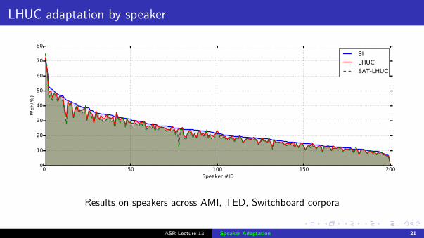
LHUC adaptation by speaker

Results on speakers across AMI, TED, Switchboard corpora


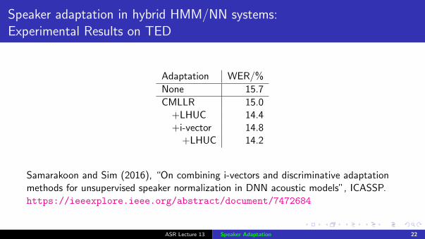
Speaker adaptation in hybrid HMM/NN systems:Experimental Results on TED

Adaptation WER/%

None 15.7

CMLLR 15.0+LHUC 14.4+i-vector 14.8

+LHUC 14.2

Samarakoon and Sim (2016), “On combining i-vectors and discriminative adaptationmethods for unsupervised speaker normalization in DNN acoustic models”, ICASSP.https://ieeexplore.ieee.org/abstract/document/7472684


https://ieeexplore.ieee.org/abstract/document/7472684

Summary

Speaker Adaptation

An intensive area of speech recognition research since the early 1990s

HMM/GMM

Substantial progress, resulting in significant, additive, consistent reductions in worderror rateClose mathematical links between different approachesLinear transforms at the heart of many approachesMLLR family is very effective

HMM/NN

Open research topicGMM-based feature space transforms (CMLLR), i-vectors, and LHUC are effective(and complementary)


Reading

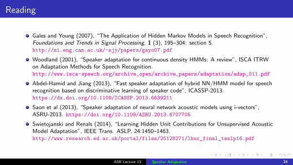
Gales and Young (2007), “The Application of Hidden Markov Models in Speech Recognition”,Foundations and Trends in Signal Processing, 1 (3), 195–304: section 5.http://mi.eng.cam.ac.uk/~sjy/papers/gayo07.pdf

Woodland (2001), “Speaker adaptation for continuous density HMMs: A review”, ISCA ITRWon Adaptation Methods for Speech Recognition.http://www.isca-speech.org/archive_open/archive_papers/adaptation/adap_011.pdf

Abdel-Hamid and Jiang (2013), “Fast speaker adaptation of hybrid NN/HMM model for speechrecognition based on discriminative learning of speaker code”, ICASSP-2013.https://dx.doi.org/10.1109/ICASSP.2013.6639211

Saon et al (2013), “Speaker adaptation of neural network acoustic models using i-vectors”,ASRU-2013. https://doi.org/10.1109/ASRU.2013.6707705

Swietojanski and Renals (2014), “Learning Hidden Unit Contributions for Unsupervised AcousticModel Adaptation”, IEEE Trans. ASLP, 24:1450–1463.http://www.research.ed.ac.uk/portal/files/25128271/lhuc_final_taslp16.pdf


http://mi.eng.cam.ac.uk/~sjy/papers/gayo07.pdf

http://www.isca-speech.org/archive_open/archive_papers/adaptation/adap_011.pdf

https://dx.doi.org/10.1109/ICASSP.2013.6639211

https://doi.org/10.1109/ASRU.2013.6707705

http://www.research.ed.ac.uk/portal/files/25128271/lhuc_final_taslp16.pdf

Speaker Adaptation · Speaker adaptation in hybrid HMM/NN systems: Speaker codes Basic idea:Learn a...

Documents

Transcript of Speaker Adaptation · Speaker adaptation in hybrid HMM/NN systems: Speaker codes Basic idea:Learn a...