SPE-149629-PP

Geomagnetic Referencing in the Arctic Environment Benny Poedjono and Nathan Beck, SPE, Schlumberger; and Andrew Buchanan, Jason Brink and Joseph Longo, SPE, Eni Petroleum Co.; and Carol A. Finn and E. William Worthington, U. S. Geological Survey

Copyright 2011, Society of Petroleum Engineers This paper was prepared for presentation at the SPE Arctic and Extreme Environments Conference & Exhibition held in Moscow, Russia, 18–20 October 2011. This paper was selected for presentation by an SPE program committee following review of information contained in an abstract submitted by the author(s). Contents of the paper have not been reviewed by the Society of Petroleum Engineers and are subject to correction by the author(s). The material does not necessarily reflect any position of the Society of Petroleum Engineers, its officers, or members. Electronic reproduction, distribution, or storage of any part of this paper without the written consent of the Society of Petroleum Engineers is prohibited. Permission to reproduce in print is restricted to an abstract of not more than 300 words; illustrations may not be copied. The abstract must contain conspicuous acknowledgment of SPE copyright.

Abstract Geomagnetic referencing is becoming an increasingly attractive alternative to north-seeking gyroscopic surveys to achieve the precise wellbore positioning essential for success in today's complex drilling programs. However, the greater magnitude of variations in the geomagnetic environment at higher latitudes makes the application of geomagnetic referencing in those areas more challenging.

Precise, real-time data on those variations from relatively nearby magnetic observatories can be crucial to achieving the required accuracy, but constructing and operating an observatory in these often harsh environments poses a number of significant challenges. Operational since March 2010, the Deadhorse Magnetic Observatory (DED), located in Deadhorse, Alaska, was created through collaboration between the United States Geological Survey (USGS) and a leading oilfield services supply company. DED was designed to produce real-time geomagnetic data at the required level of accuracy, and to do so reliably under the extreme temperatures and harsh weather conditions often experienced in the area.

The observatory will serve a number of key scientific communities as well as the oilfield drilling industry, and has already played a vital role in the success of several commercial ventures in the area, providing essential, accurate data while offering significant cost and time savings, compared with traditional surveying techniques.

2 SPE-149629-PP

Introduction The geologic setting of the North Slope of Alaska (Fig. 1), and more specifically offshore in the Beaufort Sea, where the Eni Petroleum Nikaitchuq field is located (Fig. 2), is complex. Because of the complex geology of zones of interest in this area, precise, real-time wellbore positioning is essential to the success of commercial development.

A higher degree of accuracy is required to Ensure that wellbores are placed with adequate precision to ensure proper separation of adjacent injectors and

producers Avoid the overlapping of ellipse of uncertainty (EOU) trajectories and possible collision with adjacent wellbores,

which could occur if the conventional MWD survey error model were used A closer look at the geology of the Nikaitchuq field will illustrate the unique challenges involved in locating and producing

its resources. Challenges in Nikaitchuq Field The main reservoirs of the field are the OA and N sands within the Schrader Bluff formation. Minor oil accumulations have been tested in the Triassic “Sag River Sandstones.” The Schrader Bluff formation consists dominantly of marine sandstones and shale deposited within a foreland basin (Colville basin) during the late Cretaceous period. At that time, the source of the sediments was from the southwest, and toward this direction the Schrader Bluff interfingers with the nonmarine or marginal marine sediments of the Prince Creek formation. Toward the basin, far from the sediment source, the Schrader Bluff interfingers with the deeper marine shales of the Canning formation.

During the Tertiary period the fluviodeltaic deposits of the Sagavanirktok formation completely filled up the basin and closed the sedimentary cycle. A total of ten exploratory and/or appraisal wellbores have been drilled within the Nikaitchuq structure. Moreover, seven neighboring wellbores have been considered to build a full-field 3D reservoir model (static and dynamic). Within the multidisciplinary study a detailed sedimentological reinterpretation of the two available Shrader Bluff cored sections has been performed. The Nikaitchuq’s Schrader Bluff OA sands have been interpreted as shelfal lobe deposits.

Starting from the bottom, the first zone represents a distal prodeltaic system characterized by the succession of laminated sand and silt. The overlying deposits were interpreted as mixed depositional system-shelfal lobe complex; this complex consists of turbidite-like facies encased in structural depressions within distal delta-front and prodeltaic deposits. Three different shelfal lobes separated by silty layers or cemented layers rich in calcite were recognized. The closure of the OA sequence has been interpreted as an outer shelf facies association. The Schrader Bluff N sand was interpreted in the same way by analogy, since no cores have ever been cut in the interval. The areal extension of these “turbiditic” bodies was defined by means of wellbore correlation, analogues, and the qualitative interpretation of seismic amplitude maps.

Fig. 1—Nikaitchug geological sequence, source rock intervals and principle reservoirs

SPE-149629-PP 3

Fig. 2—The Nikaitchuq field and location (right) in the North Slope region of Alaska.

For the OA sands, two well tests have been performed (Nikaitchuq 4 and OP-2) to evaluate the production rates, to investigate the reservoir behavior, to evaluate the sand’s petrophysical characteristics, and to collect oil samples. The OA sand hydrocarbons are viscous oil (16 to 19° API with 100 to 180 cp) characterized by a low gas/oil ratio (70-150 scf/STB). No oil samples are available for the N sand.

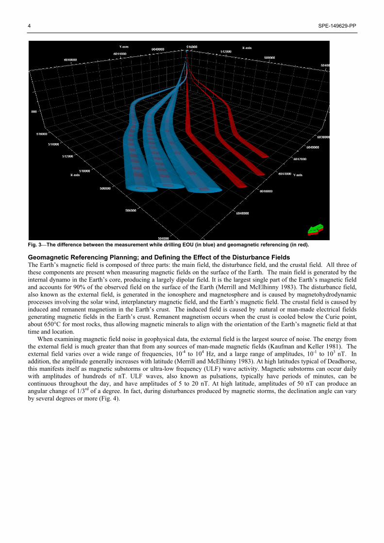
The structural setting of the reservoirs is a monocline, dipping very gently to the northeast. The trap mechanism is structural and stratigraphic. Several “updip” wellbores located south and west from the main Nikaitchuq area record a thin oil-bearing sand or no sand at all at the OA stratigraphic level. The OA field oil/water contact has been detected by log analysis at 4,177 ft true vertical depth subsea (TVDSS) in well Nikaitchuq 2. The continuity of the structure is interrupted, for the most part, by a set of northwest/southeast normal faults associated to the early Cretaceous rifting of the Beaufort Sea. A minor concurrent set of faults, striking northeast/southwest, is also present. Because of the thin development of the OA sand, the presence of continuous faults with throws greater than 30 to 40 ft could represent a tight barrier. Several pieces of evidence lead to a common conclusion that a major compartmentalization is occurring between the Kigun/Tuvaaq and OP-I2 “updip” portion of the field and the “downdip” area delineated by the Nikaitchuq wellbores and OP-I1. Within the two regions, oils with different qualities and properties have been sampled. The possibility of local reservoir compartmentalization must be considered in the planning and execution phase. Why Geomagnetic Referencing is Needed As noted above, precise wellbore positioning is essential to locate and produce the resources in the Nikaitchuq field. Traditional gyroscopic surveys could produce data of sufficient quality to achieve the desired precision of wellbore placement, but the additional costs and time required make them prohibitively expensive for drilling programs in this area. Instead, the decision was made to take advantage of refinements in geomagnetic referencing and the development of a robust geomagnetic referencing processing to provide precise, real-time positioning (Fig. 3). Geomagnetic referencing techniques were deemed capable of addressing the challenges to survey accuracy inherent in high-latitude drilling, particularly the high-disturbance component of Earth’s magnetic field and need to compensate for the effect of drillstring interference.

4 SPE-149629-PP

Fig. 3—The difference between the measurement while drilling EOU (in blue) and geomagnetic referencing (in red). Geomagnetic Referencing Planning; and Defining the Effect of the Disturbance Fields The Earth’s magnetic field is composed of three parts: the main field, the disturbance field, and the crustal field. All three of these components are present when measuring magnetic fields on the surface of the Earth. The main field is generated by the internal dynamo in the Earth’s core, producing a largely dipolar field. It is the largest single part of the Earth’s magnetic field and accounts for 90% of the observed field on the surface of the Earth (Merrill and McElhinny 1983). The disturbance field, also known as the external field, is generated in the ionosphere and magnetosphere and is caused by magnetohydrodynamic processes involving the solar wind, interplanetary magnetic field, and the Earth’s magnetic field. The crustal field is caused by induced and remanent magnetism in the Earth’s crust. The induced field is caused by natural or man-made electrical fields generating magnetic fields in the Earth’s crust. Remanent magnetism occurs when the crust is cooled below the Curie point, about 650°C for most rocks, thus allowing magnetic minerals to align with the orientation of the Earth’s magnetic field at that time and location.

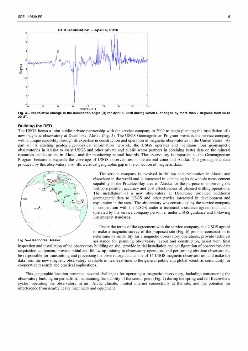
When examining magnetic field noise in geophysical data, the external field is the largest source of noise. The energy from the external field is much greater than that from any sources of man-made magnetic fields (Kaufman and Keller 1981). The external field varies over a wide range of frequencies, 10-4 to 104 Hz, and a large range of amplitudes, 10-1 to 103 nT. In addition, the amplitude generally increases with latitude (Merrill and McElhinny 1983). At high latitudes typical of Deadhorse, this manifests itself as magnetic substorms or ultra-low frequency (ULF) wave activity. Magnetic substorms can occur daily with amplitudes of hundreds of nT. ULF waves, also known as pulsations, typically have periods of minutes, can be continuous throughout the day, and have amplitudes of 5 to 20 nT. At high latitude, amplitudes of 50 nT can produce an angular change of 1/3rd of a degree. In fact, during disturbances produced by magnetic storms, the declination angle can vary by several degrees or more (Fig. 4).

SPE-149629-PP 5

Fig. 4—The relative change in the declination angle (D) for April 5, 2010 during which D changed by more than 7 degrees from 05 to 20 UT.

Building the DED The USGS began a joint public-private partnership with the service company in 2009 to begin planning the installation of a new magnetic observatory at Deadhorse, Alaska (Fig. 5). The USGS Geomagnetism Program provides the service company with a unique capability through its expertise in construction and operation of magnetic observatories in the United States. As part of its existing geologic/geophysical information network, the USGS operates and maintains four geomagnetic observatories in Alaska to assist USGS and other private and public sector partners in obtaining better data on the mineral resources and locations in Alaska and for monitoring natural hazards. The observatory is important to the Geomagnetism Program because it expands the coverage of USGS observatories in the auroral zone and Alaska. The geomagnetic data produced by this observatory also fills a critical geographic gap in the collection of magnetic data.

The service company is involved in drilling and exploration in Alaska and

elsewhere in the world and is interested in enhancing its downhole measurement capability in the Prudhoe Bay area of Alaska for the purpose of improving the wellbore position accuracy and cost effectiveness of planned drilling operations. The installation of a new observatory at Deadhorse provided additional geomagnetic data to USGS and other parties interested in development and exploration in the area. The observatory was constructed by the service company in cooperation with the USGS under a technical assistance agreement, and is operated by the service company personnel under USGS guidance and following Intermagnet standards.

Under the terms of the agreement with the service company, the USGS agreed to make a magnetic survey of the proposed site (Fig. 6) prior to construction to determine its suitability for a magnetic observatory operations, provide technical assistance for planning observatory layout and construction, assist with final

inspection and installation of the observatory building on site, provide initial installation and configuration of observatory data acquisition equipment, provide initial and follow-up training in observatory operations and performing absolute observations, be responsible for transmitting and processing the observatory data as one of 14 USGS magnetic observatories, and make the data from the new magnetic observatory available in near-real-time to the general public and global scientific community for cooperative research and practical applications.

This geographic location presented several challenges for operating a magnetic observatory, including constructing the observatory building on permafrost, maintaining the stability of the sensor piers (Fig. 7) during the spring and fall freeze/thaw cycles, operating the observatory in an Arctic climate, limited internet connectivity at the site, and the potential for interference from nearby heavy machinery and equipment.

Fig. 5—Deadhorse, Alaska

6 SPE-149629-PP

Fig. 6—Magnetic survey conducted by the USGS and the agreed location of the observatory and the communication building.

Fig. 7—Schematic of the observatory showing the location of the sensor piers.

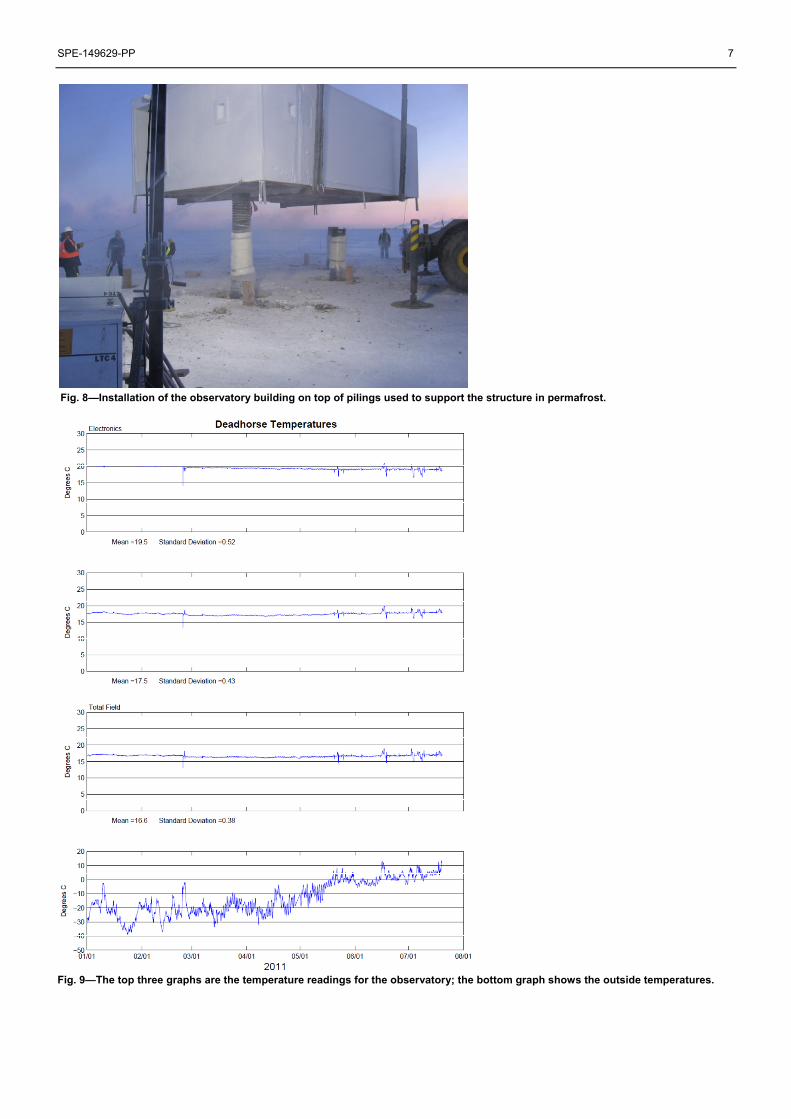
To accommodate construction on the permafrost and in an Arctic environment, the observatory building design included installation on pilings anchored deep in the permanently frozen soil (Fig. 8), an air gap underneath the building to prevent thawing of the permafrost beneath the building, and building insulation adequate to withstand outside temperatures of −40 to –50° and maintain an internal temperature variation of no more than 5°C (Fig. 9).

SPE-149629-PP 7

Fig. 8—Installation of the observatory building on top of pilings used to support the structure in permafrost.

Fig. 9—The top three graphs are the temperature readings for the observatory; the bottom graph shows the outside temperatures.

8 SPE-149629-PP

Operation of the DED A geomagnetic observatory provides accurate records of the Earth’s magnetic field direction and intensity at a given location and over long periods of time. Observatory sites are selected where the horizontal and vertical gradients are less than 3 nT/meter (Jankowski and Sucksdorff 1996). The buildings used for an observatory are constructed of non-magnetic materials so that there are no distortions of the natural magnetic field. The buildings are also isolated inside a perimeter of 80 to 100 m where no vehicles or other possible sources of magnetic disturbances are allowed.

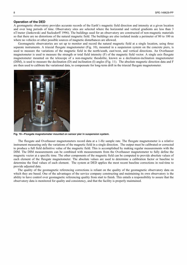
Geomagnetic observatories are set up to monitor and record the natural magnetic field at a single location, using three separate instruments. A triaxial fluxgate magnetometer (Fig. 10), mounted in a suspension system on the concrete piers, is used to measure the variations of the magnetic field in the north/south, east/west, and vertical directions. An Overhauser magnetometer is used to measure the strength or total field intensity (F) of the magnetic field vector. A single axis fluxgate magnetometer mounted on the telescope of a non-magnetic theodolite, known as a declination-inclination magnetometer (DIM), is used to measure the declination (D) and inclination (I) angles (Fig. 11). The absolute magnetic direction data and F are then used to calibrate the variational data, to compensate for long-term drift in the triaxial fluxgate magnetometer.

Fig. 10—Fluxgate magnetometer mounted on sensor pier in suspension system. The fluxgate and Overhauser magnetometers record data at a 1-Hz sample rate. The fluxgate magnetometer is a relative

instrument measuring only the variations of the magnetic field in a single direction. The output must be calibrated or corrected to produce a full field definitive value of the magnetic field. This is accomplished by making regular measurements with the DIM. The DIM measurements can be combined with measurements from the Overhauser magnetometer to fully define the magnetic vector at a specific time. The other components of the magnetic field can be computed to provide absolute values of each element of the fluxgate magnetometer. The absolute values are used to determine a calibration factor or baseline to determine the final values of each element. The system at DED applies the most recent baseline corrections in real-time to provide adjusted data.

The quality of the geomagnetic referencing corrections is reliant on the quality of the geomagnetic observatory data on which they are based. One of the advantages of the service company constructing and maintaining its own observatory is the ability to have control over geomagnetic referencing quality from start to finish. This entails a responsibility to assure that the observatory data is monitored for quality and consistency, and that the facility is properly maintained.

SPE-149629-PP 9

Fig. 11—Non-magnetic theodolite is used weekly to obtain the absolute measurements at DED. Quality Assurance/Quality Control (QA/QC) of DED Data The DED data are transmitted in real time to USGS Geomagnetism Program headquarters in Golden, Colorado via a redundant system consisting of an Internet connection and a series of satellite linkages. The Internet connection at the observatory runs through a 512k nomadic wireless broadband product provided by local internet service provided by GCI. This is the same high quality broadband connection in use at well sites across the Greater Prudhoe Bay.

Weekly measurements of the absolute magnetic field provide the baseline values to ensure the observatory data is properly calibrated. To obtain absolute measurements, specially trained observers visit the observatory on a weekly basis to perform four sets of manual observations using the DIM. These absolute observations are used to compute the magnetometer baselines and then sent to the USGS for analysis, and are used during data processing to apply final adjustments to the vector data. Fig. 12 is an example of one set of the weekly absolute measurements taken by the service company observers.

Fig. 12—Absolute measurements at DED.

Specialized data-processing algorithms have been developed by the USGS in order to produce “definitive” or adjusted data in real time. Since the processing software allows for quick systematic inspection of large quantities of data, it is used for troubleshooting and QA/QC of the observatory data. USGS experts use this process daily to examine all data that comes out of the DED.

10 SPE-149629-PP

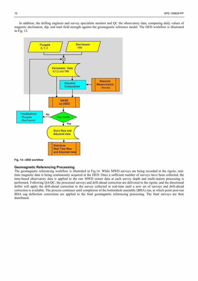
In addition, the drilling engineer and survey specialists monitor and QC the observatory data, comparing daily values of magnetic declination, dip, and total field strength against the geomagnetic reference model. The DED workflow is illustrated in Fig. 13.

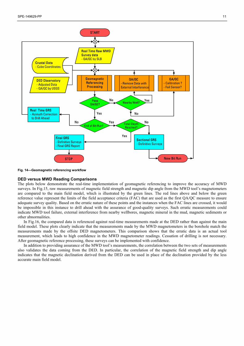
Fig. 13—DED workflow Geomagnetic Referencing Processing The geomagnetic referencing workflow is illustrated in Fig.14. While MWD surveys are being recorded at the rigsite, real-time magnetic data is being continuously acquired at the DED. Once a sufficient number of surveys have been collected, the time-based observatory data is applied to the raw MWD sensor data at each survey depth and multi-station processing is performed. Following QA/QC, the processed surveys and drill-ahead correction are delivered to the rigsite, and the directional driller will apply the drill-ahead correction to the survey collected in real-time until a new set of surveys and drill-ahead correction is available. The process continues until completion of the bottomhole assembly (BHA) run, at which point post-run BHA sag deflection corrections are applied to the final geomagnetic referencing processing. The final surveys are then distributed.

SPE-149629-PP 11

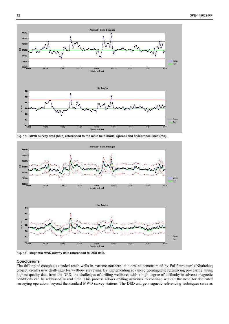
Fig. 14—Geomagnetic referencing workflow DED versus MWD Reading Comparisons The plots below demonstrate the real-time implementation of geomagnetic referencing to improve the accuracy of MWD surveys. In Fig.15, raw measurements of magnetic field strength and magnetic dip angle from the MWD tool’s magnetometers are compared to the main field model, which is illustrated by the green lines. The red lines above and below the green reference value represent the limits of the field acceptance criteria (FAC) that are used as the first QA/QC measure to ensure adequate survey quality. Based on the erratic nature of these points and the instances when the FAC lines are crossed, it would be impossible in this instance to drill ahead with the assurance of good-quality surveys. Such erratic measurements could indicate MWD tool failure, external interference from nearby wellbores, magnetic mineral in the mud, magnetic sediments or other abnormalities.

In Fig.16, the compared data is referenced against real-time measurements made at the DED rather than against the main field model. These plots clearly indicate that the measurements made by the MWD magnetometers in the borehole match the measurements made by the offsite DED magnetometers. This comparison shows that the erratic data is an actual tool measurement, which leads to high confidence in the MWD magnetometer readings. Cessation of drilling is not necessary. After geomagnetic reference processing, these surveys can be implemented with confidence.

In addition to providing assurance of the MWD tool’s measurements, the correlation between the two sets of measurements also validates the data coming from the DED. In particular, the correlation of the magnetic field strength and dip angle indicates that the magnetic declination derived from the DED can be used in place of the declination provided by the less accurate main field model.

12 SPE-149629-PP

Fig. 15—MWD survey data (blue) referenced to the main field model (green) and acceptance lines (red).

Fig. 16—Magnetic MWD survey data referenced to DED data.

Conclusions The drilling of complex extended reach wells in extreme northern latitudes, as demonstrated by Eni Petroleum’s Nitaitchuq project, creates new challenges for wellbore surveying. By implementing advanced geomagnetic referencing processing, using highest-quality data from the DED, the challenges of drilling wellbores with a high degree of difficulty in adverse magnetic conditions can be addressed in real time. This process allows drilling activities to continue without the need for dedicated surveying operations beyond the standard MWD survey stations. The DED and geomagnetic referencing techniques serve as

SPE-149629-PP 13

critical enablers, both ensuring the delivery of geological objectives and minimizing collision risks through enhanced surveying accuracy, all without any cessation in drilling activity. Acknowledgments The authors appreciate the permission of Eni Petroleum, the USGS and Schlumberger for their permission to publish the material contained in this paper. We thank them for their contributions and for ensuring that the operations were safely and successfully executed. We would like to thank J. J. Love of USGS and H. T. Andersen of Digitus International for reviewing a draft manuscript. References Jankowski, J. and Sucksdorff, C., Guide for Magnetic Measurements and Observatory Practice, IAGA: Warsaw, 235 p, 1996. Kaufman, A. A., and Keller, G. V., The Magnetotelluric Sounding Method, Elsevier: New York, 591 p, 1981 Merrill, R. T., and McElhinny, M. W., The Earth’s Magnetic Field, Academic Press: London, 401 p, 1983.