SPC 407

Supersonic & Hypersonic Fluid Dynamics

Ansys Fluent Tutorial 4

Compressible Flow through Convergent Conical

Nozzle

Introcuction The accurate numerical prediction of nozzle flows can be a valuable tool in the evaluation of designs of

propulsion systems of a turbojet aircraft. Broad-spectrum, easy-to-implement numerical models of

turbulent subsonic, transonic and supersonic flows from turbojet engine exhaust nozzles are being sought

to augment the design process of nozzles, which are often of a convergent-conical type, operating at

various nozzle pressure ratios. The flow of an imperfectly expanded supersonic jet exhausted from a

convergent conical nozzle is also complicated by the presence of a quasi-periodic shock-cell structure that

can significantly affect radiated jet noise. It is essential for the analysis to accurately resolve shock-cell

structures of supersonic jets for a comprehensive exhaust flow analysis including jet expansion, mixing, and associated jet noise.

This tutorial discusses the pressure-based coupled algorithm implemented in the general purpose CFD

code ANSYS Fluent, and evaluates its effectiveness in solving axisymmetric problems of steady and

transient flows through convergent conical nozzles at different nozzle pressure ratios.

A pressure-based coupled solver formulation with weighted second-order central-upwind spatial

discretizations (QUICK scheme) is applied to calculate the numerical solutions. A hierarchy of

axisymmetric hybrid computational meshes is constructed to evaluate grid independence. Effects of

turbulence modeling are evaluated by comparing SST k-𝜔 and Renormalization Group (RNG) k- 𝜀 .

Numerical predictions of discharge and thrust coefficients, and Mach numbers inside and at the nozzle

exit are compared with the experimental data and excellent agreements are presented.

APPLICATIONS Aircraft propulsion.

KEY WORDS CFD, nozzle, propulsion, compressible flow

Outline

1. Problem description

2. Numerical model

– Pressure-based coupled solver

– Physical models and boundary conditions

– Computational mesh

3. Numerical results and comparison with

test data

– Steady-state axisymmetric results

– Transient solution of vortex shedding off the

splitter trailing edge

4. Summary

Problem Description

Benchmark problem of the 1st AIAA Propulsion Aerodynamics Workshop (2012)

• nozzle geometry and flow conditions from

experiments of Thornock and Brown1

Axisymmetric nozzle:

• 25 deg cone half angle

• Nozzle exit diameter = 3.0 inches

• Conditions correspond to a stationary nozzle discharging into

a quiescent ambient air at standard sea level ambient

pressure (14.696 psi)

• Cold jets with total temperature and ambient static temperatures of 518.7 R

• Nozzle pressure ratio (NPR) varied from 1.4 to 7.0

– fully expanded jet Mach numbers are subsonic for NPRs 1.4 to 1.8 and

supersonic for NPRs 2.0 to 7.0.

• Nozzle coefficients of thrust, Cv, and discharge, Cd, are determined on the basis of axisymmetric flow computations

• Noise radiation by an axisymmetric supersonic jet at NPR = 2.5 is considered

25 deg

References (included in tutorial Zip File)

1. Thornock, R. L., and Brown, E. F., "An Experimental study of Compressible Flow Through Convergent-Conical Nozzles, Including a Comparison With Theoretical Results," Transactions of the ASME: J. Basic Engineering, 1972, pp. 926-932.

2. Vance F. Dippold, NASA Report, “Computational Simulations of Convergent Nozzles for the AIAA 1st Propulsion Aerodynamics Workshop”, 2014

Simulation Steps

Open ANSYS Workbench

We are ready to do a simulation in ANSYS Workbench! Open ANSYS Workbench by

going to Start > ANSYS > Workbench. This will open the startup screen seen as seen

below

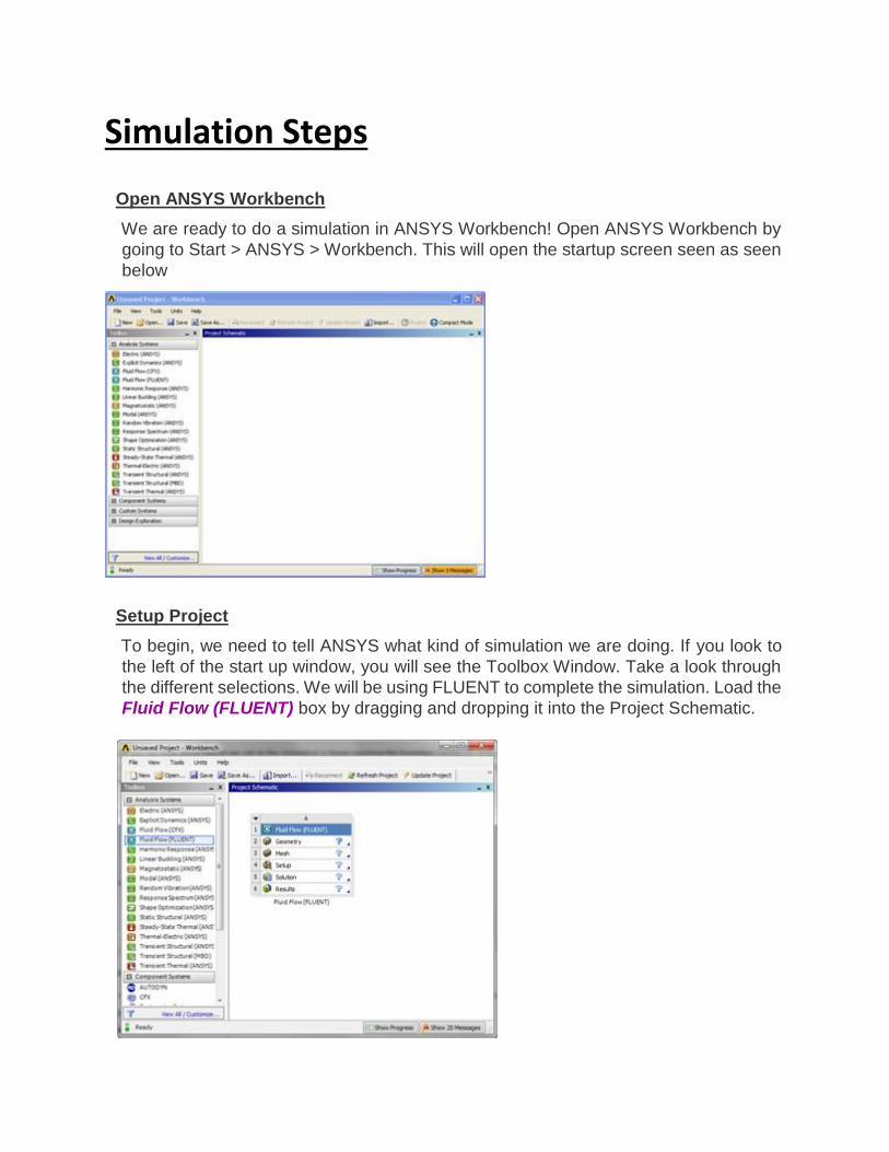
Setup Project

To begin, we need to tell ANSYS what kind of simulation we are doing. If you look to

the left of the start up window, you will see the Toolbox Window. Take a look through

the different selections. We will be using FLUENT to complete the simulation. Load the

Fluid Flow (FLUENT) box by dragging and dropping it into the Project Schematic.

Right click the top box of the project schematic

and go to Rename, and name the project “Conical Divergent Nozzle”. You are ready

to import the case file which include the geometry and the mesh.

Set Up Problem in FLUENT

Right Click on cell “A4” setup >>Import Fluent Case >> Browse>> locate Tut_4_case_file.cas file (located at the same folder of downloaded files)

When the project updates, double click Setup to open FLUENT.

Initial Settings

(Double Click) Setup in the Workbench Project Page.

When the FLUENT Launcher appears change options to "Double Precision", and then click OK as shown below.

Problem Setup - Fluent

Now, FLUENT should open. We will begin setting up some options for the solver. The mesh should be similar to the two figures below

In the left hand window (in what I will call the Outline window), under Problem Setup, select General. The only option we need to change here is the type of 2D space. In the Solver window, select Axisymmetric.

Models

In the outline window, click Models. We will need to utilize the energy equation in order to solve this simulation. Under Models highlight Energy-Off and click Edit Now, the Energy window will launch. Check the box next to Energy Equation and hit OK. Doing this turns on the energy equation.

We also need to change the type of viscosity model. Select Viscous - Laminar and click Edit.... Choose the k-omega and SST under K-omega model option and press OK.

Materials

In the Outline window, highlight Materials. In the Materials window, highlight Fluid, and click Create/Edit.... this will launch the Create/Edit Materials window; here we can specify the properties of the fluid. Set the Density to Ideal Gas, Viscosity to Sutherland and the default values for Cp (1006.43), and the Molecular Weight (28.966) are used. When you have updated these fields, press Change/Create.

• Air modeled as single-species ideal gas

• Molecular viscosity defined as a function of temperature by Sutherland's viscosity law

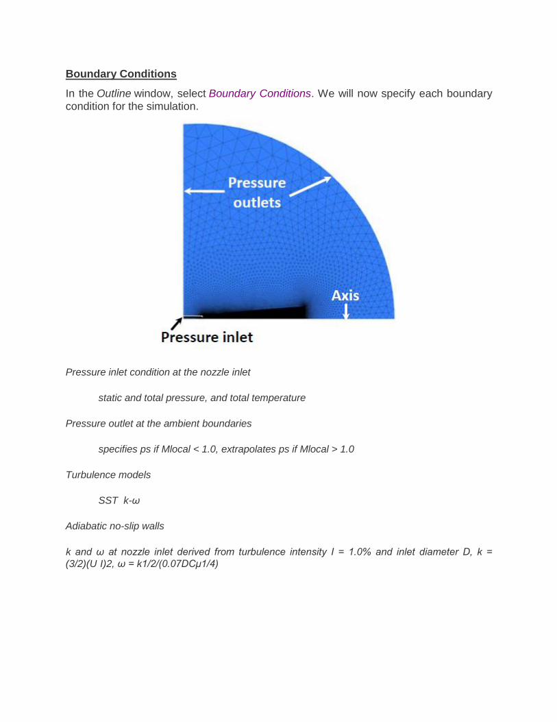
Boundary Conditions

In the Outline window, select Boundary Conditions. We will now specify each boundary condition for the simulation.

Pressure inlet condition at the nozzle inlet

static and total pressure, and total temperature

Pressure outlet at the ambient boundaries

specifies ps if Mlocal < 1.0, extrapolates ps if Mlocal > 1.0

Turbulence models

SST k-ω

Adiabatic no-slip walls

k and ω at nozzle inlet derived from turbulence intensity I = 1.0% and inlet diameter D, k =

(3/2)(U·I)2, ω = k1/2/(0.07DCμ1/4)

Axis

In the Boundary Conditions window, select axis. Use the drop-down menu to make sure that its type is axis.

Axis-Nozzle

In the Boundary Conditions window, select axis-nozzle. Use the drop-down menu to make sure that its type is axis.

Inlet

In the Boundary Conditions window, select inlet. Use the drop-down menu to change the Type to pressure-inlet. You will be asked to confirm the change, and do so by pressing OK. Next, a dialogue box will open with some parameters we need to specify. Change the Gauge Total Pressure (psi) to 58.4838 (equivalent to pressure ratio of 4) and make sure that Initial gauge pressure and Turbulent intensity are 14.6959 and 0.01

respectively.

Also, select the Thermal tab, and ensure that the temperature correctly defaulted to 540 R. When you are finished, press OK.

Outlet

In the Boundary Conditions window, select outlet. Use the drop-down menu to change the Type to pressure-outlet. Keep the gauge pressure at 14.6959 psi, press OK.

Wall-nozzle-in

In the Boundary Conditions window, select wall. Use the drop-down menu to change the Type to wall.

Wall-nozzle-out

In the Boundary Conditions window, select wall. Use the drop-down menu to change the Type to wall.

Operating Conditions

In the Boundary Conditions window, select the Operating Conditions button. Change the Gauge Pressure to 0. Then press OK

It is important to check the operating conditions. When setting the density in materials to ideal gas, FLUENT calculates the density using the absolute pressure. However, the pressure we specify is the gauge pressure, not the absolute pressure. FLUENT will use the absolute pressure to compute the density therefore if we do not set the operating pressure to 0 our density will be incorrect for the flow field.

Reference Values

In the Outline window, select Reference Values. Change the Compute From parameter to inlet. Check that the values are accurate. The reference values are used when calculating the non-dimensional results such as the drag coefficient.

Solution Methods

In the Outline window, select Solution Methods to open the Solution Methods window. Under Scheme, choose coupled, Under Spatial Discretization, ensure that the following options are selected:

Gradient: Least Squares Cell Based.

Pressure: Second Order.

Density: Second Order Upwind.

Momentum: Second Order Upwind.

Turbulent Kinetic Energy: Second Order Upwind.

Specific Dissipation Rate: Second Order Upwind.

Energy: Second Order Upwind.

• Pressure-based coupled solver o pressure field is extracted by solving a pressure correction equation

obtained by manipulating continuity and momentum equations o full implicit coupling between momentum and continuity equations o coupled system solved using coupled algebraic multigrid (AMG) scheme o Incomplete Lower Upper (ILU) smoother to smooth residuals between

levels of AMG

• QUICK scheme for interpolating face values from cell centers in the continuity, momentum and energy equations

o weighted average of 2nd order upwind and 2nd order central differencing o less diffusive than a traditional 2nd order upwind

• Pressure face values interpolated by a 2nd scheme similar to 2nd-order upwinding

• Least Squares cell-based gradient evaluation

• 2nd order spacial accuracy preserved

Solution Controls

In the Outline window, select Solution Controls to open the Solution Controls window. Ensure that the Courant Number is set to 10.0.

Monitors

In the Outline window, click Monitors to open the Monitors window. In the Monitors window, select Residuals - Print,Plot and press Edit.... This will open the Residual Monitors window. We want to change the convergence criteria for our solution. Under Equation and to the right of Continuity, change the Absolute Criteria to 1e-6. Repeat for x-velocity, y-velocity, and energy, then press OK.

Solution Initialization

In the Outline window, select Solution Initialization. We need to make an "Initial Guess" to the solution so FLUENT can iterate to find the final solution. In the Solution Initialization window, select Hybrid Initialization, then press Initialize.

Run Calculation

In the Outline window, select Run Calculation. Change the Number of Iterations to 2000. Double click Calculate to run the calculation. It should a few minutes to solve. After the calculation is complete, save the project. Do not close FLUENT.

Note: 1. You need to run the simulations again by using Realizable K-𝜖 turbulence model and

compare the results with K-w SST Turbulence model.

For the Transient Case

1. Under General, choose Transient

2. Under Solution Methods>> Transient Formulation, use, Second Order Implicit

3. Initialize the flow by using hybrid initialization

4. Under Calculations

• Use a time step of 2 x 10-8 sec and iterate for 10000 time step with max iterations/time step of

150

4. Run Calculations

Computational Meshes

• A hybrid axisymmetric meshes is constructed using ANSYS pre-processing tools

– block-structured quad mesh in the jet flow region, unstructured tri mesh in far field –

boundary layer y+ ≈ 1 mesh at the nozzle walls

Results Effects of NPR, Nozzle Pressure Ratio (Nozzle

Total pressure /Pambient,static) on Mach Number

Mach Number Contours

1. Some calculated parameters are not by default carried over into CFD-post. We are interested in such quantities (i.e. Mach Number). To manually transfer a customized selection of quantities

a. Inside Fluent, Select File > Data File Quantities b. Under Additional Quantities, Select Static Pressure, Total Pressure, Mach Number,

and Total Temperature

2. Run Fluent for one more iteration

3. Post-processing will be done in CFD-post> Right Click Results in Workbench, then update 4. When update is done, Double Click Results in Workbench

5. We are interested in viewing contours of Mach Number in CFD-post a. Select Insert > Contour > Name > Mach No. b. Under Details of Mach No, select Locations > click on the box containing the 3 dots

as shown below, and select fluid in periodic 1 and fluid out periodic 1. c. Variable > Mach Number> No Contours = 101

6. Save a copy of the figure in the graphics pane a. Select the camera icon in the toolbar.

Plot Mach Number Variation Along the center line of the nozzle

First, we'll create a line at the center of the nozzle. Then, we'll plot the Mach number variation along this line using the "Chart" facility in CFD Post.

1. In CFD-post, Insert line at the center of the nozzle. a. Insert> Location > Line

b. Name Line 1 c. Under Details of Velocity vectors, type Point 1 coordinates (-0.574,0,0) and Point 2

coordinates (0.8,0.4,0).

2. Plot Mach Number along the newly created line a. Select Insert > Chart b. Type “Mach no along Line 1” under Name

c. Select the Data Series Tab. Select Location > Line 1.

d. select the X Axis tab. Select Variable > X.

e. select the Y Axis tab. Select Variable > Mach Number.

f. Click Apply to Plot.

g. Export the graph to excel sheet, by clicking export

This file can be opened by excel to calculate the average value if needed.

h. Select the Data Series tab> change the Name to CFD

Add the experimental data to the graph

Add new series by clicking on the new series icon, Name it EXP, Click Apply

Under data Source tab> Select File> import the file named (Exp Mach number along the center - NPR 4)

Under Data Series> line Style (None)> Symbols (Triangle)> Symbol Color Green

Click apply

Results from another paper for different locations are shown below:

Calculating the discharge and Thrust

coefficient of the nozzle The discharge coefficient, Cd (The ratio of the actual mass flow to the ideal mass flow) and thrust

coefficient, CV, (the ratio of the actual thrust to the ideal thrust), were computed for each solution as follows:

The standard discharge coefficient, Cd, and thrust coefficient, CV, are computed over the radius of the

nozzle exit, rjet, using the local density (𝜌), local streamwise velocity (u), and local radius from the

centerline (r). The resultant nozzle exit area, Ajet, was 7.0686 in2. The ideal jet velocity, Ujet, is computed

from the Mach number of the ideally expanded jet, Mjet, and the temperature of the jet, Tjet, all found in

the following equations:

In CFD Post, you should draw a line at the exit of the nozzle point (0,0,0) and point (0,0.038,0) and

calculate the average velocity and average density by exporting the data to an excel file to calculate the

average as shown before.

Calculate the drag and discharge coefficient as follows

𝐶𝑑 =𝜌𝑎𝑣×𝑢𝑎𝑣

𝑃𝑗𝑒𝑡

𝑅 𝑇𝑗𝑒𝑡×𝑈𝑗𝑒𝑡

𝐶𝑉 =2𝜋×𝑢𝑎𝑣×(𝑝𝑎𝑣−𝑝𝑎𝑚𝑏)

𝑈𝑗𝑒𝑡

The values of Mjet and Ujet are shown for each NPR in the following Table

Comparison of Discharge Coefficient Cd

To Calculate the discharge coefficient Cd, you need to use CFD Post to calculate it. This step is left to the

student.

Comparison of Thrust Coefficient Cv

To Calculate the Thrust coefficient Cv, you need to use CFD Post to calculate it. This step is left to the student.

Tutorial Requirement 1. Run the simulation for different Nozzle Pressure Ratios, NPR (Nozzle

Inlet Total pressure /Pambient,static) from 1.4 to 7 as shown below

2. Repeat the simulation by using Realizable K-epsilon turbulence model

and compare the mach contours and Mach values across the center line

of the nozzle results with the k-omega SST turbulence model results.

3. Run the transient case and creat a video the video by using the

method shown below in CFD Post:

https://youtu.be/xQBvYceTg8E?t=898

4. Calculae the thrust and drag coeffiecents for NPR=4 and compare it

with th experimental data (CD=0.95 and CV=.978)

NPR = 1.4

NPR = 4.0 NPR = 2.0

NPR = 5.0

NPR = 1.6 NPR = 1.8

NPR = 3.0

NPR = 6.0 NPR = 7.0

Summary

• Numerical predictions of nozzle coefficients, Mach number distributions and shock location are in excellent agreement with experimental data as shown in the plotted data in this tutorial.

• Pressure-based coupled solver (PBCS) is a robust and effective method for solving subsonic and supersonic nozzle flow problems

– adequately resolves physics and capture all essential features

– less memory and CPU intensive than a traditional density-based

approach

– can be an economically attractive alternative to a density-based

algorithm for obtaining steady-state solutions to subsonic and

supersonic problems

A convergent nozzle will not allow supersonic exit speeds of the

combustion gasses, but due to their high temperature their

speed of sound is considerably higher that of the surrounding

air. For example, at 700°C the speed of sound in air is 625 m/s.

Since thrust is mainly determined by the difference in entry and

exit speeds of the air flowing through an engine, a higher speed

than flight speed is required for positive thrust. Low supersonic

flight speeds are entirely possible with a convergent nozzle.

If the design is meant to fly supersonically, which implicates a

lot of design adaptions, it makes sense to go for higher

supersonic speed; however, this requires both an adjustable

intake and an adjustable convergent-divergent nozzle. Both

increase efficiency, dramatically so at higher Mach numbers.