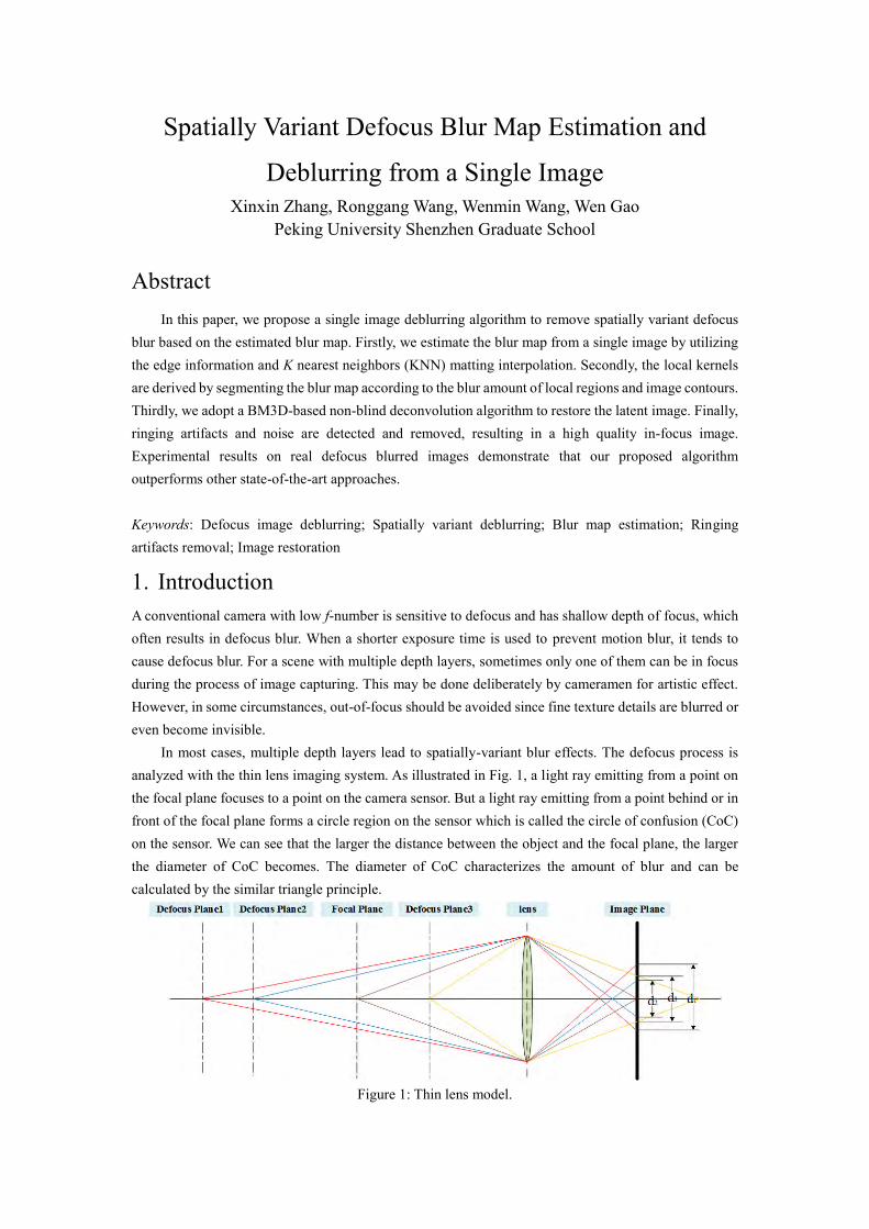
Spatially Variant Defocus Blur Map Estimation and

Deblurring from a Single Image Xinxin Zhang, Ronggang Wang, Wenmin Wang, Wen Gao

Peking University Shenzhen Graduate School

Abstract In this paper, we propose a single image deblurring algorithm to remove spatially variant defocus

blur based on the estimated blur map. Firstly, we estimate the blur map from a single image by utilizing the edge information and K nearest neighbors (KNN) matting interpolation. Secondly, the local kernels are derived by segmenting the blur map according to the blur amount of local regions and image contours. Thirdly, we adopt a BM3D-based non-blind deconvolution algorithm to restore the latent image. Finally, ringing artifacts and noise are detected and removed, resulting in a high quality in-focus image. Experimental results on real defocus blurred images demonstrate that our proposed algorithm outperforms other state-of-the-art approaches.

Keywords: Defocus image deblurring; Spatially variant deblurring; Blur map estimation; Ringing artifacts removal; Image restoration

1. Introduction A conventional camera with low f-number is sensitive to defocus and has shallow depth of focus, which often results in defocus blur. When a shorter exposure time is used to prevent motion blur, it tends to cause defocus blur. For a scene with multiple depth layers, sometimes only one of them can be in focus during the process of image capturing. This may be done deliberately by cameramen for artistic effect. However, in some circumstances, out-of-focus should be avoided since fine texture details are blurred or even become invisible.

In most cases, multiple depth layers lead to spatially-variant blur effects. The defocus process is analyzed with the thin lens imaging system. As illustrated in Fig. 1, a light ray emitting from a point on the focal plane focuses to a point on the camera sensor. But a light ray emitting from a point behind or in front of the focal plane forms a circle region on the sensor which is called the circle of confusion (CoC) on the sensor. We can see that the larger the distance between the object and the focal plane, the larger the diameter of CoC becomes. The diameter of CoC characterizes the amount of blur and can be calculated by the similar triangle principle.

Figure 1: Thin lens model.

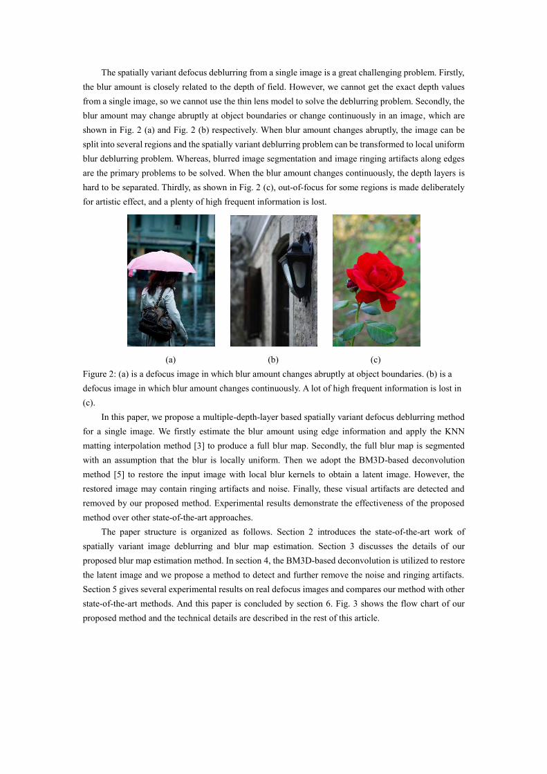
The spatially variant defocus deblurring from a single image is a great challenging problem. Firstly, the blur amount is closely related to the depth of field. However, we cannot get the exact depth values from a single image, so we cannot use the thin lens model to solve the deblurring problem. Secondly, the blur amount may change abruptly at object boundaries or change continuously in an image, which are shown in Fig. 2 (a) and Fig. 2 (b) respectively. When blur amount changes abruptly, the image can be split into several regions and the spatially variant deblurring problem can be transformed to local uniform blur deblurring problem. Whereas, blurred image segmentation and image ringing artifacts along edges are the primary problems to be solved. When the blur amount changes continuously, the depth layers is hard to be separated. Thirdly, as shown in Fig. 2 (c), out-of-focus for some regions is made deliberately for artistic effect, and a plenty of high frequent information is lost.

(a) (b) (c) Figure 2: (a) is a defocus image in which blur amount changes abruptly at object boundaries. (b) is a defocus image in which blur amount changes continuously. A lot of high frequent information is lost in (c).

In this paper, we propose a multiple-depth-layer based spatially variant defocus deblurring method for a single image. We firstly estimate the blur amount using edge information and apply the KNN matting interpolation method [3] to produce a full blur map. Secondly, the full blur map is segmented with an assumption that the blur is locally uniform. Then we adopt the BM3D-based deconvolution method [5] to restore the input image with local blur kernels to obtain a latent image. However, the restored image may contain ringing artifacts and noise. Finally, these visual artifacts are detected and removed by our proposed method. Experimental results demonstrate the effectiveness of the proposed method over other state-of-the-art approaches.

The paper structure is organized as follows. Section 2 introduces the state-of-the-art work of spatially variant image deblurring and blur map estimation. Section 3 discusses the details of our proposed blur map estimation method. In section 4, the BM3D-based deconvolution is utilized to restore the latent image and we propose a method to detect and further remove the noise and ringing artifacts. Section 5 gives several experimental results on real defocus images and compares our method with other state-of-the-art methods. And this paper is concluded by section 6. Fig. 3 shows the flow chart of our proposed method and the technical details are described in the rest of this article.

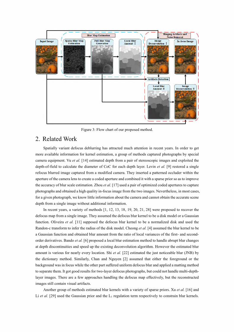
Figure 3: Flow chart of our proposed method.

2. Related Work Spatially variant defocus deblurring has attracted much attention in recent years. In order to get

more available information for kernel estimation, a group of methods captured photographs by special camera equipment. Vu et al. [14] estimated depth from a pair of stereoscopic images and exploited the depth-of-field to calculate the diameter of CoC for each depth layer. Levin et al. [9] restored a single refocus blurred image captured from a modified camera. They inserted a patterned occluder within the aperture of the camera lens to create a coded aperture and combined it with a sparse prior so as to improve the accuracy of blur scale estimation. Zhou et al. [17] used a pair of optimized coded apertures to capture photographs and obtained a high quality in-focus image from the two images. Nevertheless, in most cases, for a given photograph, we know little information about the camera and cannot obtain the accurate scene depth from a single image without additional information.

In recent years, a variety of methods [1, 12, 13, 18, 19, 20, 21, 28] were proposed to recover the defocus map from a single image. They assumed the defocus blur kernel to be a disk model or a Gaussian function. Oliveira et al. [11] supposed the defocus blur kernel to be a normalized disk and used the Randon-c transform to infer the radius of the disk model. Cheong et al. [4] assumed the blur kernel to be a Gaussian function and obtained blur amount from the ratio of local variances of the first- and second-order derivatives. Bando et al. [6] proposed a local blur estimation method to handle abrupt blur changes at depth discontinuities and speed up the existing deconvolution algorithm. However the estimated blur amount is various for nearly every location. Shi et al. [22] estimated the just noticeable blur (JNB) by the dictionary method. Similarly, Chan and Nguyen [2] assumed that either the foreground or the background was in focus while the other part suffered uniform defocus blur and applied a matting method to separate them. It got good results for two-layer defocus photographs, but could not handle multi-depth-layer images. There are a few approaches handling the defocus map effectively, but the reconstructed images still contain visual artifacts.

Another group of methods estimated blur kernels with a variety of sparse priors. Xu et al. [16] and Li et al. [29] used the Gaussian prior and the L1 regulation term respectively to constrain blur kernels.

This kernel estimation algorithm was effective for motion blur kernel estimation, but it was not suitable for defocus blur kernel estimation since the defocus kernels were not sparse enough. Hu et al. [23] extracted depth layers and removed blur by an expectation-maximization (EM) scheme. Though different depth layers could be separated precisely, it depended on user intervention and could not process the blurred image with continuous depth changes well.

3. Blur map estimation The defocus blur degradation can be modeled as a convolution process,

𝐼 = 𝐿⨂𝑘 + 𝑁, (1) where I and L represent the blurred image and in-focus image respectively, ⨂ denotes the convolution operator, N is the unknown sensor noise assumed to be zero-mean Gaussian noise and k is the blur kernel which is approximately considered as a Gaussian function:

𝑘(𝑥, 𝑦, 𝜎) =1

√2𝜋𝜎𝑒

−𝑥2+𝑦2

2𝜎2 , (2)

where (𝑥, 𝑦) represents the coordinate. σ is the standard deviation proportional to the diameter of CoC which measures the defocus blur amount. In spatially variant defocus images, the blur kernels are various in different areas and they are related to the depth of local area. In order to recover L, we should estimate the σ in k firstly.

3.1 Sparse blur map estimation Generally, defocus reduces the edge sharpness and the contrast of the image. When the defocus image is re-blurred, the amount of blur changes significantly at high frequency locations. Thus we estimate the defocus blur at edge locations firstly. The edge in a sharp image can be modeled as:

𝑓(𝑥, 𝑦) = 𝐴𝑢(𝑥, 𝑦) + 𝐵, (3) where 𝑢(𝑥, 𝑦) is the step function, A and B are the amplitude and offset respectively. The location (𝑥, 𝑦) of edge is set as (0,0). We re-blur the edges of I and measure the change of edge information to estimate the edge sharpness. We define the sharpness as:

S =|∇𝐼|−|∇𝐼𝑅|

|∇𝐼|+, (4)

where |∇I| and ∇𝐼𝑅 are the gradient magnitudes of defocus image and re-blurred image respectively, ε is a small positive number to prevent division by zero and |∇I| = √∇𝑥𝐼2 + ∇𝑦𝐼2 , |∇𝐼𝑅| =

√∇𝑥𝐼𝑅2 + ∇𝑦𝐼𝑅

2. The larger the S is, the sharper the edge would be. The sharpness map is shown in Fig.

4 (b). ∇𝐼𝑅 can be expressed as:

|∇𝐼𝑅(𝑥, 𝑦)| = |∇((𝐴𝑢(𝑥, 𝑦) + 𝐵)⨂𝑘(𝑥, 𝑦, 𝜎)⨂𝑘(𝑥, 𝑦, 𝜎0))| =1

√2𝜋(𝜎2+𝜎02)

𝑒−

𝑥2+𝑦2

2(𝜎2+𝜎02), (5)

where 𝜎0 is the standard deviation of the re-blurred kernel. As ε is much smaller than |∇I|, it can be ignored during the calculation, thus (4) can be re-written as:

S = 1 − √𝜎2

𝜎2+𝜎02 𝑒

𝑥2+𝑦2

2𝜎2 −𝑥2+𝑦2

2(𝜎2+𝜎02). (6)

The Canny operator is used to detect edges. Since at edge locations: (𝑥, 𝑦) = (0,0), so,

S = 1 − √𝜎2

𝜎2+𝜎02. (7)

The blur amount σ is expressed by:

σ = √(1−𝑆)2𝜎0

2

2𝑆−𝑆2 . (8)

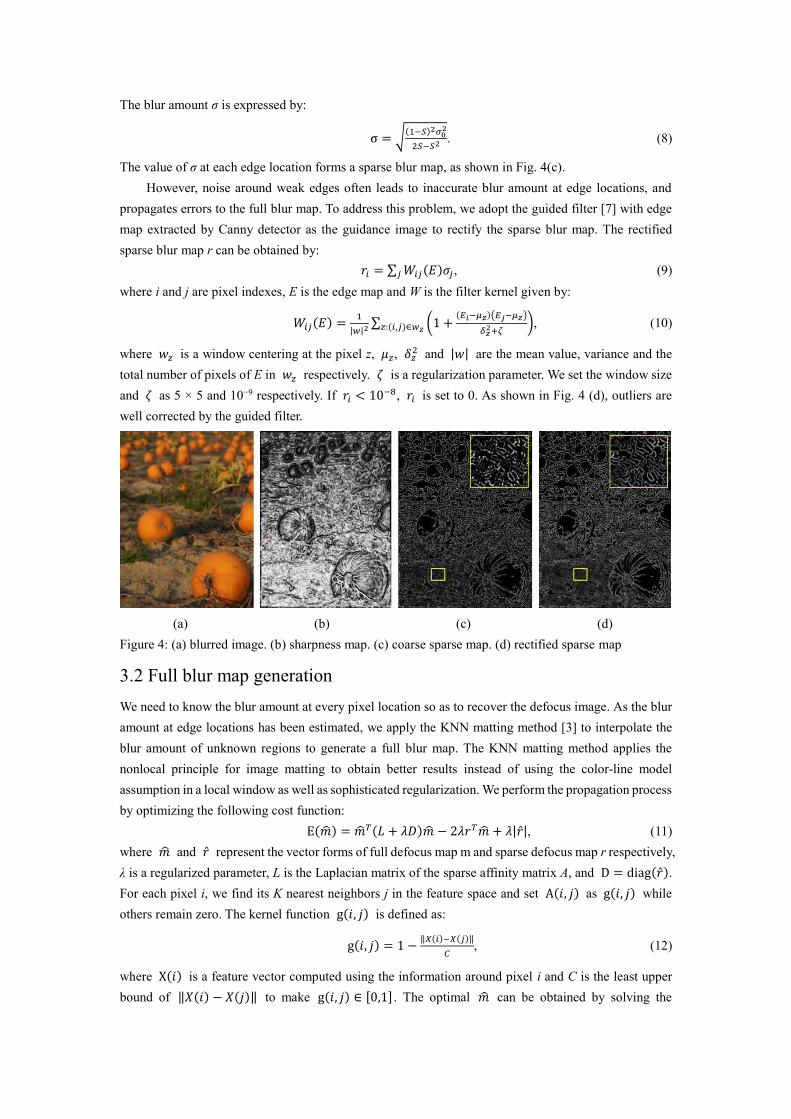
The value of σ at each edge location forms a sparse blur map, as shown in Fig. 4(c). However, noise around weak edges often leads to inaccurate blur amount at edge locations, and

propagates errors to the full blur map. To address this problem, we adopt the guided filter [7] with edge map extracted by Canny detector as the guidance image to rectify the sparse blur map. The rectified sparse blur map r can be obtained by:

𝑟𝑖 = ∑ 𝑊𝑖𝑗(𝐸)𝜎𝑗𝑗 , (9) where i and j are pixel indexes, E is the edge map and W is the filter kernel given by:

𝑊𝑖𝑗(𝐸) =1

|𝑤|2∑ (1 +

(𝐸𝑖−𝜇𝑧)(𝐸𝑗−𝜇𝑧)

𝛿𝑧2+

)𝑧:(𝑖,𝑗)∈𝑤𝑧, (10)

where 𝑤𝑧 is a window centering at the pixel z, 𝜇𝑧, 𝛿𝑧2 and |𝑤| are the mean value, variance and the

total number of pixels of E in 𝑤𝑧 respectively. 𝜁 is a regularization parameter. We set the window size and 𝜁 as 5 × 5 and 10−9 respectively. If 𝑟𝑖 < 10−8, 𝑟𝑖 is set to 0. As shown in Fig. 4 (d), outliers are well corrected by the guided filter.

(a) (b) (c) (d)

Figure 4: (a) blurred image. (b) sharpness map. (c) coarse sparse map. (d) rectified sparse map

3.2 Full blur map generation We need to know the blur amount at every pixel location so as to recover the defocus image. As the blur amount at edge locations has been estimated, we apply the KNN matting method [3] to interpolate the blur amount of unknown regions to generate a full blur map. The KNN matting method applies the nonlocal principle for image matting to obtain better results instead of using the color-line model assumption in a local window as well as sophisticated regularization. We perform the propagation process by optimizing the following cost function:

E(�̂�) = �̂�𝑇(𝐿 + 𝜆𝐷)�̂� − 2𝜆𝑟𝑇�̂� + 𝜆|�̂�|, (11) where �̂� and �̂� represent the vector forms of full defocus map m and sparse defocus map r respectively, λ is a regularized parameter, L is the Laplacian matrix of the sparse affinity matrix A, and D = diag(�̂�). For each pixel i, we find its K nearest neighbors j in the feature space and set A(𝑖, 𝑗) as g(𝑖, 𝑗) while others remain zero. The kernel function g(𝑖, 𝑗) is defined as:

g(𝑖, 𝑗) = 1 −‖𝑋(𝑖)−𝑋(𝑗)‖

𝐶, (12)

where X(𝑖) is a feature vector computed using the information around pixel i and C is the least upper bound of ‖𝑋(𝑖) − 𝑋(𝑗)‖ to make g(𝑖, 𝑗) ∈ [0,1] . The optimal �̂� can be obtained by solving the

following equation: (𝐿 + 𝜆𝐷)�̂� = 𝜆�̂�. (13)

We set λ to 0.8 in our implementation so that �̂� is softly constrained by �̂�. This optimal solution can be solved efficiently by the preconditioned conjugate gradient (PCG) method. The full defocus map is shown in the third box (Full Blur Map Generation) in Fig. 3. We can see that the estimated blur amount increases from the bottom to the top of the image, which is roughly consistent with the depth change.

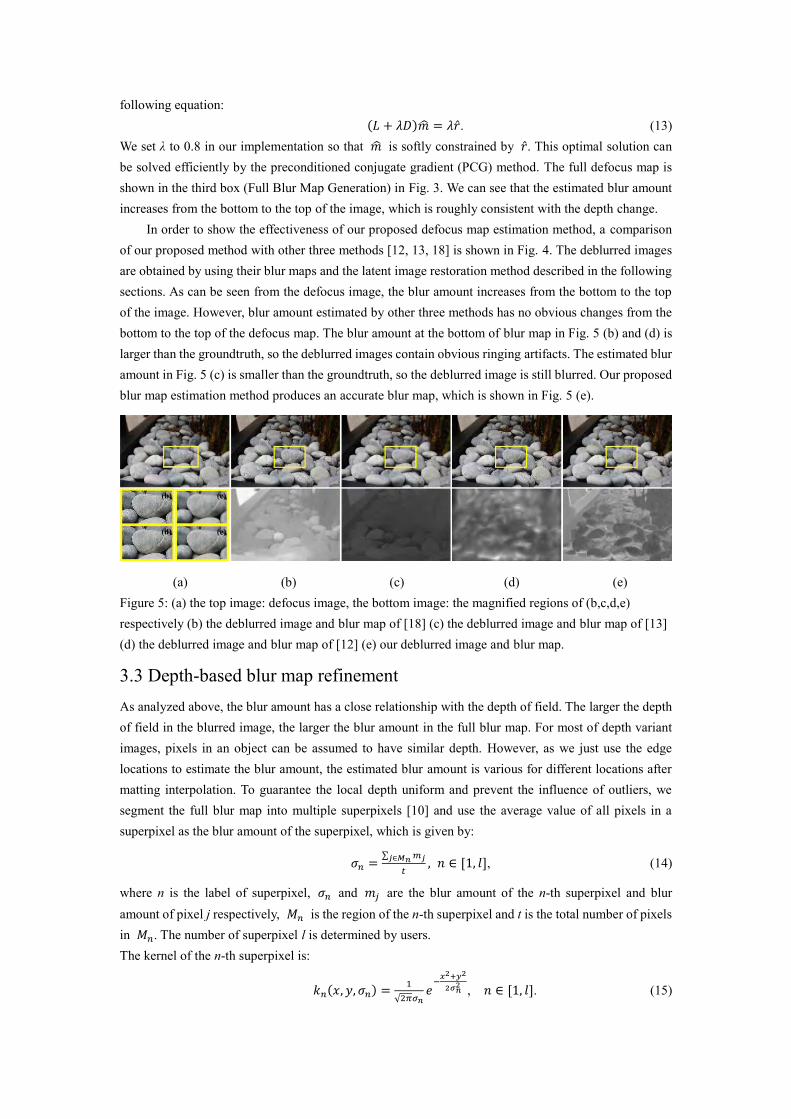
In order to show the effectiveness of our proposed defocus map estimation method, a comparison of our proposed method with other three methods [12, 13, 18] is shown in Fig. 4. The deblurred images are obtained by using their blur maps and the latent image restoration method described in the following sections. As can be seen from the defocus image, the blur amount increases from the bottom to the top of the image. However, blur amount estimated by other three methods has no obvious changes from the bottom to the top of the defocus map. The blur amount at the bottom of blur map in Fig. 5 (b) and (d) is larger than the groundtruth, so the deblurred images contain obvious ringing artifacts. The estimated blur amount in Fig. 5 (c) is smaller than the groundtruth, so the deblurred image is still blurred. Our proposed blur map estimation method produces an accurate blur map, which is shown in Fig. 5 (e).

(a) (b) (c) (d) (e) Figure 5: (a) the top image: defocus image, the bottom image: the magnified regions of (b,c,d,e) respectively (b) the deblurred image and blur map of [18] (c) the deblurred image and blur map of [13] (d) the deblurred image and blur map of [12] (e) our deblurred image and blur map.

3.3 Depth-based blur map refinement As analyzed above, the blur amount has a close relationship with the depth of field. The larger the depth of field in the blurred image, the larger the blur amount in the full blur map. For most of depth variant images, pixels in an object can be assumed to have similar depth. However, as we just use the edge locations to estimate the blur amount, the estimated blur amount is various for different locations after matting interpolation. To guarantee the local depth uniform and prevent the influence of outliers, we segment the full blur map into multiple superpixels [10] and use the average value of all pixels in a superpixel as the blur amount of the superpixel, which is given by:

𝜎𝑛 =∑ 𝑚𝑗𝑗∈𝑀𝑛

𝑡, 𝑛 ∈ [1, 𝑙], (14)

where n is the label of superpixel, 𝜎𝑛 and 𝑚𝑗 are the blur amount of the n-th superpixel and blur amount of pixel j respectively, 𝑀𝑛 is the region of the n-th superpixel and t is the total number of pixels in 𝑀𝑛. The number of superpixel l is determined by users. The kernel of the n-th superpixel is:

𝑘𝑛(𝑥, 𝑦, 𝜎𝑛) =1

√2𝜋𝜎𝑛𝑒

−𝑥2+𝑦2

2𝜎𝑛2 , 𝑛 ∈ [1, 𝑙]. (15)

Then the spatially variant deblurring can be transformed to a local spatially-invariant deblurring problem in each superpixel. We recover each superpixel respectively and stitch the deblurred results to obtain a sharp image. As shown in the fourth box (Local Blur Amount I) in Fig. 3 (f), the superpixel-based segmentation method conforms to the depth of the scene and object edges.

Compared with other local kernel generation methods of blur scale discretion [12] and dividing images into several equal rectangular regions based on kernel similarity [8, 15, 16], our defocus map refinement method produces sharper latent images with much more texture details. The scale selection method [12] selects the biggest quantized blur scale which is smaller than the actual blur amount to generate blur kernels. Though ringing artifacts can be suppressed, the restored images still contain much blur. The simple local kernel estimation [8, 15, 16] ignore the influence of depth and scenes, so areas with different blur amount may be regarded as local uniform.

4. Latent image restoration In this section, we use two steps to obtain the final in-focus image. The first step is to restore the defocus image by non-blind deconvolution. The second step is to remove ringing artifacts and noise using a method based on image re-blurring.

4.1 Non-blind image deconvolution After estimating the full defocus map, we apply a non-blind deconvolution method [5] with regularized inversion and an extended BM3D denoising filter to restore the defocus image. This deblurring algorithm contains two steps. The first step is a regularized inversion using BM3D with collaborative hard-thresholding and the second step is a regularized Wiener inversion using BM3D with collaborative Wiener filtering. The concrete details can be seen in [5]. The strength of this method is that it can remove blur and colored noise efficiently. As described above, we get l local kernels corresponding to l superpixels after segmenting the full blur map. We obtain total l deblurred images by deconvolving the defocus image with 𝑘𝑛(𝑥, 𝑦, 𝜎𝑛) and stitch the corresponding deblurred regions to form an in-focus image L as follows:

L = ∑ �̃�𝑛(𝑥, 𝑦)𝑙𝑛=1 , (16)

where

�̃�𝑛(𝑥, 𝑦) = {�̃�𝑛(𝑥, 𝑦) (𝑥, 𝑦) ∈ 𝑀𝑛

0 𝑜𝑡ℎ𝑒𝑟𝑠, (17)

�̃�𝑛 is the restoration image with 𝑘𝑛.

4.2 Latent image refinement In most cases the BM3D-based deconvolution method can obtain a satisfactory result, while sometimes serious ringing artifacts and noise can be found around the edges. The estimated blur amount which is much larger than the actual blur amount tends to produce ringing artifacts. There are two main reasons leading to this phenomenon. The first one is the improper parameter setting in the superpixels segmentation step. If l were set too small, one superpixel would contain a wide range of depth. Another reason is that the initial estimated blur amount σ of tiny structures is much smaller than the local blur amount 𝜎𝑛.

To address this problem, we propose an efficient method to detect and remove ringing artifacts and noise. We reblur the deblurred superpixel with the corresponding local blur kernel and use deviations to detect ringing artifacts and noise. The deviations between the reblurred image and input image are much

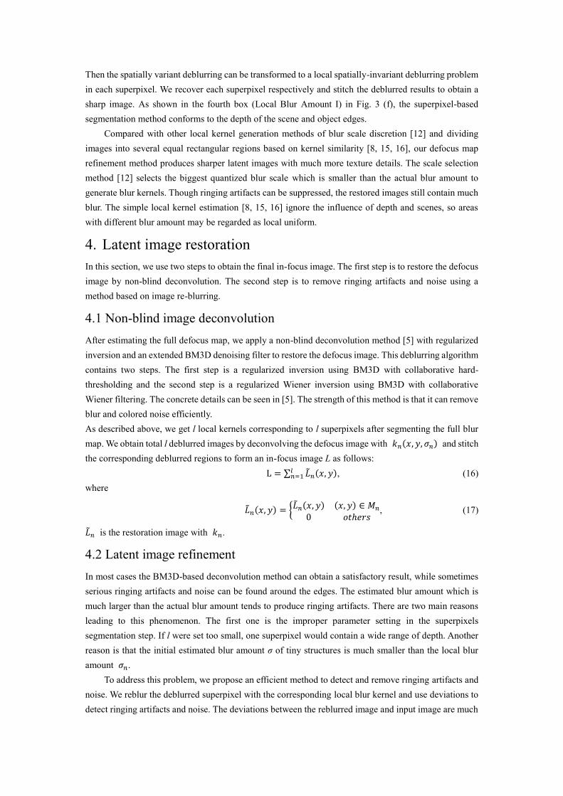
larger in ringing artifacts areas than other areas. The deviation is given by the following formula: e(𝑥, 𝑦) = |�̃�𝑛(𝑥, 𝑦)⨂𝑘𝑛(𝑥, 𝑦, 𝜎𝑛) − 𝐼(𝑥, 𝑦)|, (𝑥, 𝑦) ∈ 𝑀𝑛. (18)

If e(𝑥, 𝑦) is larger than a threshold τ, the corresponding pixel will be supposed to be an outlier. When 𝜎𝑛 is much larger than the blur amount 𝑚𝑗 of a pixel j, the ringing artifacts are detected. So we restore the image with the minimum blur amount in 𝑀𝑛 to create a local kernel (Local Blur Amount II part in Fig. 3) and get an in-focus image �̅�𝑛 (Image Deconvolution II part in Fig. 3). Ringing artifacts and noise are substituted with the recovered pixels in �̅�𝑛, and the visual artifacts are alleviated (the red dotted line box in Fig. 3). The final restored latent image is obtained by:

𝐿𝑓(𝑥, 𝑦) = {�̃�(𝑥, 𝑦) e(𝑥, 𝑦) > 𝜏

�̅�(𝑥, 𝑦) e(𝑥, 𝑦) ≤ 𝜏. (19)

By comparing Fig. 6 (d) with (c), we can see that most of the ringing artifacts are removed.

(a) (b) (c) (d)

Figure 6: (a) blurred image. (b) defocus map. (c) recovered latent image by non-blind deconvolution (d) the final in-focus image.

5. Experimental results In this section, extensive experiments of blur map estimation and image deblurring are performed on several defocus blurred images with our proposed method. In this experiment, we set 𝜎0 = 3 and ε =

10−6 to reblur the defocus image. The number of superpixels l in the full defocus map segmentation is a depth and content dependent parameter which can be tuned by the user. The threshold τ is set to 0.0008.

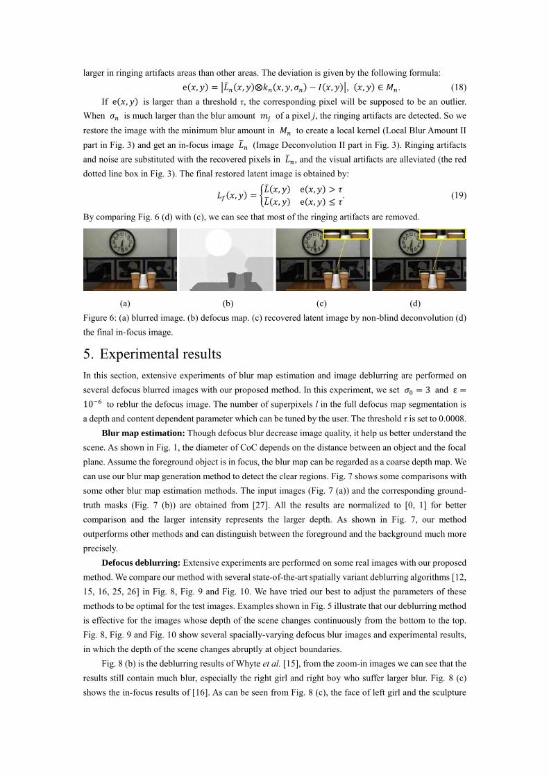
Blur map estimation: Though defocus blur decrease image quality, it help us better understand the scene. As shown in Fig. 1, the diameter of CoC depends on the distance between an object and the focal plane. Assume the foreground object is in focus, the blur map can be regarded as a coarse depth map. We can use our blur map generation method to detect the clear regions. Fig. 7 shows some comparisons with some other blur map estimation methods. The input images (Fig. 7 (a)) and the corresponding ground-truth masks (Fig. 7 (b)) are obtained from [27]. All the results are normalized to [0, 1] for better comparison and the larger intensity represents the larger depth. As shown in Fig. 7, our method outperforms other methods and can distinguish between the foreground and the background much more precisely.

Defocus deblurring: Extensive experiments are performed on some real images with our proposed method. We compare our method with several state-of-the-art spatially variant deblurring algorithms [12, 15, 16, 25, 26] in Fig. 8, Fig. 9 and Fig. 10. We have tried our best to adjust the parameters of these methods to be optimal for the test images. Examples shown in Fig. 5 illustrate that our deblurring method is effective for the images whose depth of the scene changes continuously from the bottom to the top. Fig. 8, Fig. 9 and Fig. 10 show several spacially-varying defocus blur images and experimental results, in which the depth of the scene changes abruptly at object boundaries.

Fig. 8 (b) is the deblurring results of Whyte et al. [15], from the zoom-in images we can see that the results still contain much blur, especially the right girl and right boy who suffer larger blur. Fig. 8 (c) shows the in-focus results of [16]. As can be seen from Fig. 8 (c), the face of left girl and the sculpture

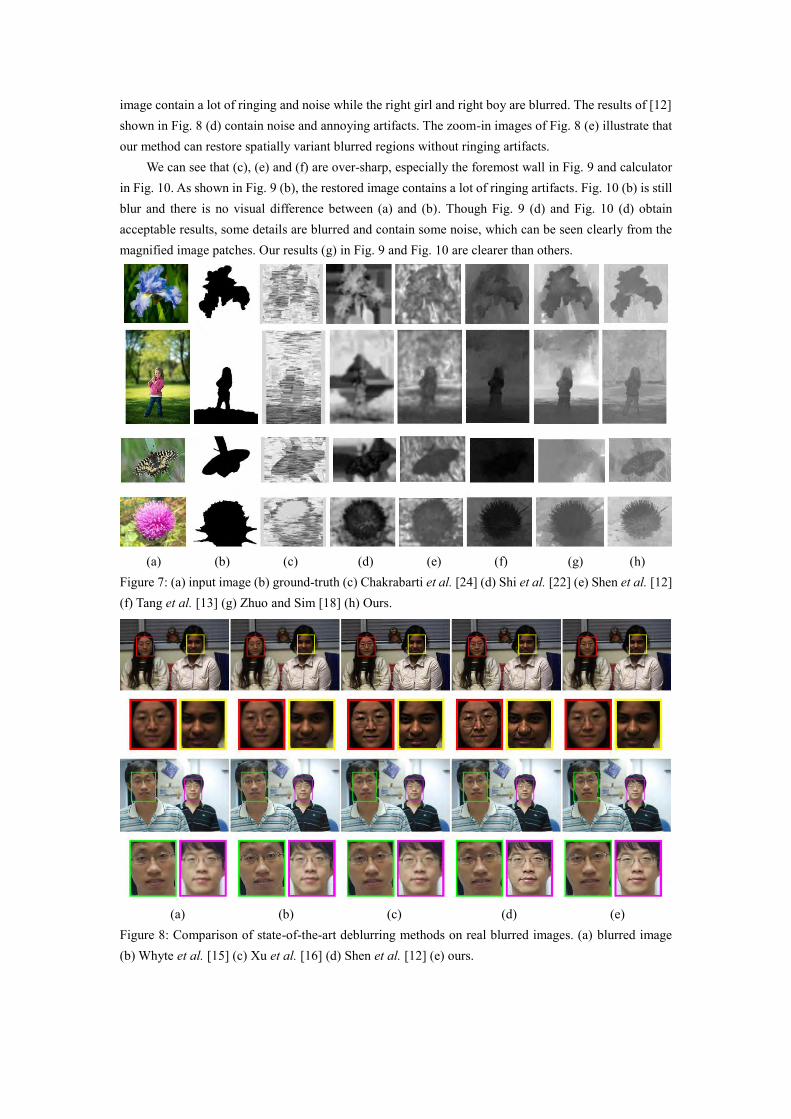
image contain a lot of ringing and noise while the right girl and right boy are blurred. The results of [12] shown in Fig. 8 (d) contain noise and annoying artifacts. The zoom-in images of Fig. 8 (e) illustrate that our method can restore spatially variant blurred regions without ringing artifacts.

We can see that (c), (e) and (f) are over-sharp, especially the foremost wall in Fig. 9 and calculator in Fig. 10. As shown in Fig. 9 (b), the restored image contains a lot of ringing artifacts. Fig. 10 (b) is still blur and there is no visual difference between (a) and (b). Though Fig. 9 (d) and Fig. 10 (d) obtain acceptable results, some details are blurred and contain some noise, which can be seen clearly from the magnified image patches. Our results (g) in Fig. 9 and Fig. 10 are clearer than others.

(a) (b) (c) (d) (e) (f) (g) (h)

Figure 7: (a) input image (b) ground-truth (c) Chakrabarti et al. [24] (d) Shi et al. [22] (e) Shen et al. [12] (f) Tang et al. [13] (g) Zhuo and Sim [18] (h) Ours.

(a) (b) (c) (d) (e)

Figure 8: Comparison of state-of-the-art deblurring methods on real blurred images. (a) blurred image (b) Whyte et al. [15] (c) Xu et al. [16] (d) Shen et al. [12] (e) ours.

(a) (b) (c) (d) (e) (f) (g) Figure 9: Comparison of state-of-the-art deblurring methods on real blurred images. (a) blurred image (b) Whyte et al. [15] (c) Xu et al. [16] (d) Shen et al. [12] (e) Hu and Yang [26] (f) Whyte et al. [25] (g) ours.

Figure 10: Comparison of state-of-the-art deblurring methods on real blurred images. (a) blurred image (b) Whyte et al. [15] (c) Xu et al. [16] (d) Shen et al. [12] (e) Hu and Yang [26] (f) Whyte et al. [25] (g) ours.

6. Conclusion In this work, a robust spatially variant defocus deblurring method is proposed. This paper has three main contributions. Firstly, we propose a novel method to estimate the blur map from a single image by utilizing the change of edge information and KNN matting interpolation. Secondly, local blur kernels are derived by segmenting the defocus map with our depth local uniform assumption. Thirdly, we propose an efficient ringing artifacts and de-noising method to improve the latent image quality. Experimental results over several images show the effectiveness of our method.

Reference [1] S. Bae and F. Durand. Defocus magnification. Computer Graphics Forum, 26(3) (2007) 571-579. [2] S. H. Chan and T. Q. Nguyen. Single image spatially variant out-of-focus blur removal. In IEEE International Conference on Image Processing (ICIP), 2011, pp. 677-680. [3] Q. Chen, D. Li, and C. K. Tang. Knn matting. Pattern Recognition, 35(9) (2013) 2175-2188. [4] H. Cheong, E. Chae, E. Lee, G. Jo, and J. Paik. Fast image restoration for spatially varying defocus blur of imaging sensor. Sensors, 15(1) (2015) 880-898. [5] K. Dabov, A. Foi, V. Katkovnik, and K. Egiazarian. Image restoration by sparse 3d transform-domain collaborative filtering. In Electronic Imaging 2008. International Society for Optics and Photonics (SPIE Electronic Imaging), 2008, pp. 681207-681207-12. [6] J. Dorsey, S. Xu, G. Smedresman, H. Rushmeier, and L. McMillan. Towards digital refocusing from a single photograph. In Computer Graphics and Application (PG’07), 2007, pp. 363-372. [7] K. He, J. Sun, and X. Tang. Guided image filtering. Lecture Notes in Computer Science, 35(6) (2010) 1–14. [8] Z. Hu and M. H. Yang. Fast non-uniform deblurring using constrained camera pose subspace. In British Machine Vision Conference (BMVC), 2012, pp. 1-11. [9] A. Levin, R. Fergus, F. Durand, and W. T. Freeman. Image and depth from a conventional camera with a coded aperture. ACM Transactions on Graphics, 26(3) (2007) 70. [10] G. Mori. Guiding model search using segmentation. In International Conference on Computer Vision (ICCV), 2005, pp. 1417–1423. [11] J. P. Oliveira, M. A. T. Figueiredo, and J. M. Bioucas-Dias. Parametric blur estimation for blind restoration of natural images: Linear motion and out-of-focus. Image Processing, IEEE Transactions on, 23(1) (2014) 466–477. [12] C. T. Shen, W. L. Hwang, and S. C. Pei. Spatially-varying out-of-focus image deblurring with l1-2 optimization and a guided blur map. In International Conference on Acoustics, Speech and Signal Processing (ICASSP), 2012, pp. 1069–1072. [13] C. Tang, C. Hou, and Z. Song. Defocus map estimation from a single image via spectrum contrast. Optics letters, 38(10) (2013) pp. 1706–1708. [14] D. Vu, B. Chidester, H. Yang, and M. Do. Efficient hybrid tree-based stereo matching with applications to postcapture image refocusing. Image Processing, IEEE Transactions on, 23(8) (2014) 3428–3442. [15] O. Whyte, J. Sivic, A. Zisserman, and J. Ponce. Non-uniform deblurring for shaken images. International Journal of Computer Vision, 98(2) (2012) 168–186. [16] L. Xu, S. Zheng, and J. Jia. Unnatural l0 sparse representation for natural image deblurring. In Computer Vision and Pattern Recognition (CVPR), 2013, pp. 1107–1114. [17] C. Zhou, S. Lin, and S. K. Nayar. Coded aperture pairs for depth from defocus and defocus deblurring. International Journal of Computer Vision, 93(1) (2011) 53–72. [18] S. Zhuo and T. Sim. Defocus map estimation from a single image. Pattern Recognition, 44(9) (2011) 1852–1858. [19] YW. Tai, H. Tang and MS. Brown. Detail Recovery for Single-image Defocus Blur. IPSJ Transactions on Computer Vision and Applications, 1 (2009) 95-104. [20] YW. Tai and MS. Brown. Single Image Defocus Map Estimation Using Local Contrast Prior. In International Conference on Image Processing (ICIP), pp. 1797-1800.

[21] VP. Namboodiri and S. Chaudhuri. Recovery of relative depth from a single observation using an uncalibrated (real-aperture) camera. In Computer Vision and Pattern Recognition (CVPR), 2008, pp. 1-6. [22] J. Shi, L. Xu and J. Jia. Just Noticeable Defocus Blur Detection and Estimation. In Computer Vision and Pattern Recognition (CVPR), 2015, pp. 657-665. [23] Z. Hu, L. Xu and MH. Yang. Joint Depth Estimation and Camera Shake Removal from Single Blurry Image. In Computer Vision and Pattern Recognition (CVPR), 2014, pp. 2893–2900. [24] A. Chakrabarti, Todd Zickler and William T. Freeman. Analyzing Spatially-varying Blur. In Computer Vision and Pattern Recognition (CVPR), 2010, pp. 2512-2519. [25] O. Whyte, J. Sivic, and A. Zisserman. Deblurring Shaken and Partially Saturated Images. In Proc. CPCV Workshop, with International Conference on Computer Vision (ICCV Workshops), 2011, pp. 185-201. [26] Z. Hu and MH. Yang. Fast Non-uniform Deblurring using Constrained Camera Pose Subspace. In British Machine Vision Conference (BMVC), pages 1-11, 2012. [27] J. Shi, L. Xu and J. Jia. Discriminative Blur Detection Features. In Computer Vision and Pattern Recognition (CVPR), 2014, pp. 2965-2972. [28] Y. B. Lin, C. P. Young and C. H. Lin. Non-iterative and spatial domain focus map estimation based on intentional re-blur from a single image (NasBirSi). Journal of Visual Communication and Image Representation, 26 (2015) 80-93. [29] W. Li, Q. Li, W. Gong and S. Tang. Total variation blind deconvolution employing split Bregman iteration. Journal of Visual Communication and Image Representation, 23(3) (2012) 409-417.