Spatially and Temporally Resolved Modeling of Parabolic Trough ...

Spatially and Temporally Resolved Modeling ofParabolic Trough Plants and Adaptation of greenius

Marc Röger, Eckhard Lüpfert, Simon Caron, Simon Dieckmann

greenius User Day 2015Cologne, 30 Sep 2015

Goal of PARESO project (WP 6):

Modeling of parabolic trough field with damaged receiversInvestigate repair / replacement strategies

Special requirements for greenius

Spatially inhomogeneous collector loopsTemporal variation of optical and thermal receiver qualityAdditional investments for repair at specific points in time t+1 possibleCalculation of each operating year

Introduction to PARESO Project – greenius Adaptation

> Greenius User Day 2015: Spatially and Temporally Resolved Modelling of Parabolic Trough Plants > Marc Röger, Simon Dieckmann > Sep 30, 2015DLR.de • Chart 2

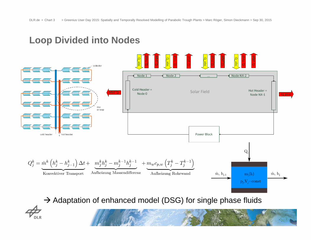
Loop Divided into Nodes


Adaptation of enhanced model (DSG) for single phase fluids

Definition of Heat Loss Coefficients


Output of Results


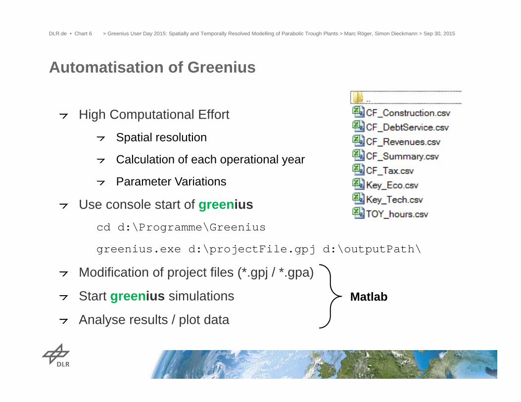
High Computational Effort

Spatial resolution

Calculation of each operational year

Parameter Variations

Use console start of greeniuscd d:\Programme\Greenius

greenius.exe d:\projectFile.gpj d:\outputPath\

Modification of project files (*.gpj / *.gpa)

Start greenius simulations

Analyse results / plot data

Automatisation of Greenius


Matlab

..\Greenius\data\project.gpj

..\Greenius\data\Technology\Troughs\Collector\collectorFile.gpa

%CMPDATADIR = Default Component Directory

Console Start


Technical Background of Receiver ReplacementStudy, Methodology and Results

Speaker: Marc Rö[email protected]

Overview

1. MOTIVATION of Study2. REFERENCE Parabolic Trough Plant3. SCENARIOS for Receiver Performance Loss4. METHODOLOGY & SOFTWARE greenius + Matlab5. RESULTS

DLR.de • Chart 9 > Greenius User Day 2015: Spatially and Temporally Resolved Modelling of Parabolic Trough Plants > Marc Röger, Simon Dieckmann > Sep 30, 2015

DLR.de • Chart 10

Field heat losses are between 7% (Jordan, Ma’an)and 10% (Guadix, Spain) of the collected solar energy(Eurotrough-type, 70mm absorber, HTF: Oil)

1. MOTIVATION of Study

> Greenius User Day 2015: Spatially and Temporally Resolved Modelling of Parabolic Trough Plants > Marc Röger, Simon Dieckmann > Sep 30, 2015

Labor

Receiver design lifetime is 20-40 yearsHowever, lifetime may be reduced by

Different maturity of productsLimited experience in operationIncreasing temperatures and new fluidsWind events with glass breakage

In case of failure, receiver heat loss may be increased by a factor 5 to 10

Objective of study: Energetic and economic impact of different receiver performance loss scenarios

DLR.de • Chart 11

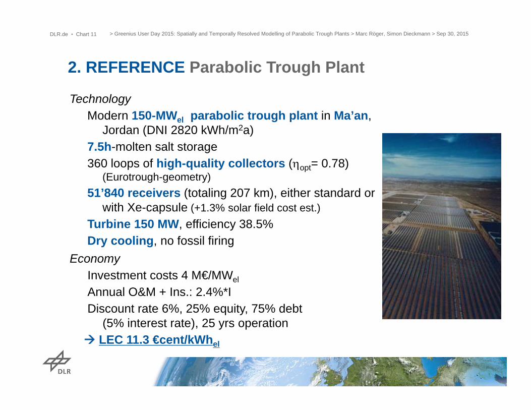
TechnologyModern 150-MWel parabolic trough plant in Ma’an,

Jordan (DNI 2820 kWh/m2a)7.5h-molten salt storage360 loops of high-quality collectors (opt= 0.78)

(Eurotrough-geometry)51’840 receivers (totaling 207 km), either standard or

with Xe-capsule (+1.3% solar field cost est.)Turbine 150 MW, efficiency 38.5%Dry cooling, no fossil firing

2. REFERENCE Parabolic Trough Plant


EconomyInvestment costs 4 M€/MWel

Annual O&M + Ins.: 2.4%*IDiscount rate 6%, 25% equity, 75% debt

(5% interest rate), 25 yrs operation LEC 11.3 €cent/kWhel

DLR.de • Chart 12

Event“Wind A/B” Wind event destroying glass envelopes“H2” Hydrogen accumulation“AR” Anti-reflection coating degradation

3. SCENARIOS for Receiver Performance Loss


Variation of point in time when damage occurssudden event year t=5, 10, or 15gradual damage (AR) 1..5, 1..10, 1..15

Different counter measures (full performance in year t+2)“Leave” damaged receivers (do nothing)“Replace” damaged receiversActivate “Xenon” capsule (H2 accumulation)“Fix” receivers (H2 accumulation)

Affected Field50% (H2) or 100% (AR) of fieldLimits of field (5.6%, Wind)

DLR.de • Chart 13

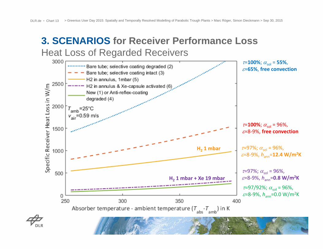
3. SCENARIOS for Receiver Performance LossHeat Loss of Regarded Receivers


=100%; sol = 55%,=65%, free convection

=100%; sol = 96%,=8‐9%, free convection

=97%; sol = 96%,=8‐9%, hann=12.4 W/m2K

=97%; sol = 96%,=8‐9%, hann=0.8 W/m2K

=97/92%; sol = 96%,=8‐9%, hann=0.0 W/m2K

H2 1 mbar

H2 1 mbar + Xe 19 mbar

DLR.de • Chart 15

4. METHODOLOGYgreenius + Matlab


DLR.de • Chart 16



DLR.de • Chart 17



DLR.de • Chart 18



DLR.de • Chart 19

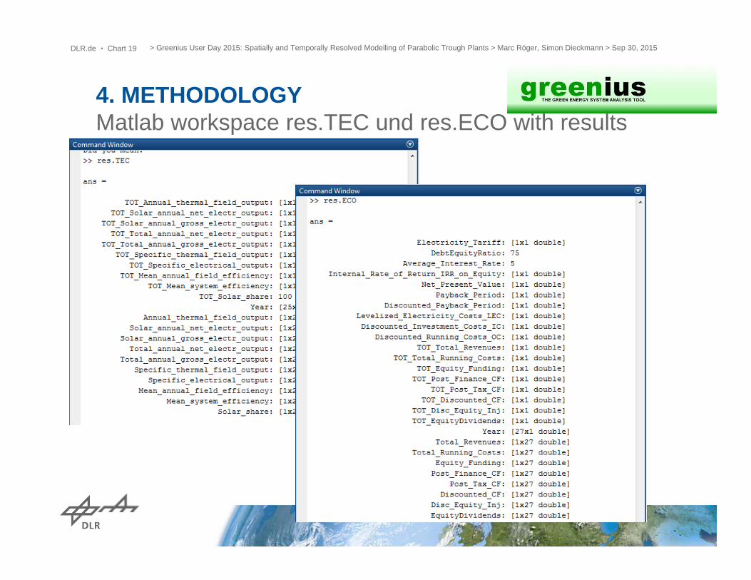
4. METHODOLOGYMatlab workspace res.TEC und res.ECO with results


DLR.de • Chart 20

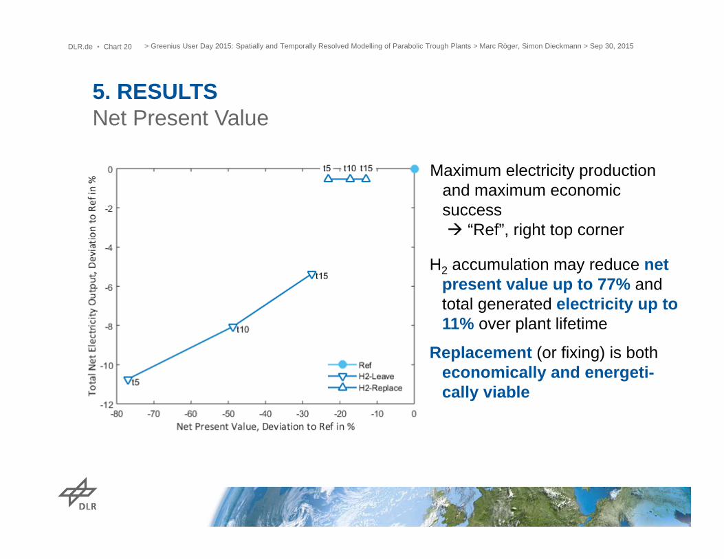
5. RESULTSNet Present Value


Maximum electricity production and maximum economic success “Ref”, right top corner

H2 accumulation may reduce net present value up to 77% and total generated electricity up to 11% over plant lifetime

Replacement (or fixing) is both economically and energeti-cally viable

DLR.de • Chart 21

5. RESULTS


More results will be presented at the SolarPACES conference 201513.-16.10.15, Cape Town

Successful adaptation of greenius for varying heat losses over loop and operating time

Similar implementation for public version is planned see presentation on current development

Console start for greenius calculations without GUI

Matlab can be used to…

Set up project files

Start simulations

Analyse results

Conclusion


DLR.de • Chart 23

THANK YOUfor your attention.

We gratefully acknowledge the financial support from the German Federal Ministry for Economic Affairs and Energy for the two projects:‐ PARESO: Contract no. 0325412‐ FreeGreenius: Contract no. 0325427

Spatially and Temporally Resolved Modeling of Parabolic Trough ...

Documents

Transcript of Spatially and Temporally Resolved Modeling of Parabolic Trough ...